magnetic resonance imaging- based radiation therapy treatment
TRANSCRIPT
Master’s Thesis
Physics
Magnetic resonance imaging- based radiation therapy treatment planning
Lauri Koivula2016
Supervisors: D.Sc. (Tech.) Juha Korhonen Doc. Mikko Tenhunen
Examiners: Prof. Sauli Savolainen Doc. Mikko Tenhunen
UNIVERSITY OF HELSINKIDEPARTMENT OF PHYSICS
P.O. Box 64 (Gustaf Hällströmin katu 2 A)00014 University of Helsinki

3
Tiedekunta/Osasto Fakultet/Sektion – Faculty Faculty of science
Laitos/Institution– Department Department of Physics
Tekijä/Författare – Author Lauri Koivula Työn nimi / Arbetets titel – Title Magnetic resonance imaging- based radiation therapy treatment planning Oppiaine /Läroämne – Subject Physics Työn laji/Arbetets art – Level Master’s Thesis
Aika/Datum – Month and year February 2016
Sivumäärä/ Sidoantal – Number of pages 38
Tiivistelmä/Referat – Abstract This work studied the conversion of the magnetic resonance images to synthetic heterogeneous computed tomography (CT) images, so-called pseudo-CT images. The study focused on updating and modifying a previously introduced conversion technique. Ultimate objective of this study was to verify the technique after a hardware and software update of the MR scanner. This included adjustments of the image conversion algorithms and integration of these into a medical image processing software. Additionally, this work aimed to use automatic bone segmentation atlas with the technique. The updated technique was verified for prostate cancer patients. This work aimed also to evaluate possibilities to adopt the technique for other patient groups and with different MR scanner. The evaluation included measurement for geometric accuracy in MR images. Average local difference in Hounsfield units (HU) between pseudo-CT and actual CT images for soft- and bony tissues were -1±13 HU and -10±139 HU, respectively. Measurement points in soft tissue had coverage of 89 % with smaller absolute error than 20 HUs. In bony tissue average of 88 % of the measurement points were within 200 HU error margin. The dose difference between pseudo-CT and actual CT images was -0.4 % ± 0.2%. Dose difference in PTV for automated bone contouring against user corrected bone volumes was 0.1 % ± 0.1 %. The calculated dose in heterogeneous pseudo-CT was shown statistically significantly (p = 0.0014) more accurate compared to that in simplified pseudo-CT. The geometric error was within 1.1 mm for distances shorter than 20 cm from isocenter with two scanners. Preliminary pseudo-CT images were created with modified conversion algorithms for thigh and abdomen. Magnetic resonance imaging- based radiation therapy treatment planning provides reliable method for radiotherapy treatment in pelvic areas reaching the requirements in patient care. This study showed that the MR image conversion technique can be adjusted in case of updates in MR platform. The examinations suggested also that it seems doable to adopt the MR image conversion technique to different body parts and with different MR scanners.
Avainsanat – Nyckelord – Keywords Pseudo-CT, radiation therapy, radiation therapy treatment planning, dual model HU conversion model, dose calculations, magnetic resonance imaging, computed tomography
Ohjaajat – Handledare – Supervisor s Mikko Tenhunen, Juha Korhonen
Säilytyspaikka – Förvaringställe – Where deposited
Muita tietoja – Övriga uppgifter – Additional information
4
Tiedekunta/Osasto Fakultet/Sektion – Faculty Matemaattis-luonnontieteellinen tiedekunta
Laitos/Institution– Department Fysiikan laitos
Tekijä/Författare – Author Lauri Koivula Työn nimi / Arbetets titel – Title Magneettikuvaus –pohjainen sädehoidon suunnittelu Oppiaine /Läroämne – Subject Fysiikka Työn laji/Arbetets art – Level Pro gradu -tutkielma
Aika/Datum – Month and year Helmikuu 2016
Sivumäärä/ Sidoantal – Number of pages 38
Tiivistelmä/Referat – Abstract Tämä työ käsittelee mahdollisuutta muokata magneettikuvista synteettisiä, heterogeenisia tietokone-tomografia (TT)- kuvia, niin kutsuttuja pseudo-TT-kuvia. Tutkimuksessa keskityttiin ajantasaistamaan ja muokkaamaan jo olemassa olevaa konversiomallia laitteiston päivityksen jälkeen. Tämän työn tavoitteena oli tutkia magneettikuvien absoluuttisia intensiteettejä laitepäivityksen jälkeen ja muodostaa uudet konversiomallit pseudo-TT-kuvien luomista varten. Nämä toimintamallit lisättiin lääketieteellisten kuvien käsittelyohjelmaan. Luun pinnan automaattista määritystä tutkittiin vertailemalla simuloituja annoslaskenta-eroja käyttäjän korjaamien ja tietokoneen luomien luutilavuuksien välillä. Päivitetty tekniikka varmennettiin kymmenellä eturauhassyöpäpotilaalla takautuvasti. Työssä tutkittiin myös mallin kliiniseen käyttöön liittyviä näkökohtia, kuten konversiomallin toimivuutta eri potilailla ja magneettikuvauslaitteilla sekä geometrisen vääristymän vaikutusta annoslaskentaan. TT- ja pseudo-TT-kuvien keskimääräinen paikallinen ero Hounsfield yksiköissä (HU) pehmyt- ja luukudoksissa oli -1±13 HU:ta ja -10±139 HU:ta, vastaavasti. Pehmytkudoksessa keskimäärin 89 prosenttia tarkastelupisteistä oli 20 HU-yksikön virhemarginaalissa. Luukudoksessa 200 HU:n virhemarginaalissa oli keskimäärin 88 prosenttia tarkastelupisteistä. Kohdealueen keskimääräisen annoksen keskiarvo TT- ja pseudo-TT-kuvien välillä (TT – pseudo-TT) intensiteetti-muokatun sädehoidon tapauksessa oli -0,4 % keskihajonnan ollessa 0,2 %. Heterogeenisen mallin mukaan laskettu annos kohdetilavuudessa vastasi merkitsevästi (p=0,0014) paremmin TT-kuviin laskettua annosta kuin homogeeniseen malliin laskettuna. Pseudo-TT-kuviin lasketut annoserot kohdetilavuudessa olivat 0,1±0,1 %, vertailtaessa automaattista ja käsin korjattua luun pinnan määritystä. Isosentrin ympäristössä alle 200 mm säteellä geometrinen vääristymä oli vähemmän kuin 1,1 mm kahdella eri magneettikuvauslaitteella. Alustavat testikonversiot muodostettiin reiden ja alavatsan alueesta. Tämä työ osoittaa magneettikuvaukseen perustuvan sädehoidon suunnittelun olevan mahdollista toteuttaa lantion alueella potilashoidon asettamien rajojen puitteissa. Konversiomalli pystytään mahdollisesti laajentamaan kattamaan myös muita kehon osia. Tämä työ osoitti, että konversiotekniikkaa voidaan muokata laitepäivityksen jälkeen. Mallin selkeys voi mahdollistaa myös muiden kuvaussekvenssien ja magneettikuvauslaitteiden hyödyntämisen tulevaisuudessa pseudo-TT-kuvien luomisessa.
Avainsanat – Nyckelord – Keywords Synteettinen CT, sädehoito, sädehoidon suunnittelu, kaksiosainen HU konversiomalli, annoslaskenta, magneettikuvaus, tietokonetomografia Säilytyspaikka – Förvaringställe – Where deposited Muita tietoja – Övriga uppgifter – Additional information

5
Acknowledgements
I would like to thank Docent Mikko Tenhunen1 for giving me an opportunity to join this interesting research group and Doctor of technology Juha Korhonen1 for guiding me through the research process. He has been an excellent supervisor on the thesis and introduced the field of radiotherapy and the whole of medical phycis for me. During the project I received immeasurable amount of support and aid from everyone in the clinic, including all radiogra-phers, medical doctors and physicists, especially Tiina Seppälä. I would like to give a special thanks to Doctor Leonard Wee2,3 for valuable comments and assistance on the thesis, but also for the warm welcome and support during my eight weeks in Vejle, Denmark. My family and dear friends have given a lot strength during, sometimes laborous, writing period. Heinolan Hurjat© secured the necessary amount of humor in my life in the middle of my studies and thank you Tuomo and Simo for the peer support in our physicist residency. The most warmest thank you for my dear Elina, you have been an irreplaceable part of my life and without your influence this work would not have been made.
Affliations:
1Comprehensive Cancer Center, Helsinki University Hospital2Department of Medical Physics, Oncology Services, Vejle Hospital, Kabbeltoft 25, Vejle 7100, Denmark3Danish Colorectal Cancer Center South, Kabbeltoft 25, Vejle 7100, Denmark

6
“And a lean, silent figure lowly fades into the gathering darkness, aware at last that in this world, with great power there must also come – great reponsibility!”
– Stan Lee, Amazing Fantasy #15, 1962
7
Contents
Abstract 3Abstract in Finnish 4Acknowledgements 4Table of contents 7Lists of symbols and abbreviations 9
1. Introduction 1.1 Radiation therapy in cancer treatment 10 1.2 Radiation therapy treatment planning 10 1.3 MRI-only workflow 10 1.4 Geometrical distortion 11 1.5 Conversion from MRI to pseudo-CT images 12 1.6 Aims of the study 13
2. Materials and methods 2.1 Updated dual model HU conversion technique 14 2.1.1 Soft tissue conversion model 14 2.1.2 Bony tissue conversion model 15 2.2 Pseudo-CT image generation process 15 2.2.1 Automatic atlas-based bone segmentation 17 2.2.2 Application of the dual model HU conversion technique 17 2.3 Evaluating the quality of the constructed pseudo-CT images 18 2.3.1 HU accuracy in the pseudo-CT images 18 2.3.2 Dose calculations in pseudo-CT images 19 2.4 Procedure for evaluating geometrical distortion 20 2.4.1 Manual method with a “Lego phantom” 20 2.4.2 Automated method with grid phantom 21 2.5 Preliminary tests to adopt HU conversion technique with 23 different sequences and in various body parts
3. Results 3.1 Updated dual model HU conversion technique 24 3.1.1 Conversion curve for soft tissue 24 3.1.2 Conversion curve for bone segments 26 3.2 Example of the pseudo-CT image generation 28 3.3 Properties of constructed pseudo-CT images 28 3.3.1 HU difference between pseudo-CT and CT images 28 3.3.2 Dose distribution in pseudo-CT images 33 3.4 Geometric accuracy using two different methods 38
8
3.4.1 Geometric accuracy with a “Lego phantom” 38 3.4.2 Grid phantom evaluation for geometrical distortion 39 3.5 Test images of various body parts with different MRI sequences 42
4. Discussion 4.1 Conversion creation 43 4.2 HU-comparison 43 4.3 Dose comparison and radiation therapy planning 44 4.4 Geometric distortion measurements 44 4.5 Normalization and other clinical aspects concerning conversion 45 4.6 Reflection against other synthetic-CT conversion methods 45
5. Conclusions 47
References 48Appendix 51
9
Lists of symbols and abbreviations
ADNI Alzheimer’s disease neuroimaging initiativeART Adaptive radiation therapyCBCT Cone-beam computed tomographyCT Computed tomographyDVH Dose volume histogramDICOM Digital Imaging and Communications in MedicineDRR Digitally reconstructed radiographsEBRT External beam radiation therapyED Electron densityFOV Field of viewHU Hounsfield unitHUH Helsinki university hospitalIGRT Image-guided radiation therapyIMRT Intensity modulated radiation therapyMIM Medical imaging softwareMRI Magnetic resonance imagingMV MegavoltsPTV Planning target volumeR Language and environment for statistical computing and graphicsr Distance from isocenterROI Region of interestRT Radiation therapyRTP Radiation therapy treatment planningTE Echo timeTR Repetition time
10
Introduction
1.1 Radiation therapy in cancer treatment
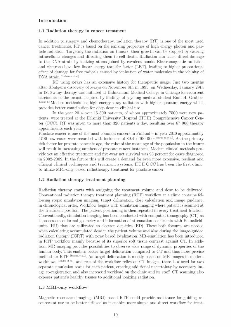
In addition to surgery and chemotherapy, radiation therapy (RT) is one of the most used cancer treatments. RT is based on the ionizing properties of high energy photon and par-ticle radiation. Targeting the radiation on tumors, their growth can be stopped by causing intracellular changes and directing them to cell death. Radiation can cause direct damage to the DNA strain by ionizing atoms joined by covalent bonds. Electromagnetic radiation and electrons have low linear energy transfer factor (LET), leading to higher proportional effect of damage for free radicals caused by ionization of water molecules in the vicinity of DNA strain.[Tenhunen et al.]
RT using x-rays has an extensive history for therapeutic usage. Just two months after Röntgen’s discovery of x-rays on November 8th in 1895, on Wednesday, January 29th in 1896 x-ray therapy was initiated at Hahnemann Medical College in Chicago for recurrent carcinoma of the breast, inspired by findings of a young medical student Emil H. Grubbe. [Evans T.] Modern methods use high energy x-ray radiation with higher quantum energy which provides better contribution for deep dose in clinical use. In the year 2014 over 15 500 patients, of whom approximately 7500 were new pa-tients, were treated at the Helsinki University Hospital (HUH) Comprehensive Cancer Cen-ter (CCC). RT was given to more than 320 patients a day, resulting over 67 000 therapy appointments each year. Prostate cancer is one of the most common cancers in Finland – in year 2010 approximately 4700 new cases were recorded with incidence of 89.4 / 100 000[Joensuu H. et al]. As the primary risk factor for prostate cancer is age, the raise of the mean age of the population in the future will result in increasing numbers of prostate cancer instances. Modern clinical methods pro-vide yet an effective treatment and five-year net survival was 93 percent for cases diagnosed in 2002-2009. In the future this will create a demand for even more extensive, resilient and effcient c linical techniques and treatment systems. HUH CCC has been the fi rst c linic to utilize MRI-only based radiotherapy treatment for prostate cancer.
1.2 Radiation therapy treatment planning
Radiation therapy starts with assigning the treatment volume and dose to be delivered. Conventional radiation therapy treatment planning (RTP) workflow at a clinic contains fol-lowing steps: simulation imaging, target delineation, dose calculation and image guidance, in chronological order. Workflow begins with simulation imaging where patient is scanned at the treatment position. The patient positioning is then repeated in every treatment fraction. Conventionally, simulation imaging has been conducted with computed tomography (CT) as it possesses conformal geometry and information of attenuation coeffcients with Hounsfield units (HU) that are calibrated to electron densities (ED). These both features are needed when calculating accumulated dose in the patient volume and also during the image-guided radiation therapy (IGRT) with x-ray based localization. MR-simulation has been introduced in RTP workflow mainly because of its superior soft tissue contrast against CT. In addi-tion, MR imaging provides possibilities to observe wide range of dynamic properties of the human body. This enables better target delineation compared to CT and thus more precise method for RTP [Sciarra et al.]. As target delineation is mostly based on MR images in modern workflows [Sander et al.], and rest of the workflow relies on CT images, there is a need for two separate simulation scans for each patient, creating additional uncertainty by necessary im-age co-registration and also increased workload on the clinic and its staff. CT scanning also exposes patient’s healthy tissues to additional ionizing radiation.
1.3 MRI-only workflow
Magnetic resonance imaging- (MRI) based RTP could provide assistance for guiding re-sources at use to be better utilized as it enables more simple and direct workflow for treat-
11
ment planning as no additional CT scans are needed with MR-CT co-registration. Using MR imaging as an only imaging modality in RTP workflow additional requirements has to be met – geometrical accuracy has to be adequate compared to CT and a method to produce reliable electron density distribution in the patient image is needed. Scanner with a flat table top and coil bridges are required to prevent the body exterior alterations if laying receiver coils directly on the patient skin. External orthogonal laser-localization system is needed for tattooing treatment isocenter localization markers on the patient skin. MR-compatible immobilization devices which enables similar patient positioning also in CT scanning and treatment are necessity. In conventional RT with linear accelerator equipped with cone-beam CT (CBCT) or planar localization images, pseudo-CT images can be used for IGRT as 2D reference DRRs or volumetric co-registration between RTP images and CBCT localization images. Newly developed techniques with MR scanner integrated with treatment hardware, such as linear accelerator (MRI-Linac) [Raaymakers et al.] or Cobalt-60 radiation source [Kron et al.] (MRI-60Co sys-tem, ViewRay®, Oakwood Village, OH, USA), could provide online adaptive RT (ART) and automatic MR-to-MR image co-registration between the RTP- and localization images – MRI guided RT (MRIgRT). Also moveable MR scanner [Stanescu et al.] or interchangeable MRI table trolley [Karlsson et al.] integrated with linac have been proposed in previous studies.
1.4 Geometrical distortion
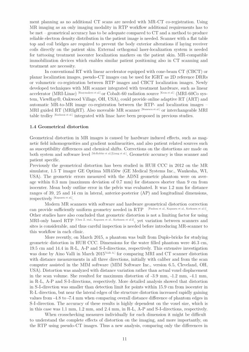
Geometrical distortion in MR images is caused by hardware induced effects, such as mag-netic field inhomogeneities and gradient nonlinearities, and also patient related sources such as susceptibility differences and chemical shifts. Corrections on the distortions are made on both system and software level [McRobbie et al.][Liang et al.]. Geometric accuracy is thus scanner and patient specific. Previously the geometrical distortion has been studied in HUH CCC in 2012 on the MR simulator, 1.5 T imager GE Optima MR450w (GE Medical Systems Inc., Waukesha, WI, USA). The geometric errors measured with the ADNI geometric phantom were on aver-age within 0.3 mm (maximum deviation of 0.7 mm) for distances shorter than 9 cm from isocenter. Mean body outline error in the pelvis was evaluated. It was 1.2 mm for distance ranges of 39, 25 and 14 cm in lateral, anterior-posterior (AP) and longitudinal dimensions, respectively [Kapanen et al.]. Modern MR scanners with software and hardware geometrical distortion correction can provide suffciently uniform geometry needed in RTP [Paulson et al., Kapanen et al., Korhonen et al.1].Other studies have also concluded that geometric distortion is not a limiting factor for using MRI-only based RTP [Chen Z. etal., Kapanen et al., Korhonen et al.2], yet variation between scanners and sites is considerable, and thus careful inspection is needed before introducing MR-scanner to this workflow in each clinic. More recently, on March 2015, a phantom was built from Duplo-bricks for studying geometric distortion in HUH CCC. Dimensions for the water filled phantom were 46.3 cm, 19.5 cm and 14.4 in R-L, A-P and S-I-directions, respectively. This extensive investigation was done by Aino Valli in March 2015[Valli A.] for comparing MRI and CT scanner distortion with distance measurements in all three directions, initially with caliber and from the scan computer assisted in the MIM software (MIM Software Inc., version 6.5, Cleveland, OH, USA). Distortion was analyzed with distance variation rather than actual voxel displacement in the scan volume. She resulted for maximum distortion of -3.9 mm, -1.2 mm, -4.1 mm, in R-L, A-P and S-I-directions, respectively. More detailed analysis showed that distortion in S-I-direction was smaller than detection limit for points within 15.9 cm from isocenter in R-L direction, but near the lateral edges of the structure distortion increased rapidly gaining values from -4.8 to -7.4 mm when comparing overall distance difference of phantom edges in S-I-direction. The accuracy of these results is highly dependent on the voxel size, which is in this case was 1.1 mm, 1.2 mm, and 2.4 mm, in R-L, A-P and S-I-directions, respectively. When crosschecking measures individually for each dimension it might be diffcult to understand the complete effects of distortion on the imaging, and more importantly, on the RTP using pseudo-CT images. Thus a new analysis, comparing only the differences in
12
distance between isocenter and simulated body contour, was made on the same images that have been previously used.
1.5 Conversion from MRI to pseudo-CT images
The pelvic volume of human body contains variation of tissues such as adipose tissue, urine, muscle, cortical bone [White et al] - with different HU values ranging ~ -100, 10, 50, 1500, respec-tively, corresponding to ED values of ~0.90 to 1.90 in relation to water [Schneider U. et al.]. Strong heterogeneity is present and it has a great effect on the dose distribution with a diverse patient spectrum. If using only MRI-based methods, these ED values are needed to map to corresponding tissues, and create so-called pseudo-CT for achieving correct dose calcula-tions results and possibility to use digitally reconstructed radiographs (DRR) in planar 2D IGRT and voxel-based HU data for 3D/6D IGRT. The first suggested methods for creating pseudo-CT images, utilizing MR-images in RTP were water-only and bulk methods. Pseudo-CT images contain approximation of the HU values and EDs of the tissue. Water-only images represent whole patient volume as water-equivalent and bulk images give single pseudo-HU value for bone segment and soft tissues separately [Lee et al., Pasquier et al.]. Eilertsen et al. suggested contouring only the densest bone and assigning it with single ED-value and everything else with water equivalent. Prior studies in HUH CCC have demonstrated it is possible to create heterogeneous pseudo-CT of pelvis using MR-images in clinical use [Kapanen & Tenhunen][Korhonen et al.3][Korhonen]. With this approach, clinically acceptable results were obtained in dose calculations - average deviation of 0.3 % for mean planning target volume (PTV) dose for 20 patients – and in image guidance – stan-dard deviation in patient position corrections were smaller than 0.9 mm and 0.7° (translation and rotation, respectively) – when compared to original simulation images conducted with CT[Korhonen]. Conversion implemented in clinical workflow in HUH involves automated bone con-touring, definition of scan-specific normalization factor and automatic conversion workflow inside the software with manual verification of pseudo-CT images. Bone contouring is done by atlas-based method which is provided by the MIM software. Normalization factor, which defines the overall average MR image intensity level of each scan, is detected from predeter-mined location of the patient and corresponding workflow is then selected from conversion library. Numerical value of the normalization factor is the average muscle tissue intensity value in particular scan. After the automatic HU value assigning, manual setting of HU values for internal fiducial gold markers is needed. Seeds are visible in MR images and the volumes can be contoured manually by physicist.
1.6 Aims of the study
The dual model HU conversion method demonstrated by Korhonen et al. is dependent on the absolute intensity values of the MR image as the pseudo-CT is produced by directly assigning predetermined HU values for MR image intensity ranges. Thus any change on the original MR intensity values will hinder the functionality of the conversion. Small variation occurs in every scan due to imperfections in the image acquisition and intensity correction – effect of these variations is examined in this study. MR scanner hardware or software up-dates can also give rise to a systematic change intensity value alterations – this was the case with given scanner in HUH CCC. A substantial update was performed and absolute MR images intensity values and dynamic range shifted in patient images – this created a need for revising and updating the conversion workflow. Clinical interest on synthetic-CT creation and employing MRI-only methods in RTP are increased greatly during the last years – with keywords “synthetic-CT” and “pseu-do-CT”, there are 27 articles found in PubMed (United States National Library of Medicine, National Institutes of Health, “pubmed.gov”) published between January 2014 and Decem-ber 2015. These studies include work on novel conversion algorithms [Korhonen et al.3][Kim J. et al.1]
[Siversson C. et al][Andreasen D. et al.], detection of bone contours and separating air volumes [Korhonen et al.2][Liu
L. et al.][Zheng W. et al.][Hsu S. et al.], dosimetric accuracy in different sites of the body [Korhonen et al.1][Korhonen

13
et al.4][Kim J. et al.2][Paradis E. et al.][Jonsson J. et al.] and adaptive methods [Whelan B. et al.]. Published synthetic-CT conversion techniques have variable methods for transform-ing MR image intensity values to HUs. Both clinical and pre-clinical sequences are utilized, such as T1- or T2-weighted [Kim J. et al.1] and ultra-short echo time (UTE) sequences [Edmund J. M. et
al.], respectively. Multiple different techniques have been implemented for the image intensity value conversion itself, including manual voxel-based methods [Korhonen et al.3][Kim J. et al.1] and atlas-based approaches [Andreasen D. et al.][Dowling et al.]. Although the methods vary, results concerning dose comparison and difference in HU values between CT and pseudo-CT are consistent and on the same scale. Majority of the published techniques achieve PTV dose differences between CT and pseudo-CT below one percent [Korhonen et al.3][Kim J. et al.1] [Andreasen D. et al.]. Good results are also possible to obtain with simple and unsophisticated manual techniques using clinical MR scanning sequences [Korhonen et al.3][Kim J. et al.1]. As many of these researches are in development phase, there has been minimal attention on the calculation time and the clinical usability of the method. This study aims to utilize fast and pragmatic user interface for the conver-sion in clinical practice. These aspects are then compared among the presented method and previously published methods. Previous research is mainly focused on head and pelvic volumes and methods pro-vided limited usage for different body parts. Thus, the study aims to evaluate preliminary methods and feasibility of adopting the dual model HU conversion technique for pseudo-CT generation with different sequences and in other body parts. The main objective of this thesis is to provide updated conversion models for pseudo-CT creation for clinical use. Additionally, the normalization factor acquiring process is to be evaluated and studying the effect of MR intensity value variation in the patient cohort on the conversion and finding novel conversion curves for different intensity levels. Automatic bone contouring process is to be revised and its fidelity compared to manual contouring is examined. Renewed pseudo-CTs are then objected to HU evaluation and dose calculation comparison. Two different methods for inspecting geometric distortion on the MR scanner are introduced.
14
Materials and methods
Patient groups
Two separate groups containing 10 prostate cancer patients with clinically used CT and MR RTP simulation images with each patient were used in this study. Images were collected during normal clinical RT and no clearly visible artifacts were present. The investigation did not have any effect on the RTP of the patients and was done mainly retrospectively. Evaluating necessary standard of registration between images was performed and clearly misaligned cases were dismissed. First group (data group) was used for conversion model generation and second group (test group) for pseudo-CT images reconstruction. For each group a wide variety of absolute MR image intensity levels was selected as the order of the overall absolute MR intensity of images can have an impact in pseudo-CT conversion.
Imaging
CT and MR imaging followed the general requirements of RT patient positioning in clinical use. This was achieved with immobilization employed also in MR scanning with flat table top and coil frame to prevent coil-skin contact, creating similar patient geometry than in RT delivery. MR scanner was 1.5 T imager GE Optima MR450w (GE Medical Systems Inc., Waukesha, WI, USA) and a T1/T2*-weighted in-phase MR image set was produced with a 3D fast RF-spoiled dual gradient echo sequence (LAVA Flex ®) [Ma J.] and water-only image series from computationally generated from in-phase and out-of-phase images from the same scan [Dixon W.T.]. In-phase series’ absolute image intensity values were utilized in pseudo-CT conversion and water-only images were used to create bone atlas for automatic bone contouring. The imaging parameters were 2.1 and 4.3 ms for the echo times (TE) (out-of-phase and in-phase signals, respectively), 6.8 ms for the repetition time (TR), 15° for the flip angle, and 90.9 kHz for the bandwidth. Field-of-view (FOV) for scan was set to 500×500 mm to obtain whole patient geometry even with larger patients. Matrix size was 428×448, which was reconstructed in post-processing to 512×512 resolution. The pixel size was 0.98×0.98 mm2 and the slice thickness was 2.4 mm. Average scan time in MRI was 3 min and 17 s. CT scanning was conducted with GE LightSpeed RT with settings of 120 kVp, 500 mm data collection diameter (reconstruction matrix of 512×512) resulting pixel size of 0.98×0.98 mm2 and slice thickness of 2.5 mm.
2.1 Updated dual model HU conversion technique
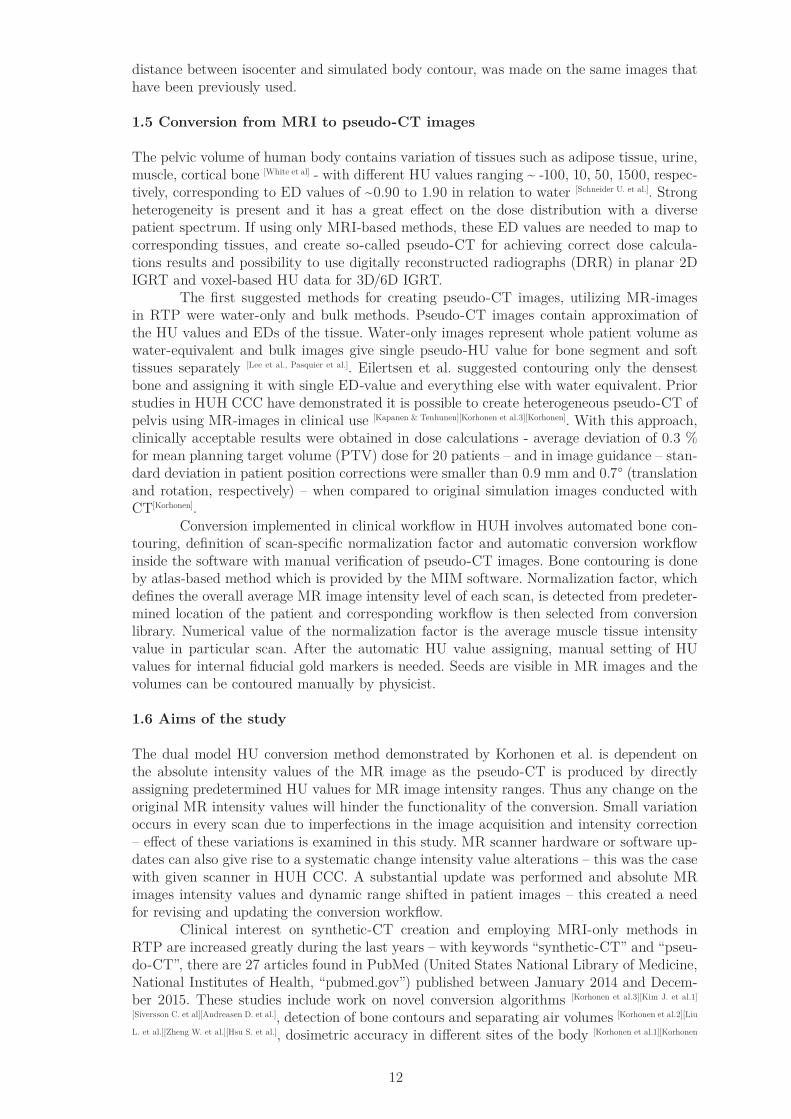
The same conversion generation technique was used as previously discovered feasible for the Helsinki scanner [Korhonen et al.3]. Method relies on comparing absolute MR image intensity values to measured CT image HU values of rigidly co-registered image stacks. Conversion parameters are different for segments inside and outside of bone contour because of MR intensity values overlap for certain tissue types, such as high density bone and urine. This leads to a dual model HU conversion for soft tissues and bone separately. Co-registration was done automatically by the MIM software. User defined manually the volume of box-based co-registration for each patient - main pelvic bones around prostate: femoral head, ilium and pubis – as these areas contain high heterogeneity and successful co-registration is needed for conversion curve generation. Minor misregistration in adipose tissue or muscle volumes does not affect greatly on voxel intensity correspondence between CT and MR but even a fine misalignment in cortical bone volumes has influence on the conversion curve. Figure 1 presents data collection region-of-interests (ROIs) on a transversal slice of co-registered MR and CT images.
2.1.1 Soft tissue conversion model
Data collection ROIs were placed over the entire patient volume – around the FOV on three different slices with 3 cm gaps - to correspond the intensity fluctuations occurring in the MR
15
image stack and to gather well presented data of the volume that is important clinically for prostate cancer RT. Pubic symphysis was assigned as reference point in the longitudinal di-rection – three data collection slices were with relation to it by 1 cm cranially and 2 cm and 5 cm caudally. Tissue types collected were: muscle (30), prostate (10), rectal wall (10), urine (10) with subcutaneous (30) and visceral fat (10). For each patient 100 of these data points were collected and altogether 1000 reference points were used for conversion model genera-tion. Bulk values of HU were set for segments of urine, muscle and fat with range obtained from MR image intensity mean with standard deviation for each tissue type – possible gaps between intensity range of each tissues were interpolated linearly to HUs [Korhonen et al.3].
2.1.2 Bony tissue conversion model
Four different tissue types were arranged for data collection: cortical bone (20 for each patient), bone marrow (20) with dense spongy bone (10) and low density spongy bone (10). Spongy bone ROIs were investigated only in the femoral head but cortical bone and bone marrow were collected from femur and ilium at various sites. A three variable exponential fitting was made for all 600 data collection ROIs obtained and fine-tuned manually for bet-ter correspondence at the spongy bone intensity scale based on the variation on the data and previously used conversion curves.
2.2 Pseudo-CT image generation process
In-phase image and its absolute intensity values were used for the pseudo-CT conversion with water image aiding the bone contouring process. When creating pseudo-CTs from MR image, patients might have a slightly different position when comparing to CT images and this will affect the body outline position. The body position differences were considered by creating the pseudo-CTs as described in the Figure 2. Areas inside CT body contour but outside MR exterior were labeled as water (HU = 0) and segments that were inside MR but outside CT were set as air (HU = -1000). Total of three heterogeneous pseudo-CTs were created to evaluate different clinical aspects of using pseudo-CTs in patient RTP workflow. Either body contour of MR or CT images was used with bone segment contoured automatically or manually by the author. Figure 3 presents an illustration for reviewing similarities and differences between dose comparisons. The accuracy of the atlas-based bone contouring was studied by comparing dose differences between images #1 and #2 (ΔD12). Dose comparison was also executed for studying variation caused by changes in patient body outline between scans (ΔD23) and most importantly the pseudo-CT conversion model (ΔD34). So when comparing images 1 and 2, only difference in the models is different bone contouring – same body exterior and HU value conversion model is used in both images. Again, when comparing images 2 and 3, the only difference is the body contour used for
Figure 1: Axial slice on the 1 cm cranial position in reference to pubic symphysis. Co-registered image stacks with MR image on the left and CT on the right.

16
pseudo-CT construction (image 2 from MR series and image 3 from CT series). Most impor-tant comparison is then made between images 3 and 4 - pseudo-CT with CT image exterior contour and the original CT image – in this case only difference is the absolute HU values in the images, so conversion model can be evaluated. Those pseudo-CTs are named as follows:
#1. Pseudo Native atlas – uses atlas-based bone contouring with exterior contour obtained from MR image #2. Pseudo Native clinical – manually corrected atlas bone contouring with body contour from MR image#3. Pseudo CT-body clinical - manually corrected atlas bone contouring and body transferred from CT image#4. Original CT – CT image used for dose calculation comparison and from which CT body contour is copied from
Pseudo Native atlas Pseudo Native clinical Pseudo CT-body clinical Original CT image
#1 #2 #3 #4ΔD12 ΔD23 ΔD34
Figure 3: Three created pseudo-CTs with solid lines representing CT image body contour and manually con-toured bones. Dashed line presents body contour obtained from MR scan and automatically contoured bone segment.
In addition to these three heterogeneous pseudo-CT images, two homogeneous models (only water and water with bulk HU value bone contours) were created for evaluating the func-tionality of the heterogeneous pseudo-CT conversion against more simple models. Both images used exterior contour obtained from CT image and bone contours were clinically finalized similarly as in pseudo #3. An average HU value was calculated from original CT image for the bulk bone segment to minimize the dose differences created by absolute HU value differences and giving more impact for the actual homogeneous vs heterogeneous ef-fect. Comparing heterogeneous model and homogeneous ones, it is more important to ob-serve the dose difference variation than the average mean dose difference, since the bulk HU values on the models does not represent genuine patient data, but are merely simplifications. If selecting the same HU value for bulk tissues as average HU value in pseudo-CT images, it would result in smaller or negligible absolute dose difference between models, so analyses on variation give more insight on the feasibility of models compared to CT scan. Statistical comparison was made for IMRT plans by comparing dose difference of CT versus pseudo-CT to CT versus homogeneous models. F-test was conducted as the dose difference between models is created mostly because the differences in HU levels which were set manually and only variation between ten patients had clinical interest and was to be tested.
Figure 2: Example with over simplification of the situation.
1: Area of the MR image body contour that is outside CT body contour – manually labeled as HU = -1000 (air).2: CT body contour outside MR body – set as wa-ter equivalent with HU = 0 – thus included in the pseudo-CT image.3: Area where conversion is conducted.Everything outside areas 1-3 is labeled as air.
12
3
17
2.2.1 Automatic atlas-based bone segmentation
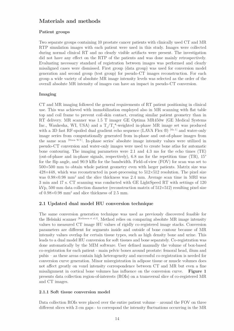
Dual model HU conversion requires the bone tissue contour for soft- and bony tissue sepa-ration. This was done by creating an atlas based on 10 patients water-only image series as bone tissue is presented with very low intensity range in the whole bone segment – addition to cortical bone also bone marrow and spongy bone appear dark on the water image due to fat suppression [Li X. et al.]. Figure 4 demonstrates this effect. According to preliminary tests conducted by author this can make automated atlas segmentation work more reliable and coherent fashion for a variety of patients compared to using in-phase images. Different software might withhold the vantage of water images. Bone-atlas was created by manual fine-contouring of cortical bone boundaries by the author for ten patients’ in-phase images. Contours were then transferred to water-only images and atlas saved in the software. Patient group used for atlas generation was different than ten test patients who pseudo-CTs were created. Automated atlas segmentation was done with a commercial medical image process-ing software MIM, by 5/10-method – meaning that software selected five best matching patients from the atlas, containing total of ten cases, and created bone contours based on these. Accuracy of the atlas segmentation was examined with dose calculation comparison to evaluate the effect of bone contours to target dose – dose for pseudo-CTs #1 and #2 were calculated with same RTP plan and dose differences in PTV were compared. Clinical manual correction in this case meant approximately 30 minutes of manual contouring based on the previously acquired atlas segmentation by a physicist with a Wacom drawing table (DTX2100, Wacom Technology Corporation, Vancouver, WA, USA). With software assisted manual contouring this time period enables precise bone edge determination for dose calcula-tion comparisons.
Figure 4: Water image from the LA-VAFlex series. Overall darker pre-sence for bones can be seen when comparing to the surrounding musc-les.
2.2.2 Application of the dual model HU conversion technique
Normalization of MR image intensity level
MRI intensity level is effected by such as patient size, receiver coil distance from the body and image correction algorithms. This will create variation between scans and patients lead-ing a need for normalization of the conversion curve. Ten different normalization levels were selected to cover all possible variation be-tween intensity levels. Soft tissue conversion curves were divided into eleven intensity ranges and conversion occurring inside bone contour was set to have 20 different HU value ranges. The maximum number of individual HU settings was mainly restricted by the hardware constraints – more intricate conversion would utilize memory and computational power more than is conceivable in the current system. Soft tissue conversion was expected to perform well even with smaller number of steps as the HU differences are smaller between muscle and adipose tissue than between cortical bone and bone marrow. For soft tissue conversion, steps between ranges were cal-
18
culated via linear interpolation between bulk value edges, and different normalization levels were distributed evenly for the range of 270-450 HUs, where there was data from the test patients. Intensity range step values, both in MR intensity scale and assigned HU-value, were set up based on the fitting on the overall data and previously used clinical conversion curves. Ten different normalization levels were equalized in relation to each other to even out the differences between adjacent levels.
Clinical workflow of pseudo-CT image generation
Conversion implemented in clinical workflow in HUCH involves automated bone contouring, definition of scan-specific normalization factor and automatic conversion workflow inside the software with manual verification of pseudo-CT images. Bone contouring is done by atlas-based method which is provided by the MIM software. Normalization factor, which defines the overall average MR image intensity level of each scan, is detected from predetermined location of the patient and corresponding workflow is then selected from conversion library. After the automatic HU value assignment, manual setting of HU values for internal fiducial gold markers is needed. Seeds are visible in MR images and the volumes can be contoured manually by physicist. Both soft- and bone tissue MRI to HU value conversions were implemented in a single software workflow. Clinical application of the conversion begins with copying the in-phase images and setting their DICOM header to CT, changing MR intensities to HU values in the software. This is followed by atlas based bone contouring. Water-only images from LAVAFlex series are subjected to atlas contouring and bone structures are then transferred to in-phase images. Before conversion a determination of overall MR image intensity in the in-phase images is needed. This is done by collecting four ROIs with diameter of 5 mm from obturator internus muscle near the prostate. Average of the intensity values from these four ROIs is considered as normalization factor for that particular scan. One conversion workflow from ten workflow library is selected according to the average intensity in the muscle tissue. After the conversion a qualitative inspection is performed by the user and gold seeds con-toured manually and HU value of 3000 set for enabling comparable DRR creation for IGRT.
Creation of water and homogeneous models
Average full bone volume HU value (HU = 358) was calculated form the CT images of ten patients which pseudo-CT images were also created. This mean value was used for the bulk value for bones in the homogeneous comparison models to minimize the effect of different HU levels between CT, pseudo-CT and homogeneous model dose comparisons. HU value of 0 was used for the soft tissue segment on the homogeneous model as it is commonly used also in other studies [Lee et al., Pasquier et al.] and it represents the average pelvic tissue set’s approxi-mate HU value between muscle and adipose tissue.
2.3 Evaluating the quality of the constructed pseudo-CT images
2.3.1 HU accuracy in the pseudo-CT images
The examination for reviewing HU differences were based on the same ROI-based method (160 ROIs per patient) as the conversion, meaning each conversion point were referenced against the same point in the original CT rather than studying the overall values in the image, in which case information about the functionality of the conversion would be lost. HU values were compared with both qualitative and quantitative means – former based on average differences and standard deviation with minimum and maximum and absolute HU value difference within predefined HU-value thresholds in particular tissue group for each patient, and latter based on histograms of gathered values with graphical presentation of all 1600 data points in a single figure. Mean relative differences and standard deviation were calculated from combined
19
data from all ten patients to observe the overall functionality of the pseudo-CT HU value conversion, when again absolute differences in the predefined HU value thresholds were evaluated casewise for examining the variation between patients. For all tissue types, both soft- and bony tissue, four windows were used, but more elaborate HU threshold windowing illustrating the change in full scale, with eight ranges, was done for ROI groups containing all soft tissue types (100 data points per patient) and all bony tissues (60 data points per patient). Soft tissue absolute HU value differences were binned with 5, 10, 15, 20, 25, 30, 40 and 50 HU value windows and bone tissues correspondingly with eight threshold bins of 25, 50, 75, 100, 150, 200, 300 and 400 HUs.
2.3.2 Dose calculations in pseudo-CT images
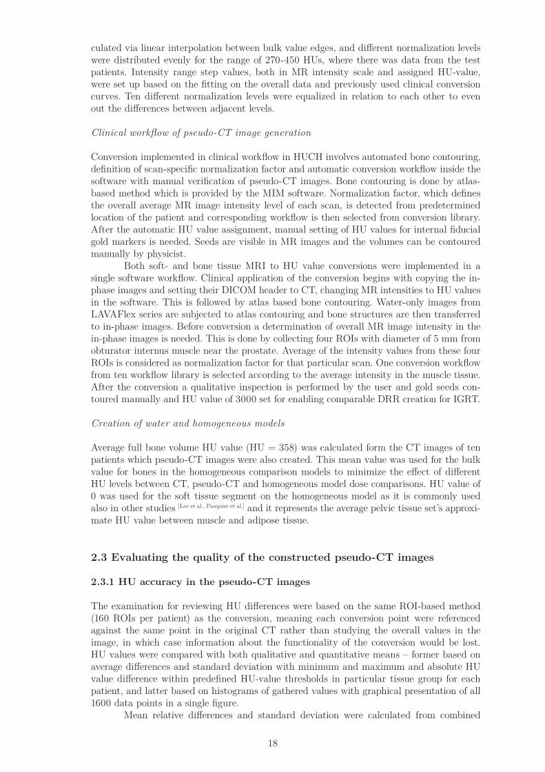
Primary RTP was conducted on the original CT series and then copied to corresponding pseudo-CT images of the same patient. If multiple PTVs were contoured for the patient, one with only containing prostate and not seminal vesicles was used as target for dose com-parison. Average PTV volume was 92 cm3 and smallest and largest PTVs were 52 and 143 cm3. Two types of RT were performed in each case: traditional four-field RT (BOX) was planned with beams arriving at gantry angles of 0, 90, 180 and 270 with static multi-leaf collimators. Intensity-modulated radiotherapy (IMRT) plans had seven individual beam directions distributed approximately evenly around the patient and non-uniform radiation fluence generated by inverse-planning process. Beam energy in all plans was set to 6 MV for maximizing dose differences resulting from attenuation differences. Plan calculations were executed with anisotropic analytical algorithm (AAA, Eclipse® 11.0, Varian Medical Sys-tems Inc., Helsinki, Finland). Examples from the plans with calculated dose are presented in Figure 5. Plan quality was not evaluated in detail for dose coverage in PTV, but simple and basic plans were applied as the dose difference was the only factor under investigation. Calculated dose distributions were compared in the planning target volume (PTV) at dose volume histogram (DVH) levels of 99, 95, 50, 5 and 1 volume percent and overall mean dose of the whole PTV.
Figure 5: Four-field plan (BOX) illustrated in transverse slice in figure A and seven-field plan (IMRT) in figure B.
BA
The absolute change between images #2 and #4 is composed from the pseudo-CT conver-sion (DΔ34) and changes in body outline (DΔ23) – Figure 3 shown in section 2.2 presents the visualization of the situation. Body outline changes between CT and MRI scans simulate the presence of small interfractional changes in body contour. It is possible to compare the proportional impact of the conversion and body outline effects and variation within each one. IMRT plan dose differences from both comparisons were summed as a total change and proportions in absolute difference were compared. Also qualitative review of the dose differ-ence was performed visually inside the planning software.
20
Effect of normalization for HU values in the pseudo-CT images
Variable absolute intensity levels among patients create a need for normalization – the same constant conversion curve is not possible to use with each patient but a method is needed to even out the differences. Previously a feasible normalization method for bony tissue was introduced by Korhonen et al[Korhonen et al.3]. and here this normalization technique is extended to involve soft tissue conversion also. Method relies on to evaluate the absolute MR intensity levels individually for each patient and previously they were collected from large muscles around the femur such as iliopsoas. Novel studies have indicated that intensity variation in a single patient image can be too big for reliable average absolute intensity value collection from muscles far away from the isocenter and near the body surface [Koivula L.], and muscles nearer the isocenter, such as obturator internus, can provide more regular and sound source for intensity normalization. Normalization for the conversion was achieved by shifting the conversion curve in the MR intensity scale in soft tissue conversion. Bony tissue conversion normalization was done in more sophisticated way by iterating curves in respect to previously used conversions in the clinic and with information gathered from average HU values inside the whole bone volume and comparing those to values of the original CT image. Fidelity and functionality of different normalization levels were evaluated by compar-ing average HU values in the femoral head and whole bone volume between original CT and pseudo-CT. Femoral head was contoured manually with spherical ROI with 1 mm marginal outside the cortical bone. Whole bone volume was contoured from original CT images with threshold of 150 HUs and then contour was rigidly copied to pseudo-CT image. Additionally the dose differences against pseudo-CTs were compared amongst normalizations to verify if any systematic changes are present. Pearson’s correlation coeffcient, RR 2, was calculated for distributions to evaluate possible linear correlation between HU values and normalization factor. According to Achen [Achen C. H.] it is possible to interpret R2 as a percentage of explained variation from total variation in the data set and it i s possible to evaluate the proportion of the systematic differences between normalization levels.
Effect of normalization to the dose calculations
The effect of normalization and the consequences for choosing inappropriate normalization factor was investigated by creating additional pseudo-CT images for three different normal-ization levels. In addition to the calculated normalization factor, one lower and one higher normalization factors were used and pseudo-CT conversion made with those workflows. Original RT plan was then copied to these series and dose calculated and mean dose for PTV was compared between three image series.
2.4 Procedure for evaluating geometrical distortion
Manual study with “Lego phantom” involves measuring distances of known geometry and comparing those to theoretically calculated ones. This method provides information on distortion according to extensive movement between two predetermined locations in the scanning volume. Automated analysis explores the shifts occurring in a single point in the volume by comparing the three dimensional coordinate of grid phantom balls against measured and theory. This method offers a manner to review geometrical distortion in a “map”-presentation – enabling quantitative data on direction and strength of the distortion in a single point.
2.4.1 Manual method with a “Lego phantom”
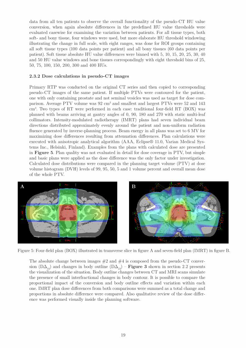
The distance from the isocenter or the centre of the slice to the simulated body contour (r-difference) was measured, as it is an important factor in RTP. Example of the measurements is shown in Figure 6. As the structure is symmetric, the measured distances were averaged for each point with identical theoretical distances - opposing corners of the phantom for
21
example. Theoretical distances were calculated from the position of the corner and the center with the known dimensions of the Duplo-brick – 63.8 mm, 31.8 mm and 19.0 mm in length, wide and height, respectively. These theoretical values were then compared to measured ones.
Figure 6: Data collection measurements in all planes at the isocenter- A: transverse, B: sagittal and C: coronal.
2.4.2 Automated method with grid phantom
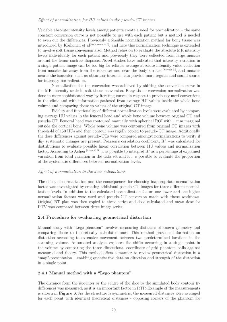
The manual method presented in previous section can reveal an overall view on the distor-tion but do not reveal the detailed, localized characteristics of the geometric distortion. A grid phantom with explicitly differentiated points and automated software based measure-ments can provide more accurate distortion analysis, even beyond the resolution limit. A plastic grid phantom with MRI-visible (liquid-filled) spheres of 10 mm diameter and distributed with 25 mm distance between each sphere was scanned (1.5 T imager Phil-ips Ingenia) with two clinically available sequences: T2-weighted turbo spin echo sequence, universally used for pelvic cancer patients, and in-phase which is Philips’ proprietary in phase - out of phase-based protocol. Pseudo-CT creation is based on this study on in-phase series so distortion analysis was only focused on these images. For T2-sequence, the original clinical protocol was used and field of view (FOV) was increased (500 x 500 x 180 mm) so it would include the exterior contour with even the largest patients. The voxel size was reduced to 1 x 1 x 2 mm. Repetition time (TR) varied between 3000 – 50 000 ms in the protocol, on these scans it was 9.3 seconds, and echo time (TE) between 100 – 120 ms. The default frequency encoding direction was anterior-posterior (AP) and phase encoding occurred in right-left (RL) direction. The same FOV and voxel sizes were selected for in-phase series with dual TE (4.6 and 2.3 ms) for obtaining both In-phase and Out-of-phase images, respectively. Default val-ues for these in the manufacturer’s protocol were 4.0 and 1.8 ms, but the formerly described was used as they have been successfully used previously in HUCH pseudo-CT study made by Korhonen et al. TR was kept at the default value of 6.6 ms. With in-phase series fre-quency direction was RL and phase-encoding was done in AP direction.
22
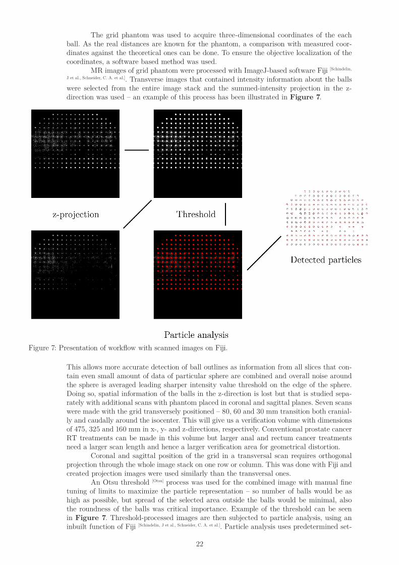
The grid phantom was used to acquire three-dimensional coordinates of the each ball. As the real distances are known for the phantom, a comparison with measured coor-dinates against the theoretical ones can be done. To ensure the objective localization of the coordinates, a software based method was used. MR images of grid phantom were processed with ImageJ-based software Fiji [Schindelin,
J et al., Schneider, C. A. et al.]. Transverse images that contained intensity information about the balls were selected from the entire image stack and the summed-intensity projection in the z-direction was used – an example of this process has been illustrated in Figure 7.
Figure 7: Presentation of workflow with scanned images on Fiji.
This allows more accurate detection of ball outlines as information from all slices that con-tain even small amount of data of particular sphere are combined and overall noise around the sphere is averaged leading sharper intensity value threshold on the edge of the sphere. Doing so, spatial information of the balls in the z-direction is lost but that is studied sepa-rately with additional scans with phantom placed in coronal and sagittal planes. Seven scans were made with the grid transversely positioned – 80, 60 and 30 mm transition both cranial-ly and caudally around the isocenter. This will give us a verification volume with dimensions of 475, 325 and 160 mm in x-, y- and z-directions, respectively. Conventional prostate cancer RT treatments can be made in this volume but larger anal and rectum cancer treatments need a larger scan length and hence a larger verification area for geometrical distortion. Coronal and sagittal position of the grid in a transversal scan requires orthogonal projection through the whole image stack on one row or column. This was done with Fiji and created projection images were used similarly than the transversal ones. An Otsu threshold [Otsu] process was used for the combined image with manual fine tuning of limits to maximize the particle representation – so number of balls would be as high as possible, but spread of the selected area outside the balls would be minimal, also the roundness of the balls was critical importance. Example of the threshold can be seen in Figure 7. Threshold-processed images are then subjected to particle analysis, using an inbuilt function of Fiji [Schindelin, J et al., Schneider, C. A. et al.]. Particle analysis uses predetermined set-
23
tings for contouring areas from the threshold image. Limits for area was set to 10 – 100 mm2 as the theoretical value for sphere with diameter 10 mm is 79 mm2. Roundness values were set to 0.20 – 1.00 (1.00 being perfect circle) for including maximum number of balls but still excluding the most skewed ones – example image can be seen in Figure 7. From these contoured particles, the software is able to calculate the x- and y-coordinates for the centre of each ball. This is done by averaging coordinates of each pixel inside the contour so the variation on the boundary has small effect compared to vast number of pixels in the main part of the ball. Fiji gives an output of x- and y-coordinates as a table file and this data is further analyzed in Excel and R. The origin of the grid was manually placed at the central sphere of the phantom as Fiji outputs all coordinates as positive values (starting from the top left corner of the image window). This is done by translation of the coordinate values – the absolute values of the origin ball are subtracted from each ball thus giving coordinate values around zero both in x- and y-axis, resulting a position of (0, 0) for the origin ball. These values can be then compared to theoretical values calculated from grids known geometry.
2.5 Preliminary tests to adopt HU conversion technique with different sequen-ces and in various body parts
Evaluation of the possibility for exploiting the method with other scanners and sequences was made. As the dual model HU conversion is a robust technique only relying on the abso-lute values of the MR images, pseudo-CT image generation reproduction is also possible with other equipment and software. Yet, before utilizing the process, gathering of average values from a patient group broad enough is a necessity. Additional bone contouring is also needed but that can be done manually if no other means are available. Initial test conversion was made for T2-weighted MR images (1.5 T Philips Ingenia and 1.5 T GE Optima MR450w scanners) with the same ROI-based method – collecting appropriate number of data points from soft tissue and bone segment from the original MR images. HU values were not collected separately, but previously used values from in-phase conversion were used as they are standard and calibrated against same constraints – water = 0 HUs and air = -1000 HUs – so we can presume their values are unchanged in different conversion curves. T2-weighted sequence was tested for pelvis and thigh and in-phase images were additionally applied for abdomen. These test pseudo-CT conversions were made only with single example.

24
Results
3.1 Updated dual model HU conversion technique
Overall results from data collection can be seen in Figure 8 – all 1600 data points from ten patients in the same graph. It is easy to see a clear need for the dual model conversion method, as the overlapping is present nearly at full scale – urine and parts of cortical bone with muscle tissue and dense spongy bone overlapping in the intensity scale.
Figure 8: Collected data points plotted as HU values against MR image intensity values.
0 200 400 600 800 1000 1200 1400
0
500
1000
1500
Urine Muscle Visceral fat Subcutaneous fat Prostate Rectal wall Cortical bone Dense spongy bone Low density spongy bone Bone marrow
MR image intensity value
CT
imag
e H
U v
alue
3.1.1 Conversion curve for soft tissue
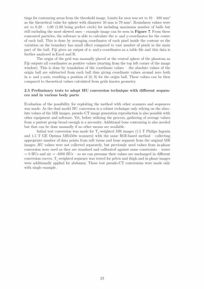
Conversion model was reconstructed of average values of CT image intensities for urine, muscle and subcutaneous fat for assignment HU values. Step locations were selected using average values and SDs in MRI image intensities for ROI groups of same tissues. Figure 9 presents the conversion curve and tissue type specific data points as the conversion steps – before and after the update. For example mean CT image HU value for urine was 12 and for MRI image 191 with SD of 35 – resulting a bulk HU value assignment of 12 for MRI intensity values smaller than intensity of 226. Conversion between the bulk HU values was done with linear interpolation. Image contains also the old conversion curve before the scanner update – it is clear that pseudo-CT conversion based on the old MRI intensities would not have resulted as successful HU value presentation of the patient. Comparing step positions against old conversion values, an average increase of 1.92 can be seen – with individual relations of step threshold changes: urine upper limit change of 2.09 when comparing previous model, lower muscle step 1.77, upper muscle step 1.94 and lower fat 1.89. When comparing data points among ten cases a clear shift in MR image intensity can be seen and this is compensated by normalization e.g. using the conversion curve with best fit among ten predetermined normalized conversion models. Figure 10 illustrates all soft tissue data collection points patientwise. AssessmentROIs capture this intensity variation in more precise manner as there are voxels recorded also on the tissue boundaries, containing partly both tissues inside 5 mm diameter ROI, which results in more data points in the region between muscle and adipose tissue. Figure 11 provides a good example with three patients around the scale.
25
100 200 300 400 500 600 700 800 900 1000 1100
-100
-50
0
50
Urine Muscle Visceral fat Subcutaneous fat Prostate Rectal wall
CT
imag
e H
U v
alue
MR image intensity value
8
55
-104
12
45
-98
112 150 212 346
234 265 412 654
Soft tissue conversion model
old border values new border values
Figure 10: Data collection points for all ten data group patients individually labeled by different colors.
100 200 300 400 500 600 700 800 900 1000 1100 1200
-100
-50
0
50
Patient IDs PD6 PD3 PD4 PD5 PD2 PD1 PD10 PD7 PD9 PD8
CT
imag
e H
U v
alue
MR image intensity value
Figure 9: Soft tissue conversion curves generated with average and SD data from MR images with bulk HU values calculated from original CT images – before and after the MR scanner update.

26
3.1.2 Conversion curve for bone segments
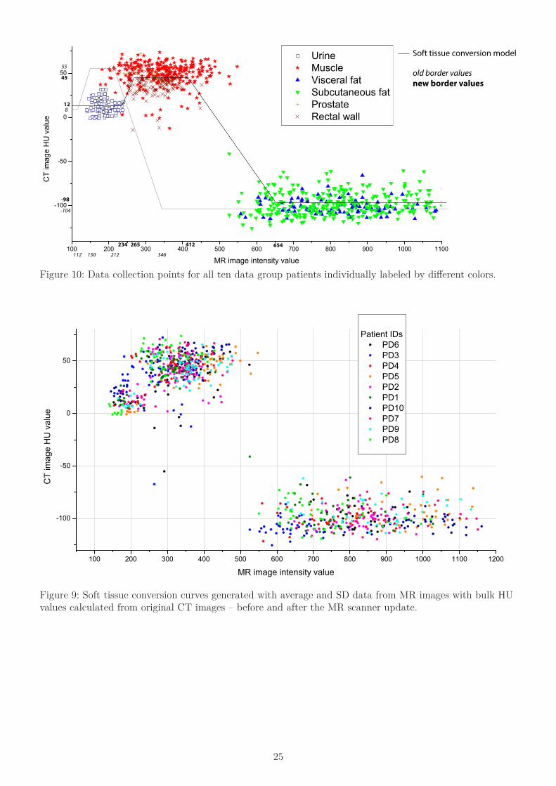
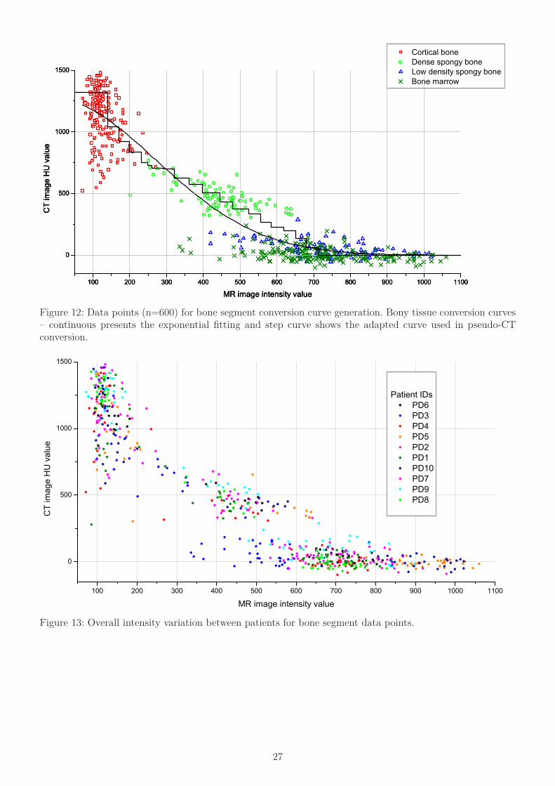
MR image intensity values ranged from 93 to 163 (one sigma SD) in cortical bone and correspondingly between 873-1355 HUs in CT images. Average HU value for bone marrow was 15±63 with MR intensity values of 721±142. For dense spongy bone and low density spongy bone average HU values for data collection ROIs were 473±106 and 57±80, re-spectively, and corresponding MR image intensity values ranged at 349-553 and 599-865, respectively. By comparing MR image intensity values before and after scanner update for cortical bone, bone marrow, dense spongy bone and low density spongy bone, an average relative increase was 1.24, 1.72, 1.94 and 2.06 times higher than before update, respectively. Absolute averages of each tissue type were not used for conversion model generation as in soft tissue case, but a three variable exponential (ea+bx+cx2) fitting was done for all data points. This continuous conversion curve was divided to 20 intensity ranges, as had been previously done for workflows before the update [Korhonen et al.3]. Ranges were then addition-ally shifted manually according to the fitted exponential, the distribution of data points in particular range and also the earlier clinical conversion curves, resulting more accurate and versatile conversion curve for all normalization factors. A strong divergence in the MR intensity values can be found between patients, similarly to the soft tissue intensity values. This results in a requirement of normalization also for bony tissue conversion – in the clinical workflow both tissue normalizations are merged in to a single conversion workflow for particular intensity range. Figure 12 pres-ents four different bone tissue types with continuous exponential fitting and step instance conversation curve of the average normalization. Figure 13 visualizes the absolute MR intensity value fluctuation between patients for bony tissue.
Figure 11: AssessmentROIs for three patients to visualize the variation in the absolute intensity values among different patients. Coil bridge sizes (small, medium and large) used for each patient mentioned – for patient 3 two different size coil bridge were used. Small coil bridges are used for smaller patients, resulting higher intensity values because of smaller patient volume and shorter voxel to coil distance.
100 200 300 400 500 600 700 800 900 1000 1100 1200
-100
-50
0
50 Assesment ROIs patient 3 - M caud., L cran. Assesment ROIs patient 4 - L Assesment ROIs patient 6 - S
CT
imag
e H
U v
alue
MR image intensity value
27
100 200 300 400 500 600 700 800 900 1000 1100
0
500
1000
1500
Cortical bone Dense spongy bone Low density spongy bone Bone marrow
CT
imag
e H
U v
alue
MR image intensity value100 200 300 400 500 600 700 800 900 1000 1100
0
500
1000
1500
CT
imag
e H
U v
alue
MR image intensity value100 200 300 400 500 600 700 800 900 1000 1100
0
500
1000
1500
CT
imag
e H
U v
alue
MR image intensity value
Figure 12: Data points (n=600) for bone segment conversion curve generation. Bony tissue conversion curves – continuous presents the exponential fitting and step curve shows the adapted curve used in pseudo-CT conversion.
100 200 300 400 500 600 700 800 900 1000 1100
0
500
1000
1500
Patient IDs PD6 PD3 PD4 PD5 PD2 PD1 PD10 PD7 PD9 PD8
CT
imag
e H
U v
alue
MR image intensity value
Figure 13: Overall intensity variation between patients for bone segment data points.
28
3.2 Example of the pseudo-CT image generation
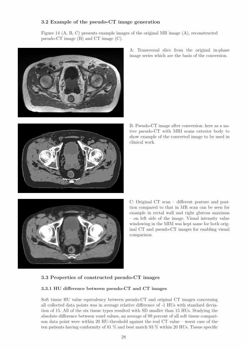
Figure 14 (A, B, C) presents example images of the original MR image (A), reconstructed pseudo-CT image (B) and CT image (C).
A: Transversal slice from the original in-phase image series which are the basis of the conversion.
B: Pseudo-CT image after conversion: here as a na-tive pseudo-CT with MRI scans exterior body to show example of the converted image to be used in clinical work.
C: Original CT scan – different posture and posi-tion compared to that in MR scan can be seen for example in rectal wall and right gluteus maximus – on left side of the image. Visual intensity value windowing in the MIM was kept same for both orig-inal CT and pseudo-CT images for enabling visual comparison.
3.3 Properties of constructed pseudo-CT images
3.3.1 HU difference between pseudo-CT and CT images
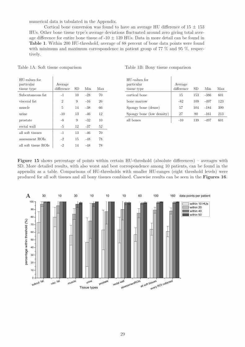
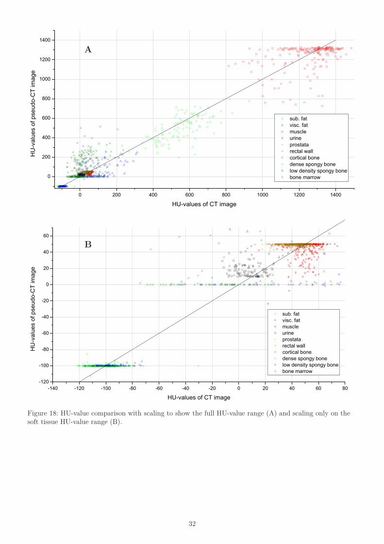
Soft tissue HU value equivalency between pseudo-CT and original CT images concerning all collected data points was in average relative difference of -1 HUs with standard devia-tion of 15. All of the six tissue types resulted with SD smaller than 15 HUs. Studying the absolute difference between voxel values, an average of 89 percent of all soft tissue compari-son data point were within 20 HU-threshold against the real CT value – worst case of the ten patients having conformity of 81 % and best match 93 % within 20 HUs. Tissue specific
29
numerical data is tabulated in the Appendix. Cortical bone conversion was found to have an average HU difference of 15 ± 153 HUs. Other bone tissue type’s average deviations fluctuated around zero giving total aver-age difference for entire bone tissue of -10 ± 139 HUs. Data in more detail can be found in Table 1. Within 200 HU-threshold, average of 88 percent of bone data points were found with minimum and maximum correspondence in patient group of 77 % and 95 %, respec-tively.
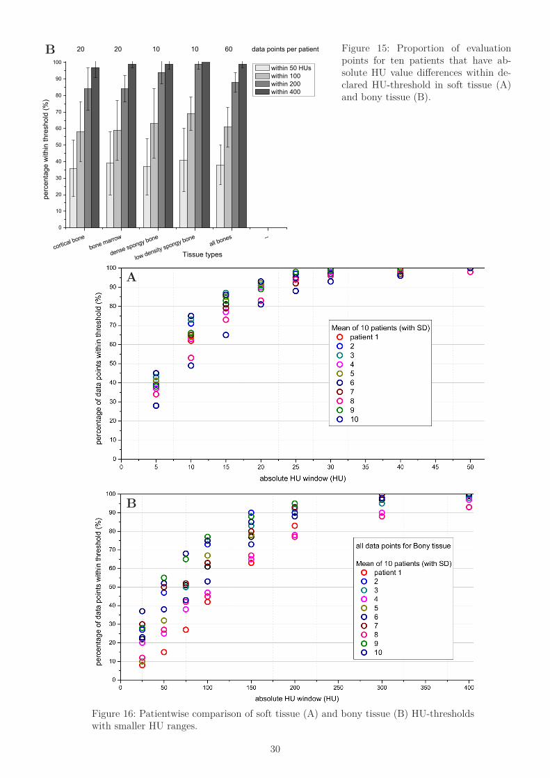
Figure 15 shows percentage of points within certain HU-threshold (absolute differences) – averages with SD. More detailed results, with also worst and best correspondence among 10 patients, can be found in the appendix as a table. Comparisons of HU-thresholds with smaller HU-ranges (eight threshold levels) were produced for all soft tissues and all bony tissues combined. Casewise results can be seen in the Figures 16.
HU-values for particular tissue type
Average difference SD Min Max
Subcutaneous fat -1 10 -28 70visceral fat 2 9 -16 26muscle 5 14 -38 66urine -10 13 -46 12prostate -8 9 -32 10rectal wall -5 12 -37 52all soft tissues -1 13 -46 70assessment ROIs -2 15 -48 78all soft tissue ROIs -2 14 -48 78
Table 1A: Soft tissue comparison
HU-values for particular tissue type
Average difference SD Min Max
cortical bone 15 153 -386 601bone marrow -82 109 -497 123Spongy bone (dense) 57 104 -184 399Spongy bone (low density) 27 80 -161 213all bones -10 139 -497 601
Table 1B: Bony tissue comparison
subcut. fatvisc. fat
muscle urineprostate
rectal wall
assessmentROIs
all soft tissues
every ROI collected0
10
20
30
40
50
60
70
80
90
100
perc
enta
ge w
ithin
thre
shol
d (%
)
Tissue types
within 10 HUs within 20 within 40 within 50
30 10 30 10 10 10 60 100 160 data points per patientA
30
cortical bone
bone marrow
dense spongy bone
low density spongy boneall bones --
0
10
20
30
40
50
60
70
80
90
100
perc
enta
ge w
ithin
thre
shol
d (%
)
Tissue types
within 50 HUs within 100 within 200 within 400
20 20 10 10 60 data points per patient Figure 15: Proportion of evaluation points for ten patients that have ab-solute HU value differences within de-clared HU-threshold in soft tissue (A) and bony tissue (B).
B
Figure 16: Patientwise comparison of soft tissue (A) and bony tissue (B) HU-thresholds with smaller HU ranges.
B
A
31
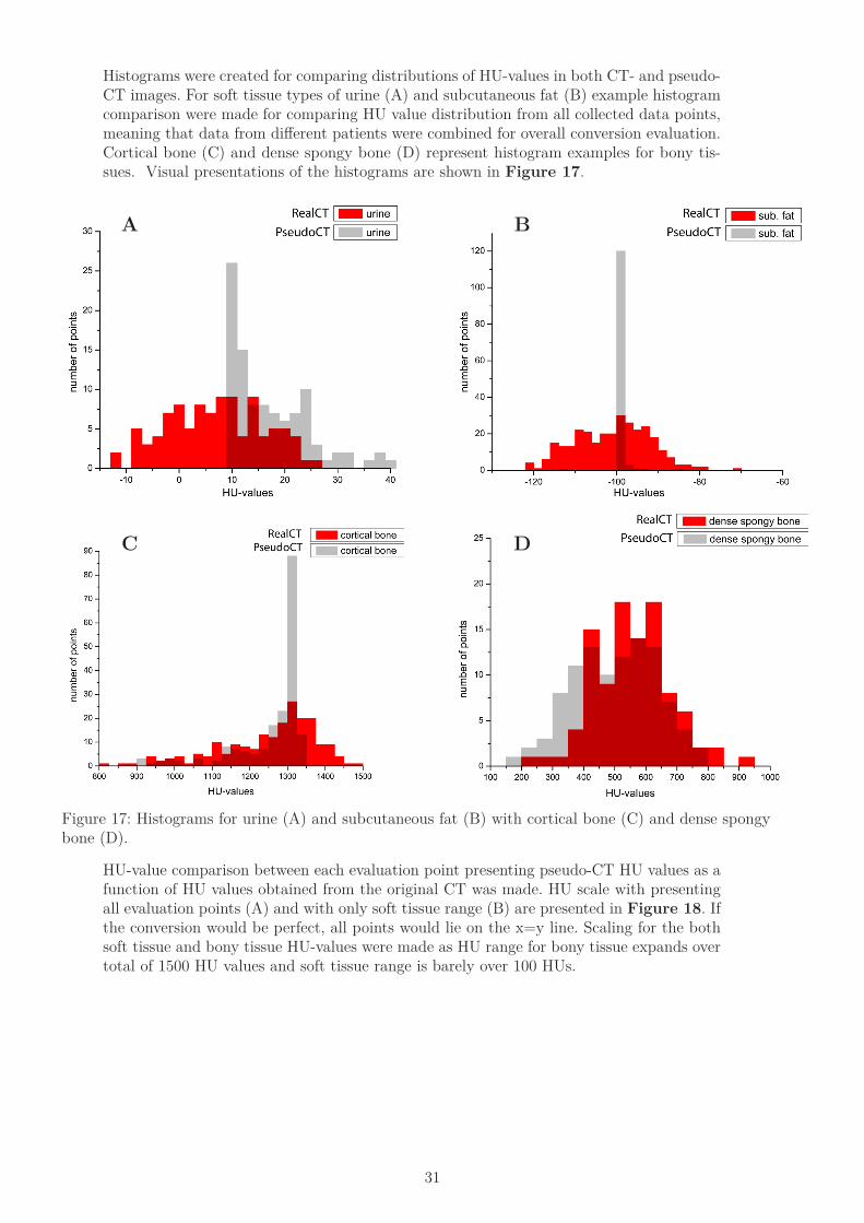
Histograms were created for comparing distributions of HU-values in both CT- and pseudo-CT images. For soft tissue types of urine (A) and subcutaneous fat (B) example histogram comparison were made for comparing HU value distribution from all collected data points, meaning that data from different patients were combined for overall conversion evaluation. Cortical bone (C) and dense spongy bone (D) represent histogram examples for bony tis-sues. Visual presentations of the histograms are shown in Figure 17.
Figure 17: Histograms for urine (A) and subcutaneous fat (B) with cortical bone (C) and dense spongy bone (D).
HU-value comparison between each evaluation point presenting pseudo-CT HU values as a function of HU values obtained from the original CT was made. HU scale with presenting all evaluation points (A) and with only soft tissue range (B) are presented in Figure 18. If the conversion would be perfect, all points would lie on the x=y line. Scaling for the both soft tissue and bony tissue HU-values were made as HU range for bony tissue expands over total of 1500 HU values and soft tissue range is barely over 100 HUs.
BA
C D
32
Figure 18: HU-value comparison with scaling to show the full HU-value range (A) and scaling only on the soft tissue HU-value range (B).
0 200 400 600 800 1000 1200 1400
0
200
400
600
800
1000
1200
1400
sub. fat visc. fat muscle urine prostata rectal wall cortical bone dense spongy bone low density spongy bone bone marrow
HU
-val
ues
of p
seud
o-C
T im
age
HU-values of CT image
-140 -120 -100 -80 -60 -40 -20 0 20 40 60 80-120
-100
-80
-60
-40
-20
0
20
40
60
sub. fat visc. fat muscle urine prostata rectal wall cortical bone dense spongy bone low density spongy bone bone marrow
HU
-val
ues
of p
seud
o-C
T im
age
HU-values of CT image
B
A
33
3.3.2 Dose distribution in pseudo-CT images
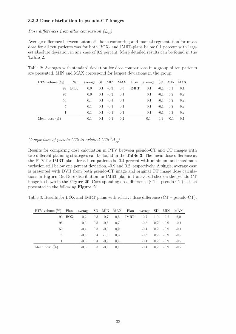
Dose differences from atlas comparison (Δ12)
Average difference between automatic bone contouring and manual segmentation for mean dose for all ten patients was for both BOX- and IMRT-plans below 0.1 percent with larg-est absolute deviation in any case of 0.2 percent. More detailed results can be found in the Table 2.
Table 2: Averages with standard deviation for dose comparisons in a group of ten patients are presented. MIN and MAX correspond for largest deviations in the group.
Comparison of pseudo-CTs to original CTs (Δ34)
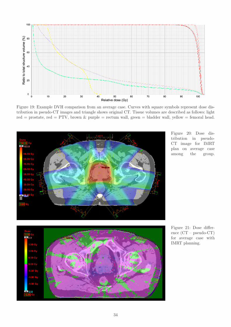
Results for comparing dose calculation in PTV between pseudo-CT and CT images with two different planning strategies can be found in the Table 3. The mean dose difference at the PTV for IMRT plans for all ten patients is -0.4 percent with minimum and maximum variation still below one percent deviation, -0.9 and 0.2, respectively. A single, average case is presented with DVH from both pseudo-CT image and original CT image dose calcula-tions in Figure 19. Dose distribution for IMRT plan in transversal slice on the pseudo-CT image is shown in the Figure 20. Corresponding dose difference (CT – pseudo-CT) is then presented in the following Figure 21.
Table 3: Results for BOX and IMRT plans with relative dose difference (CT – pseudo-CT).
PTV volume (%) Plan average SD MIN MAX Plan average SD MIN MAX99 BOX 0,0 0,1 -0,2 0,0 IMRT 0,1 -0,1 0,1 0,195 0,0 0,1 -0,2 0,1 0,1 -0,1 0,2 0,250 0,1 0,1 -0,1 0,1 0,1 -0,1 0,2 0,25 0,1 0,1 -0,1 0,1 0,1 -0,1 0,2 0,21 0,1 0,1 -0,1 0,1 0,1 -0,1 0,2 0,2
Mean dose (%) 0,1 0,1 -0,1 0,2 0,1 0,1 -0,1 0,1
PTV volume (%) Plan average SD MIN MAX Plan average SD MIN MAX99 BOX -0,2 0,3 -0,7 0,5 IMRT -0,7 1,0 -2,2 2,095 -0,3 0,3 -0,6 0,7 -0,5 0,2 -0,9 -0,150 -0,4 0,3 -0,9 0,2 -0,4 0,2 -0,9 -0,15 -0,3 0,4 -1,0 0,3 -0,3 0,2 -0,9 -0,21 -0,3 0,4 -0,9 0,4 -0,4 0,2 -0,9 -0,2
Mean dose (%) -0,3 0,3 -0,9 0,1 -0,4 0,2 -0,9 -0,2
34
Figure 19: Example DVH comparison from an average case. Curves with square symbols represent dose dis-tribution in pseudo-CT images and triangle shows original CT. Tissue volumes are described as follows: light red = prostate, red = PTV, brown & purple = rectum wall, green = bladder wall, yellow = femoral head.
Figure 20: Dose dis-tribution in pseudo-CT image for IMRT plan on average case among the group.
Figure 21: Dose differ-ence (CT – pseudo-CT) for average case with IMRT planning.

35
Effect of the body outline changes to dose calculations (Δ24)
Table 4 presents the proportional dose differences caused by body outline changes and pseudo-CT image conversion. Proportion between the two effects is presented in percent of the total absolute change between native pseudo-CT (with MR body contour) and original CT image. Body effect represents the dose difference between images #2 and #3. Pseudo effect is the dose difference caused HU conversion, see Figure 3.
Table 4: Proportions of body outline and pseudo conversion effects for different relative volumes of PTV and for the mean dose.
The mean dose difference between images 2 and 3 was 0.16 percent and between 3 and 4 -0.40 percent – absolute change being 0.55 percent – resulting to 28 % contribution for the body contour change between scans. More importantly, the standard deviation for the 10 patient groups for both dose difference groups could be compared. Pseudo-CT and CT comparison led to SD of 0.19 percent within a ten patient group when body contour changes correspond to almost a double of larger variation of SD 0.36 percent.
Comparing water and homogeneous models against pseudo-CT dose calculations
Dose comparison results can be found in the Table 5. For IMRT plans the standard de-viation for mean PTV dose differences between the original CT and the reference pseudo was 1.0, 0.7 and 0.2 percent for Water, Dual homogeneous and pseudo-CT, respectively. When comparing ten patient’s dose differences between Water and pseudo-CT, F-test gives results of p=0.0001 for clearly indicating a significantly smaller variation for pseudo-CT images. Dual homogeneous model operates better when comparing to Water images as it has F-test p-value of 0.0014, but the variation between patients is still larger than with pseudo-CT conversion.
Table 5: Dose comparison results for both planning strategies with average difference in a ten patient group, standard deviation with minimum and maximum deviation. All values in percentage.
Proportion of each effect (%)
Plan PTV volume (%)
Total absolute
change (%) body effect Pseudo effectIMRT 99 0,81 19 81
95 0,67 22 7850 0,54 26 745 0,59 41 591 0,72 49 51
Mean dose (%) 0,55 28 72
Mean PTV Dose difference between: average SD Min Max
BOX CT vs. Pseudo-CT -0.3 0.3 -0.9 0.1CT vs. Dual homogeneous 0.9 0.9 -0.2 2.5
CT vs. Water -2.3 1.0 -3.4 -0.4IMRT CT vs. Pseudo-CT -0.4 0.2 -0.9 -0.2
CT vs. Dual homogeneous 0.3 0.7 -0.7 1.5CT vs. Water -1.8 1.0 -3.7 -0.4
36
3.3.3.1 Effect of normalization for HU values in the pseudo-CT images
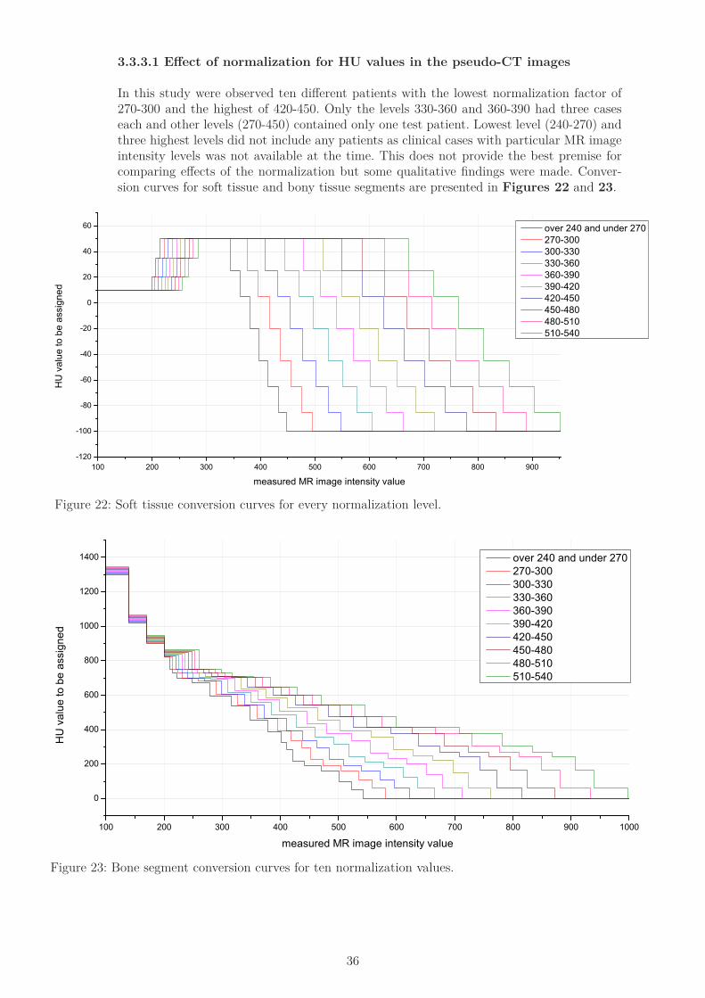
In this study were observed ten different patients with the lowest normalization factor of 270-300 and the highest of 420-450. Only the levels 330-360 and 360-390 had three cases each and other levels (270-450) contained only one test patient. Lowest level (240-270) and three highest levels did not include any patients as clinical cases with particular MR image intensity levels was not available at the time. This does not provide the best premise for comparing effects of the normalization but some qualitative findings were made. Conver-sion curves for soft tissue and bony tissue segments are presented in Figures 22 and 23.
100 200 300 400 500 600 700 800 900-120
-100
-80
-60
-40
-20
0
20
40
60
HU
val
ue to
be
assi
gned
measured MR image intensity value
over 240 and under 270 270-300 300-330 330-360 360-390 390-420 420-450 450-480 480-510 510-540
Figure 22: Soft tissue conversion curves for every normalization level.
Figure 23: Bone segment conversion curves for ten normalization values.
100 200 300 400 500 600 700 800 900 1000
0
200
400
600
800
1000
1200
1400
HU
val
ue to
be
assi
gned
measured MR image intensity value
over 240 and under 270 270-300 300-330 330-360 360-390 390-420 420-450 450-480 480-510 510-540
37
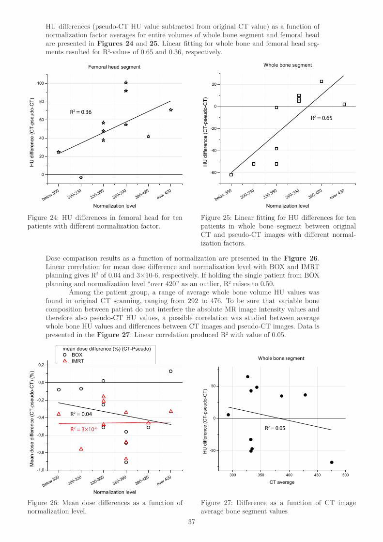
HU differences (pseudo-CT HU value subtracted from original CT value) as a function of normalization factor averages for entire volumes of whole bone segment and femoral head are presented in Figures 24 and 25. Linear fitting for whole bone and femoral head seg-ments resulted for R2-values of 0.65 and 0.36, respectively.
Figure 24: HU differences in femoral head for ten patients with different normalization factor.
Figure 25: Linear fitting for HU differences for ten patients in whole bone segment between original CT and pseudo-CT images with different normal-ization factors.
Figure 26: Mean dose differences as a function of normalization level.
Figure 27: Difference as a function of CT image average bone segment values
Dose comparison results as a function of normalization are presented in the Figure 26. Linear correlation for mean dose difference and normalization level with BOX and IMRT planning gives R2 of 0.04 and 3×10⁻⁶, respectively. If holding the single patient from BOX planning and normalization level “over 420” as an outlier, R2 raises to 0.50. Among the patient group, a range of average whole bone volume HU values was found in original CT scanning, ranging from 292 to 476. To be sure that variable bone composition between patient do not interfere the absolute MR image intensity values and therefore also pseudo-CT HU values, a possible correlation was studied between average whole bone HU values and differences between CT images and pseudo-CT images. Data is presented in the Figure 27. Linear correlation produced R2 with value of 0.05.
below 300300-330
330-360360-390
390-420over 420
0
20
40
60
80
100
Femoral head segment
HU
diff
eren
ce (C
T-ps
eudo
-CT)
Normalization level
R2 = 0.36
below 300300-330
330-360360-390
390-420over 420
-60
-40
-20
0
20
HU
diff
eren
ce (C
T-ps
eudo
-CT)
Normalization level
Whole bone segment
R2 = 0.65
below 300300-330
330-360360-390
390-420over 420
-1,0
-0,8
-0,6
-0,4
-0,2
0,0
0,2
BOX IMRT
Mea
n do
se d
iffer
ence
(CT-
pseu
do-C
T) (%
)
Normalization level
R2 = 0.04
R2 = 3×10⁻⁶
mean dose difference (%) (CT-Pseudo)
300 350 400 450 500
-50
0
50
HU
diff
eren
ce (C
T-ps
eudo
-CT)
CT average
R2 = 0.05
Whole bone segment
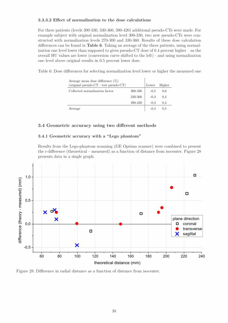
38
3.3.3.2 Effect of normalization to the dose calculations
For three patients (levels 300-330, 330-360, 390-420) additional pseudo-CTs were made. For example subject with original normalization level 300-330, two new pseudo-CTs were con-structed with normalization levels 270-300 and 330-360. Results of these dose calculation differences can be found in Table 6. Taking an average of the three patients, using normal-ization one level lower than supposed to gives pseudo-CT dose of 0.4 percent higher – as the overall HU values are lower (conversion curve shifted to the left) - and using normalization one level above original results in 0.5 percent lower dose.
Table 6: Dose differences for selecting normalization level lower or higher the measured one
Average mean dose difference (%) (original pseudo-CT - test pseudo-CT) Lower HigherCollected normalization factor 300-330 -0,5 0,6
330-360 -0,4 0,4390-420 -0,3 0,4
Average -0,4 0,5
3.4 Geometric accuracy using two different methods
3.4.1 Geometric accuracy with a “Lego phantom”
Results from the Lego-phantom scanning (GE Optima scanner) were combined to present the r-difference (theoretical – measured) as a function of distance from isocenter. Figure 28 presents data in a single graph.
Figure 28: Difference in radial distance as a function of distance from isocenter.
60 80 100 120 140 160 180 200 220 240
-0,5
0,0
0,5
1,0
plane direction coronal transverse sagittal
diffe
renc
e (th
eory
- m
easu
red)
(mm
)
theoretical distance (mm)
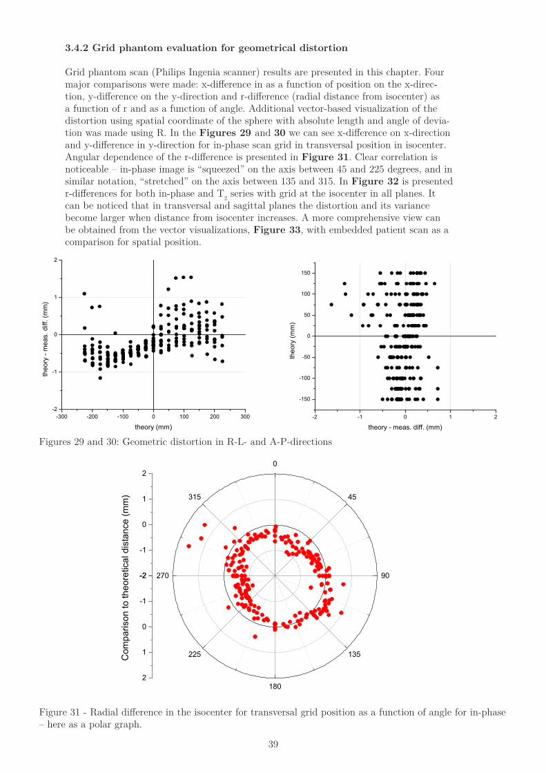
39
3.4.2 Grid phantom evaluation for geometrical distortion
Grid phantom scan (Philips Ingenia scanner) results are presented in this chapter. Four major comparisons were made: x-difference in as a function of position on the x-direc-tion, y-difference on the y-direction and r-difference (radial distance from isocenter) as a function of r and as a function of angle. Additional vector-based visualization of the distortion using spatial coordinate of the sphere with absolute length and angle of devia-tion was made using R. In the Figures 29 and 30 we can see x-difference on x-direction and y-difference in y-direction for in-phase scan grid in transversal position in isocenter. Angular dependence of the r-difference is presented in Figure 31. Clear correlation is noticeable – in-phase image is “squeezed” on the axis between 45 and 225 degrees, and in similar notation, “stretched” on the axis between 135 and 315. In Figure 32 is presented r-differences for both in-phase and T2 series with grid at the isocenter in all planes. It can be noticed that in transversal and sagittal planes the distortion and its variance become larger when distance from isocenter increases. A more comprehensive view can be obtained from the vector visualizations, Figure 33, with embedded patient scan as a comparison for spatial position.
Figures 29 and 30: Geometric distortion in R-L- and A-P-directions
Figure 31 - Radial difference in the isocenter for transversal grid position as a function of angle for in-phase – here as a polar graph.
-300 -200 -100 0 100 200 300-2
-1
0
1
2
theo
ry -
mea
s. d
iff. (
mm
)
theory (mm)-2 -1 0 1 2
-150
-100
-50
0
50
100
150
theo
ry (m
m)
theory - meas. diff. (mm)
-2
-1
0
1
20
45
90
135
180
225
270
315
-2
-1
0
1
2
Com
paris
on to
theo
retic
al d
ista
nce
(mm
)
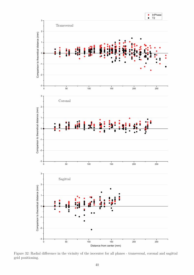
40
Figure 32: Radial difference in the vicinity of the isocenter for all planes - transversal, coronal and sagittal grid positioning.
Coronal
Sagittal
Transversal
0 50 100 150 200 250-3
-2
-1
0
1
2
3
InPhase T2
Com
paris
on to
theo
retic
al d
ista
nce
(mm
)
0 50 100 150 200 250-3
-2
-1
0
1
2
3
Com
paris
on to
theo
retic
al d
ista
nce
(mm
)
0 50 100 150 200 250-3
-2
-1
0
1
2
3
Com
paris
on to
theo
retic
al d
ista
nce
(mm
)
Distance from center (mm)
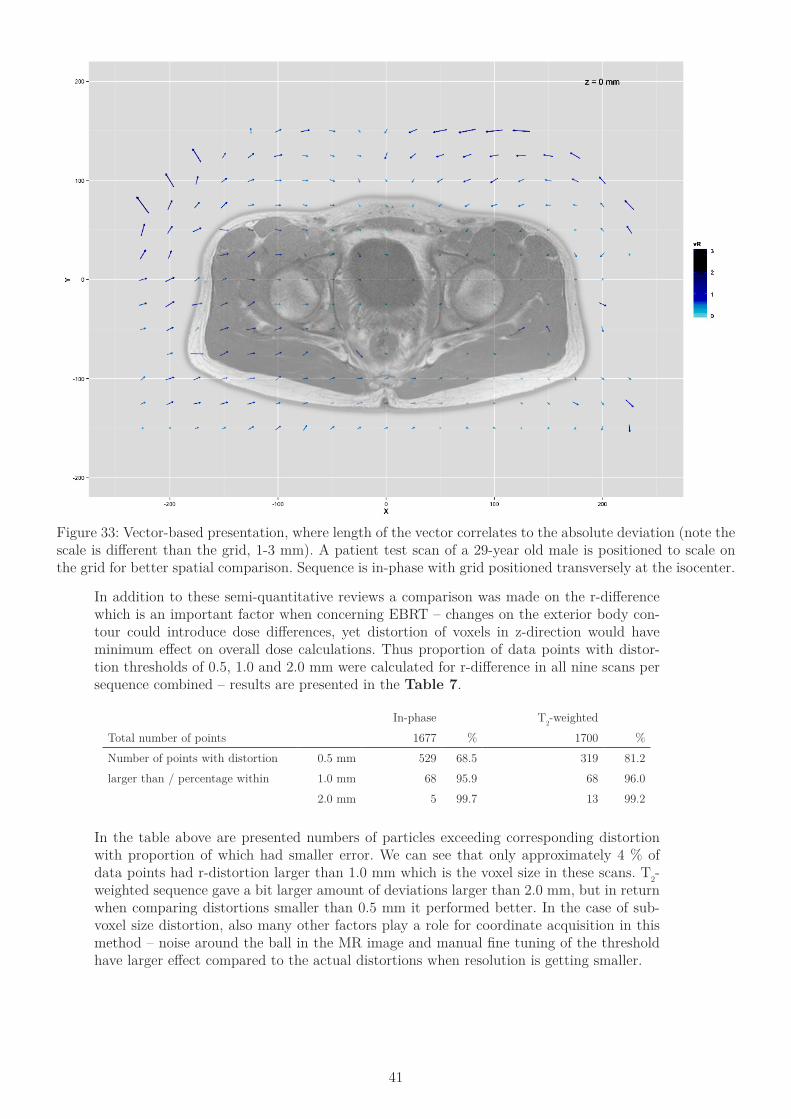
41
Figure 33: Vector-based presentation, where length of the vector correlates to the absolute deviation (note the scale is different than the grid, 1-3 mm). A patient test scan of a 29-year old male is positioned to scale on the grid for better spatial comparison. Sequence is in-phase with grid positioned transversely at the isocenter.
In addition to these semi-quantitative reviews a comparison was made on the r-difference which is an important factor when concerning EBRT – changes on the exterior body con-tour could introduce dose differences, yet distortion of voxels in z-direction would have minimum effect on overall dose calculations. Thus proportion of data points with distor-tion thresholds of 0.5, 1.0 and 2.0 mm were calculated for r-difference in all nine scans per sequence combined – results are presented in the Table 7.
In-phase T2-weightedTotal number of points 1677 % 1700 %Number of points with distortion 0.5 mm 529 68.5 319 81.2larger than / percentage within 1.0 mm 68 95.9 68 96.0
2.0 mm 5 99.7 13 99.2
In the table above are presented numbers of particles exceeding corresponding distortion with proportion of which had smaller error. We can see that only approximately 4 % of data points had r-distortion larger than 1.0 mm which is the voxel size in these scans. T2-weighted sequence gave a bit larger amount of deviations larger than 2.0 mm, but in return when comparing distortions smaller than 0.5 mm it performed better. In the case of sub-voxel size distortion, also many other factors play a role for coordinate acquisition in this method – noise around the ball in the MR image and manual fine tuning of the threshold have larger effect compared to the actual distortions when resolution is getting smaller.
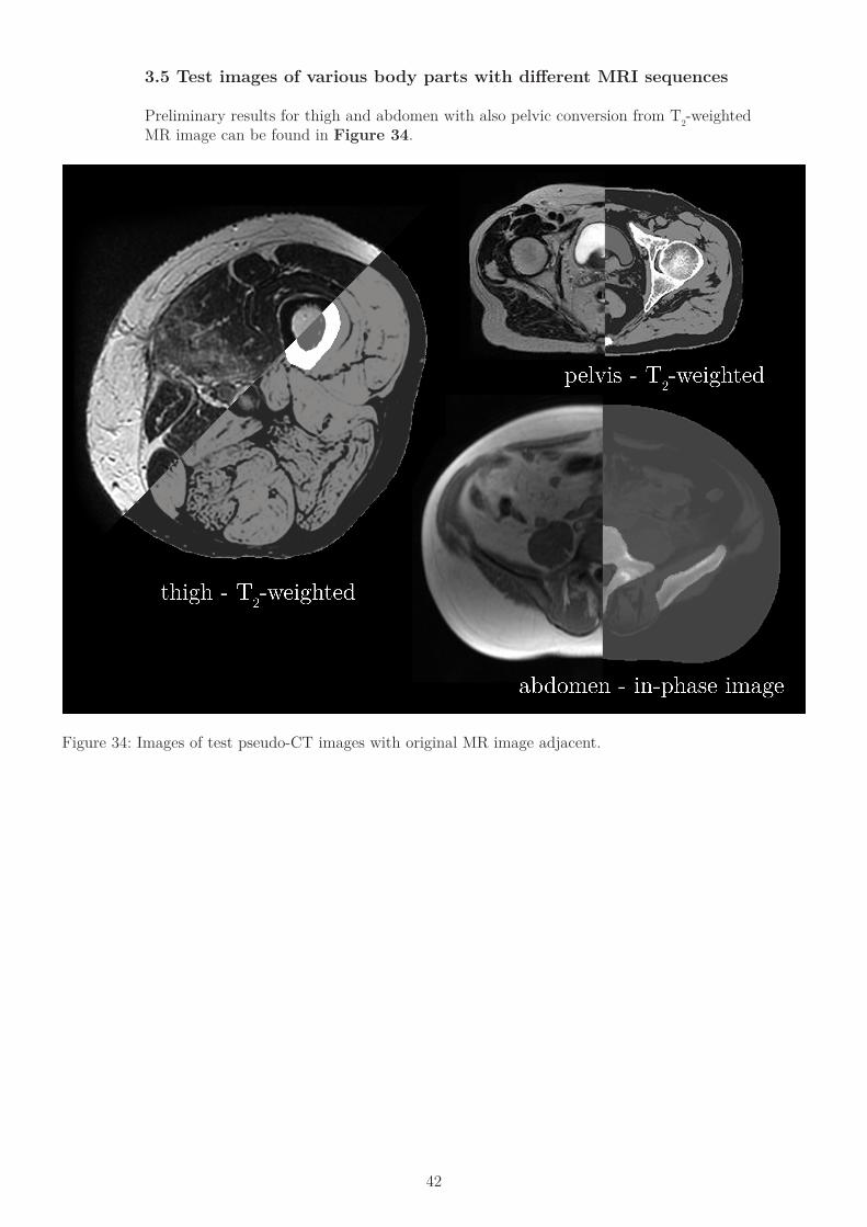
42
3.5 Test images of various body parts with different MRI sequences
Preliminary results for thigh and abdomen with also pelvic conversion from T2-weighted MR image can be found in Figure 34.
Figure 34: Images of test pseudo-CT images with original MR image adjacent.
43
Discussion
4.1 Conversion creation
The presented dual model conversion method provides suffcient HU conversion for radiation therapy purposes. If the step-based conversion curves would be replaced with continuous methods, the average HU values in a certain volume e.g. bone segment or blad-der would change only a minuscule amount, yet more accurate representation of individual voxels with high detail could provide better results for generation of DRRs. Fully continu-ous HU value assigning is not possible with MIM-software, and thus another external soft-ware method would be needed. As the conversion model is tightly knit to the absolute MR image intensity, it is strongly dependent on possible changes in the primary MR images. Artifacts that affect intensity levels may result in a systematic error in pseudo-CT images – as well any artifacts that induce a geometric distortion are exclusive factors for pseudo-CT generation. The same property makes this method robust and conceivable for clinical use – it does not use any pre-clinical sequences and it is mainly intended from MRI scanners used already for RTP simulation, hence verified geometric accuracy and MR compatible immobilization devices are present previously. User dependent ROI-based conversion curve creation workflow is laborious and time consuming. Another possible way to create the conversion curve between MR image intensities and CT image HU values could be to measure only the tissue specific variation from MR scans with volumetric measurements and rely on literature values considering HU values. This could provide better observation for intensity variation in MR images compar-ing to point-to-point method used in this study, and result to more accurate conversion as the full intensity variation in each tissue type is taken to account. Additionally, deformable registration between MR and CT images could permit the use of software for automatic and random selection of ROIs from the patient volume. This approach could provide sta-tistically more powerful conversion curve determination and diminish the effect of intensity value correlation uncertainty between MR and CT scans. MRI-only based RTP cannot replace fully all instances of CT based imaging cases as all patients are not compatible for MR scanning [Harden S. P.] – old pacemakers or prostheses may create a need for conventional CT scan. Procedure length can produce an impediment for some patients, as the CT scan is merely seconds in duration but full MR scan cycle with possibly multiple sequences can last tens of minutes. 4.2 HU-comparison
Soft tissue and bony tissue conversion model produce HU values for pseudo-CT images with good correlation to original CT images with average difference of -1±13 HUs and -10±139 HUs, respectively. Absolute and voxel-to-voxel comparison in HU values is not as important as the average tissue representation for dose calculation purposes. HU value comparison was made in this study with only manually selected ball-ROIs which causes av-eraging and potential subjectivity. To evaluate the genuine HU variation between pseudo-CT and original CT scans, voxel-to-voxel comparison method could provide additional en-hancements. Statistical power and overall evaluation ability would improve significantly as data point quantity per patient rises from scale of hundreds to at least 106. Automated and user-unrelated methods for data collection would permit faster and more adaptable way to examine data. Computational approach would also provide possibility to take account also other characteristics from the voxel based scanning data, such as three dimensional position of each voxel, neighboring voxels’ intensities and possibly intensities of other co-registered image stacks. This would open up a whole new alternative tool box for data evaluation and even pseudo-CT creation using coding platforms such as Matlab or Python-based coding libraries. HU values were studied also qualitatively with histograms presented in section 3.3.1. It is possible to evaluate the characteristics of the both CT and pseudo-CT tissue-specific histograms. The spreading of the HU-values in the CT image is mainly caused by the noise

44
of the measurement itself and heterogeneous composition of adipose tissue containing blood vessels etc. In the original in-phase MR image same heterogeneity can be found but as dur-ing the conversion all voxels with intensity values higher than predetermined threshold are assigned with uniform HU-value produces highly focused distribution of HU-values in the pseudo-CT images for subcutaneous fat with average of -99.8 and standard deviation of 1.3, when in CT image -100.7 and 9.8, respectively. Similar behavior can be found also in other tissue types. In comparison with urine, a one-sided fluctuation in pseudo-CT HU values is present. This is due to characteristics of the conversion – all voxels with intensity lower than threshold for urine are assigned single HU value of 10 and values between 10 and 50 HUs are result of interpolation steps between muscle and urine. Even though the assigned pseudo-CT HU value is set to 10 HUs which is the approximate average for urine in CT images, the resulting average in pseudo-CT images is 17.5 HUs with standard deviation of 7.8 HUs. These effects hold noticeable effects on the HU value spectrum but their impact for dose calculations is minimal as long as tissue-specific HU averages are on the same level in both CT and pseudo-CT images. Comparison between different normalization levels revealed systematic error in the whole bone and femoral head volumes average HU values. With a patient group this small, containing only one patient for in four normalization levels, it is diffcult to deduce a clear reason for this effect but uneven conversion curve generation between different normaliza-tion factors might be the cause. Iteration on the conversion curves generation for bony tissue and larger patient group, or variable intensity scanning with one volunteer, could provide better understanding and corrections in this matter. Further iteration of the con-version curves of bone segments is necessary to amend the systematic variation between different normalization levels.
4.3 Dose comparison and radiation therapy treatment planning
Dose comparison on the PTV gave an average difference of -0.3±0.3 % and -0.4±0.2 % for BOX and IMRT planning, respectively. Even though the differences between original CT and pseudo-CT images are small, there is still a systematic difference for pseudo-CT images having larger average dose in PTV. This could be a result of lower HU values in pseudo-CT images. Considering average differences in all data points for soft and bony tissue pseudo-CT images yield approximately 1 HU and 10 HU higher values. Reviewing bone conversion for each bone type reveals that only bone marrow had higher HU values – average of 82 HU higher - compared to CT image HU values. Cortical bone, high and low density spongy bone had lower HU values in pseudo-CT images with averages of 15, 57 and 27 HUs, respec-tively. RT in the pelvic volume with prostate as the PTV involves most of the fields cross-ing bones – mainly femoral heads and hip bone, which contain majority of cortical bone and spongy bone tissues. As the radiation beam traverses through these bone types more than bone marrow in these RT plans, they have higher effect for the accumulated dose. Quantitative methods for dose comparison were used only regarding the PTV and also in that case the DVH comparisons were made in detached volume percentage points – meaning that change in the DVH values other than the ones collected points could not be detected. For example if there would be a major change in the dose volume histogram at 3 percent volume it would not be able to perceive this shift in the 5 % or 1 % data points. Therefore more rigorous method containing larger amount of data points could give a bet-ter presentation of the dose difference in certain volume or gamma index evaluation [Low et al.] which concentrates on the absolute dose difference and dose gradients with voxel-to-voxel crosscheck.
4.4 Geometric distortion measurements
When considering the whole chain of radiotherapy treatment delivery, there are also mul-tiple other steps than geometric accuracy that constitutes for the final dose uncertainty – patient positioning & immobilization, intra-fraction prostate movement & target delinea-tion, setup verification & image-guided radiation therapy (IGRT) – and they all give rise to
45
a distinct error source. Natural motion of prostate during the treatment can be several mil-limeters [Artignan, X. et al. & Both, S et al.] and cone-beam computed tomography (CBCT) for patient positioning during RT is possible to conduct with accuracy of approximately 1 mm and 1 degree [Lehmann, J. et al.]. Considering the magnitudes of these other uncertainty sources, it can be stated that geometric distortion smaller than 1 mm on 96 percent of evaluation points does not add significantly the overall uncertainty of the whole process. Results obtained by this study are similar when comparing to other investigations of the field [Walker, A. et al.][Kapanen
et al.]. Weaknesses of this particular method (grid phantom and automated particle analy-sis) are related to the nonclinical nature of the scan – geometric and intensity distortions are related on surroundings of the voxel. In patient imaging, the body of the patient will have an impact on the magnetic fields and alter both effects. With water filled phantom it could be possible to achieve better resemblance when comparing the clinical scanning process – for example a combination of a grid phantom and water filled Lego phantom. Used method also relied a great deal on the accurate representation of the sphere in the grid isocenter as all points were translated according to its absolute position. If that sphere has impaired intensity conformity or misrepresented geometry, it would give rise to a sys-tematic error in all the spatial coordinates. This could be reduced with averaging multiple sphere positions near the isocenter and calculating most probable isocenter position from them.
4.5 Normalization and other clinical aspects concerning conversion
Results indicate for the importance of applying correct normalization level for individual cases as the dose difference for adjacent normalization factor was approximately half per-cent. Most important aspects when calculating normalization factor is to sustain the meth-od similar with all patients and apply identical steps unbiased by changing the operator. Patient group of ten cases was relatively small for studying the effects of the nor-malization more extensively. Four normalization levels were without any patient data as they lie further away from average intensity levels of the usual patient material. Compre-hensive and organized research, maybe using one reference patient and scanning multiple MR image series with variable intensity value grades, could disclose the effect more ana-lytically than inconsistent clinical patient data. On the other hand, using actual patient data with versatile characteristics ensures the functionality of the normalization models conclusively on the final patient data itself, where the model is to be used.
4.6 Reflection against other synthetic-CT conversion methods
Presented conversion method relies only on single, clinically available imaging sequence as many other methods use multiple [Kim J. et al.] or pre-clinical [Hsu et al., Edmund J. M. et al.] sequences. Dose calculations provided similar results compared to study by Kim J. et al. They con-cluded to mean dose difference in prostate PTV of 0.5 ± 0.3 %, as presented method results in dose difference of 0.4 ± 0.2 % - IMRT multi-field plans were used in both cases. Relative HU difference in soft tissue was in this study -1 ± 13 HUs and in study by Kim et al. 2 ± 8 HUs. Same comparison in femoral head (using high and low density spongy bone in this study) gives differences of 42 ± 94 HUs and 12 ± 48 HUs for presented method and method from Kim et al, respectively. Even though the presented conversion method gives small overall HU difference in bone, it produces high deviation from correct HU values in spongy bone. Probably this is a result of systematic error in bone conversion curves with different normalization levels. Presented pseudo-CT reconstruction method is fully integrated with the software clinically used in the clinic so conversion does not require any additional purchasing of new software or hardware. Generally, external calculation software is used in previous studies, Matlab for example [Andreasen D. et al.]. Using software outside the clinical software chain would introduce additional step of importing and exporting pseudo-CT images. Furthermore, the time needed for single pseudo-CT image reconstruction varies greatly. Calculation time

46
for a single pelvic patient is around 30 seconds in this presented method and the whole pseudo-CT generation chain including automated bone segmentation can be done within ten minutes. This can be done on a single workstation with quad-core processor and 12 GB of RAM. Presented complex reconstruction methods can require calculation time from 38 minutes up to 15 hours [Andreasen D. et al.]. The robustness of the presented method provides a simple introduction to clinical usage with only preliminary MR image intensity value comparison. MIM-software enables effcient automated bone contouring with no additional need for user corrections on the bone volumes. Conversion workflows inside the MIM-software are easily iterated and gather-ing the data from ongoing pseudo-CT generations will improve the model in the future even further. Future improvements on the method might also provide a single conversion method with no additional need for bone contouring – this would also expedite the clinical workflow and relieve physicists and nurses from adjunct work load.
47
Conclusions
All the objectives assigned for the project were achieved. New conversion curves for dual model pseudo-CT image reconstruction method were established. Yet, systematic error is present with different normalization levels – this issue can be taken into account on the future improvements of the conversion curves. Quality of the pseudo-CT images was tested with HU value comparisons and dose calculations against the original CT images of the pa-tient, with clinical radiation therapy planning setups. Automatic bone contouring workflow was introduced after manual contouring of a broad patient group. Resulted bone volumes of the automated segmentation workflow were subjected for testing using dose calculations and clinical review of the contours by radiation physicists. Using the updated conversion curves with automated bone contouring, a dose calculation differences between pseudo-CT and original CT images met the criteria for clinical practice. Procedure for gathering individual normalization factor from each scan was evalu-ated and improved for more regular average MR image intensity value acquisition. Usabil-ity of different normalization levels was studied, yet more comprehensive review is needed after more variable patient material is collected for ensuring correct HU conversion in full spectrum of normalization levels. Geometrical distortion was examined with two scanners and two distinct methods and results confirmed the suitability of MR images for dose calcu-lations, considering the geometric accuracy. Additionally, preliminary tests showed promise for adapting the conversion technique for other sites in the body and also possibility for the use of other MR scanning sequences. The overall procedure for pseudo-CT image reconstruction is ever changing and continuation of the development for better techniques is the goal for all parties involved. With more and more research groups battling for better conversion methods, the exploi-tation of MR images in radiation therapy treatment planning is likely to increase in the future.
48
References
Achen C. H., “Interpreting and using regression”, Sage University Paper series on Quantitative Application in the Social Sciences, 07-029, Beverly Hills ans London: Sage Pubns.
Andreasen Daniel, Van Leemput Koen, H. Hansen Rasmus, Andersen Jon A. L., and Edmund Jens M., “Patch-based generation of a pseudo CT from conventional MRI sequences for MRI-only radiotherapy of the brain “, Medical Physics 42, 1596 (2015); doi: 10.1118/1.4914158
Artignan, X. et al. “Quantification des mouvements prostatiques lors de l’irradiation prostatique”, Cancer/Radiothérapie, Volume 10, Issue 6, Pages 381-387
Both, S et al., “Real-Time Study of Prostate Intrafraction Motion During External Beam Radiotherapy With Daily Endorectal Balloon”, International Journal of Radiation Oncology*Biology*Physics, Volume 81, Issue 5, Pages 1302-1309
Chen Z., Ma C-M, Paskalev K, Li J, Yang J, Richardson T, Palacio L, Xu X, Chen L,” Investigation of MR image distortion for radiotherapy treatment planning of prostate cancer”, Phys. Med. Biol. 51 1393, 2006
Dowling J., Lambert J., Parker J, Salvado O., Fripp J., Capp A., Wratten C., Denham J., Greer P.; “An atlas-based electron density mapping method for magnetic resonance imaging (MRI)-alone treatment plan-ning and adaptive MRI-based prostate radiation therapy,” Int. Radiat. Oncol. Biol. Phys. 83, 5-11 (2012).
Dixon W.T , “Simple proton spectroscopic imaging”, Radiology 1984 153:1, 189-194
Edmund Jens M, Kjer Hans M, Van Leemput Koen, Hansen Rasmus H, Andersen Jon AL and Andreasen Daniel, “A voxel-based investigation for MRI-only radiotherapy of the brain using ultra short echo times”, Physics in Medicine and Biology, Volume 59, Number 2, 2014
Eilertsen Karsten, Vestad Line Nilsen Tor Arne, Geier Oliver , Skretting Arne, “A simulation of MRI based dose calculations on the basis of radiotherapy planning CT images“, Acta Oncologica, Vol. 47, Iss. 7, 2008
Evans, Titus C. “Review of X-ray Treatment-its Origin, Birth and Early History..” The Quarterly Review of Biology 26 (2). The University of Chicago Press: 223–23., 1951, http://www.jstor.org/stable/2809298
Harden S. P., “MRI conditional pacemakers: the start of a new era”, Br J Radiol. 2011 Sep; 84(1005): 773–774. doi: 10.1259/bjr/86609066
Hsu Shu-Hui, Cao Yue, Lawrence Theodore S., Tsien Christina, Feng Mary, Grodzki David M., Balter James M., “Quantitative characterizations of ultrashort echo (UTE) images for supporting air–bone separation in the head”, Phys. Med. Biol. 60 (2015) 2869–2880, doi:10.1088/0031-9155/60/7/2869
Joensuu H., Roberts P. J., Kellokumpu-Lehtinen P., Jyrkkiö S., Kouri M., Teppo L. (editors), Syöpätaudit, Duodecim, Helsinki, 2013
Jonsson, J. H., Akhtari, M. M., Karlsson, M. G., Johansson, A., Asklund, T., & Nyholm, T., “Accuracy of inverse treatment planning on substitute CT images derived from MR data for brain lesions”, Radiation Oncology (London, England), 10, 13. 2015 http://doi.org/10.1186/s13014-014-0308-1
Kapanen Mika, Tenhunen Mikko, “T1/T2*-weighted MRI provides clinically relevant pseudo-CT density data for the pelvic bones in MRI-only based radiotherapy treatment planning”, Acta Oncologica, Vol. 52, Iss. 3, 2013
Kapanen, M., Collan, J., Beule, A., Seppälä, T., Saarilahti, K. and Tenhunen, M. (2013), Commissioning of MRI-only based treatment planning procedure for external beam radiotherapy of prostate. Magn Reson Med, 70: 127–135. doi: 10.1002/mrm.24459
Karlsson M., Karlsson M. G., Nyholm T., Amies C., and Zackrisson B.; “Dedicated magnetic resonance imag-ing in the radiotherapy clinic,” Radiat. Oncol. Biol. Phys. 74, 644-651 (2009).
Kim Joshua1, Glide-Hurst Carri, Doemer Anthony, Wen Ning, Movsas Benjamin, Chetty Indrin J., “Implementation of a Novel Algorithm For Generating Synthetic CT Images From Magnetic Reso-nance Imaging Data Sets for Prostate Cancer Radiation Therapy”, International Journal of Radiation Oncology*Biology*Physics, Volume 91, Issue 1, 1 January 2015, Pages 39-47
Kim, J2., Garbarino, K., Schultz, L., Levin, K., Movsas, B., Siddiqui, M. S., Glide-Hurst, C. “Dosimetric evaluation of synthetic CT relative to bulk density assignment-based magnetic resonance-only approaches for prostate radiotherapy”, Radiation Oncology (London, England), 10, 239. 2015, http://doi.org/10.1186/

49
s13014-015-0549-7
Koivula L., “Absolute intensity values and their spatial variation in MR images”, Master’s degree laboratory course, Bio- and medical physics, University of Helsinki, February 2015
Korhonen Juha, “Magnetic resonance imaging- based radiation therapy”, Aalto University publication series, Doctoral Dissertations 35/2015, http://urn.fi/URN:ISBN:978-952-60-6124-5
Korhonen J1., Kapanen M., Keyriläinen J., Seppälä T., Tuomikoski L. and Tenhunen M., “Absorbed doses behind bones with MR image-based dose calculations for radiotherapy treatment planning”, Medical Physics 40, 011701 (2013); doi: 10.1118/1.4769407
Korhonen J2., Kapanen M., Keyriläinen J., Seppälä T., Tuomikoski L. and Tenhunen M., (2014) “Influence of MRI-based bone outline definition errors on external radiotherapy dose calculation accuracy in heterogeneous pseudo-CT images of prostate cancer patients”, Acta Oncologica, 53:8, 1100-1106
Korhonen J3., Kapanen M., Keyriläinen J., Seppälä T., and Tenhunen M.; “A dual model HU conversion from MRI intensity values within and outside of bone segment for MRI-based radiotherapy treatment planning of prostate cancer,” Med. Phys. 41(011704), 1-13 (2014). DOI: 10.1118/1.4842575
Korhonen J4., Kapanen M., Sonke J-J., Wee L., Salli E., Keyriläinen J., Seppälä T. & Tenhunen M. (2015) “Feasibility of MRI-based reference images for image-guided radiotherapy of the pelvis with either cone-beam computed tomography or planar localization images”, Acta Oncologica, 54:6, 889-895
Kron T., Eyles D., John S. L., and Battista J.; “Magnetic resonance imaging for adaptive cobalt tomothera-py: A proposal,” J. Med. Phys. 31(4), 242-254 (2006).
Lee Y, Bollet M., Charles-Edwards G., Flower M., Leach M., McNair H., Moore E., Rowbottom C., and Webb S.; “Radiotherapy treatment planning of prostate cancer using magnetic resonance imaging alone,” Radiother. Oncol. 66, 203-216 (2003).
Lehmann, J. et al. Commissioning experience with cone beam CT for image guided radiation therapy. Jour-nal of Applied Clinical Medical Physics, [S.l.], v. 8, n. 3, jul. 2007. ISSN 15269914.
Li, X. H., Zhu, J., Zhang, X. M., Ji, Y. F., Chen, T. W., Huang, X. H., Yang, L. and Zeng, N. L. (2014), Ab-dominal MRI at 3.0 T: LAVA-flex compared with conventional fat suppression T1-weighted images. J. Magn. Reson. Imaging, 40: 58–66. doi: 10.1002/jmri.24329
Liang Z., and Lauterbur P. C.; “Principles of magnetic resonance imaging,” IEEE press, The institute of electrical and electronics engineers Inc., New York 2000. ISBN 0-7803-4723-4.
Lianli Liu, Yue Cao, Jeffrey A Fessler, Shruti Jolly, James M Balter “A female pelvic bone shape model for air/bone separation in support of synthetic CT generation for radiation therapy”, 2016 Phys. Med. Biol. 61 169
Low D. A., Harms W. B., Mutic S., Purdy J.A., “A technique for the quantitative evaluation of dose distribu-tions”, Med Phys. 1998 May;25(5):656-61.
Ma J., “Breath-hold water and fat imaging using a dual-echo two-point Dixon technique with an effcient and robust phase-correction algorithm,” Magn. Reson. Med. 52, 415-419 (2004)
McRobbie D. W., Moore E. A., Graves M. J., and Prince M. R.; “MRI from picture to proton,” Second edi-tion, University press, Cambridge 2010. ISBN 978-0-521-68384-5.
Otsu Nobuyuki, “A threshold selection method from gray-level histograms”, IEEE Trans. Sys., Man., Cyber, 9 (1): 62–66. doi:10.1109/TSMC.1979.4310076
Paradis Eric, Cao Yue, Lawrence Theodore S., Tsien Christina, Feng Mary, Vineberg Karen, Balter James M., “Assessing the Dosimetric Accuracy of Magnetic Resonance-Generated Synthetic CT Images for Focal Brain VMAT Radiation Therapy”, International Journal of Radiation Oncology*Biology*Physics, Volume 93, Issue 5, 1 December 2015, Pages 1154-1161
Pasqueir D., Betrouni N., Vermandel M., Lacornerie T., Lartigau T., and Rousseau J., “MRI alone simulation for conformal radiation therapy of prostate cancer: technical aspects,” Conf. Proc. IEEE Eng. Med. Biol. Soc. 1, 160-163 (2006).
Paulson, Eric S., Erickson Beth, Schultz Chris, Allen Li, X.,” Comprehensive MRI simulation methodology using a dedicated MRI scanner in radiation oncology for external beam radiation treatment planning“, Medi-cal Physics, 42, 28-39 (2015), DOI:http://dx.doi.org/10.1118/1.4896096

50
Raaymakers B W, J J W Lagendijk, J Overweg, J G M Kok, A J E Raaijmakers, E M Kerkhof, R W van der Put, I Meijsing, S P M Crijns, F Benedosso,”Integrating a 1.5 T MRI scanner with a 6 MV accelerator: proof of concept”, 2009, Phys. Med. Biol. 54 N229
Sander Lotte, Langkilde Niels Christian, Holmberg Mats, Carl Jesper, “MRI target delineation may reduce long-term toxicity after prostate radiotherapy”, Acta Oncologica, Volume 53, Issue 6, 2014
Sciarra Alessandro, Barentsz Jelle, Bjartell Anders, Eastham James, Hricak Hedvig, Panebianco Valeria, Witjes J. Alfred, “Advances in Magnetic Resonance Imaging: How They Are Changing the Management of Prostate Cancer”, European Urology, Volume 59, Issue 6, June 2011, Pages 962-977, ISSN 0302-2838, http://dx.doi.org/10.1016/j.eururo.2011.02.034.
Schindelin, J. Arganda-Carreras, I. & Frise, E. et al. (2012), “Fiji: an open-source platform for biological-image analysis”, Nature methods 9(7): 676-682, PMID 22743772.
Schneider, C. A., Rasband, W. S. & Eliceiri, K. W. (2012), “NIH Image to ImageJ: 25 years of image analy-sis”, Nature methods 9(7): 671-675, PMID 22930834.
Schneider Uwe, Pedroni Eros and Lomax Antony, “The calibration of CT Hounsfield units for radiotherapy treatment planning”, Physics in Medicine and Biology, Volume 41, Number 1, 1996
Siversson Carl, Nordström Fredrik, and Nilsson Terese, Nyholm Tufve, Jonsson Joakim, Gunnlaugsson Adalsteinn, Olsson Lars E., “Technical Note: MRI only prostate radiotherapy planning using the statistical decomposition algorithm”, Medical Physics, 42, 6090-6097 (2015), DOI:http://dx.doi.org/10.1118/1.4931417
Stanescu T., Tadic T. and Jaffray D. A., “Commissioning of an MR-guided radiation therapy system”, Ra-diat. Oncol. Biol. Phys. 90(1), 94-95 (2014).
Tenhunen M., Kouri M., Syöpätaudit, Duodecim, Helsinki, 2013
Teoh, M., Clark, C. H., Wood, K., Whitaker, S., & Nisbet, A. (2011). Volumetric modulated arc therapy: a review of current literature and clinical use in practice. The British Journal of Radiology, 84(1007), 967–996. http://doi.org/10.1259/bjr/22373346
Valli A., “A large LEGO DUPLO -phantom for measurement of geometrical distortion in magnetic resonance imaging”, School of Electrical Engineering, Espoo March 17, 2015
Walker, A. et al. “MRI distortion: considerations for MRI based radiotherapy treatment planning.” Austral-asian Physical & Engineering Sciences in Medicine, 37 (1), 103-113. (2014).
Whelan Brendan, Kumar Shivani, Dowling Jason, Begg Jarrad, Lambert Jonathan, Lim Karen, Vinod Shalini K., Greer Peter B., Holloway Lois, “Utilising pseudo-CT data for dose calculation and plan optimization in adaptive radiotherapy”, Australasian Physical & Engineering Sciences in Medicine, 0158-9938, 2015
White D. R., Woodard H. Q., and Hammond S. M.; “Average soft-tissue and bone models for use in radiation dosimetry,” Br. J. Radiol. 60, 907-913, (1987)
Zheng Weili, Kim Joshua P., Kadbi Mo, Movsas Benjamin, Chetty Indrin J., Glide-Hurst Carri K., “Magnetic Resonance–Based Automatic Air Segmentation for Generation of Synthetic Computed Tomography Scans in the Head Region”, International Journal of Radiation Oncology*Biology*Physics, Volume 93, Issue 3, 1 November 2015, Pages 497-506, ISSN 0360-3016, http://dx.doi.org/10.1016/j.ijrobp.2015.07.001.

51
AppendixThese tables represent HU value comparisons between pseudo-CT and original CT images – percentage of ROIs within certain HU threshold:
Soft tissue
Percentage of ROIs
Subcutaneous fat visceral fat muscle urine prostate rectal wall
Within 10 HUs 73±14 (50-100) 80±13 (50-100) 56±13 (37-83) 47±32 (0-90) 63±26 (10-100) 63±17 (40-90)
Within 20 HUs 97±3 (93-100) 95±10 (70-100) 84±7 (73-97) 75±23 (40-100) 87±16 (50-100) 90±14 (60-100)
Within 40 HUs 100±1 (97-100) 100±0 (all 100) 97±4 (90-100) 98±4 (90-100) 100±0 (all 100) 99±3 (90-100)
Within 50 HUs 100±1 (97-100) 100±0 (all 100) 99±2 (93-100) 100±0 (all 100) 100±0 (all 100) 99±3 (90-100)
Percentage of ROIs all soft tissues
assessment ROIs
all soft tissue ROIs
Within 10 HUs 64±8 (49-75) 57±9 (45-70) 61±7 (50-72)
Within 20 HUs 89±4 (81-93) 85±6 (77-95) 88±4 (80-93)
Within 40 HUs 99±1 (96-100) 98±1 (97-100) 99±1 (97-100)
Within 50 HUs 100±1 (98-100) 99±1 (97-100) 100±1 (98-100)
Bony tissue
Percentage of ROIs cortical bone bone marrowSpongy bone (dense)
Spongy bone (low density) all bones
Within 50 HUs 36±17 (5-65) 39±19 (5-70) 37±17 (0-60) 41±19 (10-70) 38±12 (15-55)
Within 100 HUs 58±18 (30-80) 59±18 (30-85) 63±21 (20-100) 69±10 (50-80) 61±12 (42-77)
Within 200 HUs 84±13 (60-95) 84±8 (70-95) 94±7 (80-100) 99±3 (90-100) 88±6 (77-95)
Within 400 HUs 97±6 (80-100) 99±2 (95-100) 100±0 (all 100) 100±0 (all 100) 99±2 (93-100)