magnetic resonance image reconstruction -...
TRANSCRIPT

Magnetic Resonance Image
Reconstruction
Philippe Ciuciu
IEEE MIC Educational Course
October 31th - November 1st, 2016
Strasbourg, France
| PAGE 1 UNIRS | 03-02-2016

2
MRI: A WIDE RANGE OF APPLICATIONS

PET 5 mm MRI 1 mm
Proton density
+relaxation times
+diffusion
coefficients +...
SPECT MRI X ray CT
Origin of
contrast
Spatial
Resolution
biochemical
(perfusion) Tissue density
2.5 to 5 mm < 1 mm 0.5 to 1 mm
PET
Biochemical
(metabolism)
~ 10 mm
US optics
Speed of
sound
+density
Light
absorption
/emission
Imaging
depth Not limited Not limited Not limited Not limited a few cm a few mm
~1 mm < 1 µm
ADVANTAGES OF MAGNETIC RESONANCE IMAGING
325

• 1973: Lauterbur: first MRI image of tubes in an NMR spectrometer
• 1981: First commercial scanners < 0.2T
• 1985: 1.5T MRI
• 1990: first functional MRI (Ogawa) & first diffusion tensor MRI
(Moseley)
• 1998: 8T magnet at Ohio State University
• 2004: 9.4T human magnet at Chicago
• 2010: 17T small bore MRI for rodents at NeuroSpin/CEA, France
• Expected 02/2017: 11.7 T at NeuroSpin/CEA, France
326
INTRODUCTION: HISTORICAL PERSPECTIVE

1977 : First image in Humans (Mansfield et al. Br. J. Radio.)
Nobel prize in Medecine 2003
327
INTRODUCTION: A LITTLE HISTORY

1983 : First images at 1.5T (General Electric)
328
INTRODUCTION: A LITTLE HISTORY
Part I: Background in MRI [OPTIONAL]
Part II: Non-Cartesian MRI reconstruction
Part III: Iterative model-based reconstruction
Part IV: Parallel (multi-channel) imaging & reconstruction
Part V: Compressed Sensing
OUTLINE
329

OUTLINE
Part I: Background in Magnetic Resonance Imaging • MRI scanner
• Sampling k-space & Cartesian reconstruction
• Trajectories and acquisition strategies
• Image reconstruction strategies
330

DESCRIPTION OF AN MRI SCANNER
331
• A superconductor electro-magnet
Create macroscopic magnetization from
magnetic moments of spins of certain atomic
nuclei
Static B0: Magnet 1.5T, 3T or 7T
(superconductor in liquid Helium)
• A transmit-receive radiofrequency
system (RF coil)
Flip the magnetization and record their
relaxation to equilibrium state 125 MHz at 3T, 300 MHz at 7T
• 3 gradient coils to add variable
magnetic fields along X, Y and Z
directions
Encode space to localize the signal in 3D
(10 to 80 mT/m)

HOW THE THREE MAGNETIC FIELDS INTERACT
332

OUTLINE
Part I: Background in Magnetic Resonance Imaging • MRI scanner
• Sampling k-space & Cartesian reconstruction
• Trajectories and acquisition strategies
• Image reconstruction strategies
OPTIONAL SECTION DEPENDING ON THE AUDIENCE
333
12
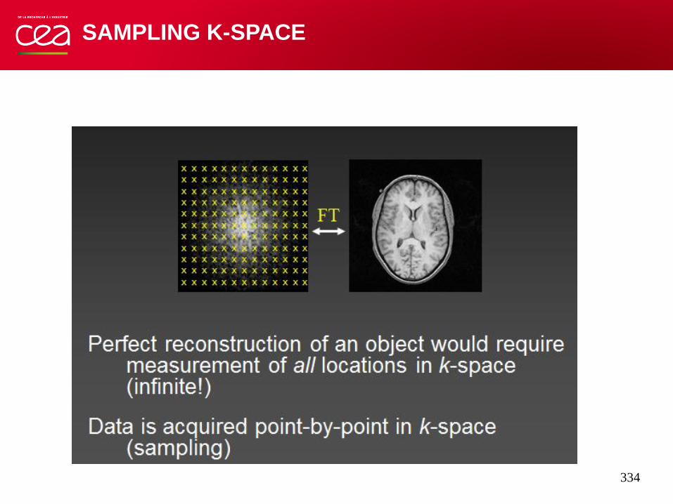
SAMPLING K-SPACE
334

13
SAMPLING K-SPACE
335

What is the maximum
frequency we need to measure?
Or, what is the maximum k-
space value we must sample
(kmax)?
FT
kmax -kmax
FREQUENCY SPECTRUM
335-a

FREQUENCY SPECTRUM
335-b

FREQUENCY SPECTRUM
335-c

FREQUENCY SPECTRUM
335-d

FREQUENCY SPECTRUM
335-e

FREQUENCY SPECTRUM
335-f

Higher frequencies make the
reconstruction look more like the original
object!
Large kmax increases resolution (allows us to
distinguish smaller features)
FREQUENCY SPECTRUM
335-g

21
CHOOSING MAXIMAL FREQUENCY
336

22
NYQUIST SAMPLING THEOREM
337

23
NYQUIST SAMPLING THEOREM
338

24
ALIASING ARTIFACT
339
25
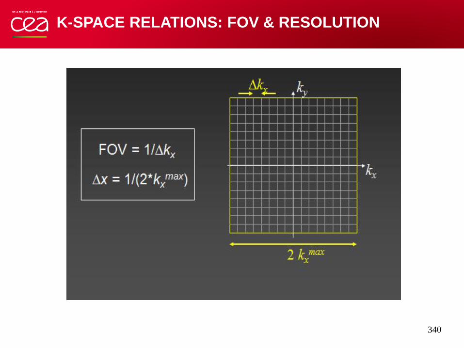
K-SPACE RELATIONS: FOV & RESOLUTION
340
26
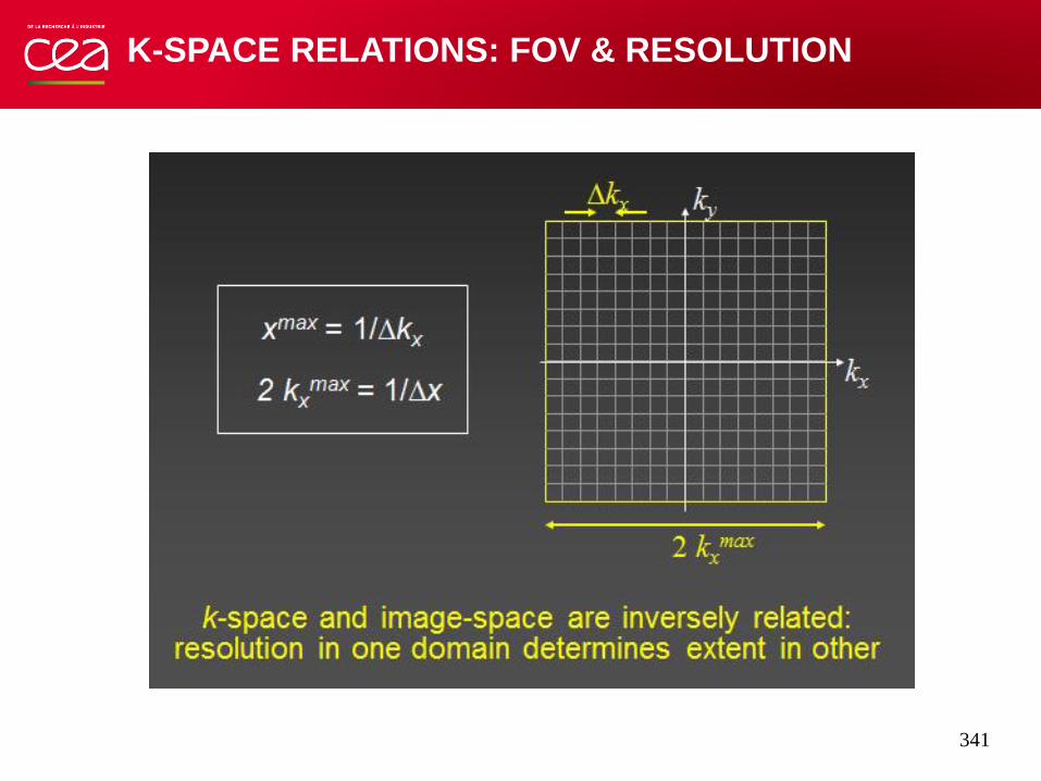
K-SPACE RELATIONS: FOV & RESOLUTION
341

STANDARD MR IMAGE RECONSTRUCTION
342

PARTIAL FOURIER
343

OUTLINE
Part I: Background in Magnetic Resonance Imaging • MRI scanner
• Sampling k-space & Cartesian reconstruction
• Trajectories and acquisition strategies
• Image reconstruction strategies
344

K-SPACE TRAJECTORY MODELING
K-space location is proportional to accumulated area under
gradient waveforms 345

K-SPACE TRAJECTORY CONSTRAINTS
346

EXAMPLES: RASTER-SCAN 2D DFT ACQUISITION
347

EXAMPLES: ECHO PLANAR IMAGING (EPI)
ACQUISITION
348

IMAGE QUALITY VS. ACQUISITION TIME
349

IMAGE QUALITY VS. ACQUISITION TIME
350
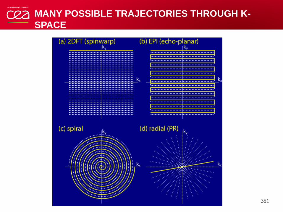
MANY POSSIBLE TRAJECTORIES THROUGH K-
SPACE
351

NON-CARTESIAN MR IMAGE RECONSTRUCTION
3502
OUTLINE
Part I: Background in Magnetic Resonance Imaging • MRI scanner
• Sampling k-space & Cartesian reconstruction
• Trajectories and acquisition strategies
• Image reconstruction strategies
353

TEXTBOOK MRI MEASUREMENT MODEL
354
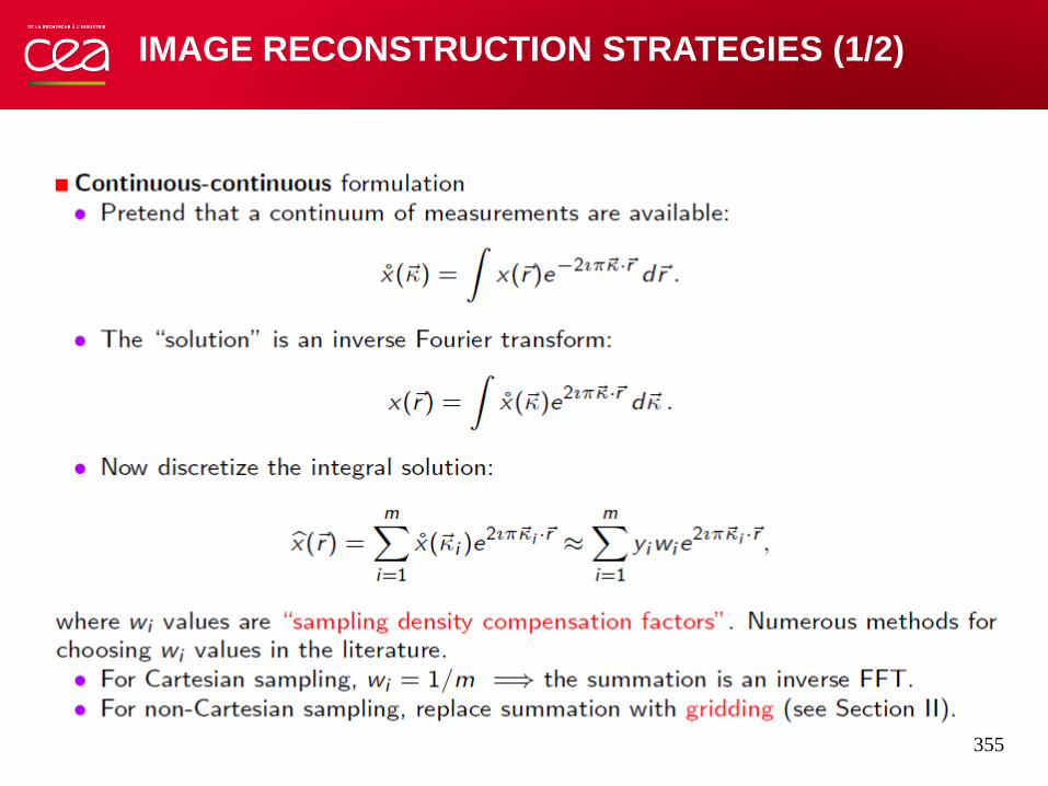
IMAGE RECONSTRUCTION STRATEGIES (1/2)
355
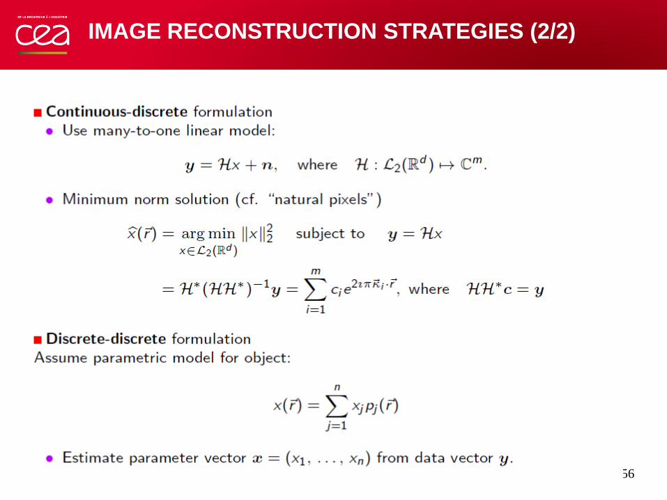
IMAGE RECONSTRUCTION STRATEGIES (2/2)
356

OUTLINE
Part II:Non-Cartesian MRI reconstruction
Prof. John Pauly

NON-CARTESIAN MRI
• K-space trajectory does not fall on a Cartesian grid: Spiral, radial, Lissajou
• Faster, more robust to motion than Cartesian MRI
• But reconstruction is more complicated …
Spiral Lissajou
358

RECONSTRUCTION OF NON-CARTESIAN MRI
DATA
• Direct FFT won’t work
• Radial MRI: backprojection reconstruction, like in CT
• In general:
- Compute the inverse DFT according to the trajectory (slow). Cf Conjugate Phase reconstruction.
- Regridding: resample the non-Cartesian MRI data onto a 2D Cartesian grid and apply inverse FFT (fast)
359
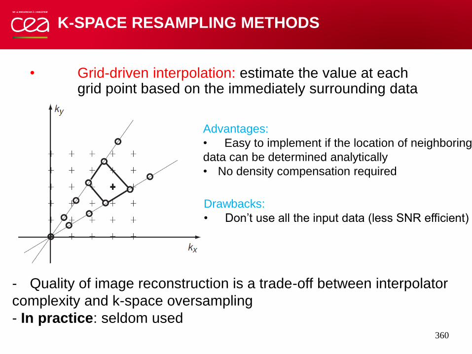
K-SPACE RESAMPLING METHODS
• Grid-driven interpolation: estimate the value at each grid point based on the immediately surrounding data
Advantages:
• Easy to implement if the location of neighboring
data can be determined analytically
• No density compensation required
Drawbacks:
• Don’t use all the input data (less SNR efficient)
- Quality of image reconstruction is a trade-off between interpolator
complexity and k-space oversampling
- In practice: seldom used 360

K-SPACE RESAMPLING METHODS
• Data-driven interpolation: take each data point and add its contribution to the surrounding grid points
Advantage:
• All data points are used: more SNR efficient
Drawback:
• Require density estimation & compensation
- Convolve with a k-space kernel.
- Evaluate the convolution at the adjacent grid
points.
361

MATHEMATICAL DESCRIPTION OF GRIDDING
RECONSTRUCTION
362

EFFECTS OF REGRIDDING OPERATIONS
Original signal
Blurring + side lobes
1D Illustration
Apodization
Replication
363

SIMPLE REGRIDDING
• 5 point triangular kernel
364
Without density compensation, low frequency artifacts dominate

REGRIDDING DESIGN CONSIDERATIONS
• Non-Cartesian sampling trajectory
Sampling pattern (PSF) & sidelobes
Density compensation
• Convolution kernel
Apodization
Aliasing
Computation time
• Oversampling
Aliasing
Apodization
365

VARIABLE DENSITY SAMPLING (1/2)
• Non-Cartesian trajectories perform a variable-density sampling
of k-space
Variable Density Spiral Radial
Radial: The central point is acquired N times (# the number of spokes)
Non-uniform k-space weighting
366
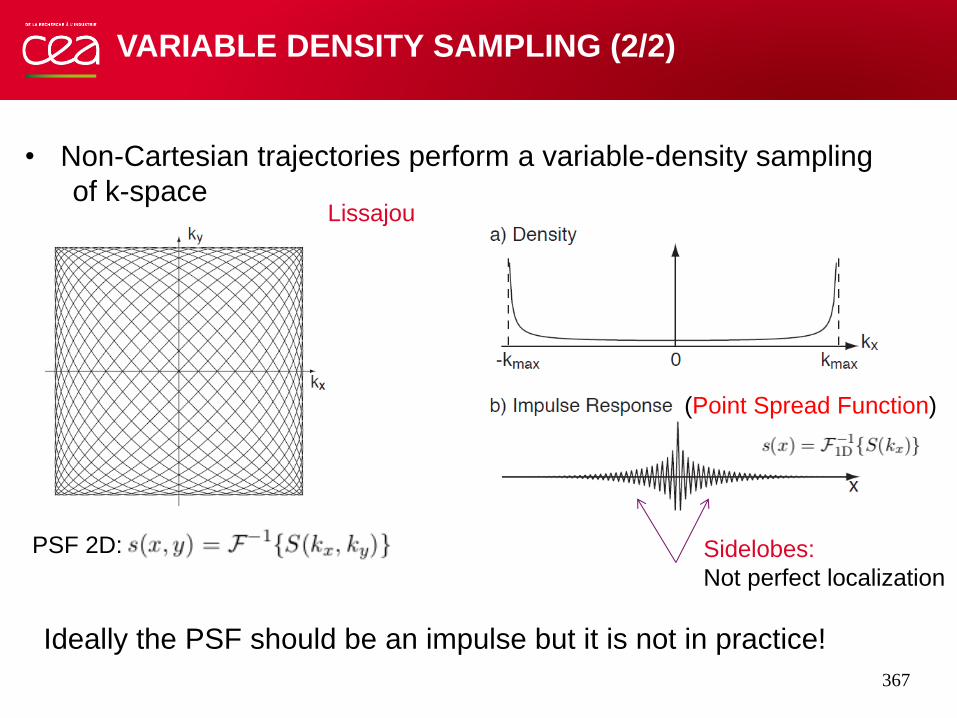
VARIABLE DENSITY SAMPLING (2/2)
• Non-Cartesian trajectories perform a variable-density sampling
of k-space
Lissajou
Sidelobes:
Not perfect localization
Ideally the PSF should be an impulse but it is not in practice!
(Point Spread Function)
PSF 2D:
367

SAMPLING DENSITY COMPENSATION (1/4)
• Pre-compensation (ideal)
368

SAMPLING DENSITY COMPENSATION: VORONOI
DIAGRAM (2/4)
Nine-interleave k-space spiral Voronoi diagram
Density approximated as the inverse of the area of these regions
Region for a
given sample
369
[Rasche et al, IEEE TMI 1999]

SAMPLING DENSITY COMPENSATION (3/4)
• Post-compensation (after the gridding operation)
• It works well if the sampling pattern does not change too rapidly
• The gridding convolution kernel blurs the effect of rapid density
changes
370

EFFECT OF DENSITY COMPENSATION ON MR
IMAGE RECONSTRUCTION (4/4)
371
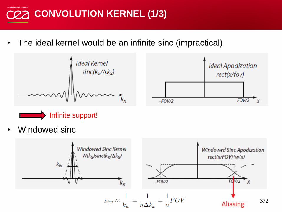
CONVOLUTION KERNEL (1/3)
• The ideal kernel would be an infinite sinc (impractical)
• Windowed sinc
Infinite support!
372
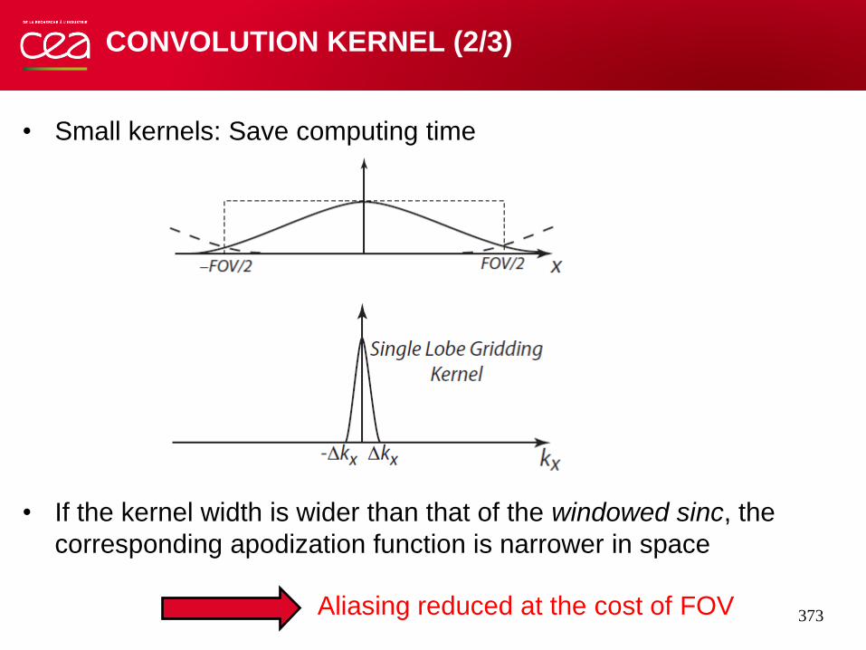
CONVOLUTION KERNEL (2/3)
• Small kernels: Save computing time
• If the kernel width is wider than that of the windowed sinc, the
corresponding apodization function is narrower in space
Aliasing reduced at the cost of FOV 373

CONVOLUTION KERNEL (3/3)
• Kaiser-Bessel function: smooth lowpass filter
Best kernel (by consensus)
374
[Jackson et al, IEEE TMI 1991]
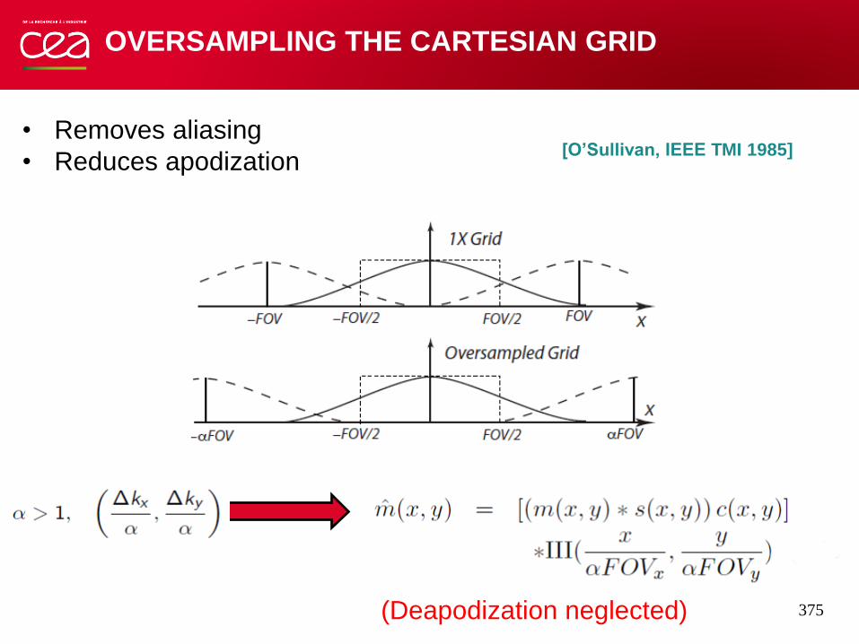
OVERSAMPLING THE CARTESIAN GRID
• Removes aliasing
• Reduces apodization
(Deapodization neglected) 375
[O’Sullivan, IEEE TMI 1985]

OVERSAMPLING THE CARTESIAN GRID
376
Radial
Spiral
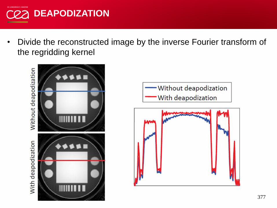
DEAPODIZATION
• Divide the reconstructed image by the inverse Fourier transform of
the regridding kernel
377

WHY THE KAISER-BESSEL KERNEL IS
PREFERRED?
• Lower oversampling factor (save memory)
FFTW package:
fftw.org
Fast implementations
of FFT for a whole
range of lengths
378
[Beatty et al, IEEE TMI 2005]

SUMMARY OF REGRIDDING RECONSTRUCTION
• Compute the non-Cartesian sampling pattern
• Choose the regridding kernel (e.g. Kaiser-Bessel)
• Density pre-compensation (if possible)
• Convolve the pre-compensated data with the regridding kernel and
evaluate the convolution at the oversampled Cartesian grid
• Apply inverse 2D FFT
• Apply the deapodization function
• Apply post-density post-compensation (optional)
• Remove the oversampling by cropping the image 379
OUTLINE
Part III: Iterative Model-based image reconstruction • Least squares solution
• Regularized Least Squares
• Beyond quadratic regularization
Prof. Jeff Fessler
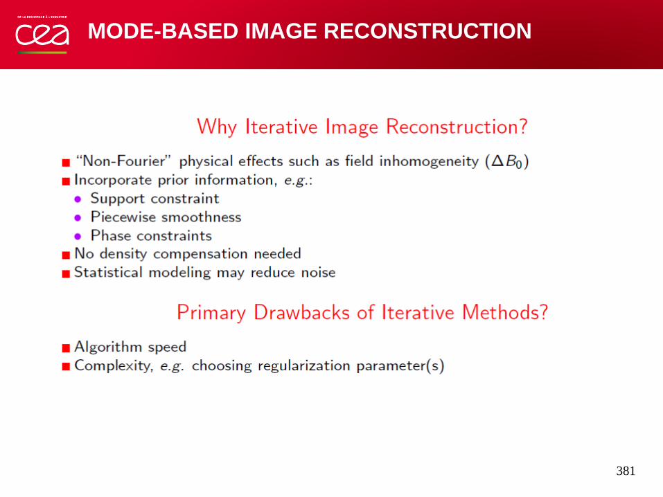
MODE-BASED IMAGE RECONSTRUCTION
381

BASIC SIGNAL MODEL
382

LEAST SQUARES ESTIMATION
383
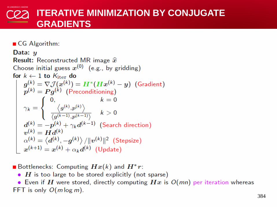
ITERATIVE MINIMIZATION BY CONJUGATE
GRADIENTS
384
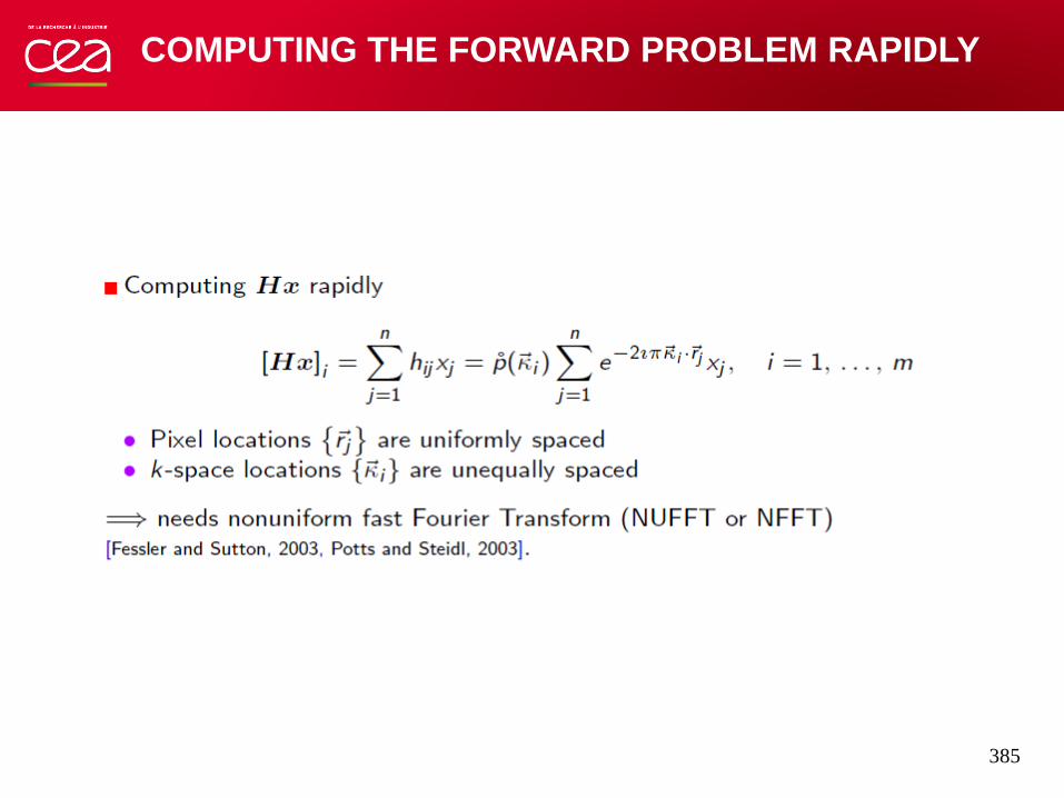
COMPUTING THE FORWARD PROBLEM RAPIDLY
385

NUFFT (TYPE 2)
385

FURTHER ACCELERATION USING TOEPLITZ
MATRICES
387

UNREGULARIZED EXAMPLE: SIMULATED DATA
• 4x undersampled radial k-space data
• Analytical k-space generation 388

UNREGULARIZED EXAMPLE: IMAGES
• Iterations: 1:4:60 of unregularized CG reconstruction 389

UNREGULARIZED EXAMPLE: RMS ERROR
• Complexity: When to stop A solution: regularization 390

UNREGULARIZED EIGENSPECTRUM
• Bad conditioning i.e. extremely large condition number ⋍ 1020 391

REGULARIZED EXAMPLE: IMAGE COMPARISON
392

REGULARIZED EXAMPLE: RMS ERROR
393

REGULARIZED LEAST SQUARES ESTIMATION
394

QUADRATIC REGULARIZATION
395

CHOOSING THE REGULARIZATION PARAMETER
396

SPATIAL RESOLUTION EXAMPLE
𝑻𝒆𝒋 𝜶𝑪𝒕𝑪𝒆𝒋 PSF
𝑻(𝝎) 𝑹(𝝎) L(𝝎)
Radial k-space trajectory, FWHM of PSF is 1.2 pixels 397

SPATIAL RESOLUTION EXAMPLE: PROFILES
𝑻(𝝎)
𝑹(𝝎)
L(𝝎)
398

RESOLUTION/NOISE TRADE-OFFS
399

RESOLUTION/NOISE TRADE-OFFS EXAMPLE
In short: one can choose 𝛼 rapidly and predictably for quadratic regularization 400

NON-QUADRATIC REGULARIZATION
401
[Charbonnier et al, IEEE IP 997]

NON-QUADRATIC POTENTIAL FUNCTIONS
Lower cost for large differences edge preservation 402

EDGE-PRESERVING REGULARIZATION EXAMPLE
403
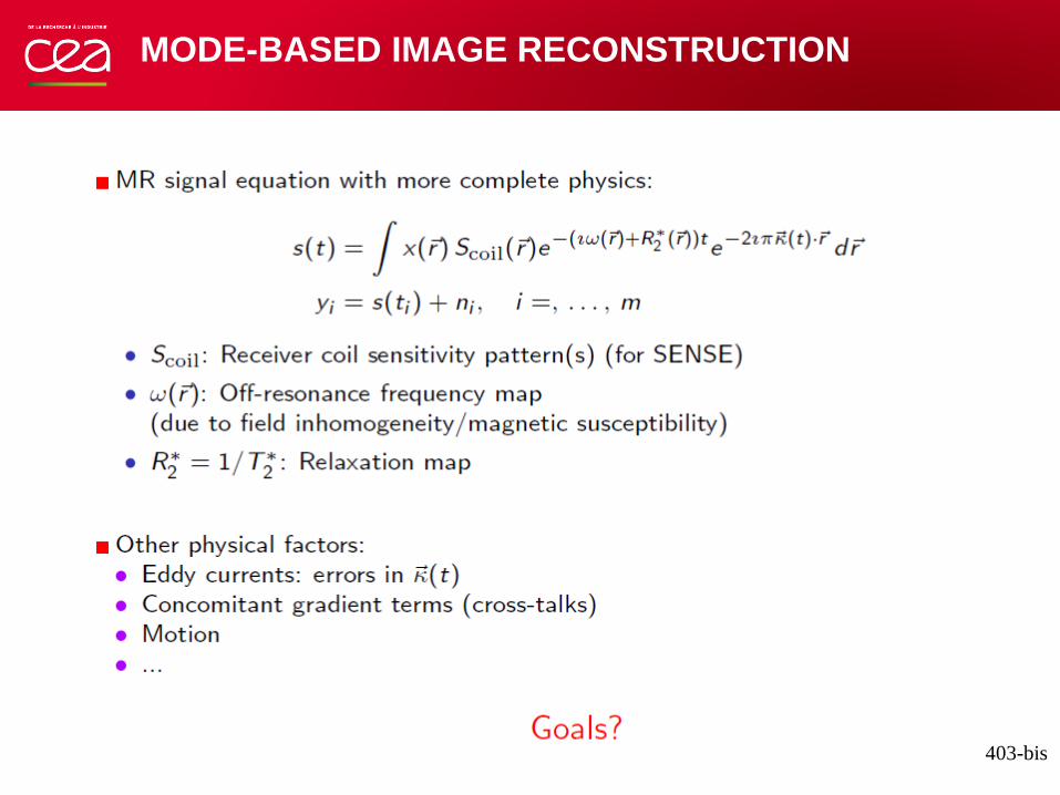
MODE-BASED IMAGE RECONSTRUCTION
403-bis

FIELD INHOMOGENEITY –CORRECTED
RECONSTRUCTION
403-ter
OUTLINE
Part IV: Parallel imaging
404

BACKGROUND: MRI IS SLOW…
Michael Lustig, http://www.eecs.berkeley.edu/~mlustig/CS.html
405
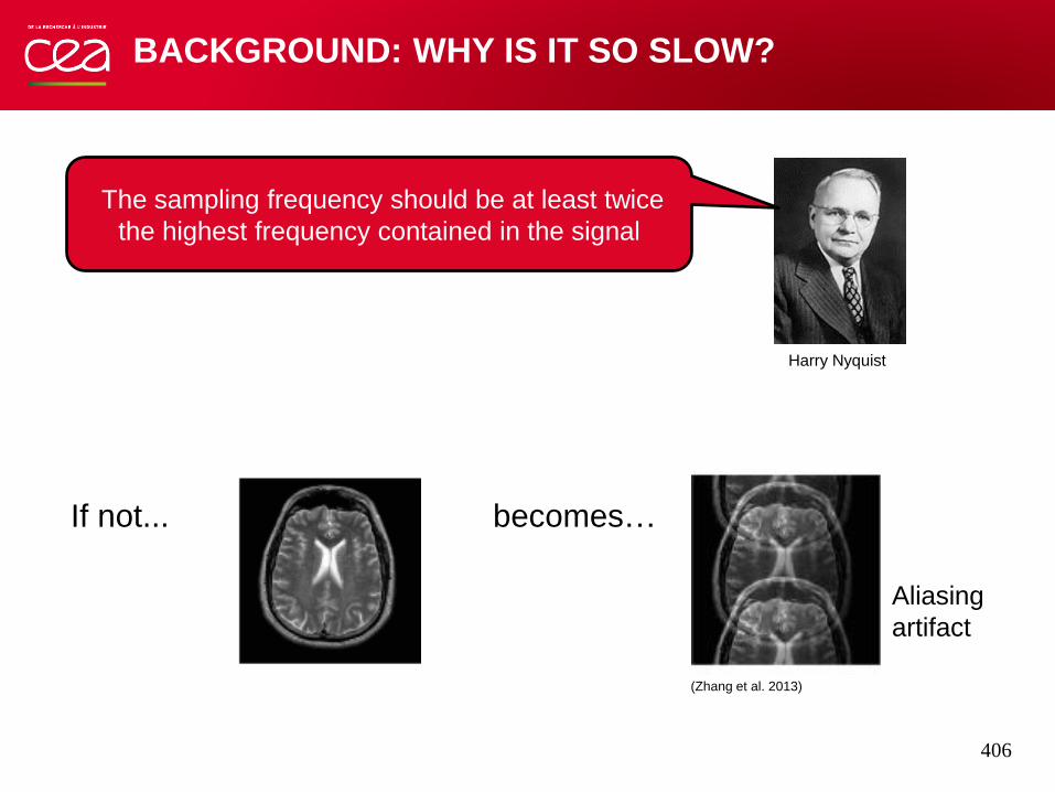
BACKGROUND: WHY IS IT SO SLOW?
If not... becomes…
Harry Nyquist
The sampling frequency should be at least twice
the highest frequency contained in the signal
Aliasing
artifact
(Zhang et al. 2013)
406

EXAMPLE: 3D-image of Baboon whole Brain T2*
at high resolution iso-200m
Nova Medical 1Tx/32Rx
Natif SNR7.6 (WM)
FOV 205x205x52mm3
Matrix: 1024x1024x256
~270 million samples!!
1 average only!
Displayed Reco:
0.2x0.2x0.2mm3
TA2h54min
Raw data size: 137GB
Dicom data size: 1.0GB
(Courtesy of A. Vignaud & S.
Mériaux)
Not applicable
for humans!
407

UNDERSAMPLING TO REDUCE ACQUISITION TIME
UNDERSAMPLING
Multiple receiver coils
SMS Parallel Imaging
Single receiver coil
Partial Fourier Compressed
Sensing
Limitations: - R = acceleration factor ≤ 6
- SNR drops rapidly with R
Possible
combination
Can we reduce the acquisition time by measuring fewer samples and still be
able to reconstruct nice images?
408

Combining the signal of multiple coils
✓ Reduce scan
time
✓ Improve spatial
/ temporal
resolution
✓ Limit geometric
distorsions
✘ Decrease the
SNR
✘ Non-
homogeneous
coils
OBJECTIVES OF PARALLEL IMAGING (PMRI)
409

EXAMPLE IN ANATOMICAL MRI
Reduce scanning time at fixed spatial resolution
Standard acquisition Parallel acquisition Parallel acquisition
410

EXAMPLE IN FUNCTIONAL MRI (EPI SEQUENCE)
Improve spatial resolution at fixed TR
Standard acquisition Parallel acquisition Parallel acquisition
411

PARALLEL MRI PRINCIPLE
Phase e
ncodin
g
Frequency encoding
Standard acquisition parallel acquisition using R=2
412

SPATIAL COIL SENSITIVITIES
413

101
PARALLEL MRI RECONSTRUCTION TECHNIQUES
414

Full k-space sampling
k-space Under-sampling
(R=2)
Acceleration factor
K-SPACE ACQUISITION
Aliasing artifacts
415

K-SPACE ACQUISITION
Full k-space sampling
k-space Under-sampling
(R=2)
Acceleration factor y 𝑟 = 𝑥 𝑟1 + 𝑥 𝑟2
𝑥(𝑟1)
𝑥(𝑟2)
416

[Pruessman et al, MRM 1999] 2 coils R=2
SENSITIVITY ENCODING IMAGING
𝑦1 𝑟 = 𝑆1 𝑟 1 𝑥 𝑟 1 + 𝑆1 𝑟 2 𝑥 𝑟 2 + 𝑛1 𝑟 𝑦 𝑟 = 𝑆2 𝑟 1 𝑥 𝑟 1 + 𝑆2 𝑟 2 𝑥 𝑟 2 + 𝑛2 𝑟
𝑦1 𝑟
𝑦2 𝑟 =
𝑆1 𝑟 1 𝑆1 𝑟 2𝑆2 𝑟 1 𝑆2 𝑟 2
𝑥 𝑟 1𝑥 𝑟 2
+ 𝑛1 𝑟
𝑛2 𝑟
𝑟 1 = 𝑟
𝑟 2 = 𝑟 +𝐹𝑂𝑉𝑦
2
417

[Pruessman et al, MRM 1999] L coils R acceleration factor
𝑦𝐿 𝑟 = 𝑆𝐿 𝑟 1 𝑥 𝑟 1 + 𝑆𝐿 𝑟 2 𝑥 𝑟 2 + … + 𝑆𝐿 𝑟 𝑅 𝑥 𝑟 𝑅 + 𝑛𝐿 𝑟
L
𝑦1 𝑟
𝑦2 𝑟 ⋮
𝑦𝐿 𝑟
=
𝑆1 𝑟 1 … 𝑆1 𝑟 𝑅𝑆2 𝑟 1 … 𝑆2 𝑟 𝑅⋮
𝑆𝐿 𝑟 1
⋱…
⋮𝑆𝐿 𝑟 𝑅
𝑥 𝑟 1𝑥 𝑟 2⋮
𝑥 𝑟 𝑅
+
𝑛1 𝑟
𝑛2 𝑟 ⋮
𝑛𝐿 𝑟
y(𝒓) = 𝑺(𝒓) 𝒙(𝒓) + 𝒏(𝒓) Simultaneous reconstruction of R pixels of the full FOV image
SENSITIVITY ENCODING IMAGING
𝑟 𝑗 = 𝑟 + 𝑗𝐹𝑂𝑉𝑦
𝑅
418

SENSE Reconstruction (R=4)
COMPLEX-VALUED DATA
𝒚𝑪(𝒓) = 𝑺𝑪 (𝒓) 𝒙𝑪 (𝒓) + 𝒏𝑪(𝒓)
𝑦𝑅 𝑟
𝑦𝐼 𝑟 =
𝑆𝑅 𝑟 −𝑆𝐼 𝑟
𝑆𝐼 𝑟 𝑆𝐼 𝑟 𝑥𝑅 𝑟
𝑥𝐼 𝑟 +
𝑛𝑅 𝑟
𝑛𝐼 𝑟
419

Reference Image SENSE Reconstruction (R=4)
SENSE RECONSTRUCTION
420

RESULTS AT 1.5 TESLA
• Artifacts appear for large values of R
421
𝛒ˆ= 𝐒𝐇𝐒 + λ𝚫
−1𝐒𝐇𝐝
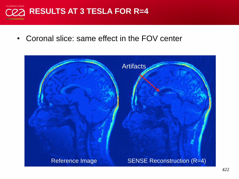
Reference Image SENSE Reconstruction (R=4)
RESULTS AT 3 TESLA FOR R=4
Artifacts
• Coronal slice: same effect in the FOV center
422

REGULARIZED SENSE RECONSTRUCTION
423

REGULARIZED SENSE RECONSTRUCTION
424

MR images: sparse in the wavelet domain
Daubechies’
2D-wavelet
Haar’s
1D-wavelet
Spatial domain Wavelet domain
● Improved spatial and frequency artifact localization ● Simple and accurate statistical model in the wavelet space
Image histogram Wavelet subband histogram
Gauss-Laplace pdf
WAVELETS ENTER INTO THE GAME …
𝚽∗
𝚽
425
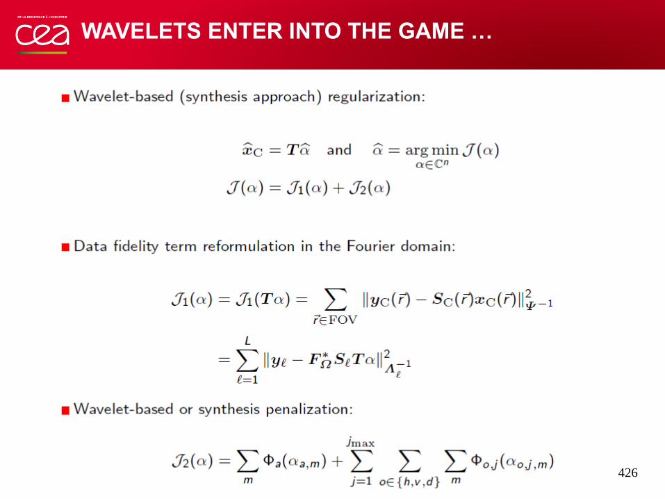
WAVELETS ENTER INTO THE GAME …
426

PROXIMAL OPERATORS (1/3)
427

PROX. OPERATOR: GENERALIZED PROJECTION
(2/3)
428

PROX. OPERATOR: SEPARABLE SUM (3/3)
429

PROXIMAL GRADIENT ALGORITHM
430

FORWARD BACKWARD OPTIMIZATION
430-bis

WAVELET-BASED RESULTS
[Chaari et al, IEEE ISBI 2008]
431

CONSTRAINED REGULARIZATION
[Chaari et al, MedIA 2011]
432

CONSTRAINED CONVEX OPTIMIZATION
[Chaari et al, MedIA 2011]
433

CONSTRAINED WAVELET-BASED RESULTS
[Chaari et al, MedIA 2011]
434

ANALYSIS & SYNTHESIS REGULARIZED RESULTS
[Chaari et al, MedIA 2011]
435

ZOOMING
[Chaari et al, MedIA 2011]
436

[Chaari et al, IEEE ISBI 2011]
3D REGULARIZATION & RECONSTRUCTION
437
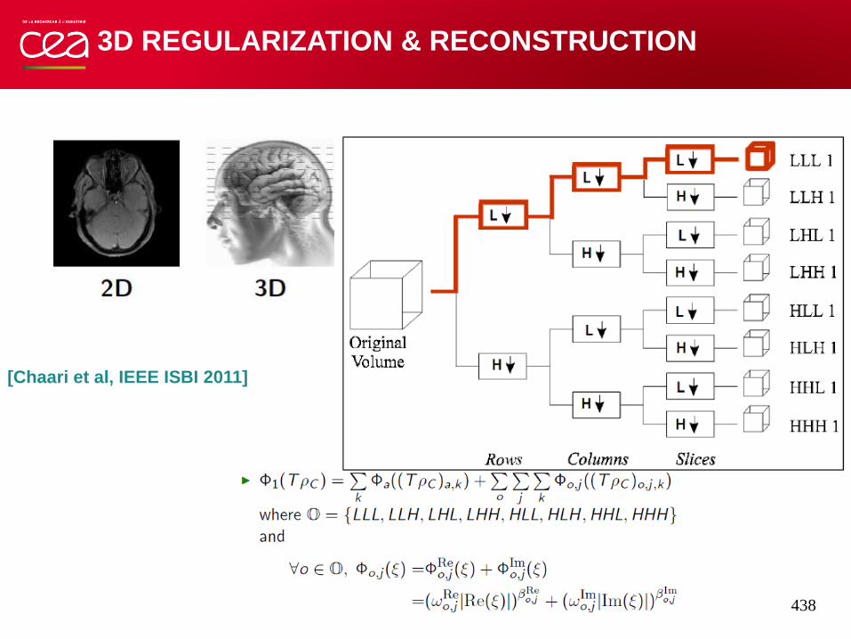
3D REGULARIZATION & RECONSTRUCTION
[Chaari et al, IEEE ISBI 2011]
438

3D UWR-SENSE SEGMENTATION RESULTS
[Chaari et al, MAGMA 2014] 439

OUTLINE
Part V: Compressed Sensing in MRI
440

COMPRESSED SENSING CONCERN: WHEN IMAGE
ACQUISITION MEETS IMAGE RECONSTRUCTION
441

COMPRESSED SENSING CONCERN: WHEN IMAGE
ACQUISITION MEETS IMAGE RECONSTRUCTION
442

COMPRESSED SENSING IN MRI
iFFT
K-space
443

COMPRESSED SENSING IN IRM
??
?? ??
K-space
• What images?
• What samples?
• What reconstruction technique?
[Lustig et al, MRM 2007]
444

COMPRESSED SENSING RECIPE
Data is sparse, compressible, redundant…
Sense the compressed information directly!
Donoho, Tao,
Romberg, Candes
Michael Lustig, http://www.eecs.berkeley.edu/~mlustig/CS.html
445

WHAT SPARSITY AND COMPRESSIBILITY MEAN?
1. Sparsity/Compressibility
Sparse
(spärs),
adj. spars•er, spars•est.
1. Thinly scattered or distributed; not thick
or dense.
2. Scanty; meager. (http://www.thefreedictionary.com/sparse)
Compressible
1. There exists a basis where the
representation has just a few large
coefficients and many small coefficients.
2. Compressible signals are well
approximated by sparse representations
(www.healthcare.siemens)
Angiography image… is sparse is not sparse…
… but compressible!
3 levels of
decomposition
Wavelet Represensation… is sparse!
446

Curvelets
Starlets, shearlets
Redundant transforms
𝜱 induces sparser
decompositions 𝜶
COMPRESSED SENSING RECIPE (1/3)
• Increase sparsity by changing the image decomposition
447
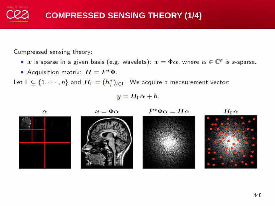
COMPRESSED SENSING THEORY (1/4)
448

COMPRESSED SENSING THEORY (2/4)
449

COMPRESSED SENSING THEORY (3/4)
(FISTA algorithm) 450

COMPRESSED SENSING THEORY (4/4)
(ADMM algorithm) 451
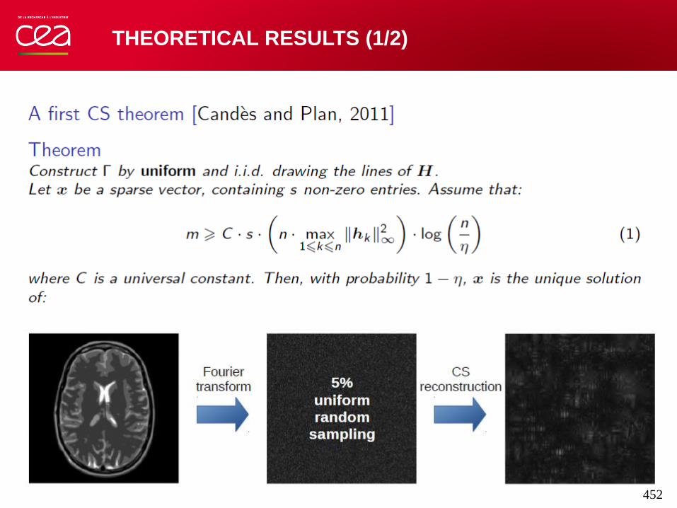
THEORETICAL RESULTS (1/2)
452

DFT
DFT
No
n-u
nifo
rm s
am
plin
g
2. Pseudo-random sampling
• Non-uniform sampling
FROM UNIFORM RANDOM UNDERSAMPLING TO VDS
• Variable Density Sampling
COHERENT FOLDING
INCOHERENT ARTIFACT
Un
ifo
rm s
am
plin
g
Noise-like
(Lustig et al. 2007, Chauffert et al. 2013, Puy et al. 2011)
Lustig et al. 2008 453
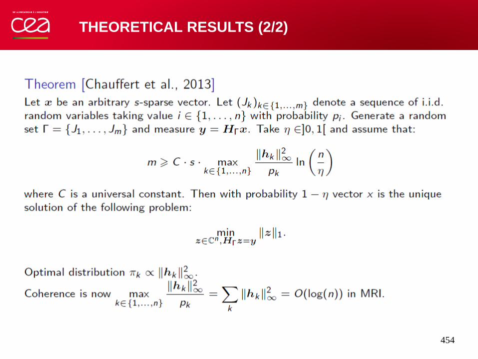
THEORETICAL RESULTS (2/2)
454
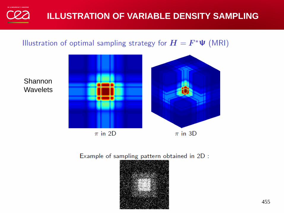
ILLUSTRATION OF VARIABLE DENSITY SAMPLING
Shannon
Wavelets
455
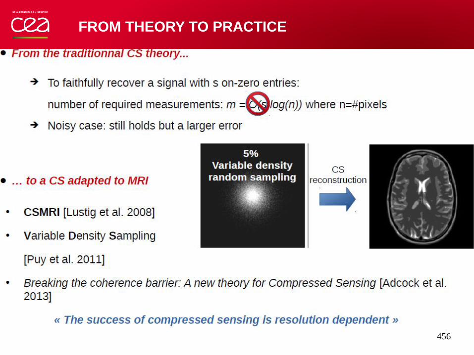
FROM THEORY TO PRACTICE
456

CS-MRI AND EXISTING RESULTS
• CS must comply with MR hardware constraints
𝜅 𝑡 = 𝜅 0 + 𝛾 𝐺 𝑢 𝑑𝑢𝑡
0
Regular trajectories
• Easy implementation: undersampling standard MR trajectories!
• Radial for cardiac cine MR imaging (Winkelmann et al. 2007)
• Spiral or noisy spirals (Lustig et al. 2005)
• Poisson disk sampling (Vasanawala et al. 2011)
𝐺 < 𝐺𝑚𝑎𝑥 ≈ 50 𝑚𝑇𝑚−1
𝐺 < 𝐺 𝑚𝑎𝑥 ≈ 333 𝑇𝑚−1𝑠−1
Lustig et al. 2008
7T MRI
457

CS-MRI AND EXISTING RESULTS
Lustig et al. 2007
CS is not used to its full potential!
• Hindered randomness
• Variable density sampling not fulfilled
• K-space not well covered or oversampled in one direction
Undersampling factor generally limited to : R ≤ 10
458
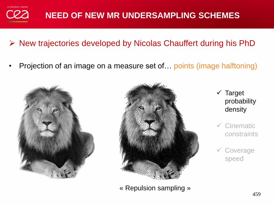
NEED OF NEW MR UNDERSAMPLING SCHEMES
New trajectories developed by Nicolas Chauffert during his PhD
• Projection of an image on a measure set of… points (image halftoning)
Target
probability
density
Cinematic
constraints
Coverage
speed
« Repulsion sampling » 459

NEED OF NEW MR UNDERSAMPLING SCHEMES
New image approximation techniques [Chauffert et al, Construct. Approx., 2016]
• Projection of an image on a measure set of… curves (image stippling)
Target
probability
density
Cinematic
constraints
Coverage
speed
460

NEED OF NEW MR UNDERSAMPLING SCHEMES
Application to design of k-space trajectories
Target
probability
density
Gradient
constraints
Coverage
speed
Variable Density
𝐺 < 𝐺𝑚𝑎𝑥 ≈ 50 𝑚𝑇𝑚−1
𝐺 < 𝐺 𝑚𝑎𝑥 ≈ 333 𝑇𝑚−1𝑠−1
[Chauffert et al, IEEE TMI 2016; Chauffert et al, SIAM Imaging Sci 2016]
461
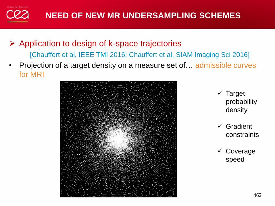
NEED OF NEW MR UNDERSAMPLING SCHEMES
Application to design of k-space trajectories
• Projection of a target density on a measure set of… admissible curves
for MRI
Target
probability
density
Gradient
constraints
Coverage
speed
[Chauffert et al, IEEE TMI 2016; Chauffert et al, SIAM Imaging Sci 2016]
462

VERY HIGH RESOLUTION IMAGING: SIMULATION
SETUP
463

VERY HIGH RESOLUTION IMAGING: SIMULATION
SETUP
464

| PAGE 156 UNIRS | 03-02-2016
VERY HIGH RESOLUTION IMAGING: COMPETING
TRAJECTORIES (1/2)
465

| PAGE 157 UNIRS | 03-02-2016
VERY HIGH RESOLUTION IMAGING: COMPETING
TRAJECTORIES (2/2)
466

VERY HIGH RESOLUTION IMAGING CS RESULTS (1/2)
467

VERY HIGH RESOLUTION IMAGING CS RESULTS (2/2)
468
CS SUMMARY
469