Eur. Phys. J. B 23, 153–158 (2001) THE EUROPEANPHYSICAL JOURNAL Bc©

EDP SciencesSocieta Italiana di FisicaSpringer-Verlag 2001

Magnetic properties of undoped YBa2Cu3O6+x system

Govind1,a, A. Pratap1, Ajay2, and R.S. Tripathi2

1 Theory Group, National Physical Laboratory, Dr. K.S. Krishnan Marg, New Delhi 110012, India2 Department of Physics, G.B. Pant University of Ag. & Tech. Pantnagar 263145, India

Received 13 July 2000 and Received in final form 14 May 2001

Abstract. In the present paper, we study the magnetic properties of bilayer cuprate antiferromagnets.In order to evaluate the expressions for spin-wave dispersion, sublattice magnetization, Neel temperatureand the magnetic contribution to the specific heat, the double time Green’s function technique has beenemployed in the random phase approximation (RPA). The spin wave dispersion curve for a bilayer anti-ferromagnetic system is found to consist of one acoustic and one optic branch. The “optical magnon gap”has been attributed solely to the intra-bilayer exchange coupling (J⊥) as its magnitude does not changesignificantly with the inter-bilayer exchange coupling (Jz). However Jz is essential to obtain the acousticmode contribution to the magnetization. The numerical calculations show that the Neel temperature (TN)of the bilayer antiferromagnetic system increases with the Jz and a small change in Jz gives rise to alarge change in the Neel temperature of the system. The magnetic specific heat of the system follows a T 2

behaviour but in the presence of Jz it varies faster than T 2.

PACS. 75.30.-m Intrinsic properties of magnetically ordered materials – 74.72.Bk Y-based cuprates –75.10.Jm Quantized spin models

1 Introduction

In the undoped state, the cuprate superconductors likeLa2CuO4, and YBa2Cu3O6 (123) are layered antiferro-magnetic (AFM) insulators. Due to their layered structurethese systems possess anisotropy in many of their physi-cal properties. The La2CuO4 system has only one CuO2

plane per unit cell. The magnetic properties in the in-sulating phase of this material can be well described bythe Heisenberg model with in-plane AFM exchange cou-pling (J‖) and inter unit cell exchange coupling (Jz) [1–8].On the other hand, YBa2Cu3O6 has two layers per unitcell and the electronic states of these CuO2 layers arestrongly coupled right from the undoped to overdopedphase [9–13]. Therefore unlike single layered La2CuO4 sys-tem the study of magnetic dynamics of bilayer system re-quires extra attention.

It has been observed in YBa2Cu3O6+x, that the intra-bilayer coupling (J⊥) leads towards the presence of anacoustic and an optic mode in the magnon dispersion anda magnon gap of the order of 65–70 meV [14]. It hasalso been observed [15] that inter-bilayer exchange cou-pling (Jz) is important to establish long range order (3DNeel ordering) in these systems and plays a significant rolein the magnetic dynamics.

Several theoretical efforts have been made to inves-tigate the normal state magnetic properties of cupratesystems. These calculations mainly deal with the single

a e-mail: govind@csnpl.ren.nic.in

layer and two-sublattice models within the random phaseapproximation [1,2], spin-waves [3], the Callen decou-pling scheme [4] and the Schwinger boson approach [6,7].By contrast, to date, theoretical studies for the bilayercuprates have been performed by considering the in-plane and the intra-bilayer exchange coupling only. Milliset al. [16,17] have calculated the dynamical susceptibilityof these systems within the Schwinger boson technique.They estimated that the intra-bilayer exchange couplingstrength (J⊥) is about 14 meV. Du et al. [18] have shownthat in the absence of intra- or inter- bilayer exchangecoupling the system does not show long range magneticorder and the Neel temperature vanishes.

More recently, we have discussed the magnetic dynam-ics of a bilayer antiferromagnetic system (YBa2Cu3O6+x)within linear spin wave approximation [15]. In this study,we consider in-plane and intra-bilayer exchange couplingin the model Hamiltonian while the role of inter-bilayer ex-change coupling was introduced phenomenologically. Wehave examined the role of the optic and acoustic magneticexcitations on the magnetic dynamics of bilayer systemsand found that in the absence of anisotropy, the acousticmode may not sustain magnetization.

In view of this, in the present paper, we incorporate theeffects of inter-bilayer exchange coupling explicitly intothe microscopic model Hamiltonian and plan to study itsrole on the magnetic properties of bilayer cuprates. Weemploy Green’s function formalism [19] for a four sublat-tice model within the random phase approximation and

154 The European Physical Journal B

H = J‖X

i6=j,α6=β[SiaαSjbα + SjaαSibα + SicαSjdα + SjcαSidα]

+ J⊥Xi,α6=β

[SiaαSicβ + SiaβSicα + SibαSidβ + SibβSidα]

+ JzXi,α6=βδ′

[SiaαSi+δ′cβ + SiaβSi+δ′cα + SibαSi+δ′dβ + SibβSi+δ′dα] ,

obtain expressions for sublattice magnetization, Neel tem-perature and magnetic specific heat for bilayer antiferro-magnets. We organize the paper in the following way. Thetheoretical formulation is presented in Section 2. Expres-sions for staggered magnetization, Neel temperature andmagnetic specific heat are presented in Sections 3, 4, 5 re-spectively. The numerical results and discussions are givenin Section 6.

2 Theoretical formulation

For bilayer systems, we define the Heisenberg antiferro-magnetic Hamiltonian as:

H = J⊥∑i,j,α

SiαSjα + J⊥∑i,α

SiαSiβ + Jz∑i,δ′

SiαSi+δ′β .

(1)

In four sublattice model the above Hamiltonian can beexplicitly written as

see equation above

where, αβ = 1(2) are the layer indices, i, j denotes thelattice sites with j is the nearest neighbour of i, δ is thenearest neighbour distance within plane and δ′ is the dis-tance between the two bilayers. The suffixes a, b, c and ddenote the four sublattices of the system. J‖ is the in-planeexchange coupling and J⊥, Jz are intra- and inter-bilayerexchange couplings respectively. A figure describing vari-ous exchange couplings for a bilayer system with four basisatoms (a, b, c, and d) is shown in Figure 1. We define forthis purpose the following Green’s functions

G1 = 〈〈S+ia1;S−ia1〉〉 G2 = 〈〈S+

ib1;S−ia1〉〉G3 = 〈〈S+

ic2;S−ia1〉〉 G4 = 〈〈S+id2;S−ia1〉〉 (2)

where S± = Sx ± iSy are the spin raising and loweringoperators. The equation of motion for the Green’s function〈〈S+

ia1;S−ia1〉〉 can be written as

ωG1 =1

2π⟨ [S+ia1;S−ia1

] ⟩+⟨⟨

[S+ia1,H];S−ia1

⟩⟩· (3)

Further, to solve the commutator shown in equation (3),we use the following commutation rules[

Szlnα;S±l′n′α′]

= ±δαα′δll′δnn′S±lnα

Fig. 1. A four sublattice model (a,b,c,d) of bilayer cuprateswith J‖ (in-plane exchange coupling), J⊥ (intra-bilayer cou-pling) and Jz (inter-bilayer exchange coupling).

and [S+

lnα;S−l′n′α′]

= δαα′δll′δnn′(2Szlnα) (4)

where, l(l′) denote the lattice site, n(n′) denotes the sub-lattices and α(α′) denotes the layer indices. We decouplethe equation (3) within the random phase approximationusing the following procedure

〈〈SzlnαS±l′n′α′ ;S−iaβ〉〉 = 〈Szlnα〉〈〈S±l′n′α′ ;S−iaβ〉〉 · (5)

The symmetry of the system allows

〈Szia1〉 = 〈Szid2〉 = −〈Szib1〉 = −〈Szic2〉 = S. (6)

We solve equation (3) using (4–6). Finally, we are left withfour coupled equations corresponding to various Green’sfunction. These can be presented in the form of a matrix:

ω − ε −J1(k) −J2(k) 0

J1(k) ω + ε 0 J2(k)

J2(k) 0 ω + ε J1(k)

0 −J2(k) −J1(k) ω − ε

G1

G2

G3

G4

=

1/2π

0

0

0

(7)

Govind et al.: Magnetic properties of undoped YBa2Cu3O6+x system 155

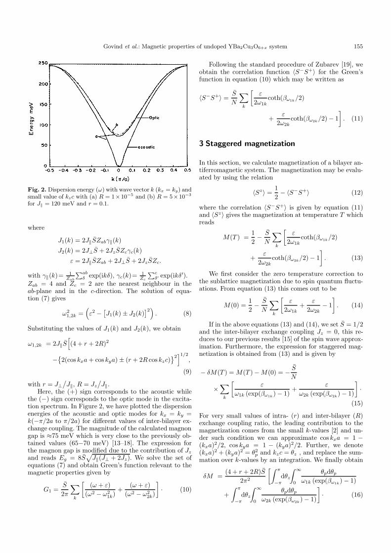
Fig. 2. Dispersion energy (ω) with wave vector k (kx = ky) andsmall value of kzc with (a) R = 1×10−5 and (b) R = 5×10−3

for J‖ = 120 meV and r = 0.1.

where

J1(k) = 2J‖SZabγ‖(k)

J2(k) = 2J⊥S + 2JzSZcγc(k)

ε = 2J‖SZab + 2J⊥S + 2JzSZc.

with γ‖(k)= 1Zab

∑abδ exp(ikδ), γc(k)= 1

Zc

∑cδ′ exp(ikδ′).

Zab = 4 and Zc = 2 are the nearest neighbour in theab-plane and in the c-direction. The solution of equa-tion (7) gives

ω21,2k =

(ε2 −

[J1(k)± J2(k)

]2). (8)

Substituting the values of J1(k) and J2(k), we obtain

ω1,2k = 2J‖S[(4 + r + 2R)2

−{

2(cos kxa+ cos kya)± (r + 2R cos kzc)}2]1/2

,

(9)

with r = J⊥/J‖, R = Jz

/J‖.

Here, the (+) sign corresponds to the acoustic whilethe (−) sign corresponds to the optic mode in the excita-tion spectrum. In Figure 2, we have plotted the dispersionenergies of the acoustic and optic modes for kx = ky =k(−π/2a to π/2a) for different values of inter-bilayer ex-change coupling. The magnitude of the calculated magnongap is ≈75 meV which is very close to the previously ob-tained values (65−70 meV) [13–18]. The expression forthe magnon gap is modified due to the contribution of Jzand reads Eg = 8S

√J‖(J⊥ + 2Jz). We solve the set of

equations (7) and obtain Green’s function relevant to themagnetic properties given by

G1 =S

2π

∑k

[(ω + ε)

(ω2 − ω21k)

+(ω + ε)

(ω2 − ω22k)

]· (10)

Following the standard procedure of Zubarev [19], weobtain the correlation function 〈S−S+〉 for the Green’sfunction in equation (10) which may be written as

〈S−S+〉 =S

N

∑k

[ε

2ω1kcoth(βω1k/2)

+ε

2ω2kcoth(βω2k/2)− 1

]. (11)

3 Staggered magnetization

In this section, we calculate magnetization of a bilayer an-tiferromagnetic system. The magnetization may be evalu-ated by using the relation

〈Sz〉 =12− 〈S−S+〉 (12)

where the correlation 〈S−S+〉 is given by equation (11)and 〈Sz〉 gives the magnetization at temperature T whichreads

M(T ) =12− S

N

∑k

[ε

2ω1kcoth(βω1k/2)

+ε

2ω2kcoth(βω2k/2)− 1

]. (13)

We first consider the zero temperature correction tothe sublattice magnetization due to spin quantum fluctu-ations. From equation (13) this comes out to be

M(0) =12− S

N

∑k

[ε

2ω1k+

ε

2ω2k− 1]. (14)

If in the above equations (13) and (14), we set S = 1/2and the inter-bilayer exchange coupling Jz = 0, this re-duces to our previous results [15] of the spin wave approx-imation. Furthermore, the expression for staggered mag-netization is obtained from (13) and is given by

− δM(T ) = M(T )−M(0) = − SN

×∑k

[ε

ω1k (exp(βω1k)− 1)+

ε

ω2k (exp(βω2k)− 1)

]·

(15)

For very small values of intra- (r) and inter-bilayer (R)exchange coupling ratio, the leading contribution to themagnetization comes from the small k-values [2] and un-der such condition we can approximate coskxa = 1 −(kxa)2/2, cos kya = 1 − (kya)2/2. Further, we denote(kxa)2 + (kya)2 = θ2

p and kzc = θz , and replace the sum-mation over k-values by an integration. We finally obtain

δM =(4 + r + 2R)S

2π2

[∫ π

−πdθz∫ ∞

0

θpdθpω1k (exp(βω1k)− 1)

+∫ π

−πdθz∫ ∞

0

θpdθpω2k (exp(βω2k)− 1)

]· (16)

156 The European Physical Journal B

I1(ω) =

�(lnR1/2 − 1)−

�ln(8 + 2r + 3R)

2− 1

�−�

(8 + 2r + 4R)1/2

2R1/2ln

����R1/2 + (8 + 2r + 4R)1/2

R1/2 − (8 + 2r + 4R)1/2

������

(4 + r + 2R)(4π2)(20)

I2(ω) =

��2− ln(2r + 4R+ 8)

2+�√

8R�

tan−1

�R1/2

2√

2

��−�

(2r + 4R)1/2

2R1/2ln

����R1/2 + (2r + 4R)1/2

R1/2 − (2r + 4R)1/2

������

(4 + r + 2R)(4π2)· (21)

We solve the above equation self consistently and calculatethe value of sublattice magnetization.

4 Neel temperature

The Neel temperature is obtained from equation (13) un-der the condition T → TN; M(T ) → 0. Thus the Neeltemperature is given by

TN =1kB

[J‖

(4 + r + 2R)I12(ω)

](17)

with I12(ω) =1N

∑k

(1ω2

1k

+1ω2

2k

)(18)

where ω1,2k is given by (9). We solve equation (18) by con-verting the summation into an integration over k-values.The analytical evaluation of I12(ω) may be written as

I12(ω) = I1(ω) + I2(ω) (19)

with

see equations (20) and (21) above.

Substituting values of I12(ω) into equation (17), wecalculate the Neel temperature for a bilayer system withintra- and inter-bilayer contributions of the exchange cou-plings.

5 Magnetic specific heat

In this section, we obtain an expression for the magneticcontribution to the specific heat using the standard pro-cedure,

CM(T ) =∂U

∂T· (22)

Here U is the internal energy of the system and at tem-perature T this is given by

U =∑k

[ω1k

(exp (βω1k)− 1)+

ω2k

(exp (βω2k)− 1)

]· (23)

Differentiating equation (23), with respect to temperatureand substituting the values of ω1k and ω2k from equa-tion (9). We get

CM(T ) = CM1(T ) + CM2(T ) (24)

CM1(T ) =∑k

[ω2

1k

kBT 2

exp (ω1k/kBT )

[exp (ω21k/kBT )− 1]2

](25)

CM2(T ) =∑k

[ω2

2k

kBT 2

exp (ω2k/kBT )

[exp (ω22k/kBT )− 1]2

]· (26)

Converting the summation over k-values into an integra-tion, the above equations (25) and (26) can be evaluated as

CM1(T ) =1

2π2

(k2

BT2

J2‖ S

2

)∫ 1

−1

θz

∫ ∞λ1

x3cosesh2xdxa

(27)

CM2(T ) =1

2π2

(k2

BT2

J2‖ S

2

)∫ 1

−1

θz

∫ ∞λ2

x3cosesh2xdxc

(28)

with

λ1 = Sb1/2/(2kBT )

λ2 = Sd1/2/(2kBT )

and,

a = 2(4 + r + 2R cos θz)b = 4R2(1− cos2 θz) + 4R(4 + r)(1− cos θz)c = 2(4− r − 2r cos θz)d = 16 + 4R2(1− cos2 θz)

+16R(1 + cos θz) + 4rR(1− cos θz).

Here, while calculating the magnetic contribution tothe specific heat at low temperatures, we have not con-sidered the temperature dependence of S. Solving theseexpressions numerically, we study the effect of intra- (r)and inter-bilayer (R) exchange coupling on the magneticspecific heat of a bilayer cuprates.

6 Results and discussion

We now present the numerical estimation of our ex-pressions for the various magnetic properties i.e. stag-gered magnetization, Neel temperature and magnetic spe-cific heat for different values of in-plane and out-of-plane

Govind et al.: Magnetic properties of undoped YBa2Cu3O6+x system 157

Fig. 3. Normalised magnetization (M(T )/M(0)) vs. temper-ature (T ) for (a) R = 1 × 10−5 and (b) R = 0.1 withJ‖ = 120 meV and r = 0.1.

(intra- and inter-bilayer) antiferromagnetic exchange cou-plings. Following earlier works [14–16], we set the in-planeexchange coupling, J‖ = 120 meV, and the intra-bilayerexchange coupling, J⊥ = 0.1J‖.

We plot reduced magnetization (M(T )/M(0)) vs. tem-perature for different values of the ratio of inter-bilayerexchange coupling to the in-plane coupling strength (R =Jz/J‖) in Figure 3. It is clear from Figure 3, that on in-creasing the strength of inter-bilayer coupling, magnetiza-tion increases. This is in accord with the experimentalobservations which suggest that inter-bilayer exchangecoupling (Jz) is essential to keep long range magnetic or-der in these systems [9–11]. It also implies that in the ab-sence of inter-bilayer exchange coupling (Jz) these bilayersbehave like a 2D-AFM system and the three-dimensionalnatures of AFM cuprates cannot be achieved. It is alsoobserved that the magnetization does not change signifi-cantly with intra-bilayer exchange coupling (J⊥).

We, next calculate the Neel temperature of these bi-layer system numerically from equation (17). Dependenceof the Neel temperature on the weak interlayer couplinghas already been discussed [8] for single layer systemsbut the effect of inter-bilayer exchange coupling in thepresence of intra-bilayer coupling has not been studied.Recently, we have studied the effect of intra-bilayer ex-change coupling on the Neel temperature [20], where thecontribution of inter-bilayer exchange coupling has beentreated phenomenologically in the model Hamiltonian.Here in Figure 4, we plot Neel temperature vs. the ratioof inter-bilayer exchange coupling to in-plane exchangecouplings (R) for J‖ = 100 meV and 120 meV, keepingthe intra-bilayer coupling fixed. It is clear from Figure 4that on increasing the strength of in-plane or inter-bilayerexchange couplings, the Neel temperature of the systemincreases. We conclude from the Figure 4 that any smallchange in inter-bilayer exchange coupling causes signifi-cant change in the Neel temperature of the system.

Fig. 4. Neel temperature (TN) vs. inter-bilayer exchange cou-pling (R) for (a) J‖ = 100 meV and (b) J‖ = 120 meV withr = 0.1.

Fig. 5. Magnetic specific heat (CM) vs. temperature (T ) for(a) R = 1 × 10−5 and (b) R = 1.0 with J‖ = 120 meV andr = 0.1.

Finally, we plot magnetic specific heat of the bilayersystem for various values of the exchange coupling fromequation (24). The expression for specific heat clearlyshows a T 2 behaviour. In Figure 5, we plot the magneticspecific heat vs. temperature for different values of the ra-tio of inter-bilayer to in-plane exchange coupling (R). It isclear from the figure that on increasing the inter-bilayerexchange coupling the magnetic contribution to specificheat increases. The magnetic specific heat shows a vari-ation higher than T 2 as inter-bilayer exchange couplingis considerable high (i.e. R = 1.0). It is also clear fromFigure 5 that at low temperatures the variation in the

158 The European Physical Journal B

magnetic specific heat due to inter-bilayer exchange cou-pling is very small. To calculate the magnetic contributionto the specific heat at low temperature it is important toconsider the temperature dependence of magnatisation, infact, magnetisation varies as T 2 at low temperatures butat high temperatures it follows a T lnT behaviour [6,15].Hence it is important to study the magnetic contributionto the specific heat at low temperature by taking the tem-perature dependence of magnetisation into account.

It can be concluded that inter-bilayer exchange cou-pling (Jz) however small, is essential to keep 3D longrange magnetic ordering in the system. Both the opticand acoustic spin wave modes contribute towards the longrange magnetic order in the presence of inter-bilayer ex-change coupling. On the other hand the magnon gap is notvery sensitive to the inter-bilayer exchange coupling (Jz).This is because of the smallness of Jz in comparison to J⊥.Moreover, one can infer from this that the magnon gap hasnothing to do with long range magnetic order in the bi-layer systems. The magnetic specific heat shows a depen-dence higher than T 2 as inter-bilayer exchange couplingis introduced. Thus, the present investigation based onRPA, clearly illustrates the importance of the role of Jz inthe magnetic dynamics of YBa2Cu3O6+x bilayer cuprates.The bilayer cuprates behave in a quite different way tosingle layered La2CuO4 system in the insulating AF mag-netic phase and it will be interesting to extend the presentcalculations to doped bilayer systems.

We are thankful to Prof. S.K. Joshi and Dr. R. Lal, NPL,for useful suggestions and discussions. The work is financiallysupported by Council of Scientific & Industrial Research, NewDelhi, India, vide Grant 31/1/(180)/2000 EMR-I and Depart-ment of Science & Technology, New Delhi, India, vide GrantNo. SP/S2/M-32/99.

References

1. A. Singh, Z. Tesanovic, H. Tang, G. Xiao, C.L. Chien, J.C.Walker, Phys. Rev. Lett. 64, 2571 (1990).

2. R.P. Singh, Z.C. Tao, M. Singh, Phys. Rev. B 46, 1244(1992), R.P. Singh, M. Singh, Phys. Rev. B 46, 14069(1992).

3. B.G. Liu, Phys. Rev. B 41, 9563 (1990).4. Ajay, S. Patra, R.S. Tripathi, Phys. Stat. Sol. (b) 188, 787

(1995).5. A. Pratap, Ajay, R.S. Tripathi, Phys. Stat. Sol. (b) 197,

453 (1996).6. P. Kopietz, Phys. Rev. Lett. 68, 3480 (1992).7. A. Auerbach, D.P. Arovas, Phys. Rev. Lett. 61, 617 (1988).8. B. Keimer, A. Aharony, A. Auerbach, R.J. Birgeneau,

A. Cassanho, Y. Endoh, R.W. Erwin, M.A. Kastner, G.Shirane, Phys. Rev. B 45, 7430 (1992).

9. J.M. Tranquada, D.E. Cox, W. Kunnmann, H. Moudden,G. Shirane, M. Suenaga, P. Zolliker, D. Vaknin, S.K. Sinha,M.S. Alvarez, A.J. Jacobson, D.C. Johnston, Phys. Rev.Lett. 60, 156 (1988).

10. J.M. Tranquada, G. Shirane, B. Keimer, S. Shamoto, M.Sato, Phys. Rev. B 40, 4503 (1989).

11. J.M. Tranquada, P.M. Gehring, G. Shirane, S. Shamoto,M. Sato, Phys. Rev. B 46, 5561 (1992).

12. S. Shamato, M. Sato, J.M. Tranquada, B.J. Sternlieb, G.Shirane, Phys. Rev. B 48, 13817 (1993).

13. R. Stern, R. Mall, J. Roos, D. Brinkmann, Phys. Rev. B52, 13817 (1995).

14. D. Reznik, P. Bourges, H.F. Fong, L.P. Regnault, J. Bossy,C. Vettier, D. Milius, I.A. Aksay, B. Keimer, Phys. Rev.B 53, R14741 (1996).

15. A. Pratap, Govind, R.S. Tripathi, Phys. Rev. B 60, 6775(1999).

16. A.J. Millis, H. Monien, Phys. Rev. B 54, 16172 (1996).17. A.J. Millis, H. Monien, Phys. Rev. B 50, 16606 (1994).18. A. Du, G.M. Li, G.Z. Wei, Phys. Stat Sol. (b) 203, 517

(1997).19. D.N. Zubarev, Sov. Phys. Usp. 3, 302 (1960).20. Govind, A. Pratap, Ajay, R.S. Tripathi, Pramana 54, 423

(2000).