magnetic field of helmholtz coils and magnetic moment - group 4 - 24,25 sept 2012 (1)
TRANSCRIPT

Magnetic Field of Helmholtz Coils and Magnetic Moment
Alexandra Crai, Alexandru PopaAdvanced Physics A+B Laboratory Course I
Jacobs University Bremen - Fall 2012
Group 4
Date of execution: September, 24-25, 2012
Abstract
The magnetic field created by Helmholtz coils was studied in this experiment.In the first part, the value of Bz was measured for different radii r. The experimentwas repeated for the radial flux Br. It was proven that B decreased with increasingz-position and increased as r approached R. Next, two coils were used to determinethe field’s distribution between them for different separations a. As expected, whena = R the field inside was constant. The axial and radial components’ of themagnetic field as functions of z and r when a = R were next investigated. Last,the torque due to the magnetic moment in a small conductor coil was determinedas a function of strength of both the magnetic field and magnetic moment and ofthe angle between them. A linear dependence was proven for all three cases.
1

Contents
1 Introduction and Theory 3
2 Experimental Set-up and Procedure 52.1 Magnetic field of a single coil . . . . . . . . . . . . . . . . . . . . . . . . 52.2 Magnetic field of two parallel coils . . . . . . . . . . . . . . . . . . . . . . 62.3 Magnetic moment in a field of a Helmholtz coil arrangement . . . . . . . 8
3 Results and Data Analysis 93.1 Magnetic Field of a Single Coil . . . . . . . . . . . . . . . . . . . . . . . 9
3.1.1 Determination of Bz along the z-axis for different radii r . . . . . 93.1.2 Determination of Br along the r-axis for different z . . . . . . . . 13
3.2 Magnetic Field of Two Parallel Coils . . . . . . . . . . . . . . . . . . . . 193.2.1 Determination of Bz along the z-axis for a separation of a = R/2 . 203.2.2 Determination of Bz along the z-axis for a separation of a = R . . 223.2.3 Determination of Bz along the z-axis for a separation of a = 2R . 233.2.4 Comparison between a = R/2, a = R and a = 2R . . . . . . . . . 263.2.5 Determination of Bz of a Helmholtz arrangement for 5 different radii 263.2.6 Determination of Br of a Helmholtz arrangement for 5 different radii 30
3.3 Magnetic moment in a field of a Helmholtz coil arrangement . . . . . . . 383.3.1 Torque as a function of the strength of the magnetic field . . . . . 383.3.2 Torque as a function of the angle between the magnetic field and
magnetic moment . . . . . . . . . . . . . . . . . . . . . . . . . . . 403.3.3 Torque as a function of the strength of the magnetic moment . . . 44
Bibliography 45
2

1 Introduction and Theory
In this experiment, the magnetic field in coils and the torque experienced by a smallcurrent loop with a magnetic moment in a magnetic field were examined. First, a steadycurrent was flowing through a single coil and the magnetic field along the z-axis wasmeasured at different points on that axis. Then, the radial flux density, perpendicularto z-axis, was measured at different distances from the center of the coil. In the secondpart, the magnetic field of a system of two coils was analysed. For different distancesbetween the two coils, namely one half, one and double of the radius of one coil, themagnetic flux along the z-axis was measured as a function of the distance z from the cen-ter of the coil. Next, the distance between the coil was kept constant and the magneticflux density as a function the distance z for different distances r from the symmetry axiswas measured. This was repeated for the radial flux density along the z-axis in depen-dence of the distance r to the symmetry axis. In the last part, the torque experiencedby a small conductor loop carrying a current in an uniform magnetic field was measuredas a function of the strength of the magnetic field, of the angle between the magneticfield and the magnetic moment and of the strength of the magnetic moment was recorded.
The Biot-Savart’s Law is one of the most used one for this experiment [1].It gives the
strength of the magnetic d−→B field on a certain conductor element d
−→l due to a current I:
d−→B =
Iµ0
4π
d−→l ×−→rr3
(1)
Here, −→r is the vector that points from the point where the magnetic field d−→B is
measured to the conductor element d−→l . µ0 is the magnetic permeability. From the cross
product, the magnetic field is perpendicular on both dl and dr vectors. Let R be theradius of the coil and Z the distance perpendicular to the plane of the coil. Therefore:
r2 = R2 + Z2 (2)
The magnetic fields along the axis of symmetry will therefore be:
dB =I
4πr2· dl =
Iµ0
4π· dl
R2 + Z2(3)
Thus, the field lines are rotationally symmetric along the z-axis. The radial component ofthe magnetic field is zero since all the contributions from the conductor elements cancelout. Hence, the magnetic field is completely given by the z-component. It is computedby integration over all the conductor elements contributing to the field:
B(z, r = 0) = Bz(z, r = 0) =Iµ0
2· R2
(R2 + Z2)3/2(4)
The equation above gives the magnetic field per turn of a coil [1]. For a coil with N turns,the total magnetic flux density along the symmetry axis of the system formed from twosuch coils at distance a apart is given by:
B(z, r = 0) =µ0IN
2R·[
1
(1 + A21)
3/2+
1
(1 + A22)
3/2
](5)
3
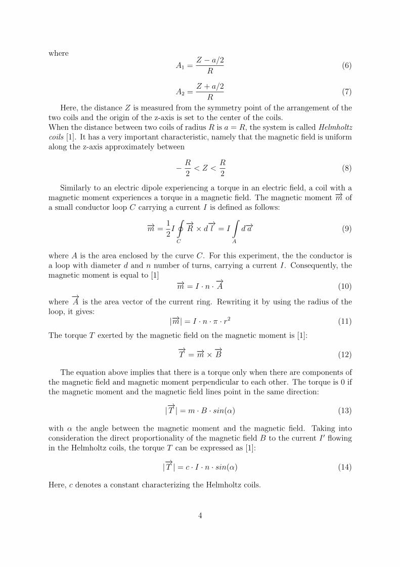
where
A1 =Z − a/2
R(6)
A2 =Z + a/2
R(7)
Here, the distance Z is measured from the symmetry point of the arrangement of thetwo coils and the origin of the z-axis is set to the center of the coils.When the distance between two coils of radius R is a = R, the system is called Helmholtzcoils [1]. It has a very important characteristic, namely that the magnetic field is uniformalong the z-axis approximately between
− R
2< Z <
R
2(8)
Similarly to an electric dipole experiencing a torque in an electric field, a coil with amagnetic moment experiences a torque in a magnetic field. The magnetic moment −→m ofa small conductor loop C carrying a current I is defined as follows:
−→m =1
2I
∮C
−→R × d
−→l = I
∫A
d−→a (9)
where A is the area enclosed by the curve C. For this experiment, the the conductor isa loop with diameter d and n number of turns, carrying a current I. Consequently, themagnetic moment is equal to [1]
−→m = I · n ·−→A (10)
where−→A is the area vector of the current ring. Rewriting it by using the radius of the
loop, it gives:|−→m| = I · n · π · r2 (11)
The torque T exerted by the magnetic field on the magnetic moment is [1]:
−→T = −→m ×
−→B (12)
The equation above implies that there is a torque only when there are components ofthe magnetic field and magnetic moment perpendicular to each other. The torque is 0 ifthe magnetic moment and the magnetic field lines point in the same direction:
|−→T | = m ·B · sin(α) (13)
with α the angle between the magnetic moment and the magnetic field. Taking intoconsideration the direct proportionality of the magnetic field B to the current I ′ flowingin the Helmholtz coils, the torque T can be expressed as [1]:
|−→T | = c · I · n · sin(α) (14)
Here, c denotes a constant characterizing the Helmholtz coils.
4

2 Experimental Set-up and Procedure
2.1 Magnetic field of a single coil
In this part of the experiment, the magnetic field generated by a single coil was measured.The coil was placed on the working table and was connected in series to a power gener-ator and an ammeter. From the ammeter the current flowing through the coil could bedetermined. The radius of the coil was determined by measuring the coil’s external andinternal diameters, which were noted in the lab book. These values were then averaged todetermine the radius of the coil. An axial Hall probe was used to measure the magneticflux created by the coil. The probe was held by a support rod and was placed on ameter scale which was clamped to the working table. This way, the position of the proberelative to the meter scale could be read, which allowed for calculation of the distancebetween the coil and the point at which the magnetic flux measurement was done. Beforethe measurements could begin, the probe was placed far from conducting elements andwas calibrated to a value of 0 mT such that external magnetic fields would not affect themeasurements. This was done before every part of the experiment. Next, the Hall probewas placed in the center of the coil and its position on the meter scale was recorded inthe lab book. A meter scale was placed next to the coil in radial direction, such that thecenter of the coil’s position relative to the position of the Hall probe could be measuredand noted in the lab book. The probe was moved in the z-direction and the values forthe magnetic flux and the corresponding positions of the probe relative to the coil weremeasured. After each set of measurements was done, the coil’s position was changed,such that the distance r between the probe and the coil’s central axis was different. Theset-up for this part of the experiment can be observed in Figure 1.
Figure 1: Experimental set-up for determination of the magnetic field created in z-direction by
a coil
5

Next, the same set-up was used, but the Hall probe was rotated 90◦, such that theradial component of the magnetic field could be measured. Again, the probe was placedat several distances on the z-axis and each set of measurements was repeated at differentdistances r from the coil’s axis. The set-up for this part of the experiment can be observedin Figure 2.
Figure 2: Experimental set-up for determination of the magnetic field created in radial direction
by a coil
2.2 Magnetic field of two parallel coils
In this part of the experiment the magnetic field created by two parallel coils was mea-sured. The two coils were connected in series to a power generator and to an ammeter. Asimilar set-up as in the case of a single coil was used. Several separations a between thecoils were used: a = R
2, a = R and a = 2R, where R was the radius of the identical coils.
In this case, the axial magnetic field was measured as a function of separation betweenthe probe and the first coil. In the next part of the experiment the coils were placedin a Helmholtz arrangement, a = R. The magnetic flux pointing in the z-direction wasmeasured for several distances r from the coils’ central axis as a function of distance fromthe coils. The distance z from the coils was read from the meter scale placed under theprobe and the position of the Helmholtz coils was varied on the meter scale perpendicularto their central axis. The distances from the central axis were chosen in such a way thatthe radius of the cylinder inside the Helmholtz arrangement where the axial magneticfield can be approximated as constant would be obvious. The set-up for this part of theexperiment can be observed in Figure 3.
Next, the Helmholtz coils were turned 90◦ such that the radial component Br of themagnetic flux could be measured for different distances r from the probe to the axial
6

Figure 3: Experimental set-up for determination of the magnetic field created in the z-direction
by two coils
center of the two coils. For every set of measurements, the probe was moved in the z-direction and its position relative to the first coil was recorded. The set-up for this partof the experiment can be observed in Figure 4.
Figure 4: Experimental set-up for determination of the magnetic field created in radial direction
by two coils
7

2.3 Magnetic moment in a field of a Helmholtz coil arrangement
In this final part of the experiment the torque experienced by a current loop in a magneticfield created by a Helmholtz arrangement was measured as a function of the strengthof the magnetic field, the initial angle between the magnetic field and the magneticmoment, and the strength of the magnetic moment. The same set-up as in the previouspart was used. To measure the torque, a torsion dynamometer was placed on a supportrod above the Helmholtz arrangement. A wire loop with 3 turns was connected to thetorsion dynamometer and in series to an ammeter and a power generator. This way,the current flowing through the wire loop could be determined by the ammeter. Next,the dynamometer was calibrated to the zero point while there was no current flowingthrough the coils and the loop. This was done by turning the knob on the top of thedynamometer to the 0 position. When there was a torque acting on the current loop,the knob changed position which allowed for the force to be read off the dynamometer.Next, the measurements could begin. First, the torque was determined as a function ofthe magnetic field generated by the coils. In this case, the angle between the magneticmoment and the magnetic field was kept constant. The strength of the magnetic momentwas also kept constant. Next, the torque was determined as a function of the initialangle between the magnetic moment and the field, while the magnetic field and momentwere kept at constant values. The angle was changed in steps of 15◦ and it was readfrom the divisions on the loop. Finally, the torque dependence on the strength of themagnetic moment was measured. The magnetic moment was varied and the torque wasmeasured for constant values of the magnetic field and angle between field and moment.The experimental set-up for this part of the experiment can be observed in Figure 5.
Figure 5: Experimental set-up for determination of torque as a function of field, angle and
magnetic moment
8

3 Results and Data Analysis
3.1 Magnetic Field of a Single Coil
3.1.1 Determination of Bz along the z-axis for different radii r
Data Collection
First, the radius of the coil had to be determined. For this, the internal and externaldiameters of the coil were averaged using Equation 15:
R =1
2· Dout +Din
2(15)
where the values for the two diameters were determined to be Dout = 41.6 cm andDin = 38.0 cm. By plugging in the respective values in Equation 15, the value for thecoil’s radius was determined:
R = 19.9 cm
Next, the initial position of the Hall probe for which the relative position to the coilwas measured to be 0 was determined to be z′ = 26 cm. The value for the relativeposition of the Hall probe was determined using Equation 16:
z = zmeas − z′ (16)
where zmeas was the value read from the meter scale. For this part of the experiment,the current flowing through the coil was kept at a constant value of
I = 2.75 A
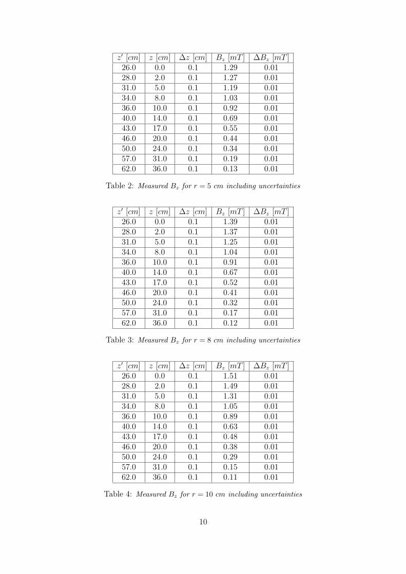
The measurements were performed for different values of r and z and the gathered datais presented in Tables 1, 2, 3, 4, 5 and 6. The values are presented along with theiruncertainties which were taken from the accuracies of the measurement devices: the tes-lameter and the ammeter. Each set of measurements was performed for a correspondingvalue: r = 0 cm, r = 5 cm, r = 8 cm, r = 10 cm, r = 14 cm and r = 17 cm.
z′ [cm] z [cm] ∆z [cm] Bz [mT ] ∆Bz [mT ]26.0 0.0 0.1 1.25 0.0128.0 2.0 0.1 1.24 0.0131.0 5.0 0.1 1.15 0.0134.0 8.0 0.1 1.02 0.0136.0 10.0 0.1 0.91 0.0140.0 14.0 0.1 0.70 0.0143.0 17.0 0.1 0.57 0.0146.0 20.0 0.1 0.45 0.0150.0 24.0 0.1 0.36 0.0157.0 31.0 0.1 0.20 0.0162.0 36.0 0.1 0.15 0.01
Table 1: Measured Bz for r = 0 cm including uncertainties
9
z′ [cm] z [cm] ∆z [cm] Bz [mT ] ∆Bz [mT ]26.0 0.0 0.1 1.29 0.0128.0 2.0 0.1 1.27 0.0131.0 5.0 0.1 1.19 0.0134.0 8.0 0.1 1.03 0.0136.0 10.0 0.1 0.92 0.0140.0 14.0 0.1 0.69 0.0143.0 17.0 0.1 0.55 0.0146.0 20.0 0.1 0.44 0.0150.0 24.0 0.1 0.34 0.0157.0 31.0 0.1 0.19 0.0162.0 36.0 0.1 0.13 0.01
Table 2: Measured Bz for r = 5 cm including uncertainties
z′ [cm] z [cm] ∆z [cm] Bz [mT ] ∆Bz [mT ]26.0 0.0 0.1 1.39 0.0128.0 2.0 0.1 1.37 0.0131.0 5.0 0.1 1.25 0.0134.0 8.0 0.1 1.04 0.0136.0 10.0 0.1 0.91 0.0140.0 14.0 0.1 0.67 0.0143.0 17.0 0.1 0.52 0.0146.0 20.0 0.1 0.41 0.0150.0 24.0 0.1 0.32 0.0157.0 31.0 0.1 0.17 0.0162.0 36.0 0.1 0.12 0.01
Table 3: Measured Bz for r = 8 cm including uncertainties
z′ [cm] z [cm] ∆z [cm] Bz [mT ] ∆Bz [mT ]26.0 0.0 0.1 1.51 0.0128.0 2.0 0.1 1.49 0.0131.0 5.0 0.1 1.31 0.0134.0 8.0 0.1 1.05 0.0136.0 10.0 0.1 0.89 0.0140.0 14.0 0.1 0.63 0.0143.0 17.0 0.1 0.48 0.0146.0 20.0 0.1 0.38 0.0150.0 24.0 0.1 0.29 0.0157.0 31.0 0.1 0.15 0.0162.0 36.0 0.1 0.11 0.01
Table 4: Measured Bz for r = 10 cm including uncertainties
10
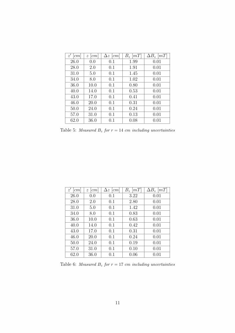
z′ [cm] z [cm] ∆z [cm] Bz [mT ] ∆Bz [mT ]26.0 0.0 0.1 1.99 0.0128.0 2.0 0.1 1.91 0.0131.0 5.0 0.1 1.45 0.0134.0 8.0 0.1 1.02 0.0136.0 10.0 0.1 0.80 0.0140.0 14.0 0.1 0.53 0.0143.0 17.0 0.1 0.41 0.0146.0 20.0 0.1 0.31 0.0150.0 24.0 0.1 0.24 0.0157.0 31.0 0.1 0.13 0.0162.0 36.0 0.1 0.08 0.01
Table 5: Measured Bz for r = 14 cm including uncertainties
z′ [cm] z [cm] ∆z [cm] Bz [mT ] ∆Bz [mT ]26.0 0.0 0.1 3.22 0.0128.0 2.0 0.1 2.80 0.0131.0 5.0 0.1 1.42 0.0134.0 8.0 0.1 0.83 0.0136.0 10.0 0.1 0.63 0.0140.0 14.0 0.1 0.42 0.0143.0 17.0 0.1 0.31 0.0146.0 20.0 0.1 0.24 0.0150.0 24.0 0.1 0.19 0.0157.0 31.0 0.1 0.10 0.0162.0 36.0 0.1 0.06 0.01
Table 6: Measured Bz for r = 17 cm including uncertainties
11

Error Calculation
The uncertainty in the measurement of the radius R of the coil was next calculated. Theerrors in the measurements of ∆Dout and ∆Din were taken from the accuracy of the meterscale as follows:
∆Din = ∆Dout = 0.1 cm
The uncertainty in R was calculated using the propagated error formula:
∆R =
√(∂R
∂Dout
·∆Dout
)2
+
(∂R
∂Din
·∆Din
)2
=1
4·√
∆D2out + ∆D2
in (17)
After plugging in the respective values in Equation 17, the uncertainty in R wasdetermined:
∆R = 0.1 cm
The final value for the coil’s radius was then determined:
R = (19.9± 0.1) cm
The errors in the measurement of the probe and coil’s positions, magnetic flux andcurrent flowing through the coil were also taken from the accuracies of the measurementinstruments:
∆z = ∆z′ = ∆zmeas = ∆r = 0.1 cm
∆I = 0.01 A
∆B = 0.01 mT
Data evaluation
The data gathered for this part of the experiment was next plotted in Figures 6, 7, 8,9, 10 and 11. The respective uncertainties were also included on the plots.
From the results, a qualitative description of the magnetic field generated by a singlecoil with respect to distance could be made.
Discussion and Conclusion
From the plots it can be observed that the value for the axial component of the magneticfield increases as one approaches the coil, as expected. This increase is smaller whenthe measurement takes place along the central axis of the coil and larger when the mea-surement is done at a certain distance from the axis. This is due to the fact that onlythe magnetic field in the axial direction was measured; when the probe was placed at acertain distance r, the field components in the radial direction no longer cancelled eachother out, fact that meant that the axial component of the field had to be smaller inorder to maintain the total magnitude of the magnetic field at that position constant.
12

Figure 6: Bz for r = 0 cm
Figure 7: Bz for r = 5 cm
3.1.2 Determination of Br along the r-axis for different z
Data Collection
Next, the radial flux density Br of the single coil was determined for several distancesz = 0 cm, z = 3.5 cm, z = 5.5 cm and z = 7.5 cm from the plane containing the coil.The measurements were done at different distances r from the axial center of the coil.The current in the coil was kept at a constant value:
I = 2.75 A
13
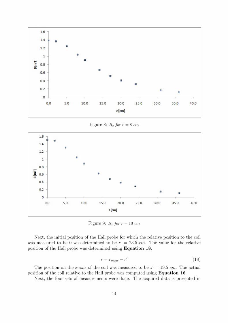
Figure 8: Bz for r = 8 cm
Figure 9: Bz for r = 10 cm
Next, the initial position of the Hall probe for which the relative position to the coilwas measured to be 0 was determined to be r′ = 23.5 cm. The value for the relativeposition of the Hall probe was determined using Equation 18.
r = rmeas − r′ (18)
The position on the z-axis of the coil was measured to be z′ = 19.5 cm. The actualposition of the coil relative to the Hall probe was computed using Equation 16.
Next, the four sets of measurements were done. The acquired data is presented in
14

Figure 10: Bz for r = 14 cm
Figure 11: Bz for r = 17 cm
Tables 7, 8, 9 and 10.
Error Calculation
The errors in the measurement of the probe and coil’s positions, magnetic flux and cur-rent flowing through the coil were also taken from the accuracies of the measurementinstruments.
15

rmeas [cm] r [cm] ∆r [cm] Br [mT ] ∆Br [mT ]23.5 0.0 0.1 0.00 0.0126.0 2.5 0.1 0.01 0.0128.0 4.5 0.1 0.02 0.0131.0 7.5 0.1 0.04 0.0133.0 9.5 0.1 0.07 0.0135.0 11.5 0.1 0.12 0.0137.0 13.5 0.1 0.23 0.0139.0 15.5 0.1 0.47 0.0141.0 17.5 0.1 1.56 0.0141.5 18.0 0.1 2.24 0.0142.0 18.5 0.1 3.36 0.0143.0 19.5 0.1 6.08 0.0144.0 20.5 0.1 4.62 0.0146.0 22.5 0.1 0.89 0.0148.0 24.5 0.1 0.35 0.01
Table 7: Measured Br for z = 0 cm including uncertainties
rmeas [cm] r [cm] ∆r [cm] Br [mT ] ∆Br [mT ]23.5 0.0 0.1 0.00 0.0126.0 2.5 0.1 0.03 0.0128.0 4.5 0.1 0.07 0.0131.0 7.5 0.1 0.13 0.0133.0 9.5 0.1 0.19 0.0135.0 11.5 0.1 0.29 0.0137.0 13.5 0.1 0.49 0.0139.0 15.5 0.1 0.89 0.0141.0 17.5 0.1 1.85 0.0141.5 18.0 0.1 2.23 0.0142.0 18.5 0.1 2.61 0.0143.0 19.5 0.1 3.06 0.0144.0 20.5 0.1 2.68 0.0146.0 22.5 0.1 1.22 0.0148.0 24.5 0.1 0.53 0.01
Table 8: Measured Br for z = 3.5 cm including uncertainties
16

rmeas [cm] r [cm] ∆r [cm] Br [mT ] ∆Br [mT ]23.5 0.0 0.1 0.00 0.0126.0 2.5 0.1 0.06 0.0128.0 4.5 0.1 0.09 0.0131.0 7.5 0.1 0.18 0.0133.0 9.5 0.1 0.27 0.0135.0 11.5 0.1 0.41 0.0137.0 13.5 0.1 0.62 0.0139.0 15.5 0.1 0.96 0.0141.0 17.5 0.1 1.37 0.0141.5 18.0 0.1 1.46 0.0142.0 18.5 0.1 1.53 0.0143.0 19.5 0.1 1.58 0.0144.0 20.5 0.1 1.48 0.0146.0 22.5 0.1 1.03 0.0148.0 24.5 0.1 0.62 0.01
Table 9: Measured Br for z = 5.5 cm including uncertainties
rmeas [cm] r [cm] ∆r [cm] Br [mT ] ∆Br [mT ]23.5 0.0 0.1 0.00 0.0126.0 2.5 0.1 0.06 0.0128.0 4.5 0.1 0.12 0.0131.0 7.5 0.1 0.22 0.0133.0 9.5 0.1 0.32 0.0135.0 11.5 0.1 0.44 0.0137.0 13.5 0.1 0.61 0.0139.0 15.5 0.1 0.81 0.0141.0 17.5 0.1 0.99 0.0141.5 18.0 0.1 1.02 0.0142.0 18.5 0.1 1.04 0.0143.0 19.5 0.1 1.05 0.0144.0 20.5 0.1 0.99 0.0146.0 22.5 0.1 0.80 0.0148.0 24.5 0.1 0.56 0.01
Table 10: Measured Br for z = 7.5 cm including uncertainties
17
∆z = ∆z′ = ∆zmeas = ∆r = ∆r′ = ∆rmeas = 0.1 cm
∆I = 0.01 A
∆B = 0.01 mT
Data Evaluation
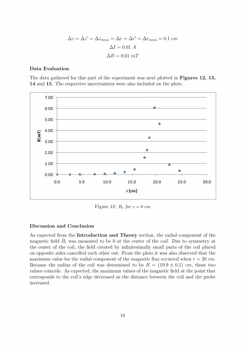
The data gathered for this part of the experiment was next plotted in Figures 12, 13,14 and 15. The respective uncertainties were also included on the plots.
Figure 12: Br for z = 0 cm
Discussion and Conclusion
As expected from the Introduction and Theory section, the radial component of themagnetic field Br was measured to be 0 at the center of the coil. Due to symmetry atthe center of the coil, the field created by infinitesimally small parts of the coil placedon opposite sides cancelled each other out. From the plots it was also observed that themaximum value for the radial component of the magnetic flux occurred when r = 20 cm.Because the radius of the coil was determined to be R = (19.9 ± 0.1) cm, these twovalues coincide. As expected, the maximum values of the magnetic field at the point thatcorresponds to the coil’s edge decreased as the distance between the coil and the probeincreased.
18
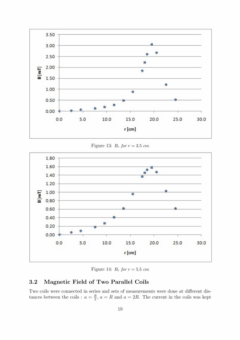
Figure 13: Br for r = 3.5 cm
Figure 14: Br for r = 5.5 cm
3.2 Magnetic Field of Two Parallel Coils
Two coils were connected in series and sets of measurements were done at different dis-tances between the coils : a = R
2, a = R and a = 2R. The current in the coils was kept
19

Figure 15: Br for r = 7.5 cm
at a constant value of I = 2.75 A while every set of measurements was done.
3.2.1 Determination of Bz along the z-axis for a separation of a = R/2
Data Collection and Error Calculation
The value of z′ at which the Hall probe was in the center of the first coil was determinedto be z′ = 16 cm. By using Equation 16 the relative position of the probe to the firstcoil was determined. The gathered data including uncertainties is presented in Table11.
The uncertainties of the gathered data were taken from the accuracies of the measuringinstruments. Because distances were measured with a meter scale and the magnetic fluxwith a teslameter, the uncertainties in the measurements of z and Bz became
∆zmeas = ∆z = 0.1 cm
∆Bz = 0.1 mT
Data Evaluation
The gathered data for this section was plotted in Figure 16. Since the coils were placedat a distance of a = R/2, by plugging in the value for R into the aforementioned formula,the value at which the second coil was computed:
a = (10.0± 0.1) cm
The uncertainty for a was taken from the accuracy of the meter scale.
20

zmeas [cm] z [cm] ∆z [cm] Bz [mT ] ∆Bz [mT ]16.0 0.0 0.1 2.09 0.0117.0 1.0 0.1 2.16 0.0118.0 2.0 0.1 2.20 0.0119.0 3.0 0.1 2.23 0.0121.0 5.0 0.1 2.26 0.0122.0 6.0 0.1 2.26 0.0123.0 7.0 0.1 2.25 0.0124.0 8.0 0.1 2.22 0.0125.0 9.0 0.1 2.18 0.0126.0 10.0 0.1 2.13 0.0127.0 11.0 0.1 2.08 0.0128.0 12.0 0.1 2.01 0.0129.0 13.0 0.1 1.93 0.0130.0 14.0 0.1 1.85 0.01
Table 11: Measured Bz for a = R/2 including uncertainties
The black vertical line in Figure 16 represents the position of the second coil relativeto the first coil.
Figure 16: Bz for a = R/2 including uncertainties
21

Discussion and Conclusion
Measurements were also done at distances larger than the separation of the two coils. Asexpected, the value of the magnetic field in the z-direction starts dropping for distanceslarger than a. Also, it can be seen that the magnetic field between the two coils wasnot constant, since the coils were not placed in a Helmholtz arrangement. This case wasinvestigated in the next subsection.
3.2.2 Determination of Bz along the z-axis for a separation of a = R
Data Collection and Error Calculation
The value of z′ at which the Hall probe was in the center of the first coil was determinedto be z′ = 6 cm. By using Equation 16 the relative position of the probe to the first coilwas determined. The gathered data including uncertainties is presented in Table 12.
z′ [cm] z [cm] ∆z [cm] Bz [mT ] ∆Bz [mT ]6.0 0.0 0.1 1.67 0.018.0 2.0 0.1 1.74 0.0110.0 4.0 0.1 1.77 0.0112.0 6.0 0.1 1.79 0.0114.0 8.0 0.1 1.79 0.0116.0 10.0 0.1 1.79 0.0118.0 12.0 0.1 1.80 0.0120.0 14.0 0.1 1.79 0.0122.0 16.0 0.1 1.79 0.0124.0 18.0 0.1 1.76 0.0126.0 20.0 0.1 1.70 0.0128.0 22.0 0.1 1.62 0.0130.0 24.0 0.1 1.51 0.0132.0 26.0 0.1 1.38 0.0134.0 28.0 0.1 1.26 0.01
Table 12: Measured Bz for a = R including uncertainties
The uncertainties of the gathered data were taken from the accuracies of the measuringinstruments. Because distances were measured with a meter scale and the magnetic fluxwith a teslameter, the uncertainties in the measurements of z and Bz became
∆zmeas = ∆z = 0.1 cm
∆Bz = 0.1 mT
Data Evaluation
The gathered data for this section was plotted in Figure 17. Since the coils were placedat a distance of a = R, by plugging in the value for R into the aforementioned formula,the value at which the second coil was placed:
a = (19.9± 0.1) cm
22
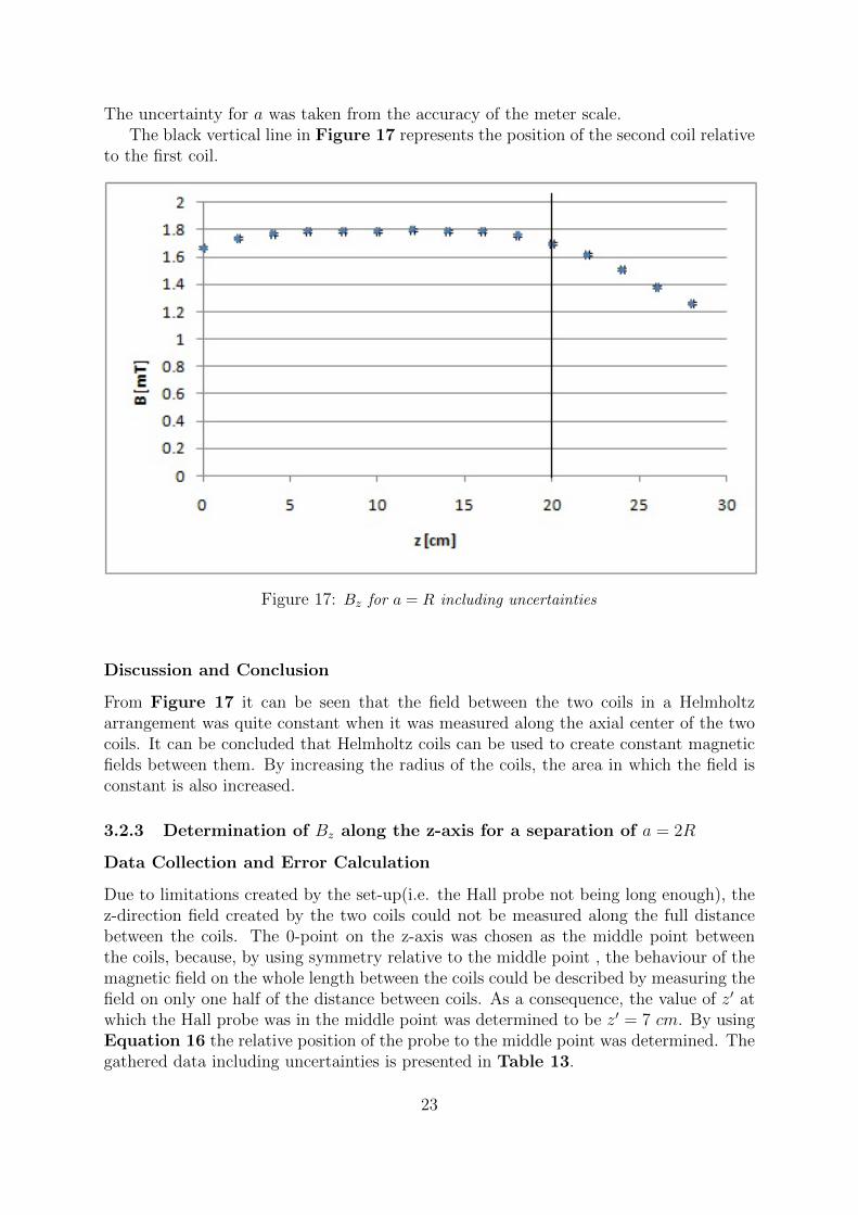
The uncertainty for a was taken from the accuracy of the meter scale.The black vertical line in Figure 17 represents the position of the second coil relative
to the first coil.
Figure 17: Bz for a = R including uncertainties
Discussion and Conclusion
From Figure 17 it can be seen that the field between the two coils in a Helmholtzarrangement was quite constant when it was measured along the axial center of the twocoils. It can be concluded that Helmholtz coils can be used to create constant magneticfields between them. By increasing the radius of the coils, the area in which the field isconstant is also increased.
3.2.3 Determination of Bz along the z-axis for a separation of a = 2R
Data Collection and Error Calculation
Due to limitations created by the set-up(i.e. the Hall probe not being long enough), thez-direction field created by the two coils could not be measured along the full distancebetween the coils. The 0-point on the z-axis was chosen as the middle point betweenthe coils, because, by using symmetry relative to the middle point , the behaviour of themagnetic field on the whole length between the coils could be described by measuring thefield on only one half of the distance between coils. As a consequence, the value of z′ atwhich the Hall probe was in the middle point was determined to be z′ = 7 cm. By usingEquation 16 the relative position of the probe to the middle point was determined. Thegathered data including uncertainties is presented in Table 13.
23

z′ [cm] z [cm] ∆z [cm] Bz [mT ] ∆Bz [mT ]2.0 -5.0 0.1 0.94 0.013.0 -4.0 0.1 0.93 0.014.0 -3.0 0.1 0.91 0.015.0 -2.0 0.1 0.90 0.016.0 -1.0 0.1 0.90 0.017.0 0.0 0.1 0.89 0.018.0 1.0 0.1 0.89 0.019.0 2.0 0.1 0.89 0.0110.0 3.0 0.1 0.90 0.0112.0 5.0 0.1 0.92 0.0114.0 7.0 0.1 0.98 0.0116.0 9.0 0.1 1.06 0.0118.0 11.0 0.1 1.13 0.0120.0 13.0 0.1 1.20 0.0123.0 16.0 0.1 1.31 0.0126.0 19.0 0.1 1.35 0.0129.0 22.0 0.1 1.31 0.0132.0 25.0 0.1 1.21 0.0135.0 28.0 0.1 1.05 0.0138.0 31.0 0.1 0.89 0.01
Table 13: Measured Bz for a = 2R including uncertainties
24

The uncertainties of the gathered data were taken from the accuracies of the measuringinstruments. Because distances were measured with a meter scale and the magnetic fluxwith a teslameter, the uncertainties in the measurements of z and Bz became
∆zmeas = ∆z = 0.1 cm
∆Bz = 0.1 mT
Data Evaluation
The gathered data for this section was plotted in Figure 18.The black vertical line in Figure 18 represents the position of the second coil relative
to the middle point between the coils, which was taken as the origin on the z-axis.
Figure 18: Bz for a = 2R including uncertainties
Discussion and Conclusion
Again, since the coils were no longer placed in a Helmholtz arrangement, the magneticfield between them was no longer constant. This can be observed in Figure 18, wherethe lowest value for the z-direction field was registered in the middle point between thecoils. As the probe approached the coils, the value for the field began increasing. As aconclusion, the field could be approximated as constant only on short distances, a fewcentimetres to both sides of the middle point between the coils.
25

3.2.4 Comparison between a = R/2, a = R and a = 2R
The data points gathered from the three cases investigated were all plotted in Figure19, fact that facilitated the final comparison between the three different arrangements.
Figure 19: Comparison between cases a = R/2, a = R and a = 2R
Consequently, by analysing Figure 19, it can be observed that the magnetic fieldbetween the coils can be assumed to be constant only when the coils were in a Helmholtzarrangement. This is explained by the superposition of the fields generated by each coil.
3.2.5 Determination of Bz of a Helmholtz arrangement for 5 different radii
The same set-up as in the previous section was used. The coils were placed in a Helmholtzarrangement, with a distance between them of a = R = (19.9±0.1) cm. Sets of measure-ments were done at different distances r from the axial center of the coils. The currentin the coils was kept at a constant value of I = 2.75 A while every set of measurementswas done. The position at which z = 0 was taken as the position of the first coil in thearrangement.
Data Collection and Error Calculation
As in the previous section, the position at which r was 0 cm was measured with a meterscale to be r′ = (17.0 ± 0.1) cm. The values of r for which each set of measurementswas done were computed using Equation 18. The position at which z was 0 cm wasdetermined to be z = (6.0± 0.1) cm. The values of z were determined using Equation16. The uncertainties in the measurements of r, r′, rmeas, z, z′, zmeas were taken from
26

the accuracies of the meter scales used. The errors in the measurements of I and Bz weretaken from the accuracies of the ammeter and the teslameter, respectively. Thus:
∆z = ∆z′ = ∆zmeas = 0.1 cm
∆r = ∆r′ = ∆rmeas = 0.1 cm
∆I = 0.1 A
∆Bz = 0.01 mT
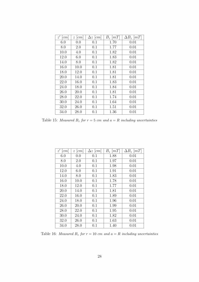
The gathered data including their uncertainties is presented in Tables 14, 15, 16,17 and 18.
z′ [cm] z [cm] ∆z [cm] Bz [mT ] ∆Bz [mT ]6.0 0.0 0.1 1.66 0.018.0 2.0 0.1 1.72 0.0110.0 4.0 0.1 1.76 0.0112.0 6.0 0.1 1.79 0.0114.0 8.0 0.1 1.79 0.0116.0 10.0 0.1 1.79 0.0118.0 12.0 0.1 1.80 0.0120.0 14.0 0.1 1.79 0.0122.0 16.0 0.1 1.80 0.0124.0 18.0 0.1 1.77 0.0126.0 20.0 0.1 1.74 0.0128.0 22.0 0.1 1.67 0.0130.0 24.0 0.1 1.57 0.0132.0 26.0 0.1 1.45 0.0134.0 28.0 0.1 1.32 0.01
Table 14: Measured Bz for r = 0 cm and a = R including uncertainties
Data Evaluation
The gathered data along with the uncertainties were plotted in Figures 20, 21, 22, 23and 24.
Discussion and Conclusion
The specific values for r were chosen in such a way that the radius of the cylinder insidethe Helmholtz arrangement where the magnetic field was constant could be observed.As it can be seen from Figures 20, 21, 22, 23 and 24, once the radius r had a valuelarger than 5 cm the magnetic field inside the coils could no longer be approximated asconstant. As a consequence, a cylinder of radius r = 5 cm centred with the coils’ z-axiscould be imagined inside the Helmholtz arrangement. Inside this cylinder the magneticfield in z-direction can safely be assumed to be constant.
27
z′ [cm] z [cm] ∆z [cm] Bz [mT ] ∆Bz [mT ]6.0 0.0 0.1 1.70 0.018.0 2.0 0.1 1.77 0.0110.0 4.0 0.1 1.82 0.0112.0 6.0 0.1 1.83 0.0114.0 8.0 0.1 1.82 0.0116.0 10.0 0.1 1.81 0.0118.0 12.0 0.1 1.81 0.0120.0 14.0 0.1 1.81 0.0122.0 16.0 0.1 1.83 0.0124.0 18.0 0.1 1.84 0.0126.0 20.0 0.1 1.81 0.0128.0 22.0 0.1 1.74 0.0130.0 24.0 0.1 1.64 0.0132.0 26.0 0.1 1.51 0.0134.0 28.0 0.1 1.36 0.01
Table 15: Measured Bz for r = 5 cm and a = R including uncertainties
z′ [cm] z [cm] ∆z [cm] Bz [mT ] ∆Bz [mT ]6.0 0.0 0.1 1.88 0.018.0 2.0 0.1 1.97 0.0110.0 4.0 0.1 1.98 0.0112.0 6.0 0.1 1.91 0.0114.0 8.0 0.1 1.83 0.0116.0 10.0 0.1 1.78 0.0118.0 12.0 0.1 1.77 0.0120.0 14.0 0.1 1.81 0.0122.0 16.0 0.1 1.89 0.0124.0 18.0 0.1 1.96 0.0126.0 20.0 0.1 1.99 0.0128.0 22.0 0.1 1.95 0.0130.0 24.0 0.1 1.82 0.0132.0 26.0 0.1 1.63 0.0134.0 28.0 0.1 1.40 0.01
Table 16: Measured Bz for r = 10 cm and a = R including uncertainties
28

z′ [cm] z [cm] ∆z [cm] Bz [mT ] ∆Bz [mT ]6.0 0.0 0.1 2.54 0.018.0 2.0 0.1 2.73 0.0110.0 4.0 0.1 2.38 0.0112.0 6.0 0.1 1.94 0.0114.0 8.0 0.1 1.63 0.0116.0 10.0 0.1 1.49 0.0118.0 12.0 0.1 1.45 0.0120.0 14.0 0.1 1.56 0.0122.0 16.0 0.1 1.80 0.0124.0 18.0 0.1 2.23 0.0126.0 20.0 0.1 2.76 0.0128.0 22.0 0.1 2.81 0.0130.0 24.0 0.1 2.27 0.0132.0 26.0 0.1 1.71 0.0134.0 28.0 0.1 1.31 0.01
Table 17: Measured Bz for r = 15 cm and a = R including uncertainties
z′ [cm] z [cm] ∆z [cm] Bz [mT ] ∆Bz [mT ]6 0 0.1 3.04 0.018 2 0.1 3.61 0.0110 4 0.1 2.67 0.0112 6 0.1 1.85 0.0114 8 0.1 1.43 0.0116 10 0.1 1.25 0.0118 12 0.1 1.2 0.0120 14 0.1 1.25 0.0122 16 0.1 1.49 0.0124 18 0.1 2.1 0.0126 20 0.1 3.57 0.0128 22 0.1 4.08 0.0130 24 0.1 2.47 0.0132 26 0.1 1.55 0.0134 28 0.1 1.1 0.01
Table 18: Measured Bz for r = 17 cm and a = R including uncertainties
29

Figure 20: Bz for r = 0 cm
Figure 21: Bz for r = 5 cm
3.2.6 Determination of Br of a Helmholtz arrangement for 5 different radii
The same set-up as in the previous section was used. The coils were placed in a Helmholtzarrangement, with a distance between them of a = R = (19.9± 0.1) cm. This time, the
30

Figure 22: Bz for r = 10 cm
Figure 23: Bz for r = 15 cm
radial component Br of the magnetic field was measured as a function of distance on thez-axis and distance r from the coils’ central axis. The current in the coils was kept at a
31
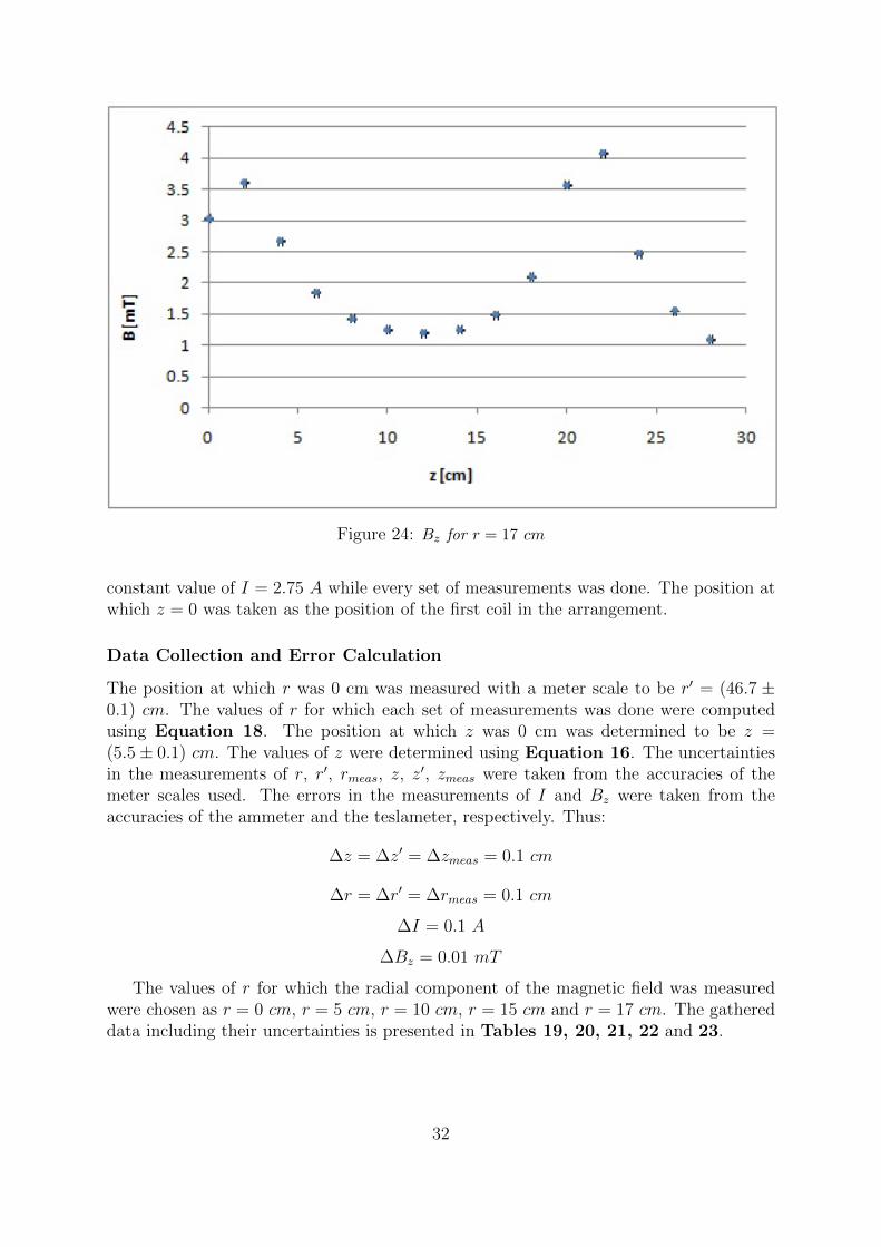
Figure 24: Bz for r = 17 cm
constant value of I = 2.75 A while every set of measurements was done. The position atwhich z = 0 was taken as the position of the first coil in the arrangement.
Data Collection and Error Calculation
The position at which r was 0 cm was measured with a meter scale to be r′ = (46.7 ±0.1) cm. The values of r for which each set of measurements was done were computedusing Equation 18. The position at which z was 0 cm was determined to be z =(5.5± 0.1) cm. The values of z were determined using Equation 16. The uncertaintiesin the measurements of r, r′, rmeas, z, z′, zmeas were taken from the accuracies of themeter scales used. The errors in the measurements of I and Bz were taken from theaccuracies of the ammeter and the teslameter, respectively. Thus:
∆z = ∆z′ = ∆zmeas = 0.1 cm
∆r = ∆r′ = ∆rmeas = 0.1 cm
∆I = 0.1 A
∆Bz = 0.01 mT
The values of r for which the radial component of the magnetic field was measuredwere chosen as r = 0 cm, r = 5 cm, r = 10 cm, r = 15 cm and r = 17 cm. The gathereddata including their uncertainties is presented in Tables 19, 20, 21, 22 and 23.
32

z′ [cm] z [cm] ∆z [cm] Br [mT ] ∆Br [mT ]5.5 0.0 0.1 -0.08 0.016.0 0.5 0.1 -0.09 0.018.0 2.5 0.1 -0.08 0.0110.0 4.5 0.1 -0.08 0.0112.0 6.5 0.1 -0.09 0.0114.0 8.5 0.1 -0.07 0.0116.0 10.5 0.1 -0.08 0.0118.0 12.5 0.1 -0.08 0.0120.0 14.5 0.1 -0.09 0.0122.0 16.5 0.1 -0.07 0.0125.0 19.5 0.1 -0.05 0.0127.0 21.5 0.1 -0.03 0.0129.0 23.5 0.1 -0.02 0.0131.0 25.5 0.1 -0.02 0.01
Table 19: Measured Br for r = 0 cm and a = R including uncertainties
z′ [cm] z [cm] ∆z [cm] Br [mT ] ∆Br [mT ]5.5 0.0 0.1 -0.11 0.016.0 0.5 0.1 -0.11 0.018.0 2.5 0.1 -0.07 0.0110.0 4.5 0.1 -0.06 0.0112.0 6.5 0.1 -0.07 0.0114.0 8.5 0.1 -0.07 0.0116.0 10.5 0.1 -0.08 0.0118.0 12.5 0.1 -0.07 0.0120.0 14.5 0.1 -0.05 0.0122.0 16.5 0.1 -0.01 0.0125.0 19.5 0.1 0.06 0.0127.0 21.5 0.1 0.12 0.0129.0 23.5 0.1 0.15 0.0131.0 25.5 0.1 0.17 0.01
Table 20: Measured Br for r = 5 cm and a = R including uncertainties
33

z′ [cm] z [cm] ∆z Br [mT ] ∆Br [mT ]5.5 0.0 0.1 -0.11 0.016.0 0.5 0.1 -0.08 0.018.0 2.5 0.1 -0.01 0.0110.0 4.5 0.1 0.01 0.0112.0 6.5 0.1 -0.03 0.0114.0 8.5 0.1 -0.09 0.0116.0 10.5 0.1 -0.14 0.0118.0 12.5 0.1 -0.17 0.0120.0 14.5 0.1 -0.13 0.0122.0 16.5 0.1 -0.02 0.0125.0 19.5 0.1 0.22 0.0127.0 21.5 0.1 0.35 0.0129.0 23.5 0.1 0.42 0.0131.0 25.5 0.1 0.43 0.01
Table 21: Measured Br for r = 10 cm and a = R including uncertainties
z′ [cm] z [cm] ∆z Br [mT ] ∆Br [mT ]5.5 0.0 0.1 0.27 0.016.0 0.5 0.1 0.38 0.018.0 2.5 0.1 0.49 0.0110.0 4.5 0.1 0.37 0.0112.0 6.5 0.1 0.12 0.0114.0 8.5 0.1 -0.11 0.0116.0 10.5 0.1 -0.34 0.0118.0 12.5 0.1 -0.60 0.0120.0 14.5 0.1 -0.74 0.0122.0 16.5 0.1 -0.50 0.0125.0 19.5 0.1 0.71 0.0127.0 21.5 0.1 1.03 0.0129.0 23.5 0.1 0.97 0.0131.0 25.5 0.1 0.82 0.01
Table 22: Measured Br for r = 15 cm and a = R including uncertainties
34

z′ [cm] z [cm] ∆z Br [mT ] ∆Br [mT ]5.5 0.0 0.1 1.06 0.016.0 0.5 0.1 1.14 0.018.0 2.5 0.1 0.93 0.0110.0 4.5 0.1 0.54 0.0112.0 6.5 0.1 0.22 0.0114.0 8.5 0.1 -0.09 0.0116.0 10.5 0.1 -0.43 0.0118.0 12.5 0.1 -0.85 0.0120.0 14.5 0.1 -1.41 0.0122.0 16.5 0.1 -1.68 0.0125.0 19.5 0.1 1.83 0.0127.0 21.5 0.1 1.72 0.0129.0 23.5 0.1 1.28 0.0131.0 25.5 0.1 0.98 0.01
Table 23: Measured Br for r = 17 cm and a = R including uncertainties
Data Evaluation
The gathered data along with the uncertainties were plotted in Figures 25, 26, 27, 28and 29.
Figure 25: Br for r = 0 cm
35

Figure 26: Br for r = 5 cm
Figure 27: Br for r = 10 cm
Discussion and Conclusion
As expected, due to symmetry, the radial component Br of the magnetic field is close to0 when the measurements are taken on the central axis of the Helmholtz arrangement.
36
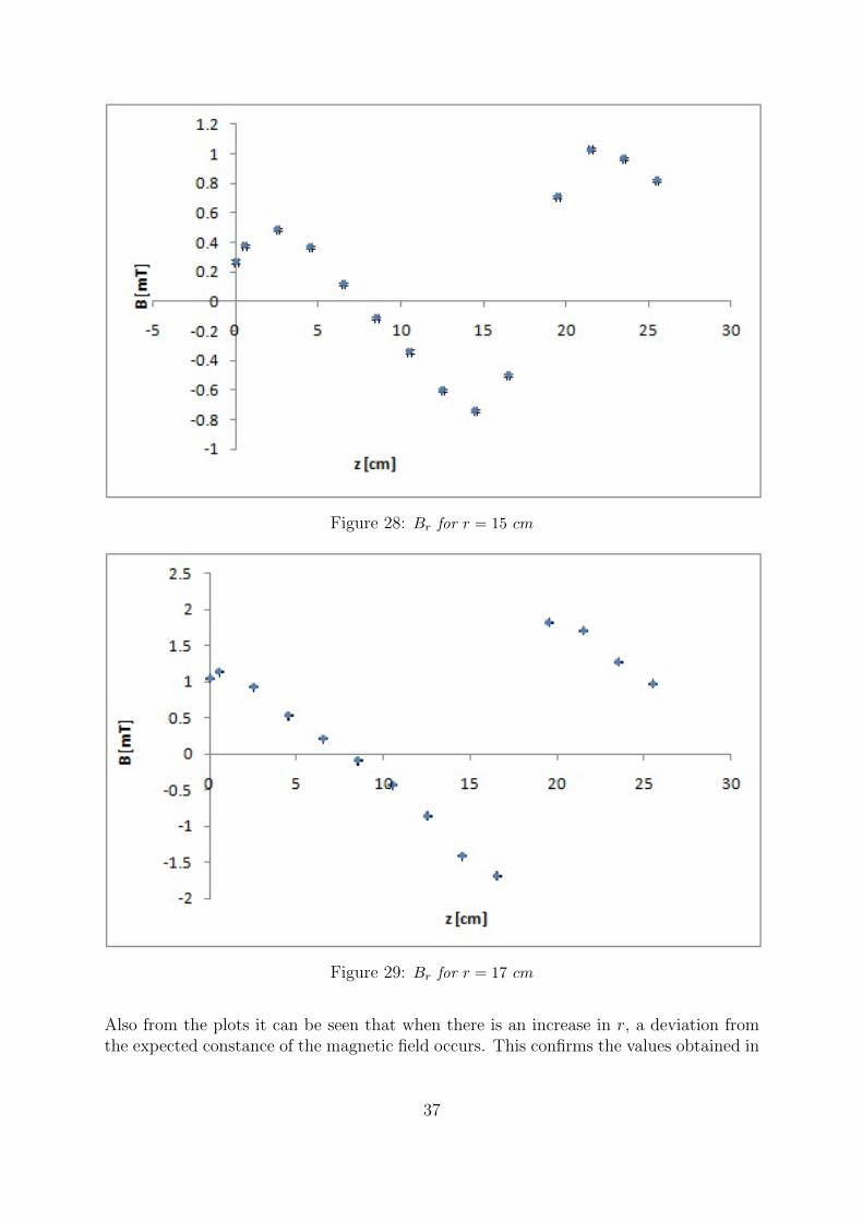
Figure 28: Br for r = 15 cm
Figure 29: Br for r = 17 cm
Also from the plots it can be seen that when there is an increase in r, a deviation fromthe expected constance of the magnetic field occurs. This confirms the values obtained in
37

the previous section. Again, a cylinder with radius r = 5 cm can be imagined inside theHelmholtz arrangement. Inside this cylinder, the magnetic field can be assumed constant.
3.3 Magnetic moment in a field of a Helmholtz coil arrangement
For the final part of the experiment, the torque experienced by a current loop in themagnetic field created by the Helmholtz coils was examined as a function of the magneticfield strength, the angle between the magnetic field and the magnetic moment and as afunction of magnetic moment. The magnetic field created by the Helmholtz coil was notdirectly measured, but, using the fact that B is directly dependent on the current flowingthrough the coils (Equation 5), the current Icoil has been analysed instead.The small conductor loop used for the experiment had n = 3 turns and the measureddiameter was:
d = (12.0± 0.1) cm
The error is given by the uncertainty of the measuring instrument. Therefore, the totalarea of the coil was computed using the formula:
A =π
4· d2 (19)
Numerically,A = 113.0 cm2
The error in the area was next computed using the averaged error formula [2]:
∆A =
√(∂A
∂d·∆d
)2
=⇒ ∆A =πd
2·∆d (20)
The obtained value was:∆A = 1.9 cm
Therefore, the total area of the conductor loop was:
A = (113.0± 1.9) cm
3.3.1 Torque as a function of the strength of the magnetic field
Data collection
For the first set of measurements, the torque as a function of the strength of the magneticfield was measured. The angle between the conductor loop from between the coils andthe magnetic field lines created by the Helmholtz coils was kept constant at 90◦:
α = 90◦
The magnetic moment of the test coil was also kept constant during the measurements.According to equation Equation 10, the magnetic moment is proportional to the currentItest passing through the conduction loop and, thus, in order to keep m constant, it wasenough to induce a constant current Itest = 1 A to the loop. In addition, as statedbefore, instead of directly measuring the magnetic field of the Helmholtz coils, the current
38

Icoil flowing through them was recorded. Moreover, from the definition of the torqueEquation 21, it is obvious that the torque is directly proportional to the force acting oneach side of the test coil.
T = r × F (21)
Consequently, in order to measure the requested dependency, the force F was measuredas a function of the current Icoil. The collected data is presented in Table 24:
α [◦] Icoil [A] Itest [A] F [mN ]90 0.51 1 0.190 0.83 1 0.290 1.04 1 0.390 1.32 1 0.390 1.72 1 0.490 2.01 1 0.590 2.3 1 0.690 2.65 1 0.790 2.96 1 0.8
Table 24: Force F as a function of the current inside the Helmholtz coils Icoil
Error calculation
The error of the measured force was chosen to be the smallest division of the dynamome-ter, determining the numerical value of:
∆F = 0.1 mN
The same procedure was applied for determining the error in the current Icoil passingthrough the Helmholtz coils, resulting in a numerical value of:
∆Icoil = 0.01 A
On the other hand, during the measurements, a variation larger than the last digit of themeasuring instrument in the current passing through the test coil was noticed. Therefore,the error in Itest was determined to be:
∆Itest = 0.05 A
In addition, the system through which the angle α was measured was quite imprecise andthus, the error ∆α was estimated to be:
∆α = 1◦
Data evaluation
Using the data gathered in Table 24, the force was plotted as a function of the currentpassing through the Helmholtz coil. The resulting plot, including the error bars, ispresented in Figure 30.
39

Figure 30: Force as a function of current passing through the Helmholtz coils (including uncer-
tainties)
Discussion and conclusion
It can be seen from Figure 30 that the force is proportional to the current in theHelmholtz coil. The coefficient of linear regression obtained using Excel c© tools assuredthat there is a dependency between the two quantities:
R2 = 0.9875
In addition, from Equation 21, the torque is proportional to the force exerted on thetest coil. Thereby, the dependence of the force on the current Icoil is equivalent to thedependence of the torque on the strength of the magnetic field. The only difference isa proportionality constant, represented here by the diameter of the conductor loop d aswell as the proportionality constant between the magnetic field and the varied current.Consequently, this difference would be reflected only on the slope of the graph. Therefore,the force increases linearly with the current passing through the Helmholtz coils.
3.3.2 Torque as a function of the angle between the magnetic field and mag-netic moment
Data collection
The same reasoning from Section 3.3.1 is applied here for the relation between torqueand force, as well as between magnetic filed and the current through the coil and magneticmoment and the current through the test coil. Moreover, for this part of the experiment,
40

both currents Icoil and Itest have been kept constant:
Icoil = 2.75 A
Itest = 3 A
The collected data is presented in Table 25
α [◦] α [rad] Icoil [A] Itest [A] F [mN ]90 1.571 2.75 3 1.675 1.309 2.75 3 1.460 1.047 2.75 3 1.445 0.785 2.75 3 1.230 0.524 2.75 3 0.715 0.262 2.75 3 0.30 0 2.75 3 0
-15 -0.262 2.75 3 -0.6-30 -0.524 2.75 3 -0.8-45 -0.785 2.75 3 -1.2-60 -1.047 2.75 3 -1.2-75 -1.309 2.75 3 -1.5-90 -1.571 2.75 3 -1.5
Table 25: Force F as a function of the angle α between the magnetic field and the magnetic
moment
In Table 25, the conversion of the value of angle α from degrees to radians have beenmade using the formula:
α [rad] = α [◦] · π180
(22)
Error calculation
The errors of the quantities presented in Table 25 are the same as those determined inSection 3.3.1. Therefore, the numerical value of the uncertainties are:∆Icoil = 0.01 A, ∆Itest = 0.05 A, ∆F = 0.1 mN and ∆α = 1◦ = 0.018 radNext, the error of sinα was computed using the averaged error formula and the result ispresented in Equation 23:
∆sinα =
√(∂sinα
∂α·∆α
)2
= ∆α · cosα (23)
Here, ∆α is expressed in radians in order to give a correct result. Also, the formula abovehas the disadvantage that the error vanishes for α = ±π
2.
Data evaluation
Using the data contained in Table 25, the dependence of the force on the angle α (inradians) between B and m has been plotted and the result in presented in Figure 31.
41

Figure 31: Force as a function of the angle α between the magnetic moment and the magnetic
field (including uncertainties)
As theoretically predicted in Equation 14, the dependence is sinusoidal. In order toobtain a more relevant result, further investigation was necessary. Thus, the force wasplotted against sinα in order to prove that the two quantities are linearly dependent.Data needed for the plot is shown in Table 26.
The resulting plot, including the error bars, is presented in Figure 32:Using Excel c© plotting tools, the coefficient of linear regression R2 was determined to
be:R2 = 0.9933
which assures that the absolute value of the force on the test coil increases linearly withincreasing the angle α between the magnetic field and magnetic moment.
Discussion and conclusion
According to Equation 14, the torque is directly proportional to sinα or, equivalently,the torque varies sinusoidally with the angle α. In addition, restating the proportionalitybetween the torque and the force F acting on the coil (Equation 21), one can see thatthe experimental results displayed in Figure 32 and 31 fulfil these prediction.Therefore, the linear relation between the force and sinα sustained by the coefficient oflinear regression from the fit in Figure 32:
R2 = 0.9933
42
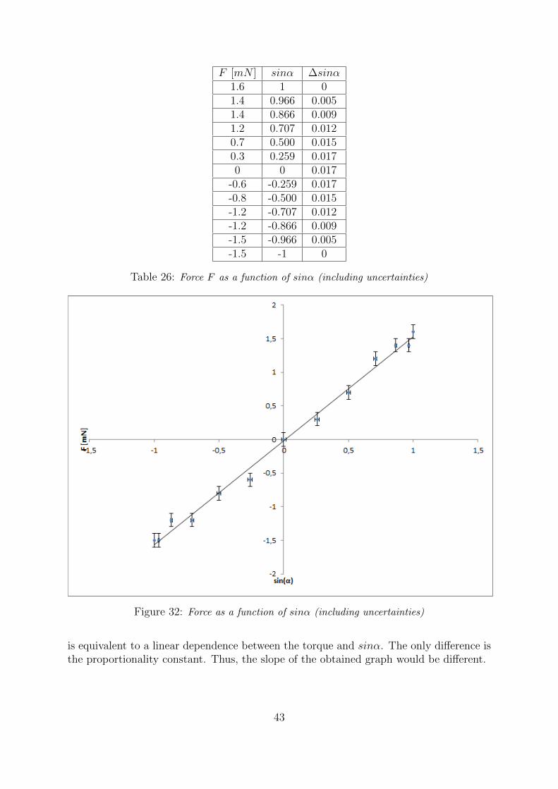
F [mN ] sinα ∆sinα1.6 1 01.4 0.966 0.0051.4 0.866 0.0091.2 0.707 0.0120.7 0.500 0.0150.3 0.259 0.0170 0 0.017
-0.6 -0.259 0.017-0.8 -0.500 0.015-1.2 -0.707 0.012-1.2 -0.866 0.009-1.5 -0.966 0.005-1.5 -1 0
Table 26: Force F as a function of sinα (including uncertainties)
Figure 32: Force as a function of sinα (including uncertainties)
is equivalent to a linear dependence between the torque and sinα. The only difference isthe proportionality constant. Thus, the slope of the obtained graph would be different.
43

3.3.3 Torque as a function of the strength of the magnetic moment
Data collection
For this part of the experiment, the torque as a function of the strength of the magneticmoment was investigated. Since the magnetic moment could not be directly measured,the same argument as in Sections 3.3.1 and 3.3.2 was followed. Hence, as the mag-netic moment is directly proportional to the current Itest in the test coil(Equation 10),the latter was recorded. Also, since the dynamometer was recording the force, the finaldiagram was the dependency of F vs Itest.Moreover, during the experiment, the magnetic field created by the Helmholtz arrange-ment was kept constant by delivering a constant current Icoil = 2.75 A to the coils andthe angle α was fixed to 90◦. The gathered data is presented in Table 27:
α [◦] Icoil [A] Itest [A] F [mN ]90 2.75 1.50 0.990 2.75 1.75 1.190 2.75 2.00 1.390 2.75 2.25 1.490 2.75 2.50 1.590 2.75 2.75 1.790 2.75 3.00 1.990 2.75 3.25 2.090 2.75 3.50 2.290 2.75 3.75 2.390 2.75 4.00 2.5
Table 27: Force F as a function of the current inside the test coil Itest
Error calculation
The errors in this section are the same as the one determined in the Sections 3.3.1 and3.3.2. Thus, the numerical values of the uncertainties are:
∆Icoil = 0.01 A, ∆Itest = 0.05 A, ∆F = 0.1 mN and ∆α = 1◦ = 0.018 rad
Data evaluation
Using the data provided in Table 27, a plot of F as a function of the current Itest wascreated and the result is presented in Figure 33:
Using Excel c© tools, the coefficient of linear regression was determined to be:
R2 = 0.9959
Discussion and conclusion
Equation 14 states that the current through a conducting coil is proportional to thetorque acting on it. Analysing Figure 33, one can see that the theoretical prediction
44

Figure 33: Force as a function of sinα (including uncertainties)
is fulfilled by the experimental results. The linear dependence is also proved by thecoefficient of linear regression
R2 = 0.9959
In addition, as stated before, the magnetic moment is proportional to the current passingthrough the test coil Itest (Equation 10) and, from definition (Equation 21), the torqueis proportional to the force acting on loop. Therefore, the analysed dependence betweenF and Itest is equivalent to the dependence between the torque and magnetic moment.The only difference is the proportionality constant which implies a different slope for theT vs m graph. Therefore, the torque increases linearly with the magnetic moment.
References
[1] Prof. Dr. Veit Wagner, Dr. Torsten Balster - Advanced Physics A+B LaboratoryCourse I, Fall 2012
[2] Prof. Dr. Jurgen Fritz, Frank Rosenkotter - Error Analysis Booklet for PhysicsTeaching Labs , 2011
Young, Freeman -University Physics, 11th Edition
45