magic plot help
TRANSCRIPT

MagicPlot 1.5 User Guide © Alexander Levantovsky, 2011
Compiled from online help on May 29MagicPlot.com
Contents
Overview.............................................................................7System Requirements and First Launch.....................................................7
Where to get the Java Virtual Machine?.......................................................7First Launch..................................................................................................7Opening Projects on Double Click................................................................7Portable Installation.....................................................................................8
Getting Started: Tables, Figures, Fit Plots and Undo...................................8Undo/Redo and History................................................................................8Where to start?............................................................................................9Creating Figures and Fit Plots......................................................................9Adding New Table to Existing Folder............................................................9Enter Expressions in any Numeric Field.....................................................10
Importing Table from Text File (ASCII).....................................................10Table Editing..........................................................................................11
Displaying Column Formulas in Table........................................................13Fit Column Widths......................................................................................13See Also.....................................................................................................13
Missing Values (NaN) in Tables and Calculations......................................13NaN in MagicPlot Tables.............................................................................14NaN in Expressions....................................................................................14
Creating a Copy of Table, Fit Plot, Folder or Figure...................................15What Data are Plotted on the Copied Fit Plots and Figures........................15
Nonlinear Curve Fitting with Fit Plot.................................16Nonlinear Curve Fitting: Fit Plot..............................................................16
Creating a Fit Plot.......................................................................................16Fitting Methodology...................................................................................16Fit Function is a Sum of Fit Curves.............................................................17Setting Initial Values of Parameters...........................................................18Guessing Peaks..........................................................................................19Parameter Locking.....................................................................................19Parameters Joining.....................................................................................19Weighting of Data Points Using Y Errors....................................................20Specifying Fit Intervals...............................................................................20Baseline Fitting and Extraction..................................................................21'Data-Baseline' Table Column....................................................................21Viewing the Residual Plot...........................................................................21Fitting.........................................................................................................22Fitting One Curve.......................................................................................22Why My Fit is Not Converged?...................................................................23See Also.....................................................................................................23
2

Fitting Algorithm and Computational Formulas.........................................24Weighting of Data Points Using Y Errors....................................................24Iterations Stop Criteria...............................................................................25Formulas....................................................................................................25See Also.....................................................................................................27
Joining the Parameters of Fit Curves........................................................27See Also.....................................................................................................29
Specifying Custom Fit Equation (Pro edition only)....................................29Fit Parameters............................................................................................30Adjusting Parameters with Mouse Wheel...................................................30See Also.....................................................................................................31
Using Spline for Baseline Subtraction (Pro edition only)...........................31Editing Spline.............................................................................................31Fitting with Spline......................................................................................32See Also.....................................................................................................33
Guessing Peaks (Pro edition only)............................................................33Smoothing of Data and 2nd Derivative......................................................34The Number of Peaks.................................................................................34See Also.....................................................................................................34
Predefined Fit Curves Equations..............................................................35See Also.....................................................................................................36
Creating x-y Table from Fit Curves...........................................................36
Data Processing................................................................37Setting Column Formula..........................................................................37
Row Index..................................................................................................37Rows Evaluation Order...............................................................................37Using Table Data........................................................................................37Auto Recalculation on Data Change...........................................................38Formula Menu in Column Context Menu....................................................38About "Argument is out of range at row #" Warning.................................39See Also.....................................................................................................39
Integration (Pro edition only)..................................................................39Baseline Correction....................................................................................40Formula......................................................................................................40See Also.....................................................................................................40
Differentiation (Pro edition only).............................................................40Formula......................................................................................................41See Also.....................................................................................................41
Fast Fourier Transform (FFT) (Pro edition only)........................................41Formulas....................................................................................................42Parameters.................................................................................................44
Histogram Calculation (Pro edition only)..................................................44Binning Options..........................................................................................44Auto Binning Criteria..................................................................................45
3

Preview Plot...............................................................................................45Descriptive Statistics (Pro edition only)...................................................46
Statistical Functions in Column Formulas..................................................46Calculating Integrals and Statistics (Pro) on Intervals using Fit Plot..........46
Managing Intervals.....................................................................................47Relative Integrals Calculation....................................................................47Formulas....................................................................................................47See Also.....................................................................................................48
Transform X or Y Fit Plot Data (Pro edition only)......................................48See Also.....................................................................................................48
Formula Syntax.......................................................................................48General Rules.............................................................................................49Functions....................................................................................................49Boolean Logic.............................................................................................50Operators...................................................................................................51
Table Sorting..........................................................................................52Sorting Criteria...........................................................................................53
Visual Data Navigation......................................................54Scale Scrolling for Data Navigation..........................................................54
Do not Confuse Scale Scrolling and Image Zoom......................................54Current Axes..............................................................................................54See Also.....................................................................................................55
Reading Plot Data, Measuring Distances, Curves Selection.......................55Crosshair Cursor.........................................................................................55Reading Plot Data......................................................................................55Curve Context Menu..................................................................................56Measuring Data Distances with Scale Zoom Tool......................................56Selecting Curves in Turn Using Keyboard..................................................57See Also.....................................................................................................58
Quick Plot Tool........................................................................................58
Editing Figures..................................................................59Adding and Arranging Axes on Figure......................................................59
Add and Arrange Axes as Table.................................................................60Adding and Arranging Curves on Figure Axes...........................................60
Changing Curves Drawing Order................................................................60Shifting Curves on Figure and Creating 2D Waterfall................................61Using Figure Templates...........................................................................63
Saving Template from Figure.....................................................................63Applying Template to a Figure...................................................................63
4

Drawing and Editing..........................................................65Axes Style Editing...................................................................................65Drawing on Figures and Fit Plots, Image Zoom and Objects Selection........65
Image Zooming (Pro edition only)..............................................................66Do not Confuse Scale Scrolling and Image Zoom......................................66Objects selection........................................................................................66Moving an Object Forward or Backward.....................................................67Changing Curves Order on Figure..............................................................67Snapping to Other Objects.........................................................................67See Also.....................................................................................................68
Colours and Opacity Adjustment..............................................................68See Also.....................................................................................................68
Creating Transparent Figures and Fit Plots..............................................68See Also.....................................................................................................69
Using of Drawing Dimensions Toolbar......................................................69Switching Curves Antialiasing on the Screen............................................70
Text Labels Editing............................................................71Inserting Special Symbols and Greek Letters............................................71
Typing Greek letters with Keyboard Shortcuts...........................................71Inserting Math Symbols with Keyboard Shortcuts......................................71Inserting Special Characters by Character Sequences...............................72Unicode Code Point Finding out.................................................................72See Also.....................................................................................................73
Advanced Typography Features...............................................................73Ligatures Support.......................................................................................73Mathematical Symbols in Axes Labels.......................................................74See Also.....................................................................................................74
Image Exporting and Copying...........................................75Image Export..........................................................................................75
Raster Image Formats................................................................................75Vector Image Formats (Pro edition only)....................................................76See Also.....................................................................................................76
Preview Image........................................................................................76Preview Features........................................................................................76Preview Zoom Options...............................................................................77
Copying Images to Clipboard (Pro edition only)........................................77See Also.....................................................................................................77
Tools..................................................................................78MagicPlot Calculator...............................................................................78
Using the Calculator...................................................................................78Standalone Calculator Application.............................................................78
5

See Also.....................................................................................................79
Appendices........................................................................80Portable Installation on USB drive...........................................................80MagicPlot Editions Comparison................................................................80Keyboard Shortcuts................................................................................82
Common Shortcuts.....................................................................................83Table Shortcuts..........................................................................................83Figure and Fit Plot Shortcuts......................................................................83
6
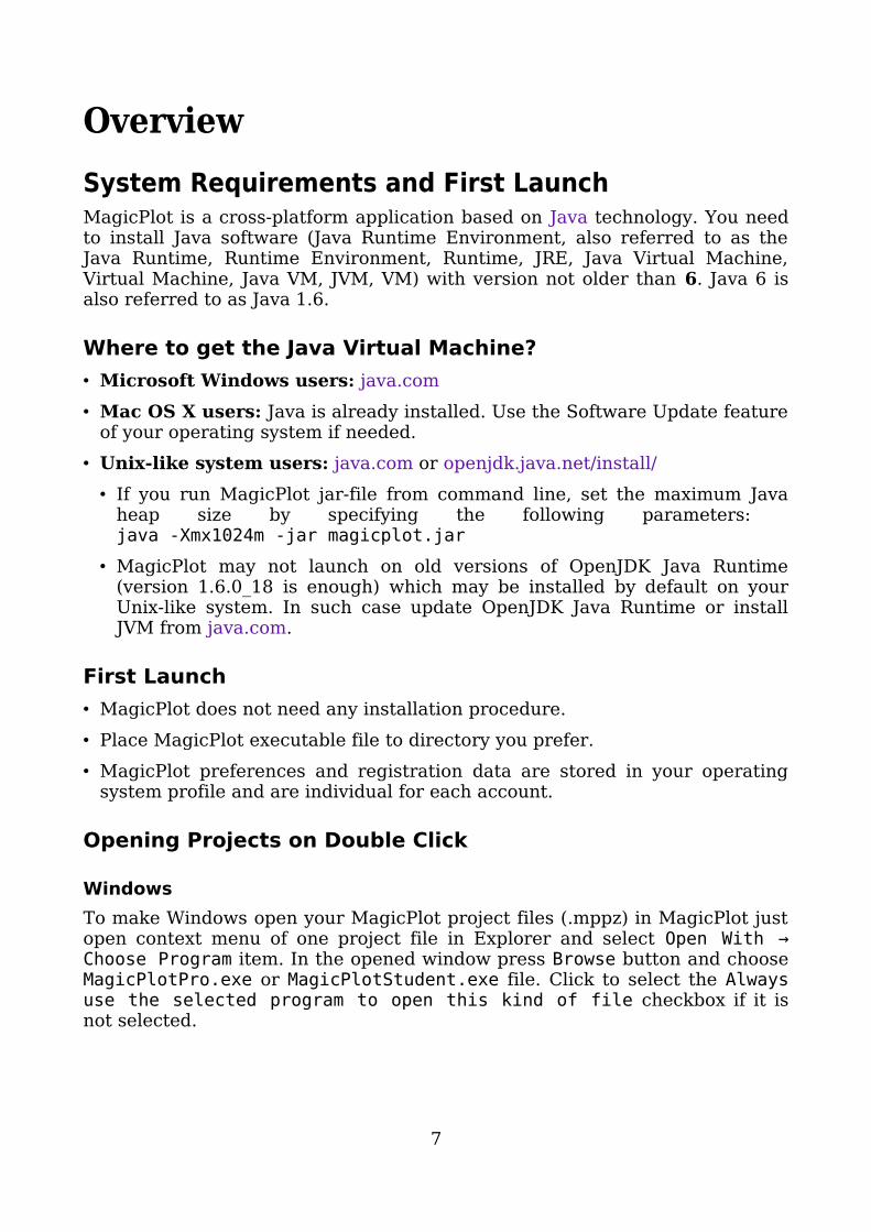
OverviewSystem Requirements and First LaunchMagicPlot is a cross-platform application based on Java technology. You need to install Java software (Java Runtime Environment, also referred to as the Java Runtime, Runtime Environment, Runtime, JRE, Java Virtual Machine, Virtual Machine, Java VM, JVM, VM) with version not older than 6. Java 6 is also referred to as Java 1.6.
Where to get the Java Virtual Machine?• Microsoft Windows users: java.com• Mac OS X users: Java is already installed. Use the Software Update feature
of your operating system if needed.• Unix-like system users: java.com or openjdk.java.net/install/
• If you run MagicPlot jar-file from command line, set the maximum Java heap size by specifying the following parameters: java -Xmx1024m -jar magicplot.jar
• MagicPlot may not launch on old versions of OpenJDK Java Runtime (version 1.6.0_18 is enough) which may be installed by default on your Unix-like system. In such case update OpenJDK Java Runtime or install JVM from java.com.
First Launch• MagicPlot does not need any installation procedure.• Place MagicPlot executable file to directory you prefer.• MagicPlot preferences and registration data are stored in your operating
system profile and are individual for each account.
Opening Projects on Double Click
WindowsTo make Windows open your MagicPlot project files (.mppz) in MagicPlot just open context menu of one project file in Explorer and select Open With → Choose Program item. In the opened window press Browse button and choose MagicPlotPro.exe or MagicPlotStudent.exe file. Click to select the Always use the selected program to open this kind of file checkbox if it is not selected.
7

Mac OS XMagicPlot project files (.mppz) will be automatically associated with MagicPlot by your operating system.
Portable InstallationMagicPlot can be installed on USB-drive. See Portable Installation on USB drive for details.
Getting Started: Tables, Figures, Fit Plots and UndoMagicPlot Projects contain Tables, Figures and Fit Plots. MagicPlot Project files have .mppz extension.• Tables contain only numerical data. • Tables which contain associated data are located in one Folder.• Fit Plots are intended for non-linear curve fitting and subtracting baselines.• Figures are intended to graphically represent multiple data.
Project treeTypically, you need to open, edit, process, plot and fit multiple data acquired in various experiments or series of experiments within single project. Ordinarily you have the source (imported) Table and a number of Tables with derivative data, such as Fourier transform or statistics of source Table data. MagicPlot automatically creates a new Folder every time you import new Table. All derivative data is stored in the same Folder by default. All Plots created from Tables in certain Folder are stored in the same Folder.
Close Unused Internal WindowsFeel free to close currently unused interval windows with Tables, Figures and Fit Plots. The data will not be deleted, the window will be closed only. You can open the closed window by double clicking on component in Project tree.
Undo/Redo and HistoryMagicPlot supports unlimited depth undo/redo function with History dialog
8

window. History dialog supports multiple undo and redo. Undone actions are marked light gray. Last saved state is set off in bold.
Undo/Redo and History menu History dialog
Where to start?In most cases you may start with importing table from text file by clicking Project → Import Text Table menu item.
Creating Figures and Fit PlotsThe easiest way to create Figure or Fit Plot is the following:• Select two columns (x and y) in Table containing your data• Select Create Figure or Create Fit Plot item in the Table context menuYou may also use Create Figure or Create Fit Plot buttons in the toolbar.
Adding New Table to Existing FolderYou can add new table to existing folder by selecting New Table in Folder context menu.
Folder context menu
9

Enter Expressions in any Numeric FieldMagicPlot can evaluate simple expressions entered in any numeric text field (brackets are supported, see formula syntax for details.) For example, you can enter 12/pi in circle width and height fields in Dimensions toolbar if you want its perimeter to be equal to 12 (remember that p=πd, where p is perimeter and d is diameter):
All numeric fields support expressions
Importing Table from Text File (ASCII)Use Project → Import Text Table menu item to import table(s) from text file(s), also referred to as ASCII file(s).You may select multiple files in opened standard file dialog by holding Ctrl or Shift.• If you open multiple files, you can select the file to preview in files drop-
down list (in Text Input Preview frame)• If you select incorrect file(s) by mistake, click on Open icon to open file
dialog once again and select other file(s).• You can set Create Figure or Create Fit Plot checkbox to create Figure
of Fit Plot after importing:• If you select Figure, the created Figure will contain all imported data from
all files• If you select Fit Plot, one Fit Plot will be created for each imported file
• You can enlarge a part of the preview plot by selecting an area by mouse (scale box zoom tool). Use context menu of the plot to change scale zoom to default.
• F5 key reloads the text file or reloads the data from clipboard.
10
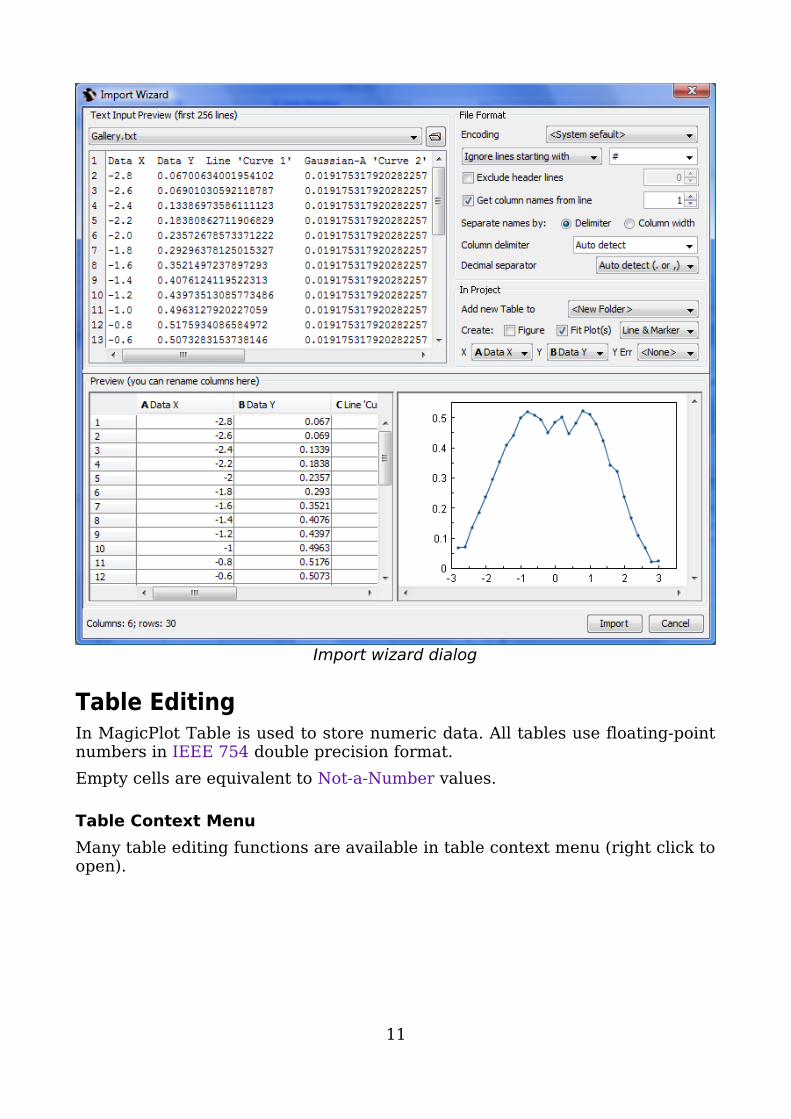
Import wizard dialog
Table EditingIn MagicPlot Table is used to store numeric data. All tables use floating-point numbers in IEEE 754 double precision format.Empty cells are equivalent to Not-a-Number values.
Table Context MenuMany table editing functions are available in table context menu (right click to open).
11

Table context menu
Columns NumbersColumns are enumerated starting with 1. The first 26 columns are additionally denoted with Latin letters: A, B, C, … Y, Z, 27, 28, 29, …. You can use either numbers or letters, addressing cells and columns in formulas.
Renaming ColumnsDouble click on column header to rename table column. You can also use Rename Column context menu item or press F4.
Moving (Reordering) ColumnsHold Alt key (Option on Mac, Meta/Win on Unix-like) and drag column header to rearrange table columns. If Alt key is not pressed, mouse dragging on header will select the columns.
Editing TableYou can edit table cell by double clicking on it. You can enter either a number or an expression (e.g. typing pi in a cell results in 3.1416…, typing 1+2 results in 3). See Formula Syntax section for expression syntax.
12

Displaying Column Formulas in TableMagicPlot marks columns for which formulas or other evaluators (FFT, integral, etc.) are set with blue header color. You can see the formula in column header tool tip.The columns which are auto recalculated are not editable and have green background instead of white.
Table header highlightingOn the screenshot above:• Column A has no formula• Column B has a formula, auto recalculation is off• Column C has a formula, auto recalculation is on, so this column is not
editable
Fit Column WidthsTo fit the width of one column, double click on right separator line in table header. To fit several selected columns widths, double click on one of column separators in table header.
See Also• Setting Column Formula• Formula Syntax• Table Sorting• Missing Values (NaN) in Tables and Calculations
Missing Values (NaN) in Tables and CalculationsIn computing, NaN, which stands for Not a Number, is a value or symbol that is usually produced as a result of an operation on invalid input operands. For example, most floating-point units are unable to explicitly calculate the square root of negative numbers, and will instead indicate that the operation was invalid and return a NaN result.An invalid operation is not the same as an arithmetic overflow (which returns
13

a positive or negative infinity). Arithmetic operations involving NaN always produce NaN, allowing the value to propagate through a calculation so that errors can be detected at the end without extensive testing during intermediate stages. A NaN does not compare equal to any number or NaN.
How does a NaN appear?There are three kinds of operations which return NaN:1. Operations with a NaN as at least one operand, e.g. 1+NaN2. Indeterminate forms
• Divisions 0/0, ∞/∞, ∞/-∞, -∞/∞, -∞/-∞• Multiplications 0*∞, 0*(-∞)• Power 1^∞• Additions ∞+(-∞), (-∞)+∞ and equivalent subtractions.
3. Real operations with complex results• Square root of a negative number• Logarithm of a negative number• Tangent of an odd multiple of 90 degrees (or π/2 radians)• Inverse sine or cosine of a number which is less than -1 or greater than
+1.
ExamplesExpression Result
0^0 1 0/0 NaN sqrt(-1) NaN 1/0 Infinity -1/0 -Infinity
NaN in MagicPlot TablesIn MagicPlot NaN is also used to represent empty cells in Tables.Statistical functions ignore NaN values in Tables.
NaN in ExpressionsYou can use predefined constants NaN, nan or NAN in expressions to specify NaN value.
Example
• If you set a Column Formula if(col(B) >= 0, col(B), NaN), it will return only positive values from column B. Negative values are replaced with NaN value. You can use this expression to filter negative values if you do not
14
want to use them in future calculations. Note that ”Not-a-Number returned at row #” warning can be shown for such expressions.
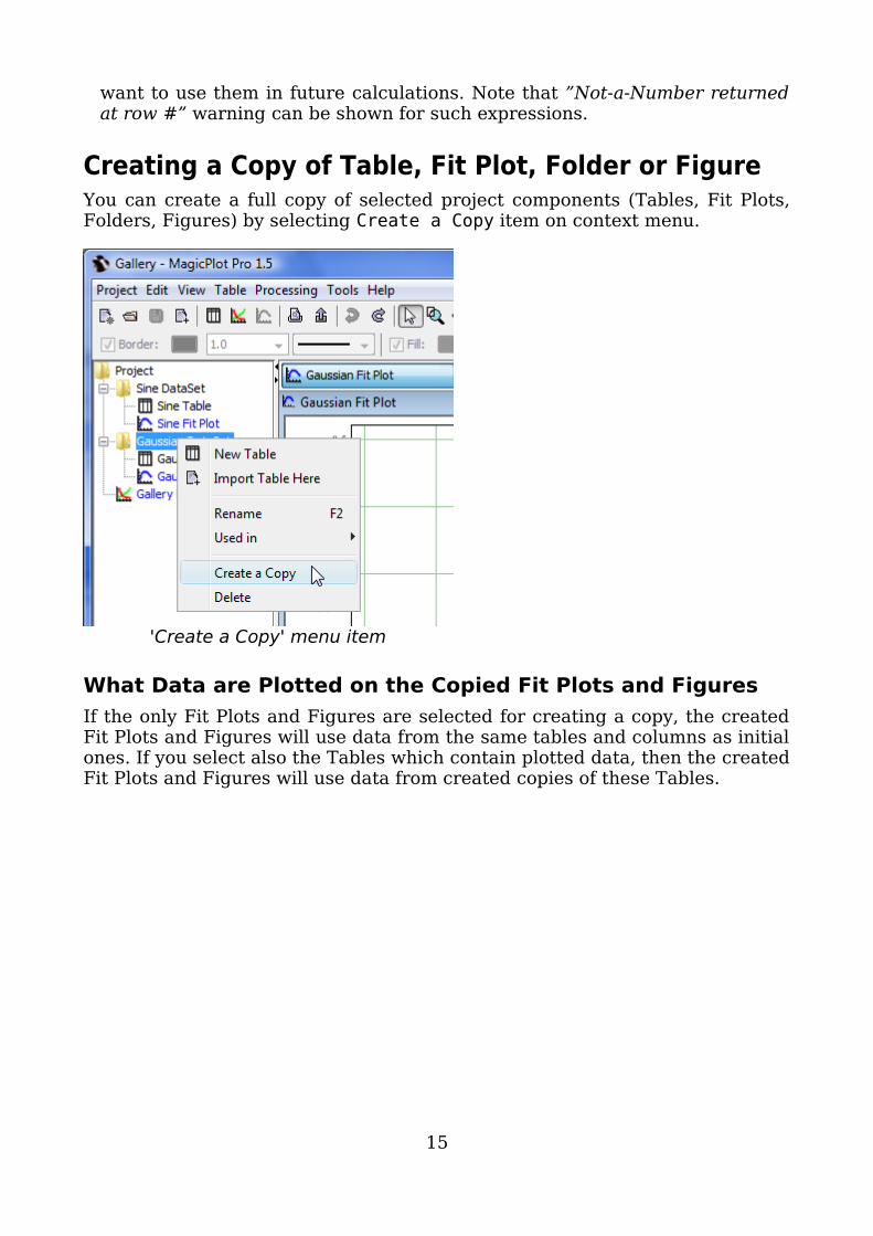
Creating a Copy of Table, Fit Plot, Folder or FigureYou can create a full copy of selected project components (Tables, Fit Plots, Folders, Figures) by selecting Create a Copy item on context menu.
'Create a Copy' menu item
What Data are Plotted on the Copied Fit Plots and FiguresIf the only Fit Plots and Figures are selected for creating a copy, the created Fit Plots and Figures will use data from the same tables and columns as initial ones. If you select also the Tables which contain plotted data, then the created Fit Plots and Figures will use data from created copies of these Tables.
15
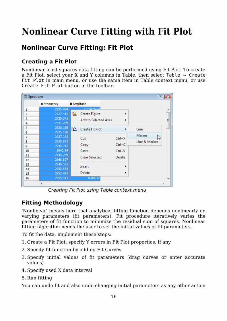
Nonlinear Curve Fitting with Fit PlotNonlinear Curve Fitting: Fit PlotCreating a Fit PlotNonlinear least squares data fitting can be performed using Fit Plot. To create a Fit Plot, select your X and Y columns in Table, then select Table → Create Fit Plot in main menu, or use the same item in Table context menu, or use Create Fit Plot button in the toolbar.
Creating Fit Plot using Table context menu
Fitting Methodology'Nonlinear' means here that analytical fitting function depends nonlinearly on varying parameters (fit parameters). Fit procedure iteratively varies the parameters of fit function to minimize the residual sum of squares. Nonlinear fitting algorithm needs the user to set the initial values of fit parameters.To fit the data, implement these steps:1. Create a Fit Plot, specify Y errors in Fit Plot properties, if any2. Specify fit function by adding Fit Curves3. Specify initial values of fit parameters (drag curves or enter accurate
values)4. Specify used X data interval5. Run fittingYou can undo fit and also undo changing initial parameters as any other action
16

using Undo function. It is a handy feature when experimenting with different models and initial parameters.
Further readingThis manual does not completely cover the complex nonlinear fitting methodology. We recommend you to take a look at this book:• H. Motulsky and A. Christopoulos, Fitting Models to Biological Data Using
Linear and Nonlinear Regression: A Practical Guide to Curve Fitting. 2003, GraphPad Software Inc., San Diego CA, graphpad.com. PDF is available for free here.
Fit example
Fit Function is a Sum of Fit CurvesMagicPlot considers fit function as a sum of Fit Curves. Ordinarily in peaks fitting each Fit Curve corresponds to one peak in experimental data. Click the Add button to add new Fit Curve to the list. There is a number of predefined Fit Curves types (Line, Parabola, Gauss, Lorentz, etc.) You can also create a Custom Equation Fit Curve and manually enter the formula (Pro edition only). Baseline fitting components may be added to the fitting sum, too.Fit Plot window contains the list of Fit Curves. Each Fit Curve in the list has three checkboxes:
17

Fit Curves table• Show: Specifies whether to show this Fit Curve on plot. Active only if
Baseline checkbox is not set• Baseline: Toggles the subtracting of this Fit Curve from experimental data.
You also can use Residual button to subtract all Fit Sum from data• Sum: Specifies whether to use this Fit Curve in sum fit functionBelow the Fit Curves list is a parameters table which shows names, values, and descriptions of parameters relating to selected Fit Curve.
Fitting by Sum and Fitting One CurveMagicPlot allows two alternatives buttons to run the fit:• Fit by Sum button will fit the data with the sum of Fit Curves for which the Sum checkbox is set. Data interval from Fit Interval tab will be used. This button must be used for example to fit the spectrum with the sum of peaks.
• Fit One Curve button will fit the data with the one currently selected Fit Curve. Individual interval for each Fit Curve will be used. Set Edit Interval checkbox to edit individual interval for each Fit Curve.
Copying and Pasting Fit CurvesYou can copy and paste Fit Curves from one Fit Plot to another Fit Plot or Figure. You can also paste the copied Fit Curves to the same Fit Plot to create a copy.• The copy of Fit Curves with the same parameters and styles will be created
if you paste Fit Curves to a Fit Plot.• A link to the source Fit Curves will be inserted if you paste Fit Curves in a
Figure.
Fit Curves ReorderingYou can reorder Fit Curves by dragging them in table. The data curve is always drawn the first and fit sum is drawn the last.
Setting Initial Values of ParametersNonlinear fitting assumes that certain initial values of parameters are set before fitting. This procedure is very easy if you use Fit Curves of predefined
18

types (not custom equation): you can drag curves on plot. Initial parameters values for each Fit Curve can also be set in parameter table.
Moving curves with mouse
Adjusting Parameters with Mouse WheelYou can adjust Parameters in table using mouse wheel scrolling when mouse cursor is on the desired parameter: Hold Ctrl key (Cmd key on Mac) and scroll. If Shift key is also pressed the parameter step for one wheel 'click' will be increased.
Guessing PeaksIf you are fitting a spectrum with multiple peaks, MagicPlot may automatically add and approximately locate peaks before fitting (Pro edition only). See Guessing Peaks (Pro edition only) for details. Guessed peaks should be used only as the initial estimate for fitting.
Parameter LockingYou can lock (fix) parameter(s) to prevent varying this parameter(s) during fit and to prevent its changing due to setting initial values by mouse dragging (for built-in functions). Set the checkbox in Lock column in parameters list to lock parameter.
Table of Parameters
Parameters JoiningMagicPlot allows joining (sometimes referred to as coupling, binding, linking) of fit parameters of different Fit Curves. See Joining the Parameters of Fit Curves for details.
19

Weighting of Data Points Using Y ErrorsMagicPlot allows data points weighting with Y error data. You can specify Y error data in Fit Plot properties dialog. If no Y error data are specified weighting is not used.
Weights are calculated as 1 / Yerror2 for every point. See Fitting Algorithm
and Computational Formulas for details.Weights must be positive and finite for all points so the Y error values must be positive and non-zero (to prevent infinite weights). MagicPlot checks this condition before fitting and shows an error message if Y errors cannot be used to compute weights.
Specifying Fit IntervalsYou can set the X intervals of the data which will be used for fitting. Data points outside these intervals are not used to compute the minimizing residual sum of squares. You can use this feature if some data points (especially in the beginning or the end) are inaccurate, e.g. noisy.Select Fit Interval tab to set intervals visually or edit accurate borders values in table.• Double click on interval to split it• Drag the interval border to move it. If intervals intersect, they will be
merged• Use context menu on the plot to create, delete and split intervalsNote: Data intervals from Fit Interval tab are used for fitting Sum only. To set individual data intervals for the one Curve fitting use Edit Interval checkbox.
20

Fit interval context menu
Baseline Fitting and ExtractionFit Interval is also usable when baseline fitting. Before baseline fitting you can specify the interval which does not contain any signal points and contains baseline only. Set Baseline checkboxes at baseline Fit Curves after baseline fitting to subtract baseline from data. Then specify the whole interval and fit the data.Note that if you use data processing (integration, FFT, etc.) on Fit Plot, then the difference between the data and baseline curves (which you do see on the plot) will be processed. You can use this behaviour to exclude baseline from data before integrating, see Integration (Pro edition only) for more information.
'Data-Baseline' Table ColumnThe 'Data-Baseline' column is appended to the Table with initial (X and Y) data when you create a Fit Plot. The 'Data-Baseline' column contains the difference between initial Y data and baseline approximation (the sum of Fit Curves for which Baseline checkbox is set). It is 'Data-Baseline' column that is actually plotted on Fit Plot as data.Use 'Data-Baseline' column in Table if you want to process the data without baseline. This column is also used as initial data if you use Processing menu when Fit Plot is active.
Viewing the Residual PlotResidual means here the difference between initial data, baseline function and Fit Sum function. MagicPlot offers two different ways to view the residual:
21

• Press and hold the Residual button. The residual will be shown while button is pressed. You can use either mouse or space key (if button is selected) to hold Residual button.
• You can either set Baseline checkboxes for all summed Fit Curves to subtract them from data and explore the residual plot
FittingTo execute the fit click the Fit by Sum button of Fit One Curve button (see below).MagicPlot indicates fit process with a special window. Fitting curves are periodically updated on plot while fitting so you can see how fit converges.
Fit progress windowMagicPlot shows current iteration number and deviation decrement with two progress bars while fit is performed. The fit process stops when one of these progress bars reaches the end.You can see two buttons on fit progress window:• Break Iterations: Breaks iterations after current iteration. Use this button
if you suspect that further iterations will not change the result.• Undo Fit: Breaks iterations and reverts fit parameters to their initial (before
fit) values. Use this button if you see that fit process converges to wrong result; change initial values of parameters and run fit again.
Fitting One CurveYou can use MagicPlot to fit the data with single selected Fit Curve by pressing Fit One Curve button. In this case a specific data interval for each Fit Curve is used and the main fitting data interval (from Fit Interval tab) is ignored. Select Edit Interval checkbox in the bottom of the Fit Plot panel to set specific fit intervals for each Fit Curve.Because of using individual data interval this method is useful for baseline fitting. In order to fit baseline specify the intervals which does not contain signal (peaks) and contain only noise.
22

'Fit One Curve' button
Why My Fit is Not Converged?In some cases the fit procedure may fail to find the optimal parameters values. The actual mathematical reason for this error is impossibility to invert the matrix α calculated from partial derivatives of fit function with respect to fit parameters. This inverted matrix is used to compute the new values of parameters for next step of fit (like gradient descent). In most cases this error occurs when the matrix α is ill-conditioned or nearly singular and the inverse cannot be calculated accurately enough with used floating-point arithmetic.
The origin of this error may be:
• Fit is not converged through one or more parameters: some parameters were taking unrealistically great values during iterations. There are no local minimum of residual sum of squares near the initial values of these parameters. MagicPlot highlights the suspicious Fit Curve in this case.
• Mutual dependency exists between some parameters. The algorithm cannot resolve which parameter to vary.
• Fit function is ill-conditioned: the minimized residual sum of squares depends on some parameters much more than on other ones.
Try one of the following:
• Specify more accurate initial values of parameters.• Simplify the fit function (e.g. remove some peaks).• Lock some parameters.
See Also• Fitting Algorithm and Computational Formulas• Specifying Custom Fit Equation (Pro edition only)• Using Spline for Baseline Subtraction (Pro edition only)• Joining the Parameters of Fit Curves• Guessing Peaks (Pro edition only)• Predefined Fit Curves Equations
23

• Transform X or Y Fit Plot Data (Pro edition only)• Calculating Integrals and Statistics (Pro) on Intervals using Fit Plot• Creating x-y Table from Fit Curves
Fitting Algorithm and Computational FormulasMagicPlot uses iterative Levenberg–Marquardt nonlinear least squares curve fitting algorithm which is widely used in most software.Fit procedure iteratively varies the parameters βk of fit function f(x, β1, …, βp) to minimize the residual sum of squares (RSS, χ2):
here:• xi and yi are the data points,
• N is total number of points,• f(x, β1,…,βp) is the fit function which depends on value of x and fit
parameters βk,
• p is the number of fit parameters βk,
• wi are normalized (Σwi = 1) data weighting coefficients for each point (xi, yi).
An initial guess for the parameters has to be provided to start minimization. Calculation of the new guess of parameters on each fit iteration is based on the fit function partial derivatives for current values of fit parameters and for each x value:
Weighting of Data Points Using Y ErrorsMagicPlot can use weighting of y values based on y errors si:
• If standard y errors are not specified: all wi=1
• If standard y errors si are specified:
here C is normalizing coefficient (to make the sum of wi be equal to N):
24

In Fit Plot Properties dialog (Plot Data tab) you can set one of the following methods to evaluate standard y errors si:
• Get y errors from table column(s),• Percent of data for every point,• Fixed value or Standard deviation — do not use in weighting because in this
case the error values are the same for all data points.
Iterations Stop CriteriaAfter each iteration except the first MagicPlot evaluates deviation decrement D:
Deviation decrement shows how the residual sum of squares (RSS) on current iteration relatively differs from that on the previous iteration.The iterative fit procedure stops on one of two conditions:• If the deviation decrements D for two last iterations is less than minimum
allowable deviation decrement, which is 10-9 by default• If the number of iterations exceeds maximum number of iterations, which is
100 by defaultYou can change the minimum allowable deviation decrement and maximum number of iterations in Fitting tab of MagicPlot Preferences.
FormulasIn the table below you can find the formulas which MagicPlot uses to calculate fit parameters and values in Fit Report tab.Because of some confusion in the names of the parameters in different sources (books and software), we also give many different names of same parameter in note column.
Parameter Name
Symbol Formula Note
Original Data and Fit Model Properties Number of used data points
— This is the number of data points inside specified Fit Interval.
Fit parameters β1,…,βp — For peak-like functions (Gauss, Lorentz) these parameters are amplitude, position and half width at half maximum.
25

Number of fit function parameters β
— This is the total number of parameters of all fit curves which are summarized to fit.
Degrees of freedom
Estimated mean of data
Estimated variance of data
Not used by fit algorithm, only for comparison.
Data total sum of squares, TSS
TSS
TSS is also called sum of squares about the mean and acronym SST is also used.
Fit Result Residual sum of squares, RSS
This value is minimized during the fit to find the optimal fit function parameters. RSS is also called the sum of squared residuals (SSR), the error sum of squares (ESS), the sum of squares due to error (SSE).
Reduced χ2
The advantage of the reduced chi-squared is that it already normalizes for the number of data points and model (fit function) complexity. Reduced χ2 is also called mean square error (MSE) or the residual mean square.
Residual standard deviation
s
Standard deviation is also called root mean square of the error (Root MSE)
Coefficient of determination
R2 will be equal to one if fit is perfect, and to zero otherwise. This is a biased estimate of the population R2, and will never decrease if additional fit parameters (fit curves) are added, even if they are irrelevant.
Adjusted R2 Adjusted R2 (or degrees of freedom adjusted R-square) is a slightly modified version of R2, designed to penalize for the excess number of fit parameters (fit curves) which do not add to the explanatory power of the regression. This statistic is always smaller than R2, can decrease as you add new fit curves, and even be negative for poorly fitting models
Covariance matrix of parameters βk
Here α is the matrix of partial derivatives of fit function with respect to parameters βm and βn which is used for fitting:
26

Standard deviation of parameters βk,std. dev.
Correlation matrix of parameters βk
See Also• Nonlinear Curve Fitting: Fit Plot• Specifying Custom Fit Equation (Pro edition only)• Using Spline for Baseline Subtraction (Pro edition only)• Joining the Parameters of Fit Curves• Guessing Peaks (Pro edition only)• Predefined Fit Curves Equations• Transform X or Y Fit Plot Data (Pro edition only)• Calculating Integrals and Statistics (Pro) on Intervals using Fit Plot
Joining the Parameters of Fit CurvesIn some cases you may want to fit the data with two peaks with the same amplitude for example. You can do this in two ways: by specifying custom Fit Curve with your equation or by joining the 'amplitude' parameters of two peaks.
27

Joining parameters exampleTo join parameters of two or more Fit Curves select one of desired Fit Curves, then select desired parameter in parameters table and press Join button in the bottom of the panel (or double click on parameter). You can specify the selected parameters as equal or proportional by entering multiplier and constant for each parameter. Joined parameters are shown with blue color (instead of black) in curve parameters table in Fit Plot window. Joined parameters are treated as one parameter when fitting, so joining results in the reducing of actual model parameters number.In the example above the areas and widths of tho peaks are joined and are equal. The positions of maximums are joined and inverse: -1 multiplier is set to the width of Curve 3.
Joining the areas of two peaks
28

Joining the positions of two peaks
See Also• Nonlinear Curve Fitting: Fit Plot
Specifying Custom Fit Equation (Pro edition only)To specify custom fit function formula, press Add button and select Custom Equation in popup menu.• Enter your formula in y(x)= text field below. Use x as fit function argument.
See formula syntax for details.• You may recall last entered custom fit functions using Recently Used Custom item in Add popup menu.
29

Custom fit function example
Fit ParametersYou can introduce Fit Curve parameters with any names except argument x, and constants like e, pi (see predefined constants for details):• Parameters names are case-sensitive (a and A are different parameters).• Parameters names lengths are not limited.• Begin names with letter or _ sign. You can use numbers in the middle or in
the end of the name: a1, a_1, A1, a1t, but the names like 1a are not allowed.
The parameters you introduce in formula will automatically and immediately occur in parameters list, you do not need to enter parameters names in the list manually. Random values are used as the initial values of parameters. Do not forget to set more relevant initial values, otherwise fit algorithm may fail.
Adjusting Parameters with Mouse WheelYou can adjust Parameters in table using mouse wheel scrolling when mouse cursor is on the desired parameter: Hold Ctrl key (Cmd key on Mac) and scroll. If Shift key is also pressed the parameter step for one wheel 'click' will be increased.
30

See Also• Nonlinear Curve Fitting: Fit Plot• Using Spline for Baseline Subtraction (Pro edition only)• Predefined Fit Curves Equations
Using Spline for Baseline Subtraction (Pro edition only)You can use cubic spline to subtract baseline on Fit Plot. To create spline curve click on Add button in Fit Curves tab of Fit Plot and select Spline menu item. Do not use splines to subtract baselines which can be fit well enough with Line curve (line or constant baseline). You may mistakenly subtract wide peaks using spline. In some cases Parabola curve may be more suitable.
Editing SplineCreated spline has three anchor points by default. You can move, add and remove anchor points:• Move anchor point with mouse• Double click on spline curve to add new anchor point• Double click on anchor point to remove itSet Baseline checkbox in spline row in fit curves table to subtract spline from data.
Using spline for baseline fitting
31

Fitting with SplineSpline anchor point (x, y) coordinates are treated as fit parameters so you can perform fitting with spline although we don't recommend this technique. Fitting the baseline with some adequate model function is preferred. It is recommended to set appropriate fit intervals which contain only baseline without peaks. In such case Fit One Curve button is more acceptable than Fit by Sum button, because the individual interval for current curve will be used and the interval from Fit Interval tab (which is used to fit by sum of curves) is ignored. Select spline curve and set Edit Interval checkbox in the bottom of the panel to edit spline interval, then click on Fit One Curve button. The anchor point coordinates will be varied but the number of points will remain. You also can lock some parameters (usually x coordinates) by setting Lock checkboxes in parameters table.
Setting Fit Interval for spline curve
32

Spline subtraction result
See Also• Nonlinear Curve Fitting: Fit Plot• Specifying Custom Fit Equation (Pro edition only)• Guessing Peaks (Pro edition only)• Predefined Fit Curves Equations
Guessing Peaks (Pro edition only)MagicPlot can approximately locate peaks in spectrum. To locate peaks click on Guess button in Fit Curves tab of Fit Plot. Peak guessing is performed by looking for local minimums of second derivative of data-baseline.When Guess Peaks window is open you can see the preview of guessed peaks on Fit Plot. This preview is updated every time you change the parameters in the window.
33

Guess peaks dialog
Smoothing of Data and 2nd DerivativeSmoothing is used in order to filter narrow peaks which can be guessed from noise. MagicPlot peak guess tool is capable of smoothing both data and second derivative before finding local minimums. Smoothing is used only to find peaks and does not affect the data on Fit Plot.Savitzky–Golay method is used for smoothing. This algorithm performs a local polynomial regression of specified degree on specified number of points. The more points, the smoother is curve.
The Number of PeaksMagicPlot sorts found peaks by amplitude and suggests only a specified number of greatest peaks. You can change the number of guessed peaks with slider or by entering value in the text field with spinner.
See Also• Nonlinear Curve Fitting: Fit Plot• Specifying Custom Fit Equation (Pro edition only)• Using Spline for Baseline Subtraction (Pro edition only)
34

• Predefined Fit Curves Equations
Predefined Fit Curves EquationsAll predefined Fit Curves are listed in this table. You also can specify custom fit equation. Unlike custom fit equations these curves can be adjusted with mouse on Fit Plot.
Name Formula Additional Properties Line Parabola Vertex:
Gaussian
Area:
Standard deviation:
Gaussian-A (normalized)
Amplitude:
Standard deviation:
Lorentzian
Area:
Lorentzian-A (normalized)
Amplitude:
Gauss Derivative
Area (second integral):
Standard deviation:
Peak-to-peak horizontal:
Peak-to-peak vertical:
Lorentz Derivative
Area (second integral):
Peak-to-peak horizontal:
35

Peak-to-peak vertical:
See Also• Nonlinear Curve Fitting: Fit Plot• Using Spline for Baseline Subtraction (Pro edition only)• Guessing Peaks (Pro edition only)
Creating x-y Table from Fit CurvesFit Curves and Fit Sum are treated as function equations in MagicPlot Fit Plots. But in some cases (e. g. to export and plot fit data with other application) you may want to create (x, y) table with Fit Curves y-values. For this purpose use Project → Create Table from Curves menu item when Fit Plot is active.You can either add new Table to a Folder in current Project or export table to a text file.
Create Table from Curves window
36
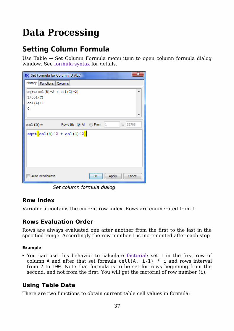
Data ProcessingSetting Column FormulaUse Table → Set Column Formula menu item to open column formula dialog window. See formula syntax for details.
Set column formula dialog
Row IndexVariable i contains the current row index. Rows are enumerated from 1.
Rows Evaluation OrderRows are always evaluated one after another from the first to the last in the specified range. Accordingly the row number i is incremented after each step.
Example
• You can use this behavior to calculate factorial: set 1 in the first row of column A and after that set formula cell(A, i-1) * i and rows interval from 2 to 100. Note that formula is to be set for rows beginning from the second, and not from the first. You will get the factorial of row number (i).
Using Table DataThere are two functions to obtain current table cell values in formula:
37

• col(A) – returns the value of cell in column A in the current (i-th) row. Equivalent to cell(A, i).
• cell(A, 3) – returns the value in column A and row 3.You can use either upper-case letters (A…Z, e.g. col(B)) or numbers (1, 2, 3,.., e.g. col(1)) in columns numeration in arguments of col and cell functions.
Example
• col(A) + 15 + cell(B, i+1)
Auto Recalculation on Data ChangeMagicPlot can automatically recalculate formula when data in used columns are changed. Set Auto Recalculate checkbox to enable this feature.
Example
• Set formula col(A)*2 for column B and set Auto Recalculate checkbox. Column B will be recalculated if you change values in column A or column A is updated by other formula or processing algorithm (e.g. integral, derivative of other column).
Formula Menu in Column Context MenuYou can edit column formula and change auto recalculation mode from column context menu or menu Table. Select exactly one column and open context menu to view this menu items.
38

Formula Menu
About "Argument is out of range at row #" WarningSome mathematical functions can be defined only on a certain interval. For example, square root (sqrt(x)) is not defined for negative numbers (all calculations in MagicPlot are made in real numbers, not complex). Hence if the argument of sqrt is negative, a Not-a-Number (NaN) is returned. If a NaN value occurs in some part of formula, the result of calculation will also be a NaN, and corresponding table cells will be empty.The calculations are not terminated if NaN value occurs in some row(s).In some cases you may want to check if a NaN values occurs in calculations. MagicPlot shows the warning ”NArgument is out of range at row #”. This row number is the first row in which NaN value was returned. MagicPlot also highlights the function or operator which first produces NaN value.
See Also• Formula syntax
Integration (Pro edition only)Open Table or Figure or Fit Plot with initial data and select Processing → Integrate menu item.
39

Integrate table columns dialog Integrate curve dialog
Baseline CorrectionIf your initial data to be integrated contains a baseline (usually constant or linear), you may want to subtract it from data before integrating. (A constant baseline will result in linearly growing integral.) In such case the algorithm may be the following:1. Create Fit Plot with your initial table data2. Add a Fit Curve which simulates the baseline. You may specify a custom
equation (Pro edition only)3. Specify Fit Interval so that it contains only noise points4. Fit the data by clicking Fit Sum button5. Subtract the baseline fitting curve from data by checking Baseline
checkbox in curves list6. Use menu Processing → Integrate to integrate the plotted data without
baseline.
FormulaTo perform integration you should specify two columns: x and y. Missing values are ignored.MagicPlot uses trapezoidal rule to compute the integral:
See Also• Differentiation (Pro edition only)
Differentiation (Pro edition only)Open Table or Figure or Plot with initial data and use Processing → Differentiate menu item.
40

Differentiate table columns dialog
Differentiate curve dialog
FormulaTo perform differentiation you should specify two columns: x and y. Missing values are ignored.MagicPlot uses central difference formula to compute the derivative:
First and last points (i=1 and i=N) are computed as follows:
See Also• Integration (Pro edition only)
Fast Fourier Transform (FFT) (Pro edition only)Open Table or Figure or Plot with initial data and use Processing → Fast Fourier Transform menu item to perform FFT.Fast Fourier transform algorithm computes discrete Fourier transform exactly and is used to considerably speed up the calculations.Note that FFT is not an approximate method of calculation.MagicPlot uses the algorithm of FFT that does not necessarily require the number of points N to be an integer power of 2, though in such a case evaluation is faster. MagicPlot uses jfftpack library (a Java version of fftpack).
41

FFT of table columns dialog
FFT of curves dialog
Formulas
Discrete Fourier Transform FormulasBy default MagicPlot uses 'electrical engineering' convention to set the sign of the exponential phase factor of FFT: forward transform is computed using factor -1. Most scientific applications use factor -1 in forward transform as MagicPlot does by default. But note that the sign of exponential phase factor in Numerical Receipts in C, 2nd edition, p. 503 and in MATLAB package in forward transform is +1.
Factor −1 (Default) 1/N in forward
transform Forward Transform (Signal→Spectrum)
Inverse Transform (Spectrum→Signal)
Checked (Default)
Unchecked
42

Factor +1 (Scientific) 1/N in forward
transform Forward Transform (Signal→Spectrum)
Inverse Transform (Spectrum→Signal)
Checked (Default)
Unchecked
Here cn are complex signal components and Cn are complex spectrum components, n = 1…N. The only difference is in the sign of exponential phase factor and 1/N multiplier.Note: if you expect to get the original data when doing an inverse FFT of forward FFT, set the 1/N in Forward Transform, Center Zero Frequency and Factor options the same for forward and inverse transforms.
Amplitude and Phase Columns Formulas
Because of using atan2 function the phase is unwrapped and is in range (−π, π]. The result of atan2(y, x) is similar to calculating the arc tangent of y/x, except that the signs of both arguments are used to determine the quadrant of the result.
Sampling Column FormulasSampling column contains frequency samples if forward transform is performed and time samples in case of inverse transform.
Center zero frequency
Formula Sampling Column Values
Unchecked
Checked
Here Δt is given sampling interval of initial data (time for FFT and frequency for IFFT), n = 1…N.
Missing Values in the Original DataFourier transform implies that the original samples are uniformly distributed in time (for forward transform) or frequency (for inverse transform). • Missing values in the middle or in beginning of original data columns are
treated as zeros, the result of Fourier transform may be incorrect.• Missing values in the end of the column are ignored.
43

ParametersSampling Interval
Sampling interval of original data Δt is used to compute the data in resulting sampling column. If Get from box is set, MagicPlot will calculate sampling interval as a difference between two first values from given column. You can set sampling interval manually by checking Set manually box. Note that using of discrete Fourier transform implies that the samples in your original data are equally spaced in time/frequency, i.e. the sampling interval is constant. If the sampling interval is varying or real and/or imaginary data contains empty cells in the middle, the result of discrete Fourier transform will be incorrect.
Real, Imaginary
Columns with real and imaginary components of data. If your data is purely real, select <all zeros> imaginary item
Forward / Inverse
Transform direction (here Inverse equals to Backward)
1/N in forward transform
Also referred as 'Normalize' in some applications. Divide forward transform result by number of points N (see formulas table). If your original data is real, you may want to additionally multiply the result by 2 to get the true amplitudes of real signal
Center zero frequency
If selected, after forward Fourier transform the two parts of spectrum will be rearranged so that the lower frequency components are in the center; the opposite rearrangement of spectrum will be done before inverse transform if any.
Histogram Calculation (Pro edition only)Open Table or Figure or Fit Plot with initial data and select Processing → Histogram menu item to calculate histogram.
Histogram creation dialog
Binning OptionsYou can either set the bin size/count manually or specify auto binning criteria.
44

Bin BoundsMagicPlot align the the lower limit of the first bin exactly at the beginning of specified histogram range (From field). The upper limit of the last bin is calculated on the basis of the specified bin size and may be greater than the specified right histogram limit (to field) as shown on the screenshot above. Enter round value in the From field if you want the lower limit of the first bin to be round.
Auto Binning Criteria
You can enter custom criteria in ''Auto Binning'' combo box:
• Typing k=... means setting the number of bins k• Typing h=... means setting the bin size h.
You can use these parameters in the expression:
• n — the number of data points• s — data standard deviation• m — data mean• min — data minimum• max — data maximum.
The default alternatives are:
• — Default criteria in Excel, Origin and some other software
• — Scott's formula
• — Sturges' formula
• MISE optimisation — Shimazaki method. MagicPlot finds the minimum of Mean Integrated Squared Error (MISE) for the number of bins from 2 to min(n/2, 20n1/2) where n is the number of data points. See this paper and site for details: Shimazaki and Shinomoto, Neural Comput 19 1503-1527, 2007, http://2000.jukuin.keio.ac.jp/shimazaki/res/histogram.html.
'Keep on Recalculation' OptionThis option is used when the histogram is recalculated. Recalculation may be cause by input data change (if Auto Recalculate checkbox is selected) or invoked manually (Recalculate menu item in histogram table column context menu).
Preview PlotThe preview plot shows the histogram which is evaluated according to
45

selected parameters. It also shows the data point positions on X axis in the bottom of the plot.
Descriptive Statistics (Pro edition only)Select Tools → Statistics menu item to open the statistics dialog. Statistics dialog shows statistics on currently selected table columns or curves on plot. The statistics is updated every time you activate different windows or change the selection in active window. Select multiple instances in one window (columns or curves) to view multiple statistics data.
Statistics dialog
Showed Statistical PropertiesBy default some statistical properties are not shown. Click Show button to select which properties you want to calculate.
Statistical Functions in Column FormulasYou can also calculate statistics on table columns using column statistics functions when entering column formula. See Functions tab in Set Column Formula dialog for column statistics functions description. These functions are also available in MagicPlot Student edition.
Calculating Integrals and Statistics (Pro) on Intervals using Fit PlotSetting of intervals in Fit interval tab of Fit Plot was initially intended for specifying the range of data which are used for fitting by sum of fit curves. However, this tab can also be used to calculate integrals and statistics on these intervals (Statistics is only available in Pro edition). Data-Baseline is used to calculate the results.MagicPlot can integrate data on selected intervals and calculate peak moments (x mean, variance, skewness, kurtosis). Spectrum line is treated as probability distribution curve: x values are treated as 'independent variable' and y values are treated as 'probability'. Standard statistical formulas are used to calculate moments (see below).
46
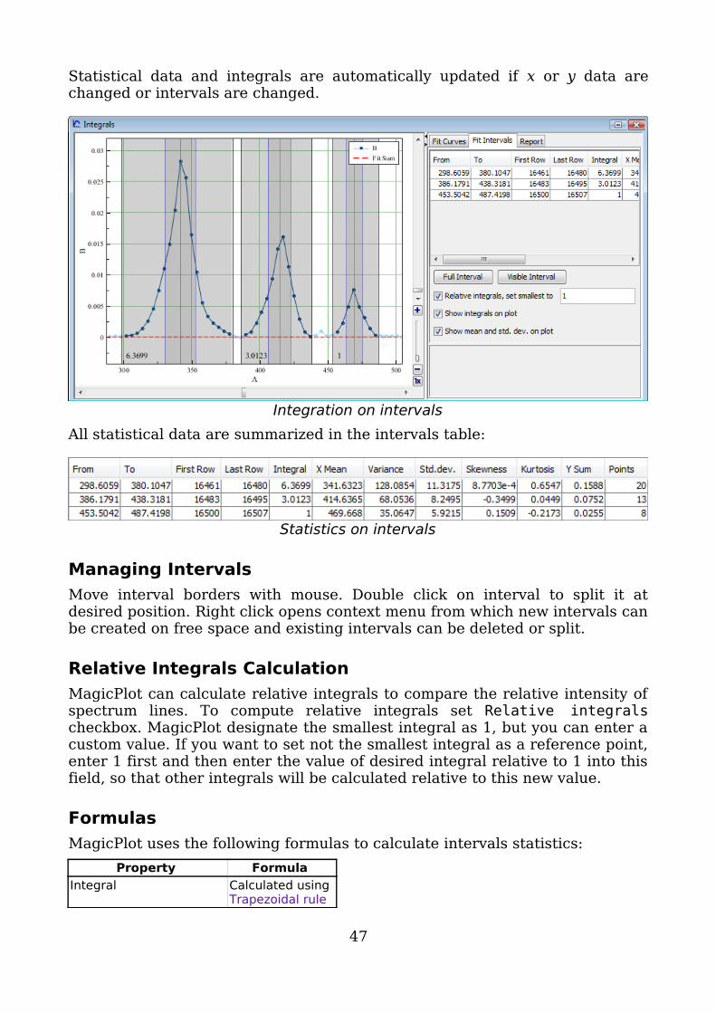
Statistical data and integrals are automatically updated if x or y data are changed or intervals are changed.
Integration on intervalsAll statistical data are summarized in the intervals table:
Statistics on intervals
Managing IntervalsMove interval borders with mouse. Double click on interval to split it at desired position. Right click opens context menu from which new intervals can be created on free space and existing intervals can be deleted or split.
Relative Integrals CalculationMagicPlot can calculate relative integrals to compare the relative intensity of spectrum lines. To compute relative integrals set Relative integrals checkbox. MagicPlot designate the smallest integral as 1, but you can enter a custom value. If you want to set not the smallest integral as a reference point, enter 1 first and then enter the value of desired integral relative to 1 into this field, so that other integrals will be calculated relative to this new value.
FormulasMagicPlot uses the following formulas to calculate intervals statistics:
Property Formula Integral Calculated using
Trapezoidal rule
47

X Mean (expected value)
Variance
Standard deviation
Skewness
Kurtosis
Y Sum
Intermediate values are calculated as follows:
Property Formula X Mean
Central moments
See Also• Nonlinear Curve Fitting: Fit Plot• Using Spline for Baseline Subtraction (Pro edition only)• Descriptive Statistics (Pro edition only)
Transform X or Y Fit Plot Data (Pro edition only)You can quickly transform X or Y data on Fit Plot by using Transform Plot Data items in Processing menu. These menu items open set column formula dialog for table column which is used as X or Y. Note that this transformation affects the table with plotted data.
See Also• Nonlinear Curve Fitting: Fit Plot
Formula SyntaxFormula editor is used in the following cases:• Setting Column Formula• Custom Fit Curve• Entering value in any numeric field and in tables• MagicPlot Calculator
48

MagicPlot uses standard IEEE 754 double precision floating-point arithmetic. Double precision floating point takes 8 bytes per number and provides a relative precision of about 16 decimal digits and magnitude range from about 10-308 to about 10+308.
Syntax HighlightingMagicPlot formula editor highlights expression syntax. It also marks matching brackets:
General Rules
Case SensitivityMagicPlot formula translator is generally case sensitive, i.e. you can write sin but not Sin.Note that x and X are different variables. You can use this feature when naming Custom Equation Fit Curve parameters.
Entering Numbers• You can use dot (.) or comma (,) as decimal separator, and separate
function arguments with a semicolon (;) in the following cases:• Cell editing in Tables• Entering value in any numeric field• Using MagicPlot Calculator
• You can use dot (.) only as decimal separator, and separate function arguments with a comma (.) or a semicolon (;), in:• Setting Column Formula• Custom Fit Curve
You can use e or E for scientific notation: 1.45e-3 or 1.45E-3.
Using Spaces and Line BreaksYou can freely insert space characters and line breaks in formula, but do not break function names, numbers, operators. You do not need to enter special characters to indicate line break.
FunctionsYou can see a list of all available functions and their descriptions in Functions tab in Set Column Formula window and in Help on Functions window which can be opened from menu in calculator window.MagicPlot uses functions of Java programming language library StrictMath to
49

evaluate sin, cos, exp, etc. These functions are available from the well-known network library netlib as a “Freely Distributable Math Library”, fdlibm package. The same library is widely used in many scientific computing applications.
Trigonometric FunctionsMagicPlot supports all standard trigonometric functions (sin, cos, etc.). All angles are always measured in radians for clarity. You can use the following functions to convert angles units:• deg(a) — converts angles input in radians to an equivalent measure in
degrees.• rad(a) — converts angles input in degrees to an equivalent measure in
radians.
Examples
• sin(rad(90))• deg(asin(1))
ConstantsThe predefined constants are:• pi, Pi, PI — π = 3.1416… value (the ratio of circumference of a circle to
its diameter).• e — e = 2.7183… value (the base of the natural logarithms). Note:
expression e^a is evaluated as exp(a).• nan, NaN, NAN — Not-a-Number value.• inf, Inf, infinity, Infinity — positive infinity value which may be used in
some calculations. Note: write -inf for negative infinity.• eps — machine epsilon, gives an upper bound of the relative error due to
rounding in floating point arithmetic. Note: eps = ulp(1) = 2^(-52) = 2,2204E-16. (52 is the number of bits used to store fractional part of a number.)
Boolean LogicMagicPlot can interpret boolean logic expressions. Zero and negative values (<=0) are interpreted as false and positive values (>0) are interpreted as true similarly to C programming language. You can use simple logical operators which are described below. Use 1 as true and 0 as false.
'if' FunctionThe basic logical function is if(condition, a, b). If condition argument is
50

true (greater than 0) it returns the second argument (a), else returns the third argument (b).
Examples
• if(col(A) >= 0, col(A), -col(A)) — evaluates absolute value of column A (you can use abs(col(A)) for that, of course).
• if(col(B) >= 0, col(B), NaN) — returns only positive values from column B. Negative values are replaced with NaN value (empty cell). You can use this expression to filter negative values if you do not want to use them in future calculations. Note that ”Not-a-Number returned at row #” warning can be shown for such expression.
• if(col(A) > 0 & col(B) > 0, max(col(A), col(B)), NaN)
Equality CheckingYou have to be careful if you need to check equality of two values. Due to inaccuracy of computer floating-point calculations the result of evaluation is always approximate. For example, result of sqrt(3)^2 is number 2.9999999999999996, not exactly 3. The expression sqrt(3)^2 == 3 is false (it returns 0). Keep in mind that for convenience MagicPlot rounds numbers when showing on the screen, so this value will be shown as 3 in table if the number of shown fractional digits in MagicPlot preferences is not big enough.Generally, if you want to check equality of two values you need to use some equality threshold for relative difference. That is, you should compare the modulus of relative difference of two values a and b with threshold t: if(abs((a-b)/a) < t, …, …).
Examples
• sqrt(3)^2 - 3 results something about -4,4409E-16• if(abs(sqrt(3)^2 - 3) / 3 < 1e-10, …, …) — checks equality of sqrt(3)^2 and 3 with a threshold of 1e-10.
OperatorsOperator Description Operator Description + addition == equal to - subtraction != not equal to * multiplication < less than / division > greater than ^ power <= less than or equal to | or >= greater than or equal to & and
Operations PriorityOperators with lower precedence value are evaluated earlier. You can use brackets to change calculation sequence.
51

Expression is evaluated left-to-right, excluding repeated exponentiation operator ^. The ^ operator is right-associative like in Fortran language (evaluated right-to-left; note that in general case a^(b^c) ≠ (a^b)^c). Hence a^b^c is evaluated as a^(b^c). The reason for exponentiation being right-associative is that a repeated left-associative exponentiation operation would be less useful. Multiple appearances could (and would) be rewritten with multiplication: (a^b)^c = a^(b*c).
Operations Precedence Associativity () (function call) 1 — ^ 2 Right-to-left - (unary minus) 3 — *, / 4 Left-to-right +, - 5 Left-to-right <, >, <=, >= 6 Left-to-right ==, != 7 Left-to-right & 8 Left-to-right | 9 Left-to-right = (assignment) 10 Left-to-right
Examples
• 1 + 2 * 3 returns 7.• (1 + 2) * 3 returns 9.• 2*-3 returns -6.• -3^2 is equal to -(3^2), because ^ priority is higher than that of unary
minus. The result is -9.• (-3)^2 returns 9.• 2^2^3 is equal to 2^(2^3), because ^ is right-associative operator. The
result is 256.
Table SortingTo sort Table select Table → Sort Table menu item. You can sort the entire table or only selected area (columns and rows selection). You can also use Sort by This Column item in Table context menu (exactly one column must be selected).
52

Sorting Criteria
Sort table dialogYou may specify multiple sorting criteria columns. If the value in the first criteria column are the same MagicPlot will compare the values from the second criteria column if specified.
53

Visual Data NavigationScale Scrolling for Data NavigationMagicPlot provides useful plot data navigation (scale scrolling and zooming). Here are several tools and methods:• Mouse wheel rotation inside the current Axes box scrolls x/y or zooms x/y
scale. Ctrl and Shift keys toggle the mode• Scale box zoom tool• Hand tool (only if the image zoom is 1x, otherwise the while image will be
scrolled in window)• Right mouse button dragging always works as Hand tool (except Mac OS X)• The scrollbars (only if the image zoom is 1x, otherwise the while image will
be scrolled in window)• Scale buttons on the toolbar.
Scale and tools buttons
Do not Confuse Scale Scrolling and Image Zoom• Scale scrolling affects the x/y scale minimum and maximum values. Use
scale scrolling for data navigation• Image zoom enlarges the entire image (Pro edition only). Use image zoom
for accurate drawing of small objects.
Current AxesIf your Figure contains more than one Axes box, MagicPlot indicates which Axes are currently selected with blue circle sectors in the corners of Axes box. The current Axes selection affects the action of scale buttons and Add to Selected Axes item in Table context menu. It also helps you to distinguish the Axes when you change style in the Figure Properties dialog window.
Axes selection buttons
54

See Also• Drawing on Figures and Fit Plots, Image Zoom and Objects Selection• Reading Plot Data, Measuring Distances, Curves Selection
Reading Plot Data, Measuring Distances, Curves SelectionMagicPlot shows mouse cursor data coordinates in status line. If you have several axes on one Figure, cursor coordinates relative to selected axes are shown.
Crosshair CursorMagicPlot can draw crosshair cursor. To turn it on use View → Crosshair Cursor menu item.
Crosshair cursor and its coordinates
Reading Plot DataMagicPlot denotes the data point under the mouse cursor with square brackets. The accurate table value in this point along with table name, row and column numbers is shown in status line in the bottom of main window in the following format:Folder | Table [x column; y column][row] = (x value; y value)
55

Reading plot data
Curve Context Menu
Curve context menu on FigureUse context menu of the Curve to open table with data or to open properties dialog.
Measuring Data Distances with Scale Zoom ToolYou can use Scale Zoom tool to measure the distances on plots. MagicPlot shows the distance in status line when you select zoom box by mouse dragging. You can press Esc or reduce box size to zero before releasing mouse button to prevent zooming if you want only to see the distance. If multiple axes are located under cursor MagicPlot will show the distance in terms of current axes (showed with blue corners).
56

Distance measurement
Selecting Curves in Turn Using KeyboardCurves on Figures and Fit Plots can be selected with mouse click. You can also select Curves in turn using Arrow keys or Tab/Shift+Tab keys:• → or ↓ or Tab selects the next Curve• ← or ↑ or Shift+Tab selects the previous Curve.If no Curves are selected the first pressing on these keys will select the first Curve. If the Figure contains multiple Axes, the Curves in all Axes are accessible in turn by this method.
Curve 1 is selected
57

Curve 2 is selected
See Also• Scale Scrolling for Data Navigation
Quick Plot ToolQuick Plot tool is used for viewing a plot of Table columns without adding new Figures to Project. Select Tools → Quick Plot item to open this tool.
Quick Plot toolWhen Quick Plot window is open select some columns in Table to view the plot.
58
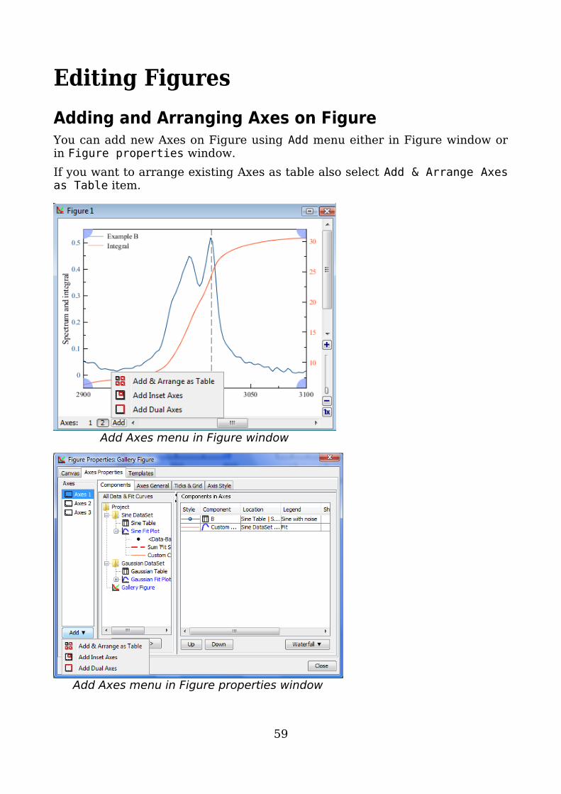
Editing FiguresAdding and Arranging Axes on FigureYou can add new Axes on Figure using Add menu either in Figure window or in Figure properties window.If you want to arrange existing Axes as table also select Add & Arrange Axes as Table item.
Add Axes menu in Figure window
Add Axes menu in Figure properties window
59

Add and Arrange Axes as Table
Arrange Axes as table dialogThis dialog may be used also to arrange existing Axes without adding new Axes.
Adding and Arranging Curves on Figure AxesThe best way to create a Figure with desired data is to select x and y data columns in Table and use Create Figure in Table context menu.There are different ways to add data to existing Figure:• Select x and y columns in table with data, open table context menu (right
click) and select Add to Selected Axes sub-menu. All currently opened Figures are listed in this sub-menu.
• Open Figure Properties window and go to Axes Properties → Components tab. Here you can select the Table in the project tree and press Add to Axes button.
You also can add Fit Curves or Fit Sum from Fit Plot to Figure.
Changing Curves Drawing OrderTo change Curves drawing order and legend entries order open Figure Properties dialog and go to Axes Properties → Components tab. Drag rows in table to reorder. You can also use Up and Down buttons or press Alt + up/down keys (Option + up/down keys on Mac) to move selected row in table up or down.
60

Curves reordering in Figure properties dialog
Shifting Curves on Figure and Creating 2D WaterfallMagicPlot allows you to set individual x and y shifts for every Curve on Figure. This feature may be used to compare several similar Curves on one Figure.
61

2D Waterfall FigureSpecified Curve shifts do not affect your data and are used only for drawing current Figure.Curve shifts can be set in X Shift and Y Shift columns in Axes Components table (scroll table right if these columns are not visible). Waterfall menu contains items for making and resetting 2D waterfall and reversing curves order.• Reset Shifts sets all x and y shifts to zero• Make Waterfall automatically calculates shifts and arranges CurvesMake Waterfall menu item opens waterfall window in which you can specify shift increment. MagicPlot tries to guess handsome shift values on the basis of number of curves and current scale.
Waterfall window
62
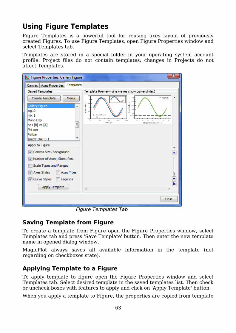
Using Figure TemplatesFigure Templates is a powerful tool for reusing axes layout of previously created Figures. To use Figure Templates, open Figure Properties window and select Templates tab.Templates are stored in a special folder in your operating system account profile. Project files do not contain templates; changes in Projects do not affect Templates.
Figure Templates Tab
Saving Template from FigureTo create a template from Figure open the Figure Properties window, select Templates tab and press 'Save Template' button. Then enter the new template name in opened dialog window.MagicPlot always saves all available information in the template (not regarding on checkboxes state).
Applying Template to a FigureTo apply template to figure open the Figure Properties window and select Templates tab. Select desired template in the saved templates list. Then check or uncheck boxes with features to apply and click on 'Apply Template' button.When you apply a template to Figure, the properties are copied from template
63

to Figure. Note that the Figure style will not be changed if you change the template after you have applied it to Figure. The project file is standalone and you do not need the template to open project.You can undo applying template in a standard manner (no need to close the Figure Properties window).
64

Drawing and EditingAxes Style EditingAxes style can be set in Figure Properties window (or Fit Plot Properties for Fit Plot). This window contains multiple tabs with axes drawing settings.
Figure Properties window
Drawing on Figures and Fit Plots, Image Zoom and Objects SelectionYou can draw the following kinds of objects on Figures and Fit Plots (Pro edition only):• Text labels with formatting support• Lines• Arrows• Rectangles• Ellipses
65

Select an appropriate instrument in the toolbar to draw an object.The properties of selected objects can be changed in the inspector toolbar (the second row of toolbar).
Image Zooming (Pro edition only)If you need to precisely draw some small objects you can zoom in the image using slider in right bottom (Pro only).There are several alternative ways to change the image zoom:• Scroll the mouse wheel at the image zoom slider• Ctrl+scroll (Cmd+scroll on Mac) mouse wheel at blank part of plot (outside
all axes boxes)• The button 1x and Alt+click (Option+click on Mac) on plot fits the image to
the window.
Image zoom slider and buttons
Do not Confuse Scale Scrolling and Image Zoom• Scale scrolling affects the x/y scale minimum and maximum values. Use
scale scrolling for data navigation• Image zoom enlarges the entire image (Pro edition only). Use image zoom
for accurate drawing of small objects.
Objects selectionEvery object can be selected by clicking on its border or inside it. Hold Ctrl key (Windows, Linux) or Shift key (Mac OS) and click another object to add it to current selection.
66

Moving an Object Forward or BackwardWhen objects overlap, you can change the order of objects drawing. Use Bring to Front and Send to Back items in object context menu (right click on object to open menu).
Ellipse context menu
Changing Curves Order on FigureYou can change the order of drawing the curves on Figure. The curves order can be set in Figure Properties window, Axes Properties tab → Components tab. Select desired curves in list, then hold Alt and press up/down arrow keys. You may also use Move Up and Move Down items in Waterfall button menu.
Snapping to Other ObjectsWhen you drag an object or change its size, MagicPlot will try to snap the bounds of this object to other objects. While snapping MagicPlot shows you a red ruler and an object to which the bounds are snapping. If you do not want to align your objects this way, hold Ctrl key to disable snapping.
Snapping to other objects
67

See Also• Scale Scrolling for Data Navigation• Reading Plot Data, Measuring Distances, Curves Selection
Colours and Opacity AdjustmentIn MagicPlot you can set the opacity of each object (curve, text label, rectangle, etc.) to make it semi-transparent. Opacity is treated as a property of object color. You can set opacity in Opacity sub-menu in color pop-up menu which opens by clicking on color button. Opacity percentage is shown on colour button.
Color pop-up menu
See Also• Creating Transparent Figures and Fit Plots
Creating Transparent Figures and Fit PlotsTo create an image with transparent background open Figure Properties or Fit Plot Properties dialog window and set Transparent Background radio button in Canvas tab.The background of transparent Figures and Fit Plots is shown with a grey-and-
68

white chequerboard. If you are preparing a picture for a dark background you can change the colour of chequerboard to dark grey by selecting View → Transparency Checkerboard in main menu.In case of transparent background you can set the preview background colour in Image Preview window.
Transparent figure example
See Also• Colours and Opacity Adjustment
Using of Drawing Dimensions ToolbarThis toolbar is intended for precise setting of the position and size of one or more selected drawn objects on Figure or Fit Plot.You can open Drawing Dimensions toolbar by selecting Tools → Drawing Dimensions in main menu. Drawing Dimensions toolbar may be left opened.
Drawing Dimensions toolbar
Drawing Dimensions toolbar shows the coordinates and size of currently selected object(s). You can also specify the coordinates or size of several components.• The x value is measured from the left edge of the canvas.• The y value is measured from the top edge of the canvas.
69

• For rectangle or ellipse the specified coordinates determine the position of the upper-left corner.
• For text label:• x determines the left edge, center or right edge of text according to text
alignment of label.• y determines the baseline position of the first line.
• For line or arrow the specified coordinates determine the position of the beginning.
Switching Curves Antialiasing on the Screen
Antialiasing off Antialiasing on
You can toggle curves antialiasing (smoothing) by selecting View → Curves Antialiasing in main menu.Please note that antialiasing may slow down the drawing if you have many data points (~100K).
70

Text Labels EditingInserting Special Symbols and Greek LettersMagicPlot supports any Unicode symbols, including Greek letters and many special symbols.The help on inserting Greek letters and special symbols is also available in Help menu.
Typing Greek letters with Keyboard ShortcutsTo insert Greek letter type Ctrl+G (Command G on Mac OS) and then type Latin letter mentioned in the table below.Greek Letter Name Greek Symbol On Keyboard
(Ctrl+G, then)
Alpha Α α A a Beta Β β B b Gamma Γ γ G g Delta Δ δ D d Epsilon Ε ε E e Zeta Ζ ζ Z z Eta Η η H h Theta Θ θ Q q Theta (alt.) ϑ J Iota Ι ι I i Kappa Κ κ K k Lambda Λ λ L l Mu Μ μ M m Nu Ν ν N n Xi Ξ ξ X x Omicron Ο ο O o Pi Π π P p Rho Ρ ρ R r Sigma Σ σ S s Tau Τ τ T t Upsilon Υ υ U u Phi Φ φ F f Phi (alt.) ϕ j Chi Χ χ C c Psi Ψ ψ Y y Omega Ω ω W w
Inserting Math Symbols with Keyboard ShortcutsTo insert math symbol type Ctrl+M (Command M on Mac OS) and then type symbol mentioned in the table below.
71
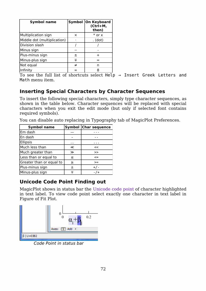
Symbol name Symbol On Keyboard (Ctrl+M, then)
Multiplication sign × * or x Middle dot (multiplication) · . (dot) Division slash ∕ / Minus sign − - Plus-minus sign ± + Minus-plus sign ∓ = Not equal ≠ n Infinity ∞ 8 To see the full list of shortcuts select Help → Insert Greek Letters and Math menu item.
Inserting Special Characters by Character SequencesTo insert the following special characters, simply type character sequences, as shown in the table below. Character sequences will be replaced with special characters when you exit the edit mode (but only if selected font contains required symbols). You can disable auto replacing in Typography tab of MagicPlot Preferences.
Symbol name Symbol Char sequence Em dash — --- En dash – -- Ellipsis … ... Much less than ≪ << Much greater than ≫ >> Less than or equal to ≤ <= Greater than or equal to ≥ >= Plus-minus sign ± +/- Minus-plus sign ∓ -/+
Unicode Code Point Finding outMagicPlot shows in status bar the Unicode code point of character highlighted in text label. To view code point select exactly one character in text label in Figure of Fit Plot.
Code Point in status bar
72

See Also• Advanced Typography Features
Advanced Typography FeaturesMagicPlot provides accurate typography in text labels and axes labels. You may toggle some features in 'Typography' tab of MagicPlot Preferences.
Typography tab in MagicPlot Preferences window
Ligatures SupportMagicPlot supports Latin ligatures in text labels. If you type 'fi', 'fl', etc., those symbols will be shown with ligature glyphs when you exit edit mode.
Edit mode
Result
MagicPlot supports at least the following ligatures:• fi, fl• ff, ffi, fflNot all fonts contain ligature glyphs. MagicPlot displays ligatures only if the glyphs are included in used font. You can turn the ligatures off in MagicPlot preferences.
73

Mathematical Symbols in Axes LabelsThe numbers in scientific notation need two special characters if you want the typography to be accurate: minus sign and multiplication sign. Many graphing software applications which use simplified typography use letter 'x' and hyphen-minus (-) in numbers instead of typographically correct special characters. This simplified typography was mainly used in old applications which do not support Unicode.MagicPlot can use either correct symbols (default) or simplified. You can change this option in MagicPlot Preferences.
Minus SignVarious minus-like characters are used in different cases and have different height and length. The height and length of minus sign are equal to those of plus sign and correspond to the size of digits in the font. Here is a comparison of these characters:
Plus and minus signsWhen you edit some text, keyboard minus key enters hyphen-minus character. The correct minus character can be typed in text label by pressing Ctrl+M, -, see Inserting Special Symbols for details.
Multiplication SignIn different languages, multiplication signs differ. In most cases you have to use either '·' or '×' sign. You also can specify any special character or character sequence, for example enter spaces before and after multiplication signs.
Multiplication sign Correct minus sign
Middle dot Correct minus sign
Simplified typography: Latin letter 'x' hyphen-minus instead of minus
See Also• Inserting Special Symbols and Greek Letters
74

Image Exporting and CopyingImage ExportTo export Figure or Fit Plot image click on Project → Export Image menu item or use corresponding toolbar button. You can set various options of file export format by clicking on Format Options button in Export Image dialog window.You can also copy image to clipboard.
Raster Image FormatsThe following lossless raster graphics formats are supported:• PNG — the most suitable format for Fit Plots and Figures• GIF — supports only 256 colours and no transparency, out-of-date format• BMP — uncompressed raster format (large file size)
Setting the resolution of exported raster imageImage resolution for raster export can be set individually for every Figure and Fit Plot in Canvas tab of the Properties window. The default resolution is 300 DPI.
Why is MagicPlot not capable to export images in JPEG format?JPEG is a commonly used format of lossy compression for photographic images. The JPEG compression algorithm is at its best on photographs and paintings of realistic scenes with smooth variations of tone and color. However, JPEG is not suited for line drawings and other textual or iconic graphics, where sharp contrasts between adjacent pixels cause noticeable artefacts. Such images are better saved in a lossless raster graphics format such as BMP, GIF, PNG or vector graphics formats.
PNG and JPEG Comparison
PNG JPEG
75

Vector Image Formats (Pro edition only)The following vector graphics formats are supported:• PDF• EPS• EMF — the most suitable format for inserting in Windows applications like
Microsoft Office
Export in vector graphics formats by virtual printerYou also can use third-party virtual printer software to export image in vector graphics formats.
See Also• Copying Images to Clipboard (Pro edition only)• Preview Image
Preview ImageUse Project → Image Preview menu item to open image preview window. You can also use the Preview button of the toolbar or Ctrl+Shift+P keyboard shortcut (Cmd+Shift+P on Mac).
Preview FeaturesIn preview mode you can:• Preview in gray scale• Transparent images can be previewed on selected background color• Change the zoom of the image
76

Image Preview window
Preview Zoom OptionsThere are several options for the size of preview:• Percent of real size. Note: The size will be actually real only if the dots
per inch (DPI) is correctly set in your operating system• Fit to Window, Fit Width, Fit Height — fits the size of previewed image
to window dimensions• Pixel-to-Pixel — allows you to see the accurate image that you will get
using export in raster image format. The resolution of exported raster image is evaluated as a product of canvas size and DPI value specified in Canvas tab of Figure/Fit Plot Properties window.
Copying Images to Clipboard (Pro edition only)When you edit a presentation or report, it is very useful to paste images from MagicPlot to another application directly through clipboard without saving them. MagicPlot supports copying images to clipboard in both raster and vector formats from Edit menu. Transferring vector images is always preferable because these images are scaled more precisely. However, we have found that some applications do not support pasting vector images, or paste vector images with distorted text. In this case, please use copying raster image.
See Also• Image Export
77

ToolsMagicPlot CalculatorMagicPlot Calculator is a useful formula calculator built in MagicPlot. To open calculator use Tools → Calculator menu item. Calculator window stays on top when MagicPlot main window is minimized to task bar (Dock on Mac), so you can use the Calculator when working with other applications.
Heron's formula in MagicPlot Calculator
Using the Calculator• Type (12+4)*sin(pi/2) and press Enter to get the result• Type a=5 to set variable a to 5• Use Up/Down keys to recall previously entered expressions• Use ans (Ans) variable or press Ctrl+Up to insert the result of latest
operation• Standard functions and variables (sin, cos, pi, e, etc.) are supportedMagicPlot Calculator uses the same formula syntax as other formula fields in MagicPlot application. Calculator supports comma (,) as decimal separator (1.2 = 1,2), so use semicolon (;) as function arguments separator: min(1;2). MagicPlot Calculator supports user-defined variables.
Standalone Calculator ApplicationMagicPlot Calculator can also be used as a free standalone cross-platform application. You can download it here
78

See Also• Formula Syntax• Download MagicPlot Calculator as a standalone application
79

AppendicesPortable Installation on USB driveYou can copy MagicPlot executable file to your portable USB drive and launch it on some other computer directly from this USB drive, without installation. To do this, you have to copy MagicPlot preferences file to the folder on USB drive which contains MagicPlot executable file. Here are step-by-step instructions:1. Create new folder on USB drive for MagicPlot2. Copy MagicPlot executable file to this folder3. Run MagicPlot4. Exit MagicPlot. It will automatically store preferences file magicplot.ini in
MagicPlot folder in your operating system profile (see below)5. Copy magicplot.ini from MagicPlot folder in your operating system profile
to the folder on USB drive which contains MagicPlot executable.
Where does MagicPlot save preferences in my operating system profile?
• Windows XP: C:\Documents and Settings\<Your account>\Application Data\MagicPlot\
• Windows Vista, 7: C:\Users\<Your account>\AppData\Roaming\MagicPlot\
• Mac OS X: <home>/Library/Application Support/MagicPlot• Unix-like systems: <home>/.magicplot.
MagicPlot Editions ComparisonThe table below shows the comparison of MagicPlot Student and MagicPlot Pro editions.
MagicPlot Student
MagicPlot Pro
Price Free of charge, Non-commercial
usage only
$129 Get free trial
General Multiple operating systems support (Windows, Mac OS X, Unix-like)
+ +
No installation procedure, portable installation is available + + Unicode support in projects + + Undo and redo for all actions (with unlimited depth and history list)
+ +
Import tables from text files (.csv, .txt), import dialog with preview
+ +
80

Double precision floating point tables with copy/paste support to/from other apps
+ +
Built-in formula calculator tool + + Entering expressions in every numeric text field + + Setting column calculation formulas with syntax highlighting and formula history
+ +
Optional auto recalculation of column when data in use are changed
— +
Nonlinear Curve Fitting Multi-peak fitting + + Fitting with sum of different functions + + Predefined Gauss and Lorentz functions and their derivatives
+ +
Visual peaks adjusting (fit initial conditions) + + Visual fitting interval setting + + Y data errors accounting + + Easy subtraction of baseline and peak fitting functions from experimental data
+ +
Copying and pasting Fit Curves from one Fit Plot to another
+ +
Automatic peaks finding by 2nd derivative — + Splines for baseline subtraction with fitting capability — + Specifying custom fit equations — +
Data Processing Numerical integration of peaks in spectrum on specified intervals
+ +
Integration of data — + Differentiation of data — + Fast Fourier transform — + Histograms — + Descriptive Statistics — + Numerical spectrum moments (mean, variance, etc.) calculation on selected intervals
— +
Table Sorting by multiple columns, table transposing — + Plotting Features
Plotting capabilities: lines, markers, drop lines, vertical bars, filling under curve
+ +
Error bars + + Switching curves antialiasing on screen + + Fully customizable style for each axis (ticks, labels, grid, etc.)
+ +
Custom grid lines and labels at specified positions + + Transparent images and translucent colors of every object + + In-place text labels editing with formatting support + + 2D waterfall plots and setting individual shifts for curves + + Image zooming in for precise drawing — + Multiple axes on one figure, aligning axes — + Drawing: text labels, lines, arrows, rectangles, ellipses — + Precise objects positioning with snapping and rulers — + Saving and applying Figure templates — +
81

Data Navigation and Exploration Mouse cursor data coordinates in status bar + + Showing data point and table row numbers for point under cursor
+ +
X and Y scrollbars for data navigation + + Box zoom tool for scale + + Hand drag tool for scale + + Mouse wheel or touchpad scale scrolling and zooming + + Quick Plot tool for viewing plot without adding new Figures to Project
— +
Figures Typography Correct minus and multiplication signs (instead of hyphen and letter x) in exponential notation
+ +
English ligatures support (fi, etc.) + + Tracking + + Inserting special symbols (Greek letters, math symbols, dashes, etc.)
+ +
Image Export Raster images export formats: PNG, GIF, BMP + + Vector images export formats: EPS, PDF, EMF — + Copying of raster images to clipboard — + Copying of vector images to clipboard — +
Usage and Support Commercial usage — + E-mail support (write to support(at)magicplot.com) — +
MagicPlot Student can also be used to view project files created in full-featured MagicPlot Pro edition. In such case some project elements (e.g. Custom fit curve formulas) will not be editable.
Keyboard ShortcutsMagicPlot keyboard shortcuts are almost the same in different operating systems (Windows, Mac OS, UNIX-like). The main difference is in modifier keys used: Ctrl on PC (Windows, UNIX-like) and Command on Mac. Some shortcuts were altered to avoid coincidences with system ones.You can find these keyboard shortcuts in MagicPlot by selecting Help → Keyboard Shortcuts menu item.
Mac Keyboard Symbols
• ⌘ Command (Meta) key• ⇧ Shift key• ⌥ Option (Alt) key• Control key⌃
82

Common ShortcutsWindows and UNIX-like Key Mac OS Key Action Ctrl+O ⌘ O Open project Ctrl+S ⌘ S Save project Ctrl+Shift+S ⌘ ⇧ S Save project as Ctrl+N ⌘ N New project Ctrl+I ⌘ I Import table from text file Ctrl+P ⌘ P Print (image or table) Ctrl+Shift+P ⌘ ⇧ P Preview image Ctrl+E ⌘ E Export image Ctrl+K ⌘ K Open calculator Ctrl+U ⌘ U MagicPlot preferences Ctrl+Q ⌘ Q Quit
Undo/Redo Ctrl+Z ⌘ Z Undo Ctrl+Shift+Z or Ctrl+Y ⌘ ⇧ Z or ⌘ Y Redo Ctrl+H ⌘ H Show command history
window Clipboard
Ctrl+X ⌘ X Cut Ctrl+C ⌘ C Copy Ctrl+V ⌘ V Paste Ctrl+A ⌘ A Select all
Table ShortcutsWindows and UNIX-like Key Mac OS Key Action F2 or Double click Double click Edit cell Ctrl+F2 ⌘ F2 Set or edit column formula F4 F4 Rename column (edit header) Ctrl+Enter ⌘ Return Recalculate column Alt+Drag header (Win/Meta+Drag header on UNIX)
⌥ Drag header Rearrange table columns
Figure and Fit Plot ShortcutsWindows and UNIX-like Key Mac OS Key Action Alt+Enter ⌥ Return Open Figure or Fit Plot
properties window Arrows keys Arrows keys Move selected object(s) by 1
mm Shift+Arrows keys ⇧ Arrows keys Move selected object(s) by 0.1
mm Escape Escape Clear selection Delete or Backspace Delete or Backspace Delete selected objects F2 or Double click F2 or Double click Edit selected text label
Moving and Resizing Drawings Ctrl+Drag object ⌘ Drag object Disable rulers and snapping to
other objects
83

Shift+Drag corners ⇧ Drag corners For rectangle and ellipse: preserve aspect ratio For line and arrow: disable snapping to 0°, 45°, 90°…
Alt+Drag corners ⌥ Drag corners For rectangle and ellipse: stretch relative to center
Text Labels Editing 1 Ctrl+Enter or Shift+Enter ⌘ Return or ⇧ Return Apply changes Escape Escape Apply changes Enter Return New line Ctrl+G, then letter ⌘ G, then letter Type Greek letter (letters
correspondence) Ctrl+M, then symbol ⌘ M, then symbol Type special math symbol
(symbol list) Ctrl+B ⌘ B Bold Ctrl+I ⌘ I Italic Ctrl+O ⌘ O Oblique Ctrl+U ⌘ U Underlined Ctrl+L ⌘ L Align left Ctrl+E ⌘ E Center Ctrl+R ⌘ R Align right Ctrl+J ⌘ J Justify Ctrl+– ⌘ – Subscript Ctrl++ ⌘ + Superscript
Scale Range Scrolling and Zoom Scrolling 2 Scrolling Vertical (Y) scale scrolling Shift+Scrolling ⇧ Scrolling or Horizontal
scrolling Horizontal (X) scale scrolling
Ctrl+Scrolling ⌘ Scrolling Vertical (Y) scale zooming Ctrl+Shift+Scrolling ⌘ ⇧ Scrolling or ⌘ Horizontal
scrolling Horizontal (X) scale zooming
Left mouse button+Scrolling ⌃ Scrolling Proportional (X and Y) scale zooming
Image Zoom Ctrl++ ⌘ + Zoom in Ctrl+– or Alt+Click ⌘ – or ⌥ Click Zoom out Ctrl+* or Ctrl+0 ⌘ * or ⌘ 0 Full view
1 These shortcuts are activated in text label edit mode2 Scrolling here means mouse wheel rotation or touchpad vertical scrolling or scrolling by
other human interface device.
84