mage metrology - nano.geo.uni-muenchen.de · the scanning probe image processor, spip v. 2.2, users...
TRANSCRIPT

The Scanning Probe Image Processor, SPIP V. 2.2
The Scanning Probe Image Processor, SPIP™
User’s and Reference Guide
Version 2.2
Copyright © 1998-2001
mage Metrologywww. i mag emet . co m

The Scanning Probe Image Processor, SPIP V. 2.2
The Scanning Probe Image Processor, SPIP V. 2.2
1
User's Guide 3 Welcome ..........................................................................................................5 Tutorial .............................................................................................................6 Graphical Windows ........................................................................................25 Colors.............................................................................................................27 Markers ..........................................................................................................29 Undo...............................................................................................................31 Histogram.......................................................................................................32 Profiling ..........................................................................................................35 Average Profiling and Fourier ........................................................................42 Advanced Profiling .........................................................................................45 3D Visualization Studio ..................................................................................48 Plane Correction Menu ..................................................................................54 Fourier Menu..................................................................................................58 1D Fourier Analysis........................................................................................62 Lateral Calibration and Unit Cell Detection....................................................65 Lateral Linearity Calibration ...........................................................................67 Z-Calibration and Step-height Measurement.................................................73 Correlation Averaging ....................................................................................75 Rotation..........................................................................................................77 Roughness.....................................................................................................79 Grain Analysis................................................................................................81 Tip Characterization.......................................................................................85 Force Curve Analysis.....................................................................................89 Continuous Imaging Tunneling Spectroscopy ...............................................93 Image Properties Menu..................................................................................95 Batch Processing and HTML Reporting ........................................................97 Multiple Image Analysis .................................................................................99 Options Dialog .............................................................................................100 Reading of Unknown File Formats ..............................................................102 Filter Module ................................................................................................105
Introduction to Filters.............................................................................105 The Filter Menu .....................................................................................106 Filter Templates Menu...........................................................................109 Overview of the Different Filter Types...... Error! Bookmark not defined. Linear Filters............................................. Error! Bookmark not defined. Non-Linear Filters ..................................................................................130 Filter Combination Techniques..............................................................139
ImageMet Explorer.......................................................................................143 The ImageMet Explorer™, Introduction ................................................143 The ImageMet Browser .........................................................................144 Common Tasks .....................................................................................151 Dynamic Capture of Results..................................................................153 The ImageMet Finder ............................................................................154 The ImageMet Reporter ........................................................................156
SPIP Plug In Interface for Programmers .....................................................159 SPIP Plug In Wizard for Microsoft Visual C++ 6.0 ................................161 Borland C++ Builder Example ...............................................................165 SPIP Plug In Wizard for Microsoft Visual Basic 6.0 ..............................167
Reference Guide 173 Fourier Analysis ...........................................................................................175 Detecting Line Profiles .................................................................................176 Detecting Unit Cells .....................................................................................177 Lateral Calibration by Quadratic Unit Cells..................................................178 Lateral Calibration by Hexagonal Unit Cells ................................................179 Lateral Linearity Analysis .............................................................................180 Calibration by Line Structures......................................................................182 Output File Formats .....................................................................................183

The Scanning Probe Image Processor, SPIP V. 2.2
2
Result files ...................................................................................................184 BCR-STM File Format .................................................................................185 Parameter Files............................................................................................186 Roughness Parameters ...............................................................................187 SPIP Plug In Functions for C++...................................................................195 SPIP Plug In Functions for Visual Basic ......................................................198 References...................................................................................................201

The Scanning Probe Image Processor, SPIP V. 2.2, Users Guide
3
User's Guide


The Scanning Probe Image Processor, SPIP V. 2.2, Users Guide
5
Welcome
Thank you for choosing the Scanning Probe Image Processor, SPIP™ the most powerful product for accurate Image Analysis. SPIP is designed with uncompromising attention to the needs of metrology and measurement quality. SPIP includes a number of unique and accurate techniques for automated detection and correction of image distortions not found in other programs. Although containing many specialized functions for Scanning Probe Microscopy, SPIP can successfully be applied for other types of data, for example, SEM, interference microscope, optical microscopy images and even 1 dimensional profiles. If accurate measurements and quality assurance are important issues then, SPIP is the right choice. In addition to detailed surface characterization, SPIP is the most powerful tool for characterizing scanning probe instruments and diagnosing environmental noise and vibration problems. Therefore, SPIP is a valuable data analysis program for many applications and means higher quality and added value for instrument designers as well for end-users within industry and research institutes. We are convinced that you are going to be satisfied with SPIP and we are committed to continue the innovative development of SPIP in close contact with our customers. Should you have additional requirements for new image processing functions, do not hesitate to contact us.
Jan F. Jørgensen
CEO Image Metrology ApS
[email protected] / www.imagemet.com

The Scanning Probe Image Processor, SPIP V. 2.2, Users Guide
6
Tutorial To learn how to use SPIP efficiently we recommend that you run the following tutorial, which will guide you through the most important analytical procedures. If you need help press F1 at any time, or select Help����Help Topics from the menu bar.
There is context-sensitive help for all dialogue menus, just click on the question mark found in the upper right corner of the menu and drag it to the field or button of interest. Quick Introduction Tour The following will give you a quick overview of the features included in SPIP.
Start the Open file dialogue by the associated tool key. If you have ImageMet Explorer installed you will be able to browse for the files in thumbnail view. Now locate the Waffle.bcr image file, which is located in the same directory as the SPIP program and open it by a double click. The result should be a screen similar to the one below:
The image contains a waffle pattern with a repeat distance of 10 µm and step-heights of 100 nm. It is suitable for demonstration of X, Y and Z calibration.
Try to change the colors with the color tool keys: or edit the color lines in the Color Scale Editor. Try also to place the mouse in the color bar of the image or the Color Scale Editor and change the contrast by moving or stretching color bar.

The Scanning Probe Image Processor, SPIP V. 2.2, Users Guide
7
Get a fast calculation of the unit cell (pitch). This will provide a Fourier image and the Unit Cell and Calibration Results dialogue where all results are shown. To get the proper correction parameters enter 1000 nm as the Reference Pitch value and press Apply. Note, that the unit cell is drawn on the image and that you can move it using the mouse or arrow keys, convince yourself about its correctness and investigate the image uniformity.
Click the Oblique maker tool once for seeing just one unit cell and twice for turning off the lattice indication.
Click the key associated with the Fine Linearity Analysis. If you have created a zoom image by the rectangle marker tool this image will be used as a template for finding similar structures in the image. Otherwise, SPIP automatically selects a template based on the calculated unit cell. You should now see that the image has got an overlay of the calculated lattice and some small red arrows indicating the error vectors in relative size.

The Scanning Probe Image Processor, SPIP V. 2.2, Users Guide
8
You can turn off the lattice and error indication by the oblique marker tool. The absolute size of the errors are seen in the Linearity Correction Dialog and in the two scatter diagrams visualizing the linearity error for the X and Y directions:
The results are quantified and reported in the Linearity Correction window and in the Unit Cell and Calibration Results window. It is possible to correct this or other images by the correction parameters. A new estimation of the correction parameters should then result in neutral values, indicating that no further correction is needed.
Click on the toolbar button associated with the fast step-height calibration and a histogram showing peaks corresponding to the two dominant height levels appears:

The Scanning Probe Image Processor, SPIP V. 2.2, Users Guide
9
The histogram also reports the detected step-height and the Z-calibration factor. To get the proper Z-Correction factor the reference step-height for the surface needs to be entered, - this
can be done in the Z-calibration Menu, which is activated by its toolbar button . Try to set the reference value to, for example, 100 nm and press Calibrate, you should then see that the correction factor is changed accordingly. The image you are viewing was already plane corrected when it was loaded by a default third-order polynomial. It is possible to improve this image further by the Plane Correction Menu.
Activate the Plane Correction Menu and observe the instant improvement of the histogram when setting Histogram Alignment on.
The different plane correction methods can be combined to obtain images with minimum distortion, assuring the most accurate Z-calibration.
Click on the roughness key to calculate the bearing curve and a set of roughness parameters. This was the quick tour introducing you to some of the important features. Before continuing with the advanced tour it is a good idea to close the windows, which are not needed any more, this can easily be done by the Window→→→→Close All. Advanced Tour To have an image to work with click on File in the menu bar and select, for example, the Waffle.bc file, which can be found in the most recent files list in the File Menu. You can change the coloring and visualization by the menu items in the View pull down menu or the corresponding icons in the tool bar. Note that you can stretch all image- and curve windows to the size you want. However, the image windows will follow the aspect ratio of the raw image and the width of the images will be calculated based on the height of the window and the ratio between the x and y pixels. The image can also be shown without the colorbar and text: press the right mouse button and select Color Bar On/Off (or CTRL+V)

The Scanning Probe Image Processor, SPIP V. 2.2, Users Guide
10
Try changing the colors by the color toolbar buttons: Alternatively, design your own color table by clicking on one of the red green or blue curves in the Color Scale Editor. When doing so a nail that can be moved by the mouse is created. The color curve will follow the defined nails. You can store the color bar by clicking with the right mouse button and selecting the Store Color Scale command and retrieve other color scales by selecting the Recall Color Scale command. You can also re-scale the image colors by clicking on the color bar below the curves. By doing so, you can define the height values associated with the upper and lower color limits. Let us inspect the image using some of the basic functions:
Create a profile by selecting the Line Drawing toolbar button and draw a line on the image. You will then see the corresponding profile. Change the size of the line by clicking the mouse close to one of the ends. Move the line by selecting a point close to the middle part of the curve. Try to make a diagonal line from one corner of the image to the other. Try also to move the line with the keyboard arrow keys. Select the profile window and use the right mouse key or ‘C’ on the keyboard to activate the cursors, press C twice and you will get two cursor pairs, move the cursors by the mouse or keyboard arrow keys to measure distance and height values. Notice, that the Up/Down arrow keys will locate the locale minimum and maximum positions and the angle of the markers will reflect the slope of the curve.
For easy reading of height and length you may also set the Dimension Readout by the right mouse:
Take a look at the histogram with the two peaks representing the two characteristic height levels of the surface. To measure the height differences manually activate the cursors by the right mouse key. Here it is very convenient to use the key board Up Arrow key to locate the maximums of the histogram.

The Scanning Probe Image Processor, SPIP V. 2.2, Users Guide
11
You should find that the step-height is about 107 nm.
Now let us try to modify the image with the Plane Correction Menu :
The image you see has already been corrected at load time by a third-order polynomial fit based on the average X and Y profile. To obtain the original raw image set Method to None and disable Line-wise Leveling before clicking on the Reload Button. Notice how the image changes and how the changes are reflected immediately in the histogram and the profile. Disable the curve cursors, by pressing ‘C’, if you want to have a more detailed look at the curve and histogram. You can try out the different methods and observe how it affects the image, the profile and the histogram. If Show Difference is checked you will automatically get a difference image for each process. To obtain a good result, select the Least Mean Square method and set the polynomial degree to 3. Enable Histogram Alignment, which will eliminate typical SPM line-wise distortions by raising the individual scan lines to obtain the best histogram match. The result should be a very plane structure with narrow histogram peaks, suitable for accurate Z-height calibration.

The Scanning Probe Image Processor, SPIP V. 2.2, Users Guide
12
Let us continue with the Z-calibration Menu:
In the Z-calibration Menu, you can enter the reference-height for the sample, which in this case should be 180 nm. To obtain a step-height estimate and a Z-correction factor click on the Calibrate button. You will see the results in the histogram window.
For images having step-heights that are small compared to the noise it will often be an
advantage to apply the Correlation Averaging Technique. Pressing the associated tool key starts the correlation averaging. If the zoom image is active SPIP will use this image as the structure that has to be recognized and averaged, otherwise SPIP automatically determines a suitable template based on unit cell detection. You can define a template by the
rectangle marker tool

The Scanning Probe Image Processor, SPIP V. 2.2, Users Guide
13
The selected area will be shown immediately in the Zoom Window:
Press the Calibrate button to calculate the average image, which will be put into the Main Image Window:
You will also see that a standard deviation image has been calculated and that the source image has been saved in another window from where it can be retrieved if desired.

The Scanning Probe Image Processor, SPIP V. 2.2, Users Guide
14
The result is shown in the histogram and the Z-Calibration Menu. Furthermore, the results can be saved in a text file called waffle.bmp.zcal that can be imported to spreadsheet programs, this requires only that you activate this option in the Options dialog.
The advantage of the averaging technique is that it improves the signal-to-noise-ratio by lowering the random noise. Therefore, the analysis will be more robust.
You can get a better impression of the finer structures in 3D view just click once in the average window and click the 3D-toolbar button
In the 3D window you can use the mouse to rotate, move, scale and dynamically change the color properties. With the mouse button down rotate axes the image around the X-and Y-axes by moving the mouse. Hold also down the SHIFT key and rotate around the Z-axis. To scale the image, move the mouse while keeping the CTRL key down. 8 light source can be defined, and is activated by the numerical keys ‘1’ to ‘8’. When combining the numerical keys with mouse movement light source positions can be set conveniently. By pressing ‘A’ or ‘a’ you can start the 3D animation that will display the image at different angles, positions and scaling. See section 3D Visualization Studio for further details on defining the 3D scene. You can get a 3D view for the other images as well. Try to create a 3D view of the original template shown in the zoom image and compare with the average image.

The Scanning Probe Image Processor, SPIP V. 2.2, Users Guide
15
Notice also the Standard Deviation image, which reflects the uniformity (quality) of the structure. Naturally, the standard deviation is highest at the edges of the pit. Before making an analysis of the lateral dimension it is a good idea to close all the windows in order to focus on the important windows you now are going to use.
Open the Waffle.bcr file once more.
Initiate the Fourier transform and the Fourier Menu.
Try to calculate the lateral unit cell by clicking on Oblique Cell as the target structure. The unit cell will be displayed in the main image and you can move it around. You will also get data for the unit cell in the Fourier Menu and in the Unit Cell and Calibration Results Window. The latter also calculates lateral correction parameters. To get the proper correction factors enter 10000 nm as the reference pitch and click on Apply. You can correct any image by this set of correction parameters. It is a good Idea to record the correction parameters for different measurement conditions and apply them when necessary. The calculation is based on the Fourier peaks defining the reciprocal unit cell. When the Fast Peak Detection is disabled, you achieve the highest accuracy because the Fourier peaks are found at sub-pixel level by a sub-pixel Fourier algorithm. Otherwise, the peak positions are estimated by parabolic fits.

The Scanning Probe Image Processor, SPIP V. 2.2, Users Guide
16
To analyze the Fourier image in detail it is an advantage to use high contrast colors. The contrast may also be changed by the SquareRoot or Square functions found in the Fourier Menu and in the Right Mouse Menu. Now, try to detect the unit cell semi-automatically: set the Circle Function in the Fourier Menu to Defines Peak 1 and draw a circle around one of the innermost Fourier peaks associated with the reciprocal unit cell. Notice that the circle will snap its center to the highest point within the circle. Then set Defines Peak 2 on and mark a circle around one of the other innermost peaks (this point should not be on the line with Peak 1 and the origin) You have now defined two corners of a reciprocal unit cell and SPIP does the rest for you, it finds the spatial unit cell and the corresponding lateral correction parameters if a correct pitch reference value has been entered. The co-ordinates of the two peaks are given in the Fourier Menu together with their corresponding wavelengths and the frequency measured in Hz. The latter is very useful for diagnosing phenomena caused by noise.
The waffle.bcr image is also well suited for calibrating the linearity of your instrument:
Click the rectangular marker tool and draw a rectangle about the size of the unit cell or smaller. The area should include a characteristic structure, for example, the corner of a pit. The zoom window will appear and display the selected area.
Start the fine linearity analysis. From the cross correlation function SPIP will at sub-pixel level find the positions of all structures similar to the content of the zoom window. It will compare the positions with those predicted from the unit cell data. The differences are described as linearity errors, which are further minimized by tuning the unit cell (now in the spatial domain). The results is shown in the Linearity Correction Menu:
Consequently, we have not only quantified the non-linearity but also found the best-fit unit cell. Experiments have shown that this gives a better reproducibility than the faster Fourier method. However, the Fourier method is needed for getting a good initial estimation of the

The Scanning Probe Image Processor, SPIP V. 2.2, Users Guide
17
unit cell. The overall linearity error Mean Position Error is also shown in Linearity Correction Menu and more detailed information can be retrieved from the waffle.bcr.linc file. The correction parameters are based on a third-order polynomial model of the scanning system. You apply the correction parameters on the main image by clicking on Correct. Recheck the linearity by clicking on New Estimate and you should observe that the correction parameters become more neutral and that the errors in the scatter diagram reduce to the sub-pixel level, and that the Mean Position Error decreases.
When calculating a new Fourier image you will also notice that the Fourier peaks have become sharper, especially the weaker peaks close to the border. Try also to correct the physical scaling and orthogonality of the image using the Unit Cell and Calibration Results dialog. Enter 10 000 as the Ref. Pitch La reference pitch value and click on the Apply button and you will notice that the correction parameters changes accordingly. Then click the Correct button to get a corrected image. Analysis of Self-Assembled Molecules Now let us try to analyze an image containing didodecylbenzene molecules self-assembled on a graphite substrate:
Check first the plane correction settings, disable Line-wise leveling, which will be applied when loading the file, close all windows (Window→→→→→→→→Close All)
Open the ddb.bcr image file:
Get a quick calculation of the unit cell. You will notice that the calculated unit cell covers parts of more molecules and that a unit cell not necessarily equals the shape of the molecules. There are more alternative unit cells the default selected by SPIP is one having the angles closest to 90°. To get a unit cell closer to the shape of the molecule activate the Fourier Menu and click on the <a = a + b> button four times. Try also the other arithmetic buttons.
Make a zoom image by the rectangle marker tool choose a representative area covering more molecules:

The Scanning Probe Image Processor, SPIP V. 2.2, Users Guide
18
Calculate an average image by the Processing����Average→→→→Marked area, which will result in an average image and its corresponding Standard Deviation image:
The average image has a much better signal-to-noise ratio and provides more detailed information about the inner molecular structure. The SD image provides important information about structural uniformity. Here, the low SD values at the right part of the benzene rings indicates that this part of the molecule is the part most fixed to the substrate. To create a nice presentation of the result you can show the average image in 3D; Click on the average image with the right mouse key and select 3D:
Another way to filter out unwanted noise without removing the specific Frequencies is to remove only the Fourier components having smaller amplitudes than a value you define by the color bar:

The Scanning Probe Image Processor, SPIP V. 2.2, Users Guide
19
By moving the lower limit of the color bar you define all Fourier components shown as black to be removed when performing an inverse Fourier transformation. If the color bar is not shown in the Fourier window it can be clicked on by CTRL+V otherwise you can also change the limits for the Color Scale Editor. Click on the Inverse button in the Fourier menu and you should see an improved image with the contrast preserved (be careful no to filter too much):
You can also perform interactive filtering by excluding certain areas defined by the marker tools. To perform low-pass filtering enable Center at Origin in the Fourier Menu and mark a circle with the Circle marker tool. Note, that the wavelength corresponding to the circle radius is written simultaneously in the lower right part of the SPIP program window. Click on Include Only:

The Scanning Probe Image Processor, SPIP V. 2.2, Users Guide
20
The filtering will first take place when you click in the Inverse button until then you can undo the exclusions by the Undo button. However, the current change in the Fourier image will have effect on the unit cell detection algorithm, which will ignore the excluded areas. Therefore, you can also use this technique to force the program to find other structures than the unit cell, for example, super structures by ignoring the dominating waves as demonstrated below. To perform band-pass filtering you can mark a new circle inside the previous marked circle and click on Exclude AOI (exclude Area Of Interest, which is the opposite to of the Include Only function).
Open the file ddbsuper.bcr to get a demonstration of a super structure analysis:
This is also an image of DDB self-assembled molecules, now with a more visible super structure.
Calculate a new Fourier image where you will see that main Fourier peaks have satellites associated with the super structure.
Make a fast calculation of the unit cell.
Activate the Oblique maker tool and draw a parallelogram around the inner peaks and their satellites:

The Scanning Probe Image Processor, SPIP V. 2.2, Users Guide
21
Click on Include Only to ignore all Fourier components outside the marked region.
Make an accurate calculation of the unit cell based on the current Fourier image and you will get the super unit cell:

The Scanning Probe Image Processor, SPIP V. 2.2, Users Guide
22
Tip Characterization and Deconvolution Tutorial The following will demonstrate a tip characterization based on a tip characterizer sample, it has only meaning for SPM and stylus instruments:
Open the file tiptest.bcr:
From other images is known that the surface only consist of single tips therefore the observed double peaks can only explained by a probe having a double tip.
Click on the Tip Characterize tool key. To define a suitable size of the tip area to be calculated set the size parameters to 21 x 21 pixels, this will cover the most interesting part of the tip. In this particular case it is important that it is large enough to cover the double tip pair:

The Scanning Probe Image Processor, SPIP V. 2.2, Users Guide
23
Click on Characterize to calculate the tip; this will cause several windows to appear, the most important one is the image of the estimated tip and by clicking the View Tip in 3D checkbox a 3D tip image will be created:
To get the best impression of the tip form it can be an advantage to use a combined wire-frame view as shown above; this is set in the 3D Visualization Settings dialog. Note, that the relative flat outer part of the tip image not necessarily reflects the true shape of the tip. The problem is that the actual image does not possess enough information to extract a larger part of the tip. However, in most cases it is only an area within a radius of a few hundred nanometers that is important for the imaging process. Now, that we have a good knowledge of the central part of the tip we can reconstruct the surface image; now press Deconvolute. The resulting image will be shown in the Main

The Scanning Probe Image Processor, SPIP V. 2.2, Users Guide
24
Image window while the original for convenience is stored in another window. It should now be observed that the double tip artifact now has disappeared. For comparison it is a good idea to view the original and the corrected image in 3D, just press ‘3’ in the 2D image window you want to view in 3D:
Original Image
Image after Tip Correction
The demonstrated technique is not limited to the use of dedicated tip characterizers. What qualifies a good tip characterizer sample is that it possesses features in all directions having slopes larger than the tip; the structure does not need to be systematic or known in advance. Also, once knowing the tip shape it can be stored and used for deconvolution on other images.
End of tour This was the end of the tour. There are still a lot of other advanced features to explore and we hope that you now feel inspired and encouraged to use SPIP on your own images!

The Scanning Probe Image Processor, SPIP V. 2.2, Users Guide
25
Graphical Windows Different types of graphical windows may be created during a SPIP session:
• The Main Image window, • 3D Image Window, • Fourier Image Window, • Zoom Image Window, • CITS Image Windows • Profile Window, • Force Curve Windows • 1D Fourier Window, • Histogram Window, • Bearing curve (Abbott), • Polar Plots, • Grain detection window, • Linearity Scatter Diagrams and the • Color Scale Editor.
Except for the Color Scale Editor, all windows depend on real data. Some functions can only be calculated based on the main image, for example, Fourier transform, slope correction, lateral and vertical calibration, roughness calculation, histogram calculation and averaging. For the other image windows, the functionality is limited to the zoom function, profiling and a few other operations. However, it is possible to transfer any image to the main image window by use of the right mouse key and utilize all the functionality of the main window. The Fourier window has a lot of additional functionality that can be activated by use of the Fourier Menu. Windows pull-down menu The Windows pull-down menu can control the organization of the windows:
Tile Automatically The menu contains the option to auto tile the graphical windows whenever a new window is created so that all windows are visible and not overlapping. Tiling Modes The windows can be tile by the Tile Best Fit Method where SPIP tries to figure out how to use the space best as possible or in 1,2,3 or 4 columns. Or the number of columns can be fixed to 1, 2, 3 or four by the associated keys.

The Scanning Probe Image Processor, SPIP V. 2.2, Users Guide
26
Closing Windows When working with more images and performing different types of analysis the number of windows can grow so high that it can be difficult to navigate and find the specific windows, therefore SPIP has included convenient functions for closing specific groups of windows. For example Close All Except Main will close all SPIP client windows except the Main Window. Windows Appearance All windows can be resized simply by dragging a corner or border with the mouse. Image windows will be adjusted so that the x-y aspect ratio equals the aspect ratio of the physical dimensions for curve window the aspect ratio can be defined differently. Note, to achieve the best accuracy the raw image data is saved in floating point and the graphical output is calculated by interpolation and transferring raw image data into colors. Thus, the raw data is not affected by changing the window size or coloring. The appearance the windows can also be controlled from the Right Mouse Key menus, which are activated by right mouse clicks or from the property menu, which is activated by a double click.

The Scanning Probe Image Processor, SPIP V. 2.2, Users Guide
27
Colors SPIP has four predefined color scales, determining how the height values are visualized. The associated tool keys can activate them:
You can edit the color scale easily by the Color Editor window. The window contains three curves: red, green and blue. The colors of the color bar in the lower part of the window are determined by the y-values of the red, green and blue curves. The resulting colors will be a mixture of the relative RGB values.
The curves contain nails, which the curves are forced to follow. The mouse can move the nails and new nails can be defined. Between the nails, the curves are linear. On a mouse click, the curve closest to the click point will get a new nail at the click point. You can store the color scale by clicking with the right mouse button and selecting the Store Color Scale command and retrieve other color scales by selecting the Recall Color Scale command.
It is possible to define a default startup color scale by storing the color scale into the Default.col file. When no Default.col file exists the Brown Color scale is applied at startup. The color bar at the bottom works together with the color bars of the images. It is possible to move the lower part of the color bar to the right and thereby turn all the lower colors to the minimum color (usually black). This will give a higher contrast for the middle height values. Likewise, the right end of the color bar can be moved to the left, when clicking on the right side of the color bar. Positioning the mouse pointer in the middle part of the bar can move the entire color bar. The same procedure can also be performed on the color bars of the images where the mouse sensitive parts of the color bar are indicated by triangles. Because the modification of the color bar is reflected simultaneously in the Main Image and the Fourier image you can use the color bar as a WYSIWYG interface to the definition of threshold values for Grain analysis, Fourier filtering. Outlier Filtering. By setting the Update All Windows in the right mouse menu the other 2D Windows will adapt the changes as well. For the 3D visualization studio the colors will follow the Color Editor for the default settings.

The Scanning Probe Image Processor, SPIP V. 2.2, Users Guide
28
Color Equalization The Color Equalization mode of an image is toggled by right-clicking Color Equalize in the image window or just by pressing CTRL +Q. Because the color bar by default covers all the height valued of and image the contrast can be weakened by and outlier values causing small features to be invisible. In such cases it can be very useful to apply Color Equalization, which will cause all the different colors to be distributed equally. This will have the effect that the contrast of the small corrugations will improve dramatically. It is also a strong tool for evaluation of small plane distortions and plane correction. The disadvantage is that the transformation is highly nonlinear and does not provide the correct feeling for the height differences.

The Scanning Probe Image Processor, SPIP V. 2.2, Users Guide
29
Markers SPIP has five marker shapes that can be used for marking specific areas of interest in the images and there are specific functions associated with the markers. The markers can be selected from the markers menu or the toolbar marker buttons:
The Line Marker can be applied to all 2D image windows and will generate a profile curve of the corresponding cross section. On a mouse click, the line end closest to the click point will be move to the click point. However, if the click point is closer to the center of the line it follows the mouse pointer while keeping its length and orientation. In some situations it can be convenient the move the line 1 pixel at a time by the arrow keys. The corresponding profile window will be updated simultaneously when changing the cross section line. To make straight horizontal or vertical line you can conveniently combine the mouse movement with the ‘X’ or ‘Y’ keys. When Synchronized Multi Profiling in the markers pull down menu is set it is possible to create a profile for each image window having images of identical size and update them dynamically while moving or resizing the Line Marker in one of the image windows. The Rectangle Marker is used for marking zoom areas and activation of the zoom function. Furthermore, in the Fourier image the rectangle will mark an Area of Interest, which can be modified by the Fourier tools in the Fourier Menu. The rectangle has nine reference points that can be changed by the mouse: The four corners, the center of the four sides, and the center of the rectangle. On a mouse click, the reference point closest to click point will be activated. If the center point is activated the rectangle will be moved while keeping its size. You can also move the box by the arrow keys while monitoring the zoom window. By use of the arrow keys, it is often easier to control the exact position of the zoom box. Synchronized Multi Zoom When dealing with image for the same physical area but showing different properties, for example height, friction, cantilever amplitude, phase, capacitance, magnetic force, etc. it can be very practical to display zoom ins of the different images at the exact same area. This can be achieved enabling Synchronized Multi Zoom in the Markers pull down menu. When active a zoom image for each image window having images of identical size is dynamically updated while moving or resizing the Rectangle Marker in one of the image windows. The Oblique Marker is used to indicate the calculated lattice from a unit cell detection and is default activated after a unit cell detection. It has three modes, which is changed by the oblique marker tool: off, Single Unit Cell mode where only a single unit cell is shown as seen below, - Full Grid where the entire lattice is indicated together with the linearity error arrows if calculated.

The Scanning Probe Image Processor, SPIP V. 2.2, Users Guide
30
The mouse or the arrow keys can move the shape so that it can be compared with the image structure. Alternative unit cells can be defined by the Advanced Fourier Menu. When the oblique marker is active in the Fourier image it is used for marking areas of interest (AOI), - typically an array of Fourier peaks, not parallel to the horizontal or vertical axes. The corners of the parallelogram are defined by mouse clicks: The first mouse click defines the first corner, the following mouse release determines the second corner and on the second mouse click/release the third and fourth corner are defined. The Circle Marker is also dedicated to the Fourier window and additionally to the marking of AOI-s it can initiate the detection of a Fourier peak in the marked circle. In the Fourier Menu you can set the circle function to define Peak 1 or Peak 2 or None. For at defined peak the corresponding x,y and z co-ordinates will be written as well as the corresponding wavelength in nanometer and time frequency in Hz. The latter is useful for detecting electrical noise or environmental vibration. When both peaks are defined they will together with the origin, be regarded as corners in the reciprocal unit cell and the corresponding spatial unit cell will be calculated and displayed in the Fourier Menu. The Angle Measurement Tool Marker is used for measuring angles. The shape and thereby the angle can be changed with the mouse by moving the end positions of the tool marker. The corresponding angle will be written on the screen simultaneously:
When the Mouse Pointer is in a 2D spatial image window, the physical X, Y, Z co-ordinates of that point will be shown in the lower right corner of the SPIP program window:
The unit of the co-ordinates will be the same as for the Actual image. Note, that the X,Y co-ordinates may be negative because they are reflecting the physical co-ordinate system of the image generator. For image files not containing information about the physical co-ordinate system the center of the image is set to (X=0, Y=0) For the Fourier image, the Mouse Pointer will cause the lower right status field to show the wavelength and the amplitude/magnitude of the Fourier component pointed to by the Mouse Pointer:
This indication is useful for wavelength estimation associated with certain Fourier components. In combination with the Circle marker the cutoff frequency for low-pass, high-pass and band-pass filters can be defined.

The Scanning Probe Image Processor, SPIP V. 2.2, Users Guide
31
Undo Each of the image windows can remember up to 9 of the previous images, so than undoing undesired processes is possible. To define the Undo settings click on Undo Settings of the Edit pull down menu:
By selecting the number of images to be saved per image you can find the right compromise between memory consumption and the ability to go many steps back. The Radio buttons determine if the Undo function should be Off, Only active for the Main Image Window or all images. When active functions can be undone by Edit�Undo or Ctrl+z and redone again by Edit�Redo or Ctrl+y.

The Scanning Probe Image Processor, SPIP V. 2.2, Users Guide
32
Histogram The height distribution histogram window is activated by the histogram tool button or from
the Processing�Histogram menu item.
The histogram is an important analytical tool that provides important information about the height distribution and serves as an important tool for the Z-calibration algorithm. It is a good idea to monitor the histogram while performing slope correction because the histogram is the best indicator for the flatness of the surface. Plane surfaces are characterized by high and narrow histogram peaks.
The context menu (right click) contains more functions dedicated to histogram analysis:
Cursors On To activate the cursors right click on Cursors On or just press "C". When pressed repeatable the number of curser pairs will shift between 0, 1, and 2.

The Scanning Probe Image Processor, SPIP V. 2.2, Users Guide
33
The cursors can be moved by mouse and for precise positioning by the arrow keys. The Up/Down arrow keys will move the cursor in the direction of a local summit, which is useful for finding local minimum or maximum points. When a cursor is positioned on a slope, it will be indicated by a tilt of the cursor. Summits are indicated by the cursors pointing straight downwards. Based on the cursor positions you can also determine the area and volume for the range between the markers. Filter Values Outside Markers It is possible to use the blue and red markers for defining the lower and upper clipping values of the image. To perform the clipping right click and select Filter Values Outside Markers. Freeze Axes Right click on Freeze Axes to keep the X and Y scaling fixed. This is very practical when comparing histograms from different images on the same scale. You might for comparison purposes also want to save a duplicate by pressing Ctrl+D. To define the scaling more specifically enter the property menu, by right clicking on Properties or double clicking Show Integration Right click on Show Integration so display the Integration curve of the histogram. The difference between the integration values at the cursor positions reflect the relative surface area having height values between those marked with the cursor pair and will be indicated in the Area% numerical field. Z-Calibrate (Requires the Calibration Module to be included in the license) Right click on Z-Calibrate to perform a step height measurement and calibration, see Z-calibration for further details. Auto Z-Calibrate Right click on Auto Z-Calibrate to automate Z-Calibration measurements whenever the histogram is changed. This is for example practical when the histogram is linked to a profile of an image, in which case both the profile, the histogram and the Z-Calibration result is updated when moving the cross section line in the image. Save As The histogram data can be save into an ASCII file or the STM-BCR file format or as a bitmap file. The ASCII file contains the floating point x, y co-ordinate and can be imported by, for example, spreadsheet programs and the STM-BCR file can be read by SPIP. Copy The window can be copied to the clipboard by pressing CTRL+C and pasted into third party programs by pressing CTRL+V. Duplicate An duplicate of the window can be create by pressing CTRL+D or right clicking on Duplicate Properties Different view options can be defined in the Histogram Properties menu, which is activated by a double click. It is for example possible set the number of histogram bins differently from the default and customize the coloring scheme.

The Scanning Probe Image Processor, SPIP V. 2.2, Users Guide
34

The Scanning Probe Image Processor, SPIP V. 2.2, Users Guide
35
Profiling
The profile window is activated by the Line Marker tool key and is updated simultaneously with movements of the line markers.
Graph Properties The SPIP default view is as shown above, but coloring and other options can be defined and set as new default parameters in the Graph Properties Dialog, which is activated by a double click. The Property menu provides more detailed control of the appearance and functionality of the graphs.

The Scanning Probe Image Processor, SPIP V. 2.2, Users Guide
36
The default parameters will be store along with their associated classes:
• Normal Curve • Histogram • Scatter Diagram • Scatter With Curve • Fourier Graph • Angular Plot
This way the default settings for, e.g., Fourier graphs will be independent from the other curve classes. Below is seen a graph using a different color combination defined from the properties dialog.

The Scanning Probe Image Processor, SPIP V. 2.2, Users Guide
37
Cursors can be activated to make interactive measurements from the Graph Properties dialog or by clicking on the right mouse key and selecting the Cursors On or just by pressing ‘C’ on the keyboard:

The Scanning Probe Image Processor, SPIP V. 2.2, Users Guide
38
By hitting the ‘C’ key twice an extra pair of cursors will be activated. In this mode, it is possible interactively to move the blue and red cursor and get the associated distance and height values written in the yellow box to the right. The red line indicates the most right marker M1 for which the x and y co-ordinate is written. Likewise, values for the lower blue cursor are written. The length and height differences are given in the M2-M1 fields and the effective slope in the dy/dx field in ratio numbers and degrees. Similar readings are seen for the M3 and M4 marker pairs The cursors can be moved by mouse and for precise positioning by arrow keys. The Up/Down arrow keys will move the cursor in the direction of a local summit, which is useful for finding local minimum or maximum points. When a cursor is positioned on a slope, it will be indicated by a tilt of the cursor. Summits will be indicated by cursors pointing straight downwards. Dimension Readout By activating Dimension Readout from the right mouse key menu or the Properties menu, height and distance values will be written between the markers in the profile window:
Show Cursors in Image To view the cursor positions in the source image right click on Show Cursors in Image while inside the profile window:

The Scanning Probe Image Processor, SPIP V. 2.2, Users Guide
39
Define Image Zero Level by Active Cursor; when pressed the image source window will be leveled so that the height at the pixel corresponding to the active cursor becomes zero. This can be practical for setting a reference plane and making it easier to make direct comparisons of multiple images. Freeze Axes; when set on the scaling of the x and y axes will keep their current form even when the newer profiles are exceeding the limits. Otherwise the axes will automatically be adjusted to the current profile. The scaling can also be defined numerically in the Curve Properties menu. Curve zoom is done easily by a zoom box that is handled similar to the zoom box of an image window. Just press ‘Z’ and move and resize the zoom box while the zoomed area is updated simultaneously in the corresponding zoom window.
Curve fitting is default performed automatically by a third order polynomial but can be toggled On/Off by the ‘F’ key or the right mouse key menu. Like wise it is possible automatically to subtract the estimated fit from the input curve by clicking Subtract Fitted Curve on. The polynomial order can be defined in the Properties menu activated by a double click. Quadrangle Fit; Set this option on for fitting a quadrangle to the actual curve. The fit will automatically be updated when the curve changes, see Advanced Profiling for further details. Curve filtering can be activated by the Filter tool key or from the right mouse menu, this will define the actual window as the Filter Source Window. Any changes in the Filter Dialog will apply to the curve window until filtering of another curve or image window is selected as the Filter Source Window.

The Scanning Probe Image Processor, SPIP V. 2.2, Users Guide
40
Filter Auto Apply; When set on this option will cause the selected filter to be performed whenever the profile data changes. This may for example be practical when moving the cross section line in the source image. Histogram; Press Histogram to create a height distribution histogram of the profile, see further details in the Histogram section. Histogram Auto Apply; When set on the connected histogram window will be updated whenever there is a change in the profile data. Curve Roughness; a subset of the roughness parameters defined for images can be calculated for curves by right clicking on Roughness. The resulting roughness parameters will be entered to a text file and will use the pre letter ‘R’ instead of ‘S’. For example, the Roughness Average is denoted Ra for profiles and Sa for images. Saving Curve Data By use of the right mouse popup menu or CTRL+C is possible to copy the window content to the Clipboard of the operating system from where it can be pasted into, for example, word processors. It is also possible to print the window or save it to an ASCII file or the STM-BCR file format or save the graphics in a bitmap file. The ASCII file contains the floating point x, y co-ordinate and can be imported by, for example, spreadsheet programs and the STM-BCR file can be read by SPIP. When more profiles are desired for comparison it is possible to keep a copy of any profile by the Duplicate menu item. Fourier from Profile It is possible to calculate a Fourier analysis on any size profile and it is even possible to increase the resolution of the Fourier transform by a factor eight. Perform a Fourier transform by selecting Fourier, Fourier X 8 or Fourier X 16 (Requires the Calibration Module) in the context menu. Fourier x 8 will create a profile with 8 times the normal resolution and Fourier X 16 will provide 16 times higher resolution than the normal. This is done by padding zeros to the curve data until it contains 8 or 16 times more data. Below is seen an example of a Fourier result:
Fourier Auto Apply; Click this option on and the connected Fourier window will be updated automatically when the curve changes. See 1D Fourier Analysis for more information on how to analyze the Fourier spectrum.

The Scanning Probe Image Processor, SPIP V. 2.2, Users Guide
41
Synchronized Multi Profiling When dealing with image for the same physical area but showing different properties, for example height, friction, cantilever amplitude, phase, capacitance, magnetic force, etc. it can be very practical to display profiles of the different images at the exact same cross-sections. This can be achieved by enabling Synchronized Multi Profiling in the Right Mouse menu of the curve window or the Markers pull down menu. When active a profile for each image window having images of identical size is dynamically updated while moving or resizing the Line Marker in one of the image windows. Below is seen an example on how it can be applied for comparison of a filtered image with the original and the difference image. Note, also that all the 1D Fourier transforms and 1D zooms can be set to be updated simultaneously.
Profile Averaging To perform averaging of profiles from selected regions see section Average Profiles.

The Scanning Probe Image Processor, SPIP V. 2.2, Users Guide
42
Average Profiling and Fourier To limit the influence from noise or smooth the profiles SPIP offers three ways for calculating average profiles:
1) From a region of lines parallel to the line marker. 2) From the entire image. 3) From a region selected by the zoom box.
Furthermore, it is possible to calculate the average Fourier amplitude spectra of profiles within a selected area. Profile Averaging of Lines Parallel to the Line Marker:
Activate the line marker by its tool key or Markers→→→→Line for profiling, press ‘A’ or Markers→→→→Line Average Parallel Lines. A region around the Line marker is now marked and the corresponding average profile is calculated and shown. To change the size of the average region keep the ‘A’ key and the left mouse button pressed while moving the mouse. The number of averaged lines is written in the caption of the profile window.
To turn off the averaging pres the ‘L’ key or Markers→→→→Line Average Parallel Lines once more. You can conveniently toggle between the average mode and the normal profile mode and observe the difference between the plain profile and the average profiles by pressing the ‘A’ and ‘L’ key. As for other profiles there are several options for further analysis available on the right-mouse key menu and you can for example activate the Fourier Auto Apply to get

The Scanning Probe Image Processor, SPIP V. 2.2, Users Guide
43
the Fourier spectrum calculated automatically while changing the size and orientation of the line marker. Profile Averaging from Entire Image: From the Processing→Average popup menu it is possible to calculate average profiles and average Fourier on profiles:
Average X- and Y-Profiles: It is possible to obtain the average X-profile zax and the average Y-profile zay calculated as:
[ ] [ ][ ]�=
=yN
yax yxzxz
0 [ ] [ ][ ]�
=
=xN
xay yxzxz
0
This function is especially powerful when analyzing line profiles aligned parallel to the scan directions. The functions are activated from the menu item Processing→→→→Average→→→→Average X____Profile or item Processing→→→→Average→→→→Average Y_Profile. Profile Averaging of Area Defined by Zoom Box: By setting Processing→→→→Average→→→→Only Marked Area the calculation will be limited to the pixels inside the rectangle drawn by the rectangle marker tool. Note, that this setting can be used for the Average Fourier transforms as well.

The Scanning Probe Image Processor, SPIP V. 2.2, Users Guide
44
Average X- and Y-Fourier: To get a smooth 1D Fourier it can be an advantage to calculate the average Fourier amplitude Fau and Fav of the individual profiles:
[ ] [ ]�
=
=yN
yyau uFuF
0 [ ] [ ]�
=
=xN
xxav vFvF
0 , where Fy is the Fourier transform of the profile having the row number equal to y and Fx is the Fourier transform of the profile having the column number equal to x. Below is seen how an average Fourier transform may look when displayed on a dB scale. The cursors indicate the first and third harmonic components. Note also that the corresponding wavelengths are written in µm. It is therefore possible to estimate the pitch by positioning a cursor on the first harmonic. For accurate estimation of the pitch, a statistical mean value can be calculated based on the other harmonic components. However, if the profile is based on an image, you will find the pitch more easily and accurately by the unit cell detection algorithm.

The Scanning Probe Image Processor, SPIP V. 2.2, Users Guide
45
Advanced Profiling Two of the advanced profiling tools are part of the Calibration Module; these are the Quadrangle Analysis and the Poly Line Profiling utilities: Quadrangle Analysis. To analyze how well a profile matches a quadrangle right click on Quadrangle Fit. This will add a fitted quadrangle to the profile and open a dialog where the numerical results of the fits is displayed and where some fitting parameters can be set.

The Scanning Probe Image Processor, SPIP V. 2.2, Users Guide
46
This function is part of the Calibration Module and is very important for evaluation of many nano or micro fabricated structures and is part of the SPIP calibration module. It can also supported by the Batch Processor through the functions Quadrangle Curve Fit and Report Quadrangle Fit to HTML The fitted result contains the Periodic Length, which is separated into the Top Length and the Bottom Length. The ratio between the Bottom length and the Top length gives the Duty Cycle. And the Step Height is the difference between the top and bottom of the fitted quadrangle. The Quadrangle Fit Method can be set to minimize the sum of the square errors or the sum of the absolute errors, the latter provides typically the most intuitive results as it is not affected so much by outliers. The height levels of the quadrangle can be defined by a least error fit (sum of square errors or absolute errors) or the height distribution histogram, which is the default. Alternatively the height values can be set manually. Poly Line Profiling. Profiling by poly lines is activated by selecting the Markers→→→→Poly Line marker tool. This tool facilitates mainly three functions:
1) Drawing tool used for highlighting certain features in the image. 2) Profiling through image objects, which are not aligned on the same line. 3) Extraction of height profiles from Scanning Electron Microscope (SEM) Images.
When the Poly Line marker tool is activated each Left Mouse click will define a new point in the poly line. The Right Mouse button or the ESC key deactivates the drawing. When the Show Z(Dist) is active the profile through the defined line segments is calculated and shown as a graph. A new Left Mouse click will activate the drawing again and extend the current poly line.

The Scanning Probe Image Processor, SPIP V. 2.2, Users Guide
47
To clear the poly line press the CTRL+Delete or click Markers→→→→Clear Poly Line. To delete a point in the poly line put the mouse close the point and press the Delete key. To change the position of a point press the Shift key simultaneously with the left mouse key. A scatter diagram showing the path of the poly line can be created by the Markers→→→→Show XY-Scatter function and the graph can be used for performing different types of measurements. New points between the interactively defined poly line points can automatically be calculated by Markers→→→→Extend Poly Lines. This function will try best as possible to define new points by following the highest values between the poly points. In combination with the Markers→→→→Show XY-Scatter function this is particularly useful for detailed analysis of SEM images showing surfaces structures in side view, i.e., the y-axis is associated with height.

The Scanning Probe Image Processor, SPIP V. 2.2, Users Guide
48
3D Visualization Studio SPIP has two different implementation of 3D visualization. There is the original simple 3D Window, which comes along with the basic module and there is the OpenGL 3D add-on for which a specific license is needed. SPIP will determine which of the two implementations applies to your license.
All images can be visualized in 3D by clicking on the 3D-tool key. The OpenGL 3D Window and interface When the 3D visualization has been activated you will see a 3D window displaying the surface with light emulation together with a Visualization Settings dialogue window.

The Scanning Probe Image Processor, SPIP V. 2.2, Users Guide
49
The image can be rotated, scaled and dynamically with the mouse as well as the keyboard and the Visualization Settings dialogue window. The following will describe the different parameters and how they can be controlled. 3D Surface Properties X,Y,Z -rotation angles: These angles describes the rotation around the x,y and z axes they can be changed between 0 and 360 degrees by the dialogue, the mouse or the arrow keys: UP ARROW and DOWN ARROW changes the X-rotation angle. LEFT ARROW and RIGHT ARROW changes the Y-rotation angle. SHIFT+ combined with LEFT ARROW or RIGHT ARROW changes the Z-rotation angle. When the left mouse-key button is down the mouse position will determine the X and Y rotation angles and when combined with the SHIFT key the Z-rotation angle is determined by the Y-co-ordinate of the mouse. Surface Position The XY-position of the image can be controlled horizontally by ALT + Mouse Movement and ALT+ARROW keys The Z-position is controlled by ALT+CONTROL+Mouse Y-Movement and

The Scanning Probe Image Processor, SPIP V. 2.2, Users Guide
50
ALT+CTRL+UP/DOWN ARROW. The Z-position should be negative and may range from –10000 to –1.
Scale Factors The XYZ Scale factors determine the geometric shape of the surface. The most important is the Z-scale factor, which scales the height values of the image and can be controlled by: CTRL+ Mouse Y-movement and the PAGE UP/ DOWN Surface Color Properties It is possible to attribute a single color to the surface or let the colors depend on the height values of the 3d image or some other image of same size. When Adopt Color Bar is checked the surface color property is determined by the height values of the surface. Combined with light sources it can create the illusion of a surface consisting of different materials. The height values will by default be scaled linearly between the min and max height values range of the image. For direct comparison of images it might be useful to define a fixed scale by the Properties menu, which can be activated by a double click.
When Adopt Color Bar is not checked the surface color can be defined from the Color Select dialogue activated by the associated color key:

The Scanning Probe Image Processor, SPIP V. 2.2, Users Guide
51
Alternatively the color can be determined by the Red, Green and Blue color value fields that can be set individually in the range 0 to 1.0. The color can also be changed dynamically by mouse and combining the ‘R’, ‘G’ or the ‘B’ keys with the SHIFT+Mouse Y Movement. Note that the observed colors are determined by the light sources in combination with the surface color. Shining a white surface with a blue color will create a blue image. When no light sources are present the surface colors will be determined by the height values only as for the 2D images. When Dynamic Update is checked the 3D image will adopt Color Bar changes simultaneously. Depending on your system performance it might be more practical to have turn this feature off. Color From Other Image. Some times it can be useful to combine the topographic information from one image with colors from another image expressing some other surface properties, for example a combination of an AFM height image with a phase image acquired simultaneously. To do this just check the Color From Other Image check box and you will be asked to click in the 2D window containing the color image. The image needs to be of the same size as the 3D image. To select a different color source window just click Select Color Source Image. Block Style The surface will appear as a block with vertical surface elements at the borders. The associated Color button defines the color of the block. Background Color The default background color is white but you can select any color with the associated color button.. Wire frame A wire frame can be shown combined with or instead of the rendered image. The spacing between the individual lines in the wire frame is defined in terms of pixels in the source image. To assure that all parts of the wire frame are visible it can be elevated or lowered relative to the rendered image. The wire frame colors can be set to adopt the current color bar otherwise it the black or white color is used; - for wire frame alone images and a dark background color the white color will

The Scanning Probe Image Processor, SPIP V. 2.2, Users Guide
52
be applied. Light Sources Up to eight light sources can be defined by position and color. The light source number will determine which light source parameter is displayed. Each of the light sources can easily be turned on and off by the numeric keys ‘1’ to ‘8’. The ‘0’ key will turn all lights off and bring the window in to a normal color mode where the Color Scale Editor defines the colors. Light Position The light position co-ordinates can be defined within a range of +/- 1000 this should be compared with the viewport of the window, which corresponds to 400 x 400 and a typical viewer distance from the surface of 400. When the left mouse-key button is down and combined with one of the numerical keys the mouse position will determine the X and Y position of the active light source and when also combined with the SHIFT key the Z-position is defined instead of the Y-position. Ambient Light The ambient light is light that doesn’t come from any particular direction. A surface illuminated by ambient light is evenly lit on the entire surface in all directions. The individual Red, Green and Blue values can be set between 0 and 1 or selected from Color Select dialogue. Diffuse Light Diffuse light comes from a particular direction but is reflected evenly off the surface. Even though the light is reflected evenly, the object is brighter if the light is pointed directly at the surface than if the light grazes the surface from an angle. Specular Light Specular light is also directional, but is reflected sharply and in a particular direction. Highly Specular lights tend to cause bright reflective spots on the surface. Axes On The X-Y-Z axes can be displayed together with an identification text of the image by setting this option on. Depending on the background color the text and axis color will be black or white. Real-time Resolution During dynamic rotation and scaling of the image it is often necessary to lower the resolution in order get a feeling of real-time updates, this is by default done automatically but by the radio buttons you have the possibility to define how much you want to lower the scaling and adapt it to the performance of your computer. Store You may store 3D studio settings by the Store button. The files named 1.3dp – 9.3dp can be stored conveniently by CTRL+SHIFT combined with the corresponding numerical key. When CTRL+SHIFT+0 is entered the settings will be stored in the Default.3dp which will be applied as the default setting when starting a new 3D studio. Recall You may recall 3D studio settings by the Recall button. The files named 1.3dp – 9.3dp can be recalled conveniently by SHIFT combined with the corresponding numerical key. When SHIFT+0 is entered the settings in Default.3dp will be recalled. If no default file exists the function is ignored.
Summary of keyboard / mouse interface: X-rotation angle UP/DOWN ARROW
Mouse X-Movement Y-rotation angle LEFT/RIGHT ARROW
Mouse Y-Movement Z-rotation angle SHIFT+LEFT/RIGHT ARROW
SHIFT+Mouse X-Movement Surface X-position ALT+LEFT/RIGHT ARROW,
ALT+Mouse X-Movement Surface Y-position ALT+UP/DOWN ARROW
ALT+Mouse Y-Movement

The Scanning Probe Image Processor, SPIP V. 2.2, Users Guide
53
Surface Z-position SHIFT+ UP/DOWN ARROW ALT+CTRL+Mouse Y-Movement
Z-Scale PAGE UP / PAGE DOWN CTRL+ Mouse Y-Movement
Surface XY-Scale SHIFT+UP/DOWN ARROW Surface Red Color SHIFT+R+Mouse Y-Movement Surface Green Color SHIFT+G+Mouse Y-Movement Surface Blue Color SHIFT+B+Mouse Y-Movement Individual Lights On/Off 1…8 numerical keys turns the associated lights On/Off Light Mode On/Off 0, numerical key ‘0’ turns all light sources off Adopt Color Bar 9, numerical key ‘9’ toggles the Adopt Color Bar setting Light Source X-Position 1…8+Mouse X-Movement (and 1…8+SHIFT+Mouse X-Movem.) Light Source Y-Position 1…8+Mouse Y-Movement Light Source Z-Position 1…8+SHIFT+Mouse Y-Movement Active Light Red Color R+ Mouse Y-Movement Active Light Green Color G+ Mouse Y-Movement Active Light Blue Color B+ Mouse Y-Movement Animation On/Off A, a Recall 3D Settings CTRL+ALT+1...9, (Fast recall of setting 1...9)
CTRL+ALT+0 Recall Default setting (Default.3Dp) Right Mouse Click → Recall 3D Settings
Store 3D Settings CTRL+SHIFT+1...9, (Fast store of setting 1...9) CTRL+SHIFT+0 Store Default setting (Default.3Dp) Right Mouse Click → Store 3D Settings
The Basic 3D Window If you have no license for the OpenGL 3D Add-on, your image will be shown as below. The 3D image emulates a scene with incoming light from the lower right.
The visualization parameters are fixed. However, it is possible to alter the Z-scale factor by changing the Z-range of the image, this can be done in the Image Properties Menu activated by from the Right Mouse Key Menu.

The Scanning Probe Image Processor, SPIP V. 2.2, Users Guide
54
Plane Correction Menu Plane correction is one of the most important aspects of SPM image correction. SPM instruments often have a non-linear coupling between the lateral plane and the Z-axis causing unwanted bow in the image. The Plane Correction Menu provides more techniques that can be combined to correct undesired plane artifacts. It is recommended to monitor the histogram and a representative profile while adjusting the image plane. They are updated simultaneously with the image.
Plane Fit Method: It is possible to select between two different plane correction algorithms: Least Mean Square and LMS Average Profile. Least Mean Square: Slope corrects the image based on a Least Mean Square fit to the entire image or an area marked by the rectangular marker. To the image z(x,y) a plane zp(x,y) is fitted by a polynomial function of the form:
���===
+++=I
i
ii
I
i
ii
I
i
iip xycybxazyxz
1110),(
The coefficient ai and bi for the polynomial function is then found by minimizing the Square Sum Error:
( )�� −=y
px
yxzyxzE 2),(),
The corrected image z’(x,y) is then calculated by subtracting the fitted plane:
),(),(),(' yxzyxzyxz p−=
The Scanning Probe Image Processor, SPIP V. 2.2, Users Guide
55
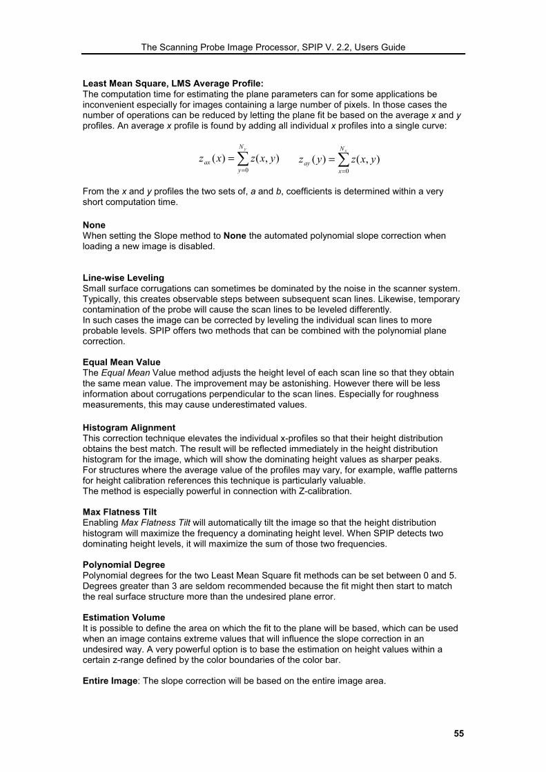
Least Mean Square, LMS Average Profile: The computation time for estimating the plane parameters can for some applications be inconvenient especially for images containing a large number of pixels. In those cases the number of operations can be reduced by letting the plane fit be based on the average x and y profiles. An average x profile is found by adding all individual x profiles into a single curve:
�=
=yN
yax yxzxz
0
),()(
�=
=xN
xay yxzyz
0
),()(
From the x and y profiles the two sets of, a and b, coefficients is determined within a very short computation time. None When setting the Slope method to None the automated polynomial slope correction when loading a new image is disabled. Line-wise Leveling Small surface corrugations can sometimes be dominated by the noise in the scanner system. Typically, this creates observable steps between subsequent scan lines. Likewise, temporary contamination of the probe will cause the scan lines to be leveled differently. In such cases the image can be corrected by leveling the individual scan lines to more probable levels. SPIP offers two methods that can be combined with the polynomial plane correction. Equal Mean Value The Equal Mean Value method adjusts the height level of each scan line so that they obtain the same mean value. The improvement may be astonishing. However there will be less information about corrugations perpendicular to the scan lines. Especially for roughness measurements, this may cause underestimated values. Histogram Alignment This correction technique elevates the individual x-profiles so that their height distribution obtains the best match. The result will be reflected immediately in the height distribution histogram for the image, which will show the dominating height values as sharper peaks. For structures where the average value of the profiles may vary, for example, waffle patterns for height calibration references this technique is particularly valuable. The method is especially powerful in connection with Z-calibration. Max Flatness Tilt Enabling Max Flatness Tilt will automatically tilt the image so that the height distribution histogram will maximize the frequency a dominating height level. When SPIP detects two dominating height levels, it will maximize the sum of those two frequencies. Polynomial Degree Polynomial degrees for the two Least Mean Square fit methods can be set between 0 and 5. Degrees greater than 3 are seldom recommended because the fit might then start to match the real surface structure more than the undesired plane error. Estimation Volume It is possible to define the area on which the fit to the plane will be based, which can be used when an image contains extreme values that will influence the slope correction in an undesired way. A very powerful option is to base the estimation on height values within a certain z-range defined by the color boundaries of the color bar. Entire Image: The slope correction will be based on the entire image area.

The Scanning Probe Image Processor, SPIP V. 2.2, Users Guide
56
Inside Marked Area, The slope correction will only be based on the data within the area marked by the rectangular marker. Outside Marked Area, The slope correction will only be based on the data outside the area marked by the rectangular marker. Frame Region, The plane fit will be based only within the specified outer frame. This is particular useful when the center part of the image contains a dominating feature like, for example, an indentation that could cause are wrong estimation of the surface bearing plane. Frame Width, The frame width can be set between 1 and 30% of the image width. Inside Color Range, perform the estimation on the pixels having height values inside the upper and lower color limits of the color bar. This enables a plane correction without influence from outliers or asymmetric distribution of e.g. pits. As this options can be combined with the Estimation Area options described above it is possible to determine an estimation volume rather than just a estimation area or z-range. It is highly recommended to use this option for accurate step height measurements. Correct AOI Only, only the region inside the zoom box will be corrected, but the surrounding will be leveled by constant values so that no edges will appear. Interactive Tilt The plane of the image can be tilted manually by use of the arrows and the tilt step can be controlled by the Tilt Height number entered in nm. It is possible to monitor the effect on the histogram distribution and a profile simultaneously by having these windows open. Z Offset The plane correction menu offers three ways of setting the Z Offset: Set Mean To Zero This will level the image so that the mean value of the image is set to zero. Keep Mean This will level the image so that the mean value of the original image is preserved. Set Min To Zero This will level the image so that the min value of the image is set to zero. Bearing Height to Zero This will define the bearing height as the most dominant height value (based on a height distribution histogram) and level the image so that it is set to zero. The dominant height value is identical to the value in the height distribution histogram having the highest frequency. Show Difference When this option is on the difference between the image before and after correction image is shown. This image is identical to the correction image and describes exactly how the image was corrected. Apply When clicking on the Apply button the selected slope correction method will be applied on the Main Image. Note that the selected slope settings will be applied whenever a new image is opened. The result is immediately reflected in the profile curve and the histogram if open. Reload You can reload the original image and discard all previous corrections by the Reload button. The actual settings will be applied to the reloaded image. To see the raw image it is necessary to disable the slope correction methods.

The Scanning Probe Image Processor, SPIP V. 2.2, Users Guide
57
Apply When Loading When this check box is set the current settings will automatically be applied in the following order:
4. Polynomial plane correction 5. Line-wise leveling 6. Max Flatness Tilt
Set Default Press Set Default to define the slope correction settings that will be loaded when SPIP is started.

The Scanning Probe Image Processor, SPIP V. 2.2, Users Guide
58
Fourier Menu The Fourier Menu has powerful features for characterizing images and performing Fourier filtering. Fourier Peaks The left part of the Fourier Menu is dedicated to Fourier peak analysis. When the circle marker is on it is possible interactively to mark a Fourier peak of interest. Having Defines Peak 1 or Defines Peak 2 enabled, parameters associated with the highest Fourier pixel in the circle will be calculated and written in the Peak Parameters box. Having defined Peak 1 and Peak 2, the associated unit cell is calculated and the results written in the Unit Cell Vectors box The right part of the Fourier Menu contains buttons for automated unit cell detection, filtering, and change of contrast, inverse transform and calculation of alternative unit cells
Detection Options Using the detection options it is possible to define how SPIP will calculate the position of the Fourier peaks: Use data window: When this check box is set on a Hamming data window is multiplied to the image before the Fourier transforms is performed; this is also true for the Sub-pixel Fourier algorithm.

The Scanning Probe Image Processor, SPIP V. 2.2, Users Guide
59
The function of the data window is to lower border effects of the images, which can cause stripes in the Fourier images and hide some of the more interesting structures or influence the calculation of the peak positions. Fast peak detection: When this check box is set on, the Fourier Peaks are found at sub-pixel level by a parabolic fit. Otherwise the Sub-pixel Fourier algorithm finds the peak, this is a more accurate algorithm but much more computer intensive because a high number of Fourier calculations for Sub-pixel Fourier components has to be performed. Circle Function Off: When this checkbox is set on the Fourier peak detection will not be activated when marking circles in the Fourier images. However, the circle marker can still be used for defining areas of interest for, e.g., filtering. Define Peak 1: Having this check box set on the highest Fourier component inside the circle marker will be found when ever a new circle has been defined. The co-ordinates, the corresponding wavelength and the associated time frequency in Hz will be calculated. Furthermore, the unit cell will be calculated when Peak 2 has been defined as well. Define Peak 2: This check box works similarly to the Define Peak 1 check box. Subpixel Zoom: When checked a zoomed sub-pixel image of the peak will be calculated. This option can be useful for evaluating the sharpness of the peaks and the accuracy of the peak automated detection. X,Y Pixel Range: Defined in terms of normal Fourier pixels the size of the area, which will be zoomed. X,Y Sub-Pixels: Defines how many sub-pixels in each direction will be calculated. Marker positioning and size Use the following marker positioning and size options to define the behavior of the circle marker tool. Snap: When Snap is set on the circle will be automatically positioned with the Fourier peak at the center after releasing the mouse button. Fixed Radius: When this option is set on the circle will have a fixed radius given by the numeric field and the Center at Origin option will be set off. The position of the circle marker is defined by the mouse pointer and the snap option setting. Center at Origin: When this check box is set the drawn circle will always have the center at the origin (DC) and the Fixed Radius will be set off. You may use this function to perform low-pass, high-pass or band-pass filtering. To perform a low-pass filter mark the cutoff frequency by the circle marker and press Include Only Peak Parameters When a peak has been defined by the circle marker its X, Y co-ordinates will be written as the Fourier pixel co-ordinates and the Z values are written as amplitude values using the same units as the main image. Note, that the Z values will be influenced by, for example, the square root and the square functions. When the information on the scanning velocity is known the time frequency associated with the Fourier peak is calculated and shown in the Hz field. Use this feature as a diagnostic tool for characterizing noise and vibration problems. The spatial wavelength associated with the Fourier peak will be written in the WL fields. You may use this function to determine repeat distances of, for example, line structures. Unit Cell Vectors The spatial unit cell is characterized by two unit cell vectors a and b for which the co-ordinates are written in the corresponding fields. The unit of the parameters will be identical to

The Scanning Probe Image Processor, SPIP V. 2.2, Users Guide
60
the lateral unit of the spatial image. Also, the absolute length of the unit cell vectors and their angle are written. The result of the unit cell detection will also activate and update the Calibration and Unit Cell Results dialogue window where the correction factors are shown. Furthermore the unit cell results are written to *.cal files, which may be used by third party programs for statistical analysis. Note that the calibration results only have meaning when the reference data exists and are set correctly. Otherwise, the unit cell detection function is a powerful technique for accurate characterization of lattice structures. Target Structure SPIP can detect oblique unit cells (the generic description of unit cells) and parallel lines. The detection is started by pushing the Oblique Cell or the Parallel Lines button. If the detection is successful the numeric fields describing the unit cell are updated and the unit cell is drawn in the spatial image. For line structures the a vector parameters describe the repeat distance and orientation while the b vector is a perpendicular vector set to a size identical to the width of the image. This makes it possible to apply the oblique marker on line structures as well. For noisy images where SPIP may fail to detect the lattice structure the detection algorithm may be assisted by removal of certain Fourier components, or by changing the scaling of the amplitude values (does not require an inverse Fourier transformation). WYSIWYG filtering can also improve the results but requires an inverse filter operation. Filtering It is possible to filter and image by exclusion of certain Fourier components and performing an inverse Fourier transform. The Fourier components to be excluded are selected by the marker tools and removed by the Exclude AOI (Area Of Interest) or Include Only buttons. The exclusion is performed by setting the amplitude values of the amplitude spectrum to zero. Independent of the chosen scaling, Exclude AOI will exclude all components within the marked areas while Include Only will exclude the exterior of the marked areas. Low-pass filtering: To perform low-pass filtering select the circle marker, set the Circle Function to Off and set Center at Origin on. Mark a circle with a radius corresponding to the desired cutoff wavelength. The wavelength and amplitude corresponding to the mouse position, which determines the circle radius is shown at the lower right corner of the SPIP program window. Thus, move the mouse until you read the desired wavelength. Then press the Include Only button. For a noisy image where SPIP might fail to detect the unit cell correctly, the detection algorithm can be assisted by exclusion of Fourier components associated with noise. High-pass filtering: High-pass filtering is done in the same manner as low pass filtering but by clicking on the Exclude AOI button instead of Include Only Band-pass filtering: Band-pass filtering can be performed by low-pass filtering followed by a high-pass filtering. When comparing, for example, roughness data of images acquired at different sampling densities and scan ranges it can be necessary to band-pass filter first so that the frequency limits of the images are alike. Otherwise, the image with the largest scan range will typically show the largest roughness number (RMS). Filtering by the Color Editor: It is possible to use the Color Editor as a WYSIWYG (What You See Is What You Get) interface. By changing the amplitude value for the height value associated with the lower color limit (usually black) of the color bar it is possible to define a threshold value and set all Fourier components below this value to zero when clicking on the Inverse button. If the threshold value is set low it will mainly affect the white noise and you may regard the technique as a white noise filter. The scaling form can change the sensitivity of this function Scaling By the scaling functions the contrast of the Fourier image can be changed. The Square Root and Logarithm buttons will enhance the weaker Fourier components, while the Square and Exponential buttons will highlight the more dominant components even more. The buttons can be pressed multiple times and their effect removed by their inverse functions or by the

The Scanning Probe Image Processor, SPIP V. 2.2, Users Guide
61
Undo button. The actual scaling can have effect on the unit cell detection because only Fourier peaks having height values greater than 1/1000 of the maximum value will be accepted. Also, the scaling will determine the sensitivity of the WYSIWYG filtering by the Color Bar. Transformation The New Fourier button will calculate a new amplitude spectrum of the actual Main Image. The used algorithms do not require any specific pixel dimension, except that there shall be an even number of pixels on the x- and y-axes. For uneven number of pixels, SPIP will extend the image by an additional column or row. SPIP applies fast Fourier algorithms for all image sizes but the best performance is achieved when the number of pixels on the axes is a power of 2. The Inverse button is used for transforming the Fourier image into a spatial image after the spectrum has been edited. This will overwrite the actual Main Image. Alternative Unit Cells A lattice can be described by alternative unit cells, the one SPIP displays is one having the angles between the a and b vectors most close to 90 degrees. Sometimes it might be convenient to display the detected unit cell differently to highlight the correspondence with, for example, single molecules. For this purpose SPIP provides four buttons a=a+b, a=a-b, b=b+a and b=b-a for interactive calculation of alternative unit cells by vector addition and subtraction. The result is displayed by the oblique marker in the Main Image and in the a and b vector fields of the Fourier Menu simultaneously.

The Scanning Probe Image Processor, SPIP V. 2.2, Users Guide
62
1D Fourier Analysis The Fourier transform of a profile is calculated when right clicking on one of the Fourier functions in a profile window. The 1D Fourier window has strong tools for analyzing periodic structures and diagnosing noise or vibration problems. To achieve the highest accuracy it will be an anvantage to apply the Fourier X 16 (Requires the Calibration Module) function of the Profile context menu. The 1D Fourier window has its own context menu activated by the right mouse click:
Cursor On; When right clicking on Cursor On or pressing ‘C’ on the keyboard the number of cursor pairs will change between zero, 1 and 2 pairs. The cursors can be used to measure a periodic distance (pitch) by moving a cursor to the first harmonic peak. Then the corresponding wavelength is calculated and written in the text field of the window, see example below.
The MX/M1 fields are used for testing the harmonic numbers; SPIP automatically divides the wavelength of the different cursors with the wavelength of curser M1. In this example, M1 points to the first harmonic, i.e., the pitch, M2, M3 and M4 are pointing to the 2nd, 3rd and 4th harmonics respectively, which is confirmed by the M2/M1, M3/M1, and M4/M1 fields. The higher harmonics can be used for getting a statically estimate of the pitch by multiplying the

The Scanning Probe Image Processor, SPIP V. 2.2, Users Guide
63
wavelength values by their harmonic numbers. Put Cursors on Peaks (Requires the Calibration Module) Click this function and the four highest peaks will be detected and indicated by the cursors. When using this automated technique the peak positions will be calculated at sup-sample level by parabolic fits, so that the wavelength calculations shown in the graph will have a much higher accuracy. Auto Update Cursors on Peaks (Requires the Calibration Module) This option will cause the Peaks to be detected (at sub-sample level and indicated each time the Fourier transform changes. dB Scaling; The dB scaling can be used to enhance the weaker details of the Fourier transform. The maximum Fourier value will be set to 0 dB. Log Log Scaling When the profile window contains an amplitude spectrum the fractal dimension can be evaluated by the Log Log function. The fractal dimension is defined as 2.0 minus the estimated slope of the Log Log plot. The fractal dimension can also be calculated for all directions of an image as part of a roughness analysis. Freeze Axes; when performing comparisons it can be useful to keep the axis frozen. Like wise it can be an advantage to duplicate a window before entering new data. Display options; Further display options can be set in the Properties menu (double click):

The Scanning Probe Image Processor, SPIP V. 2.2, Users Guide
64

The Scanning Probe Image Processor, SPIP V. 2.2, Users Guide
65
Lateral Calibration and Unit Cell Detection The lateral calibration depends on images containing structures with known pitch dimensions. The procedure can be performed in one or more steps depending on the accuracy required.
The process is started by clicking on the key for fast XY-calibration, , or the key for the
most accurate XY-calibration . This will automatically give you the necessary information about the unit cell, and correction factors shown in the Unit Cell and Calibration Results Menu. And if you believe that your system is linear the procedure is finished. Otherwise you should continue with the fine linearity analysis.
In the top of the menu are written the data for the detected unit cell vectors. By clicking on Correct Unit Cell, the unit cell parameters will be corrected by the correction parameters shown at the bottom of the dialog. Therefore if the correction parameters are already know it is possible to correct the detected unit cell without correcting the entire image. It is often useful to rotate an image so that the unit cell or line structure is parallel to the axes, - this can be done automatically by clicking on the Align Image by Rotation, see more details about image rotation in the Rotation section. Reference Data: Below the unit cell data, you can enter the proper reference values for the reference unit cell, the length of the two unit cell vectors and their angle. The correction parameters can be calculated based on three unit cell forms: Quadratic, Hexagonal, Rectangular or the generic Oblique form.

The Scanning Probe Image Processor, SPIP V. 2.2, Users Guide
66
Save & Recall Reference Data The reference data can be saved into individual files and recalled again. Note that the reference files *.crp may also contain step height information, which is preserved when saving the lateral reference data. Correction Parameters: Click on the Apply button to get the corresponding correction factors calculated. The three correction parameters xc, yc, dx/dy are the necessary parameters for reconstructing an image with correct scaling and angles. They are described in detail in the Reference Guide Lateral Calibration by Quadratic Unit Cells. Save & Recall Correction Data The calculated correction parameters can be saved and recalled so that they can be applied to other images. The menu can be opened directly from the menu bar: Processing→→→→XY-Calibration or Unit Cell Detection→→→→Correction Menu To perform a correction by the calculated correction parameters or some entered parameters by you, click on Correct. If the correction parameters were the one calculated from the current image, you can check the correction:
A new calculation of the correction parameters should result in values close to neutral, i.e., xc =1, yc =1, and dx/dy = 0. The quality of the results from this Fourier-based unit cell detection depends on the linearity of the scanner. If the image has distortion from hysteresis or some other phenomenon that causes non-uniform sampling of the surface it is advisable to continue with the Lateral Linearity Calibration.

The Scanning Probe Image Processor, SPIP V. 2.2, Users Guide
67
Lateral Linearity Calibration SPIP has two methods for linearity analysis implemented the Coarse Hysteresis Correction method and the Fine Linearity Correction method. The Coarse Hysteresis Correction method
The first applies to images where the distortions are caused by hysteresis. A 2nd order polynomial model is used for describing the hysteresis and the model is tuned so that the Fourier peaks are maximized. You can try the method on the hyst.bcr file which came with SPIP (to get adequate result on this specific file a license for analyzing images larger than 128 x 128 pixels is required).
Open hyst.bcr.
You will find that the repeat distance for the features is highest on the upper left part and smallest on the lower right part. This is an effect of non-uniform scanning caused by hysteresis. The scanner has sampled at equal time intervals but the scanning speed was lower on the upper left part where the scan started than the lower right part.
Take a look on the Fourier image and you will see that the narrow peaks typical of calibration objects has broadened to rectangular forms:

The Scanning Probe Image Processor, SPIP V. 2.2, Users Guide
68
Click on the coarse linearity button and a new corrected image will be calculated:
Make a new Fourier image and you will see that the Fourier peaks associated with the real structure have been restored

The Scanning Probe Image Processor, SPIP V. 2.2, Users Guide
69
Fine Linearity Calibration.
The Fine Linearity Correction method is a very powerful tool for finding non-linearity even smaller than the size of a pixel. It is therefore the best method for checking the quality of high-end metrology systems. Example: If you continue the with the hysteresis corrected image calculated as shown above by a fine
linearity analysis you will get a new image with the unit cell indicated together with error vectors.

The Scanning Probe Image Processor, SPIP V. 2.2, Users Guide
70
The red error vectors are of relative size and mainly used for visualizing the error direction and relative magnitude; the black points are the (0,0) anker points of the vectors. You can
turn the unit cell and error vector indication off by the oblique marker tool ’ The absolute magnitude of the linearity errors are best found in the scatter diagrams or the Linearity Correction Dialog where you still find some residual error within +/- 1.5 pixels:

The Scanning Probe Image Processor, SPIP V. 2.2, Users Guide
71
Continue by pressing Correct followed by New Estimate and you will find that all errors are in the sub-pixel regime:
The linearity analysis relies on the definition of a template, which is a representative repetitive structure. The user can define the template with the rectangle marker tool. When no selection is made SPIP will just create one which can cover a unit cell. Selecting a large template will provide the most robust result but requires more computation time. Smaller templates can provide more information about the linearity close to the image borders.
When a template is selected, the associated toolbar button starts the fine linearity analysis. If the unit cell has not been found earlier it will automatically be calculated by the Fourier method first. Then SPIP finds from the cross correlation the sub-pixel positions of all structures similar to the template shown in the zoom window. It will compare the positions with those predicted from the unit cell data. The differences are described as linearity errors, which are further, minimized by tuning the unit cell (now in the spatial domain). The results are shown in the Linearity Correction Menu:
Consequently, we have quantified the non-linearity as well as the best-fit unit cell. Experiments have shown that this gives a better reproducibility than the faster Fourier method. However, the Fourier method is needed for getting a good initial estimate of the unit cell. The overall linearity error Mean Position Error is also shown in the Linearity Correction Menu and more detailed information is written into the *.linc file. Correction Model The correction parameters are based on a third-order polynomial model of the scanning

The Scanning Probe Image Processor, SPIP V. 2.2, Users Guide
72
system. They describe how to resample the image. A more detailed description of the parameters is found in the reference guide. It is possible to enter your own values. Correct You can apply the correction parameters on the main image by clicking on the Correct button. New Estimate Recheck the linearity by clicking on New Estimate and you should observe that the correction parameters become more neutral, that the errors in the scatter diagram reduces to the sub-pixel level and that the Mean Position Error decreases. New Est, Keep Unit Cell When clicking on this button you will get a new estimation as above but without changing the current unit cell parameters. This gives you the possibility to see how sensitive the linearity analysis is to correct estimation of the unit cell. Unit Cell The unit cell co-ordinates are found from a least error fit, except when the New Est, Keep Unit Cell button is used. In this case you may enter your own co-ordinates and observe how sensitive the analysis is to the unit cell co-ordinates. Mean Position Error The mean position error measure the combined X and Y dislocations. Regard also this as a quality measure for the combined
1.Linearity of the instrument 1. Uniformity of the surface structure 2. Accuracy of the image processing.
Save & Recall The calculated correction parameters can be stored and retrieved. To apply the correction parameters to a different image you can active this menu directly from the menu bar: select Processing→Linearity→Correction Menu
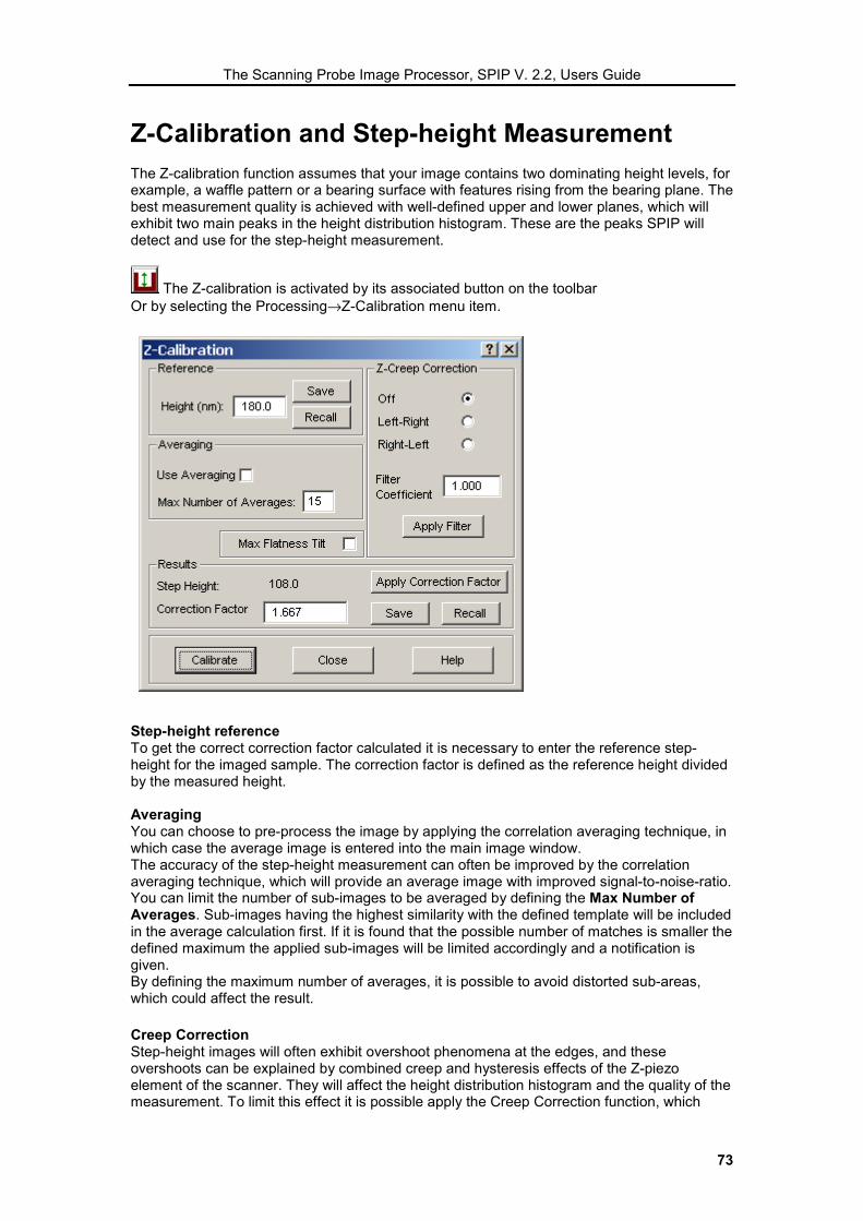
The Scanning Probe Image Processor, SPIP V. 2.2, Users Guide
73
Z-Calibration and Step-height Measurement The Z-calibration function assumes that your image contains two dominating height levels, for example, a waffle pattern or a bearing surface with features rising from the bearing plane. The best measurement quality is achieved with well-defined upper and lower planes, which will exhibit two main peaks in the height distribution histogram. These are the peaks SPIP will detect and use for the step-height measurement.
The Z-calibration is activated by its associated button on the toolbar Or by selecting the Processing→Z-Calibration menu item.
Step-height reference To get the correct correction factor calculated it is necessary to enter the reference step-height for the imaged sample. The correction factor is defined as the reference height divided by the measured height. Averaging You can choose to pre-process the image by applying the correlation averaging technique, in which case the average image is entered into the main image window. The accuracy of the step-height measurement can often be improved by the correlation averaging technique, which will provide an average image with improved signal-to-noise-ratio. You can limit the number of sub-images to be averaged by defining the Max Number of Averages. Sub-images having the highest similarity with the defined template will be included in the average calculation first. If it is found that the possible number of matches is smaller the defined maximum the applied sub-images will be limited accordingly and a notification is given. By defining the maximum number of averages, it is possible to avoid distorted sub-areas, which could affect the result. Creep Correction Step-height images will often exhibit overshoot phenomena at the edges, and these overshoots can be explained by combined creep and hysteresis effects of the Z-piezo element of the scanner. They will affect the height distribution histogram and the quality of the measurement. To limit this effect it is possible apply the Creep Correction function, which

The Scanning Probe Image Processor, SPIP V. 2.2, Users Guide
74
adaptively finds the first-order low-pass filter that results in the best histogram, i.e., the one with the highest peaks for the upper and lower planes. Note, that the found filter usually only will have little effect on other parts of the image. This is because a filter that changes too much will also destroy the slopes and thereby flatten the histogram, which is exactly not desired. If averaging has been selected this correction will be applied only to the average image. The filter has the following form and it is the a parameter that is estimated:
1x )1(z −−+= xx zaaz Because creep depends strongly on the scanning direction, it is necessary to enter the original scanning direction. The filter coefficient found will be displayed and it is possible to enter other filter coefficients and apply them to any image.
Max Flatness Tilt When setting Max Flatness Tilt On, the image will be tilted (first-order plane corrected) by an iterative procedure so that the histogram peaks are maximized. When the averaging option is set, the max flatness correction is applied to the average image.
Activation The Calibrate button or the Enter key activates the selected calibration procedure. Results The results are indicated in the menu and in the height distribution histogram:
The Z-height values associated with the two histogram peaks are indicated at the peaks. The difference between the peaks reflects the Step-height, which is written at the upper left part of the histogram and the calculated correction factor is written below. At the very top is the total Z range for the image written. To keep track of the calibration history the result is also written to a file with extension .zcal which is a simple text file that can be imported to a spreadsheet program.
The Z-Calibration result can be checked by applying the Z-correction factor and perform a new calibration. You can also enter you own correction factor and apply it to any image.

The Scanning Probe Image Processor, SPIP V. 2.2, Users Guide
75
Correlation Averaging Correlation averaging is a powerful tool for analyzing images containing repeated structures like atoms, molecules or calibration patterns. The technique can find all the repeated structures and add them so that an average image of the recurrent structure is obtained. In ideal situations the signal-to-noise-ratio can be improved by the square root of the number of additions. In contrast to other filtering techniques it will not filter specific frequencies but preserve all frequencies that are represented in the repeated structure. The following example is based on an STM image of Didodecyl-benzene molecules selfassembled on a graphite substrate.
Pressing the associated key starts the correlation averaging. If the zoom image is active SPIP will use this image as the structure that has to be recognized and averaged, otherwise SPIP automatically determines a suitable template based on unit cell detection. Let us
assume you define the template by the rectangle marker tool :
The template will also be seen in the zoom window:
Start the correlation averaging by the toolkey or from the meny: Processing→→→→Average→→→→Marked Area, Correlation Averaging.

The Scanning Probe Image Processor, SPIP V. 2.2, Users Guide
76
The process will create a cross correlation image displaying peaks associated with the individual areas matching the template. From the cross correlation peaks and the raw image the Average image together with the Standard deviation image are calculated. The latter will contains detailed information about the uniformity of the structures and noise in the instrument. Also, the standard deviation image may provide important information about structural uniformity, and for example reveal details on how self-assembled molecules are attached to a substrate. The SD Image shown below displays low SD values at the right part of the benzene rings indicating that this part of the molecule is the part most fixed to the substrate.

The Scanning Probe Image Processor, SPIP V. 2.2, Users Guide
77
Rotation It is often useful to have structures of an image oriented so that they are parallel to the axes. SPIP provides three ways to rotate and image: 1) by a user defined angle value 2) by an angle defined by the line marker 3) automatically based on a calculation of the unit cell or line structure. The rotation dialog is activated by a right click in an image window or from the Processing pull down menu, and the procedure can also be part of a batch process.
The Align Unit Cell is only available if the unit cell or line structure has been calculated first. If so it can automatically perform a rotation as shown below and the optional average profile calculated as well:

The Scanning Probe Image Processor, SPIP V. 2.2, Users Guide
78
The rotation angle can also be defined by a marked line or by an absolute value. The absolute rotation angle can be changed interactively by the up-down keys while observing the result simultaneously. The average profile of the resulting rotation image can be shown automatically by setting the Show Average Profile check box. The averaging is done so that the void areas are not included in the calculation and provides the best possible estimate of the average profile. See also the above example.

The Scanning Probe Image Processor, SPIP V. 2.2, Users Guide
79
Roughness
Start the roughness calculation by the key symbolizing the bearing curve. The roughness analysis will then be based on the Main Image. It is also possible to calculate roughness parameters from profiles by Right Clicking in the Curve Window. For Images a set of 20 roughness parameters can be calculated and depending on the options defined in the Options Dialog the results may written to files with the added extension .rgh or to the database of the ImageMet Explorer. For profiles a subset of 14 parameters are calculated. Roughness parameters based on Image will have the prefix ‘S’ and when based on a profile the prefix ‘R’ is used. For example will the Roughness Average Parameter be denoted Sa and Ra for images and profiles respectively. The result file will automatically be shown in the Notepad program:
For convenience, the data is written in both a row and a column form. Depending on how you want to organize the data in a spreadsheet, you can ignore one of the two forms. The files can be used for statistical analysis by third party programs. A definition of the different roughness parameters is found in the Reference Guide, Roughness Parameters. The roughness analysis will also generate the bearing curve (Abbott). In the case that the Fourier Image has been calculated the Angular Spectrum, the Radial Spectrum, the Integrated Radial Spectrum and the Fractal Dimension windows are shown too. The angular spectrum and the fractal dimension are shown in Polar Plots (also called Rose Plots) with a value for all discrete angles between 0 and 180 degree. The parameters depending on the Fourier image are only calculated when the Fourier image is exists. The fractal dimension is calculated for the different angles by analyzing the Fourier amplitude spectrum; for different angles the Fourier profile is extracted and the logarithm of the

The Scanning Probe Image Processor, SPIP V. 2.2, Users Guide
80
frequency and amplitude coordinates calculated. The fractal dimension for each direction is then calculated as 2.0 minus the slope of the log - log curves. The fractal dimension can also be evaluated from 2D Fourier spectra by application of the Log Log function. If the surface is fractal the Log Log graph should be highly linear.

The Scanning Probe Image Processor, SPIP V. 2.2, Users Guide
81
Grain Analysis The Grain Analysis Menu is used for quantification of grains/particles and pores/pits.
The menu is activated by the corresponding toolbar button or by selecting Processing→→→→Grain Analysis in the Main Menu.
Contrast Enhancement The results can sometimes be improved by enhancing the contrast. The Grain Analysis Menu offers two ways to enhance the contrast, by Local Mean equalization and by Local Standard Deviation equalization. The first method simply subtracts the mean value of the nearest neighbor pixels within the filter window. The SD equalization scales the height values by a factor given by the SD of the global image divided by the local standard deviation found in the filter window. To see the calculated local mean or local SD images used to enhance the contrast set the Show options on. The filter window, i.e., the number of pixels used for calculation of the local mean and SD values is defined by the X, Y Filter Size parameters.
Mode

The Scanning Probe Image Processor, SPIP V. 2.2, Users Guide
82
The mod defines whether it is grains or pores that is detected. In the Grains mode only the pixels having height values above the detection level is considered while it is opposite for the Pore mode. Detection Level The detection level defines the minimum height for a pixel to be regarded as part of a grain / particle. The Detection level works in correspondence with the Color Scale Editor, where the Lower Color Limit of the color bar reflects the detection level. This way you will get a direct visual feedback from the colors in the Main Image. Colors differing from the minimum color (usually black) will enter the analysis. By moving the lower color limit in the color bar the Detection Level of the Grain Analysis Bar will change simultaneously. It is recommended to use the
High Contrast color scale
Minimum width Particles smaller than the entered minimum width will be rejected unless the Ignore checkbox is set.
Maximum length When particles are found to be longer than the maximum length, SPIP will regard the object as overlapping particles and will search for an obvious cutting path. If no obvious cutting path is found the particle will not be split. The algorithm is iterative so that the two new particles created by a separation might be split once more.
Cut at Local Minimum. Grains that are close together can sometimes be hard to separate when the background amplitude is above the threshold level. In such situations it will help to set the Cut at Local Minimum option On. This has the effect that the local minima pixels will be regarded as pixels below the threshold level. For images with noise this option may cause too many separations and falls detection. Results The results are visualized in the Grain Image and depending on the options defined in the

The Scanning Probe Image Processor, SPIP V. 2.2, Users Guide
83
Options Dialog the results may written to text files with the added extension .grn or to the database of the ImageMet Explorer. The text file can easily be imported to a spreadsheet program. The result file can optionally be shown by the Windows NotePad program. Optional histograms showing the area and length distribution will be created and it is possible to set the number of elements in the histograms.
In the Grain Analysis Result dialog the results from the individual objects can be easily checked. The Grain/Pore ID’s can be entered or defined by clicking in one of the found objects in the Grain Image Window. It is possible to ignore the individual features from the calculation of the statistical results. In particularly it is possible to ignore all features at the borders, which may reduce the average results and increase the standard deviation in an undesired way. When an object is ignored its colors will turn into gray. Below is seen an example from a pore (pit) analysis of a waffle pattern.

The Scanning Probe Image Processor, SPIP V. 2.2, Users Guide
84
You can also determine the correspondence between the grains shown in the Grain Image Window and the data in the result file, because the Z-height in the Grain image is equal to the Grain ID written in the file: The Z-Height (i.e. the grain ID) is found by placing the mouse pointer over a grain and observing the (X, Y, Z) co-ordinates at the lower right of the program window. In the Property dialog of the image window you can set the coordinates to reflect the pixel position instead of the default physical coordinates.
Here the Grain ID is 97. Detect Grains The Detect Grains button activates the grain detection algorithm.

The Scanning Probe Image Processor, SPIP V. 2.2, Users Guide
85
Tip Characterization The SPIP tip characterization module allows you to characterize the tip or stylus used for scanning the actual image. The basic methods used are very similar to the blind reconstruction method described by J. S. Villarrubia and P. M. Williams et. al.
The tip characterization can run on all 2D images and is activated by its tool key or the Tip Characterize menu item found in the right mouse menu or the Processing sub-menu. If you have the Batch Processing option included in the software you can also run the tip characterization and Deconvolution in a batch process and combine it with other functions and thereby improve your productivity. There is four tip processing functions available for batch processing: Tip Deconvolute, Tip Characterize, Tip Load and Report Tip Characterization to HTML. Likewise, it is possible to combine the Correlation Averaging on repeatable structures and thereby minimize the influence from noise.
In the Tip Characterization menu different detection parameters influencing the result can be set. It is important to notice that if we can assume that there are no image distortions, apart from tip artifacts, SPIP will be able to calculate the worst case tip. The worst-case found tip is able to scan all parts of the surface with its apex but might be sharper in reality. Detection Options Size The Size parameters defines the number of pixels for the tip to be estimated, uneven numbers in the range 3 to 99 are possible; this way the tip apex will always be centered. The tip size can not exceed half of the surface image size. Iterations The Iteration number determines how many times the recursive algorithm will run through the image. First time the tip is evaluated only from the true maximums. Based on this tip we can create the Certainty Map by emulating a tip scan. This image tells us which part of the image that is scanned by the apex and can be trusted. In the second iteration all local maximums in the trusted image areas are used for further tip estimation and a new Certainty Map is

The Scanning Probe Image Processor, SPIP V. 2.2, Users Guide
86
created. Third and higher numbers of iterations are similar to the 2nd but now all trusted pixels are included. The computing time depends linearly with the number of iterations and it will seldom be necessary to use more than 3 iterations. Trust Trust pixel area defines how many pixels are trusted in 2nd and following iterations. When estimating a large area of a tip the uncertainty of the border points will be much lower that the center pixels and can reduce the Certainty surface area because it will be difficult for the tip to enter the lower surface levels. This means that there will be fewer places where tip shape information can be deduced resulting in a too blond tip. If this is a problem it can be an advantage to define the Trust pixel area to be smaller than the tip area meaning that we are ignoring the tip outer parts when calculating the certainty area. In most cases you should keep the Trust area equal to the tip size but especially when performing the characterization on pores rather than particles this option can be useful. Reduce Spikes Depending on the image quality the tip characterization result may be influenced by noise and this is especially true when there are noise peaks creating maximums that are going to be used by the first iterations of the characterization algorithm. In these cases it is therefore important to have an intelligent way to reduce noise peaks. When Reduce Spikes is option is set, the tip is pre-calculated using only the first iteration described above. From the x and y profile of the tip the slopes at the very apex are evaluated. If the slopes at the very apex is higher than the slopes just below this is regarded as a noise artifact and the height at the tip apex is then lowered so that the slopes at the apex does not exceed the slopes just below. Using the knowledge of the noise reduced tip we are now able to detect all parts of the image where we have peaks sharper than the tip and then reduce these values so that they in the following iterations doesn’t causes the sharpness of the tip to be overestimated. Note, that the input image will be changed by this procedure but you can regard the technique as an intelligent way of detecting and removing noisy peaks. Acceptance Level If there is noise in the image, especially spikes, the sharpness of the tip can easily be over estimated. In such cases it is a good idea to increase the tip detection count, which is the number of occurrences in the image that a certain part of the tip would be inside the surface. This can of course not be true but is a way of ignoring the spikiest parts of the image. After the tip has been characterized you can set the detection count interactively by the scroll bar and in real-time observe how it changes the estimated tip. Note, that the Acceptance level will influence the Certainty Map and thereby alter the tip estimation after 1st iteration in the tip estimation algorithm. Characterize When pressing the Characterize button the tip characterization will be started and it will be based on the image window for which the tip characterization was invoked the first time. Below is seen a screen dump after a tip characterization with the estimated tip seen in top view and 3D perspective. The gray image is the Certainty Map and is the result of a tip scan emulation by the estimated tip and the surface image. The red marks indicate the positions where the tip is probing the surface with other parts than its apex. Also the tip x- and y-profiles are shown with their estimated tip radius (based on a circle fit) and the cone angles (based on the three center points) written. The following image is an AFM image of an evaporated gold film; kindly provided by the Danish Institute of Fundamental Metrology and demonstrates a blind reconstruction of the AFM tip.

The Scanning Probe Image Processor, SPIP V. 2.2, Users Guide
87
Load Tip After having estimated a tip you can save it in the BCR format, load it again and use it for Deconvolution of other images. Note, that only tips saved in BCR format can be loaded. If you have a tip in another format you may be able to use SPIP to convert the tip image to BCR format. If the resolution (physical distance between pixels) of the loaded tip is different from the image to be de-convoluted the tip will be resampled to obtain the same resolution and a message will be given. Emulate Scan By the Emulate Scan push button it is possible to scan the Main Image with the current tip shown in the Tip Top View window, this process is also called dilation. The resulting image is called the Certainty Map because areas un-touched by the tip apex are detected and marked with the red color. It is possible to use this function on artificial tips and surfaces and learn how different tips can affect the observed images and the quantitative results. ’Deconvolute’ Deconvolution is important for correct line width measurements and can also assure more accurate results in particle size analysis and roughness measurements.

The Scanning Probe Image Processor, SPIP V. 2.2, Users Guide
88
Pressing the Deconvolute button will calculate a new image based on the Main Image and the actual tip shown in the Tip Top View window, this technique is also known as erosion. The process has only meaning when the surface structure has sharper edges than the tip. In such cases it is partly possible to correct for the width of the tip, which otherwise causes line width and the lateral size of particles to be overestimated. Results A number of quantitative results can be extracted from at tip characterization process, which can be reported in html when using batch processing Tip Radius: is determined by a sphere fit to the estimated tip. Small radii characterize quality tips. The Radius is calculated from a sphere fit to the 5x5 center pixels of tip. Certainty Area: is the percentage of the surface that could be probed by the tip apex. If this number is low you could consider exchanging the tip with at sharper one. Profiles: it is optional to view the tip x and y-profiles; if they are on they will also display the profile radii based on circle fits to the 5 center points. The fitted circles can be visualized by setting Show Fitted Curve On. Likewise, they will show the Tip Cone Angles, which are calculated based on the three center points. Saving the numerical results Depending on the options defined in the Options Dialog the numerical results may written to files with the added extension .tip or to the database of the ImageMet Explorer View Tip in 3D If you have the 3D Visualization Studio included in the software you can automatically visualize the tip in 3D. Confidence Graphs It is possible to display how the different quantitative results depends on the Detection Count Setting: Tip Radius, Tip Height (Height range of estimated tip), and X,Y Cone Angles. This may help you to optimize the Detection Count selection and estimate a tip based on a compromise between small noise influence and high utilization of the image information.

The Scanning Probe Image Processor, SPIP V. 2.2, Users Guide
89
Force Curve Analysis The force curve analysis menu is activated either automatically when opening a file with force curve data or selecting the menu item Force Curve Analysis in the right mouse key menu of a curve window or the curve menu of the menu bar.
The menu enables the creation of new graphs where force and separation are calculated based on the spring constant and the deflection signal as function of the height. The cantilever sensitivity (V/nm) can be calculated automatically from the slope of the extending (blue curve) or retracting curve (red curve) where the repulsive forces are dominating. The deflection measured in nm is calculated by dividing the deflection voltage with the cantilever sensitivity and the separation between sample and cantilever can be calculated from the sum of deflection and the height signal (where low height values means that the sample is close to the sample). SPIP will set the found minimum separation to zero. The Force values are calculated from the product of the cantilever spring constant (nN/nm) and the calculated deflection [nm]. Sometimes it might be most convenient to show the attractive forces as positive and the repulsive forces as negative forces, e.g., when analyzing curves from unfolding protein experiments. This can be set by the Set Attractive Forces Positive check box.
It is possible to enter a spring constant or let SPIP read it from the file if it is included. The cantilever sensitivity can be calculated automatically or entered manually. In the latter case the sensitivity can be evaluated from by use of the cursors. Setting two cursors on one of the curves in the engage region will cause the slope dy/dx corresponding to the cantilever sensitivity to be calculated. There is a cursor pair available for each curve (extending and retracting) see below.

The Scanning Probe Image Processor, SPIP V. 2.2, Users Guide
90
In this case the calculated Force (Separation) graph looks as below, although the x-coordinates are non-equidistant spaced it is possible to activate the cursors and perform measurements as on normal curves.
When Fit Worm Like Chain Model (WLC Model) is checked a WLC model will automatically be calculated from each detected unfolding event. The model is based on the following formula:
��
���
�−++
−=
41
)/1(41)( 2 Lc
xLcxl
TKxFp
B
Where F(x) describes the Force as function of separation x, KB is the Boltzmann’s constant, T the temperature in Kelvin, lp the persistence length and Lc the Contour Length, which is presented as the result in the graph. It is also possible to force a WLC fit to a certain part of the curve defined by the zoom box for this purpose right click in the Force Separation Graph on Force WLC Fit Inside Zoom. When more than two unfolding events is detected the individual Contour Length results will be displayed as function of the event index. The slope of this graph is automatically calculated and reflects the domain contour length in the protein. Below is seen an example of a Worm Like Chain Model analysis, the upper graph is the raw curve, below is a Base Line Corrected version and then the Force(Separation) graph with two fitted WLC models is shown with a zoom at the bottom. Data Courtesy of Michael Wrang Mortensen, Danish Institute of Fundamental Metrology.

The Scanning Probe Image Processor, SPIP V. 2.2, Users Guide
91
Detect Pull-Off Force Enables the calculation of the pull-off force on the retraction curve, which will be shown in the Force(Separation) graph. When Base Line Correct is set on SPIP will automatically fit a 3rd order baseline to the approach curve (Ignoring the contact regime). This base line is then subtracted from the approaching curve as well as the retraction curve. The base line estimation region can also be defined manually by the zoom box, it will then be processed by a right click in the Deflection(Z) curve window on Base Line Correct Within Zoom.

The Scanning Probe Image Processor, SPIP V. 2.2, Users Guide
92
Hysteresis Correct; This option will cause SPIP to shift the retracting curve so that it will overlap with the extending curve in the contact region. When the Apply button is pressed the requested curves are calculated and shown but in contrast to when the OK button is pressed the Force Curve Menu stays active. The entered settings can be saved to Force Curve Settings (*.fcs) files and defined as default by saving the settings to the file called Default.fcs. Average: To perform force curve averaging of multiple force curves all the curves of interest should be loaded into the SPIP program first. Then, when pressing Average SPIP will find all force curves of same type as the active force curve connected to the dialog and perform the average calculation. Curves of size or type different from the active force curve will automatically be ignored. The quality of the result depends strongly on the alignment of the curves and the program will prompt you for selecting one of two alignment methods. The first is based on an alignment of the minimum curve values, which typically is related to the pull-off point. The second method performs the alignment by minimizing the mean square sum difference. After averaging you can turn the average curve into the active force curve by right clicking in it is window on Force Curve Analysis.
The Scanning Probe Image Processor, SPIP V. 2.2, Users Guide
93
Continuous Imaging Tunneling Spectroscopy The Continuous Imaging Tunneling Spectroscopy (CITS) module allows you to visualize and handle I/V spectroscopy data. The availability of this function depends on the file format used by the STM vendor. If your file format is not supported please contact us for an upgrade. When opening a file SPIP checks if there is CITS data included in which case it will display three windows:
1) The topographic window with a grid overlay indicating the positions where the I/V spectroscopy data was acquired. When clicking on this grid the I/V curve acquired nearest to the associated mouse position will be displayed in a curve window. The curve window will indicate the (row, column) coordinate identifying the origin of the I/V curve. To show more graphs simultaneously as demonstrated in the screen example below the I/V curve windows can be duplicated (CTRL+-D). It is a good idea to press the SHIFT key while clicking with the mouse to prevent Double click events that starts the Image Property Dialog.
2) The CITS Volume Image, where the current is shown for a selected voltage. This window contains also a grid indicating the positions of the individual I/V acquisitions and the individual I/V curves can be selected the same way as for the topographic window. In addition to this it is possible to select the Voltage for which the current will be shown. This is done by a CTRL Mouse key combination; when keeping the mouse pressed together with the CTRL key and moving the mouse upwards the voltage will increase.
3) A spectroscopy image where each horizontal line represents an I/V Curve. The lines are ordered by the acquisition time with the first curve shown in the upper line.
The CITS Volume and the Spectroscopy images can be transformed into conductivity (dI/dV) data, or the Density of States (dI/dV * V/I) using the right mouse menu. The CITS data shown below is kindly provided by Abdou Hasssanien, Electrotechnical Laboratory, Tsukuba,Ibaraki, http://www.etl.go.jp/
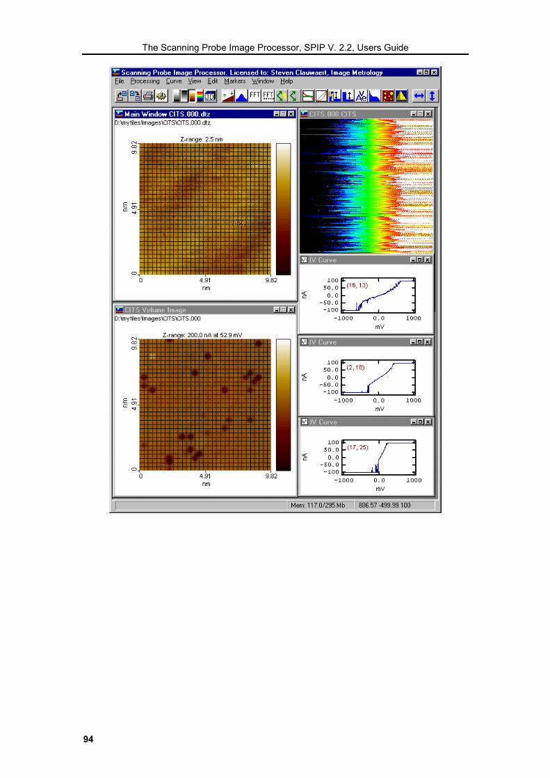
The Scanning Probe Image Processor, SPIP V. 2.2, Users Guide
94
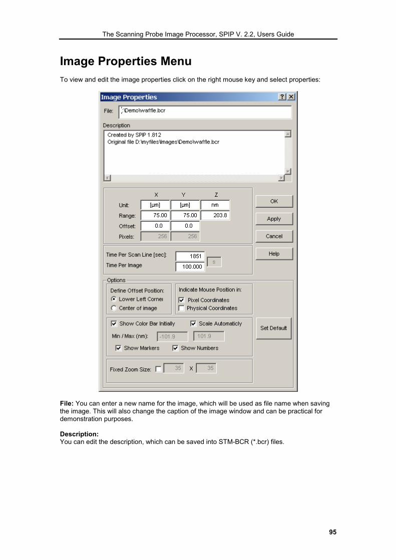
The Scanning Probe Image Processor, SPIP V. 2.2, Users Guide
95
Image Properties Menu To view and edit the image properties click on the right mouse key and select properties:
File: You can enter a new name for the image, which will be used as file name when saving the image. This will also change the caption of the image window and can be practical for demonstration purposes. Description: You can edit the description, which can be saved into STM-BCR (*.bcr) files.

The Scanning Probe Image Processor, SPIP V. 2.2, Users Guide
96
Units: The units for the three axes can be defined, but the numerical values will stay unchanged. Depending on the range of the different dimension SPIP might show length using the most appropriate units. Currently SPIP recognizes the following length unit abbreviations:
• Å, A: Ångstrøm • nm, nanometer • µm, um, micrometer • mm, millimeter • cm, centimeter • in, inch • m, meter • km, kilometer
The units are also recognized when included in brackets, e.g., [um] Range: The range can be changed for all three dimensions. This is in particularly useful for graphical formats like tiff, bitmap and jpeg where the physical size of the image area is not included in the file. When changing the Z-range the Z-values will be scaled so that the difference between the maximum and minimum values equals the entered Z-range. Offset: The offset parameters describes the physical position of the image area relative to the scanner / acquisition instrument. Timing Information The timing information defines how fast the image area was scanned (and has only meaning for scanned images). These parameters are important for correct calculation of time domain frequencies when diagnosing noise and vibration problems using the Fourier Menu. Options There are several options, which will determine how the current image will appear and can be set at defaults. Define Offset Position The offset position can be associated with the center of the image or the lower left corner. Mouse Position Information When the mouse cursor is located in an image window its position relative to the image coordinates are written in the lower right corner of the program window. These coordinates can be expressed in pixels or in physical dimensions. Color Scale The color scale can set to cover the full z-scale of the image automatically or to cover a fixed range. The latter can be useful for comparing images. Here, you can also define if you want to have the color bar shown by default when saving this parameter as default it will only apply to images of same class, i.e., Main Image, Fourier Image and others. Fixed Zoom Size When zooming using the rectangular marker tool it can often be convenient to have a zoom box of a certain size. The numbers entered will be in terms of pixels of the raw image and work independently of the actual window size. Set Default When pressing Set Default all parameters defined in the Options frame will be saved along with the associated image class: Topographic image or Fourier Image. For the Show Color Bar Initially SPIP will also distinguish between the Main Image Window and other topographic image window, thereby you can have the Main Image to appear differently from the other topographic images.

The Scanning Probe Image Processor, SPIP V. 2.2, Users Guide
97
Batch Processing and HTML Reporting The batch-processing menu enables you to design your own processing sequence for each file opened. A group of files can be drag dropped from windows explorer or selected from the Open File Menu.
The menu is activated by the corresponding tool key or from Processing����Batch Processing.
The processing sequence can be selected from the left list box by double clicking or by the Add>> button. In the information box below there will be written a short description of the selected function. The sequence order can be changed by the up/ down arrows; the top most command will be processed first. To save memory it is a good idea to delete the current windows whenever a new file is loaded; this is set by the Delete Windows Before New Loading check box. Setting the checkbox Run when loading files will cause the sequence to be performed when loading a new file or group of files but only when the batch dialog is open. Reporting to an HTML file can be carried out automatically if the HTML Report checkbox is set. You may define the HTML file name or let SPIP define a name based on the current date and time of day, in this case the file will be located in the SPIP/HTML directory. During the batch processing screen dumps can be saved in JPEG files, which will be saved in the same directory as the HTML report file or to the directory of the Main Image file in the situation where HTML reporting is disabled. Numerical results can be saved together with the screen dumps by including Report Calibration to HTML or Report Calibration to HTML. This will also enable a statistical reporting of mean and standard deviation report for the file sequence at the end of the HTML report. The sequence example shown above will produce a HTML report with calculation of roughness parameters and a screen dump for each file in the sequence and will finally enter statistical results at the end of the HTML report. Note that during the batch process current defined reference parameters for calibration and slope correction and 3D visualization will be applied. You can in the corresponding menus store your preferences as the default settings, which will be loaded at program start.

The Scanning Probe Image Processor, SPIP V. 2.2, Users Guide
98
The different analytical operations available in the Batch Processing menu applies mainly to the Main Image Window, but it is possible to put the image from the most recent generated window for example a gradient images into the Main Window and then process with all the optional batch operations. The Store / Recall buttons allows you to save and retrieve the designed sequences. A default processing sequence can be defined by storing into the settings into the Default.batch file. SPIP comes with a number of sample files, which can be recalled from the Settings menu. When running the information box will inform about the status of the batch process. Currently a logo for the report can be included in the HTML report by having the logo in a file called Logo.gif this file should be located in the same directory as the HTML file. Similarly operator information can be included in the header by writing this information into a plain text file called Operator.txt.

The Scanning Probe Image Processor, SPIP V. 2.2, Users Guide
99
Multiple Image Analysis It is possible to have several images open at the same time and you can use the Right Mouse Key Menu to Duplicate, Exchange with the Main Image or Send to the Main Image for a more detailed analysis:
It is also possible to analyze differences of very similar images by subtracting an image from the Main Image. Before subtraction it can be an advantage to align the images by Align To Main, which will shift the current image in the x-y plane to give the best match defined by the cross correlation function. When having more images of same size open it is possible to create profile at the exact same positions using the Synchronized Multi Profiling tool. To open a group of files you can Drag Drop group of files or even entire folder branches from ImageMet Explorer or the MS Windows Explorer.
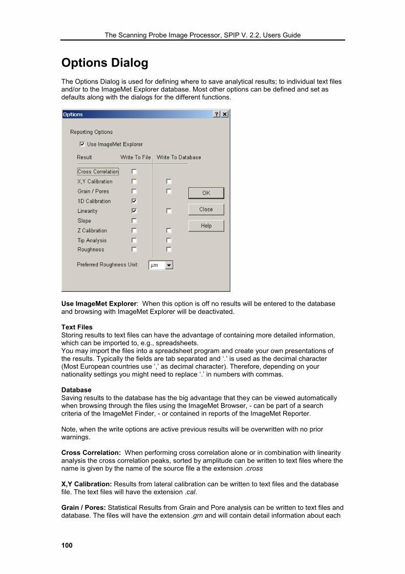
The Scanning Probe Image Processor, SPIP V. 2.2, Users Guide
100
Options Dialog The Options Dialog is used for defining where to save analytical results; to individual text files and/or to the ImageMet Explorer database. Most other options can be defined and set as defaults along with the dialogs for the different functions.
Use ImageMet Explorer: When this option is off no results will be entered to the database and browsing with ImageMet Explorer will be deactivated. Text Files Storing results to text files can have the advantage of containing more detailed information, which can be imported to, e.g., spreadsheets. You may import the files into a spreadsheet program and create your own presentations of the results. Typically the fields are tab separated and ‘.’ is used as the decimal character (Most European countries use ‘,’ as decimal character). Therefore, depending on your nationality settings you might need to replace ‘.’ in numbers with commas. Database Saving results to the database has the big advantage that they can be viewed automatically when browsing through the files using the ImageMet Browser, - can be part of a search criteria of the ImageMet Finder, - or contained in reports of the ImageMet Reporter. Note, when the write options are active previous results will be overwritten with no prior warnings. Cross Correlation: When performing cross correlation alone or in combination with linearity analysis the cross correlation peaks, sorted by amplitude can be written to text files where the name is given by the name of the source file a the extension .cross X,Y Calibration: Results from lateral calibration can be written to text files and the database file. The text files will have the extension .cal. Grain / Pores: Statistical Results from Grain and Pore analysis can be written to text files and database. The files will have the extension .grn and will contain detail information about each

The Scanning Probe Image Processor, SPIP V. 2.2, Users Guide
101
particle/pore. 1D Calibration: Results from a 1D Calibratoin (parallel lines) analysis can be stored to text files with the extension .lin Linearity: Linearity analysis results consisting of error description as well as correction parameters can be written to text files and database. The text files will have extension .lin Roughness: Roughness parameters can be written to text files and database. The text files will have extension .rgh Slope: Slope correction parameters used for correcting the image plane can be stored in text files with extension .slope Z Calibration: Z-calibration results can be saved in text files and the database. The text files will have the extension .zcal Tip Analysis: Tip analysis results can be saved in text files and the database. The text files will have the extension .tip Preferred Roughness Unit: Although SPIP is handling all height values in nanometers you can define another unit for reports of roughness results.

The Scanning Probe Image Processor, SPIP V. 2.2, Users Guide
102
Reading of Unknown File Formats When trying to open a file that is not directly supported by SPIP, the Read a Special File Format Menu is activated. You have the option to let SPIP guess the structure or provide SPIP with some information about the format. This way you will be able to read almost any file excluding files containing compressed data. For accurate measurements, it is necessary to enter the correct physical scaling parameters.
File This field initially contains the name of the file, which format was not recognized by SPIP. By putting in a name for a file that is recognized you can force SPIP to read the file in a different way. This can be a temporary solution when your microscope vendor has changed the format, for example, included multiple images in the same file. If such a situation occur, please contact Image Metrology so that we can implement a proper solution. Data Type SPIP currently supports four binary word types in addition to ASCII. It is important that you enter the correct word type and if you are in doubt consult your microscope manual or just try the different possibilities. Most SPM file formats consist of a fixed-sized header describing the image followed by Nx × Ny 16 bit signed integers. You will usually be able to distinguish a correctly read image from a wrong. Intel Word Format The binary words are usually in the Intel format. However, if your data source is a UNIX or

The Scanning Probe Image Processor, SPIP V. 2.2, Users Guide
103
Macintosh workstation it is more likely that you need to turn off this setting. Structure Information Header Length The Header Length is the number of 8-bit bytes in front of the raw data. Number of X,Y Pixels The number of X and Y Pixels in the X and Y directions determine the number of pixels in the image. SPIP assumes that the data are produced in a raster scan, i.e., there are Ny scanlines each of Nx points. Guess All In many cases you can successfully let SPIP guess the size of the header and the number of X, Y points. The guess will be based on the Data Type setting and the size of the file. Guess Header If you know the number of X, Y pixels you can let SPIP guess the header size so that it fits to the settings and the size of the file. Guess X,Y If you have entered a known header size you can let SPIP guess the number of X,Y pixels that will fit to the settings and the size of the file. Guess X Let SPIP Guess the number of X pixels and keep the header and Y pixels fixed. Guess Y Let SPIP Guess the number of Y pixels and keep the header and X pixels fixed. Physical Scaling For quantitative analysis in absolute numbers, it is important that data for the physical dimensions of the image are entered. X, Y Size The X, Y size should be entered in nanometer, - a future release of SPIP will give you the option to define other units. If your image is representing other units you might enter these in the Image Properties Menu Z-Scale Factor The Z-scale factor is the factor by which the read pixels should be multiplied in order to achieve the correct height information. Time Per Scan Line The two timing parameters are important if you want to extract time related information. Sinusoidal 50 Hz noise signal added to the Z-data, for example, can be detected in the Fourier Image and quantified as a 50 Hz noise. Time Per Image The Time Per Image is usually 2 Ny times the Time Per Scan Line. However, some systems may perform some additional scanning outside the visible scan-line causing the time per image to be larger. Force Curve Type Mark this checkbox if the data present force curves Scatter x,y Coordinates Mark this checkbox if the data presents scatter data with x,y coordinate pairs.

The Scanning Probe Image Processor, SPIP V. 2.2, Users Guide
104

The Scanning Probe Image Processor, SPIP V. 2.2, Users Guide
105
Filter Module Introduction to Filters
The SPIP Filter Module provides a comprehensive set of predefined spatial filters and tools for designing dedicated filters. You can use the various filters for getting nice presentations and robust measurements by noise reduction or to emphasize certain textures.
The filtering techniques implemented in the SPIP program are divided into the four groups:
• Linear Filters (smooth, sharpen, edges,…)
• Specific ISO Standard Linear Filters
• Non-Linear Filters (median, outlier objects, statistical differencing) • Fourier filtering
The filters described here are all spatial filters while Fourier filtering (Frequency domain filtering) is part of the Fourier module and is described in the Fourier section.

The Scanning Probe Image Processor, SPIP V. 2.2, Users Guide
106
The Filter Menu To perform a filtering process Right click on either a 2d Image window or a curve window. In the pull-down menu, press "filters" and the filter menu appears with a possible list of filters available as shown below. Note, the availability of the filter module depends on your license.
By use of this filter menu different filters can be created, loaded, shown and altered. The filter menu has three tab dialogs where Kernel Filters, Median or Statistical Difference filters can be chosen. When the Kernels filters tab is selected four groups of kernel filters can be selected: Smooth, Sharpen, Edge and Gaussian ISO 11562. At all times the title bar contains the name of the filter source. File (Loading Filters)
The different predefined filters can be loaded directly from the image or curve by Rmouse button + filters or in the "Filter Menu" the "File" button is used to load different filters, filter combinations or a user-defined filter from the hard disk.

The Scanning Probe Image Processor, SPIP V. 2.2, Users Guide
107
The filter module is delivered with a number of predefined filters and the user has tools for designing and storing user-defined filters. By directly choosing any of the available filters the filtering takes place and the result will be shown as indicated in the output options.
These predefined kernels can also be loaded from the "Filter Menu" using the "Load" command. The filters can be found in a map called "kernels" in your SPIP program directory.
Open
Allows opening a kernel file from a diskette, cd or hard disk. Normal file extension for the added filters are: ".flt". Other files can be searched for by changing the type of files to (*.*) all files. The software is capable of reading filter kernels from ASCII files, where the parameters are organized on one line per row of data.
Saving Filters When saving a filter kernel file in a sub directory of the kernel directory, the file will appear in the Filter Menu automatically next time the "File" button is pressed. It is also possible to create a limited number of maps. The default extension for the filters files is .flt. The kernel filters are in ASCII format and can be viewed and edited in notepad. When the filter is saved as a default filter this filter will be used when running batch processing.
Options In the settings dialog it is possible to set up several general settings like:
- output options - specifying the border mode (explained in the advanced section) - performing an Intel library check which gives more information when experiencing problems
Output Options By specifying the output options the filtered version will be either placed in a new window or put in the place of the original data.
Three additional windows might be created depending on the current marked checkboxes:
Create Duplicate When the Create Duplicate option is checked, the filter results will always be shown a new SPIP-Window, otherwise the same window is used for the filter results. This option is useful

The Scanning Probe Image Processor, SPIP V. 2.2, Users Guide
108
for checking the difference between the effects of different filters.
Filter Preview When this option is checked the corresponding spatial filter kernels impulse response is shown in either a flat 2D image or in a 3-dimensional view. Previewing the filter gives a better understanding of the characteristics in the filter and allows the user to visually inspect for mistyped values kernel values.
Subtract from input When this option is on the difference between the original data and the filtered result is shown. If the filter is of a low pass (smoothing) type the subtraction will have a high pass characteristic and thus highlight the shorter waves. For more information about this technique refer to the unsharp masking method found in the advanced filtering section. When the "subtract from input" option is set and a median filter is used, the altered data points can easily be spotted.
Result in Source Window This option places the result back in the original source window after performing the calculations. This is useful when the filter is used for preprocessing in an analytical sequence; otherwise it is more convenient to have the source window fixed and dedicate another window for the filtered result.
Result in Main Window Places the result back in the Main SPIP window after performing the calculations.

The Scanning Probe Image Processor, SPIP V. 2.2, Users Guide
109
Filter Templates Menu Different filters kernels can easily be designed by use of templates. Select the Template tab in the Filter menu to start the creation of a new filter kernel. Templates are predefined formula’s that can construct very different and large filter kernels with specific characteristics defined by only a few parameters that can be modified easily be modified. The re
Currently the following groups of filters templates are supported: - Smoothing filters : Contains a low pass, a mean filter and a Gaussian template. - Sharpening filters : High pass in the standard form (Unicrisp) - Edge enhancement : Contains several edge enhancement filters for different orientations. - Gaussian Profile filter : Creates 2D Gaussian filter kernels for either low pass or high pass.
New filters kernels created from the templates can be shown in the kernel edit window where the parameters can be manually modified. When a filter is saved in the corresponding kernel sub-directory the filter can conveniently be applied directly on the image or curve by use of a right mouse click and selection of the Filters menu item, - or from the "File" pull down menu in the filter menu. Note, that several other predefined filters can be loaded in the same way.
Apply To apply the current filter just press Apply. Alternatively set the "Auto Apply" checkbox on and every change of filter parameters will be applied immediately to the source image. The auto apply button is most practical for checking the effect of smaller kernels where the filter effect can be monitored in almost real-time while modifying the filter parameters. Larger kernels require more computation time and hence more convenient to disable the Auto Apply option.

The Scanning Probe Image Processor, SPIP V. 2.2, Users Guide
110
Linear Filters Linear filters are based on a filter kernel that is convoluted with an image or in the 1 dimensional case a curve. The filter kernel it self can be considered as an image (or in 1D as curve) and also viewed as such. The SPIP program makes easy to enter the values for a filter kernel and display the kernel in 2D, 3D or for one-dimensional filter kernels as curves. The Linear filter kernels provided are divided into the following categories: − Smoothing (Low Pass, Mean, Gaussian) − Sharpening (High Pass) - Edge enhancement & Laplace - Advanced filtering techniques (both Smoothing and Sharpening) The mathematical description of a convolution with a filter kernel K of size N x M and an Image I is described below.
��−=−=
−−=2/
2/
2/
2/
),(I),(K1),(CM
Mj
N
Nijyixji
kyx
To avoid a general amplification of the data the sum of products are normally scaled by a factor 1/k , where k is the sum of the kernel coefficients.
��−=−=
=2/
2/
2/
2/),(K
M
Mj
N
Nijik
The simplest form of a convolution kernel is 1x1. Then the output data depends only on the value of the input data at the position (x,y) and the convolution becomes a gray-level transformation, which is also called mapping. The Kernel Preview dialog shown below for viewing and entering new filter kernels is activated by the "Show Kernel" button:
Kernel View
The "Kernel View" field is by default set to neutral meaning that the kernel coefficients entered will be scaled by a scaling factor, before applying the kernel to the image, such that the sum of the applied coefficients is equal to 1.0. This way a general amplification or damping of the data is avoided.

The Scanning Probe Image Processor, SPIP V. 2.2, Users Guide
111
Iterations Instead of applying a larger or modified kernel to the image the number of iterations can be increased and thus increase the effect of actual filter kernel.
Filter Name The lower left part of the menu shows the filter category (associated with the sub directory of "Kernels" with the same name) and the name of the active filter is written below.
Filter Combinations The result of different filters can be combined (explained in Advanced Filtering). The different kernels can still be viewed. The first kernel called single kernel is a kernel that can be altered and added to the list of filter combinations by clicking on the combine button. To view the list of filter combinations enable the View checkmark. Browse the other kernels by using the two buttons (<< and >>).
Filter Border Mode A kernel filter does not directly apply to the borders of the images; when the center of the kernel is placed on a border pixel some part of the coefficients of the kernel will be located outside of the data set. For performing a filter convolution at the borders and avoiding unwanted border effects different strategies can be applied. The difference between the strategies becomes most apparent for larger filter kernels. The simplest strategy is to ignore the border regions and just filter those pixels located so the filter kernel doesn’t overlap the image borders. All other strategies are in principle based on an enlargement of the image. The different modes can be defined in the Settings menu seen below:
The following border mode currently exists:
1. Constant value The values outside the border are replaced by a user defined constant value. An appropriate value will often be the mean value of the image. Plane corrected images are leveled so that the mean value equals zero.
2. Replicate border row and columns Here the data found in the (first or last) row or column is duplicated to the enlarged temporary data.
3. Replicate border row and columns in reversed order - The pixels are "mirrored" at the borders.
4. Wrap values from the opposite side - The data found at the opposite border of the image is used to fill the enlarged data and make it continuous. Applying the border mode to a specific border: The border mode can be set for one or more of the 4 borders (Left, Top, Bottom and Right) by the check marks at the bottom of the menu.

The Scanning Probe Image Processor, SPIP V. 2.2, Users Guide
112
When no border handling is selected the border pixels will remain unchanged.

The Scanning Probe Image Processor, SPIP V. 2.2, Users Guide
113
Smoothing Filters Smoothing filters are also called low-pass filters because they let low frequency components pass and reduce the high frequency components. The impulse response of a normal low-pass filter implies that all the coefficients of the mask should be positive. Low-pass filtering in effect blurs the image and removes speckles of high frequent noise. Larger masks will result in more blurring effect. To avoid a general amplification or damping of the data the sum of the filter coefficients should be 1.0. Different types of smoothing are available: - Parametric LowPass - Mean filter - Gaussian Smoothing In practice the low-pass filter can be used for creating high pass filters by subtracting the filtered result from the original image or by some other combination of the input image and the filtered result as described in the. "Unsharp Masking" section.
Parametric Lowpass A parametric lowpass filter is given by a 3x3 kernel where the coefficients are determined by a factor b, when b is equal to 1 the parametric LP is equal to a mean filter.
The b parameter can conveniently be applied by the up-down keys of the Template menu:
When the "auto apply" checkbox is checked the effect can be observed in almost real-time. Example : Smoothing a random data-set with a low-pass filter In the following example a random (white noise) 2-dimensional image displayed in the main window is considered. To illustrate the image in 1D the Profile tool has been applied and the selected cross section is seen to the right of the image. Below is the Fourier transform of the cross section displayed; in general it is observed that all frequencies are equally represented, which is the characteristics of a white noise signal. The Main image is then filtered by the Parametric Low-pass with a weight factor of 1.3 and the resulting image shown below. By setting Markers→Syncronized Multi Profiling on it is possible to view the cross section in the filtered result at the exact same location as in the source image and thereby directly compare the filter result with the source. It is clear that the filtered result is much more smooth and the Fourier transform confirms that the higher frequency components have been significantly reduced.

The Scanning Probe Image Processor, SPIP V. 2.2, Users Guide
114
Another example is shown below where the effect of a smoothing filter is shown in 2D Fourier transforms.

The Scanning Probe Image Processor, SPIP V. 2.2, Users Guide
115

The Scanning Probe Image Processor, SPIP V. 2.2, Users Guide
116
Mean Filter
The mean filter is the simplest type of low-pass filter; here all the coefficients have identical values. Its characteristics are defined by a kernel width, height and shape. If obvious image deviations occur mostly in only one direction the smoothing can be adjusted by changing the shape of the filter to lie accordingly. When the size of the kernel increases the smoothing effect increases.
When the neighborhood considered is too large blurring and other unwanted effects can appear in the data set.
The selection of Kernel Size and form is a compromise between reduction of noise and a low blurring effect.
Different shapes for the Mean filter can be selected: - Rectangular shape (normal) - 45 degrees turned rectangle shape - Circular shape ( = octagonal for smaller kernels). A Simple 3x3 mean rectangular filter is defined by :
; k = 9 1/k is the scaling factor, which can be applied to avoid general data amplification or damping.
Kernel Size The smoothing effect depends on strongly on the filter kernel size the larger the kernel the larger is the smoothing effect. With large kernel sizes the smoothed value becomes more dependent on values lying further away from the current position. The choice of kernel size is a compromise between a desired noise reduction and keeping the image sharpness.

The Scanning Probe Image Processor, SPIP V. 2.2, Users Guide
117
Gaussian smoothing Gaussian smoothing is often applied because the noise or the nature of the object observed might be of a Gaussian probable form. A two-dimensional Gaussian Kernel defined by its kernel size and standard deviation(s). Below are the formulas for 1D and 2D Gaussian filter shown SDx and SDy are the standard deviation for the the x and y directions respectively.
SDi
eiK ⋅−
= 2D1 )( ,
SDyj
SDxi
eejiK ⋅−
⋅−
= 222D ),(
The Gaussian filter works like the parametric LP filter but with the difference that larger kernels can be chosen.
Below a Gaussian filter is shown in 2D top view with horizontal and vertical cross sections and also in 3D view. The Gaussian function shown has a standard deviation of 10 pixels in x- and 5 in the y- direction and a kernel size of 71x71 pixels. Notice, that a large part of the kernel for the y direction contains values very close to zero due to the low standard deviation in this direction.
Kernel Size

The Scanning Probe Image Processor, SPIP V. 2.2, Users Guide
118
The size of the kernel should normally be selected large enough so that the kernel coefficients of the border rows and columns contributes very little to the sum of coefficients. By selecting a kernel size parameters six times the standard deviation the border parameters will be 1% or lower than the center parameter.
Standard Deviation The standard deviation for a two-dimensional kernel is the radius in pixels containing 68% of the integrated magnitude of the coefficients. Increasing the standard deviation will increase the effective kernel size. The Gaussian kernel can be used to perform an unsharp masking filter by subtracting the result from the original and can in this way serve as an ideal high pass filter. This is discussed in the "High Pass Filter" section. A special implementation of the Gaussian filter is the ISO 11562 Gaussian profile filter, this filter is discussed in the ISO standard section. The shape of the filter is equal to the Gaussian filter described here, but the Gaussian ISO filter is defined by a cutoff wavelength measured in physical length units (e.g. nm or µm) determining which shorter waves should be reduced.

The Scanning Probe Image Processor, SPIP V. 2.2, Users Guide
119
Sharpening Filters Sharpening filters are used to enhance the edges of objects and adjust the contrast and the shade characteristics. In combination with threshold they can be used as edge detectors. Sharpening or high-pass filters let high frequencies pass and reduce the lower frequencies and are extremely sensitive to shut noise. To construct a high-pass filter the kernel coefficients should be set positive near the center of the kernel and in the outer periphery negative. The sharpening filters are divided into the following groups: - High Pass Filters (Uni Crisp) - Laplacian of Gaussian / Mexican Hat filters. - Unsharp Masking - High Boost filtering - Difference of Gaussians
Kernel Size Typical kernel sizes are 3x3 to 7x7 but larger kernels can also be applied. Smaller often highlight edges and the effect can be improved further by setting the "Iterations" number higher than 1.
When checking "Equal" check box the X and Y kernel size are kept equal.
High Pass Filters The UniCrisp is seen as the most standard combination of a Sharpening or High Pass filter. By varying the Kernel size of the Kernel different sizes of the UniCrisp kernel can be chosen.

The Scanning Probe Image Processor, SPIP V. 2.2, Users Guide
120
The following 3x3 standard HP kernels are also provided:

The Scanning Probe Image Processor, SPIP V. 2.2, Users Guide
121
Laplacian of Gaussian Filters The Laplacian of Gaussian filter (LoG) is a combination of a Laplacian and Gaussian filter where its characteristic is determined by the σ parameter and the kernel size as shown in the mathematical expression of the kernel:
222 2/)(2
22
4 211),( σ
σπσjiejijiLoG +−
���
����
� +−=
The shape of the filter is defined by from template menu:
Here it is a good idea to set "3D Filter Preview" on in the Output Options so that the shape of the kernel can be monitored in 3D while modifying the kernel parameters:
Because of the shape Laplacian of Gaussian filters are often called Mexican hat filters. The kernel size should be selected large enough to contain the negative values other wise its effect reduces to a Gaussian smoothing filter.

The Scanning Probe Image Processor, SPIP V. 2.2, Users Guide
122
Edge Enhancement filters Edge enhancement filters, enhances the local discontinuities at the boundaries of different objects (edges) in the image. An edge in a signal is normally defined as the transition in the intensity or amplitude of that signal. Most of the edge enhancement filters are thus based on first and second order derivatives and different gradient filters are also common to use. The edge enhancement filters are divided in the following groups : - Gradient ( Roberts, Prewitt, Sobel ) - Laplacian - Freichen
Gradient edge enhancement The gradient of an image I(x,y) is defined along two orthogonal directions : Gx(x,y) = ∂ I (x,y) / ∂ x and Gy(x,y) = ∂ I (x,y) / ∂ y This operator is approximated in the discrete case as introduced by Roberts. The output of such filters consists of positive and negative intensities and emphasizes the high frequency details of the image. When the sensitivity for noise is too high larger kernels should be considered to approximate the derivative operators. The Roberts and Prewitt kernels are implemented by convolution with the different kernels to respectively enhance the edges at 0, 45, 90 and 135,… degrees. Other typical kernels are the Sobel kernels. When using these Kernel masks remark that : Sobel edge enhancement kernel provides a more uniform edge enhancement although it still gives increased weight to the orthogonal pixels over the diagonal pixels. Example:
1 2 1 0 0 0 -1 -2 -1
Prewitt edge enhancement kernel considers the orthogonal and diagonal pixel differentials equally. Example:
1 1 1 0 0 0 -1 -1 -1
Roberts edge enhancement kernel considers only the diagonal pixel differentials, which emphasizes corners more clearly but can blur together small horizontal or vertical features.

The Scanning Probe Image Processor, SPIP V. 2.2, Users Guide
123
This can also be seen in the shape of the kernel. Example:
0 0 0 0 1 0 0 -1 0
Example : Roberts edge enhancement in different directions The following example shows a zoomed part of an image containing some grain particles. When selecting any of the buttons above the different gradients can be retrieved from the data. Here an output is shown with the corresponding result. A Roberts is applied in the 4 general orientations (N,E,S,W) and filtered through a filter combination containing these four edge enhancement kernels with all possible combination methods (respectively: sum, sum squared, square root of(sum squared),maximum and minimum).

The Scanning Probe Image Processor, SPIP V. 2.2, Users Guide
124
Notice that in the different filtered outputs some grains are better visible than in others. When using the filter combinations (explained in advanced section), a combined result of the edge enhancement filters can be shown such that every edge in the image becomes visible or disappears.
Freichen edge enhancement The Freichen edge enhancement filter is useful for images in which there are a variety of intensity levels defining the various edges in the image. These kernels show a greater sensitivity to the relative pixel values, independent of their brightness. Typical Freichen kernels are shown here : 1 0 -1 0 -1/4 1 0 -1
-1/4 0 -1 0 0 0

The Scanning Probe Image Processor, SPIP V. 2.2, Users Guide
125
1 2 1
´ For more information on combining the result please refer to filter combinations.
Laplacian Edge enhancement The laplacian separates itself from the other edge enhancement filters because it uses second derivative information about the intensity changes in an image through a difference equation. What is happening is that the difference of the center pixel is taken with every surrounding pixel, and then averaged. At edges this differential will be large and elsewhere it will be small, leaving highlights only in the areas where sharp differentials, or edges, occur. In the discrete domain the simplest approximation to the continuous Laplacian is to compute the difference of slopes along each axis.
The laplacian operator can be defined in a two-dimensional plane as : 2D(x,y) = ∂ 2 I (x,y) / ∂ 2 x + ∂ 2 I (x,y) / ∂ 2 y In the discrete case it is approximated by the 4 connected grid as: L(x,y)= -I(x-1,y) -I(x+1,y) -I(x,y-1) -I(x,y+1) +4I(x,y) This four-neighborhood Laplacian can be generated the following kernel:
���
�
�
���
�
�
−−−
−=
���
�
�
���
�
�
−
−+
���
�
�
���
�
�
−−=010141
010
41
010020010
000121
0001Kk

The Scanning Probe Image Processor, SPIP V. 2.2, Users Guide
126
ISO standard Filters The Specific filters are implemented according general standard specifications. • ISO 11562 Gaussian Profile Filter for surface analysis • ISO 13565 Deep Valley - Gaussian Profile Filter for surface analysis
ISO 11562 Gaussian Profile Filter
The ISO standard ISO 11562 describes how to separate the long and short wave content of a surface profile (Roughness and waviness). Here the specifications are extended to cover images as well. The filter kernel for a Gaussian filter is expressed as:
2
λαπ
1D λα1)(S
���
����
�−
=i
ei,
4697.0π
)2ln(α ==,
where λ is the cutoff wavelength. The two dimensional Gaussian kernel is constructed by multiplication of a horizontal and vertical 1D Gaussian kernels:
)(S)(S),(S 1D1D2D jiji ⋅= In the image below a Gaussian kernel is shown in a one-dimensional form by a cross section of the 2D filter kernel. Notice that the height of the kernel is normalized to 1 and the values at the beginning and end of the 1D-kernel approaches zero.

The Scanning Probe Image Processor, SPIP V. 2.2, Users Guide
127
The transmission characteristic for a Gaussian filter can be obtained by Fourier transformation of the filter kernel and the damping factor as function of wavelength l can be expressed as:
2λαπ
)(G��
���
�−= lel
This is shown graphically for a filter with a cutoff wavelength λ corresponding to 51 pixels. It is seen that the damping factor is 0.5 at the cutoff wavelength.
Kernel Size The kernel size can be defined individually for the x and y directions. It should be selected so that a significant part of the Gaussian function is included in the kernel. This is obtained if the kernel size is 5 times or larger than the cutoff wavelength measured in pixels. It is possible to have the kernel size adjusted automatically when changing the Cutoff wave length by setting "Kernel size auto" on.
Cutoff wavelength The Cutoff wavelength can be defined by physical units, e.g., nanometers and the corresponding pixel length will automatically be displayed. The cutoff wavelength can also be chosen from the drop down menu with sizes varying from 1/1 to 1/10 of the image size. The standard prescribe a cutoff wavelength of 1/5 of the profile evaluation length. When the "auto cutoff" checkmark is checked for every new image the new corresponding cutoff wavelength is calculated from the value used within the drop down menu.
Auto Kernel Size When this option is checked the kernel size is automatically calculated so that a significant part of the Gaussian function is included in the kernel. This means that the kerned width and length will be 1 or two pixels larger than the cutoff frequency.
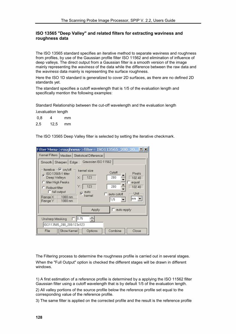
The Scanning Probe Image Processor, SPIP V. 2.2, Users Guide
128
ISO 13565 "Deep Valley" and related filters for extracting waviness and roughness data
The ISO 13565 standard specifies an iterative method to separate waviness and roughness from profiles, by use of the Gaussian profile filter ISO 11562 and elimination of influence of deep valleys. The direct output from a Gaussian filter is a smooth version of the image mainly representing the waviness of the data while the difference between the raw data and the waviness data mainly is representing the surface roughness. Here the ISO 1D standard is generalized to cover 2D surfaces, as there are no defined 2D standards yet. The standard specifies a cutoff wavelength that is 1/5 of the evaluation length and specifically mention the following examples: Standard Relationship between the cut-off wavelength and the evaluation length λ evaluation length 0,8 4 mm 2,5 12,5 mm The ISO 13565 Deep Valley filter is selected by setting the iterative checkmark.
The Filtering process to determine the roughness profile is carried out in several stages. When the "Full Output" option is checked the different stages will be drawn in different windows. 1) A first estimation of a reference profile is determined by a applying the ISO 11562 filter Gaussian filter using a cutoff wavelength that is by default 1/5 of the evaluation length. 2) All valley portions of the source profile below the reference profile set equal to the corresponding value of the reference profile. 3) The same filter is applied on the corrected profile and the result is the reference profile

The Scanning Probe Image Processor, SPIP V. 2.2, Users Guide
129
relative to which the assessment of the profile is performed. 4) The roughness profile is obtained from the difference between the source profile and the reference profile. This is the curve on which roughness parameters should be calculated. This procedure is generalized so that it also works on 2D images even though there are currently no standards for filtering images.
Filter High Peaks An alike procedure can be performed by checking the "filter high peaks" instead of ISO 13565-1 filter deep valleys. This filter removes the peaks instead of the valleys. This is not part of the ISO standard by very useful for filtering instrumentation artifacts often seen in scanning probe instruments.
Robust Filter The Robust Filter is an advanced combination of the Deep Valley and High Peaks filters, as it will minimize the influence from all extreme values in an iterative process: First the image (or profile) is filtered by the plain Gaussian filter The difference between the original and the filter output is generated and the median value of the absolute differences calculated. Extreme points are defined as positions where the absolute errors differs more than two times the median value of the absolute difference. These points are then substituted by the Gaussian filter output. The procedure steps 1-3 are repeated three times. The resulting waviness image is subtracted from the original surface image, which generates the "roughness image" from which robust evaluation of the roughness can be performed.

The Scanning Probe Image Processor, SPIP V. 2.2, Users Guide
130
Non-Linear Filters There are three types of non-linear spatial filters implemented: Median filtering , for noise removal Outlier Objects Filter, for recovery of areas covered by contamination and spike removal Statistical Differencing , for contrast enhancement
Median Filtering The advantage of a median filter is that it is very robust and has the capability to filter only outliers and is thus an excellent choice for the removal of especially shot noise in images. A median filter is performed over a local kernel or mask, the neighbors values are sorted after multiplying them with an importance factor depending on distance or direction. The value in the middle of the sorted buffer, the median value partly determines the acceptable value range for the pixel of interest and it is often used as an replacement value when the pixel value is outside the acceptable range. The following simple example illustrates why median values are more reliable as mean values when searching for outliers and proper replacements: Considering the set "1,3,4,5,8,10, 100,14,16,18,19," the median is 10 and the mean 198/11 = 18. One value deviates extremely from the others and lifts the value of the mean. If this value would be a wrong reading and not included into the calculation of the average, the more correct average would lie closer to the median: (198-100)/10 = 9,8.
Settings It is possible to define kernel shape different from the default rectangular form:

The Scanning Probe Image Processor, SPIP V. 2.2, Users Guide
131
- Rectangular (default) shape - 45 degrees turned rectangle shape - Circular shape ( = octagonal for smaller kernels).
Check at the edges If this option is checked the border-mode is handled as specified in the border-mode settings dialog.
Method The currently implemented median filter is called the RMS Deviation Median Filter , it compares the RMS value , σ(x,y), of the filter mask (excluding the center value) with the center value and the median value m(x,y) within the filter mask. If the pixel value I(x,y) is outside the range:
),(),(),(),(),( yxfyxmyxIyxfyxm σσ +<<− it will be substituted by its median value m(x,y). The acceptance factor f can be set interactively.
Acceptance Factor
The acceptance factor partly determines the acceptance range for individual pixels. The lower the acceptance factor the lower wills the acceptance range be and more pixels will be exchanged. You can work interactively with Acceptance factor to find the value that gives the best result; the filtered result will show up simultaneously when the Auto Apply check box is set. To guide this process the number of modified pixels is indicated in the menu.
Kernel Size The kernel size can be adjusted in both x and y directions. By having for example a 1 × 5 kernel the filter will only be sensitive to corrugations in the y-direction. Kernels for median filters are typically small, lower than or equal 7 pixels in length.
Kernel Preview The kernel Preview shows a limited view of the current shape of the kernel.
Modified Pixels The lower part of the dialog shows the effective modified pixels for the applied filter settings. The last figure shows the amount of percentage of replaced points relative to the complete image contents. In many cases removing between 1-5% of the values would be an effective median filtering, removing outliers without blurring the image. For more noisy images it might be necessary to modify more pixels.

The Scanning Probe Image Processor, SPIP V. 2.2, Users Guide
132
Apply The auto apply button can be checked so that every change in value results in applying the filter to the source image. Otherwise clicking on the Apply button applies the filtering. The auto apply button is more practical with smaller kernels, larger kernels might require more computation time and it might be preferable to turn the current option of.
Example Below is seen an example of an image distorted mostly by short horizontal lines. By defining a 3×7 Median mask we achieve a filter that is extremely selective for this type of artifact. The bottom image shows the difference between the original image and the filtered result. It clearly displays the removed line artifacts and in addition also the "under shoot" artifacts typically occurring when scanning across steep slopes.

The Scanning Probe Image Processor, SPIP V. 2.2, Users Guide
133
The Outlier Objects Filter The Outlier Objects Filter is at strong tool for detecting outliers and filling in the most probable values by interpolation of neighboring pixels, where the aim is to get the truest representation of the image. SPIP will detect a particle when some part of it exceeds a certain level and will then determine its boundaries at the positions where the slope of the particle flattens or changes sign. A user-selected Exchange Method will then fill the pixels inside the particle boundary. Instead of particles it is also possible to detect and remove spikes exceeding a certain slope threshold. The Outlier Objects Filter Menu The Outlier Objects Filter is activated by from the right mouse menu item "Filter Outlier Objects" or from the Processing pull down menu of the SPIP menu bar.
Objects to be removed The upper part of the menu define which object should be removed, Particles, Pores, Spikes or Negative Spikes. And the detection area can be narrowed down to include the Zoom Box Only.
Particles and pores filtering options The Detection Level is set as a percentage of the z-range of the image. Because the Z-range of the image will lower for each filter process it will is possible to filter the image gradually by setting a high detection level and pushing the Apply bottom more times. The detection level will be reflected on the color bar so that you see which part of the images will be handled as objects to be filtered. Likewise you can also define the color bar of the image or the color scale editor. For particles the upper color scale limit will define the threshold value and for pores the lower color scale limit is associated with the threshold value.

The Scanning Probe Image Processor, SPIP V. 2.2, Users Guide
134
Spike filtering options When the "Spike Exceeding Slope" is checked the slope level for detecting a spike can be set. A spike is here defined as a local maximum, or minimum for negative spikes, where the slope dz/dx or dz/dy exceeds the set slope level. Here, we regard maximum values as pixels which two neighboring values in x or the two neighboring values in y are smaller and visa versa for minimum values. There by it is possible to remove structures, which looks like ridges, see example below. Notice, that for scanning probe images the maximum measurable slope is limited by the shape of the tip. If spikes have slopes larger than at the tip apex we have a good indication of a noise artifact, which should be filtered. This spike filter is therefore also very good for preprocessing images before tip characterization, which success depends on how well local maximums can be trusted. The slope of the tip depends may be different seen from different directions and it might also have be mounted so that for example the tip is able of scanning side walls in one direction. I such situations high slopes in one direction may be acceptable but not in the others and therefore necessary to handle the directions individually. To do this you can with the direction check boxes (Up, Down, Left and Right) define which slopes the spike detection algorithm will check against the given slope threshold value.
Exchange Method There six methods for filling new values into the "bad" pixels: Horizontal Interpolation, where new values is inserted by interpolation of the neighboring values in the x-direction. This method is recommended for structures mainly oriented in the x-direction. Vertical Interpolation, where new values is inserted by interpolation of the neighboring values in the y-direction. This method is recommended for structures mainly oriented in the y-direction Min value, where a fixed value equal to the minimum value of the image is entered. Mean Value, where a fixed value equal to the mean value of the image is entered Median Value, where a fixed value equal to the median value of the image is entered Fixed Value, where a value defined by the user is entered
Particle removal example Below is seen an example of an AFM image with a fiber structure suffering from some contamination particles before and after filtration. At the top is the raw image together with at zoom image focusing on two contamination particles and below is seen the same areas after filtration. The Synchronized Multi Zoom function has been used to set the zoom boxes at the exact same locations in the two images. In this case the vertical interpolation method has been applied because the fiber direction is roughly parallel to the y-axis and it is seen that particles has been removed with very little or non-damage to the fibers and we will be able to quantify the fibers much better by the Grain Analysis function.
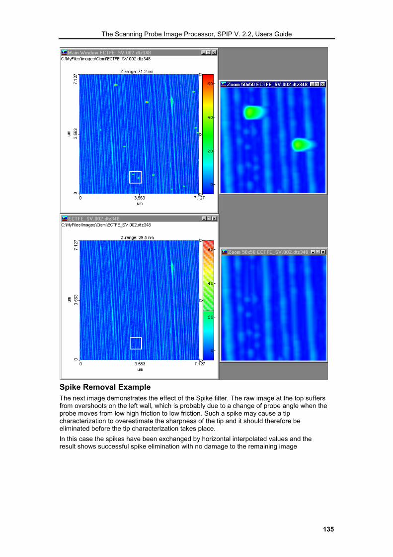
The Scanning Probe Image Processor, SPIP V. 2.2, Users Guide
135
Spike Removal Example The next image demonstrates the effect of the Spike filter. The raw image at the top suffers from overshoots on the left wall, which is probably due to a change of probe angle when the probe moves from low high friction to low friction. Such a spike may cause a tip characterization to overestimate the sharpness of the tip and it should therefore be eliminated before the tip characterization takes place. In this case the spikes have been exchanged by horizontal interpolated values and the result shows successful spike elimination with no damage to the remaining image

The Scanning Probe Image Processor, SPIP V. 2.2, Users Guide
136

The Scanning Probe Image Processor, SPIP V. 2.2, Users Guide
137
Statistical Differencing
Method The statistical differencing menu offers two ways to enhance the contrast: - Local Mean equalization. - Local Standard Deviation equalization. Either one or both methods can be performed on the data set.
Local Mean equalization. This method simply subtracts the mean value of the nearest neighbor pixels within the filter window:
� �−= −=
++⋅
−=2/
2/
2/
2/
),(I1),(I),(ON
Ni
M
Mjjyix
NMyxyx
This is a powerful way to reduce long-range waves and image bow.
Local Standard Deviation equalization The Standard Deviation (SD) equalization scales the height values by a factor given by the SD of the global image, σg divided by the local standard deviation σl found in the filter window.
l
gyxyxσσ
),(I),(O =
This way the local SD and contrast will appear the same all over the image.
Kernel size The filter window, i.e., the number of pixels used for calculation of the local mean and SD values is defined by the X, Y filter kernel Size parameters. To have the desired effect the kernel size should be chosen so that it is larger than the size of the features being studied but smaller that the long range structure, which should be suppressed. When the equal check box is set the X and Y kernel size parameters will be set equal when using the up down buttons.
Auto Apply and Apply The auto apply button can be checked so that every modification of the filter settings will

The Scanning Probe Image Processor, SPIP V. 2.2, Users Guide
138
cause the filter to process immediately so that the effect can be monitored simultaneously. Otherwise clicking on the Apply button will apply the currently defined filter. The auto apply function is a good way to interactively define the filter that gives the best result. However, for larger kernels the response time may be so long that it is more practical to turn off this feature. Below is seen an example of an image filtered by the Statistical Differencing filters: 1 Zoomed portion of a Raw Image with some grains (512×512) 2 Filtered result from a combined Local Mean Equalization and Local SD Equalization filter (Kernels size 45×45). The individual grains are here more visible 3 Difference between the raw image and the filtered image
1 Filtered result from a Local Mean Equalization filter (Kernels size 45×45) 2 Difference between the raw image and the filtered image
1 Filtered result from a Local SD Equalization filter (Kernels size 45×45) 2 Difference between the raw image and the filtered image

The Scanning Probe Image Processor, SPIP V. 2.2, Users Guide
139
Filter Combination Techniques It is possible to define combination of different filters. Two or more single filter kernels can be used to construct a filter combination containing the characteristics of individual filters. This way it is for example possible to combine the edge enhancement filters sensitive to edges in different directions so that the filter combination will be sensitive to all directions. The resulting pixel values are found by combining the output from the different filters in optional ways for example the sum or the maximum of individual output values.
Combination List The list shows the current kernels contained in the filter combination together with their respective sizes. By selecting an item in the list the corresponding kernel can be removed.
Combination Name The Combination Name of the filter is user defined and can be altered. The name of the combined filter will be suggested as file name when saving the filter to the disk.
Remove filter The current selected filter can be removed when this filter is not needed in the filter combination. If wanted all kernels can be removed to create a new combination.
Combination Method The Combination method defines how the results from the individual filter kernels in the list are combined. The following kernel combination modes are currently supported: Supporting Kernel combination modes:
1. Sum the results Summing the results can be good way to combine an edge enhancement or sharpening filter with a smoothing filter.
2. Sum the Squares of the results This method can be used for enhancing all edges and extreme values since negative are treated equally to positive values.
3. Sum the squares of the results and then take the square root This produces sums the square values as above and then applies the square root function. Compared to the Square Sum mode this mode will produce images less dominated by the extreme values and the z-range will be comparable to the z-range of the input image.
4. Takes the maximum of the results This mode can be used with for example edge enhancement, when combining the different

The Scanning Probe Image Processor, SPIP V. 2.2, Users Guide
140
filters with different gradients an edge enhancement can be determined in all 8 or more directions. However, a combination of two or three edge enhancement filters sensitive to for example the East, North and North East directions should be sufficient for this task.
5. Takes the minimum of the results This mode is similar to the above mode but focuses on minimum values.

The Scanning Probe Image Processor, SPIP V. 2.2, Users Guide
141
Unsharp Masking
The lower part of the filter menu contains a "Unsharp Masking" check box and parameter field:
Unsharp masking is a filter technique where the output from a filter is combined with the input image: Depending on the sign of the Unsharp Masking parameter (α) the filter combination will be as follows
),(Filtered),(Iα),(UM yxyxyx +=, for positive values of α
),(Filtered-),(Iα),(UM yxyxyx =, for negative values of α
In the special case where α equals -1.0 and the applied filter is a low pass filter the UM filter becomes a high pass filter: High Pass = Original - Low Pass. This effect can also be obtained automatically by setting the Subtract from Input check box in the Output Option in the Filter Settings. When α > 0, more of the original image is added to the filtered result. ´When the filter type is of high pass type this restores partially the low-frequency components lost during the high-pass filtering operations. The high boost result can also be obtained by increasing the center weight of a high pass or sharpening filter kernel and this way adding more of the original image. For example: a High Pass Filter and a corresponding "high-boost" kernel.
It is easy to work interactively with the kernel center parameter with the dedicated up/down keys:
and this way define the sharpening effect.

The Scanning Probe Image Processor, SPIP V. 2.2, Users Guide
142

The Scanning Probe Image Processor, SPIP V. 2.2, Users Guide
143
ImageMet Explorer
The ImageMet Explorer™, Introduction
The ImageMet Explorer™ is a productivity tool adding a new dimension to image and data handling. It has an integrated database that allows you to browse quickly through your data files and view them as thumbnails. For all recognizable image and curve files thumbnails and other characteristics are automatically entered to the database from where they can be retrieved on the fly while browsing your files. Furthermore, important analytical results from the Scanning Probe Images Processor, SPIP, can automatically be stored in the database so that you never loose important results. You have the flexibility to enter descriptions, assign categories or create hyperlinks to individual files. Although very powerful the usage is so easy that no prior knowledge about data base programming is required.
Image Explorer™ is a combination of three subprograms: ImageMet Browser, ImageMet Finder and ImageMet Reporter which all take advantage of the underlying database:
ImageMet Browser: Organizing and managing files and folders
The browser allows you to browse through your files with an interface and functionality that covers most of what is found in the Microsoft Explorer that is part of your operating system. In addition Image Explorer™ offers thumbnail view for the most common microscope formats and an extra Info Pane where characteristics and results for individual files can be viewed. Furthermore, it is possible to enter descriptions, assign categories and links to related files, web sites, or for example contacts in your contact database file.
ImageMet Finder: Searching for images, files and folders
The ImageMet Finder also covers most of what is found in the search utility of the Microsoft Explorer and additionally it allows you take advantage of the integrated database. It enables searching for images with certain attributes, for example measurement conditions, results within certain ranges, categories, and / or links.
ImageMet Reporter: Reporting data files to HTML
With the ImageMet Reporter you can create HTML reports containing groups of image or profile files. The report can contain graphical presentation of the images or profiles them selves and selected characteristics and results retrieved from the database.
The Image Explorer™ is an optional module of the Scanning Probe Image Processor and its availability depends on your current license.

The Scanning Probe Image Processor, SPIP V. 2.2, Users Guide
144
The ImageMet Browser
The ImageMet Browser is activated from the SPIP program by File�Open or the corresponding tool key and you will see a Browser window similar to the one below:
The ImageMet Browser contains four Panes:
The Folder Pane, upper left, where you can select the directories you want to browse. This window works very similar to the Microsoft Explorer and the same Right-Click functions are provided.
The File List Pane, upper right, where the individual files can be viewed as thumbnails, icons or text lists. Compared to Microsoft Explorer this window has the advantage of being able to visualize all the SPIP recognizable microscope file formats including force curves and profiles. From this window it is possible to select one or more files and open them in the main program.
The Info Pane, lower right, where the characteristics of the selected files can be viewed and edited. Here you can also assign categories and links to related files or e.g. contacts.

The Scanning Probe Image Processor, SPIP V. 2.2, Users Guide
145
The Preview Pane, lower left, where an enlarged view of the selected data files is viewed. The size of the image is determined by the size of the pane and the actual size can be defined by moving the borders between the panes. Images will keep their x,y aspect ratio while curves will be scale to use the full preview area, see the force curve example below:

The Scanning Probe Image Processor, SPIP V. 2.2, Users Guide
146
When you start browsing a directory the first time Image Explorer™ will automatically check if the files are of recognizable formats, in which case the basic information are retrieved and entered into the database together with a thumbnail. Browsing a directory a second time will appear much faster because Image Explorer™ will take advantage of the information stored in the database.
Opening a file:
To open a file, just double click on the file in the File List Pane. If it is a SPIP recognizable file it will be opened in the SPIP program while other files are send to their associated programs. You can force any file to be opened in SPIP by Drag Dropping or clicking on the Send To SPIP tool key. If the file is of non-recognizable format the Read a Special File Format dialog will be invoked and you can instruct SPIP on how to read the file.
It is possible to select more files and open them simultaneously.
Changing the file view mode:
ImageMet Explorer provides four file view modes that can be selected their associated tool keys:
Thumbnail View:
This will limit the view to SPIP recognizable image or curve files for which thumbnails can be created. The size of the thumbnails can be defined in the in the Default View Settings.
Combined Thumbnail and Icon View:
All recognizable files are shown as thumbnails and other files are shown with at default icon.
Small Icons:
All files are shown with their associated icons row wise in the most compact form.
List:
All files are shown with their associated icons column wise.
Details:
All files are shown row wise with columns for Name, Size, Type, Modified time, Description and Categories
Default View Settings
The default view mode at startup can be defined in the Preferences->File List Pane dialog.
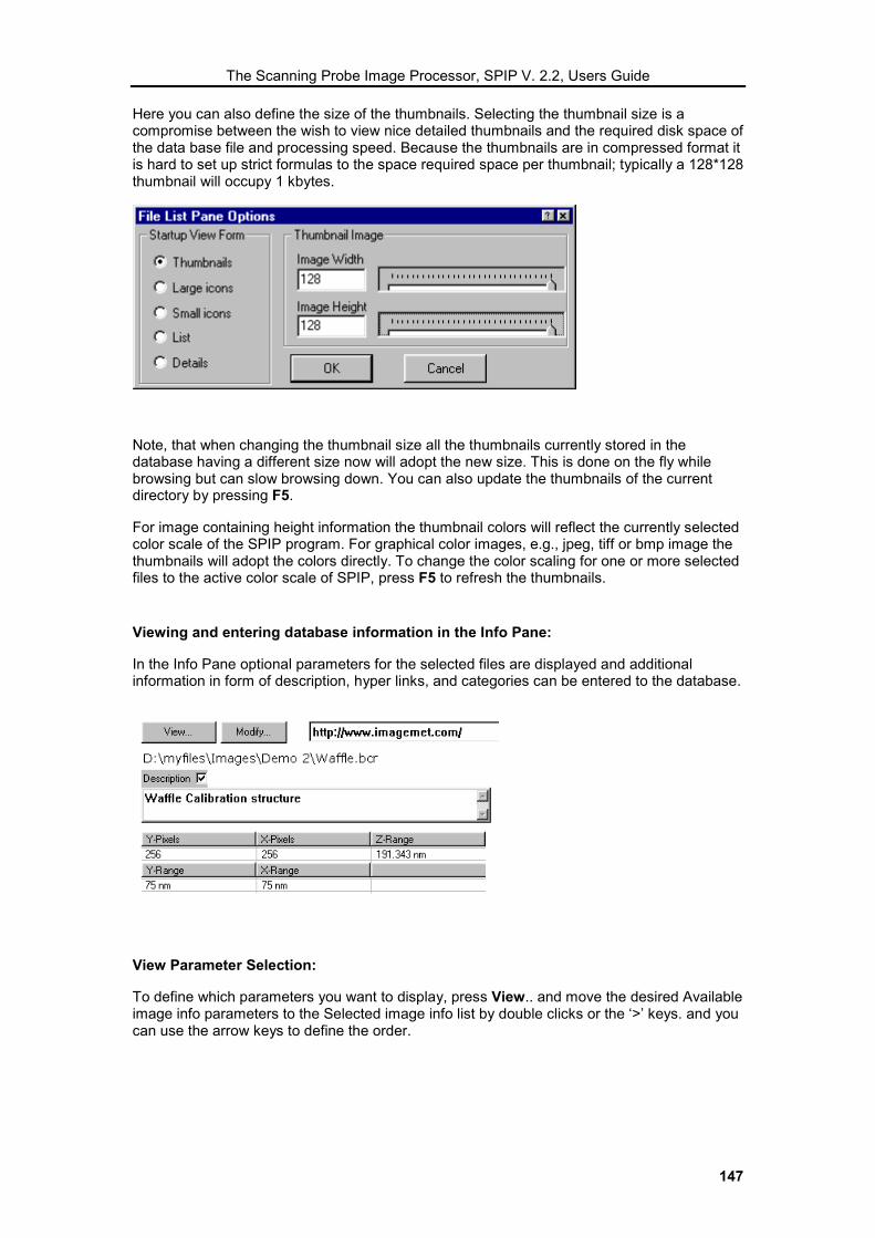
The Scanning Probe Image Processor, SPIP V. 2.2, Users Guide
147
Here you can also define the size of the thumbnails. Selecting the thumbnail size is a compromise between the wish to view nice detailed thumbnails and the required disk space of the data base file and processing speed. Because the thumbnails are in compressed format it is hard to set up strict formulas to the space required space per thumbnail; typically a 128*128 thumbnail will occupy 1 kbytes.
Note, that when changing the thumbnail size all the thumbnails currently stored in the database having a different size now will adopt the new size. This is done on the fly while browsing but can slow browsing down. You can also update the thumbnails of the current directory by pressing F5.
For image containing height information the thumbnail colors will reflect the currently selected color scale of the SPIP program. For graphical color images, e.g., jpeg, tiff or bmp image the thumbnails will adopt the colors directly. To change the color scaling for one or more selected files to the active color scale of SPIP, press F5 to refresh the thumbnails.
Viewing and entering database information in the Info Pane:
In the Info Pane optional parameters for the selected files are displayed and additional information in form of description, hyper links, and categories can be entered to the database.
View Parameter Selection:
To define which parameters you want to display, press View.. and move the desired Available image info parameters to the Selected image info list by double clicks or the ‘>’ keys. and you can use the arrow keys to define the order.

The Scanning Probe Image Processor, SPIP V. 2.2, Users Guide
148
It is possible to create more lists under different names and it can be practical to use names that associates with the parameter types, e.g. Calibration, Roughness
Modifying description, links and categories
To modify or add information in stored in the database press Modify.
Description

The Scanning Probe Image Processor, SPIP V. 2.2, Users Guide
149
Depending on the actual file a description may already have been set at load time. You can edit the description field in free text style.
Categories
For easy and fast search of images for families of images it is convenient to assign logical categories. Press Edit next to the Categories list to define and set new categories:
The categories can be written comma separated in the upper edit field or selected from already defined categories shown below. When entering a non-existing category it will be automatically be added to the Master Category List and made available for other files.
A quick way to find all files belonging to a certain category is by the Category Handler, which is activated from the menu File�Category Handling.
Select the Category you are looking for and press Get all with category
You may also use this menu as a convenient way to assign the same category to all selected files.
Hyper Links:
It can be very convenient to create links to files, data entries or objects associated with a file. Having defined a link you can jump directly to the link with at single mouse click.
To define a new link click on Edit, next to the link list.

The Scanning Probe Image Processor, SPIP V. 2.2, Users Guide
150
You can enter the links directly or browse for a file or Webpage.
Examples of links are:
• c:\myfiles\images\demo\demo-report.doc
• http://www.imagemet.com/
• outlook:Contacts/~Person
Where the latter requires the Microsoft Outlook mail program and is a convenient way to create links to people associated with the file. Similar links may also be created for data fields in other third party file types.
The Scanning Probe Image Processor, SPIP V. 2.2, Users Guide
151
Common Tasks Copy and Move a file(s) or folder(s)
Click the drive or folder you want to work with.
Click the file or folder you want to copy or move.
Cut: This button corresponds to Edit→Cut and cuts a selected object to the clipboard.
Copy: This button corresponds to Edit→Copy and copies a selected object to the clipboard.
Paste: This button corresponds to Edit→Paste and places the content of the clipboard to the selected folder
To select consecutive files or folders to copy or move, click the first item, press and hold down SHIFT, and then click the last item.
To select files or folders that are not consecutive, press and hold down CTRL, and then click each item.
To select all files press CTRL+A.
It is advised to copy the different files and folders by use of ImageMet Explorer if you do want the same changes performed on the database; otherwise some of the information might not get linked correctly.
Browsing shared folders on another computer over the network
Browsing files over the network is like browsing your locale computer, but depending on how the network is configured it will appear slower.
To locate files on another computer click on My Network Places or Network Neighborhood.
Locate the computer in which the shared folder is located.
Choose the shared folder you want to browse.
You can assign a drive letter for shared folders that you connect to often.
To map a drive letter to a network computer or folder follow the following description:
Open Windows Explorer.
On the Tools menu, click Map Network Drive.
In Drive, select the drive letter to map to the shared resource.
In Folder, type the server and share name of the resource, in the form of \\servername\sharename. Or click Browse to locate the resource.

The Scanning Probe Image Processor, SPIP V. 2.2, Users Guide
152
Change file or folder properties
Right-click the file whose properties you want to change.
On the File menu, click Properties.
To change properties for archiving, indexing, compression, or encryption on NTFS drives, right-click the file, click Properties, click Advanced, and then select the options you want to change.
Tool key supported functions
Most common functions can be accessed directly from the toolbar and/or by short cut keys:
Selects the parent folder of the current folder in the directory tree
Ctrl +X: Cuts one or more selected objects to the clipboard.
Ctrl + C: Copies one or more selected objects to the clipboard
Ctrl + V Places the content of the clipboard to the seleced folder.
F8 Changes the view mode to thumbnail mode. Only data files for which a thumbnail can be created are shown, the size of these can be set in the preferences dialog.
F9 Shows thumbnails for recognizable files and icons for other files, the size is dependent of the settings in the preferences dialog.
F10 Shows a file list with small icons and names
F11 Shows a file list with small icons and names
, F12 Shows details, with name, size, type, modified time, description from the data base and categories
File→Find Activates the ImageMet Finder, from which files with certain characteristics can be found. The results will be shown in the File View Window and the Info View and Image Window will reflect selected files.
File�Report Enables the ImageMet Reporter for the currently selected files. If nothing is chosen than it is assumed that the complete content of the listview or all the viewable thumbnails will be used.
Use this button to open this file or several in the SPIP program.
Start the help program.

The Scanning Probe Image Processor, SPIP V. 2.2, Users Guide
153
Dynamic Capture of Results
One of the strong features of the ImageMet Explorer™ is the possibility for adding results to the database automatically when they are produced. To define which type of results should be entered to the database activate the Options dialog from the menu bar of the SPIP main program:
Currently five different types of results can be entered to the database:
• Lateral Calibration
• Height Calibration results
• Grain / Pore statistical results
• Linearity errors and correction parameters
• Roughness Parameters
• Tip Characterization results
When performing tests on e.g. the influence of preprocessing techniques it can be convenient to turn off all updates of the database to assure that previous results are not overwritten. Un-checking Use ImageMet Explorer can do this. Note, by turning off Use ImageMet Explorer ImageMet Explorer will not be activated on File����Open, instead files are opened in the traditional way.
If you for some reason should want to remove the results stored for at given file you can in the File List Pane select one or more files and then right click on Reset Results in Database, which will remove all results.

The Scanning Probe Image Processor, SPIP V. 2.2, Users Guide
154
The ImageMet Finder
To activate ImageMet Finder click the corresponding tool key or select the menu item File����Find. You will see that the ImageMet Finder menu is very alike the find menu of Microsoft Explorer, but with additional search capabilities for parameters that can be extracted from the files a stored in the database.
Note, you can use the ImageMet Finder to build up the ImageMet database in one step; by entering the wildcard symbol ‘*’ and setting the Database check box Submit found images to database all files in the selected directory and its subdirectories will enter the database with thumbnails and other characteristics. Depending on the number of data files this make take a while but afterwards you will be able to browse all the directories much faster and searching for files will also be functioning faster.
The search result will be displayed in the File List Pane of the ImageMet Browser where you can investigate the files for further details, load them into the main program or create a report using the ImageMet Reporter. Name Tab
Use the fields in the Name Tab do define names and locations for the files you want to find. It is possible to use wildcards and an empty name field will be regarded at * enabling us to find all files in a given directory tree. Date Tab
Select the Date tab to specify file modification time intervals for the search criteria. Database files
Select the Database tab to enter search criteria related to recognizable image or curve files.
Found files not already included in the database can be submitted to the database automatically when the Submit to Database check box is set. The search criteria can also be

The Scanning Probe Image Processor, SPIP V. 2.2, Users Guide
155
limited by checking the checkbox Search only files submitted to database. When this selection is chosen more specific search criteria can be used.
Click Find Now to start finding the files satisfying the entered search criteria. During the search process you will have the option to stop the searching by pressing the Stop push button

The Scanning Probe Image Processor, SPIP V. 2.2, Users Guide
156
The ImageMet Reporter
The ImageMet Reporter is designed for creation reports containing catalogs of selected data files, including the images or curves themselves together with its characteristics and calculated results.
To create a report first select the images in the File List Pane, which you want to include in the report, then activate the ImageMet Reporter by it associated tool key and define the output settings.
If no files have been selected the reporter will include all files in the current directory. Note also that it is possible to create reports including more folders by selecting files from the output of the ImageMet Finder
Format
The currently available format is the HTML format, which makes it easy to include your data on web sites.
General Reporting Options
It is optional to include image of optional size or just to show the filename.

The Scanning Probe Image Processor, SPIP V. 2.2, Users Guide
157
Reporting Style
The report can be written in two styles:
The Plain style where the files with the selected characteristics are shown row wise below each other.
The Tabular style will create a report with one column per file, with the image and file name shown on top and below the selected data fields.
Data Fields
From the available data base fields you can choose which you want to have included in the database. The available fields are the same as seen in the File Info Pane and at the lower left you can conveniently select predefined groups of fields or define new groups
Report generation and viewing
The report generation will start when clicking the OK button and when finished your default web browser will open and show the results. If you want have the report to appear differently just change the options and click OK again. Depending on your browser it might be necessary to perform a refresh to update the file content the 2nd time.
Below is shown a typical report defined with 3 columns and image of the size of 100 x 100 pixels.

The Scanning Probe Image Processor, SPIP V. 2.2, Users Guide
158

The Scanning Probe Image Processor, SPIP V. 2.2, Users Guide
159
SPIP Plug In Interface for Programmers The intension of the SPIP Plug In interface is to provide and easy way for users to exchange data with the SPIP program. There are mainly three types of operations you can perform with the interface.
1) Retrieve Images or curves from SPIP windows and apply your own specialized analysis software.
2) Manipulate data by your own algorithms and view the result in the SPIP windows. 3) Create your own data and use SPIP’s analytical and visualization tools. The data can
come from your own control and data acquisition software integrated with SPIP, your own file reader or artificial created data.
This way you get all the advantages of all the SPIP processing features including file handling and visualization while you can concentrate on your own specialized data processing and data creation. You can get easy access to your functions by defining associated buttons that will appear in the SPIP Menu. Your plug-ins can include data processing functions as well as dialogs. The following is a short Getting Started Introduction, the SPIP Plug In Functions section of the reference guide contains more detailed information about the available interface functions. Compilers If you have the Microsoft Visual C++ 6.0 or the Microsoft Visual Basic 6.0 available the easiest way to create a SPIP Plug In Interface is through the SPIP Plug In Wizards, which will create a complete project including example code ready to build and run. For the Borland C++Builder 5 an example project is included. For other compilers you may from the Borland example and the projects created by the wizards see how a project is structured and adapt it to the compiler. The interface is based on COM technology and every programming environment than can create plain DLLs, COM DLLs or ActiveX DLLs can be applied for creation of SPIP Plug Ins. Below is described how to use the SPIP Plug In Wizard for MS Visual studio and how to build and run the Borland C++Builder example. User Prog Menu and Programming Tools: In addition to the user defined Plug Ins the User Prog menu contains a number of convenient functions.
Repeat Last Function will repeat the most recent plug in function that has been processed and its shortcut is Ctrl+Shift+Y.

The Scanning Probe Image Processor, SPIP V. 2.2, Users Guide
160
The Define User Source Window function is useful when using user-defined dialogs. When a user dialog is created it will be connected to the active data window, - the User Source Window. Whenever the dialog retrieves data it will get it from the User Source Window. However, another data window can be defined as the User Source Window by clicking Define User Source Window or just Ctrl+W. Programming Tools The User Prog menu comes with a predefined submenu called Programming Tools, where you find useful utilities that can be applied when creating and trouble shooting your own plug ins. Show Available User Functions. To get information on the available DLLs and plug in functions click on Show Available User Functions. The DLL Linker Dialog will then show a list of available DLL files. It will be indicated if the DLLs include the SPIPExport function necessary for creating the User Menu. Likewise, the presence of the CloseDLG function is indicated; For C++ projects SPIP needs to call this function when closing plug in dialogs. The Version number is associated the data exchange functions and used for checking the comparability with the current SPIP version. For each DLL you can get information about the available plug in functions, their source code name, number in the User Prog menu, Menu item name and the name of its menu group, and you have to possibility to process the functions from the dialog by clicking Execute.
Close All Dialogs will close all user defined dialogs. Close All DLLs will close all user defined dialogs and free the connections to the DLLs. This enables you to modify and test a plug in without having to restart SPIP. The Start MS Visual C++, Start MS Visual Basic, and Start Borland C++Builder menu items are provided for your convenience and will be active when the associated compilers are found present on the computer.

The Scanning Probe Image Processor, SPIP V. 2.2, Users Guide
161
SPIP Plug In Wizard for Microsoft Visual C++ 6.0
Installation The following procedure requires that Microsoft Visual Studio C++ 6.0 be installed on your computer. If so, the SPIP Plug In Wizard will automatically be installed the first time you click on the User Prog in the SPIP menu bar. Using the Wizard
1) Activate the MS C++ 6.0 development studio from your task bar or conveniently from SPIP→→→→User Prog→→→→ Programming Tools→→→→Start MS Visual C++.
2) In Visual C++ select File→→→→New and in the Projects Tab select SPIP Plug In Interface Wizard and enter a proper Project Name, for example MySPIPPlugIN and the file location for the project.
Click OK
3) In the step 2 dialog click the Create a Dialog check box if you want a dialog to be included.

The Scanning Probe Image Processor, SPIP V. 2.2, Users Guide
162
4) You can now click Finish or click Next to set some other standard project options. 5) After clicking Finish the project is automatically generated. 6) The Project is now ready go be build: click Build→→→→Build MySPIPPlugIn.dll and the
resulting dll will put into the SPIP\UserDLL folder where it is automatically found by SPIP next time SPIP is started and the menu items defined in the project are automatically inserted in the SPIP→User Prog menu. The predefined example functions are called Tilt X Up, Tilt X Down, Create Periodic Image and Invert Data Dialog. You can modify these functions and use them as inspiration for new plug in functions.
7) Restart SPIP and try to click on the Plug In example Menu Items found in the SPIP→→→→User Prog menu.
Modifying the Code. The files generated by the wizard can be viewed in the FileView of the project. You need just to concentrate on the MySpipPlugIn.cpp and the MySpipPlugInDlg.cpp files, - the latter is not generated if you decided not to include a dialog in the project.

The Scanning Probe Image Processor, SPIP V. 2.2, Users Guide
163
The only SPIP class you need to know is the CSpipExchange class, which contains methods for retrieving and sending data to and from SPIP Windows. Once a CSpipExchange object is defined a connection between the object and the SPIP program is created. Below is seen the simple TilXUp() example function, which retrieves the data from the active SPIP client window and add the x pixel index to the pixel values. Finally the modified image is displayed in the SPIP source window.
extern "C" _declspec(dllexport) int TiltXUp(){
CSpipExchange b;
if (!b.Get_ImageData()){::AfxMessageBox("No data in window",MB_OK,NULL); return 0;}
int i = 0;for (int y=0;y<b.SizeY;y++)
for (int x=0;x<b.SizeX;x++, i++){b.Data[i] += x;
}// Show the tilted image in the source windowIM_PWIN pShow=NULL;b.Show_ImageData(&pShow,"TiltX",IMF_SOURCE);return true;
}
You can modify this code to suit your needs or copy it to a new functions with a different names. To define the Plug In functions that should appear as Menu Items in the SPIP program one call to AddToSPIP for each Plug In function should be included in the SPIPExport() function:
void SpipExport(){AddToSPIP("TiltXUp" ,"Tilt X Up", "Group MySpipPlugh",0 );AddToSPIP("TiltXDown" ,"Tilt X Down","Group MySpipPlugh",0 );AddToSPIP("PeriodicImage","Create Periodic Image","Group MySpipPlugIn",0 );AddToSPIP("InvertDataDialog","Invert Data Dialog","Group MySpipPlugIn",0 );
}
The first parameter in the AddToSPIP function should be identical to the name of the function (except for Borland compilers where you need to include an underscore in front of the name,

The Scanning Probe Image Processor, SPIP V. 2.2, Users Guide
164
e.g., _TiltXUp ). The second parameter is the friendly name that will appear as the menu item text. The third parameter is the Group Name, which enables you to group the Plug In functions to different submenus; when setting this parameter to NULL the menu item will appear at the outer level. The last parameter is reserved for future use of icons. Modification of the dialog To design the dialog click the ResourceView tab in the Workspace and double click the first dialog. After for example a button you can go to its event handler by double clicking on it. Here you can enter the desired function of associated with the button. Refer to the MS Visual C++ documentation for more details on how to create new buttons and setting up event handlers. Debugging the Code. Debugging of the Plug In code can be performed from the Visual C++ environment, just select Build→→→→Start Debug→→→→Go and enter the spip.exe program as the executable file. To rebuild the project and restart a debug session you will need to unload your DLL by pressing User Prog→→→→Programming Tools→→→→Close All DLLs alternatively you will need to restart SPIP. After creating complete new menu items it is necessary to restart SPIP. For further information about the available functions refer to SPIP Plug In Functions For C++ in the reference guide.

The Scanning Probe Image Processor, SPIP V. 2.2, Users Guide
165
Borland C++ Builder Example The SPIP package comes with an example project for Borland C++Builder version 5. The following describes a step by step procedure for installing, building and running the project:
4. Create at new folder for the Borland Plug In project. 5. Find the BorlandPlugIn.zip in the SPIP\Programming Resources folder and unzip its files
to your newly created project folder. 6. Open the project BorlandPlugIn.bpr now found in your project folder. 7. Click Project����Options and select the Directories/Conditionals tab and set the Final
output to the SPIP\UserDLL folder.
8. Define also where you want the Intermediate output files and remember to create this
folder if it does not already exist. 9. To build the project select Project����Build BorlandPlugIn or the associated shortcut key. 10. You should now have a BorlandPlugIn.dll file installed in the SPIP\UserDLL directory
containing three plug in functions, which SPIP automatically will recognize next time you start SPIP. To start and debug your dll from inside Borland Builder define first the Host Application; select Run����Run Parameters and enter the path for the spip.exe host program.

The Scanning Probe Image Processor, SPIP V. 2.2, Users Guide
166
Select Run����Run SPIP should now start and you will find your three menu items associated with your plug in functions in User Prog����BorlandPlugIn menu group.
To modify the code you should concentrate on the BorlandPlugIn.cpp file, see the description in the Modifying the Code Microsoft section above.
For further information about the available functions refer to SPIP Plug In Functions For C++ in the reference guide.
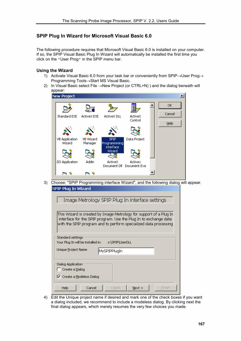
The Scanning Probe Image Processor, SPIP V. 2.2, Users Guide
167
SPIP Plug In Wizard for Microsoft Visual Basic 6.0
The following procedure requires that Microsoft Visual Basic 6.0 is installed on your computer. If so, the SPIP Visual Basic Plug In Wizard will automatically be installed the first time you click on the "User Prog" in the SPIP menu bar.
Using the Wizard
1) Activate Visual Basic 6.0 from your task bar or conveniently from SPIP→User Prog→ Programming Tools→Start MS Visual Basic.
2) In Visual Basic select File →New Project (or CTRL+N) ) and the dialog beneath will appear:
3) Choose: "SPIP Programming interface Wizard", and the following dialog will appear.
4) Edit the Unique project name if desired and mark one of the check boxes if you want
a dialog included, we recommend to include a modeless dialog. By clicking next the final dialog appears, which merely resumes the very few choices you made.
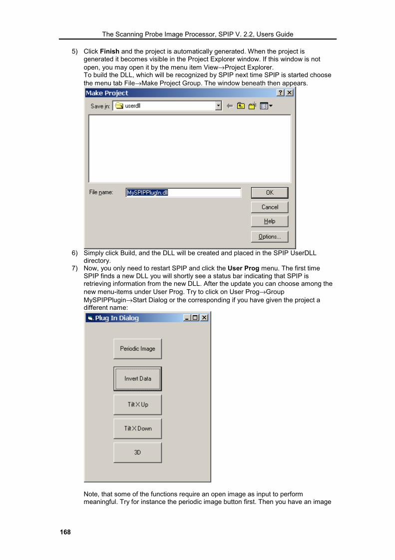
The Scanning Probe Image Processor, SPIP V. 2.2, Users Guide
168
5) Click Finish and the project is automatically generated. When the project is generated it becomes visible in the Project Explorer window. If this window is not open, you may open it by the menu item View→Project Explorer. To build the DLL, which will be recognized by SPIP next time SPIP is started choose the menu tab File→Make Project Group. The window beneath then appears.
6) Simply click Build, and the DLL will be created and placed in the SPIP UserDLL
directory. 7) Now, you only need to restart SPIP and click the User Prog menu. The first time
SPIP finds a new DLL you will shortly see a status bar indicating that SPIP is retrieving information from the new DLL. After the update you can choose among the new menu-items under User Prog. Try to click on User Prog→Group MySPIPPlugin→Start Dialog or the corresponding if you have given the project a different name:
Note, that some of the functions require an open image as input to perform meaningful. Try for instance the periodic image button first. Then you have an image

The Scanning Probe Image Processor, SPIP V. 2.2, Users Guide
169
to work on.
Modifying the Code.
The files generated by the wizard can be viewed in the Project Group window, if not active press View�Project Explorer. You need only to concentrate on the CProcessing, CExport and FDialog files, - and the latter is only generated if you decided to include a dialog in the project. You may also view the CAverage class to learn how averaging of multiple images or curves can be performed.
Modifying the Dialog To enter new buttons in the dialog double click on FDialog, and use the Form editor to design the dialog:

The Scanning Probe Image Processor, SPIP V. 2.2, Users Guide
170
The event handlers of the individual buttons can be viewed and modified after double clicking the buttons:
You will see that the code in Fdialog module is very short because it makes use of the functions defined in CProcessing, which includes all the data processing, see for example the code for inverting an image:

The Scanning Probe Image Processor, SPIP V. 2.2, Users Guide
171
This code retrieves an image (or curve) from SPIP, changes the sign of all points, modifies the file name and shows the result in the source window. As indicated in the passive code the image could also have been shown in independent SPIP windows for example in the 3D window. Creating new functions When creating you own functions it can be an advantage to use the above code as a template, simply use copy & paste modify the code to suit the task and change the function name. Adding new menu Items To give SPIP knowledge and access to your functions they need to be published in the SPIPExport module by a function called SpipExport (do not change this name):
There is one AddToSpip call for each function that will appear in the User Prog menu. The second parameter is the exact name of the function, the third parameter defines the name of the function as it will appear in the menu and the last parameter specifies the name of the menu group in which this item will be put. Just by using other names other menu groups will be created.
For further information about the available functions refer to SPIP Plug In Functions For Visual Basic in the reference guide

The Scanning Probe Image Processor, SPIP V. 2.2, Users Guide
172

The Scanning Probe Image Processor, SPIP V. 2.2, Reference Guide
173
Reference Guide


The Scanning Probe Image Processor, SPIP V. 2.2, Reference Guide
175
Fourier Analysis The Fourier transform is a powerful tool for image analysis. This is true in particular for analysis of repeated patterns such as pitch standards and molecular or atomic structures. Fourier images reflect repeated patterns as narrow peaks, the co-ordinates of which describe their periodicity and direction. Such peaks are easy to detect by image processing without any pre-knowledge of the features form or periodicity. Furthermore, the repeat distances can be measured very accurately by determining the Fourier peak co-ordinates at sub-pixel level. The discrete Fourier transform is calculated by the formula:
� �−
=
−
=
+−=1
0
1
0
)//(2),(1),(x y
yxN
x
N
y
NvyNuxi
yx
eyxzNN
vuF π ,
(1)
where Nx, Ny are the number of pixels in the x,y directions and u,v the discrete Fourier indexes:u=0,1,2,..Nx-1 and v = 0,1,2..Ny-1. The Fourier transform can also be regarded as a sum of sinusoidal functions, each described by a frequency, amplitude and a phase. The inverse transform, which, for example, may be applied after filtration where, for example, unwanted Fourier components are set to zero, has a similar form:
� �−
=
−
=
+=1
0
1
0
)//(2),(),(x y
yxN
u
N
v
NvyNuxievuFyxf π
,
(2)
The number of computational operations can be reduced dramatically by Fast Fourier Transform (FFT) algorithms that breaks the calculation down to a sequence of smaller Fourier transforms. The highest efficiency is obtained when the side lengths Nx and Ny are powers of 2. Thus, typical images are 256 × 256 or 512 × 512 pixels. The chosen size is a compromise between a high pixel density and the costs in form of extra acquisition time, storage demands and calculation time. The Fourier transform can be visualized by its amplitude spectrum, which are the absolute values of the complex Fourier components:
),(),(),( 22 vuIvuRvuF += ,
(3)
where R and I denote the real and imaginary parts respectively. The phase information is rarely used but preserved in case inverse transformations have to be applied after exclusion of some Fourier components. To enhance the contrast of weaker components a square root function or logarithmic function may be applied to the amplitude values. Likewise, more dominant components may appear with even higher contrast when the amplitude values are squared. Contrast changes by color manipulation may also be a valuable technique to reveal weak Fourier components.

The Scanning Probe Image Processor, SPIP V. 2.2, Reference Guide
176
Detecting Line Profiles Periodic surface features will exhibit peaks corresponding to the periodicity in the Fourier amplitude image. For a spatial image of k line profiles parallel to the y-axis we will in the Fourier image have a peak at (u,v) = (k,0). For profiles not aligned parallel to one of the axes, but where k periods can be counted along the x-axis and l periods along the y-axis a Fourier peak can be found for (u,v) = (k,l). The corresponding wavelength λ is easily calculated:
λ =���
��� +
�
��
�
��
wl
wk
x y2 2
,
(4)
where wx and wy are the physical x, y ranges of the image. When the number of periods differs from an exact integer the real Fourier peak is not part of the discrete components of equation (1) and therefore is not calculated. However, due to the picket fence effect the neighboring Fourier elements will exhibit higher values from which the real frequency can be estimated by inverse interpolation or by an iterative sub-pixel Fourier algorithm. The sub-pixel Fourier algorithm makes it possible to calculate Fourier components also for non-integer u,v co-ordinates just by entering those values directly into equation (1) and thereby get sub-pixel resolution. To obtain a good computation efficiency the u,v co-ordinates are only calculated within a pixel distance from the peaks found at pixel level. Within these areas, a steepest ascent algorithm can locate the peaks. For regular patterns, which are not of sinusoidal form the structure can not be described by a single Fourier component only. The Fourier transform will then consist of a fundamental peak at (u0,v0) associated with the main periodicity and by higher harmonics, i.e. components for which the (u,v) co-ordinates are n times higher than the fundamental Fourier component:
(un,vn) = n (u0,v0). (5)
This can be an advantage because we can obtain from each harmonic an estimate of the fundamental component by dividing co-ordinates by the harmonic number:
( , ) ( , ) /' 'u v u v nn n0 0 = . (6)
Thus, it is possible to obtain a statistical mean value for the fundamental Fourier component. The advantage of this use of the higher harmonics is also that the uncertainty of the (u,v) co-ordinates are divided by the harmonic number. However, higher Fourier harmonics are usually weaker and are therefore harder to estimate accurately. It is therefore impossible to predict from which harmonic components we get the most accurate estimate of the fundamental component, as it will depend on the measurement object as well as the measurement conditions. The accuracy may also be influenced by false detection, for example electrical noise might mistakenly be regarded as a harmonic component associated with the repeated surface structure. To make statistical estimation of the fundamental periodicity based on higher harmonics more robust it is an advantage to use the median value instead of the mean value.

The Scanning Probe Image Processor, SPIP V. 2.2, Reference Guide
177
Detecting Unit Cells The oblique unit cell
The arrangement of repeated units of periodic patterns can be described by a Bravais lattice. The units may be individual atoms, molecules or, for example, artificially created calibration structures. The two dimensional Bravais lattice summarizes the geometry of the periodic structure, and consists of all points with position vectors S of the form:
S=k a + l b , (7)
where a and b are any two dimensional vectors of different and k, and l range through all integer values. An area on the surface that, when translated through all the vectors in a Bravais lattice just fills all of the surface without either overlapping itself or leaving voids, is called a primitive unit cell of the lattice, and the a and b vectors are then called primitive vectors. There is no unique way of choosing a primitive unit cell for a Bravais lattice and they can have different forms: square, hexagonal (rhombus), rectangular or oblique. The oblique unit cell is general and we will use this in the following. Note also that even though the calibration structure is quadratic the distortions are most likely to create images with oblique unit cells. By Fourier transform of a Bravais lattice a reciprocal lattice K is created with Fourier peaks that can be described by the reciprocal unit cell vectors A and B:
K=k A + l B , (8)
where k, and l range through all integer values. The important property of the Fourier transform is that the reciprocal unit cell vectors can be found directly from the positions of the peaks. Having found the A and B reciprocal unit cell vectors the spatial unit cell vectors a and b can be found as
BA
AbBA
Ba −
−
−
−== ;_
(9)

The Scanning Probe Image Processor, SPIP V. 2.2, Reference Guide
178
Lateral Calibration by Quadratic Unit Cells To describe the correspondence between the observed surface lattice and the real physical lattice, we use the transformation matrix. Here we will ignore non-linearity and the influence from the z-axis. We arrange the co-ordinate system of the uncorrected and the correct co-ordinate systems so that their x-axes are parallel.
xy
C CC
xy
x xy
y
�
��
�
�� =
�
��
�
��
′′
�
��
�
��0
, (10)
Where Cx, Cy and Cxy are the unknown correction parameters to be estimated. If the scanned x- and y-axes are perpendicular, then Cxy equals zero and Cx,Cy are the scale factors for the x- and the y-directions respectively, i.e., x C xx= ′ and
y C yy= ′.
Cxy describes the coupling between the x and y axes, i.e. how much the scanner moves in the x-direction when stepping in the y-direction. The angle γ between the scanned x-axis and the scanned y-axis is given by
( )γ = −cot 1 C Cxy y and the angular distortion γe = 90°-γ. When using a calibration standard with square unit cells described by a repeat distance, L, then based on the observed unit cell vectors
a' b'=�
��
�
�� =
�
��
�
��
aa
bb
x
y
x
y,
and the reference value l we can find an analytical solution for the three unknown correction parameters:
CL a ba b a b
CL
a bC
b b a a L
a b a b a bx
y y
x y y xy
y yxy
y x x y
x y y x y y
=+
−=
+=
+
− +
2 2
2 2 2 2, ,
( )
( )
(11)
Off-line correction of images can be performed by re-sampling at equidistant (x’,y’) positions.
x x yC x C y
C Cy x y y Cy xy
x yy' ( , ) , ' ( , ) /=
−=
.
(12)

The Scanning Probe Image Processor, SPIP V. 2.2, Reference Guide
179
Lateral Calibration by Hexagonal Unit Cells Calibration by hexagonal lattices can be done very similarly to the calibration by square lattices. However, the equations to calculate the linear correction parameters are different:
CL a b a b
a b a b
CL
a b a b
Ca a b b a b a b L
a b a b a b a b
xy y y y
x y y x
yy y y y
xyx y x y y x x y
x y y x y y y y
=+ −
−
=+ −
=+ − −
− + −
2 2
2 2
2 2
32
2 2
2
,
,
( )
( )
(13)
It is not possible to calibrate the Cx, Cy and Cxy parameters by a single image of line structures. Only by careful alignment of the structure along the X or Y-axis, it is possible to deduce the Cx or the Cy parameters. However, by acquiring three images of a line structure rotated at three different angles is possible to setup an equation system from which the three correction parameters can be deduced: In a Fourier transformation of an image with a line pattern, a wave vector K with a high intensity will be observed. It can be shown that the wave vector K=(u, v)T†of the corrected image is related to the wave vector K´=(u´, v´)T of the uncorrected image through the transformation K=(C-1)TK´, or
uv C C
CC C
uvx y
y
xy x
�
���
�� = −
�
��
�
��
′′
�
��
�
��
1 0
(14)
Furthermore the reciprocal length |K|-1 of the wave vector K=(u, v)T is equal to the known periodicity 1/λ of the. That is:
K 2 2 2 21= + =( ) ( ) /u w v wx y λ (15)
By combining the equations a restraint between Cx, Cy and Cxy and the known period r is obtained. Thus, for three images with different orientation of the lines, an analytical solution for Cx , Cy and Cxy is found. For more than three images the restraint form an over-determined system of equations in the unknowns Cx, Cy, and Cxy. A least squares sum solution of this equation system can then be found.

The Scanning Probe Image Processor, SPIP V. 2.2, Reference Guide
180
Lateral Linearity Analysis
This advanced process can be started directly by pushing the associated key: From the detected lattice structure, we can predict the position of repeated features by knowing the position of a single feature belonging to the lattice. We therefore select a single feature (template) representative of the lattice and by cross correlation we find the position of the other matching features. If the zoom image is active it will define the template which has to be recognized otherwise SPIP automatically finds a suitable template based on a detected unit cell. The positions are identical to the peaks in the cross correlation function, which we estimate at sub-pixel level by parabolic fits. These positions are compared with the predictions based on the unit cell vectors and we calculate a prediction error vector ek,l:
)'''(' 0,0,, bappe lklklk ++−=, (16)
where p' ,0 0 is the vector pointing to the highest peak in the cross correlation function and
p' ,k l the pointing vectors to the peaks in the cross correlation function that comes closest to ( ' ' '),p a b0 0 + +k l
. The integers k,l are found so that ek,l is minimized. The prediction error, ek,l, typically reflects non-equidistant sampling during scanning. However, imperfections of the sample or environmental conditions might also be reflected in the result. Keeping k,l fixed it is possible to adjust the unit cell vectors a’,b’ by minimizing the mean position error:
EMu k l
k l= �
1| |,
,e
,
(17)
where M is the number of peak vectors in the cross correlation image. We can thereby find an alternative calculation of the unit cell that can be compared with the one calculated from the Fourier domain. Eu also serves as a measure of the non-linearity; the smaller it is the better. We can visualize the prediction errors for the x, y co-ordinates of ek,l independently as
function of their x, y co-ordinates peak position co-ordinates of p' ,k l , see d,e, and it is
possible to estimate polynomial fits to the data and obtain correction functions. From the
curve describing the x-co-ordinate error, e px x( ' ) we calculate the physical scanning co-ordinate:
p p p e (px x x x x( ' ) ' ' )= − (18)
To resample the image at equidistantly separated points a model that describes the observed
co-ordinates as function of the physical co-ordinates can be applied. The observed p x' co-
ordinates can be modeled by a function of the physical positions px by a least mean square polynomial fit

The Scanning Probe Image Processor, SPIP V. 2.2, Reference Guide
181
p x a x_
xn
N
nn' ( ) =
=�
0 ,
(19)
where N is the polynomial degree and the an coefficients found by minimizing the error function Ex:
E (p' a p )x x n xn
n
N
= −� �=0
2
.
(20)
Here the summation goes over all detected peaks in the cross correlation function.

The Scanning Probe Image Processor, SPIP V. 2.2, Reference Guide
182
Calibration by Line Structures It is not possible to calibrate the Cx, Cy and Cxy parameters by a single image of line structures. Only by careful alignment of the structure along the X or Y-axis, it is possible to deduce the Cx or the Cy parameters. However, by acquiring three images of a line structure rotated at three different angles is possible to setup an equation system from which the three correction parameters can be deduced: In a Fourier transformation of an image with a line pattern, a wave vector K with a high intensity will be observed. It can be shown that the wave vector K=(u, v)T†of the corrected image is related to the wave vector K´=(u´, v´)T of the uncorrected image through the transformation K=(C-1)TK´, or
uv C C
CC C
uvx y
y
xy x
�
���
�� = −
�
��
�
��
′′
�
��
�
��
1 0
(14)
Furthermore the reciprocal length |K|-1 of the wave vector K=(u, v)T is equal to the known periodicity 1/λ of the. That is:
K 2 2 2 21= + =( ) ( ) /u w v wx y λ (15)
By combining the equations a restraint between Cx, Cy and Cxy and the known period r is obtained. Thus, for three images with different orientation of the lines, an analytical solution for Cx , Cy and Cxy is found. For more than three images the restraint form an over-determined system of equations in the unknowns Cx, Cy, and Cxy. A least squares sum solution of this equation system can then be found.

The Scanning Probe Image Processor, SPIP V. 2.2, Reference Guide
183
Output File Formats SPIP currently supports three file output formats in which images and curve data can be saved:
*.bcr The BCR-STM file format, binary; preserves physical dimension data; applies to 2D image and curves including histogram.
*.asc ASCII file format for import in other programs; preserves physical dimension; applies to 2D image and curves including histogram
*.bmp Bitmap, for import in most DT programs; applies to all graphical windows. To save your images in other graphics file formats you can always Copy and Paste the windows content into third party programs.

The Scanning Probe Image Processor, SPIP V. 2.2, Reference Guide
184
Result files When analyzing images the results can automatically be written into ASCII files. These files are useful for keeping track of the calibration history and for statistical analysis.
*.cal Contains lateral unit cell and calibration results *.cross Cross correlation peak positions
*.grn Results from grain analysis *.lin Lateral calibration result for 1D objects *linc Linearity correction parameters *rgh
*.slope *.tip
*.zcal
Roughness parameters Calculated slope correction parameters Tip characterization results Vertical calibration results
You may import the files into a spreadsheet program and create your own presentations of the results. Typically the fields are tab separated and ‘.’ is used as the decimal character (Most European countries use ‘,’ as decimal character). Therefore, depending on your nationality settings you might need to replace ‘.’ in numbers with commas.

The Scanning Probe Image Processor, SPIP V. 2.2, Reference Guide
185
BCR-STM File Format The BCR-STM file format has been developed by the partners, within the project ``Scanning Tunneling Microscopy (STM) methods for roughness and micro hardness measurements Contract No 3423/1/0/184/4/91-BCR-DK(30)'' for easy exchange of SPM files independent of the instruments used The header is 2048 bytes long and written in ASCII characters, which can be edited by a text editor. The first line identifies the format and should be: fileformat = bcrstm xpixels and ypixels defines the number of pixels in the image. xlength and ylength defines the scanning range in nm. current defines the tunneling current in nA (optional) bias defines the bias voltage in V (optional). starttime defines the starting time of the scanning (DD MM YY hh:mm:ss:hh) (optional). scanspeed is measured in nm/sec (optional). intelmode = 1 indicates that the data is written in 16-bit integers used by Intel processors in PCs. intelmode = 0 indicates hat the data is written in 16-bit integers for, for example, UNIX workstations. bit2nm is the scale factor for scaling the integer height data to nm. xoffset and yoffset defines physical offset in nm (optional). Comments can be written by starting the line with’%'’ or ‘#’ It is possible to integrate new parameters as long the header size does not exceed 2048 bytes. SPIP do currently only recognizes the above parameters and will ignore other parameters. If you want to extend the number of parameters and want the SPIP program to make use of them please contact [email protected].
Fileformat = bcrstm xpixels = 256 ypixels = 256 xlength = 88000.0 ylength = 88000.0 current = 10.0 bias= 0.1 starttime = 10 18 93 16:15:55:99 scanspeed = 10.1 intelmode = 1 bit2nm = 0.0592512 xoffset = 0.0 yoffset = 0.0 # This is a comment # the size of the header is 2048 bytes # the size of the data is xpixels * ypixels * 2 bytes # the size of the file is 2048 + xpixels * ypixels * 2 bytes % this is also a comment
Example of a BCR file header, 2048 bytes are reserved for the header, xpixels × ypixels 16 bit integer data follows just after the 2048 first bytes.

The Scanning Probe Image Processor, SPIP V. 2.2, Reference Guide
186
Parameter Files There are a number of files used for preference and correction parameters. These files are written by Save functions and retrieved by Recall functions. The default folder for these files is the -SPIP/Settings folder, which is also the location where SPIP looks for Default files.
*.cp Contains correction parameters for all dimensions. *.crp Calibration reference parameters (Default in Default.crp ) *.col Color parameters defining the color bar (Default in Defalt.col)
*.3Dp *.batch
Parameters defining the 3D scene (Default in Default.3Dp) Batch processing sequence. (Default in Default.batch)

The Scanning Probe Image Processor, SPIP V. 2.2, Reference Guide
187
Roughness Parameters Procedures for calculation of 22 surface roughness parameters are implemented in the SPIP program. These conforms with the recommendation of a European BCR Project Scanning tunnelling microscopy methods for roughness and micro hardness measurements Symbol Name 2D standard Default
Unit 3D
reference Amplitude parameters: Sa Roughness Average DIN 4768 [nm] Sq Root Mean Square ISO 4287/1 [nm] Ssk Surface Skewness ISO 4287/1 [nm] Sku Surface Kurtosis ANSI B.46.1 [nm] Sy Peak-Peak ISO 4287/1 [nm] Sz Ten Point Height ANSI B.46.1 [nm] Hybrid Parameters: Ssc Mean Summit Curvature [1/nm] [6] Sti Texture Index [7] Sdq Root Mean Square Slope [1/nm] [6] Sdr Surface Area Ratio [6] Functional Parameters: Sbi Surface Bearing Index [6] Sci Core Fluid Retention Index [6] Svi Valley Fluid Retention Index [6] Spk Reduced Summit Height DIN 4776 [nm] Sk Core Roughness Depth DIN 4776 [nm] Svk Reduced Valley Depth DIN 4776 [nm] Sδcl-h l-h% height intervals of Bearing
Curve. ISO 4287 [nm]
Spatial Parameters: Sds Density of Summits 2[1/µm ]
[1/µm2]
[6]
Std Texture Direction [deg] [6] Stdi Texture Direction Index [7] Srw Dominant Radial Wave Length [nm] [7] Srwi Radial Wave Index [7] Shw Mean Half Wavelength [nm]
The table lists the roughness parameters by their symbol, name, corresponding 2D standard and unit.
Most parameters are general and valid for any M × N rectangular image. However, for some parameters related to the Fourier transform we assume that the image is quadrangular (M=N). Before the calculation of the roughness parameters we recommend carrying out a slope correction by a 2nd or 3rd order polynomial plane fit. Note, also that roughness values depends strongly on measurement conditions especially scan range and sample density. It is therefore important to include the measurement conditions when reporting roughness data. Some of the parameters depend on the definition of a local minimum and a local maximum. Here, a local minimum is defined as a pixel where all eight neighboring pixels are higher and a local maximum as a pixel where all eight neighboring pixels are lower. As there are no pixels outside the borders of the STM-image there are no local minimums or local maximums on the borders. Note that parameters based on local minimums and/or local maximums may be more sensitive to noise than other parameters. The parameters are divided into four groups as described in the following. Amplitude parameters The amplitude properties are described by six parameters, which give information about the

The Scanning Probe Image Processor, SPIP V. 2.2, Reference Guide
188
statistical average properties, the shape of the height distribution histogram and about extreme properties. All the parameters are based on two-dimensional standards that are extended to three dimensions. The Roughness Average, Sa , is defined as:
|µ),(|1 1
0
1
0� �
−
=
−
=−=
M
k
N
llka yxz
MNS
R 1
Where µ is the mean height:
� �
−
=
−
==
1
0
1
0),(1µ
M
k
N
llk yxz
MN The Root Mean Square Sq, is defined as:
[ ]� �−
=
−
=
−=1
0
1
0
2µ),(1 M
k
N
llkq yxz
MNS
R 2
Note, that the mean value µ is not subtracted from the height values before squaring. It is therefore necessary to perform a proper plane correction or high pass filtering of the image before calculating the Sq. The Peak-Peak Height, Sy, is defined as the height difference between the highest and lowest pixel in the image.
minmax zzS y −=
R 3
The Ten Point Height, Sz , is defined as the average height of the five highest local maximums plus the average height of the five lowest local minimums:
5
)µ(µ)(5
1
5
1� �
= =
−+−= i i
vipi
z
zzS
,
R 4
where zpi and zvi are the height of the ith highest local maximum and the ith lowest local minimum respectively. Only positive maximums and negative minimums are valid. When there are less than five valid maximums or five valid minimums, the parameter is not defined. The Surface Skewness, Ssk , describes the asymmetry of the height distribution histogram, and is defined as:
[ ]31
0
1
03 µ),((1� �
−
=
−
=
−=M
k
N
llk
qsk yxz
SMNS
R 5
If Ssk = 0, a symmetric height distributions is indicated, for example, a Gaussian like. If Ssk < 0, it can be a bearing surface with holes and if Ssk > 0 it can be a flat surface with peaks. Values numerically greater than 1.0 may indicate extreme holes or peaks on the surface.

The Scanning Probe Image Processor, SPIP V. 2.2, Reference Guide
189
The Surface Kurtosis, Sku , describes the peaked-ness of the surface topography, and is defined as:
[ ]� �−
=
−
=−=
1
0
1
0
44 µ),(1 M
k
N
llk
qku yxz
SMNS
R 6
For Gaussian height distributions Sku approaches 3.0 when increasing the number of pixels. Smaller values indicate broader height distributions and visa versa for values greater than 3.0. Hybrid parameters There are three hybrid parameters. These parameters reflect slope gradients and their calculations are based on local z-slopes. The Mean Summit Curvature, Ssc, is the average of the principal curvature of the local maximums on the surface, and is defined as:
���
����
�+��
�
����
�−= �=
2
2
12
2
δ),(δ
δ),(δ
21
yyxz
xyxz
nS
n
isc
for all local maximums
R 7
where δx and δy are the pixel separation distances. The Root Mean Square Slope, Sdq , is the RMS-value of the surface slope within the sampling area, and is defined as:
� �−
=
−
=
−−���
����
� −+�
�
���
� −−−
=1
0
1
0
21
21
δδ111 M
k
N
l
lklklklkdq y
),yz(x),yz(xx
),yz(x),yz(x))(N(M
S
R 8
The Surfaces Area Ratio, Sdr , expresses the ratio between the surface area (taking the z height into account) and the area of the flat xy plane:
%yx))(N(M
yx))(N(MAS
M
k
N
lkl
dr 100δδ11
δδ112
0
2
0
−−
−−−��
���
�
=� �
−
=
−
=
,
R 9
where
( )( )2
11122
12
2111
221
2
δδ
δδ41
)),yz(x),y(z(xx)),yz(x),y(z(xx
)),yz(x),y(z(xy)),yz(x),y(z(xyA
lklklklk
lklklklkkl
++++
++++
−++−+
⋅−++−+=
R 10
For a totally flat surface, the surface area and the area of the xy plane are the same and Sdr = 0 %. Functional parameters for characterizing bearing and fluid retention properties The functional parameters for characterizing bearing and fluid retention properties are described by six parameters. All six parameters are defined from the surface bearing area

The Scanning Probe Image Processor, SPIP V. 2.2, Reference Guide
190
ratio curve shown in the figures below.
Figure 1: Bearing curve illustrating the calculation of Surface Bearing Index, Core Fluid Retention Index and Valley Fluid Retention Index
The surface bearing area ratio curve, which is also called the Abbott curve, is calculated by accumulation of the height distribution histogram and subsequent inversion. We divide both the histogram and the bearing curves into 1000 intervals except for images having less than 10000 pixels where the intervals equal 10% of the total pixels. The hybrid parameters can be described graphically by the above figure. Horizontal lines are drawn through the bearing area ratio curve at the ratio values 5% and 80%. These lines are marked Z0.05 and Z0.8 and the three zones created are called the peak, the core and the valley zone. Three parameters are calculated based on this figure- The Surface Bearing Index, Sbi, is defined as:
05.0ZS
S qbi =
,
R 11
where Z.05 is the distance from the top of the surface to the height at 5% bearing area. For a Gaussian height distribution Sbi approaches 0.608 for increasing number of pixels. Large Sbi indicates a good bearing property. The Core Fluid Retention Index, Sci , is defined as:
0.05 0.80( ) ( ) /( 1)( 1)δ δ
v vci q
V h V hS SM N x y
−=− − ,
R 12
where Vv(Zx), is the void area over the bearing area ratio curve and under the horizontal line Zx. For a Gaussian height distribution Sci approaches 1.56 for increasing number of pixels. Large values of Sci indicate that the void volume in the core zone is large. For all surfaces Sci is between 0 and 0.75 (Z0.05 -Z0.80) / Sq . The Valley Fluid Retention Index, Svi , is defined as:
0.80( ) /( 1)( 1)δ δ
vci q
V hS SM N x y
=− − ,
R 13
For a Gaussian height distribution Svi approaches 0.11 for increasing number of pixels. Large values of Svi indicate large void volumes in the valley zone. For all surfaces Svi is between 0

The Scanning Probe Image Processor, SPIP V. 2.2, Reference Guide
191
and 0.2 (Z0.80 -Zmin)/ Sq . Parameters associated with the two-dimensional DIN 4776 standard are also calculated based on the bearing area ratio curve. First, draw the least mean squares line fitted to the 40% segment of the curve that results in the lowest decline, see figure below. Extend this line so that it cuts the vertical axes for 0% and 100% and draw horizontal lines at the intersection points. Then draw a straight line that starts at the intersection point between the bearing area ratio curve and the upper horizontal line, and end on the 0% axis, so that the area of this triangle is the same as the area between the horizontal line and the bearing area ratio curve. Using the same principle, draw a line between the lower horizontal line and the 100% axis.
Figure 2: Bearing curve illustrating the calculation of Reduced Summit Height, Reduced Valley Height and Core Roughness Depth
The Reduced Summit Height, Spk , is the height of the upper left triangle. The Core Roughness Depth, Sk, is the height difference between the intersection points of the found least mean square line. The Reduced Valley Depth, Svk, is the height of the triangle drawn at 100%. l-h% Height Intervals of Bearing Curve, Sδcl-h this is a set of parameters describing height differences between certain bearing area ratios; l and h denotes the lower and upper bearing area ratios of the interval. Sδcl is the height value at bearing area ratio at l % and Sδch is the bearing area ratio at h % and Sδcl-h denotes their height difference Sδcl - Sδch. Currently SPIP calculates Sδ0-5, Sδc5-10, Sδc10-50, Sδc50-95 and Sδc50-100. Spatial parameters The spatial properties are described by five parameters. These parameters are the density of summits, the texture direction, the dominating wavelength and two index parameters. The first parameter is calculated directly from the STM-image, while the remaining are based on the Fourier spectrum. For these parameters we require the images to be quadratic. The Density of Summits, Sdq , is the number of local maximums per area:
Number of local maximums( 1)( 1)δ δdsSM N x y
=− − ,
R 14
Because, the parameter is sensitive to noisy peaks it should be interpreted carefully. The Texture Direction, Std, is defined as the angle of the dominating texture in the STM-image. For images consisting of parallel ridges, the texture direction is parallel to the direction

The Scanning Probe Image Processor, SPIP V. 2.2, Reference Guide
192
of the ridges. If the ridges are perpendicular to the X-scan direction Std = 0. If the angle of the ridges is turned clockwise, the angle is positive and if the angle of the ridges is turned anti-clockwise, the angle becomes negative. This parameter is only meaningful if there is a dominating direction on the sample. We calculate Std from the Fourier spectrum. The relative amplitudes for the different angles are found by summation of the amplitudes along M equiangularly separated radial lines, as shown in the figure below. The result is called the angular spectrum. Note that the Fourier spectrum is translated so that the DC component is at (M/2,M/2). The angle, α , of the i-th line is α = π/ M , where i=0, 1, .., M-1. The amplitude sum, A(α) , at a line with the angle, α , is defined as:
Figure 3: Fourier spectrum and the angular and radial spectrums (Modified from [6]). a) Equidistant lines used for calculation of the angular spectrum shown in b). c) Equidistant semicircles used for calculation of the radial spectrum.
/ 2 1
1(α) ( ( / 2 cos(α)), ( / 2 sin(α)))
M
iA F u M i v M i
−
== + +�
,
R 15
For non-integer values of ))cos(2( αiMp += and ))sin(2( αiMq += , the value of F(u(p),v(q)) is found by linear interpolation between the values of F(u(p),v(q)) in the 2x2 neighboring pixels. The line having the angle, α, with the highest amplitude sum, Amax , is the dominating direction in the Fourier transformed image and is perpendicular to the texture direction on the image. Note that due to 1/f noise often a dominating direction parallel to the x-axis is found. The Texture Direction Index, Stdi , is a measure of how dominant the dominating direction is, and is defined as the average amplitude sum divided by the amplitude sum of the dominating direction:
1
0
max
( π / )M
itdi
A i MS
M A
−
==�
,
R 16
With this definition the Stdi value is always between 0 and 1. Surfaces with very dominant directions will have Stdi values close to zero and if the amplitude sum of all direction are similar, Stdi is close to 1.

The Scanning Probe Image Processor, SPIP V. 2.2, Reference Guide
193
The Radial Wavelength, Srw, is the dominating wavelength found in the radial spectrum. The radial spectrum is calculated by summation of amplitude values around M/(2 -1) equidistantly separated semicircles as indicated in sub figure (b). The radius measured in pixels of the semicircles, r, is in the range r = 1, 2,.., M/(2 -1). The amplitude sum, β(r) , along a semicircle with the radius, r , is
1
1β(r) ( ( / 2 cos( π / )), ( / 2 sin( π / )))
M
iF u M r i M v M r i M
−
== + +�
,
R 17
Again the amplitude for non-integer values of p=M/2 +r cos (i π/M) and q=M/2 +r sin (i π/M) is calculated by linear interpolation between the values of F(u(p),v(q)) in the 2x2 neighboring pixels. The Dominating Radial Wavelength, Srw, corresponds to the semicircle with radius, rmax , having the highest amplitude sum, βmax:
max
δ ( 1)rw
x MSr
−=,
R 18
The Radial Wave Index, Srwi , is a measure of how dominant the dominating radial wavelength is, and is defined as the average amplitude sum divided by the amplitude sum of the dominating wavelength:
/ 2 1
1max
2 β( )β
M
rwii
S iM
−
== �
,
R 19
With this definition Srwi is always between 0 and 1. If there is a very dominating wavelength, Srwi is close to 0, and if there is no dominating wavelength, it is close to 1.
The Mean Half Wavelength, Shw, is based on the integrated radial spectrum )r(β i :
�=
=r
1ji β(j)(r)β
R 20
Shw corresponds to the radius r0.5 where :
0.51)2/(Mβ
)(rβ
i
0.5i =−
R 21
Having found r0.5 , Shw is calculated this way:
0.5hw r
1)δx(MS −=
R 22

The Scanning Probe Image Processor, SPIP V. 2.2, Reference Guide
194
The Scanning Probe Image Processor, SPIP V. 2.2, Reference Guide
195
SPIP Plug In Functions for C++ Required Interface Functions: There are two interface functions needed to establish a connection between the SPIP program and a plug in function SpipExport and AddToSPIP, and for cleaning up plug ins containing dialogs an ImCloseAllDialogs should also exist. void SpipExport() To inform the SPIP program about the available Plug In functions a SpipExport() function need to be defined. This function should perform one AddToSPIP call for each Plug In interface function that shall appear in the SPIP User Prog menu. void AddToSPIP(char* FunctionName, char* VisibleName, char* GroupName, int ICON); The AddToSPIP function defines the individual Plug Ins that can be called from the SPIP menu. The first parameter should be identical to the name of the function to be associated with a menu item (except for Borland compilers where you need to include an underscore in front of the name, e.g., _TiltXUp).The second parameter is the friendly name that will appear as the menu item text. The third parameter is the Group Name, which enables you to group the Plug In functions to different submenus. The last parameter is reserved for future application of icons. The user functions which AddToSPIP refers to should be declared with an extern "C" _declspec(dllexport) compiler directive to make them available for the SPIP program. for example: extern "C" _declspec(dllexport) int TiltXUp() The return parameter should be true for success and false for failure. extern "C" _declspec(dllexport) int ImCloseAllDialogs() The ImCloseAllDialogs is only required for Plug Ins containing plug ins and should contain the necessary code for cleaning up and destroying dialogs. The CSpipExchange Class: Exchange of data between the SPIP program and the Plug In functions are performed through the CSpipExchange class with the methods and variables described below: CSpipExchange Class Primary Methods: CSpipExchange::CSpipExchange() The constructor that will establish a connection to the SPIP program. float* Get_ImageData(); Retrieve Data from the active SPIP client window (1D or 2D) into a floating-point array. If no active window exists a NULL pointer is returned. float* Create_ImageData(int sizeX, int sizeY); Use this function to create your own data independent on existing SPIP windows. A floating-point array of sizeX × sizeY elements will be returned if successful otherwise a NULL pointer is returned. void Show_ImageData(IM_PWIN* Window, char* pVal, int iFlag); Shows the data in the SPIP client window defined by the Window parameter. If Window is set to NULL a new SPIP window is created and the Window parameter is set to refer to the new window so next time Show_ImageData is called with the same Window parameter the data is

The Scanning Probe Image Processor, SPIP V. 2.2, Reference Guide
196
shown in that same window. iFlag can be set to IMF_3D indicating that the data should be shown in a 3D view or IMF_SOURCE to show the image in the SPIP source window. These flags will overwrite the function of the Window parameter. CSpipExchange Class Primary Data Elements: float *Data; Floating point pointer to the image or curve data array of the object. int SizeX; int SizeY; The number of x pixels and y pixels in the Data array. int SizeTotal; The total number of elements in the Data array, equals SizeX x SizeY. IM_PWIN *pWin; The SPIP window defined when the data was shown using the Show_ImageData() method. CSpipExchange Class Get Methods:
char* Get_Filename(); Get the current filenamechar* Get_Orgfilename(); Get Original filenamefloat Get_CantileverSensitivity(); Get the Cantilever sensitivitychar* Get_Desc(); Get the Descriptionchar Get_FrameDir(); Get the Direction of the image scan
(Upwards or Downwards ~ 'u' or 'd')char Get_LineDir(); Get the Direction of the line scans
(left right ~ 'l' or 'r')float Get_Max( ); Get the Maximum from the value of
the Data arrayfloat Get_Min( ); Get the Minimum from the value of
the Data arrayfloat Get_RetraceTime(); Get the Retrace time = time between
the end of a line scan and thebeginning of the next
float Get_RotationAngle(); Get angle of rotation whilescanning the image
float Get_SpringConstant(); Get the Spring Constant of theCantilever
float Get_TimePerImage(); Get time used for scanning theImage
float Get_TraceTime(); Get Trace time = time for scanningone line
int Get_WordSize(); Get Word size of the Data Array = 4float Get_XOffset(); Get the X offset for of the
physical coordinates used whenscannging the image
float Get_XRange(); Get the X Range in the currentXunit
char* Get_Xunit(); Get the X axis unitfloat Get_XYRatio(); Get the XY ratio = SizeX/SizeY
float Get_YOffset(); Get the Y offset for of thephysical coordinates used whenscannging the image
char* Get_Yunit(); Get the X axis unitfloat Get_YRange(); Get the X Range in the current
Yunit

The Scanning Probe Image Processor, SPIP V. 2.2, Reference Guide
197
float Get_ZScale(); Get the scaling Z scaling factor toconvert to nanometers, normally 1.0
char* Get_Zunit(); Get the Z axis unit
CSpipExchange Class Put Methods:
void Put_CantileverSensitivity(float newVal)
Put the Cantilever sensitivity
void Put_Desc(char* cBuf); Put the description to the objectvoid Put_Filename(char* cBuf); Put filenamevoid Put_FrameDir( char newVal); Put the Direction of the image scan
(Upwards or Downwards ~ 'u' or 'd')void Put_LineDir( char newVal); Put the Direction of scanning a
line (left right ~ 'l' or 'r')void Put_Orgfilename(char* cBuf); Put Original filenamevoid Put_RetraceTime(
float newVal);Put the Retrace time = time betweenthe end of one line scan and thebeginning of the next
void Put_RotationAngle(float newVal);
Put angle of rotation for used whenscanning the image image
void Put_SpringConstant(float newVal);
Put the Spring Constant of thecantilever related
void Put_TimePerImage(float newVal);
Put the time used for scanning theImage
void Put_TraceTime( float newVal); Put the Trace time = time forscanning one line
void Put_XOffset( float newVal); Put X offset for the physicalcoordinates used when scanning
void Put_XRange( float newVal); Put the X Range in defined in theactual XUnit
void Put_Xunit(char* cBuf); Put the unit for the X axisvoid Put_YOffset( float newVal); Put the Y offset of the physical
coordinates used when scanningvoid Put_YRange( float newVal); Put the Y Range in the actual Y
Unit YUnitvoid Put_Yunit(char* cBuf); Put the unit for the Y axisvoid Put_ZScale( float newVal); Put a scaling factor for to be
multiplied with the image. Shouldbe 1.0
void Put_Zunit(char* cBuf); Put the unit for the Z axis

The Scanning Probe Image Processor, SPIP V. 2.2, Reference Guide
198
SPIP Plug In Functions for Visual Basic Required Interface Functions: There only one interface function requiered to establish a connection between the SPIP program and a plug in function SpipExport located in the CspipExport class module. Public Function SpipExport(ByRef pVar As Variant)To inform the SPIP program about the available Plug In functions a SpipExport() function need to be defined. This function should perform one AddToSPIP of the IMSPIPExport class call for each Plug In interface function that shall appear in the SPIP User Prog menu. Public Function AddToSpip(ByRef pVar As Variant, pName As String,pViewName As String, pGroupName As String, Icon As Integer)The AddToSPIP function is part of the IMSpipExport class and defines the individual Plug Ins that can be called from the SPIP menu. The first parameter pVar is a list pointer that keeps the individual menu items. The second parameter should be identical to the name of the function to be associated with a menu item. The third parameter is the friendly name that will appear as the menu item text. The fourth parameter is the Group Name, which enables you to group the Plug In functions to different submenus. The last parameter is reserved for future application of icons. The user functions, which AddToSPIP refers to should be declared as simple public functions without parameters for example: Public Function Invert()
The IMSpipExchange Class: Exchange of data between the SPIP program and the Plug In functions are performed through the IMSpipExchange class with the methods and variables described below: IMSpipExchange Class Primary Methods: An object of the CspipExchange class is usually created as below: Dim SPIPObj As New CSpipExchange Having established a CspipExchange object it is possible to operate on it with a number of methods: Sub GetDataFromSPIP()Retrieve Data from the active SPIP User Source Window (1D or 2D) into a floating-point array. Function GetData(Index As Long) As SingleRetrieves the pixel value of the pixel number specified by Index as Single floating point.
Sub SetData(Index As Long, Value As Single)Sets the pixel value of the pixel number specified by Index equal to Value.
Sub CreateData(Size_X As Integer, Size_Y As Integer)Use this function to create your own data independent on existing SPIP windows. A floating-point array of sizeX × sizeY elements will be created and be part of the CSpipExchange object.

The Scanning Probe Image Processor, SPIP V. 2.2, Reference Guide
199
Sub ShowData(Window As String, Title As String, Style As Integer)Shows the data in the SPIP client window defined by the Window parameter. If Window is set empty a new SPIP window can be created and the Window parameter will be set to refer to the new window. So next time ShowData is called with the same Window parameter the data is shown in that same window. The Style parameter defines how the data will be shown and can be set to CSpipExchange.ShowInSourceWindow, CSpipExchange.ShowInNewWindow or CSpipExchange.ShowIn3Dwindow CSpipExchange Class Primary Data Elements: Variant *pData; Floating point (single) pointer to the image or curve data array of the object. Long SizeX; Long SizeY; The number of x pixels and y pixels in the Data array. Long SizeTotal; The total number of elements in the Data array, equals SizeX x SizeY. . CSpipExchange Class Parameter Properties:
The following properties can be use to get and set various parameters of a CSpipExchange object.
CantileverSensitivity The Cantilever sensitivity
Desc The Description of the data
Filename The current filename
FrameDir The Direction of the image scan (Upwards or Downwards ~ 'u' or 'd')
LineDir The Direction of the line scans (left right ~ 'l' or 'r')
Max The Maximum from the value of the Data array
Min The Minimum from the value of the Data array
Orgfilename The Original filename
RetraceTime The Retrace time = time between the end of a line scan and the beginning of the next
RotationAngle The angle of rotation while scanning the image
SpringConstant The Spring Constant of the Cantilever
TimePerImage The time used for scanning the Image
TraceTime The Trace time = time for scanning one line
WordSize The Word size of the Data Array = 4
XOffset The X offset for of the physical coordinates used when scannging the image
XRange The X Range in the current Xunit

The Scanning Probe Image Processor, SPIP V. 2.2, Reference Guide
200
Xunit The X axis unit
XYRatio The XY ratio = SizeX/SizeY
YOffset The Y offset for of the physical coordinates used when scannging the image
YRange The X Range in the current Yunit
Yunit The X axis unit
ZScale The scaling Z scaling factor to convert to nanometers, normally 1.0
Zunit The Z axis unit

The Scanning Probe Image Processor, SPIP V. 2.2, Reference Guide
201
References [ 1] J. Jørgensen, K. Carneiro and L. Madsen, The Scanning Tunneling Microscope and
Surface Characterisation, Nanotechnology 4, 152-158 (1993)
[ 2] J.F Jørgensen., L. Madsen, K. Carneiro and K. Conradsen (1994) Hysteresis Correction of STM Images, JVST B, 12(3), 1702-04
[ 3] J. F. Jørgensen, L. L. Madsen, J. Garnaes, K. Carneiro, K. Schaumburg, Calibration, drift elimination and molecular structure analysis, JVST B, 12(3), 1698-1701 (1994)
[ 4] J. F. Jørgensen, N. Schmeisser, J. Garnaes, L. L. Madsen, K. Schaumburg, L. Hansen, P. Sommer-Larsen. (1994) Dynamics and structure of selfassembled organic molecules at the solid-liquid interface, Journal of Surface & Coating Technology 67, pp. 201-11
[ 5] J. Garnaes, N. B. Larsen, T. Bjørnholm, M. Jørgensen, K. Kjaer, J. Als-Nielsen, J. F. Jørgensen, J. A. N. Zasadzinski. (1994) Langmuir-Blodgett Films of a Functionalized Molecule with Cross-sectional Mismatch between Head and Tail, Science 264, 1301-1304
[ 6] K. J. Stout, P. J. Sullivan, W. P. Dong, E. Mainsah, N. Luo, T. Mathia, H. Zahouani (1994), The development of methods for the characterization of roughness on three dimensions. Publication no. EUR 15178 EN of the Commission of the European Communities, Luxembourg,
[ 7] G. Barbato, K. Carneiro, D. Cuppini, J. Garnaes, G. Gori, G. Hughes, C. P. Jensen, J. F. Jørgensen, O. Jusko, S. Livi, H. McQuoid, L. Nielsen, G. B. Picotto, G. Wilkening Scanning tunnelling microscopy methods for roughness and micro hardness measurements, Synthesis report for research contract with the European Union under its programme for applied metrology, 109 pages European Commission Catalogue number: CD-NA-16145 EN-C, Brussels Luxenburg (1995).
[ 8] G. Barbato., K. Carneiro, D. Cuppini, J. Garnaes, G. Gori, G. Hughes, C. P. Jensen, J. F. Jørgensen, O. Jusko, S. Livi, H. McQuoid, L. Nielsen, G. B. Picotto, G. Wilkening (1996) International intercomparison of STM, JVST B 14(2) 1531-35
[ 9] J. Garnaes ,L Nielsen, K. Dirsherl, J. F. Jørgensen, P. E. Lindeloff, J. B. Rasmussen . (1998) Two-dimensional nanometer scale calibration based on one-dimensional gratings. Appl. Phys. A 66, pp. 831-35
[ 10] J.F. Jørgensen, C.P. Jensen, J. Garnæs, (1998) Lateral Metrology using Scanning Probe Microscopes, 2D pitch standards and Image Processing. Appl. Phys. A 66, pp. 847-52
[ 11] H. Edwards, J.F. Jørgensen, J. Dagata, Y. Strausser, J. Schneir. (1998) Influence of Data Analysis and Other Factors on the Repeatability of Vertical Scanning-Probe Microscope Calibration Measurements. JVST B 16, 2
[12] J.S. Villarrubia (1997) Algorithms for Scanned Probe Microscope, Image Simulation, Surface Reconstruction and Tip Estimation, J. Nat. Inst. Stand. and Technol. 102, 435-454
[13] P. M. Williams, K. M. Shakesheff, M. C. Davies, D. E. Jackson, C. J. Roberts (1996) Blind reconstruction of scanning probe image data, JVST B 14(2), 1557-62.

The Scanning Probe Image Processor, SPIP V. 2.2, Reference Guide
202

The Scanning Probe Image Processor, SPIP V. 2.2, Reference Guide
203
Index 1 1D Fourier Analysis.................................................................................................................. 60
3 3D Animation............................................................................................................................ 12 3D Surface Properties.............................................................................................................. 46 3D Visualization Studio ............................................................................................................ 46
A Abbott Cu ............................................................................................................................... 186 Acceptance Level..................................................................................................................... 85 Adopt Color Bar ................................................................................................................. 49, 51 Advanced Profiling ................................................................................................................... 43 Advanced Tour........................................................................................................................... 7 alignment.................................................................................................................................. 91 Alternative Unit Cells.......................................................................................................... 15, 59 Ambient Light ........................................................................................................................... 50 Amplitude parameters............................................................................................................ 186 Analysis of self-assembled Molecules ....................................................................................... 4 Angle Measurement Tool......................................................................................................... 28 Angular Spectrum ............................................................................................................ 77, 191 Animation in 3D.................................................................................................................... 4, 46 ANSI B.46.1 ........................................................................................................................... 186 AOI ........................................................................................................................................... 56 Area Measurement .................................................................................................................. 30 Area Of Interest........................................................................................................................ 56 Area% ...................................................................................................................................... 31 Arrow Keys............................................................................................................. 27, 28, 31, 46 ASCII.............................................................................................................................. 183, 184 ASCII file ............................................................................................................................ 31, 38 ASCII Output Files ................................................................................................................. 182 Automated Entering of Results .............................................................................................. 170 Average........................................................................................................................ 73, 74, 91 Average Profiles................................................................................................................. 40, 41 Average X- and Y-Fourier ........................................................................................................ 40 Average X- and Y-Profiles ....................................................................................................... 40
B Band-pass filtering ................................................................................................................... 18 Basic 3D Window..................................................................................................................... 46 Batch Processing ............................................................................................................... 96, 97 BCR-STM....................................................................................................................... 182, 184 BCR-STM File Format ................................................................................................... 182, 184 Bearing curve ......................................................................................................... 186, 189, 190 Bit2nm .................................................................................................................................... 184 Blind tip reconstruction............................................................................................................. 84 Bmp........................................................................................................................................ 182 BMP file.................................................................................................................................... 33 border mode........................................................................................................................... 126 Borland C++ Builder Example................................................................................................ 109 Bravais Lattice ....................................................................................................................... 176
C Calibration and Unit Cell Results ............................................................................................. 63 Calibration By Lines ............................................................................................................... 181 Calibration Module ................................................................................................................... 33

The Scanning Probe Image Processor, SPIP V. 2.2, Reference Guide
204
Calibration Results............................................................................................................. 13, 63 Calibration Results File .......................................................................................................... 183 Calibration Results Window..................................................................................................... 13 Certainty Area .......................................................................................................................... 85 Certainty Map........................................................................................................................... 86 Characterizing Noise and Vibration ......................................................................................... 57 Circle Function ......................................................................................................................... 58 Circle Marker...................................................................................................................... 17, 27 CITS Volume Image................................................................................................................. 92 Clear Poly Line......................................................................................................................... 33 Closing Windows ..................................................................................................................... 24 Color Bar On/Off ........................................................................................................................ 7 Color Editor Window ................................................................................................ 4, 23, 25, 46 Colorbar ..................................................................................................................................... 7 ColorEdit ............................................................................................................................ 25, 33 Colors................................................................................................................... 4, 8, 14, 25, 26 Compilers ....................................................................................................................... 103, 104 Conductivity.............................................................................................................................. 92 Confidence Graphs .................................................................................................................. 87 Contents................................................................................................................................... 33 Continuous Imaging Tunneling Spectroscopy (CITS) ............................................................. 92 Contrast........................................................................................................................ 56, 58, 73 Copy .............................................................................................................................. 168, 182 Core Roughness Depth ......................................................................................................... 186 Correct scaling ......................................................................................................................... 64 Correct Unit Cell....................................................................................................................... 63 Correlation Averaging ........................................................................................................ 73, 84 Corresponding 2D Standards ................................................................................................ 186 Course Hysteresis Correction .................................................................................................. 65 Creep Correction...................................................................................................................... 71 CSpipExchange Class ........................................................................................... 194, 195, 196 Cursors On............................................................................................................................... 30 Cursors on Histogram and Curves .................................................................................... 30, 33 curve classes ........................................................................................................................... 34 Curve filtering ........................................................................................................................... 33 Curve fitting .............................................................................................................................. 37 Curve Properties ...................................................................................................................... 37 Curve Roughness .................................................................................................................... 38 Curve Zoom ............................................................................................................................. 33 Cxy
Correction Parameter ......................................................................................................... 177 Cy
Correction Parameter ......................................................................................................... 177
D dB scaling
Fourier 1D............................................................................................................................. 33 DDB
Molecular Analysis ............................................................................................................... 73 Molecule Analysis................................................................................................................... 4
Debugging.............................................................................................................................. 103 Deconvolution .......................................................................................................................... 84 Default 3D parameters............................................................................................................. 46 Default Color Scale .................................................................................................................. 25 Default Settings........................................................................................................................ 96 Default Startup Color Scale ..................................................................................................... 25 Default.3dp............................................................................................................................... 46 Default.batch ............................................................................................................................ 96 Defines Peak............................................................................................................................ 56 Density of States ...................................................................................................................... 92

The Scanning Probe Image Processor, SPIP V. 2.2, Reference Guide
205
Density of summits Sdq ..................................................................................................................................... 186
Detecting Line Profiles ........................................................................................................... 175 Detecting Unit Cells ......................................................................................................... 63, 176 Detection Options .................................................................................................................... 56 dI/dV......................................................................................................................................... 92 Diagnosing noise and vibration problems................................................................................ 95 Didodecylbenzene ............................................................................................................. 15, 73 Diffuse Light ............................................................................................................................. 50 Dilation ..................................................................................................................................... 84 Dimension Readout ............................................................................................................. 8, 36 DIN 4776 ........................................................................................................................ 186, 190 Dominant Radial Wave Length .............................................................................................. 186 Dominating Radial Wavelength.............................................................................................. 192
Srw ..................................................................................................................................... 186 Drag Drop Files ........................................................................................................................ 98 Duplicate .................................................................................................................................. 31 Duplicate Image ....................................................................................................................... 98 Duplicate Profile ....................................................................................................................... 33 Duplicate Windows .................................................................................................................. 98 dy/dx field ................................................................................................................................. 36 Dynamic Update ...................................................................................................................... 49
E Edge enhancement filter ........................................................................................................ 138 Emulate Scan........................................................................................................................... 86 erosion ..................................................................................................................................... 84 Estimation Volume ................................................................................................................... 54 Examples of links ................................................................................................................... 167 Exclude AOI ......................................................................................................................... 4, 56 Exponential .............................................................................................................................. 56 Extend Poly Lines .................................................................................................................... 33
F Fast Peak Detection................................................................................................................... 4 File formats .......................................................................................................... 4, 33, 182, 183 File Open................................................................................................................................ 162 Filter AOI .................................................................................................................................. 56 Filter Auto Apply....................................................................................................................... 38 Filter border mode.................................................................................................................. 126 Filter Combinations ................................................................................................................ 158 Filter Index ............................................................................................................................. 122 filter overview ......................................................................................................................... 122 Filter Source window................................................................................................................ 37 Filtering curves......................................................................................................................... 33 Filters ..................................................................................................................................... 118 Fine Linearity Analysis ......................................................................................................... 4, 63 Fine Linearity Correction.................................................................................................... 65, 67 Fixed Radius ............................................................................................................................ 57 Force Curve Analysis......................................................................................................... 88, 91 force curve averaging .............................................................................................................. 91 Fourier Analysis ..................................................................................................................... 174 Fourier filtering ................................................................................................................... 25, 56 Fourier Filtering...................................................................................................................... 174 Fourier from Profile .................................................................................................................. 33 Fourier menu.......................................................................................................... 27, 28, 56, 59 Fourier Peaks.............................................................................................57, 59, 174, 175, 176 Fourier Transform .................................................................................................................. 174 Fractal Dimension .............................................................................................................. 33, 77 Functional Parameters........................................................................................................... 188

The Scanning Probe Image Processor, SPIP V. 2.2, Reference Guide
206
G Gaussian height distribution................................................................................................... 189 Gaussian smoothing .............................................................................................................. 131 General reporting options................................................................................................... 172 Getting Started........................................................................................................................... 4 Gradient (Edge enhancement filter)...................................................................................... 139 Grain Analysis ........................................................................................................ 25, 79, 80, 81 Graphical Windows .................................................................................................................. 23 Graphics................................................................................................................................... 23 Guess File Format ............................................................................................................. 4, 101
H Hamming Data Window ........................................................................................................... 56 Height Calibration .............................................................................................................. 53, 71 Height Distribution Histogram ................................................................................ 30, 53, 54, 71 Height Measurement.............................................................................................. 31, 33, 52, 71 High Pass (Sharpening)......................................................................................................... 135 High-pass Filtering ................................................................................................................... 58 Histogram.................................................................6, 7, 8, 9, 10, 12, 23, 30, 31, 34, 38, 71, 72 History .................................................................................................................................... 183 horizontal interpolated............................................................................................................ 154 HTML ................................................................................................................................. 96, 97 HTML report file ....................................................................................................................... 96 Hybrid Parameters ......................................................................................................... 188, 189 Hysteresis Correction............................................................................................................... 65 Hz
Measuring Noise Frequency ............................................................................................ 4, 56
I Image Properties Menu............................................................................................................ 94 Include Only
Fourier AOI ....................................................................................................................... 4, 56 Inside Marked Area
Fourier Editing ...................................................................................................................... 56 Intel
BCR File format.................................................................................................................. 184 Interactive Tilt........................................................................................................................... 52 Introduction ................................................................................................................................ 3 Introduction to the filter module ............................................................................................. 119 Inverse Fourier ........................................................................................................... 17, 56, 174 ISO 11562 Gaussian profile filter ........................................................................................... 144 ISO 13565 "Deep Valley" filter ............................................................................................... 146 ISO Standard Filters .............................................................................................................. 143
J JPEG files ................................................................................................................................ 96
K Keep Mean............................................................................................................................... 54
L Laplacian (Edge enhancement filter) ..................................................................................... 141 Laplacian of Gaussian ........................................................................................................... 136 Lateral Calibration.............................................................................................................. 63, 64 Lateral Calibration by Hexagonal Unit Cells .......................................................................... 178 Lateral Calibratoin by Quadratic Unit Cells............................................................................ 177 Lateral Linearity Analysis ....................................................................................................... 179 Lateral Linearity Calibration ..................................................................................................... 65

The Scanning Probe Image Processor, SPIP V. 2.2, Reference Guide
207
Leas Mean Square Fit............................................................................................................. 52 Least Mean Square
Plane Correction................................................................................................................... 52 Length Measurement ................................................................................................... 27, 33, 56 Length unit ............................................................................................................................... 94 Light Mode On/Off.................................................................................................................... 51 Light Position............................................................................................................................ 50 Light Sources ......................................................................................................... 48, 49, 50, 51 Lin
Result File........................................................................................................................... 183 Linc
Result File..................................................................................................................... 65, 183 Line Marker .................................................................................................................. 27, 33, 39 Line Wise Leveling............................................................................................................... 4, 52 Linear Filters .......................................................................................................................... 124 Linearity Correction menu.................................................................................................. 15, 69 LMS Average Profile ................................................................................................................ 52 Load Filter Section ................................................................................................................. 119 Local Mean equalization ................................................................................................ 155, 156 Local Standard Deviation equalization .................................................................................. 155 Log Log Function ..................................................................................................................... 33 Log Log Scaling ....................................................................................................................... 33 Logarithm
Fourier Amplitude ................................................................................................................. 56 Logo
for HTML Report................................................................................................................... 96 Logo.gif .................................................................................................................................... 96 Low-pass
Fourier Filtering .................................................................................................................... 56
M M1-M2 Markers........................................................................................................................ 33
Curve Measures ................................................................................................................... 33 M2-M1 ...................................................................................................................................... 30
Curve Measures ................................................................................................................... 30 Markers................................................................................................................................. 30
Main Image ..........................................................................................11, 13, 15, 22, 23, 57, 59 Main Image Window .......................................................................................................... 22, 23 Mark
Fourier .................................................................................................................................. 56 Marker M1................................................................................................................................ 36 Marker Options
Fourier .................................................................................................................................. 56 Markers ..................................................................................................8, 27, 31, 33, 36, 39, 56
Measurement by................................................................................................................... 30 Mean Filter ............................................................................................................................. 130 Mean Half Wave Length
Shw..................................................................................................................................... 186 Mean Half Wavelength........................................................................................................... 186 Mean Position Error ................................................................................................... 15, 70, 179 Mean Summit Curvature
Ssc...................................................................................................................................... 186 Median Filtering ..................................................................................................................... 151 Mexican Hat (Sharpening) ..................................................................................................... 136 Microsoft Visual Studio .......................................................................................................... 103 Move a file.............................................................................................................................. 168 Multiple Image analysis............................................................................................................ 98
N New Est

The Scanning Probe Image Processor, SPIP V. 2.2, Reference Guide
208
Keep Unit Cell ...................................................................................................................... 70 New Estimate
Linarity Calibration............................................................................................................ 4, 65 New Fourier.............................................................................................................................. 56 Non-equidistant sampling ........................................................................................................ 65 Non-Linear Filters .................................................................................................................. 149
O Oblique..................................................................................................................................... 63 Oblique Cell.................................................................................................................... 4, 27, 56 Oblique Marker ............................................................................................................ 27, 58, 59 Oblique unit cell ..................................................................................................................... 176 Open File.................................................................................................................................... 4 OpenGL 3D........................................................................................................................ 46, 51 operator information................................................................................................................. 97 Operator.txt .............................................................................................................................. 96 Options Dialog ......................................................................................................................... 99 Outlier Objects Filter .............................................................................................................. 153 Output File Formats ............................................................................................................... 182 Output files ............................................................................................................................. 182 Output Options............................................................................................................... 119, 120 Outside Marked Area
Plane Correction................................................................................................. 52, 53, 54, 55 overshoots.............................................................................................................................. 154 Overview of the different filters .............................................................................................. 122
P Parallel Lines
Fourier Detection.................................................................................................................. 56 Parameter Files...................................................................................................................... 185 Parametric Low-pass ............................................................................................................. 129 Particle removal example....................................................................................................... 154 Particles and pores filtering options....................................................................................... 153 Paste ...................................................................................................................................... 182 Peak Parameters
Fourier ................................................................................................................ 56, 57, 58, 59 Peak-Peak Height .................................................................................................................. 187 Plain style............................................................................................................................... 172 Plane Correction .................................................................................................. 7, 9, 15, 33, 52 Plane Correction Menu ...................................................................................................... 52, 54 Plane Fit Method...................................................................................................................... 52 Plug In Wizard........................................................................................................................ 103 Polar Plots................................................................................................................................ 77 Poly Line Profiling .................................................................................................................... 33 Polynomial Degree................................................................................................................... 52 pore (pit) analysis..................................................................................................................... 81 Preferences.............................................................................................................................. 96 Prewitt (Edge enhancement filter) ......................................................................................... 138 Profile .............................................................8, 9, 23, 27, 33, 36, 38, 39, 40, 41, 42, 52, 53, 54
Average .................................................................................................................... 40, 41, 42 Profile Averaging from Entire Image........................................................................................ 40 Profile Averaging in Area of Interest ........................................................................................ 40 Profile Averaging of Lines Parallel to the Line Marker............................................................. 40 Prog Menu...................................................................................................................... 103, 104 Programming Tools................................................................................................................ 103 Pull-Off Force........................................................................................................................... 90
Q Quadrangle Fit ......................................................................................................................... 37
The Scanning Probe Image Processor, SPIP V. 2.2, Reference Guide
209
Quadratic Unit Cells ............................................................................................................... 177 Quick Introduction Tour.............................................................................................................. 4
R Radial Spectrum ...................................................................................................... 77, 191, 192 Radial Wave Index
Srwi..................................................................................................................................... 186 Radial Wavelength
Srw ..................................................................................................................................... 186 Read a Special File Format ................................................................................................... 162 Read Special File Format ...................................................................................................... 101 Reading an image.............................................................................................................. 4, 101 Reading of Unknown File Formats ........................................................................................ 101 Real-time Resolution................................................................................................................ 46 Recall 3D studio settings ......................................................................................................... 50 Recall button ............................................................................................................................ 50 Recall Color Scale ............................................................................................................... 4, 25 Recall Correction Data............................................................................................................. 63 Recall Reference Data............................................................................................................. 63 Rectangle Marker............................................................................................................... 27, 69 Reduced Summit Height ........................................................................................................ 190 Reduced Valley Height .......................................................................................................... 190
Svk...................................................................................................................................... 186 Reference Data........................................................................................................................ 64 Reference Height ....................................................................................................................... 4 Reference Pitch ............................................................................................................. 5, 13, 15 References............................................................................................................................. 200 Reload............................................................................................................................ 9, 54, 98 Repeat Last Function............................................................................................................. 103 Report Calibration to HTML ..................................................................................................... 96 Report generation and viewing .......................................................................................... 172 Reporting Style .................................................................................................................... 172 Reporting to an HTML.............................................................................................................. 96 Reproducibility ......................................................................................................................... 69 Resample
Linarity Correction ................................................................................................................ 65 Reset Results in Database .................................................................................................... 170 Result files.............................................................................................................................. 183 RGB¸WYSIWYG ...................................................................................................................... 25 Rgh
Result files Roughness...................................................................................................................... 183
Rgh Result File ........................................................................................................................ 77 Right Mouse Key Menu............................................................................................ 4, 36, 37, 98 Roberts (Edge enhancement filter) ........................................................................................ 138 Root Mean Square Slope
Sdq ..................................................................................................................................... 186 Rose Plots................................................................................................................................ 77 Rotation........................................................................................................................ 63, 75, 76 Roughness ............................................................................................................................... 77 Roughness Average .............................................................................................................. 186 Roughness Depth .................................................................................................................. 190 Roughness Parameters ......................................................................................................... 186 Roughness Parameters Results File ..................................................................................... 183
S Save ....................................................................................................................................... 182 Save Image.............................................................................................................................. 94 Saving Curve Data................................................................................................................... 33 Sbi .......................................................................................................................................... 186

The Scanning Probe Image Processor, SPIP V. 2.2, Reference Guide
210
Scale Factors ................................................................................................................... 48, 177 Scalefactor ............................................................................................................................. 184 Scan Speed............................................................................................................................ 174 Scanning Electron Profile......................................................................................................... 33 Scanning Tunneling Microscopy............................................................................................ 184 Scanspeed ............................................................................................................................. 184 Sci .......................................................................................................................................... 186 SD Image ................................................................................................................................. 74 Sdq......................................................................................................................................... 186 Sdr.......................................................................................................................................... 186 Sds ......................................................................................................................................... 186 Self-assembled Molecules
Analysis .......................................................................................................... 5, 12, 13, 14, 15 SEM ......................................................................................................................................... 33 Send To Main........................................................................................................................... 98 Set Mean To Zero .................................................................................................................... 54 Set Min To Zero ....................................................................................................................... 54 Sharpening............................................................................................................................. 134 Sharpening Filters.................................................................................................................. 134 Show Cursors in Image............................................................................................................ 33 Show Difference....................................................................................................................... 54 Show Integration ...................................................................................................................... 31 Show XY-Scatter...................................................................................................................... 33 Show Z(Dist) ............................................................................................................................ 33 Shw ........................................................................................................................................ 186 Signal-to-noise-ratio................................................................................................................. 73 Sk ........................................................................................................................................... 187 Sku ......................................................................................................................................... 186 Slope ........................................................................................................................................ 36
Plane Correction............................................................................................................. 52, 71 Slope correction and roughness ............................................................................................ 186 Slope Correction File ............................................................................................................. 183 Slope Measurement................................................................................................................. 30 Smoothing Filters ................................................................................................................... 128 Snap
Fourier Circle ........................................................................................................................ 56 Spatial Parameters ................................................................................................................ 186 Specific filters ......................................................................................................................... 143 Spectroscopy ........................................................................................................................... 92 spectroscopy image ................................................................................................................. 92 Specular Light .......................................................................................................................... 50 spike filter ....................................................................................................................... 153, 154 Spike filtering options............................................................................................................. 153 Spike Removal Example........................................................................................................ 154 SPIP Plug In Functions .......................................................................................................... 194 SPIP Plug In Functions for Visual Basic ................................................................................ 197 SPIP Plug In Wizard for Microsoft Visual Studio C++ 6.0 ..................................................... 105 SPIP Programming Interface ................................................................................................. 103 Spk ......................................................................................................................................... 186 Sq........................................................................................................................................... 186 Sqr.............................................................................................................................................. 4 Sqrt............................................................................................................................................. 4 Square................................................................................................................................ 57, 58 Square Root ..................................................................................................................... 57, 174 Srw ......................................................................................................................................... 186 Srwi ........................................................................................................................................ 186 Ssk ......................................................................................................................................... 186 Starttime................................................................................................................................. 184 Statistical Differencing ................................................................................................... 155, 156 statistical reporting ................................................................................................................... 96

The Scanning Probe Image Processor, SPIP V. 2.2, Reference Guide
211
Stdi ......................................................................................................................................... 186 Step Height Measurement ....................................................................................................... 30 step-height ................................................................................................................... 6, 7, 9, 10 Step-height Measurement........................................................................................................ 71 Sti ........................................................................................................................................... 186 STM........................................................................................................................................ 184 STM-BCR................................................................................................................................. 94 Store 3D Studio Settings.......................................................................................................... 50 Store Color Scale................................................................................................................. 4, 25 stylus ........................................................................................................................................ 84 Sub-pixel Fourier................................................................................................ 13, 56, 174, 175 Subtract Fitted Curve ............................................................................................................... 37 Summary of keyboard / mouse interface ................................................................................. 46 Summits ................................................................................................................................... 36
Density........................................................................................................................ 186, 190 Super Structure Analysis ........................................................................................................... 4 Surface Area Ratio................................................................................................................. 186 Surface Bearing Index
Sbi ...................................................................................................................................... 186 Surface Color Properties.......................................................................................................... 46 Surface Kurtosis
Sku ..................................................................................................................................... 186 Surface Position....................................................................................................................... 46 Surface Skewness
Ssk...................................................................................................................................... 186 Surface XY-Scale..................................................................................................................... 46 Svi .......................................................................................................................................... 186 Svk ......................................................................................................................................... 186 Sy ........................................................................................................................................... 186 Synchronized Multi Profiling..................................................................................................... 39 Syncronized Multi Zoom ........................................................................................................ 153 Sz ........................................................................................................................................... 186
T Tabular style........................................................................................................................... 172 Template ................................................................................................5, 10, 12, 69, 71, 73, 74 Templates .............................................................................................................................. 121 Ten Point Height
Sz ....................................................................................................................................... 186 Texture Direction
Std ...................................................................................................................................... 186 Texture Direction Index.......................................................................................................... 186 The Imagemet Browser.......................................................................................................... 162 The ImageMet Finder............................................................................................................. 171 The ImageMet Reporter......................................................................................................... 172 The oblique unit cell ................................................................................................................. 56 Tiling Modes............................................................................................................................. 23 Tilt Height ................................................................................................................................. 52 Time Per Image ..................................................................................................................... 102 Time Per Scan Line ............................................................................................................... 102 tip apex................................................................................................................... 84, 85, 86, 87 Tip Charachterization............................................................................................................... 84 Tip Characterization and Decon ................................................................................................ 4 Tip Cone Angles ...................................................................................................................... 84 tip detection count .................................................................................................................... 85 Tip Radius .......................................................................................................................... 85, 87 To open a file or folder ........................................................................................................... 168 Tutorial ................................................................................................................................. 4, 20 Two-dimensional Rouhness DIN 4776 .................................................................................. 186

The Scanning Probe Image Processor, SPIP V. 2.2, Reference Guide
212
U Undo......................................................................................................................................... 29 Unit Cell..................................................5, 6, 10, 13, 14, 15, 18, 19, 27, 28, 67, 68, 69, 70, 176 Unit Cell Detection ............................................................................................................. 64, 73 Unit Cell Results File.............................................................................................................. 183 Unit Cell Vectors ........................................................................................57, 58, 176, 177, 179 Units ................................................................................................................................... 94, 95 UNIX....................................................................................................................................... 101 Unknown File Formats ........................................................................................................... 101
Reading .............................................................................................................................. 101 Unsharp Masking ................................................................................................................... 159 Update All Windows................................................................................................................. 25 Use Averaging ..................................................................................................................... 4, 71 Use ImageMet Explorer ......................................................................................................... 170 User Source Window ..................................................................................................... 103, 104 Using the ImageMet Explorer ................................................................................................ 162 Using the templates filter Menu ............................................................................................. 121
V Valley Fluid Retention Index
Svi....................................................................................................................................... 186 Valley Oil Retention Index
Sci....................................................................................................................................... 186 Vibration problems and diagnostics ......................................................................................... 56 Visualization Settings............................................................................................................... 47 Volume Measurement.............................................................................................................. 30
W Wave length ............................................................................................................................. 56 Wavelength ....................................................................................17, 28, 33, 40, 175, 190, 192 Welcome ................................................................................................................................ 161 Wizard .................................................................................................................................... 103 WL Wave length....................................................................................................................... 56 WLC fit ..................................................................................................................................... 89 Worm Like Chain Model........................................................................................................... 89 worst case tip ........................................................................................................................... 84 WYSIWYG ................................................................................................................... 25, 58, 59
Fourier Filtering .............................................................................................................. 25, 56
X Xc ............................................................................................................................................. 63 Xlength ................................................................................................................................... 184 Xoffset .................................................................................................................................... 184 Xpixels.................................................................................................................................... 184 X-rotation angle
3D Studio.............................................................................................................................. 50 XY-calibration........................................................................................................................... 63
Y Yc ............................................................................................................................................. 63 Ylength ................................................................................................................................... 184 Yoffset .................................................................................................................................... 184 Ypixels.................................................................................................................................... 184
Z Z Calibration Result File......................................................................................................... 183 Z Offset .................................................................................................................................... 54 Zcal

The Scanning Probe Image Processor, SPIP V. 2.2, Reference Guide
213
Result file.............................................................................................................................. 71 Z-Calibrate ............................................................................................................................... 31 Z-Calibration.............................................................................................7, 9, 10, 12, 53, 71, 72 Z-Calibration result................................................................................................................... 72 Z-correction factor.................................................................................................................... 72 Z-height ................................................................................................................................ 9, 72 Zoom ................................................................................................5, 10, 11, 12, 14, 15, 23, 37 Zoom Box................................................................................................................................. 27 Zoom of curves ........................................................................................................................ 33 Zoom Window ........................................................................................................ 14, 27, 69, 73 Z-piezo ..................................................................................................................................... 71 Z-range............................................................................................................................... 51, 95
Image property ............................................................................................................... 46, 94 Z-Scale Factor............................................................................................................ 48, 51, 102 Z-values ................................................................................................................................... 95 Zvi .......................................................................................................................................... 186