maejo int. j. sci. technol. maejo international journal of science and ... · chemometrics can be...

Maejo Int. J. Sci. Technol. 2009, 3(01), 26-42

Maejo International Journal of Science and Technology

ISSN 1905-7873 Available online at www.mijst.mju.ac.th

Full Paper

Using chemometrics in assessing Langat River water quality and designing a cost-effective water sampling strategy Hafizan Juahir 1, Sharifuddin M. Zain 2, Rashid A. Khan 2,*, Mohd K. Yusoff 1, Mazlin B. Mokhtar 3, and Mohd E. Toriman 4 1 Department of Environmental Science, Faculty of Environmental Study, University Putera Malaysia, 43000 Serdang 2 Chemistry Department, Faculty of Science, University Malaya, 50603 Kuala Lumpur, Malaysia 3 Institute for Environment and Development (LESTARI), University Kebangsaan Malaysia, 43600 Bangi, Selangor, Malaysia 4 School of Social, Development and Environment, FSKK, University Kebangsaan Malaysia, 43600 Bangi, Sealangor, Malaysia

* Corresponding author, e-mail: [email protected]

Received: 25 April 2008 / Accepted: 10 January 2009 / Published: 15 January 2009

Abstract: Seasonally dependent water quality data of Langat River was investigated during the period of December 2001 – May 2002, when twenty-four monthly samples were collected from four different plots containing up to 17 stations. For each sample, sixteen physico-chemical parameters were measured in situ. Multivariate treatments using cluster analysis, principal component analysis and factorial design were employed, in which the data were characterised as a function of season and sampling site, thus enabling significant discriminating factors to be discovered. Cluster analysis study based on data which were characterised as a function of sampling sites showed that at a chord distance of 75.25 two clusters are formed. Cluster I consists of 6 samples while Cluster II consists of 18 samples. The sampling plots from which these samples were taken are readily identified and the two clusters are discussed in terms of data variability. In addition, varimax rotations of principal components, which result in varimax factors, were used in interpreting the sources of pollution within the area. The work demonstrates the importance of historical data, if they are available, in planning sampling strategies to achieve desired research objectives, as well as to highlight the possibility of determining the optimum number of sampling stations which in turn would reduce cost and time of sampling.

Keywords: chemometrics, principal component analysis, cluster analysis, factorial design


27

Introduction

Environmental data may be highly complex and depend on unpredictable factors that are usually characterised by their high variability. The main origins of this variability are geogenic, hydrological, meteorological and also anthropogenic (such as different emitters and dischargers) [1]. Due to the non-linear nature of environmental data, analysing these data may be tricky. The multivariate nature of these data together with their complex interrelation requires that multivariate data analysis techniques be employed in order to decipher any structure within the data. In this study, chemometric methods were used to determine sampling sites which are significantly different from each other. This work is motivated by the fact that an understanding of the nature of these sites would help in reducing the number of redundant sampling sites, thus reducing cost and time.

The data selected in this study came from 4 different sampling plots which in turn include 17 sampling sites. The selected plots, namely Kampung Bukit Dugang, Kampung Jenderam, Bukit Changgang and Labohan Dagang are located along the Langat River and are dominated by palm oil activities. Originally, the sampling plots were identified based on the economic needs of two particular districts involved in this study area (Kuala Langat and Sepang Districts). The main economic activities for both districts are agriculture and industry with palm oil plantation as the main agricultural activity.

The Langat River Basin is one of the most studied river basins in Malaysia. A respectable amount of secondary data is available from past research which can be used to obtain much information to help us in designing new studies of the Langat River Basin. This has motivated us to carry out this chemometric work.

Chemometrics can be considered as a branch of analytical chemistry which mainly uses multivariate statistical modeling in data treatment [2]. Massart et al. [3] defined chemometrics as ‘a chemical discipline that uses mathematics, statistics, and formal logic; (a) to design or select optimal experimental procedures, (b) to provide maximum relevant chemical data, and (c) to obtain knowledge about chemical systems.’ Chemometric methods have also been used for the classification and comparison of different samples [3]. It is also mentioned as the best approach to avoid misinterpretation of a large complex environmental monitoring data [2]. The application of chemometric to monitoring data makes it possible to compare this data with data on similar natural water sources in order to obtain a complete overview of the Langat River water quality. Among examples of the use of chemometrics are as a multicriteria decision-making [4], investigation of variable and site correlations [5] as well as determination of correlation of chemical and sensory data in drinking water [6]. Its applications in evaluating environmental data have also been demonstrated earlier by other researchers [7-9]. Chemometric methods have also been widely used as a tool in unsupervised pattern recognition of water quality data to draw out meaningful information. Chemometric methods have often been used in exploratory data analysis for the classification of different samples (observations) or sampling stations [8,10] and the identification of pollution sources[3,11,12]. The method have also been applied to characterise and evaluate the surface and freshwater quality as well as verifying their spatial and temporal variations caused by natural and anthropogenic factors based on seasonality [13,14]. Over the decades, use of chemometrics as a


28

pattern recognition method have become an important tool in environmental sciences [15,16] to reveal and evaluate complex relationships in a wide variety of environmental applications [17]. The most common method of chemometrics used is to study clustering of data. In this respect, hierarchical agglomerative cluster analysis (HACA), principal components analysis (PCA) and factor analysis (FA) [18] are commonly employed. The applications of different pattern recognition techniques to reduce the complexity of large data sets have also been observed to achieve a better interpretation and understanding of water quality [19].

This study was carried out to fulfill three main objectives: (i) to apply chemometrics in recognising patterns in the sampling data, thus enabling researchers to determine effective sampling sites based on specific needs, (ii) to assess the water quality of Langat River and generally determine its sources of pollution, and (iii) to encourage the use of secondary data to help scientists and researchers design better approaches for future studies.

Materials and Methods

Study site Langat River Basin is formed by three main rivers, which are the Langat River, Semenyih River

and Labu River. The rivers flow across the states of Negeri Sembilan and Selangor for a distance of 125.6 km. Langat River is one of the most important raw water resources for drinking water and other activities such as recreation, industry, fishery and agriculture. In this area, agriculture is the main activity and covers 53.1% of the area, while 3.6% are for commercial purposes. Palm oil plantation takes 20,993 ha from the area and another 13,574 ha is covered by rubber plantation.

Seventeen sampling sites were selected in this study (see Table 1). Previously, the justification for selecting the location of these sampling stations was based on the economic activities of the selected areas. The sampling stations are divided into four plots; plots one and two, namely Kampung Bukit Dugang and Kampung Jenderam, covers five sampling stations located in the Sepang District. Plots three and four, namely Bukit Changgang and Labohan Dagang, are located in the Kuala Langat District consisting of four and three sampling stations respectively (see Table 1).

Data source

The data for this study was kindly provided to us by the Institute for Environment and Development (LESTARI), University Kebangsaan Malaysia. The data consists of 102 observations collected from all plots (consisting of 17 sampling stations) between December 2001 and May 2002. The sampling dates were set to coincide with two weather conditions: three observations in dry weather season (10th January 2002, 19th February 2002 and 15th May 2002) and another three during the rainy season (26th December 2001, 3rd March 2002 and 13th April 2002). Table 2 shows the stations sampled during each site visit. Based on these previous studies carried out by LESTARI,


29

Table 1. Locations of plots and sampling stations

Coordinate District Study area (plot no.)

Station no. Latitude Longitude

Area description

1.1 101o43.387’ 02o53.778’ 1.2 101o43.282’ 02o53.904’ 1.3 101o43.262’ 02o53.818’ 1.4 101o43.088’ 02o53.760’

Kampung Bukit Dugang (Plot 1)

1.5 101o42.925’ 02o53.633’

Surrounded by palm oil plantation

Orangasli village Sand mining (st. 1.4

& 1.5) 2.1 101o43.853’ 02o52.036’ 2.2 101o43.523’ 02o52.177’ 2.3 101o43.208’ 02o52.430’ 2.4 101o42.795’ 02o52.841’

Sepang

Kampung Jenderam (Plot 2)

2.5 101o42.571’ 02o53.013’


Village

3.1 101o39.079’ 02o49.156’ 3.2 101o38.590’ 02o48.806’ 3.3 101o38.564’ 02o48.823’

Bukit Changgang (Plot 3) 3.4 101o38.500’ 02o48.787’


Village

4.1 101o36.990’ 02o47.510’ 4.2 101o36.964’ 02o47.520’

Kuala Langat

Labohan Dagang (Plot 4)

4.3 101o36.853’ 02o47.454’


Village Wetland (st. 4.3)

sixteen physicochemical properties of the water were determined: temperature, pH, TSS, DO, BOD, COD, conductivity, ammonical nitrogen (AN), nitrate, sulphate, phosphate, lead, cadmium, iron, zinc and copper content (Table 3). We used these secondary data for our work. Statistical procedures

Twenty-four samples were selected out of 102 samples using the 90th percentile method for each sampling site on the same sampling date. These 90th percentile values were then compiled consistent with the standard table template. The whole process of manipulation and calculation of the 90th percentile values was carried out employing PHStat for Excel 97 & 2000 package [18]. In this study HACA was employed to investigate the group sampling sites (spatial) for the study regions [20]. HACA is a common method to classify [21] the variables or cases (observations/samples) into classes (clusters) with high homogeneity level within a class and high heterogeneity level between classes with respect to a predetermined selection criterion [22]. Ward’s method, using Euclidean distances as a measure of similarity [23-25] with standardised data, is usually applied in HACA as a very efficient method and the result is illustrated by a dendogram of the groups and their proximity [26]. The Euclidean distance (linkage distance), reported as Dlink/Dmax,


30

Table 2. Weather conditions under which samples were taken

Sampling date Plot Station a b c d e f

1.1 cloudy cloudy dry overcast overcast overcast 1.2 cloudy dry dry overcast overcast clear 1.3 cloudy dry dry overcast overcast clear 1.4 overcast dry dry overcast overcast clear

I

1.5 overcast dry dry overcast overcast clear 2.1 overcast dry dry overcast overcast dry 2.2 overcast dry dry overcast overcast dry 2.3 overcast dry dry overcast overcast dry 2.4 overcast dry dry overcast overcast dry

II

2.5 overcast dry dry overcast overcast dry 3.1 overcast dry dry overcast overcast dry 3.2 overcast dry dry overcast overcast dry 3.3 overcast dry dry overcast overcast dry

III

3.4 overcast dry dry overcast clear dry 4.1 overcast dry dry overcast clear dry 4.2 overcast dry dry overcast clear dry

IV

4.3 overcast dry dry overcast clear dry Note: (a) 26 December 2001, (b) 10 January 2002, (c) 19 February 2002, (d) 3 March 2002, (e) 13 April 2002 and (f) 15 May 2002

which represents the quotient between the linkage distance for a particular case divided by the maximal distance, is used, multiplied by 100 as a way to standardise the linkage distance represented by the y-axis [14,12,27].

The most powerful chemometric technique which is usually coupled with HACA is the PCA. It provides information on the most significant parameters due to spatial and temporal variations, which describe the whole data set excluding the less significant parameters with minimum loss of original information [14,27,28]. The PC can be expressed as:

mjimjijiij xaxaxaz ...2211 (1) where z is the component score, a is the component loading, x the measured value of variable, I is the component number, j is the sample number, and m is the total number of variables.

Eigenanalysis of the sampled data was performed to extract the principal components (PCs) of the measured data using two selection criteria, i.e. the scree plot test and the corrected average eigenvalue. PCs with eigenvalues more than 1 are considered significant [28] in obtaining new groups of variables. Hierarchical cluster analysis was also employed in this study. In cluster analysis (CA), the squared Euclidean distance between normalised data was used to measure similarities between


31

samples. Both average linkage between groups and Ward’s method were applied to the standardised data and the results obtained were represented as dendograms. Two-factor factorial designs [29,30] were employed to identify the effect of season on the water quality.

The PCs generated by PCA are sometimes not readily interpreted. Therefore, it is advisable to rotate the PCs by varimax rotation. Varimax rotations applied on the PCs with eigenvalues more than 1 are considered significant [28] in order to obtain new groups of variables called varimax factors (VFs). The number of VFs obtained by varimax rotations is equal to the number of variables in accordance with common features and can include unobservable, hypothetical, and latent variables [11]. VF coefficients having a correlation greater than 0.75, between 0.75 - 0.50, and between 0.50 - 0.30 are considered as ‘strong’, ‘moderate’, and ‘weak’ significant factor loading respectively [31]. In this study, VF coefficients that show strong significant factor loadings will be discussed. Source identification of different pollutants is based on the different activities in the catchment area in light of previous literature.

Results and Discussion

Table 3 shows selected data obtained from the samples collected. Out of the 102 samples

available, 24 samples from the four different plots were selected for this study. The choice of 24 samples was made to cover all possible weather conditions while the number of redundant samples was reduced. Plots 1 and 2 consist of five sampling sites each. Plot 3 consists of four sampling sites and plot 4 consists of three sampling sites. These selected samples were collected in six different sampling days and for each of the 24 samples, 16 features were evaluated. Cluster analysis

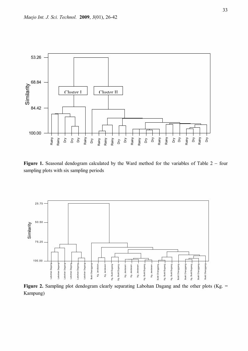
Cluster analysis is a common method applied in unsupervised pattern recognition [1,32]. It was applied in this work to search for clusters due to different sampling seasons or different sampling sites by using water quality variables or features. The agglomerative hierarchical cluster analysis according to Ward’s methods [21,23] using squared Euclidean distances was applied to detect multivariate similarities between sampling sites in different sampling plots at different sampling days. From Figure 1 it is observed that the separation between clusters 1 and 2 does not show a significant impact due to seasonal change. Differences in the feature values (water quality parameters) are probably due to seasonal changes distributed over the whole area of sampling plots. They do not, however, form the basis for the separation observed in the objects (sampling sites).

On the other hand, Figure 2 shows that if the separation is grouped according to sampling plots, it shows clear discrimination of Labohan Dagang and the other sites. It can be seen that Labohan Dagang (Group 1) sampling plot at similarity level 75.25 (dashed line in Figure 2) is very different from the others. In this study the other sampling plots that merge at similarity level 75.25 (Bukit Changgang, Kampung Jenderam and Kampung Bukit Dugang) forms a single group (Group 2).


32

Table 3. Physicochemical properties of water at various sampling sites Variable 1 2 3 4 5 6 7 8 9 10 11 12 13 14 15 16

Sampling site pH Temp. Cond. TSS DO BOD COD AN PO4 NO3 SO4 Pb Cd Fe Zn Cu

(C) (µS/cm) (mg/L) (mg/L) (mg/L) (mg/L) (mg/L) (mg/L) (mg/L) (mg/L) (mg/L) (mg/L) (mg/L) (mg/L) (mg/L)

Kampung Bukit Dugang (26/12/2001) 5.8 30.0 69 65.4 3.0 5.44 21 1.57 0.16 3.1 0.8 0.54 0.01 2.8 0.04 32.56

Kampung Jenderam (26/12/2001) 3.5 27.0 126 2.8 1.5 3.74 18 1.57 0.14 0.9 6.6 0.26 0.01 2.2 0.08 2.01

Bukit Changgang (26/12/2001) 5.9 28.0 67 186.3 4.7 6.20 9 1.32 0.08 1.3 0.6 0.37 0.01 0.09 0.02 2.46

Labohan Dagang (26/12/2001) 5.8 29.0 96 815.3 3.6 5.44 45 0.57 0.04 6.3 138.9 0.55 0.02 2.2 0.08 2



Bukit Changgang (10/01/2002) 5.3 29.6 189 283.7 4.2 1.32 24 1.34 0.11 2.8 20.6 2.73 0.14 3.8 2.24 3.31

Labohan Dagang (10/01/2002) 5.6 30.0 175 746.9 1.7 0.68 10 0.87 0.03 5.7 102.6 1.11 0.16 0.38 1.67 2.05



Bukit Changgang (19/02/2002) 5.4 32.9 215 119.9 5.0 1.17 2 1.71 0.12 3.9 25.0 2.57 0.13 5.87 1.96 1.44

Labohan Dagang (19/02/2002) 5.5 30.5 290 724.3 0.6 0.01 27 1.44 0.01 3.9 44.0 1.79 0.13 0.62 2.23 1.62



Bukit Changgang (3/03/2002) 4.2 29.2 153 147.6 1.1 1.14 0 1.84 0.01 1.4 27.0 3.57 0.69 3.47 3.42 0.26

Labohan Dagang (3/03/2002) 5.1 29.1 74 951.4 3.4 0.29 10 2.04 0.01 1.1 31.0 2.84 0.18 0.16 5.89 0.12


Kampung Jenderam (13/04/2002) 5.2 29.6 106 0.2 2.1 0.43 1 1.89 0.26 1 1.0 2.58 0.18 1.18 6.87 0.13

Bukit Changgang (13/04/2002) 5.9 29.8 132 123.5 3.6 0.99 2 1.89 0.01 1.5 32.0 2.39 0.43 3.21 3.14 0.03

Labohan Dagang (13/04/2002) 5.1 29.9 92 795.7 4.0 0.67 26 1.99 0.01 1.2 29.0 3.81 0.1 0.14 7.21 0.18



Bukit Changgang (15/05/2002) 6.3 32.4 104 85.3 5.1 1.21 1 1.23 0.00 1.2 18.0 5.54 0.6 3.49 4.39 0.22

Labohan Dagang (15/05/2002) 4.6 30.3 263 734.7 4.7 0.43 7 2.41 0.02 1.5 63.0 3.79 0.01 0.15 1.79 0.43


33

Rai

ny

Rai

ny Dry

Dry Dry

Rai

ny

Dry

Rai

ny

Rai

ny

Rai

ny

Dry Dry

Rai

ny

Rai

ny Dry Dry

Rai

ny

Rai

ny

Dry Dry

Rai

ny Dry

Rai

ny Dry

100.00

84.42

68.84

53.26

Sim

ilarit

y

Figure 1. Seasonal dendogram calculated by the Ward method for the variables of Table 2 four sampling plots with six sampling periods

Buk

it C

hang

gang

Buk

it C

hang

gang

Kg.

Buk

it D

ugan

g

Buk

it C

hang

gang

Buk

it C

hang

gang

Kg.

Buk

it D

ugan

g

Kg.

Buk

it D

ugan

g

Buk

it C

hang

gang

Kg.

Jen

dera

m

Kg.

Buk

it D

ugan

g

Kg.

Jen

dera

m

Kg.

Jen

dera

m

Kg.

Jen

dera

m

Kg.

Buk

it D

ugan

g

Kg.

Buk

it D

ugan

g

Kg.

Jen

dera

m

Kg.

Jen

dera

m

Buk

it C

hang

gang

Labo

han

Dag

ang

2 5.75

5 0.50

7 5.25

100.00

Sim

ilarit

y

Labo

han

Dag

ang

Labo

han

Dag

ang

Labo

han

Dag

ang

Labo

han

Dag

ang

Labo

han

Dag

ang

Figure 2. Sampling plot dendogram clearly separating Labohan Dagang and the other plots (Kg. = Kampung)

Cluster I Cluster II


34

The two groups of samples from plot 4 (Group 1) and plots 1, 2 and 3 (Group 2) join at a lower level of similarity in the sampling plot dendogram (Figure 2) compared to the seasonal dendogram (Figure 1). This demonstrates that from a hierarchical point of view the difference between the two separated groups (1 and 2) is larger in the sampling plot dendogram (Figure 2) compared to the seasonal dendogram (Figure 1). This is an indication that separation of sampling plots should be used as a significant factor in forming the basis for choosing sampling sites in order to study the effects of palm oil plantation on water quality. Searching for seasonal dependency based on the conventionally chosen sampling sites is consequently an ineffective exercise which involves high cost and much sampling time being wasted. Principal component analysis

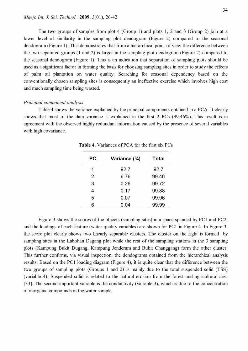
Table 4 shows the variance explained by the principal components obtained in a PCA. It clearly shows that most of the data variance is explained in the first 2 PCs (99.46%). This result is in agreement with the observed highly redundant information caused by the presence of several variables with high covariance.

Table 4. Variances of PCA for the first six PCs

PC Variance (%) Total

1 92.7 92.7 2 6.76 99.46 3 0.26 99.72 4 0.17 99.88 5 0.07 99.96 6 0.04 99.99

Figure 3 shows the scores of the objects (sampling sites) in a space spanned by PC1 and PC2,

and the loadings of each feature (water quality variables) are shown for PC1 in Figure 4. In Figure 3, the score plot clearly shows two linearly separable clusters. The cluster on the right is formed by sampling sites in the Labohan Dagang plot while the rest of the sampling stations in the 3 sampling plots (Kampung Bukit Dugang, Kampung Jenderam and Bukit Changgang) form the other cluster. This further confirms, via visual inspection, the dendograms obtained from the hierarchical analysis results. Based on the PC1 loading diagram (Figure 4), it is quite clear that the difference between the two groups of sampling plots (Groups 1 and 2) is mainly due to the total suspended solid (TSS) (variable 4). Suspended solid is related to the natural erosion from the forest and agricultural area [33]. The second important variable is the conductivity (variable 3), which is due to the concentration of inorganic compounds in the water sample.


35

Bukit Changgang

Kg. Bukit DugangBukit Changgang

Kg. Bukit DugangBukit Changgang

Kg. Bukit DugangKg. Bukit DugangKg. Bukit Dugang

Kg. Jenderam

Kg. Jenderam Kg. JenderamKg. Jenderam

Bukit Changgang

Kg. Jenderam

Kg. Jenderam

Bukit Changgang

Kg. Bukit Dugang

Labohan Dagang

Labohan Dagang

Labohan Dagang

Labohan Dagang

Labohan Dagang

Labohan DagangBukit Changgang

-200

-150

-100

-50

0

50

100

150

200

250

300

0 100 200 300 400 500 600 700 800 900 1000

PC1

PC2

Figure 3. Principal component analysis (PCA) for four sampling plots (with six sampling periods)

Figure 4. Plot of PC1 loadings


36

Based on these results, it would be rather inappropriate to maintain the existing sampling sites, which were chosen based on economic reasons, if we are interested to study why certain areas exhibit high TSS. Sampling sites within group 2, for example, are rather redundant in this case. For further studies concerning the phenomena of high TSS, sampling sites within the plot of Labohan Dagang should be increased. Design of experiments: Factorial design

If we are interested to study the interaction between two factors, such as the seasonal and sampling site factors as discussed in this work, we can use statistical methods classified under factorial design to do this. With the method, we can evaluate the effects of two or more factors simultaneously [34]. In this case, we try to interpret the results by testing whether there is an interaction effect between factor I (sampling plots) and factor II (weather condition). If the interaction effect between the factors is significant, one must be cautious in interpreting the phenomena. On the other hand, if the interaction effect is not significant, the focus of interpretation should be based on the potential differences between sampling plots (factor I) and weather condition (factor II).

Table 6 tabulates the ANOVA results obtained in testing for differences between two sampling plots (factor I): A (Labohan Dagang) and B (Kampung Jenderam, Bukit Changgang and Kampung Bukit Dugang). The decision rule in this test is to reject the null hypothesis if the calculated F value exceeds 5.32, which is the upper-tail critical value from the F distribution with 1 degree of freedom in the numerator and 18 degrees of freedom in the denominator. Because F = 372.65 > Fu = 5.32, and because the p-value = 5.38E-08 < 0.05, we reject the null hypothesis, and conclude that there is evidence of a difference between the two sampling plots in terms of the average amount of TSS. For sampling plot A, more TSS was observed (an average of 854.13 mg/L) compared to sampling plot B (an average of 138.67 mg/L).

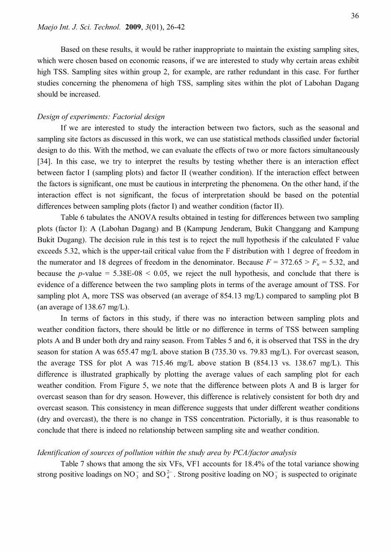
In terms of factors in this study, if there was no interaction between sampling plots and weather condition factors, there should be little or no difference in terms of TSS between sampling plots A and B under both dry and rainy season. From Tables 5 and 6, it is observed that TSS in the dry season for station A was 655.47 mg/L above station B (735.30 vs. 79.83 mg/L). For overcast season, the average TSS for plot A was 715.46 mg/L above station B (854.13 vs. 138.67 mg/L). This difference is illustrated graphically by plotting the average values of each sampling plot for each weather condition. From Figure 5, we note that the difference between plots A and B is larger for overcast season than for dry season. However, this difference is relatively consistent for both dry and overcast season. This consistency in mean difference suggests that under different weather conditions (dry and overcast), the there is no change in TSS concentration. Pictorially, it is thus reasonable to conclude that there is indeed no relationship between sampling site and weather condition.

Identification of sources of pollution within the study area by PCA/factor analysis

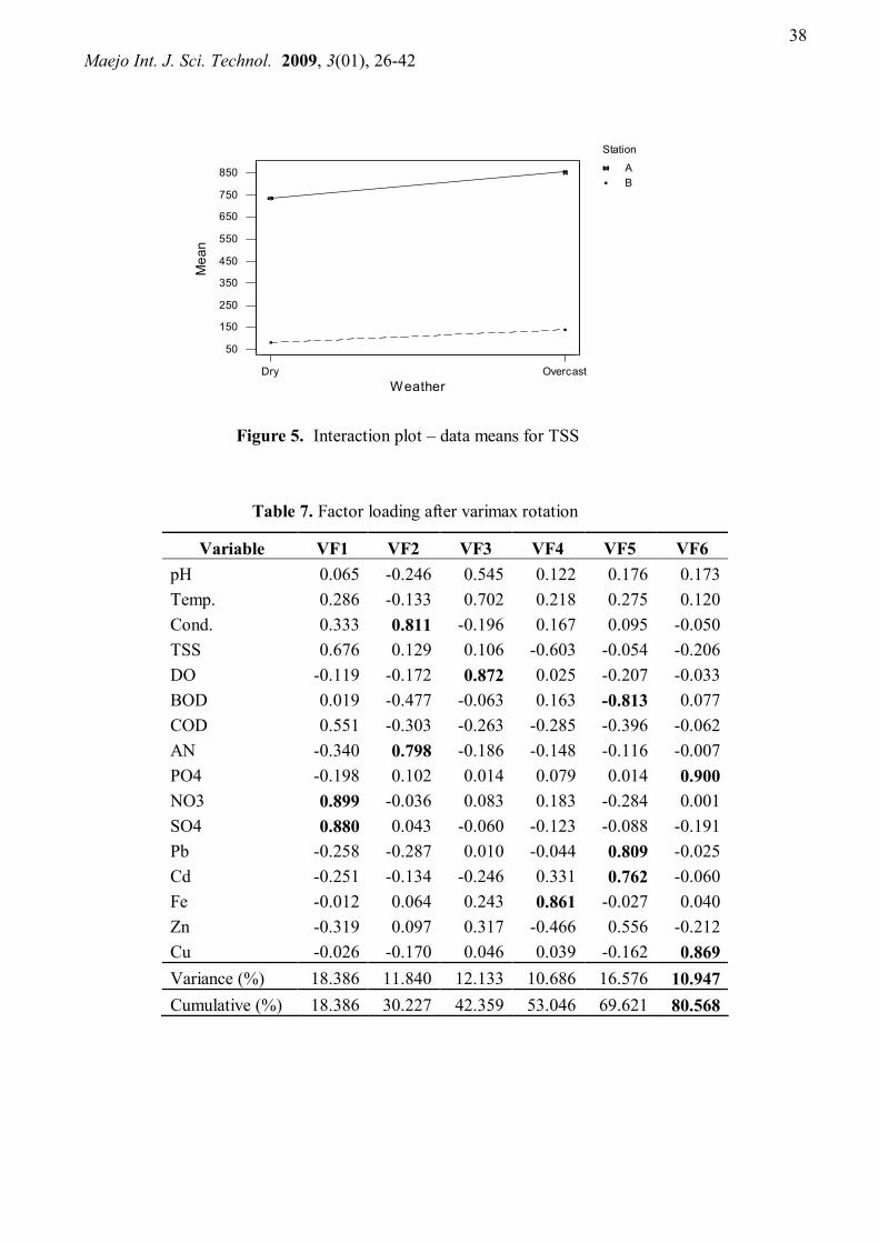
Table 7 shows that among the six VFs, VF1 accounts for 18.4% of the total variance showing strong positive loadings on NO

3 and SO 24 . Strong positive loading on NO

3 is suspected to originate


37

Table 5. Summary of TSS average and variance for plots A and B measured under two different weather conditions

Table 6. ANOVA results in testing the difference in TSS measurements for sampling plots A and B

Source of Variation SS df MS F p-value F crit

Sample 1409594 1 1409594 372.6449 5.38E-08 5.317655 Columns 23674.08 1 23674.08 6.25856 0.036844 5.317655 Interaction 2700 1 2700 0.713781 0.422737 5.317655 Within 30261.38 8 3782.673 Total 1466229 11

from agricultural fields [11] where irrigated horticultural crops are grown and the use of inorganic fertilisers (usually as ammonium nitrate) is rather frequent. This practice could also explain the high levels of ammonia, but this pollutant may also originate from decomposition of nitrogen-containing organic compounds via degradation process of organic matters [35] such as proteins and urea occurring in municipal wastewater discharges. The presence of SO 2

4 may be attributed to the acid sulphate soils along the river banks.

Summary Overcast Dry Total A

Count 3 3 6 Sum 2562.4 2205.9 4768.3 Average 854.1333 735.3 794.7167 Variance 7191.643 127.96 7164.25

B Count 3 3 6 Sum 416 239.5 655.5 Average 138.6667 79.83333 109.25 Variance 3853.243 3957.843 4162.843

Total Count 6 6 Sum 2978.4 2445.4 Average 496.4 407.5667 Variance 157985.7 130525.3


38

A B

OvercastDry

850

750

650

550

450

350

250

150

50

Weather

Station

Mea

n

Figure 5. Interaction plot – data means for TSS

Table 7. Factor loading after varimax rotation

Variable VF1 VF2 VF3 VF4 VF5 VF6

pH 0.065 -0.246 0.545 0.122 0.176 0.173 Temp. 0.286 -0.133 0.702 0.218 0.275 0.120 Cond. 0.333 0.811 -0.196 0.167 0.095 -0.050 TSS 0.676 0.129 0.106 -0.603 -0.054 -0.206 DO -0.119 -0.172 0.872 0.025 -0.207 -0.033 BOD 0.019 -0.477 -0.063 0.163 -0.813 0.077 COD 0.551 -0.303 -0.263 -0.285 -0.396 -0.062 AN -0.340 0.798 -0.186 -0.148 -0.116 -0.007 PO4 -0.198 0.102 0.014 0.079 0.014 0.900 NO3 0.899 -0.036 0.083 0.183 -0.284 0.001 SO4 0.880 0.043 -0.060 -0.123 -0.088 -0.191 Pb -0.258 -0.287 0.010 -0.044 0.809 -0.025 Cd -0.251 -0.134 -0.246 0.331 0.762 -0.060 Fe -0.012 0.064 0.243 0.861 -0.027 0.040 Zn -0.319 0.097 0.317 -0.466 0.556 -0.212 Cu -0.026 -0.170 0.046 0.039 -0.162 0.869 Variance (%) 18.386 11.840 12.133 10.686 16.576 10.947 Cumulative (%) 18.386 30.227 42.359 53.046 69.621 80.568


39

VF2, VF3 and VF4 account for 11.8%, 12.1% and 10.7% of the total variance and show strong positive loadings on AN, conductivity, DO and Fe content. The presence of AN is related to the influence of domestic waste and agricultural runoff [36-38] in their study, found that higher nitrogen levels were detected in agricultural waters, where fertilisers, manure and pesticides had been applied. Strong positive loadings on conductivity and DO could be explained by considering the chemical components of various anthropogenic activities which constitute point source pollution especially from industrial, domestic, commercial and agricultural runoff areas located at Hulu Langat, Cheras and Kajang districts. The presence of Fe basically represents the metal group originating from industrial effluents.

VF5 accounts for 16.6% of the total variance and shows strong positive loading on Pb and Cd and strong negative loading on BOD. Factories along the river bank may have contributed to the presence of Pb and Cd. VF6 accounts for 11% of the total variance and shows strong positive loading on PO 3

4 and Cu. The presence of PO 34 is most probably due to agricultural runoff such as livestock

waste and fertilisers [39], industrial effluents, municipal sewage and existing sewage treatment plants because PO 3

4 is an important component of detergents [11].

Conclusions

This study has demonstrated that simple chemometric treatments are able to draw out from raw historical data information that would enable us to more effectively determine the “right” sampling sites for a particular objective, in order to reduce cost and time. In the case of the data obtained from the study, in order to determine the effects of palm oil plantation on water quality in the future, the researcher can determine the sampling sites in a more effective manner, relating the objective of the study to the type of sites to be chosen for sampling purpose.

Based on the original sampling sites, which were determined by economic reasons, it was found that the seasonal factor does not form a good basis of separation. Sampling sites and plots do not form reasonable clusters when weather condition is used as the factor. Thus, for the purpose of studying how seasonal change affects the water quality of this stretch of the basin, retaining the original sampling sites would prove ineffective. The sampling sites chosen in plots 1, 2 and 3 prove to be redundant for this purpose and should be reassessed. On the other hand, the separation of sampling plots due to suspended solid and conductivity, if these were historically available for the studied area, should motivate one to further study this phenomena. In designing sampling strategy for this purpose, TSS and conductivity must be considered as significant factors for reassessment to avoid redundant and unsuitable sampling sites.

This is just one simple example of the use of historical data and chemometric methods in determining new directions of sampling strategy, which results in the saving of sampling time and cost. Annual or even monthly reassessment of sampling sites based on this strategy may prove to be highly cost and time effective as well as direct research into new areas of study. The application of cluster


40

analysis, followed by principal component analysis as a classification method as demonstrated in this study, would help tremendously in future river pollution monitoring program.

Acknowledgements

The authors thank the Institute of Environment and Development (LESTARI), University Kebangsaan Malaysia for providing secondary water quality data, and Chemistry Department, Faculty of Science, University of Malaya for supporting this work.

References

1. J. W. Einax, D. Truckenbrodt, and O. Ampe, “River pollution data interpreted by means of methods”, Microchem. J., 1998, 58, 315-324.

2. V. Simeonov, J. W. Einax, I. Stanimirova, and J. Kraft, ”Envirometric modeling and interpretation of river water monitoring data”, Anal. Bioanal. Chem., 2002, 374, 898-905.

3. D. I. Massart, B.G. M. Vandeginste, L. M. C. Buydens, S. De Long, P. J. Ewi, and J. Smeyers-Verbeke, “Handbook of Chemometric and Qualimetrics, Part A”, Elsevier, Amsterdam, 1997.

4. W. A. Khalil, A. Oonetillke, S. Kokot, and S. Carrol, “Use of s methods and multicriteria decision-making for site selection for sustainable on-site sewage effluent disposal”, Anal. Chim. Acta , 2003, 506, 41-56.

5. O. Abollina, M. Aceto, C. L. Gioia, C. Sarzanini, and E. Mentasti, “Spatial and seasonal variations of major, minor and trace elements in Antartic seawater. Investigation of variable and site correlations”, Adv. Environ. Res., 2001, 6, 29-43.

6. A. K. Meng and I. H. Suffet, “A procedure for correlation of chemical and sensory data in drinking water samples by principal component factor analysis”, Environ. Sci. Technol., 1997, 31, 337-345.

7. C. Mendiguchia, C. Moreno, D. M. Galindo-Riano, and M. Arcia-Vargas, “Using chemometric tools to assess anthropogenic effects in river water. A case study: Guadalquivir River (Spain)”, Anal. Chim. Acta, 2004, 515, 143-149.

8. D. Brodnjak-Voncina, D. Dobcnik, M. Novic, and J. Zupan, “Characterization of the quality of river water” Anal. Chim. Acta, 2002, 462, 87-100.

9. E. Marengo, M. C. Gennaro, D. Giacosa, C. Abrigo, G. Saini, and M. T. Avignone, “How s can helpfully assist in evaluating environmental data lagoon water”, Anal. Chim. Acta, 1995, 317, 53-63.

10. T. Kowalkowski, R. Zbytniewski, J. Szpejna, and B. Buszewski, “Application of chemometrics in river water classification” Water Res., 2006, 40, 744-752.

11. M. Vega, R. Pardo, E. Barrado, and L. Deban, “Assessment of seasonal and polluting effects on the quality of river water by exploratory data analysis”, Water Res., 1998, 32, 3581-3592.


41

12. S. Suresh and F. Kazama, “Assessment of surface water quality using multivariate statistical techniques: A case study of the Fuji River basin, Japan”, Environ. Model. Softw., 2007, 22, 464-475.

13. B. Helena, R. Pardo, M. Vega, E. Barrado, J. M. Fernandez, and L. Fernandez, “Temporal evaluation of groundwater composition in an alluvial aquifer (Pisuerga River, Spain) by principal component analysis”, Water Res., 2000, 34, 807-816.

14. K. P. Singh, A. Malik, D. Mohan, and S. Sinha, “Multivariate statistical techniques for the evaluation of spatial and temporal variations in water quality of Gomti River (India)_a case study”, Water Res., 2004, 38, 3980-3992.

15. S. D. Brown, T. B. Blank, S. T. Sum, and L. G. Weyer, “Chemometrics” Anal. Chem., 1994, 66, 315R-359R.

16. S. D. Brown, S. T. Sum, and F. Despagne, “Chemometrics”, Anal. Chem., 1996, 68, 21R-61R.

17. W. D. Alberto, D. M. D. Pilar, A. M. Valeria, P. S. Fabiana, H. A. Cecilia, and B. M. D. L. Angeles, “Pattern recognition techniques for the evaluation of spatial and temporal variations in water quality. A case study: Squia River Basin (Cordoba-Argentina)”, Water Res., 2001, 35, 2881-2894.

18. P. R. Kannel, S. Lee, S. R. Kanel, and S. P. Khan, “ Chemometric application in classification and assessment of monitoring locations of an urban river system”, Anal. Chim. Acta, 2007, 582, 390-399.

19. A. Qadir, R. N. Malik, and S. Z. Husain, “Spatio-temporal variations in water quality of Nullah Aik-tributary of the River Chenab, Pakistan”, Environ. Monit. Assess., 2008, 140, 53-49.

20. M. Kent and P. Coker, “Vegetation Description and Analysis: A Practical Approach”, Belhaven, London, 1992.

21. D. L. Massart and L. Kaufman, “The Interpretation of Analytical Data by the Use of Cluster Analysis”, Wiley, New York, 1983.

22. J. E. McKenna Jr., “An enhanced cluster analysis program with bootstrap significance testing for ecological community analysis’, Environ. Model. Softw., 2003, 18, 205-220.

23. P. Willet, “ Similarity and Clustering in Chemical Information Systems”, Wiley, New York, 1987.

24. M. J. Adams, in “The Principles of Multivariate Data Analysis” (Ed. P. R. Ashurst and M. J. Dennis), Blackie Academic & Professional, London, 1998.

25. M. Otto, “Multivariate Methods” in “Analytical Chemistry” (Ed. R. Kellner, J. M. Mermet, M. Otto, and H. M. Widmer), Wiley-VCH, Wenheim, 1998.

26. M. Forina, C. Armanino, and V. Raggio, “ Clustering with dendograms on interpretation variables”, Anal. Chim. Acta, 2002, 454, 13-19.


42

27. K. P. Singh, A. Malik, and S. Sinha, ”Water quality assessment and apportionment of pollution sources of Gomti River (India) using multivariate statistical techniques: A case study”, Anal. Chim. Acta, 2005, 35, 3581-3592.

28. J. O. Kim and C. W. Mueller, “Introduction to Factor Analysis: What It Is and How to Do It”, Sage University Press, Newbury Park, 1987.

29. R. Mead, R. N. Curnow, and A. M. Hasted, “Statistical Methods in Agriculture and Experimental Biology”, 2nd Edn., Chapman & Hall, London, 1993.

30. H. J. Brightmen, “Data Analysis in Plain English with Microsoft Excel”, Duxbury Press, Singapore, 1999.

31. C. W. Liu, K. H. Lin, and Y. M. Kuo, “Application of factor analysis in the assessment of groundwater quality in a blackfoot disease area in Taiwan”, Sci. Total Environ., 2003, 313, 77-89.

32. R. G. Brereton, “Data Analysis for the Laboratory and Chemical Plant”, John Wiley & Son, West Sussex, 2002.

33. W. M. Muhiyuddin, W. Ibrahim, I. Komoo, and J. J. Pereira, “Relationship between physical degradation and land cover changes in the Langat Basin (in Malay)”, Proceedings of the 1999 Langat Basin Research Symposium, LESTARI, Universiti Kebangsaan Malaysia, Bangi, Malaysia, 1999, pp. 126–134.

34. M. D. Levine, P. P. Ramsey, and R. K. Smidt, “Applied Statistics for Engineers and Scientists: Using Microsoft Excel and MINITAB”, Int. Edn., Prentice-Hall, New Jersey, 2001.

35. U.S. Geological Survey, “Water quality in the upper Anacostica River, Maryland: Continuous and discrete monitoring with simulations to estimate concentrations and yields, 2003-05”, Scientific Investigation Report, 2007.

36. D. S. Fisher, J. L. Steiner, D. M. Endale, J. A. Stuedemann, H. H. Schomberg, and S. R. Wilkinson, “The relationship of land use practices to surface water quality in the upper Oconee watershed of Georgia”, Forest Ecol. Manage., 2000, 128, 39-48.

37. L. L. Osborne and M. J. Wiley, “Empirical relationships between land use/cover and stream water quality in an agricultural watershed”, J. Environ. Manage., 1988, 26, 9-27.

38. A. M. McFarland and S .L. Hauck, “Relating agricultural land uses to in-stream storm water quality”, J. Environ. Qual., 1999, 28, 836-844.

39. O. Buck, D. K. Niyogi, and C. R. Townsend, “Scale-dependence of land use effects on water quality of streams in agricultural catchments”, Environ. Pollut., 2003, 130, 287-299.

© 2009 by Maejo University, San Sai, Chiang Mai, 50290 Thailand. Reproduction is permitted for noncommercial purposes.

maejo int. j. sci. technol. maejo international journal of science and ... · chemometrics can be...

Documents