arX

iv:1

501.

0339

3v5

[qu

ant-

ph]

2 N

ov 2

015

Macroscopic Observability of Spinorial Sign Changes: A Reply to Gill

Joy Christian∗

Einstein Centre for Local-Realistic Physics, 15 Thackley End, Oxford OX2 6LB, United Kingdom

In a recent paper Richard Gill has criticized an experimental proposal published in a journal ofphysics which describes how to detect a macroscopic signature of spinorial sign changes. Here I pointout that Gill’s worries stem from his own elementary algebraic and conceptual mistakes, and presentseveral event-by-event numerical simulations which bring out his mistakes by explicit computations.

In a recent paper a mechanical experiment has been proposed to test possible macroscopic observability of spinorialsign changes under 2π rotations [1]. The proposed experiment is a variant of the local model for the spin-1/2 particlesconsidered by Bell [2], which was later further developed by Peres providing pedagogical details [3][4]. Our experimentdiffers, however, from the one considered by Bell and Peres in one important respect. It involves measurements of theactual spin angular momenta of two fragments of an exploding bomb rather than their normalized spin values, ±1.

It is well known that angular momenta are best described, not by ordinary polar vectors, but by pseudo-vectors, orbivectors, that change sign upon reflection [4][5]. One only has to compare a spinning object, like a barber’s pole, withits image in a mirror to appreciate this elementary fact. The mirror image of a polar vector representing the spinningobject is not the polar vector that represents the mirror image of the spinning object. In fact it is the negative ofthe polar vector that does the job. Therefore the spin angular momenta L(a, λ) in the theoretical analysis of theexperiment proposed in the paper [1] have been represented by bivectors using the powerful language of geometricalgebra [6]. They can be expressed in terms of the bivector basis (which are graded basis) satisfying the sub-algebra

Lµ(λ)Lν(λ) = − gµν −∑

ρ

ǫµνρ Lρ(λ) , (1)

where λ = ± 1 represents a choice of orientation of a unit 3-sphere [1]. This brings us to the first of several elementarymistakes made by Gill. In his paper [7] he claims that, from the above equation, using Lµ(λ = −1) = −Lµ(λ = +1),

Lµ(λ = +1)Lν(λ = +1) − Lµ(λ = −1)Lν(λ = −1) = −∑

ρ

ǫµνρ Lρ(λ = +1) +∑

ρ

ǫµνρ Lρ(λ = −1) (2)

implies 0 = −2∑

ρ

ǫµνρ Lρ(λ = +1) = +2∑

ρ

ǫµνρ Lρ(λ = −1), (3)

which in turn implies Lρ(λ = +1) = Lρ(λ = −1) = 0 . (4)

It is not difficult to see, however, that this claim is manifestly false. Gill’s mistake here is to miss the summation overthe index ρ. And since the basis elements Lρ(λ = +1) and Lρ(λ = −1) do not vanish in general, contrary to his claimneither the spin angular momentum L(a, λ) about the direction a nor the spin angular momentum L(b, λ) about thedirection b vanish in general. Only the spin angular momentum L(a × b, λ) about the mutually orthogonal directiona× b vanish, as in Eq. (110) of the paper [1]. This is of course consistent with the physical fact that there is no thirdfragment of the bomb spinning about the direction a× b exclusive (as well as orthogonal) to both directions a andb. To see that only the spin angular momentum L(a× b, λ) about the direction a× b vanishes, all one has to do isto contract Eq. (1) above with the vector components aµ and bν , on both sides, and then follow through the steps inEqs. (2) and (3). It is also crucial to appreciate that the spin angular momenta L(s, λ) (i.e., the bivectors) trace outan su(2) 2-sphere within the group manifold SU(2) ∼ S3, not a round S2 within IR3 as Gill has incorrectly assumed.

Unfortunately the conceptual mistakes made by Gill are even more serious than the above elementary mathematicalmistakes [7][8]. As already noted, what are supposed to be measured in the proposed experiment are the spin angularmomenta L(a, λ) and L(b, λ) themselves, not their normalized spin values ±1 about some directions a and b, where

L(a, λ) ≡ A(a, λ) ≡ λ(ex ∧ ey ∧ ez) · a = ±1 spin about a (5)

and L(b, λ) ≡ B(b, λ) ≡ λ(ex ∧ ey ∧ ez) · b = ±1 spin about b . (6)

This is in sharp contrast to what are measured as dynamical variables in the model considered by Bell and Peres [4].

∗Electronic address: jjc@alum.bu.edu

2

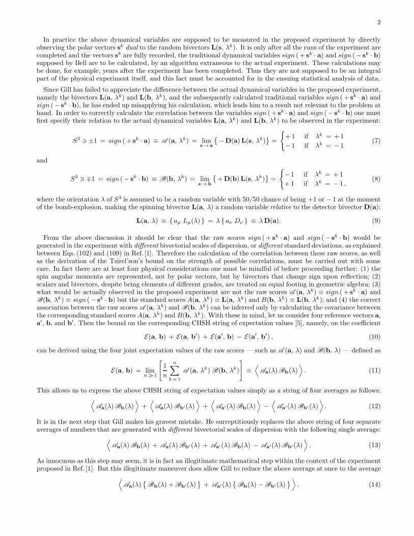
In practice the above dynamical variables are supposed to be measured in the proposed experiment by directlyobserving the polar vectors sk dual to the random bivectors L(s, λk). It is only after all the runs of the experiment arecompleted and the vectors sk are fully recorded, the traditional dynamical variables sign (+ sk · a) and sign (− sk · b)supposed by Bell are to be calculated, by an algorithm extraneous to the actual experiment. These calculations maybe done, for example, years after the experiment has been completed. Thus they are not supposed to be an integralpart of the physical experiment itself, and this fact must be accounted for in the ensuing statistical analysis of data.

Since Gill has failed to appreciate the difference between the actual dynamical variables in the proposed experiment,namely the bivectors L(a, λk) and L(b, λk), and the subsequently calculated traditional variables sign (+ sk · a) andsign (− sk · b), he has ended up misapplying his calculation, which leads him to a result not relevant to the problem athand. In order to correctly calculate the correlation between the variables sign (+ sk · a) and sign (− sk · b) one mustfirst specify their relation to the actual dynamical variables L(a, λk) and L(b, λk) to be observed in the experiment:

S3 ∋ ±1 = sign (+ sk · a) ≡ A (a, λk) = lims→ a

{

−D(a)L(s, λk)}

=

{

+1 if λk = +1

− 1 if λk = − 1(7)

and

S3 ∋ ∓1 = sign (− sk · b) ≡ B(b, λk) = lims→b

{

+D(b)L(s, λk)}

=

{

− 1 if λk = +1

+1 if λk = − 1 ,(8)

where the orientation λ of S3 is assumed to be a random variable with 50/50 chance of being +1 or − 1 at the momentof the bomb-explosion, making the spinning bivector L(a, λ) a random variable relative to the detector bivector D(a):

L(a, λ) ≡ { aµ Lµ(λ) } = λ { aν Dν } ≡ λD(a). (9)

From the above discussion it should be clear that the raw scores sign (+ sk · a) and sign (− sk · b) would begenerated in the experiment with different bivectorial scales of dispersion, or different standard deviations, as explainedbetween Eqs. (102) and (109) in Ref. [1]. Therefore the calculation of the correlation between these raw scores, as wellas the derivation of the Tsirel’son’s bound on the strength of possible correlations, must be carried out with somecare. In fact there are at least four physical considerations one must be mindful of before proceeding further: (1) thespin angular momenta are represented, not by polar vectors, but by bivectors that change sign upon reflection; (2)scalars and bivectors, despite being elements of different grades, are treated on equal footing in geometric algebra; (3)what would be actually observed in the proposed experiment are not the raw scores A (a, λk) ≡ sign (+ sk · a) andB(b, λk) ≡ sign (− sk · b) but the standard scores A(a, λk) ≡ L(a, λk) and B(b, λk) ≡ L(b, λk); and (4) the correctassociation between the raw scores A (a, λk) and B(b, λk) can be inferred only by calculating the covariance betweenthe corresponding standard scores A(a, λk) and B(b, λk). With these in mind, let us consider four reference vectors a,a′, b, and b′. Then the bound on the corresponding CHSH string of expectation values [5], namely, on the coefficient

E(a, b) + E(a, b′) + E(a′, b) − E(a′, b′) , (10)

can be derived using the four joint expectation values of the raw scores — such as A (a, λ) and B(b, λ) — defined as

E(a, b) = limn≫ 1

[

1

n

n∑

k=1

A (a, λk) B(b, λk)

]

≡⟨

Aa(λ)Bb(λ)⟩

. (11)

This allows us to express the above CHSH string of expectation values simply as a string of four averages as follows:⟨

Aa(λ)Bb(λ)⟩

+⟨

Aa(λ)Bb′ (λ)⟩

+⟨

Aa′(λ)Bb(λ)⟩

−⟨

Aa′(λ)Bb′ (λ)⟩

. (12)

It is in the next step that Gill makes his gravest mistake. He surreptitiously replaces the above string of four separateaverages of numbers that are generated with different bivectorial scales of dispersion with the following single average:

⟨

Aa(λ)Bb(λ) + Aa(λ)Bb′ (λ) + Aa′(λ)Bb(λ) − Aa′(λ)Bb′(λ)⟩

. (13)

As innocuous as this step may seem, it is in fact an illegitimate mathematical step within the context of the experimentproposed in Ref. [1]. But this illegitimate maneuver does allow Gill to reduce the above average at once to the average

⟨

Aa(λ){

Bb(λ) + Bb′(λ)}

+ Aa′(λ){

Bb(λ)− Bb′(λ)}

⟩

. (14)

3

And since Bb(λ) = ±1, if |Bb(λ) + Bb′(λ)| = 2, then |Bb(λ) − Bb′(λ)| = 0, and vice versa. Consequently, usingAa(λ) = ±1, it is easy to conclude that the absolute value of the above average cannot exceed 2, as Gill has concluded.

As compelling as this conclusion by Gill may seem at first sight, it is entirely false. It is based on his illegitimate andcareless maneuver of replacing the string of four separate averages of random variables (12) with a single average (13).Such a move is justified on mathematical grounds only if all four random variables Aa(λ), Bb(λ), Aa′(λ), and Bb′(λ)are on equal statistical and geometrical footings. But as we noted earlier, each one of these variables is generatedwith a different bivectorial scale of dispersion, or a different standard deviation, as explained between equations (102)and (109) in Ref. [1]. Therefore the theoretical prediction of the correlation (11) between these raw scores, as well asthe theoretical derivation of the Tsirel’son’s bound on the strength of possible correlations, must proceed as follows.

Since the correct association between the raw scores A (a, λ) and B(b, λ) can be inferred only by calculating thecovariance between the corresponding standardized variables A(a, λ) and B(b, λ) as calculated in Ref. [1], namely

Aa(λ) ≡ A(a, λ) ≡ L(a, λ) (15)

and Bb(λ) ≡ B(b, λ) ≡ L(b, λ) , (16)

the correlation between the raw scores A (a, λ) and B(b, λ) must be obtained by evaluating their product moment

E(a, b) = limn≫ 1

[

1

n

n∑

k=1

A(a, λk) B(b, λk)

]

. (17)

The numerical value of this coefficient is then necessarily equal to the value of the correlation calculated by Eq. (11).

Using the above expression for E(a, b) the string of expectation values (10) can now be rewritten as a single averagein terms of the standard scores Aa(λ) and Bb(λ), because now they are on equal statistical and geometrical footings:

limn≫ 1

[

1

n

n∑

k=1

{

Aa(λk)Bb(λ

k) + Aa(λk)Bb′(λk) + Aa′(λk)Bb(λ

k) − Aa′(λk)Bb′(λk)}

]

. (18)

But since Aa(λ) ≡ L(a, λ) and Bb(λ) ≡ L(b, λ) are two independent equatorial points of S3, we can take them tobelong to two disconnected “sections” of S3 [i.e., two disconnected su(2) 2-spheres within S3 ∼ SU(2)], satisfying

[An(λ), Bn′(λ) ] = 0 ∀ n and n′ ∈ IR3, (19)

which is equivalent to anticipating a null outcome along the direction n× n′ exclusive to both n and n′. If we nowsquare the integrand of equation (18), use the above commutation relations, and use the fact that all unit bivectorssquare to −1, then the absolute value of the Bell-CHSH string (10) leads to the following variance inequality [5]:

|E(a, b) + E(a, b′) + E(a′, b) − E(a′, b′)| 6

√

√

√

√ limn≫ 1

[

1

n

n∑

k=1

{

4 + 4T aa′(λk)Tb′ b(λk)}

]

, (20)

where the classical commutators

T a a′(λ) :=1

2[Aa(λ), Aa′(λ)] = −Aa×a′(λ) (21)

and

Tb′ b(λ) :=1

2[Bb′(λ), Bb(λ)] = −Bb′×b(λ) (22)

are the geometric measures of the torsion within S3 [5]. Thus, as discussed in the paper, it is the non-vanishing torsionT within the 3-sphere—the parallelizing torsion which makes its Riemann curvature vanish—that is responsible forthe stronger-than-linear correlation. We can see this from Eq. (20) by setting T = 0, and in more detail as follows.

Using definitions (15) and (16) for Aa(λ) and Bb(λ) and making a repeated use of the well known bivector identity

L(a, λ)L(a′, λ) = − a · a′ − L(a × a′, λ) , (23)

4

the above inequality can be further simplified to

|E(a, b) + E(a, b′) + E(a′, b) − E(a′, b′)| 6

√

√

√

√4− 4 (a× a′) · (b′ × b)− 4 limn≫ 1

[

1

n

n∑

k=1

L(z, λk)

]

6

√

√

√

√4− 4 (a× a′) · (b′ × b)− 4 limn≫ 1

[

1

n

n∑

k=1

λk

]

D(z)

6 2√

1− (a× a′) · (b′ × b) − 0 , (24)

where z = (a× a′)× (b′ × b). The last two steps follow from the relation (9) between L(z, λ) and D(z) and the factthat the orientation λ of S3 is evenly distributed between +1 and −1. Finally, by noticing that trigonometry dictates

− 1 6 (a× a′) · (b′ × b) 6 +1 , (25)

the above inequality can be reduced to the form

| E(a, b) + E(a, b′) + E(a′, b) − E(a′, b′) | 6 2√2 , (26)

exhibiting the correct upper bound on the strength of possible correlations. Thus the stronger bounds of −2 and +2calculated naıvely by Gill in his paper are simply incorrect. More importantly, as correctly done in the paper [1], thecorrelation function for the bomb fragments respecting the SU(2) Lie algebra su(2) can indeed be calculated to yield

E(a, b) = limn≫ 1

[

1

n

n∑

k=1

{sign (+sk · a)} {sign (−sk · b)}]

= − a · b , (27)

where n is the total number of trials performed. Therefore the remaining comments by Gill are anything but justified.

In fact there is considerable confusion in Gill’s attempted misrepresentation of the proposed experiment [7]. Rathersurprisingly, his comments fail to distinguish between the theoretical derivation of the correlation presented in Eq. (110)of Ref. [1] and the practical calculation of the correlation expressed in the above equation in terms of the raw scores. Forexample, he asserts that “correlations should only be computed the usual way using actual experimental outcomes...”This reveals that Gill has either not bothered to read the experimental proposal discussed in paper [1], or has failedto understand the crucial difference between the traditional Bell-type experiments and the one proposed in the paper.

The important question here is: What would be the “actual experimental outcomes” in the proposed experiment?From the above discussion and the discussion in the Section 4 of Ref. [1] it is quite clear that what would be actuallyobserved in the experiment are the bivectors L(a, λ) and L(b, λ) about the directions a and b, respectively. Theraw scores sign (+ sk · a) and sign (− sk · b) may then be calculated, but by an algorithm extraneous to the actualexperiment, and long after the experiment has actually been completed. Thus they would not be an integral dynamicalpart of the physical experiment itself. On the other hand, thanks to the precise geometrical relation between the rawscores sign (+ sk · a) and sign (− sk · b) and the standard scores L(a, λ) and L(b, λ) given by the equations (7) and(8), the statistical association between the raw scores can nevertheless be inferred by calculating the covariance of thecorresponding standardized variables Aa(λ) and Bb(λ) as demonstrated above, thus predicting the correlation (27).

Finally, Gill falsely and disingenuously claims that Section 5 of Ref. [1] reproduces a sign error which is also presentin my earlier work [5]. There is in fact no such error, as explained already in Ref. [8] and in several chapters of Ref. [5].

In conclusion, the criticism of the proposed experiment by Gill is a travesty. No physicist should be deceived by it.

Appendix A: Refutations of Gill’s Mistaken Claims by Explicit Numerical Simulations

The above refutations of Gill’s fallacious claims have been independently verified by Albert Jan Wonnink [9] in anexplicit numerical simulation of Eq. (17), by means of a specialized program for geometric algebra based computations.In other words, Gill’s mistaken claims have been refuted by Wonnink by numerically computing the expectation value

E(a, b) = limn≫ 1

[

1

n

n∑

k=1

L(a, λk) L(b, λk)

]

= −a · b. (A1)

5

To understand this computation, recall that L(a, λk = +1) = + I · a and L(b, λk = −1) = − I · b represent the twospins of the bomb fragments, where I := ex ∧ ey ∧ ez with +I representing the right-handed orientation of S3 and −Irepresenting the left-handed orientation of S3. Consequently we may consider the following two geometric products,

(+ I · a)(+ I · b) = − a · b − (+ I ) · (a× b) (A2)

and

(− I · a)(− I · b) = − a · b − (− I ) · (a× b), (A3)

as discussed in my earlier reply to Gill (cf. Eqs. (15) and (16) of Ref.[8]). The two possible orientations of S3 maythen be thought of as the random hidden variables λ = ± 1 (or the initial states λ = ± 1) of the two bomb fragments.

Now in traditional geometric algebra as well as in the GAViewer program [10] employed by Albert Jan Wonnink thevolume form of the physical space is fixed a priori to be +I, by convention. This convention is inconsistent with thephysical process of spin detections delineated in the Eqs. (7) and (8) above. Therefore a translation of the geometricproduct L(a, λk = −1) L(b, λk = −1) = (− I · a)(− I · b) for the GAViewer built on the right-handed form +I isnecessary, which can be inferred from Eqs. (A2) and (A3) by recalling that b× a = − a× b and rewriting Eq. (A2) as

(+ I · b)(+ I · a) = − a · b + (+ I ) · (a× b) = − a · b − (− I ) · (a× b). (A4)

Comparing the right-hand sides of Eqs. (A3) and (A4) it is now quite easy to recognize that the desired translation is

(− I · a)(− I · b) −→ (+ I · b)(+ I · a). (A5)

In terms of this translation the geometric products appearing in the expectation function (A1) can be expressed as

L(a, λk = +1) L(b, λk = +1) = (+ I · a)(+ I · b) (A6)

and L(a, λk = −1) L(b, λk = −1) = (+ I · b)(+ I · a). (A7)

In other words, when λk happens to be equal to +1, L(a, λk) L(b, λk) = (+ I · a)(+ I · b), and when λk happens tobe equal to −1, L(a, λk) L(b, λk) = (+ I · b)(+ I · a). Consequently, the expectation value (A1) reduces at once to

E(a, b) =1

2(+ I · a)(+ I · b) +

1

2(+ I · b)(+ I · a) = − a · b + 0 , (A8)

because the orientation λ of S3 is necessarily a fair coin. Here the last equality follows from the Eqs. (A2) and (A4).

Given the translation (A5), it is now easy to understand the simulation code of Ref. [9], with its essential lines being

if λ = +1, then add (+ I · a)(+ I · b), (A9)

but if λ = −1, then add (+ I · b)(+ I · a). (A10)

Not surprisingly, the expectation value computed in this event-by-event simulation prints out to be E(a, b) = − a · b.In complement to the above unambiguous demonstration, it is also possible to verify the correlation (A8) numerically

in an event-by-event simulation within a non-Clifford algebraic representation of S3, as done, for example, in Ref. [11].

Thus, once again, the criticism of the proposed experiment by Gill is exposed to be vacuous by explicit computations.

Appendix B: Correlations Among the Raw Scores is Equal to the Covariance Among the Standard Scores

For the completeness of the arguments presented above, in this appendix let us prove the following equality explicitly:

E(a, b) = limn≫ 1

[

1

n

n∑

k=1

{sign (+sk · a)} {sign (−sk · b)}]

= limn≫ 1

[

1

n

n∑

k=1

L(a, λk) L(b, λk)

]

= −a · b. (B1)

We begin with the central equalities in the prescription of the remote measurement events given in Eqs. (7) and (8):

sign (+ sk · a) = A (a, λk) = lims→a

{

−D(a)L(s, λk)}

(B2)

and sign (− sk · b) = B(b, λk) = lims→b

{

+D(b)L(s, λk)}

, (B3)

6

where the same scalar number A (a, λk) = ±1 is expressed in two different ways — as a grade-0 number sign (+ sk · a)on the left hand, and as a product −D(a)L(a, λk) of two grade-2 numbers, −D(a) and L(a, λk), on the right hand.

Now the correlation between A (a, λk) and B(b, λk) can be quantified by the product-moment correlation coefficient

E(a, b) =

limn≫ 1

[

1

n

n∑

k=1

{

A (a, λk)− A (a, λ)} {

B(b, λk)− B(b, λ)}

]

σ(A ) σ(B), (B4)

where A (a, λ) and B(b, λ) are the average values of A and B and σ(A ) and σ(B) are their standard deviations:

σ(A ) =

√

√

√

√

1

n

n∑

k=1

∣

∣

∣

∣

∣

∣A (a, λk) − A (a, λ)

∣

∣

∣

∣

∣

∣

2

and σ(B) =

√

√

√

√

1

n

n∑

k=1

∣

∣

∣

∣

∣

∣B(b, λk) − B(b, λ)

∣

∣

∣

∣

∣

∣

2

. (B5)

Accordingly, let us first consider A (a, λk) = sign (+ sk · a) and B(b, λk) = sign (− sk · b) from the left sides of theequalities (B2) and (B3). Written in this form, these variables cannot be factorized into products of a random numberand a non-random number. We are therefore forced to treat them as irreducible random variables. Moreover, since λis a fair coin, s has equal chance of being parallel and anti-parallel to a. Consequently, it is easy to work out from theabove formulae that in the present case A (a, λ) = B(b, λ) = 0 and σ(A ) = σ(B) = 1, which immediately gives us

E(a, b) = limn≫ 1

[

1

n

n∑

k=1

{sign (+sk · a)} {sign (−sk · b)}]

. (B6)

Thus, we recognize that the above expression of the observed correlations — which is traditionally employed by theexperimentalists — is simply a special case of the Pearson’s product-moment correlation coefficient defined in Eq. (B4).

Next, consider A (a, λk) = −D(a)L(a, λk) and B(b, λk) = +D(b)L(b, λk) from the right sides of the equalities(B2) and (B3). Written in this form, these very same variables are now factorized into geometric products of a randomnumber and a non-random number. Evidently, the variable A (a, λk) is a product of a random spin bivector L(a, λk)(which is a function of the random variable λ) and a non-random detector bivector −D(a) (which is independent of therandom variable λ). In other words, the randomness within A (a, λk) originates entirely from the randomness of thespin bivector L(a, λk), with the detector bivector −D(a) merely specifying the scale of dispersion within L(a, λk).Consequently, as random variables, A (a, λk) and B(b, λk) are generated with different standard deviations, ordifferent sizes of the typical error. A (a, λk) is generated with a typical error −D(a), whereas B(b, λk) is generatedwith a typical error +D(b). And since errors in linear relations propagate linearly, the standard deviation σ(A ) ofA (a, λk) is equal to −D(a) times the standard deviation of L(a, λk), and the standard deviation σ(B ) of B(b, λk)is equal to +D(b) times the standard deviation of L(b, λk), which can be worked out using formulae similar to (B5):

σ(A ) = −D(a) σ{

L(a, λk)}

= −D(a)

√

√

√

√

1

n

n∑

k=1

∣

∣

∣

∣

∣

∣L(a, λk) − L(a, λ)

∣

∣

∣

∣

∣

∣

2

= −D(a) (B7)

and σ(B ) = +D(b) σ{

L(b, λk)}

= +D(b)

√

√

√

√

1

n

n∑

k=1

∣

∣

∣

∣

∣

∣L(b, λk) − L(b, λ)

∣

∣

∣

∣

∣

∣

2

= +D(b). (B8)

Here I have used∣

∣

∣

∣L(a, λk)∣

∣

∣

∣ =∣

∣

∣

∣L(b, λk)∣

∣

∣

∣ = 1 because all L(s, λk) are unit bivectors, and L(a, λ) = L(b, λ) = 0on the account of λ being a fair coin. These standard deviations are derived much more rigorously in Refs. [1] and [5].

If we now substitute A (a, λk) = −D(a)L(a, λk) and B(b, λk) = +D(b)L(b, λk) into the same formula (B4) used

previously for the product-moment correlation coefficient [8], together with A (a, λ) = B(b, λ) = 0, σ(A ) = −D(a),σ(B ) = +D(b), {A (a, λk)/σ(A )} = L(a, λk), and {B(b, λk)/σ(B )} = L(b, λk), then it immediately reduces to

E(a, b) = limn≫ 1

[

1

n

n∑

k=1

L(a, λk) L(b, λk)

]

. (B9)

Consequently, putting the results (B6), (B9), and (A8) together, we finally arrive at the equality we set out to prove:

E(a, b) = limn≫ 1

[

1

n

n∑

k=1

{sign (+sk · a)} {sign (−sk · b)}]

= limn≫ 1

[

1

n

n∑

k=1

L(a, λk) L(b, λk)

]

= −a · b. (B10)

7

Appendix C: A Simplified Local-Realistic Derivation of the EPR-Bohm Correlation [12]

As in Eqs. (7) and (8), let the spin bivectors ∓L(s, λk) be detected by the detector bivectors D(a) and D(b), giving

S3 ∋ A (a, λk) := lims→a

{

−D(a)L(s, λk)}

=

{

+1 if λk = +1

− 1 if λk = − 1

}

with⟨

A (a, λk)⟩

= 0 (C1)

and S3 ∋ B(b, λk) := lims→b

{

+L(s, λk)D(b)}

=

{

− 1 if λk = +1

+1 if λk = − 1

}

with⟨

B(b, λk)⟩

= 0 , (C2)

where the orientation λ of S3 is assumed to be a random variable with 50/50 chance of being +1 or − 1 at the momentof the pair-creation, making the spinning bivector L(n, λk) a random variable relative to the detector bivector D(n):

L(n, λk) = λk D(n) ⇐⇒ D(n) = λk L(n, λk) . (C3)

The expectation value of simultaneous outcomes A (a, λk) = ±1 and B(b, λk) = ±1 in S3 then works out as follows:

E(a, b) = limn→∞

[

1

n

n∑

k=1

A (a, λk) B(b, λk)

]

within S3 := the set of all unit (left-handed) quaternions [1][5] (C4)

= limn→∞

[

1

n

n∑

k=1

[

lims→ a

{

−D(a)L(s, λk)}

][

lims→b

{

+L(s, λk)D(b)}

]

]

(conserving total spin = 0) (C5)

= limn→∞

[

1

n

n∑

k=1

lims→ as→b

{

−D(a)L(s, λk) L(s, λk)D(b) ≡ q(a, b; s, λk)}

]

(by a property of limits) (C6)

= limn→∞

[

1

n

n∑

k=1

lims→ as→b

{

−λk L(a, λk) L(s, λk)L(s, λk) λk L(b, λk)}

]

(all bivectors in the spin basis) (C7)

= limn→∞

[

1

n

n∑

k=1

lims→ as→b

{

−L(a, λk) L(s, λk)L(s, λk) L(b, λk)}

]

(scalars λk commute with bivectors) (C8)

= limn→∞

[

1

n

n∑

k=1

L(a, λk)L(b, λk)

]

(follows from the conservation of zero spin angular momentum) (C9)

= − a · b − limn→∞

[

1

n

n∑

k=1

L(a× b, λk)

]

(NB: there is no “third” spin about the direction a× b) (C10)

= − a · b − limn→∞

[

1

n

n∑

k=1

λk

]

D(a× b) (summing over counterfactual detections of “third” spins) (C11)

= − a · b + 0 (because the scalar coefficient of the bivector D(a× b) vanishes in the n → ∞ limit) (C12)

Here the integrand of (C6) is necessarily a unit quaternion q(a, b; s, λk) since S3 remains closed under multiplication;(C7) follows from using (C3); (C8) follows from using λ2 = +1; (C9) follows from the fact that all unit bivectors suchas L(s, λk) square to −1; (C10) follows from the geometric product (23); (C11) follows from using (C3); (C12) followsfrom the fact that initial orientation λ of S3 is a fair coin; and (C6) follows from (C5) as a special case of the identity

[

lims→a′

{

−D(a)L(s, λk)}

][

lims→b′

{

+L(s, λk)D(b)}

]

= lims→ a

′

s→b′

{

− D(a)L(s, λk)L(s, λk)D(b)

}

, (C13)

which can be easily verified either by immediate inspection or by recalling the elementary properties of limits. Note thatapart from the assumption (C3) of initial state λ the only other assumption needed in this derivation is the conservationof zero spin angular momentum. These two assumptions are necessary and sufficient to dictate the singlet correlation:

E(a, b) = limn→∞

[

1

n

n∑

k=1

A (a, λk) B(b, λk)

]

= − a · b . (C14)

This demonstrates that EPR-Bohm correlations are correlations among the scalar points of a quaternionic 3-sphere.

8

Acknowledgments

I am grateful to Fred Diether, Michel Fodje, and Albert Jan Wonnink for their efforts to simulate the above model.

[1] J. Christian, Macroscopic Observability of Spinorial Sign Changes under 2π Rotations, Int. J. Theor. Phys.,DOI 10.1007/s10773-014-2412-2; See also the last two appendices of arXiv:1211.0784.

[2] J. S. Bell, Physics 1, 195 (1964).[3] A. Peres, Quantum Theory: Concepts and Methods (Kluwer, Dordrecht, 1993), p 161.[4] J. Christian, Can Bell’s Prescription for Physical Reality be Considered Complete?, arXiv:0806.3078.[5] J. Christian, Disproof of Bell’s Theorem: Illuminating the Illusion of Entanglement, Second Edition (BrownWalker Press,

Boca Raton, Florida, 2014). For the latest results see also http://libertesphilosophica.info/blog/.[6] C. Doran and A. Lasenby, Geometric Algebra for Physicists (Cambridge University Press, Cambridge, 2003).[7] R. D. Gill, Macroscopic Unobservability of Spinorial Sign Changes, arXiv:1412.2677.[8] J. Christian, Refutation of Richard Gill’s Argument Against my Disproof of Bell’s Theorem, arXiv:1203.2529.[9] A-J. Wonnink, http://challengingbell.blogspot.co.uk/2015/03/numerical-validation-of-vanishing-of_30.html,

& C. F. Diether III, http://challengingbell.blogspot.co.uk/2015/05/further-numerical-validation-of-joy.html.[10] L. Dorst, D. Fontijne, and S. Mann, http://geometricalgebra.org/gaviewer_download.html.[11] J. Christian, http://rpubs.com/jjc/84238 [See also http://rpubs.com/jjc/99993 and http://rpubs.com/jjc/105450].[12] J. Christian, Disproof of Bell’s Theorem (see especially the second version) arXiv:1103.1879v2 [quant-ph] 15 October 2015.