macroprudential policy, countercyclical bank capital ... · pdf fileregulatory reform and...
TRANSCRIPT

Macroprudential Policy
Countercyclical Bank Capital Buffers and Credit Supply
Evidence from the Spanish Dynamic Provisioning Experiments
Gabriel Jimeacutenez Banco de Espantildea
PO Box 28014 Alcalaacute 48 Madrid Spain Telephone +34 91 3385710 Fax +34 91 3386102
E-mail gabrieljimenezbdees
Steven Ongena CentER - Tilburg University and CEPR
PO Box 90153 NL 5000 LE Tilburg The Netherlands Telephone +31 13 4662417 Fax +31 13 4662875
E-mail stevenongenatilburguniversitynl
Joseacute-Luis Peydroacute Universitat Pompeu Fabra and Barcelona GSE Ramon Trias Fargas 25 08005 Barcelona Spain
Telephone +34 93 5421756 Fax +34 93 5421746 Email josepeydroupfedu and josepeydrogmailcom
Jesuacutes Saurina
Banco de Espantildea PO Box 28014 Alcalaacute 48 Madrid Spain
Telephone +34 91 3385080 Fax +34 91 3386102 E-mail jsaurinabdees
February 2013 Corresponding author We thank Tobias Adrian Ugo Albertazzi Franklin Allen Laurent Bach Olivier Blanchard Bruce Blonigen Patrick Bolton Elena Carletti Hans Dewachter Mathias Dewatripont Jordi Gali Leonardo Gambacorta John Geanakoplos Refet Guumlrkaynak Michel Habib Philipp Hartmann Thorsten Hens Anil Kashyap Noburo Kiyotaki Luc Laeven Nellie Liang Frederic Mishkin Paolo Emilio Mistrulli Janet Mitchell Antonio Moreno Daniel Paravisini Manju Puri Adriano Rampini Jean-Charles Rochet Kasper Roszbach Julio Rotemberg Raf Wouters the seminar participants at the Bank of Finland Cass Business School Central Bank of Ireland Duke University ECB EUI (Florence) Federal Reserve Board IMF LSE National Bank of Belgium and the Universities of North Carolina (Chapel Hill) Oregon Oxford and Zurich and participants at the AFA Meetings (San Diego) Banca drsquoItalia-CEPR Conference on Macroprudential Policies Regulatory Reform and Macroeconomic Modeling (Rome) Banque de France Conference on Firmsrsquo Financing and Default Risk During and After the Crisis (Paris) CAREFIN-Intesa SanPaolo-JFI Conference on Bank Competitiveness in the Post-Crisis World (Milano) CEPR-CREI Conference on Asset Prices and the Business Cycle (Barcelona) CEPR-ESSET 2011 (Gerzensee) EEA Invited Session on New Approaches to Financial Regulation (Malaga) Fordham-RPI-NYU 2012 Rising Stars Conference (New York) Madrid Finance Workshop on Banking and Real Estate NBB Conference on Endogenous Financial Risk (Brussels) NBER Summer Institute 2012 Meeting on Finance and Macro (Cambridge) and the University of Vienna-Oesterreichische Nationalbank-CEPR Conference on Bank Supervision and Resolution (Vienna) for helpful comments The National Bank of Belgium and its staff generously supported the writing of this paper in the framework of its October 2012 Colloquium ldquoEndogenous Financial Riskrdquo These are our views and do not necessarily reflect those of the Bank of Spain the Eurosystem andor the National Bank of Belgium
Macroprudential Policy
Countercyclical Bank Capital Buffers and Credit Supply
Evidence from the Spanish Dynamic Provisioning Experiments
Abstract
We analyze the impact of countercyclical capital buffers held by banks on the supply
of credit to firms and their subsequent performance Spain introduced dynamic
provisioning unrelated to specific bank loan losses in 2000 and modified its formula
parameters in 2005 and 2008 In each case individual banks were impacted
differently The resultant bank-specific shocks to capital buffers coupled with
comprehensive bank- firm- loan- and loan application-level data allow us to
identify its impact on the supply of credit and on real activity Our estimates show
that countercyclical dynamic provisioning smooths cycles in the supply of credit and
in bad times upholds firm financing and performance
JEL Codes E51 E58 E60 G01 G21 G28 Key words bank capital dynamic provisioning credit availability financial crisis
I INTRODUCTION
In 2007 the economies of the United States and Western Europe were overwhelmed
by a banking crisis which was followed by a severe economic recession This
sequence of events was not unique Banking crises are recurrent phenomena and often
trigger deep and long-lasting recessions (Reinhart and Rogoff (2009) Schularick and
Taylor (2012)) A weakening in banksrsquo balance-sheets usually leads to a contraction
in the supply of credit and to a slowdown in real activity (Bernanke (1983))
Moreover banking crises regularly come on the heels of periods of strong credit
growth (Kindleberger (1978) Bordo and Meissner (2012) Gourinchas and Obstfeld
(2012)) To analyze credit availability in both good and bad times is thus imperative
The damaging real effects associated with financial crises has generated a broad
agreement among academics and policymakers that financial regulation needs to
acquire a macroprudential (henceforth ldquomacroprurdquo) dimension that ultimately aims to
lessen the potentially damaging negative externalities from the financial to the
macroeconomic real sector as for example in a credit crunch Countercyclical
macropru policy tools could be used to address these cyclical vulnerabilities in
systemic risk by slowing credit growth in good times and especially by boosting it in
bad times1 Under the new international regulatory framework for banks Basel III
regulators agreed to vary minimum capital requirements over the cycle by instituting
countercyclical bank capital buffers (ie procyclical capital requirements) As part of
the cyclical mandate of macropru policy the objective is that in booms capital
requirements will increase while in busts requirements will decrease thus increasing
the buffers of capital that banks have when a crisis hits
Introducing countercyclical bank capital buffers aims to achieve two macropru
objectives at once First boosting equity or provisioning requirements in booms
1 Countercyclical capital tools such as procyclical capital requirements (countercyclical capital buffers) that deal with the procyclicality of the financial system is the common terminology we follow The systemic orientation of the macropru approach contrasts with the orientation of the traditional micropru approach to regulation and supervision which is primarily concerned with the safety and soundness of the individual institutions For example the deleveraging of a bank after a negative balance-sheet shock may be optimal from a micropru point of view but the negative externalities of the deleveraging through the contraction in the supply of credit to the real sector may impose real costs on the broad economy that macropru ndash but not micropru ndash policy considers Borio (2003) and Hanson Kashyap and Stein (2011) discuss regulatory tools See also Bernanke (2011) Kashyap Berner and Goodhart (2011) Yellen (2011a) and Goodhart and Perotti (2012)
2
provides additional buffers in downturns that help mitigate credit crunches Second
higher requirements on bank own funds can cool credit-led booms either because
banks internalize more of the potential social costs of credit defaults (through a
reduction in moral hazard by having more ldquoskin in the gamerdquo) or charge a higher loan
rate due to the higher cost of bank capital2 Countercyclical bank capital buffers could
therefore lessen the excessive procyclicality of credit ie those credit supply cycles
that find their root causes in banksrsquo agency frictions3 Smoothing bank credit supply
cycles will generate positive firm-level real effects if bank-firm relationships are
valuable and credit substitution for firms is difficult in bad times
Despite the hurried attention now given by academics and policymakers alike to the
global development of macropru policies no empirical study so far has estimated the
impact of a macropru policy tool on the supply of credit and on real activity This
paper aims to fill this void by analyzing for the first time a series of pioneering policy
experiments with dynamic provisioning in Spain4 From its introduction in 2000 and
modification in 2005 during good times to its amendment and reaction in 2008 when
a severe (mostly unforeseen) crisis shock struck causing bad times5 The policy
experiments coupled with comprehensive bank- firm- loan- and loan application-
level data provide for an almost ideal setting for identification
Dynamic provisions initially also called ldquostatisticalrdquo later on ldquogenericrdquo provisions
as a statistical formula is mandating their calculation that is not related to bank-
2 See Morrison and White (2005) Adrian and Shin (2010) Shleifer and Vishny (2010b) Tirole (2011) Adrian and Boyarchenko (2012) Jeanne and Korinek (2012) and Malherbe (2012) Tax benefits of debt finance and asymmetric information about banksrsquo conditions and prospects imply that raising external equity finance may be more costly for banks than debt finance (Tirole (2006) Freixas and Rochet (2008) Aiyar Calomiris and Wieladek (2011) and Hanson Kashyap and Stein (2011)) An increase in capital requirements will therefore raise the cost of bank finance and thus may lower the supply of credit Admati DeMarzo Hellwig and Pleiderer (2010) question whether equity capital costs for banks are substantial 3 The cycles in credit growth consists of periods during which the economy is performing well and credit growth is robust (on average 7 percent) and periods when the economy is in recession or crisis and credit contracts (on average -2 percent) (Schularick and Taylor (2012)) Credit cycles stem from either (i) banksrsquo agency frictions (credit supply) as in eg Rajan (1994) Holmstrom and Tirole (1997) Diamond and Rajan (2006) Allen and Gale (2007) Shleifer and Vishny (2010a) Adrian and Shin (2011) and Gersbach and Rochet (2011) or (ii) firmsrsquo agency frictions (credit demand) as in eg Bernanke and Gertler (1989) Kiyotaki and Moore (1997) Lorenzoni (2008) and Jeanne and Korinek (2010) 4 We customarily designate these changes in policy as ldquoexperimentsrdquo though macro-policy shocks to the banking sector are never (intentionally) randomized and banks dealing with different types of borrowers may be differentially affected Therefore both shocks and comprehensive data are necessary for identification 5 Good times dramatically turned into bad times in Spain in 2008 Before 2008 GDP growth was always more than 27 percent during our sample period (in 2002 it was 27 percent while in Germany GDP contracted by 04 percent in 2003 and in the US growth was merely 11 percent in 2001) In 2007 GDP in Spain grew by 36 percent and in 2008 it still grew by 09 percent After 2008 Spain experienced a severe recession GDP contracted with 37 percent in 2009 and the unemployment rate jumped to more than 25 percent
3
specific losses are forward-looking provisions which before any credit loss is
recognized on an individual loan build up a buffer (ie the dynamic provision fund)
from retained profits in good times that can then be used to cover the realized losses
in bad times (ie those times when specific provisions surpass the average specific
provisions over the credit cycle) The buffer is therefore counter-cyclical The
required provisioning in good times is over and above specific average loan loss
provisions and there is a regulatory reduction of this provisioning (to cover specific
provision needs) in bad times when bank profits are low and new shareholdersrsquo funds
through for example equity injections are costly Dynamic provisioning has been
discussed extensively by policy makers and academics alike6 and dynamic provision
funds are now considered to be Tier-2 regulatory capital
The two policy experiments in good times we study are (1) The introduction of
dynamic provisioning in 2000Q3 which by construction entailed an additional non-
zero provision requirement for most banks but and this is crucial for our estimation
purposes with a widely different formula-based provision requirement across banks
and (2) The modification that took place in 2005Q1 which implied a net modest
loosening in provisioning requirements for most banks (ie a tightening of the
provision requirements offset by a lowering of the ceiling of the dynamic provision
fund)
We also investigate one policy experiment in bad times (3) The reduction in
provisioning requirements by the sudden lowering of the floor of the dynamic
provision funds in 2008Q4 from 33 to 10 percent (such that the minimum stock of
dynamic provisions to be held at any time equals 10 percent of the latent loss of total
6 See Section 2 and the Appendix and Fernaacutendez de Lis Martiacutenez Pageacutes and Saurina (2000) Saurina (2009a) and Saurina (2009b) for detailed treaties on dynamic provisioning and Fernaacutendez de Lis and Garcia-Herrero (2010) on the more recent experiences in Columbia and Peru On October 27 2011 the Joint Progress Report to the G20 by the Financial Stability Board the International Monetary Fund and the Bank for International Settlements on ldquoMacroprudential Policy Tools and Frameworksrdquo featured dynamic provisions as a tool to address threats from excessive credit expansion in the system On November 11 2011 Yellen (2011b) discussed dynamic provisions in a Speech on ldquoPursuing Financial Stability at the Federal Reserverdquo See also reports from the Bank for International Settlements (Drehmann and Gambacorta (2012)) the Eurosystem (Burroni Quagliariello Sabatini and Tola (2009)) the Federal Reserve System (Fillat and Montoriol-Garriga (2010)) the Financial Services Authority (Osborne Fuertes and Milne (2012)) discussions in for example The Economist (March 12 2009) the Federation of European Accountants (March 2009) the Financial Times (February 17 2010 June 15 2012) JP Morgan (February 2010) the UK Accounting Standards Board (May 2009) etc and academic work by Shin (2011) and Tirole (2011) for example Laeven and Majnoni (2003) find evidence that banks around the world delay provisioning for bad loans until it is too late when cyclical downturns have already set in thereby magnifying the impact of the economic cycle on banksrsquo income and capital Dynamic provisioning increases provisioning in good times so that the banksrsquo need for new own funds (capital) in bad times is lower
4
loans) that allowed for a greater release of provisions (and hence a lower impact on
the profit and loss of the additional specific provisions made in bad times)
Concurrent with the third policy experiment and following the (mostly unforeseen)
crisis shock in 2008Q3 we analyze ceteris paribus the workings of the dynamic
provision funds built up by the banks as of 2007Q4 ie we investigate how existing
bank buffers perform during the crisis period
To identify the availability of credit we employ a comprehensive credit register that
comprises loan (ie bank-firm) level data on all outstanding business loan contracts
loan applications for non-current borrowers and balance sheets of all banks collected
by the supervisor We calculate the total credit exposures by each bank to each firm in
each quarter from 1999Q1 to 2010Q4 Hence the sample period includes six
quarters before the first policy experiment (essential to run placebo tests) and more
than two years of the financial crisis We analyze changes in committed credit
volume on both the intensive and extensive margins and also credit drawn maturity
collateral and cost By matching with firm balance sheets and the register for firm
deaths we can also assess the effects on firm-level total assets employment and
survival
Depending on their credit portfolio (ie the fraction of consumer public sector and
corporate loans mostly) banks were differentially affected by the three policy
experiments Therefore we perform a difference-in-difference analysis where we
compare before and after each shock differently affected banksrsquo lending at the same
time to the same firm (Khwaja and Mian (2008) Jimeacutenez Mian Peydroacute and Saurina
(2011) Jimeacutenez Ongena Peydroacute and Saurina (2012)) Though we analyze the same
bank before and after the shock we further control for up to 32 bank variables and
also key bank-firm and loan characteristics
In good times for the first two policy experiments that take place we find that
banks that have to provision relatively more (less) cut committed credit more (less) to
the same firm after the shock and not before than banks that need to provision less
(more) These findings also hold for the extensive margin of credit continuation and
for credit drawn maturity collateral and credit drawn over committed (as an indirect
measure of the cost of credit) Hence procyclical bank capital regulation in good
times cuts credit availability to firms
5
Results are robust to numerous perfunctory alterations in the specification (eg
adding bank and loan characteristics and firm bank type fixed effects) the sample
(eg restricting it to firms with balance sheet information) and the level of clustering
of the standard errors (eg multi-clustering at the firm and bank level)
Even though for the first policy experiment for example we apply the dynamic
provision formula to each bankrsquos credit portfolio in 1998Q4 rather than in 2000Q3
when the policy became compulsory for all banks wonted endogeneity concerns
could linger Policy makers capable of accurately predicting the aggregate and
especially heterogeneous changes in bank credit could have devised the formula to
maximize the credit impact for example In that case excluding either the savings
banks (that are often of direct interest to politicians) or the very large banks (ie four
banks that represent almost 60 percent of all bank assets) and instrumenting realized
bank provisions with the deterministic formula-based provisioning on the basis of
banksrsquo past loan portfolios (shown not to be a weak instrument) allays any remaining
endogeneity concerns as the estimates are not affected
But are firms really affected in good times by the average shock to the banks that
they were borrowing from before the shock We find mostly not Though total
committed credit received by firms drops somewhat immediately following the
introduction of dynamic provisioning (and commensurately increases following its
modification) three quarters after the policy experiments there is no discernible
contraction of credit available to firms Consistently we find no impact on firm total
assets employment or survival suggesting that firms find ample substitute credit
from less affected banks (both from new banks and from banks with an existing
relationship) and from other financiers
Yet while firms overall are not significantly affected there are noteworthy changes
in credit allocation For example the negative impact of higher provisioning
requirements on credit is stronger for smaller banks (which may struggle more to
absorb the capital shock) and smaller firms (which may be more bank dependent) but
weaker for lowly-capitalized firms (sic) The latter finding suggests that higher capital
requirements not only cut credit but may also shift it to potentially riskier firms (eg
Martinez-Miera (2008) Illueca Munoz Norden and Udell (2013))
In bad times things look very different Banks with dynamic provision funds close to
the floor value in 2008Q4 (and hence that benefited most from its lowering in the
6
third policy experiment) and banks with ample dynamic provision funds just before
the crisis hit permanently maintain their supply of committed credit to the same firm
after the shock at a higher level than other banks Similar findings hold for credit
continuation drawn and drawn over committed (ie at a lower cost of credit) At the
same time these banks shorten loan maturity and tighten collateral requirements
possibly to compensate for the higher risk taken by easing credit volume during the
crisis
Results are again robust to alterations in the specification the sample the level of
clustering of the standard errors and to the exclusion of the very large banks
Importantly given that more cautious banks could choose levels of provisioning
higher than the ones stemming from regulation the results are robust to the
instrumentation of the (potentially endogenous) dynamic provision funds in 2007Q4
with the formula-based dynamic provision funds required for the bankrsquos portfolio for
as far back as 2000Q3 (when dynamic provisioning was introduced)
Even more strikingly different in bad times than in good times is that the changes in
loan level credit are binding at the firm-level ie credit permanently contracts
especially for those firms that borrowed more from banks that benefitted less from the
policy experiment (by being far above the floor value) or that when the crisis hit had
lower dynamic provision funds Hence firms seemingly cannot substitute for the lost
bank financing Consistent with this interpretation we find that firm total assets
employment or survival are negatively affected as well
The estimates are also economically relevant Following the floor-lowering
experiment firms with banks in the lowest quartile above the floor obtain a 6
percentage points higher credit growth and a 07 percentage point higher total asset
growth Following the crisis shock firms with banks with a 1 percentage point higher
dynamic provision funds (over loans) prior to the crisis get a 10 percentage points
higher credit growth a 25 percentage points higher asset growth a 27 percentage
points higher employment growth and a 1 percentage point higher likelihood of
survival
Substituting a bank is markedly more difficult in bad times than in good times
Indeed we find that the granting of loan applications to non-current borrowers in bad
times is almost 30 percent lower than in good times and that a 1 percentage point
lower dynamic provision funds (over loans) leads to a 94 percentage points lower
7
likelihood that a loan application by a non-current borrower will be accepted and
granted In sum banks with higher capital buffers stemming from the stricter
regulatory requirements in good times partly mitigate the deleterious impact of the
financial crisis on the supply of credit both for their current and non-current
borrowers
But there are further notable differences across banks and firms For both the third
policy experiment (the one in bad times) and the crisis shock credit growth is weaker
at banks with higher non-performing loan ratios as in bad times such banks likely
face a higher market capital requirement In contrast for the third policy experiment
smaller and lowly-capitalized firms obtain relatively more credit while for the crisis
shock firms with a better credit history and a longer banking relationship benefit
most This suggests that banks that are in the lowest quartile above the floor (on
dynamic provision funds) may gamble for resurrection when the floor is lowered (ie
stemming from lowering capital requirements for the lowly capitalized banks) while
banks that are well provisioned when hit by the crisis seemingly continue to make
judicious lending choices These findings suggest that to ensure financial stability
macropru policy should increase capital requirements in good times for all banks
rather than reducing them in bad times for the lowly-capitalized ones
In sum responding to the urgent interest among policymakers and academics ours
is the first empirical paper to actually estimate the impact of a macropru policy on
credit supply cycles7 The evidence is robust and shows that countercyclical bank
capital buffers can mitigate cycles and can have a positive effect on firm-level and
aggregate financing and performance In bad times switching between lowly- and
7 Differences with the extant bank capital literature are many (1) We study policy experiments that exogenously change the regulatory capital requirements in good and bad times and the workings of countercyclical capital buffers when a crisis hits In contrast Peek and Rosengren (2000) and Puri Rocholl and Steffen (2011) among others exploit the negative shocks to the profitability of multinational banks that occur abroad and that affect actual bank capital (2) We identify the supply of credit with a difference-in-difference analysis of loan- and loan application-level data Bernanke and Lown (1991) Berger and Udell (1994) and Cornett McNutt Strahan and Tehranian (2011) Gambacorta and Mistrulli (2004) Carlson Hui and Warusawitharana (2011) among others rely on a panel VAR or matching analysis of bank-level data (3) We assess the impact on bank-firm level credit availability maturity collateralization and cost and on firm-level financing and performance Hubbard Kuttner and Palia (2002) Berger and Bouwman (2009) Ashcraft (2006) Mariathasan and Merrouche (2012) Mora and Logan (2012) and Berger and Bouwman (2013) among others assess bank-level credit growth or cost and liquidity creation and performance (4) We analyze not only the average effect on credit but also the differences that occur across banks and firms in particular with respect to possible risk-taking We also study the real effects Both risk-taking and the externalities to the real sector may ultimately be more important for financial stability than the topics dealt with in the extant bank capital literature so far
8
highly-capitalized banks is difficult and firms will be more affected by capital shocks
Procyclical capital regulation will therefore spur lending and deliver positive real
effects in bad times though lowly-capitalized banks may also engage in some
additional risk-taking then
The rest of the paper proceeds as follows Section II discusses dynamic provisioning
in detail Section III introduces the data and identification strategy Section IV
presents and discusses the results Section V concludes by highlighting the relevant
implications for theory and policy
II DYNAMIC PROVISIONS AS A COUNTERCYCLICAL TOOL
1 Countercyclical Capital Tool
The recent financial crisis has been the worst since the great depression As such it
has spurred many policy discussions among governments central banks as well as
financial regulators and supervisors In parallel it has opened a debate on how to best
prevent the next crisis When analyzing the proposals for achieving this last objective
there seems to be a widespread consensus among both academics and policy makers
on the need for enhancing macropru policies The idea is that it is not enough to
monitor the individual solvency of banks There is an additional need for the
monitoring of the endogenous risk-taking by banks (during credit booms) and there is
the potential for very strong negative externalities from banks to the real sector in
crisisrsquo times In sum systemic risk needs to be confronted and for that purpose
macropru instruments are needed The frontier between micro and macropru
instruments is sometimes blurred but the distinction comes mainly at the level of the
objectives being achieved (ie stability at the level of each institution versus stability
of the whole banking system and its relation with the real sector)
Among macropru instruments the ones that have attracted most interest are
countercyclical tools G20 meetings have stressed the importance of mitigating the
procyclicality of the financial system (ie lending booms and busts that exacerbate
the inherent cyclicality of lending and consequently distort investment decisions
either by restricting access to bank finance or by fuelling credit booms)8
8 For instance the G20 at the Summit held in Washington requested Finance Ministers to formulate specific recommendations on mitigating procyclicality in regulatory policy (G20 (2008)) Furthermore the G20
9
The intuition for a countercyclical capital tool is that banks should increase their
capital in good times and reduce them in bad times A higher level of requirements in
expansions should contribute to moderate lending A lowering of capital requirements
in bad times should reduce the incentives of banks to cut additionally their lending
and therefore to worsen the recession This is precisely the macro dimension of a
regulatory tool (capital requirements in this example) or in short a macropru tool
Despite all the interest and discussion on macropru policies and in particular on
countercyclical policies and tools there is almost no real experience on how these
instruments may work along a businesslending cycle Most of the discussions are
theoretical or assessments that are numerically simulated9 except for one case
Dynamic provisions in Spain Enforced since 2000Q310 they are a countercyclical
instrument intended to increase loan loss provisions in good times to be used in bad
times
2 Dynamic Provisioning
Dynamic provisions are a special kind of general loan loss provisions Recall that
provisions made by banks can be specific or general The former are set to cover
impaired assets that is incurred losses already identified in a specific loan General
provisions on the contrary cover losses not yet individually identified that is latent
losses lurking in a loan portfolio which are not yet materialized on a particular loan
Therefore general provisions are very similar from a prudential point of view to bank
capital which is in a bank to cover future losses that may materialize in their assets
In case of liquidation of a bank general provisions correspond to shareholders (ie
there is no other stakeholder that can claim them) Therefore as dynamic provisions
(as said) are a special kind of general loan loss provision the buffer they accumulate
in the expansion phase can be assimilated to a capital buffer From 2005 onwards
Pittsburgh Summit called on Finance Ministers and Central Bank Governors to commence ldquobuilding high-quality capital and mitigating procyclicalityrdquo (G20 (2009)) The Financial Stability Board issued in April 2009 a series of reports recommending that the Basel Committee should make appropriate adjustments to dampen the excessive cyclicality of the minimum capital requirements (FSB (2009)) Treasury Secretary Geithner (2009) Chairman Bernanke (2009) and Chairman Turner (2009) advocated that capital regulation should be revisited to ensure that it does not induce excessive procyclicality 9 Repullo Saurina and Trucharte (2010) provide a counterfactual simulation exercise with a countercyclical capital buffer See also Fei Fuertes and Kalotychou (2012) for related simulations 10 We take 2000Q3 as the first quarter of the introduction as the new law in 2000M7 was followed by the enforcement at the end of 2000M9
10
dynamic provisions were also formally considered to be Tier-2 capital (regulatory
capital although not as core as shares)
The formulas that determine the dynamic provisioning requirements in Spain are
simple and transparent (see Appendix) Total loan loss provisions in Spain are the
sum of (1) Specific provisions based on the amount of non-performing loans at each
point in time plus (2) a general provision which is proportional to the amount of the
increase in the loan portfolio and finally plus (3) a general countercyclical provision
element based on the comparison of the average of specific provisions along the last
lending cycle (for the whole banking sector) with the current specific provision (for
each individual bank)
This comparison is precisely what creates the countercyclical element In good
times when non-performing loans are very low specific provisions are also very low
and in comparison with the average of the cycle provisions the difference is positive
and the dynamic provision funds is being build up In bad times the opposite occurs
Specific provisions surge as a result of the increase in non-performing loans and the
countercyclical component becomes negative drawing down the dynamic provision
funds
In addition to the formula parameters there are floor and ceiling values set for the
fund of general loan loss provisions to guarantee minimum and avoid excess
provisioning respectively Banks are also required to publish the amount of their
dynamic provision each quarter
3 Three Policy Experiments in 2000 2005 and 2008 and the Crisis Shock in 2008
In 2000Q3 dynamic provisioning was introduced in Spain (our first policy
experiment) as Spain had very low levels of provisioning compared to the rest of the
OECD countries Following the introduction of the International Financial Reporting
Standards (IFRS) in Spain (as in other European Union countries) in 2005Q1 the
parameters of the dynamic provision formula were modified (our second policy
experiment) loosening the provisioning requirements In 2008Q4 the floor value was
lowered from 33 to 10 percent (our third policy experiment) in order to allow an
almost full usage of the general provisions previously built in the expansionary
period
11
The period of analysis in this paper allows us to see the behavior and the impact of
dynamic provisions along a full cycle From 2000 to 2008 Spain went through an
impressive credit expansion and from 2008 onwards has been suffering the
consequences of the worst recession in more than 65 years In addition to the three
policy experiments and to assess its countercyclical conduct we analyze the workings
of dynamic provisions built up by the banks as of 2007Q4 after the (mostly
unforeseen) crisis shock in 2008Q3
Spain is indeed very well suited to test whether macropru instruments have an
impact on the lending cycle and on real activity In 1999 Spain had the lowest ratio of
loan loss provisions to total loans among all OECD countries but as a consequence
of the introduction of dynamic provisioning prior to the crisis in 2008 it had among
the highest
4 The Macropru Dimension of Dynamic Provisioning
Even simple time-series plots of total specific and general provisions already
vividly illustrate the macropru dimension of dynamic provisioning in Spain Figure 1
shows the flow of net loan loss provisions (specific plus general) for Spanish deposit
institutions Before the introduction of dynamic provisions in mid-2000 the total loan
loss provisions showed a slightly decreasing trend Once the countercyclical provision
was implemented the trend in provisions was clearly reversed and the net loan loss
provisions went from less than 05 to more than 1 billion euros Although the policy
modification in 2005 involved a clear reduction in provisioning requirements the
changes introduced then did not change the previously existing trend until the
financial crisis shock where non-performing loans (and hence specific provisions)
started to increase significantly By the end of 2008 the impact of the crisis becomes
apparent as net loan loss provisions increase substantially
Figure 2 shows the stocks of provisioning in relative terms (ie as the percentage of
total credit to the private sector) The flow of specific provisions (over total loans
granted) ie the slopes at various points of time in the figure represented a very
small share of credit exposures (around 005 percent) during the expansion years
while the flow of general provisions were more than twice that figure during the same
period Though we cannot differentiate between general and specific provisions
before mid-2000 we can observe the two policy shocks in 2000 and 2005 and we can
12
observe how before the crisis the change in the total provisions runs parallel to the
change in the general provisions
However in 2008 due to the crisis shock a deep and rather sharp change took place
in the lending cycle and specific provisions increased very rapidly while general
provisions moved into negative territory The net effect therefore a much less
pronounced increase in total provisions Note that the decrease in the floor value for
the general provision fund (ie the stock) by the end of 2008 (from 33 to 10 percent)
also allowed for a more intense usage of the dynamic provision funds (ie these
funds were drawn down more intensely) which explain why their flows become much
more negative in relative terms
Figure 2 precisely illustrates the countercyclical nature of dynamic provisioning If
Spain would have had only specific provisions these would have jumped in two years
from less than 05 percent of total credit to around 25 percent precisely at a time
when bank profits and bank equity issuance are scarce However current total
provisions have evolved from a minimum of around 15 percent of total loans during
the lending boom to a level a bit higher than 25 percent during the crisis Loan loss
provisions have increased significantly but to a lesser extent because of the
countercyclical mechanism This implies that banks used a 1 percent buffer of general
loan loss provisions in the crisis at a moment in which profits and equity issuance is
scarce and expensive ie those Tier 2 funds that were built-up in the good times
where bank profits are significant and equity issuance is cheaper This is the
macroprudential dimension of dynamic provisioning
In terms of total loans the countercyclical loan loss provisioning smoothed the total
loan loss provision fund coverage The specific provision fund relative to total loans
increased close to 500 percent from 2008 to 2010 whereas the total loan loss
provision fund in relation to total loans increased only by 66 percent (or in terms of
euros 50 percent lower than the increase in specific provisions) as a result of the
application of the general provisions set up for this purpose Again this shows the
macropru aspect of dynamic provisions which in relative terms still increase during
recessions The changes in dynamic provisioning which are the three policy
experiments studied in this paper ie the introduction in 2000 the modification in
2005 and the lowering of the floor of the dynamic provision funds in 2008 as well as
13
the 2008 crisis shock (the deepest recession in Spain in more than 65 years) appear
clearly in the figure11
III DATA AND IDENTIFICATION STRATEGY
The identification strategy we detail in this section that combines comprehensive
bank- firm- loan- and loan application-level data with the three policy experiments
and a crisis shock allows us to establish rigorously whether macropru instruments
have an impact on the lending cycle and on real activity As far as we know this is
the first assessment of a countercyclical instrument based on real data along a full
credit and business cycle using exogenous shocks
1 Datasets
In this subsection we discuss the datasets that we employ to underpin our
identification strategy Spain offers an ideal experimental setting for identification
not only because of the policy experiments that took place with dynamic provisioning
but also since its economic system is bank dominated and its exhaustive banking
credit register records all relevant bank lending activity Banks continue to play a key
role in the Spanish economy and in the financing of the corporate sector Prior to the
global financial crisis in 2006 for example their deposits (credits) to GDP equaled
132 percent (164 percent) Most firms had no access to bond financing and the
securitization of commercial and industrial loans is still very low (48 percent in
2006) (Jimeacutenez Mian Peydroacute and Saurina (2011) Jimeacutenez Ongena Peydroacute and
Saurina (2012))
The exhaustive bank loan data we have access to comes from the Credit Register of
the Banco de Espantildea (CIR) which is the supervisor in Spain of the banking system
We analyze the records on the granted business loans present in the CIR which
contains confidential and very detailed information at the loan level on virtually all
loans granted by all banks operating in Spain In particular we work with commercial
11 Another interesting point is the final impact on the profit and loss account The impact of the flow of general provisions on net operating income was material being around 15 percent during the period before the general provision fund started to be used This explains why banks were not much in favor of them in the expansionary phase When dynamic provisions are used (ie when the general fund is being drawn down) the impact on net operating income is also very significant and close in terms of relative magnitudes helping banks to protect their capital during recessions and therefore their ability to support lending to households and firms
14
and industrial (CampI) loans (covering 80 percent of total loans) granted to non-
financial publicly limited and limited liability companies by commercial banks
savings banks and credit cooperatives (representing almost the entire Spanish
financial system) We use all the business loans that correspond to more than 100000
firms and 175 banks in the database in any given year
The CIR is almost comprehensive as the monthly reporting threshold for a loan is
only 6000 Euros Given that we consider only CampI loans this threshold is very low
which alleviates any concerns about unobserved changes in bank credit to small and
medium sized enterprises We match each loan both to selected firm characteristics
(in particular firm identity industry location the level of credit firm size age
capital liquidity profits tangible assets and whether or not the firm survives) and to
bank balance-sheet variables (size capital liquidity NPLs profits and other relevant
variables) Both loan and bank data are owned by the Banco de Espantildea in its role of
banking supervisor The firmsrsquo dataset is available from the Spanish Mercantile
Register at a yearly frequency (and covers a substantial subset of firms in the CIR)
We study not only changes in credit volume (intensive margin) and loan conditions
but also credit continuation and granting of loan applications (extensive margins) For
the latter investigation we rely on a database containing loan applications between
2002M2 and 2010M12 (detailed by Jimeacutenez Ongena Peydroacute and Saurina (2012))
For each application we also observe whether the loan is accepted and granted or not
by matching the loan application database with the CIR database which contains the
stock of all loans granted on a monthly basis Our sample then consists of loan
applications by non-financial publicly limited and limited liability companies to
commercial banks savings banks and credit cooperatives
2 Identification Strategy
We first study the policy experiments in good times ie the introduction of
dynamic provisions in 2000Q3 and its modification in 2005Q1 then turn to the bad
times with the policy experiment in 2008Q4 and the crisis shock In both good and
bad times we study the impact of the shocks on firm credit availability (average and
heterogeneous effects) and performance
Recall that dynamic provisioning requirements follow an identical formula applied
to all the banks that states how much each bank has to provision depending on its
15
credit portfolio There is an increase of dynamic provisions when current bank
specific loan loss provisions are lower than the average value over the cycle of these
provisions (which is identical for all banks) and there is a decrease when the value is
higher Given that banksacute specific loan loss provisions are highly correlated with the
business cycle and countercyclical it implies that in good times there are increases in
provisioning requirements and in bad times there are reductions as explained in
detail in Section II (and Appendix)
The formula is identical for all banks as it is based on two sets of six parameters that
vary across different loan portfolios Hence depending on the loan portfolio as well as
its current specific loan loss provisions and indirectly its non-performing loans at
any moment in time banks will face different provisioning conditions By the same
token banks will also be differently affected by the three policy experiments and by
the crisis shock For each shock we calculate the change in each bankrsquos provisioning
requirement Our analysis then consists of three parts
(1) For the first policy experiment in 2000Q3 we apply the provisioning formula
that is introduced to the existing loan portfolio in 1998Q4 we go back two
years to avoid self-selection problems ie banks changing their credit
portfolio weights before the law enters into force yielding a bank-specific
amount of new funds that is expected to be provisioned (for some banks with
very high current specific provisions the increase in requirements was zero)
We then scale this amount by the bankrsquos total assets We label this scaled
amount in provisions for bank b Dynamic Provisionb abbreviated in
interaction terms by DPb (Table 1 contains all variable definitions)
(2) For the second policy experiment in 2005Q1 and in contrast to the previous
case it is problematic to directly calculate the policy-driven changes in
dynamic provisioning as there were changes in the ceiling of the dynamic
provision funds and change in the parameters of the formula We therefore
instrument the change in yearly provisions (scaled by total assets) with a proxy
for the effective policy changes in the formula In this way we again obtain a
bank-specific change in provisioning that is policy driven again labeled
Dynamic Provisionb
(3) For the third policy experiment we exploit the lowering in 2008Q4 of the floor
of provision funds which affected mostly the banks with the lowest provision
16
funds Our variable in this case is whether or not the bank is in the lowest
quartile in terms of provision funds in 2008Q3 ie a variable d(lt25
Dynamic Provision Funds) that equals one if the bank is in the lowest quartile
and equals zero otherwise in interaction terms labeled d(lt25 DPFb) For the
concurrent crisis shock we calculate how much each bank had built up as
dynamic (general) provision fund prior to the onset of the crisis (2007Q4)
again scaled by total assets We label the variable Dynamic Provision Fundsb
in interaction terms labeled DPFb The lower the built-up provision fund
ceteris paribus the more intensely the bank will be hit by the unexpected crisis
shock in 2008 as more profits or equity will be needed to absorb loan losses
and to continue lending at the same level
Since all shocks have bank-specific effects that differ according to the banksrsquo credit
portfolio the shocks cannot be considered ldquorandomrdquo and therefore the data and
empirical strategy are crucial We perform a difference-in-difference analysis where
we compare the lending of the same bank before and after each shock and
simultaneously compare it to other banks differently affected by the shock ndash the
identification comes both from the timing (before and after the shock) and from the
shocks that affected banks differentially
Moreover despite that we analyze the same bank before and after the shock (ie it
is like controlling for bank fixed effects in the level of credit) we need to control for
other key fundamentals of the bank that could be ndash potentially ndash differently affected at
the same point of time First the borrowers are potentially different and we analyze
the change in credit availability to the same firm and the same time by banks with
different (treatment) intensity to each shock by using firm or firm-time fixed effects in
loan-level regressions (Khwaja and Mian (2008) Jimeacutenez Mian Peydroacute and Saurina
(2011) Jimeacutenez Ongena Peydroacute and Saurina (2012)) In this way we capture both
observed and unobserved time-varying heterogeneity in firm fundamentals (ie
captures credit demand and as firms often engage similar banks also the
characteristics of the bankrsquos portfolio composition) Second we further control for up
to 32 bank variables covering all relevant characteristics of banks and moreover
given that loans from different banks to the same firm and the same time could be
different we also control for key bank-firm and loan characteristics
17
To address any remaining endogeneity concerns we further exclude either the
savings banks or the very large banks (as policy makers could have devised the
formula to maximize the credit impact at either one of these groups of banks)
instrument the dynamic provision variable of interest in each experiment with
pertinent formula-determined prior values and add bank fixed effects in cross-
sectional specifications that assess the cross-firm impact of bank characteristics
For the three policy shocks estimates are almost identical either with or without
instrumentation likely because in both cases we rely on the exogenous formula that
rules dynamic provisioning A key variable to instrument is the pre-crisis dynamic
provision buffers of 2007Q4 that we exploit in conjunction with the crisis shock of
2008 Given that more cautious banks could choose levels of provisioning higher than
the ones stemming from regulation we analyze whether the results are robust to the
instrumentation of the (potentially endogenous) dynamic provision funds in 2007Q4
with the deterministic formula-based dynamic provision funds required for the bankrsquos
portfolio for as far back as 2000Q3 (the moment banks provisioned for this first time
under the new regulation as the instrument does not take into account any further
specific provisioning in any quarter by any bank it truly determined in 2000Q3)
Moreover since firms can substitute credit across different banks we construct a
firm-level measure of susceptibility to bank shocks by averaging the different
treatment intensity of the banks that were lending to the firm before each shock and
weight each bank by its ex ante credit exposure to the firm In this way we analyze the
impact of bank shocks to firm-level credit availability and real effects In this firm-
level analysis we only control for firm observable characteristics since we cannot use
firm fixed effects However if there are no statistical differences in the loan-level
regressions between the estimates from specifications that include firm fixed effects
and those including firm characteristics then the latter firm-level estimates will not be
biased (Jimeacutenez Mian Peydroacute and Saurina (2011)) We also test whether firms turn
to less-affected but already-engaged banks (ie on the intensive margin) or to for-
them ldquonewrdquo banks (ie on the extensive margin)
18
3 Estimated Models
a Loan-Level Models
For each of the three parts in the analysis the benchmark model at the loan level
(which will be Model 6 in the Tables 3 A2 and 6 that will contain the estimated
coefficients) we estimate is
οݐݐܥሺݎݐሻൌ ߜ ݕܦܤ ݏݏሺݏݒݎ ሻݎ ݏݎݐ ߝ
(1)
where οݐݐܥሺݎݐሻis the change (on the intensive
margin) in the logarithm of (strictly positive) committed credit by bank b to firm f12
and ߜ are firm fixed effects ݏݒݎݕܦܤሺݎݏݏሻ are
the bank-specific dynamic provisioning variable(s) for each bank b that grants credit
to firm f for each policy experiment and the crisis shock ie Dynamic Provisionb for
the first and second policy experiments and in the third part of the analysis d(lt25
Dynamic Provision Funds)b and Dynamic Provision Fundsb for the third policy
experiment and crisis shock respectively The ݏݎݐ include other bank and
bank-firm relationship characteristics and ߝ is the error term
The impact periods are (1) 2000Q1 to 2001Q2 (2) 2004Q4 to 2006Q2 and (3)
2008Q1 to 2009Q4 respectively The basis periods when the bank dynamic
provisioning variables are calculated are (1) The introduction of dynamic
provisioning in 2000Q3 on the basis of the lending portfolio of the banks in 1998Q4
(2) the changes in dynamic provisioning introduced in 2005Q1 as reflected in the
changes in the dynamic provisioning by banks from 2004Q4 to 2005Q2 and (3) the
lowering of the floor in 2008Q4 for banks in the lowest quartile in terms of dynamic
provision funds in 2008Q3 and the crisis shock in 2008Q3 given the banksrsquo
dynamic provision funds in 2007Q4 The benchmark model will be estimated for a
sample of firms with both multiple bank-firm relationships and available firm
(balance-sheet) characteristics (to make an adequate comparison with the
12 We winsorize this dependent variable and ǻlog Drawn at the 1st and 99th percentile
19
corresponding benchmark firm-level specification introduced in the next subsection
possible) Standard errors will be clustered at the bank level (clustering at the bank
and firm level yields virtually identical results)
In robustness we will study consecutively (a) Different pertinent combinations of
other bank bank-firm relationship and loan characteristics and province and
industry firm and firm bank type (ie commercial savings and other bank) fixed
effects and different samples ie all bank-firm relationship loans andor all loans
with or without firm characteristics available (b) Varying impact periods (ie quarter
by quarter time-varying coefficients) (c) Different dependent variables ie the
change in the logarithm of credit drawn whether or not loans were granted and the
changes in maturity collateralization and cost of the loans
b Firm-Level Models
For each of the three parts in the analysis the corresponding benchmark model at
the firm level (which will be Model 15 in Tables 3 and 6 and Model 14 in Table A2)
we estimate is
οݐݐܥሺݎݐሻൌ ߜ ߜ ܤ ݕܦ ݏݏሺݏݒݎ ሻݎ ݏݎݐ ߝ
(2)
where οݐݐܥሺݎݐሻis the change in the logarithm of
(strictly positive) committed credit by all banks to firm f ߜ and ߜare the province
and industry fixed effects ݏݒݎݕܦܤሺݎݏݏሻ are the
same dynamic provisioning variable(s) as before for all banks that were lending to the
firm f prior to the shock (weighting each bank value by its loan volume to firm f prior
to the shock over total bank loans taken by this firm) and ݏݎݐ include other
bank bank-firm relationship and firm characteristics for all banks of firm f and ߝ is
the error term Note that the credit that is obtained after the shock can be from ldquonewrdquo
banks as well (ie that are not borrowed from prior to the shock) Hence we analyze
whether firms are able to absorb the impact of the shock (to the banks they were
borrowing from prior to the shock) by obtaining more credit from both currently
engaged andor new banks The impact- and basis periods and sample will be the
20
same as for the loan-level analysis and the standard errors will be clustered at the
main bank level
In robustness we will study consecutively (a) Different pertinent combinations of
other bank bank-firm relationship firm and loan characteristics and different
samples ie all firms without firm characteristics available (b) Varying impact
periods (c) Different dependent variable ie the change in the logarithm of credit
drawn Finally we also analyze the real effects in particular the change in firm total
assets and of the number of employees and the impact on the probability of firm
death
c Loan Application-Level Model
For each firm that seeks to borrow from banks it is currently not borrowing from we
also study the acceptance and granting of all the loan applications the firm made For
each of the three parts in the analysis the corresponding benchmark model (which
will be Model 20 in Tables 3 and 6 and Model 19 in Table A2) we estimate is
ݐܣݏܫݐܣܮ ݐሺݐݎܩ ሻݎ ൌ ௧ߜ ݕܦܤ ݏݏሺݏݒݎ ሻݎ ݏݎݐ ߝ
(3)
where ݐݎܩݐܣݏܫݐܣܮሺݎݐሻequals
one if the loan application is accepted and granted by bank b to firm f (which is
currently not borrowing from the banks it applied to) during the impact period and
equals zero otherwise ߜ௧ are firm-time fixed effects and
ሻ are the same dynamic provisioningݎݏݏሺݏݒݎݕܦܤ
variable(s) as in Equation (1) The ݏݎݐ similarly include other bank and bank-
firm relationship characteristics and ߝ is the error term
The impact periods are (1) 2002M2 (ie the start of the application sample period)
to 2002M12 (2) 2005M7 to 2006M12 and (3) 2008M10 to 2010M12
respectively The basis periods (when the bank dynamic provisioning variables are
calculated) are as before Standard errors will be clustered at the bank level
21
IV RESULTS
1 In Good Times Introduction of Dynamic Provisioning
a The Independent Variable Dynamic Provision
The summary statistics in Table 2 show that following the introduction and
enforcement of dynamic provisioning in 2000Q3 there is ample variation in the
dynamic provisions (over total assets) that banks have to make The mean of the
banksrsquo Dynamic Provision (based on their loan portfolio in 1998Q4 to avoid self-
selection issues) is 026 percent its median 022 and a standard deviation 010
ranging from a maximum of 086 to a minimum value of 0 percent (ie some banks
had very high current specific provisions so they did not immediately have to
additionally provision on the other hand banks that had to provision more did not
decrease Tier-1 capital)
Not reported is how Dynamic Provision varies across banksrsquo characteristics Banks
with a lower liquidity ratio were facing higher dynamic provisioning and so were
commercial banks (more than savings banks and cooperatives) Banks that were
lending more to small levered profitable young or with more tangible assets firms
also provisioned more As the policy shock was not randomized across banks
controlling for bank and firm characteristics or saturating specifications with firm or
firm bank type fixed effects is therefore crucial to identify its effect on credit
availability
b Loan-Level Results
In Table 3 we display the estimates from loan level specifications with our main
dependent variable ie ǻlog Commitment and also with ǻlog Drawn and Loan
Dropped that together capture credit availability on the intensive and extensive
margin for existing credit relationships and with three dependent variables that
capture loan terms (ie ǻLong-Term Maturity Rate (gt1 year) ǻCollateralization
Rate and ǻDrawn to Committed Ratio) We refer to their summary statistics (that are
also in Table 2) as we discuss our estimates
In Models 1 to 8 in Table 3 we regress our main dependent variable ǻlog
Commitment from 2000Q1 to 2001Q2 on Dynamic Provision and pertinent
combinations of the following sets of characteristics and fixed effects Other Bank
22
Bank-Firm Relationship and Loan Characteristics and the following sets of Fixed
Effects Province and Industry Firm or Firm Bank Type fixed effects The
estimations are done for samples that include all observations or observations from
bank-firm pairs with Multiple Bank-Firm Relationships Only andor with Firm
Characteristics Only Standard errors are clustered at the bank level but in unreported
estimations we check the robustness of our most salient findings to multiple clustering
at the bank and firm level All results hold under multi-clustering
Given the empirical strategy we follow we start with a minimum set of bank and
bank-firm relationship characteristics as well as province and industry fixed effects in
the specifications Though Model 1 starts with 666698 observations the sample
criteria ultimately determine the number of observations that is used in each
regression ie 313234 observations in Model 2 for the sample with firm
characteristics and 416611 observations in Model 3 for the sample with multiple
bank-firm relationships for example The coefficient on Dynamic Provision is
negative and statistically significant in all three models
Next we introduce firm fixed effects The estimated coefficient on Dynamic
Provision using firm fixed effects (in Model 4) is statistically speaking not different
from the estimate when only observable characteristics are included (in Model 3) As
explained before this implies that firm-level regressions controlling only for
observables can identify the aggregate firm-level results of credit availability Adding
loan characteristics (in Model 5) also leaves the coefficient estimate mostly
unaffected
The coefficient on Dynamic Provision is also economically relevant In Model 6 for
example our benchmark model that is saturated with firm fixed effects in addition to
bank and bank-firm characteristics and estimated for all multiple-relationship
observations for which firm characteristics are also available the estimated
coefficient equals -038913 This estimate implies that a one standard deviation
increase in Dynamic Provision (ie 010 percent) cuts committed lending by 4
13 Significant at 1 percent significant at 5 percent and significant at 10 percent For convenience we will also indicate in addition to the estimated standard errors in parentheses the significance levels of the estimates that are mentioned further in the text
23
percentage points That is a sizable effect14 as loan level committed lending
contracted by 2 percent on average from 2000Q1 to 2001Q2
In Figure 3 we display with a black line the estimated coefficients on Dynamic
Provision for Model 6 when altering the time period over which ǻlog Commitment is
calculated ie from 2000Q1 to the quarter displayed on the horizontal axis (starting
in 1999Q2) The dashed black lines indicate a two standard errors confidence
interval The estimated coefficients are statistically significant in 2000Q2 when
dynamic provisioning was formally introduced and turn also economically more
relevant in 2000Q3 our policy experiment date when dynamic provisioning started
to be enforced (this lack of any significant pre-shock trend in dynamic provisioning is
consistent with the simple plots of the provisioning in the Appendix indicating that
banks made additional provisions only after the introduction by law of the new
requirements)
In sum banks with higher dynamic provisions to be put in place after the
introduction of dynamic provisioning cut their total credit commitment to the same
firm more after the policy shock (as compared to before the shock) than banks with
lower dynamic provisioning requirements
Results remain virtually unaffected if we load in firm bank type fixed affects (in
Model 7) or add to our parsimonious set of crucial Bank Characteristics (which
comprises Ln(Total Assets) Capital Ratio Liquidity Ratio ROA Doubtful Ratio in
addition to Commercial Bank and Savings Bank dummies) the following five
additional bank characteristics that proxy for bank risk-taking Loans to Deposits
Ratio Construction Real Estate and Mortgages over Total Assets Net Interbank
Position over Total Assets Securitized Assets over Total Assets and the Regulatory
Capital Ratio The estimated coefficient (untabulated) then equals -0305 (0101)
Adding squared and cubed terms of all bank characteristics (in total 32 terms) leaves
14 For a bank with 100 Euros in loans financed with 94 in deposits and 6 in equity capital for example (in Table 2 the sample mean capital ratio equals 601 percent) book equity drops to 590 after a dynamic provision of 010 is imposed If book equity has to equal 6 percent and no new equity is raised lending has to shrink by 167 percent to 9833 (= 590006) Notice however that our estimates are based on bank ndash firm level observations that are not weighted by the amount of credit Hence if credit is cut especially by those banks that lend only small amounts to the firm then the bank ndash firm level regressions may be magnifying the estimated average elasticity Indeed if we weigh each observation by the amount of credit we find no average impact implying that credit is proportionally cut more by those banks that currently lend only small amounts to the firm In the next section we find that growth in firm-level credit (which incorporates borrowing after the introduction from ldquonewrdquo ie non-current banks as well) is similarly not affected
24
the estimate again mostly unaffected ie -0328 (0145) Both robustness checks
will also be done for the corresponding benchmark models that we present later but
given their very limited impact (also then) these will not be mentioned further
To allay any remaining endogeneity concerns we further exclude savings banks or
the very large banks (that potentially dominate the policymakersrsquo minds when
drawing up their plans for dynamic provisioning) and the estimated coefficient on the
dynamic provision variable then equals ǦͲ495 (0096) and ǦͲ437 (0107)
respectively
Moreover in Model 8 we replace Dynamic Provision (1998Q4) with the change in
the Dynamic Provision Funds from 2000Q1 to 2001Q2 which is the level of
provisioning actually chosen by the bank during the impact period instrumented with
the until-now-employed and formula-determined Dynamic Provision (1998Q4) The
estimated coefficient in the first stage equals 0691 (0188) (ie the instrument
does not suffer from a weak-instrument problem) while the estimated coefficient
(from the second stage and tabulated in Model 8) equals -0575 (0169) which
implies an almost identical economic relevancy (taking into account the different
standard deviations of the two variables of dynamic provisioning)
Estimates in Models 9 to 14 in Table 3 show that after the introduction of dynamic
provisioning banks not only tightened credit commitments but consistently also credit
drawn (though credit drawn is potentially more firm demand related than credit
committed) and loan continuation loan maturity collateralization and credit drawn
over committed (which reflects changes in cost of credit given that firms with at least
two credit lines will draw more after the shock from banks with cheaper credit)
though not all estimates are always statistically significant15 Hence banks overall
tighten credit conditions following the introduction of dynamic provisioning which in
effect meant a strengthening in bank capital requirements
Next we investigate whether the tightening differs across bank and firm
characteristics Table 4 tabulates the benchmark specifications that also include
interactions of dynamic provision with (a) Bank total assets capital ratio ROA and
non-performing loan ratio (b) firm total assets capital ratio ROA and bad credit
15 The estimated coefficients on Dynamic Provision in Models 10 and 11 in Table 3 for example are not statistically significant but are statistically significant for an impact period extending past 2001Q3 (not reported) This time lag in reaction is likely occurring because as long as all loans (including those with a longer maturity) are not fully repaid the dependent variable Loan Dropped remains equal to zero
25
history and (c) the length of the bank-firm relationship The estimates in Table 4
indicate that dynamic provisioning cuts committed credit more at smaller banks and
for smaller firms Interestingly lowly-capitalized firms are less affected by credit
supply restrictions from more affected banks maybe because banks with higher
dynamic provision requirements take on higher risk to compensate for the increase in
the cost of capital (and hence the lowering of bank profits)
In Model 6 in Table 4 we add bank fixed effects The estimated coefficients on the
interactions of dynamic provision with the firm characteristics are virtually
unaffected suggesting once more that unobserved bank heterogeneity is unlikely to
account for the variation in committed lending observed following the policy
experiment
c Firm- and Loan Application-Level Results
Loan-level results imply that the increase in countercyclical capital buffers tighten
the supply of bank credit However at the firm level effects could be mitigated if
firms can obtain credit from the less affected banks Hence to assess the aggregate
macroeconomic relevance of the introduction of dynamic provisioning we now turn to
firm-level estimations
Back to Table 3 in Models 15 to 19 we consecutively regress our main dependent
credit variable at the firm level ie ǻlog Commitment (2000Q1-2001Q2) in
addition to ǻlog Drawn (2000Q1-2001Q2) and firm ǻlog Total Assets (1999Q4-
2001Q4) ǻlog Employees (1999Q4-2001Q4) and Firm Death (2001) on
Dynamic Provision (1998Q4)b and pertinent combinations of bank relationship firm
and loan characteristics and province and industry fixed effects (as the analysis is at
the firm level firm fixed effects cannot be included)
For the specifications explaining our main credit variable ie credit commitment
in Models 15 and 16 in Table 3 the estimated coefficients on Dynamic Provision are
statistically insignificant The blue lines in Figure 3 show that after two quarters the
estimated coefficient equals a marginally significant -01 implying that a one
standard deviation increase in Dynamic Provision (ie 010 percent) cuts committed
lending only by 1 percentage point at the firm level (one quarter the size of the effect
at the loan level) However three quarters after the introduction of dynamic
provisioning the estimated coefficients lose both statistical and economic
significance suggesting that in good times firms can swiftly turn to different banks
26
outside the set of current banks that were employed prior to the introduction (and that
are potentially less affected by the introduction of dynamic provisioning) or even
sufficiently shift borrowing within this set of current banks to less affected ones
Consistent with this view we find no real effects on firm total assets employment or
survival in Models 17 to 19 in Table 3
We also analyze the extensive margin of new lending We find no impact in Model
20 on the probability that loan applications from firms that are currently not
borrowing from the banks they apply to are accepted and granted suggesting that the
firmsrsquo ability to substitute borrowing to non-current banks is unaffected by the
introduction of dynamic provisioning It is important to notice that there is no data on
loan applications before 2002
In sum our estimates show that the introduction of dynamic provisioning in good
times modified the behavior of banks yet only in the short run significantly affected
credit to firms without having any long substantial negative implications for their
financing or performance The estimates therefore suggest that dynamic provisioning
introduced at the right time can be a potent countercyclical tool that changes banksrsquo
behavior yet that is fairly benign for firms
2 In Good Times Modification of Dynamic Provisioning
a The Independent Variable Dynamic Provision
For the policy experiment in 2005Q1 we instrument the change in dynamic
provision funds between 2004Q4 and 2005Q2 with the dynamic provision funds in
2004Q4 over the percent latent loss in the loan portfolio which is the relevant policy
parameter value D set by the Banco de Espantildea (as is explained in the Appendix) times
the stock of loans at the end of 2004Q4 (labeled Loans in the Appendix) scaled by
total assets This latter variable captures the situation of the dynamic provision funds
with respect to its limit as is explained in the Appendix We also include
predetermined bank characteristics
Consequently the specification we run in the first stage equals
27
ሺʹͲͲͶǣͶሻݏݑܨݏݒݎݕܦሺʹͲͲͷǣʹሻݏݑܨݏݒݎݕܦ
ൌ ݐݐݏ ሺʹͲͲͶǣݏݑܨݏݒݎݕܦߩ ͶሻݏݐݐܮሺʹͲͲͶǣͶሻ ݏݐݏݎݐݎܥܤ ߝ
(4)
where Dynamic Provision Funds is the (in all cases positive) stock of provisions
scaled by total assets Latent Risk is an estimate of the percent latent loss in the loan
portfolio which is the parameter D times the stock of loans at the end of 2004Q4
scaled by total assets
The rationale for this approach is that the dynamic provisioning parameters were
increased but at the same time the ceiling of the dynamic provision funds was
lowered For banks well below the ceiling the increase in parameters meant more
provisioning But for the majority of banks that were at or close to the ceiling the
modification implied a ldquoforcedrdquo net negative provisioning The instrument which is
(inversely) proportional to the bankrsquos ldquodistance to the ceilingrdquo directly captures how
the policy experiment will affect the provisioning requirements for the bank We
consequently expect a negative relationship between the change in dynamic
provisions and the level of dynamic provision funds at the end of 2004 And indeed
the estimated coefficient ߩො equals -0350 (0056) (using 173 bank observations
and with robust standard errors)
The summary statistics in Table A1 (the tables and figure for this experiment are in
Appendix) show that also following the modification of dynamic provisioning
requirements there is ample variation in the dynamic provisions (over total assets) that
banks made as a consequence over the period 2004Q4 to 2005Q2 The mean of the
Dynamic Provision (which is the mean of the bank-specific projection from Equation
(4) at the loan level) equals 005 percent its median equals 000 with a standard
deviation 014 and values ranging from a maximum of 086 to a minimum value of -
018 percent In contrast both the flow of provisions measured at the bank level and
the stock of provisions as a percentage of total loans actually dropped plainly
reflecting the lowering of the ceiling that took place
28
b Results
In Table A2 we display the estimates from loan- and firm-level specifications with
a line-up of dependent variables similar to Table 3 that capture firm-bank level credit
availability on the intensive and extensive margin loan terms and firm-level credit
availability and performance In Figure A1 we display the estimated coefficients on
Dynamic Provision when altering the time period over which the logarithm of
committed credit is calculated ie from 2004Q4 to the quarter displayed on the
horizontal axis while Table A3 tabulates representative specifications that include
interactions of Dynamic Provision with relevant bank and firm characteristics
The estimated coefficients on Dynamic Provision in Table A2 are equal in sign but
smaller in absolute and economic magnitude than those in Table 3 Take our
benchmark Model 6 a model that is saturated with firm fixed effects in addition to
bank bank-firm and firm characteristics and is estimated for multiple relationship
observations only The estimated coefficient on Dynamic Provision in this model
equals -0115 This estimate implies that a one standard deviation increase in
Dynamic Provision (ie 014 percent) cuts committed lending by 2 percentage points
Though half the estimated effect in Table 3 this is still a fairly sizable effect as
committed lending expanded only by 1 percent on average from 2004Q4 to 2006Q2
The estimates of the coefficient on Dynamic Provision in specifications with the
other loan credit availability and loan terms as dependent variables are either the same
in sign but smaller in absolute size than for the first policy experiment or statistically
insignificant (Models 8 to 13) The same holds for the coefficient estimates in the
firm-level specifications (Models 14 to 18) for the estimates rolling over time (Figure
A1) for the estimates of the interactions with bank or firm characteristics (Table
A3) and for the estimates in the loan application-level specifications (Model 19) of
which none are statistically significant
In sum the modification of dynamic provisioning had an impact that was
directionally similar but somewhat more muted than the introduction of dynamic
provisioning Likely this is reflecting the fact that the modification only marginally
affected dynamic provisioning requirements during good (boom) times such that its
impact was easily mitigated by either banks andor firms
29
3 In Bad Times Floor Lowering and Dynamic Provision Funds into the Crisis
a The Independent Variables
Finally we now turn to the analysis of the impact of dynamic provisioning on
lending and firm performance in bad times when both a policy experiment took place
and the countercyclical nature of dynamic provisioning were highlighted by the
unexpected crisis shock as the dynamic (general) provision flow turns negative (and
the stock correspondingly starts to decline) in 2008 (see Appendix) due to the
decrease in provisioning requirements
The lowering in 2008Q4 of the floor of provision funds which affected mostly the
banks with the lowest provision funds in the preceding quarter is captured by the
dummy variable d(lt25 Dynamic Provision Funds) a variable that equals one if the
bank is in the lowest quartile in 2008Q3 and equals zero otherwise 42 percent of the
1101806 loans are made by banks in this lowest of fund quartiles (Table 5)
For the concurrent crisis shock we calculate how much each bank had built up as
dynamic (general) provision funds (over assets) just prior to the onset of the crisis in
Spain The variable Dynamic Provision Funds in 2007Q4 varies across banks with a
mean of 117 a median of 114 a standard deviation that equals 023 and ranging
between 006 and 257 Not tabulated is our analysis that shows that banks with
relatively more funds have only marginally lower capital and liquidity ratios but lend
more to smaller less capitalized more profitable and more recently engaged firms
Controlling for bank and firm characteristics is again crucial to help identify credit
b Loan-Level Results
As before the specifications in Table 6 at the loan firm or loan application level for
the various dependent credit and performance variables feature the pertinent
combinations of characteristics and fixed effects are estimated for the various
samples (that include all or multiple relationship observations only andor all or
observations with firm characteristics only) and with standard errors clustered at the
bank or main bank level (and robust to multi-clustering at the bank and firm level
checks which are left unreported)
For example in Models 1 to 7 in Table 6 we regress ǻlog Commitment from
2008Q1 to 2009Q4 on d(lt25 Dynamic Provision Funds) Dynamic Provision
Funds and the indicated sets of characteristics and fixed effects The estimated
30
coefficients on both dynamic provisioning variables are positive and statistically
significant Both are also economically relevant
Take again the benchmark Model 6 saturated with firm fixed effects in addition to
bank and bank-firm characteristics and estimated for the multiple relationship and
firm characteristics only sample The estimated coefficient on d(lt25 Dynamic
Provision Funds) equals 0096 (0030) implying that committed lending at banks
in the lowest quartile in terms of dynamic provision funds (and were therefore
positively affected by the lowering of the funds floor value) grew by 10 percentage
points more between 2008Q1 and 2009Q4 than at banks in other quartiles This is a
sizeable difference and therefore the policy action likely mitigated an even more
precipitous drop in committed lending even though its mean is still -25 percent
The estimated coefficient on Dynamic Provision Funds in Model 6 equals 0201
(0069) which implies that one standard deviation more in terms of funds (ie
023) delivers 5 percentage points more growth in committed lending between
2008Q1 and 2009Q4 and that at a bank with a mean level of funds (ie 117
percent) committed lending grew by almost 25 percentage points more than at a bank
with zero funds These estimates vividly illustrate the countercyclical potency of
dynamic provisioning
Figures 4 and 5 again display the estimated coefficients (and two standard
deviations intervals) for Model 6 for horizons for committed lending that start in
2008Q1 and are rolled forward between this starting date and 2010Q4 The graphs
show that the estimates not even reach their maxima for the period between 2008Q1
and 2009Q4 that was tabulated in Table 6 and are permanently positive during the
crisis and statistically significant over all horizons after the start of the crisis (though
not surprisingly the effect of the policy shock diminishes during 2010)
Returning to Table 6 results are very similar when loading in firm bank type fixed
effects (Model 7) excluding either the savings banks or the very large banks
(untabulated) and crucially when instrumenting the actual Dynamic Provision Funds
in 2007Q4 with the simulated Dynamic Provision Funds in 2007Q4 fixing the bank
loan portfolio in 2000Q3 that is 7 years prior to the shock (Model 8) and assuming
no bank-specific provisioning takes place The instrumentation is especially important
in the case of this variable (as compared to the three policy shocks) as banks could
have dynamically provisioned more than required by regulation By instrumenting
31
with the part explained by the regulation (the formula) applied to the portfolio in
2000Q3 (ie the moment of introduction of dynamic provisions) we remove the
potentially endogenous part in 2007Q4 The estimated coefficient in the first stage
equals 0772 (0133) and the instrument does not suffer from a weak-instrument
problem
Results are further unaffected for the alternative intensive margin of drawn credit
(Model 9) and for the extensive margin of no more lending (Models 10 and 11) The
estimated coefficients in Model 10 ie -0046 (0014) and -0054 (0030) for
example imply that (a) Credit was discontinued in 5 percentage points fewer cases at
banks in the lowest quartile in terms of dynamic provision funds than at banks in
other quartiles (30 percent of lending was discontinued in 2008Q1-2009Q4) hence
banks in the lowest quartile benefited from the policy shock and that (b) banks with
mean funds were 6 percentage points less likely to discontinue lending to a firm than
banks with zero funds This effect is again permanent especially for the policy
experiment (not reported)
Banks in the lowest quartile that benefited most from the floor lowering and banks
with more dynamic provision funds prior to the crisis not only ease credit volume
more than other banks but also somewhat its cost (in Model 14 the estimated
coefficients equal 0028 (0007) and 0013 (0015) respectively implying that
firms decide to draw relatively more on these likely lower-cost credit lines) But
interestingly these same banks also shorten loan maturity in Model 12 -0074
(0021) and -0175 (0047) and increase collateral requirements in Model
13 0012 (0004) and 0031 (0010) in both a statistically significant and
economically relevant manner which for maturity is also permanent (not reported)
These banks possibly tighten conditions to compensate for the higher risk they take
lending more during the crisis
c Firm- and Loan Application-Level Results
The firm-level estimates in Models 15 to 19 in Table 6 (and Figures 4 and 5) suggest
firms cannot substitute for the impact we document at the loan level In Model 15 for
example the estimated coefficients equal 0058 (0015) and 0105 (0036)
respectively implying that for firms borrowing committed from banks in the lowest
fund quartile is 6 percentage points higher than when borrowing from other banks
and 2 (11) percentage points higher when its bank has one standard deviation (one
32
percentage point) more in funds16 partly offsetting the steep contraction in committed
borrowing by 27 percent for the mean firm Figures 4 and 5 (the blue lines) show this
effect is permanently large and statistically significant
Given that we control for bank and firm observable characteristics and given that in
the loan-level regressions the two coefficients in the models with firm fixed effects
and the models with observables are not statistically different the firm-level results
can be interpreted as being driven by credit supply shocks
Total asset growth of firms at beneficially affected and well-funded banks is also
higher during the 2007Q4 to 2009Q4 period The estimates in Model 17 of 0007
(0004) 0025 (0011) imply a 1 percentage point higher growth for firms
engaged with banks in the lowest quartile or with one standard deviation more in
funds (mean growth was -2 percent) The effects for employment growth and firm
death are consistent in sign when statistically significant (Models 18 and 19) eg a
1 percentage point higher ratio of general provisions imply a 27 percentage point
higher employment growth rate and a 1 percentage point higher likelihood of survival
while there is no differential effect on the borrowing cost for the firms These
results suggest that the substitution of banks is more difficult in bad times than in
good times Supporting this view we find that the granting of loan applications to
non-current borrowers in bad times is substantially lower than in good times (a
reduction of almost 30 percent the summary statistics on loan application granting in
Table 5 versus 2 and A1 suggest)
Finally the estimates in Model 20 in Table 6 provide further insight into which non-
current banks in bad times firms can successfully apply to The estimated coefficients
equal -0056 (0015) and 0094 (0042) respectively and imply that the
probability a loan application is accepted and granted by a non-current bank in the
lowest fund quartile is 6 percentage points lower than by other banks and 2
percentage points higher by an approached bank with one standard deviation more in
funds (ie semi-elasticities equal -20 and 8 percent for the mean firm) Hence
especially the well-funded banks will lend to non-current firms that seek to borrow
16 In the extant literature a one percentage point increase in the capital ratio corresponds to a 0 to 3 percentage points increase in bank-level credit growth In contrast to these studies our estimates pertain to the impact of the built-up (for countercyclical purposes) dynamic provision funds on firm credit growth during a deep financial crisis (the bank-level estimate in Carlson Hui and Warusawitharana (2011) for example triples in size during the crisis years see also Gambacorta and Marques-Ibanez (2011) and Cornett McNutt Strahan and Tehranian (2011))
33
from them and consequently these banks support credit availability on both the
intensive and extensive margins of lending
Instead the banks that were in the lowest quartile (in terms of dynamic provision
funds) and that benefitted from the floor lowering are less likely to grant loans to non-
current borrowers but are more likely (the earlier estimates suggest) to route the extra
credit they grant to their current borrowers (that represent the bulk of the firms in the
sample but for which we do not observe loan applications)
In Table 7 we turn to further studying the effects across bank and firm
characteristics The estimates of the interaction coefficients suggest that the policy
experiment was especially beneficial for lowest quartile banks with a low non-
performing loan ratio and for small firms with a low capital ratio The last result is an
indication that reducing capital requirements to the lowest capitalized banks may
make risk-taking more attractive not inconsistent with strategies of gambling-for-
resurrection for example
The crisis shock similarly was absorbed best by well-funded banks with a low non-
performing loan ratio and by firms with a good credit history and that had been with a
bank for a longer time So not only the volume but also the allocation of credit by
well-funded banks withstood the crisis shock better Therefore the effects are not the
same when the regulator increases capital requirements in good times to have higher
buffers for when a crisis hits than just when the regulator simply reduces the capital
requirements in bad times (at least this is the case for the lowly capitalized banks)
As noted the relevance of dynamic provision funds during the crisis was strongest
for banks with low non-performing loan ratios We think that having in place more
dynamic provision funds ie more Tier-2 capital directly affects credit as in bad
times banks have to specifically provision for loans at a time their profits are low and
external financing is costly With higher dynamic provision funds accumulated before
the crisis banks need to increase less these provisions and hence can support more
credit But more dynamic provision funds and hence capital also indirectly lowers the
cost of wholesale liquidity which on the margin may be crucial to sustain lending
during the crisis especially for banks with low non-performing loan ratios Put
differently banks with high non-performing loan ratios may face a capital
requirement in the market that is higher and hence more binding than the regulatory
34
requirement A loosening of the regulatory requirement may therefore have a more
muted effect on credit supply
In sum the estimates coming from three policy experiments and a crisis shock
suggest that dynamic provisioning affect bank behavior and in effect generates
countercyclical capital buffers mitigates credit supply cycles and therefore has
positive aggregate firm-level credit and real effects Firms are more severely affected
in bad times when switching from banks with low to high capital buffers may be
difficult Therefore mitigating credit supply cycles may yield strong positive real
effects
V CONCLUSIONS
A crucial issue for macropru policy is to avoid the negative externalities that may
flow from the financial system to the real economy both in good times when risk
stemming from ldquoexcessiverdquo lending nests itself into the balance sheets of banks as
well as in bad times when distressed banks contract the supply of credit to firms with
good investment opportunities A macropru solution proposed by policymakers and
academic theory alike is countercyclical bank capital buffers
We study the effects of dynamic provisioning which generates countercyclical bank
capital buffers on the supply of credit to firms and the resultant real effects Spain in
the period between 1999 and 2010 offers an excellent setting to empirically identify
these effects given the three policy experiments with dynamic provisioning that took
place the unexpected crisis shock and the comprehensive bank- firm- loan- and
loan application-level data that is available during this time period
The results overall are consistent with the idea that dynamic provisioning generates
countercyclical bank capital buffers mitigates bank procyclicality in credit supply
and in turn generates net positive real effects at the firm-level The buffers contract
credit availability (volume and cost) in good times but expand it in bad times During
the recent crisis at a bank with a mean level of provision funds committed credit
grew by 19 percentage points more than at a bank with zero funds for example
vividly demonstrating the countercyclical potency of dynamic provisioning
While the effect on credit granted by a specific bank to a specific firm is always
economically strong dynamic provisioning did little to stop the credit boom to firms
35
in good times as firms switched to less affected banks Yet the bank buffers build up
in good times helped mitigate the credit crunch in bad times when switching banks
turned problematic (witness the decrease in the percentage in loan application
granting) Concurrent with the credit contraction we document its impact on real
corporate performance ie growth in firm assets and employment and firm survival
Consequently our findings hold important implications for macropru policy Our
estimates unequivocally suggest that bank procyclicality can be mitigated with
countercyclical capital buffers Buffering reduces credit supply in good times (when
more risk creeps into bank balance sheets) and supports bank lending in bad times
with less need for costly governmental bail-outs andor expansive monetary policy
Basel III stipulates countercyclical bank capital buffers and our findings support the
reasoning that prevailed both in Basel and the G20 on these issues Moreover our
results show that dynamic provisioning (ie countercyclical capital) set aggressively
enough and under the right conditions can deliver the goods The dynamic provision
funds that equaled around 125 percent (of total loans) worked very well but were
ultimately overwhelmed by the once-in-a-lifetime crisis that hit Spain
Our results are also important for macroeconomic modeling as we show that in bad
times there are substantial real effects stemming from weak bank capital positions
Not only does aggregate bank capital matter but as firms struggle to switch banks in
bad times due to adverse selection for example (Broecker (1990) Ruckes (2004)
DellrsquoAriccia and Marquez (2006)) the distribution of bank capital per se may drive
macroeconomic real effects as well Hence bank (capital) heterogeneity matters for
macroeconomics Finally our results inform the recent and contentious debate among
bankers academics and policy makers on the cost of bank capital and the possible
impact of raising capital requirements on the supply of bank credit to the corporate
sector (Admati DeMarzo Hellwig and Pleiderer (2010) Hanson Kashyap and Stein
(2011))
36
REFERENCES
Admati Anat R Peter M DeMarzo Martin F Hellwig and Paul Pleiderer 2010 Fallacies Irrelevant Facts and Myths in the Discussion of Capital Regulation Why Bank Equity is Not Expensive Working Paper Rock Center for Corporate Governance at Stanford University
Adrian Tobias and Nina Boyarchenko 2012 Intermediary Leverage Cycles and Financial Stability Staff Report 567 Federal Reserve Bank of New York
Adrian Tobias and Hyun Song Shin 2010 Liquidity and Leverage Journal of Financial Intermediation 19 418-437
Adrian Tobias and Hyun Song Shin 2011 Financial Intermediaries and Monetary Economics in Benjamin M Friedman and Michael Woodford eds Handbook of Monetary Economics 3A (Elsevier New York NY)
Aiyar Shekhar Charles W Calomiris and Tomasz Wieladek 2011 Does Macro-Pru Leak Empirical Evidence from a UK Natural Experiment Mimeo International Monetary Fund
Allen Franklin and Douglas Gale 2007 Understanding Financial Crises (Oxford University Press New York NY)
Ashcraft Adam 2006 New Evidence on the Lending Channel Journal of Money Credit and Banking 38 751-775
Berger Allen and Christa Bouwman 2009 Bank Liquidity Creation Review of Financial Studies 22 3779-3837
Berger Allen and Christa Bouwman 2013 How Does Capital Affect Bank Performance During Financial Crises Journal of Financial Economics Forthcoming
Berger Allen and Gregory F Udell 1994 Did Risk-Based Capital Allocate Bank Credit and Cause a ldquoCredit Crunchrdquo in the United States Journal of Money Credit and Banking 26 585-628
Bernanke Ben S 1983 Nonmonetary Effects of the Financial Crisis in the Propagation of the Great Depression American Economic Review 73 257-276
Bernanke Ben S 2009 The Crisis and the Policy Response Stamp Lecture London School of Economics
Bernanke Ben S 2011 International Capital Flows and the Return to Safe Assets in the United States International Finance Discussion Paper 1014 Board of Governors of the Federal Reserve System
Bernanke Ben S and Mark Gertler 1989 Agency Costs Net Worth and Business Fluctuations American Economic Review 79 14-31
Bernanke Ben S and Cara S Lown 1991 The Credit Crunch Brookings Papers on Economic Activity 205-239
Bordo Michael D and Christopher M Meissner 2012 Does Inequality Lead to a Financial Crisis Working Paper 17896 National Bureau of Economic Research
Borio Claudio 2003 Towards a Macroprudential Framework for Financial Supervision and Regulation CESifo Economic Studies 49 181-215
Broecker Thorsten 1990 Credit-worthiness Tests and Interbank Competition Econometrica 58 429-452
Burroni Marco Mario Quagliariello Emiliano Sabatini and Vincenzo Tola 2009 Dynamic Provisioning Rationale Functioning and Prudential Treatment Occasional Papers 57 Banca dItalia
37
Carlson Mark Shan Hui and Missaka Warusawitharana 2011 Capital Ratios and Bank Lending A Matched Bank Approach Finance and Economics Discussion Series 34 Federal Reserve Board
Cornett Marcia Millon Jamie John McNutt Phillip E Strahan and Hassan Tehranian 2011 Liquidity Risk Management and Credit Supply in the Financial Crisis Journal of Financial Economics 101 297-312
DellrsquoAriccia Giovanni and Robert Marquez 2006 Lending Booms and Lending Standards Journal of Finance 61 2511-2546
Diamond Douglas W and Raghuram G Rajan 2006 Money in a Theory of Banking American Economic Review 96 30-53
Drehmann Mathias and Leonardo Gambacorta 2012 The Effects of Countercyclical Capital Buffers on Bank Lending Applied Economics Letters 19 603-608
Fei Fei Ana-Maria Fuertes and Elena Kalotychou 2012 Credit Rating Migration Risk and Business Cycles Journal of Business Finance and Accounting 39 229ndash263
Fernaacutendez de Lis Santiago and Alicia Garcia-Herrero 2010 Dynamic Provisioning Some Lessons from Existing Experiences Working Paper 218 Asian Development Bank Institute
Fernaacutendez de Lis Santiago Jorge Martiacutenez Pageacutes and Jesuacutes Saurina 2000 Credit Growth Problem Loans and Credit Risk Provisioning in Spain Working Paper 18 Banco de Espantildea
Fillat Joseacute L and Judit Montoriol-Garriga 2010 Addressing the Pro-Cyclicality of Capital Requirements with a Dynamic Loan Loss Provision System Mimeo Federal Reserve Bank of Boston
Freixas Xavier and Jean Charles Rochet 2008 Microeconomics of Banking (MIT Press Cambridge MA)
FSB 2009 Report of the Financial Stability Forum on Addressing Procyclicality in the Financial System Financial Stability Board
G20 2008 Declaration on Financial Markets and the World Economy Group of Twenty Finance Ministers and Central Bank Governors
G20 2009 Leadersrsquo Statement Group of Twenty Finance Ministers and Central Bank Governors
Gambacorta Leonardo and David Marques-Ibanez 2011 The Bank Lending Channel Lessons from the Crisis Economic Policy 26 135-182
Gambacorta Leonardo and Paolo Emilio Mistrulli 2004 Does Bank Capital Affect Lending Behavior Journal of Financial Intermediation 13 436-457
Geithner Timothy F 2009 Statement Statement Committee on Financial Services of the US House of Representatives
Gersbach Hans and Jean-Charles Rochet 2011 Aggregate Investment Externalities and Macroprudential Regulation Mimeo ETH
Goodhart Charles A E and Enrico Perotti 2012 Preventive Macroprudential Policy Column Voxeu
Gourinchas Pierre-Olivier and Maurice Obstfeld 2012 Stories of the Twentieth Century for the Twenty-First American Economic Journal Macroeconomics 4 226ndash265
Hanson Samuel Anil K Kashyap and Jeremy C Stein 2011 A Macroprudential Approach to Financial Regulation Journal of Economic Perspectives 25 3-28
Holmstrom Bengt and Jean Tirole 1997 Financial Intermediation Loanable Funds and the Real Sector Quarterly Journal of Economics 112 663-691
38
Hubbard Glenn R Kenneth N Kuttner and Darius N Palia 2002 Are There Bank Effects in Borrowers Cost of Funds Evidence From a Matched Sample of Borrowers and Banks Journal of Business 75 559-581
Illueca Munoz Manuel Lars Norden and Gregory F Udell 2013 Do Changes in the Timeliness of Loan Loss Recognition Affect Bank Risk Taking Mimeo Universitat Jaume I
Jeanne Olivier and Anton Korinek 2010 Managing Credit Booms and Busts A Pigouvian Taxation Approach Working Papers National Bureau of Economic Research
Jeanne Olivier and Anton Korinek 2012 Macroprudential Regulation Versus Mopping Up After the Crash Mimeo Johns Hopkins University
Jimeacutenez Gabriel Atif Mian Joseacute-Luis Peydroacute and Jesuacutes Saurina 2011 Local versus Aggregate Lending Channels The Effects of Securitization on Corporate Credit Supply Mimeo Banco de Espantildea
Jimeacutenez Gabriel Steven Ongena Joseacute-Luis Peydroacute and Jesuacutes Saurina 2012 Credit Supply and Monetary Policy Identifying the Bank Balance-Sheet Channel with Loan Applications American Economic Review 102 2301-2326
Kashyap Anil K Richard Berner and Charles A E Goodhart 2011 The Macroprudential Toolkit IMF Economic Review 59 145-161
Khwaja Asim Ijaz and Atif Mian 2008 Tracing the Impact of Bank Liquidity Shocks Evidence from an Emerging Market American Economic Review 98 1413-1442
Kindleberger Charles P 1978 Manias Panics and Crashes A History of Financial Crises (Basic Books New York)
Kiyotaki Nobuhiro and John Moore 1997 Credit Cycles Journal of Political Economy 105 211-248
Laeven Luc and Giovanni Majnoni 2003 Loan Loss Provisioning and Economic Slowdowns Too Much Too Late Journal of Financial Intermediation 12 178-197
Lorenzoni Guido 2008 Inefficient Credit Booms Review of Economic Studies 75 809-833
Malherbe Freacutedeacuteric 2012 Dynamic Macro-Prudential Regulation Mimeo London Business School
Mariathasan Mike and Ouarda Merrouche 2012 Recapitalization Credit and Liquidity Economic Policy 27 603-646
Martinez-Miera David 2008 Capital Requirements and Bank Failure Mimeo Carlos III University
Mora Nada and Andrew Logan 2012 Shocks to Bank Capital Evidence from UK banks at Home and Away Applied Economics 44 1103-1119
Morrison Alan and Lucy White 2005 Crises and Capital Requirements in Banking American Economic Review 95 1548-1572
Osborne Matthew Ana-Maria Fuertes and Alistair Milne 2012 In Good Times and in Bad Bank Capital Ratios and Lending Rates Mimeo UK Financial Services Authority
Peek Joe and Eric S Rosengren 2000 Collateral Damage Effects of the Japanese Bank Crisis on Real Activity in the United States American Economic Review 90 30-45
39
Puri Manju Jorg Rocholl and Sascha Steffen 2011 Global Retail Lending in the Aftermath of the US Financial Crisis Distinguishing between Supply and Demand Effects Journal of Financial Economics 100 556-578
Rajan Raghuram G 1994 Why Bank Credit Policies Fluctuate a Theory and some Evidence Quarterly Journal of Economics 109 399-441
Reinhart Carmen M and Kenneth S Rogoff 2009 The Aftermath of Financial Crises American Economic Review 99 466-472
Repullo Rafael Jesuacutes Saurina and Carlos Trucharte 2010 Mitigating the Pro-cyclicality of Basel II Economic Policy 64 659-702
Ruckes Martin 2004 Bank Competition and Credit Standards Review of Financial Studies 17 1073-1102
Saurina Jesuacutes 2009a Dynamic Provisioning The Experience of Spain Crisis Response Public Policy for the Private Sector 7 World Bank
Saurina Jesuacutes 2009b Loan Loss Provisions in Spain A Working Macroprudential Tool Revista de Estabilidad Financiera of the Banco de Espantildea 17 11-26
Schularick Moritz and Alan M Taylor 2012 Credit Booms Gone Bust Monetary Policy Leverage Cycles and Financial Crises 1870ndash2008 American Economic Review 102 1029ndash1061
Shin Hyun Song 2011 Macroprudential Policies Beyond Basel III Presentation on September 7 International Centre for Financial Regulation
Shleifer Andrei and Robert W Vishny 2010a Asset Fire Sales and Credit Easing American Economic Review 100 46-50
Shleifer Andrei and Robert W Vishny 2010b Unstable Banking Journal of Financial Economics 97 306-318
Tirole Jean 2006 The Theory of Corporate Finance (Princeton University Press Princeton NJ)
Tirole Jean 2011 Systemic Risk Regulation 20th Barcelona GSE Lecture April 1 Graduate School of Economics
Turner Adair J 2009 A Regulatory Response to the Global Banking Crisis Review Financial Services Authority
Yellen Janet L 2011a Macroprudential Supervision and Monetary Policy in the Post-Crisis World Business Economics 46 3-12
Yellen Janet L 2011b Pursuing Financial Stability at the Federal Reserve Speech on November 11 at the Fourteenth Annual International Banking Conference Federal Reserve Bank of Chicago
FIGURE 1
THE FLOW OF TOTAL NET LOAN LOSS PROVISIONS IN EUROS
NOTE -- The figure displays the flow of total net loan loss provisions (in million euros) from 1998 to 2010 The vertical lines indicate the timing of the three policy experiments
0
2000
4000
6000
8000
10000
12000De
cͲ98
JunͲ99
DecͲ99
JunͲ00
DecͲ00
JunͲ01
DecͲ01
JunͲ02
DecͲ02
JunͲ03
DecͲ03
JunͲ04
DecͲ04
JunͲ05
DecͲ05
JunͲ06
DecͲ06
JunͲ07
DecͲ07
JunͲ08
DecͲ08
JunͲ09
DecͲ09
JunͲ10
DecͲ10
millioneuro
FIGURE 2
THE STOCK OF TOTAL SPECIFIC AND GENERAL LOAN LOSS PROVISIONS AND NON-PERFORMING LOANS OVER TOTAL LOANS IN PERCENT
NOTE -- The stock of total specific and general loan loss provision funds (left scale) and non-performing loans (right scale) as a percent of total loans granted by deposit institutions from 1998 to 2010 The vertical lines indicate the timing of the three policy experiments
0
1
2
3
4
5
6
00
05
10
15
20
25
30
DecͲ
98 JunͲ 99 DecͲ
99 JunͲ 00 DecͲ
00 JunͲ 01 DecͲ
01 JunͲ 02 DecͲ
02 JunͲ 03 DecͲ
03 JunͲ 04 DecͲ
04 JunͲ 05 DecͲ
05 JunͲ 06 DecͲ
06 JunͲ 07 DecͲ
07 JunͲ 08 DecͲ
08 JunͲ 09 DecͲ
09 JunͲ 10 DecͲ
10
Totalprovisions Specificprovisions Generalprovisions Nonperformingratio
FIGURE5ESTIMATESOFTIMEͲVARYINGCOEFFICIENTONTHEINDEPENDENTVARIABLEDYNAMICPROVISIONFUNDSIN2007Q4FORCOMMITMENTLENDING
NOTE ͲͲ Solid lines represent the coefficients of Dynamic Provision Funds in Models 6 and 15 in Table 6 that are estimated with rolling time windows Dashed lines represent the two standard error confidencebanddrawnaroundthecoefficientestimatesBlacklinesareattheloanlevelbluelinesareatthefirmlevelTable1containsallvariabledefinitions
NOTE ͲͲ Solid lines represent the coefficients of d(lt25 Dynamic Provision Funds) in Models 6 and 15 in Table 6 that are estimated with rolling time windows Dashed lines represent the two standard errorconfidencebanddrawnaroundthecoefficientestimatesBlacklinesareattheloanlevelbluelinesareatthefirmlevelTable1containsallvariabledefinitions
FIGURE3ESTIMATESOFTIMEͲVARYINGCOEFFICIENTONTHEINDEPENDENTVARIABLEDYNAMICPROVISIONFORCOMMITMENTLENDING
NOTE ͲͲ Solid lines represent the coefficients of Dynamic Provision in Models 6 and 15 in Table 3 that are estimated with rolling time windows Dashed lines represent the two standard error confidence banddrawnaroundthecoefficientestimatesBlacklinesareattheloanlevelbluelinesareatthefirmlevelTable1containsallvariabledefinitions
FIGURE4ESTIMATESOFTIMEͲVARYINGCOEFFICIENTONTHEINDEPENDENTVARIABLEd(lt25DYNAMICPROVISIONFUNDS)THATCAPTURESTHEFLOORREMOVALFORCOMMITMENTLENDING
Ͳ1
Ͳ08
Ͳ06
Ͳ04
Ͳ02
0
02
04
06
08
11999Q2
1999Q3
1999Q4
2000Q1
2000Q2
2000Q3
2000Q4
2001Q1
2001Q2
2001Q3
2001Q4
2002Q1
2002Q2
2002Q3
2002Q4
2003Q1
2003Q2
2003Q3
2003Q4
LoanLevel FirmLevel
Ͳ005
0
005
01
015
02
2007Q1
2007Q2
2007Q3
2007Q4
2008Q1
2008Q2
2008Q3
2008Q4
2009Q1
2009Q2
2009Q3
2009Q4
2010Q1
2010Q2
2010Q3
2010Q4
LoanLevel FirmLevel
Ͳ02
Ͳ01
0
01
02
03
04
05
2007Q1
2007Q2
2007Q3
2007Q4
2008Q1
2008Q2
2008Q3
2008Q4
2009Q1
2009Q2
2009Q3
2009Q4
2010Q1
2010Q2
2010Q3
2010Q4
LoanLevel FirmLevel
Level of Analysis Variable Type and Variable Name DefinitionLoan LevelDependent Variables (bank - firm - period)ǻlog Commitment Change in the logarithm of committed credit granted by bank b to firm i during period (t s)ǻlog Drawn Change in the logarithm of drawn credit granted by bank b to firm i during period (t s)Loan Dropped =1 if credit granted by bank b to firm i is ended during period (t s) =0 otherwiseǻLong-Term Maturity Rate (gt1 year) Change in the of loan volume of maturity higher than one year by bank b to firm i during period (t s)ǻCollateralization Rate Change in the of collateralized loans by granted bank b to firm i during period (t s)ǻDrawn to Committed Ratio Change in the drawn to committed credit granted by bank b to firm i during period (t s)Bank Dynamic Provisioning (bank)Dynamic Provision (1998Q4) Dynamic provision flows based on the new formula and applied to the loan portfolio of 1998Q4 over total assetsDynamic Provision (2004Q4-2005Q2) Log of the dynamic provision fund of 2005Q2 minus 2004Q4Dynamic Provision Funds Latent Risk (2004Q4-2005Q2) Dynamic provision fund over latent losses in 2004Q4 used in the first stage regressiond(lt25 Dynamic Provision Funds)(2008Q3) =1 if the dynamic provision fund over total assets is in the lower quartile =0 otherwiseDynamic Provision Funds (2006Q4) Dynamic provision fund over total assetsOther Bank Characteristics (bank)Ln(Total Assets) The logarithm of total assets of bank b at time t-1Capital Ratio The ratio of bank equity and retained earnings over total assets of bank b at time t 1Liquidity Ratio The ratio of current assets held by bank b over the total assets at time t 1ROA The ratio of total net income over total assets of bank b at time t 1Doubtful Ratio The ratio of non-performing loans over total assets of bank b at time t 1Commercial Bank =1 if bank b is a commercial bank =0 otherwiseSavings Bank =1 if bank b is a savings bank =0 otherwise
TABLE 1DEFINITIONS OF ALL DEPENDENT AND INDEPENDENT VARIABLES USED IN THE LOAN AND FIRM LEVEL ANALYSES
Bank-Firm Relationship Characteristic (bank - firm)Ln(1+Number of months with the bank) The logarithm of one plus the duration of the lending relationship between bank b and firm f at time t-1Firm Characteristics (firm)Ln(Total Assets) The total assets of firm f in time t-1Capital Ratio The ratio of own funds over total assets of firm f at time t-1Liquidity Ratio The ratio of current assets over total assets of firm f at time t-1ROA The ratio of the profits over total assets of firm f at time t-1Bad Credit History = 1 if the firm f had doubtful loans before time t =0 otherwiseLn(Age+1) The log of one plus the age in years of firm f at time t-1Tangible Assets The ratio of tangible assets over total assets of firm f at time t-1Loan Characteristics (bank - firm)Maturity lt1 year of all bank loan volume of firm i of maturity lower than 1 year at time t-1Maturity 1-5 years of all bank loan volume of firm i of maturity between 1 and 5 years at time t-1Collateralized Loan of the collateralization of all bank loan volume of firm i at time t-1Ln(Loan Amount) The logarithm of all bank loan volume of firm i in the previous year
Firm LevelDependent Variables (firm )ǻlog Commitment Change in the logarithm of committed credit granted by all banks to firm i during period (t s)ǻlog Drawn Change in the logarithm of drawn credit granted by all banks to firm i during period (t s)ǻlog Total Assets Change in the logarithm of total assets of firm i during period (t s)ǻlog Employees Change in the logarithm of total employees of firm i during period (t s)Firm Death =1 if firm is liquidated during period (t s) =0 otherwise
Loan Application LevelDependent Variable (bank-firm)Loan Application Is Accepted and Granted =1 if the loan application is accepted and granted by bank b to firm f during period (t s) =0 otherwise NOTE -- See Section 2 and the Appendix for details on the calculations of the Bank Dynamic Provisioning variables
Level of Analysis Variable Type and Variable Name Unit MeanStandard
Deviation Minimum Median MaximumLoan LevelDependent Variables (bank - firm 2000Q1-2001Q2)ǻlog Commitment - -002 077 -234 -003 247ǻlog Drawn - -001 081 -230 -003 251Loan Dropped 01 025 043 0 0 1ǻLong-Term Maturity Rate (gt1 year) - 000 032 -100 000 100ǻCollateralization Rate - 000 018 -100 000 100ǻDrawn to Committed Ratio - -023 032 -100 -020 100Bank Dynamic Provisioning (bank 1998Q4)Dynamic Provision 026 010 000 022 086Other Bank Characteristics (bank)Ln(Total Assets) Ln(000 Euros) 1703 172 908 1712 1956Capital Ratio 601 208 000 529 5386Liquidity Ratio 2840 878 003 2917 9347ROA 133 074 -1608 108 469Doubtful Ratio 115 048 000 103 329Commercial Bank 01 060 049 0 1 1Savings Bank 01 035 048 0 0 1Bank-Firm Relationship Characteristic (bank - firm)Ln(1+Number of months with the bank) Ln(1+Months) 352 126 000 376 521Firm Characteristics (firm)Ln(Total Assets) Ln(000 Euros) 737 158 220 716 1712Capital Ratio 2332 1703 000 1967 9796Liquidity Ratio 566 777 000 294 10000ROA 732 732 -2550 628 5536Bad Credit History 01 016 037 0 0 1Ln(Age+1) Ln(1+Years) 230 079 000 240 487Tangible Assets 2491 2172 000 1922 10000Loan Characteristics (bank - firm)Maturity lt1 year 01 057 044 0 1 1Maturity 1-5 years 01 027 039 0 0 1Collateralized Loan 01 015 033 0 0 1Ln(Loan Amount) Ln(000 Euros) 400 195 000 420 1346
Firm LevelDependent Variables (firm ) -ǻlog Commitment (2000Q1-2001Q2) - -005 052 -237 -006 198ǻlog Drawn (2000Q1-2001Q2) - -004 057 -240 -006 220ǻlog Total Assets (1999Q4-2001Q4) - 043 036 -061 039 182ǻlog Employees (1999Q4-2001Q4) - 010 042 -139 005 170Firm Death (2001) 01 003 017 0 0 1
Loan Application LevelDependent Variable (bank-firm 2002M2-2002M12)Loan Application Is Accepted and Granted 01 038 049 0 0 1
TABLE 2SUMMARY STATISTICS FOR DEPENDENT AND INDEPENDENT VARIABLES USED IN THE LOAN AND FIRM LEVEL ANALYSIS
OF THE INTRODUCTION OF DYNAMIC PROVISIONING IN 2000Q3
NOTE -- Table 1 contains all variable definitions The number observations at the loan level 666698 at the firm level 76593 at the loanapplication level 15253
Model (1) (2) (3) (4) (5) (6) (7) (8) (9) (10) (11)Level
Dep
ende
nt V
aria
ble
ǻlog
Com
mitm
ent
(200
0Q
1-20
01Q
2)
ǻlog
Com
mitm
ent
(200
0Q
1-20
01Q
2)
ǻlog
Com
mitm
ent
(200
0Q
1-20
01Q
2)
ǻlog
Com
mitm
ent
(200
0Q
1-20
01Q
2)
ǻlog
Com
mitm
ent
(200
0Q
1-20
01Q
2)
ǻlog
Com
mitm
ent
(200
0Q
1-20
01Q
2)
ǻlog
Com
mitm
ent
(200
0Q
1-20
01Q
2)
2-St
age
Leas
t Squ
ares
ǻl
og C
omm
itmen
t
(200
0Q
1-20
01Q
2)
ǻlog
Dra
wn
(200
0Q
1-20
01Q
2)
Loan
Dro
pped
Loan
Dro
pped
Dynamic Provision (1998Q4)b -0336 -0366 -0366 -0357 -0259 -0389 -0397 -0575 -0451 0115 0104( 164) ( 186) ( 168) ( 123) ( 12) ( 147) ( 106) (169) ( 108) ( 117) ( 123)
Other Bank Characteristics Yes Yes Yes Yes Yes Yes Yes Yes Yes Yes YesBank-Firm Relationship Characteristic Yes Yes Yes Yes Yes Yes Yes Yes Yes Yes YesLoan Characteristics No No No No Yes No No No No No YesProvince and Industry Fixed effects Yes Yes Yes -- -- -- -- -- -- -- --Firm Fixed Effects No No No Yes Yes Yes -- -- -- Yes YesFirm Bank Type Fixed Effects No No No No No No Yes Yes Yes No NoSample with Multiple Bank-Firm Relationships Only No No Yes Yes Yes Yes Yes Yes Yes Yes YesSample with Firm Characteristics Only No Yes No No No Yes No No No No NoCluster Bank Bank Bank Bank Bank Bank Bank Bank Bank Bank BankNumber of Observations 666698 313234 416611 416611 416611 237905 416611 416611 366364 571007 571007
Model (12) (13) (14) (15) (16) (17) (18) (19) (20)
Level
Dep
ende
nt V
aria
ble
ǻLon
g-Te
rm M
atur
ity R
ate
(gt1
year
)
(200
0Q
1-20
01Q
2)
ǻCol
late
raliz
atio
n R
ate
(200
0Q
1-20
01Q
2)
ǻDra
wn
to C
omm
itted
Rat
io
(200
0Q
1-20
01Q
2)
ǻlog
Com
mitm
ent
(200
0Q
1-20
01Q
2)
ǻlog
Com
mitm
ent
(200
0Q
1-20
01Q
2)
ǻlog
Tot
al A
sset
s
(199
9Q
4-20
01Q
4)
ǻlog
Em
ploy
ees
(199
9Q
4-20
01Q
4)
Firm
Dea
th
(in
2001
)
Loan
App
licat
ion
Is A
ccep
ted
and
Gra
nted
(200
2M
2-20
02M
12)
Dynamic Provision (1998Q4)b -0163 0082 -0030 0010 0014 -0001 -0099 0000 0168( 049) ( 03) ( 04) ( 109) ( 103) ( 002) ( 067) ( 013) ( 153)
Other Bank Characteristics Yes Yes Yes Yes Yes Yes Yes Yes YesBank-Firm Relationship Characteristic Yes Yes Yes Yes Yes Yes Yes Yes YesFirm Characteristics -- -- -- Yes Yes Yes Yes Yes NoLoan Characteristics Yes Yes Yes No Yes No No No NoProvince and Industry Fixed effects -- -- -- Yes Yes Yes Yes Yes --Firm Fixed Effects Yes Yes Yes gt lt gt lt gt lt gt lt gt lt Firm-TimeSample with Multiple Bank-Firm Relationships Only Yes Yes Yes Yes Yes Yes Yes Yes NoSample with Firm Characteristics Only No No No Yes Yes Yes Yes Yes NoCluster Bank Bank Bank Main Bank Main Bank Main Bank Main Bank Main Bank BankNumber of Observations 416611 416611 416611 76593 76593 59449 41146 92576 15253
LOAN AND FIRM LEVEL ANALYSIS OF THE EFFECTS OF THE INTRODUCTION OF DYNAMIC PROVISIONING IN 2000Q3
FirmLoan
Application
Loan
TABLE 3
NOTE -- Model 6 corresponds to Equation 1 the adjacent text explains Models 1 to 14 In Model 8 in the first stage we regress Dynamic Provision Funds (2000Q1 - 2001Q2) on Dynamic Provision (1998Q4) The estimated coefficient equals0691 (0188) In the second stage the instrumented Dynamic Provision Funds (2000Q1 - 2001Q2) replaces Dynamic Provision (1998Q4) Model 15 corresponds to Equation 2 the adjacent text explains Models 15 to 19 Model 20 correspondsto Equation 3 Table 2 contains the list of variables for each set of characteristics and Table 1 the definition of all variables The Ln(Loan Amount) included in the Loan Characteristics is averaged from 1998Q4 to 1999Q4 Coefficients are listed in thefirst row robust standard errors that are corrected for clustering at the indicated level are reported in the row below in parentheses and the corresponding significance levels are in the adjacent column Yes indicates that the set of characteristics orfixed effects is included No indicates that the set of characteristics or fixed effects is not included gt lt indicates that the set of fixed effects cannot be included (because the regression is cross-sectional at the level of the fixed effects) -- indicatesthat the indicated set of characteristics or fixed effects are comprised in the wider included set of fixed effects Significant at 1 significant at 5 significant at 10
Loan
Model ( 1) ( 2) ( 3) ( 4) ( 5) ( 6)Dynamic Provision (1998Q4)b [=DPb] -4635 -0546 -0594 -0152 -4932
( 623) ( 316) ( 15) ( 267) ( 787)DPb Ln(Total Assetsb) 0273 0315
( 042) ( 057)DPb Capital Ratiob 0041 0041
( 037) ( 035)DPb ROAb 0202 -0168
( 088) ( 107)DPb Doubtful Ratiob -0192 -0207
( 148) ( 144)DPb Ln(Total Assetsf) 0027 0043 0043
( 025) ( 025) ( 025)DPb Capital Ratiof -0005 -0006 -0007
( 002) ( 002) ( 002)DPb ROAf -0006 -0003 -0002
( 003) ( 003) ( 003)DPb Bad Credit Historyf 0039 0000 -0003
( 063) ( 066) ( 065)DPb Ln(1+Number of months with the bank)bf -0025 -0046
( 046) ( 042)Other Bank Characteristics Yes Yes Yes Yes Yes YesBank-Firm Relationship Characteristic Yes Yes Yes Yes Yes YesFirm Fixed effects Yes Yes Yes Yes Yes YesBank Fixed effects No No No No No YesSample with Multiple Bank-Firm Relationships Only Yes Yes Yes Yes Yes YesSample with Firm Characteristics Only Yes Yes Yes Yes Yes YesCluster Bank Firm Bank Firm Bank Firm Bank Firm Bank Firm Bank FirmNumber of Observations 237905 237905 237905 237905 237905 237905NOTE -- The dependent variable is the ǻlog Commitment (2000Q1-2001Q2) Table 2 contains the list of variables for each set of characteristics and Table 1
contains all variable definitions Coefficients are listed in the first row robust standard errors that are corrected for clustering at the indicated level are reported in therow below in parentheses and the corresponding significance levels are in the adjacent column Yes indicates that the set of characteristics or fixed effects isincluded Significant at 1 significant at 5 significant at 10
ANALYSIS OF THE CHANGES IN COMMITTED LENDING AT THE INTRODUCTION OF DYNAMIC PROVISIONING IN 2000Q3 ACROSS BANKS AND FIRMS
TABLE 4
Level of Analysis Variable Type and Variable Name Unit MeanStandard
Deviation Minimum Median MaximumLoan LevelDependent Variables (bank - firm 2008Q1-2009Q4)ǻlog Commitment - -025 075 -281 -014 207ǻlog Drawn - -022 085 -294 -015 262Loan Dropped 01 030 046 0 0 1ǻLong-Term Maturity Rate (gt1 year) - 008 039 -100 000 100ǻCollateralization Rate - 005 023 -100 000 100ǻDrawn to Committed Ratio - -026 031 -100 -023 100Bank Dynamic Provisioning (bank)d(lt25 Dynamic Provision Funds)(2008Q3) 01 042 049 0 0 1Dynamic Provision Funds (2007Q4) 117 023 006 114 257Other Bank Characteristics (bank)Ln(Total Assets) Ln(000 Euros) 1786 150 910 1817 1973Capital Ratio 557 193 172 530 7329Liquidity Ratio 1237 626 036 1064 9725ROA 110 056 -023 097 344Doubtful Ratio 115 067 000 093 1205Commercial Bank 01 051 050 0 1 1Savings Bank 01 043 050 0 0 1Bank-Firm Relationship Characteristic (bank - firm)Ln(1+Number of months with the bank) Ln(1+Months) 379 117 000 393 563Firm Characteristics (firm)Ln(Total Assets) Ln(000 Euros) 795 168 220 774 1824Capital Ratio 2355 1787 000 1934 9947Liquidity Ratio 496 781 000 212 10000ROA 566 712 -3258 485 5588Bad Credit History 01 014 034 0 0 1Ln(Age+1) Ln(1+Years) 252 070 000 256 493Tangible Assets 2561 2372 000 1868 10000Loan Characteristics (bank - firm)Maturity lt1 year 01 050 045 0 0 1Maturity 1-5 years 01 025 038 0 0 1Collateralized loans 01 024 040 0 0 1Ln(Loan amount) Ln(000 Euros) 510 152 022 495 1390
Firm LevelDependent Variables (firm)ǻlog Commitment (2008Q1 to 2009Q4) - -027 053 -280 -019 164ǻlog Drawn (2008Q1 to 2009Q4) - -023 058 -295 -017 222ǻLog Total Assets (2007Q4 to 2009Q4) - -002 029 -091 -003 098ǻLog Employees (2007Q4 to 2009Q4) - -011 047 -177 -005 139Firm Death (in 2009) 01 006 023 000 000 100
Loan Application LevelDependent Variable (bank-firm)Loan Application Is Accepted and Granted (2008M10-2010M12) 01 028 045 0 0 1
TABLE 5
SUMMARY STATISTICS FOR DEPENDENT AND INDEPENDENT VARIABLES USED IN THE LOAN AND FIRM LEVEL ANALYSIS OF THE REMOVAL OF THE FLOOR VALUE OF DYNAMIC PROVISIONING IN 2008Q4 AND GOING INTO THE CRISIS WITH A
CERTAIN LEVEL OF DYNAMIC PROVISION FUNDS BUILT UP IN 2007Q4
NOTE ͲͲ Table 1 contains all variable definitions The number observations at the loan level 1101806 at the firm level 118616 at the loan applicationlevel61139
Model (1) (2) (3) (4) (5) (6) (7) (8) (9) (10) (11)Level
Dep
ende
nt V
aria
ble
ǻlog
Com
mitm
ent
(200
8Q
1-20
09Q
4)
ǻlog
Com
mitm
ent
(200
8Q
1-20
09Q
4)
ǻlog
Com
mitm
ent
(200
8Q
1-20
09Q
4)
ǻlog
Com
mitm
ent
(200
8Q
1-20
09Q
4)
ǻlog
Com
mitm
ent
(200
8Q
1-20
09Q
4)
ǻlog
Com
mitm
ent
(200
8Q
1-20
09Q
4)
ǻlog
Com
mitm
ent
(200
8Q
1-20
09Q
4)
2-St
age
Leas
t Sq
uare
s ǻl
og
Com
mitm
ent
(200
8Q
1-20
09Q
4)
ǻlog
Dra
wn
(200
8Q
1-20
09Q
4)
Loan
Dro
pped
Loan
Dro
pped
d(lt25 Dynamic Provision Funds)(2008Q3)b 0070 0077 0086 0094 0098 0096 0100 0086 0100 -0046 -0038
( 023) ( 028) ( 028) ( 026) ( 024) ( 03) ( 031) ( 029) ( 029) ( 014) ( 014)Dynamic Provision Funds (2007Q4)b 0096 0144 0130 0160 0172 0201 0191 0450 0198 -0054 -0057
( 05) ( 066) ( 066) ( 059) ( 058) ( 069) ( 07) ( 101) ( 061) ( 03) ( 03)Other Bank Characteristics Yes Yes Yes Yes Yes Yes Yes Yes Yes Yes YesBank-Firm Relationship Characteristic Yes Yes Yes Yes Yes Yes Yes Yes Yes Yes YesLoan Characteristics No No No No Yes No No No No No YesProvince and Industry Fixed effects Yes Yes Yes -- -- -- -- -- -- -- --Firm Fixed effects No No No Yes Yes Yes -- -- -- Yes YesFirm Bank Type Fixed Effects No No No No No No Yes Yes Yes No NoSample with Multiple Bank-Firm Relationships Only No No Yes Yes Yes Yes Yes Yes Yes Yes YesSample with Firm Characteristics Only No Yes No No No Yes No No No No NoCluster Bank Bank Bank Bank Bank Bank Bank Bank Bank Bank BankNumber of Observations 1101806 510582 687408 687408 687408 379821 687408 687408 622824 1018699 1018699
Model (12) (13) (14) (15) (16) (17) (18) (19) (20)
Level
Dep
ende
nt V
aria
ble
ǻLon
g-Te
rm M
atur
ity R
ate
(gt1
year
)
(200
8Q
1-20
09Q
4)
ǻCol
late
raliz
atio
n R
ate
(200
8Q
1-20
09Q
4)
ǻDra
wn
to C
omm
itted
Rat
io
(200
8Q
1-20
09Q
4)
ǻlog
Com
mitm
ent
(200
8Q
1-20
09Q
4)
ǻlog
Com
mitm
ent
(200
8Q
1-20
09Q
4)
ǻlog
Tot
al A
sset
s
(200
7Q
4-20
09Q
4)
ǻlog
Em
ploy
ees
(200
7Q
4-20
09Q
4)
Firm
Dea
th
(in
2009
)
Loan
App
licat
ion
Is A
ccep
ted
and
Gra
nted
(200
8M
10-2
010
M12
)
d(lt25 Dynamic Provision Funds)(2008Q3)b -0074 0012 0028 0058 0051 0007 -0005 0002 -0056 ( 021) ( 004) ( 007) ( 015) ( 014) ( 004) ( 006) ( 001) ( 015)
Dynamic Provision Funds (2007Q4)b -0175 0031 0013 0105 0111 0025 0027 -0008 0094 ( 047) ( 01) ( 015) ( 036) ( 035) ( 011) ( 014) ( 004) ( 042)
Other Bank Characteristics Yes Yes Yes Yes Yes Yes Yes Yes YesBank-Firm Relationship Characteristic Yes Yes Yes Yes Yes Yes Yes Yes YesFirm Characteristics -- -- -- Yes Yes Yes Yes Yes NoLoan Characteristics Yes Yes Yes No Yes No No No NoProvince and Industry Fixed effects -- -- -- Yes Yes Yes Yes Yes --Firm Fixed Effects Yes Yes Yes gt lt gt lt gt lt gt lt gt lt Firm-TimeSample with Multiple Bank-Firm Relationships Only Yes Yes Yes Yes Yes Yes Yes Yes NoSample with Firm Characteristics Only No No No Yes Yes Yes Yes Yes NoCluster Bank Bank Bank Main Bank Main Bank Main Bank Main Bank Main Bank BankNumber of Observations 687408 687408 687408 118616 118616 79183 71532 149304 61139
LOANANDFIRMLEVELANALYSISOFTHEEFFECTSOFTHEFLOORREMOVALOFDYNAMICPROVISIONINGIN2008Q4ANDOFGOINGINTOTHECRISISWITHACERTAINLEVELOFDYNAMICPROVISIONFUNDSBUILTUPIN2007Q4TABLE6
NOTE ͲͲ Model 6 corresponds to Equation 1 the adjacent text explains Models 1 to 14 In Model 8 in the first stage we regress Dynamic Provision Funds (2007Q4) on the simulated Dynamic Provision Funds (2007Q4) fixing the bank loan portfolio in 2000Q3 Theestimated coefficient equals 0772 (0133) In the second stage the inͲthisͲway instrumented Dynamic Provision Funds (2007Q4) replaces the actual Dynamic Provision Funds (2007Q4) Model 15 corresponds to Equation 2 the adjacent text explains Models 15 to19 Model 20 corresponds to Equation 3 Table 5 contains the list of variables for each set of characteristics and Table 1 the definition of all variables The Ln(Loan Amount) included in the Loan Characteristics is averaged from 2005Q4 to 2007Q1 Coefficients are listedin the first row robust standard errors that are corrected for clustering at the indicated level are reported in the row below in parentheses and the corresponding significance levels are in the adjacent column Yes indicates that the set of characteristics or fixed effectsis included No indicates that the set of characteristics or fixed effects is not included gt lt indicates that the set of fixed effects cannot be included (because the regression is crossͲsectional at the level of the fixed effects) ͲͲ indicates that the indicated set ofcharacteristicsorfixedeffectsarecomprisedinthewiderincludedsetoffixedeffectsSignificantat1significantat5significantat10
Loan
Loan FirmLoan
Application
Model ( 1) ( 2) ( 3) ( 4) ( 5) ( 6)d(lt25 Dynamic Provision Funds)(2008Q3)b [=DPb] -0392 0098 0148 0226 0380
( 229) ( 077) ( 15) ( 045) ( 226)DPb Ln(Total Assetsb) 0032 -0002
( 013) ( 012)DPb Capital Ratiob 0004 0009
( 013) ( 013)DPb ROAb -0050 -0074
( 048) ( 053)DPb Doubtful Ratiob -0125 -0134
( 029) ( 031)DPb Ln(Total Assetsf) -0011 -0011 -0006
( 004) ( 004) ( 003)DPb Capital Ratiof -0001 -0001 -0001
( 0004) ( 0003) ( 0003)DPb ROAf 0000 0000 0001
( 001) ( 001) ( 001)DPb Bad Credit Historyf -0003 0002 0004
( 01) ( 009) ( 009)DPb Ln(1+Number of months with the bank)bf 0005 0005
( 007) ( 006)Dynamic Provision Funds (2007Q4)b [=DPFb] -0285 0147 0256 0399 0166
( 275) ( 125) ( 15) ( 08) ( 414)DPFb Ln(Total Assetsb) 0023 0007
( 016) ( 018)DPFb Capital Ratiob 0009 0004
( 017) ( 016)DPFb ROAb -0026 -0024
( 136) ( 139)DPFb Doubtful Ratiob -0148 -0125
( 033) ( 043)DPFb Ln(Total Assetsf) 0006 0004 -0002
( 01) ( 009) ( 01)DPFb Capital Ratiof 0000 0000 0000
( 001) ( 001) ( 001)DPFb ROAf -0001 -0001 -0001
( 002) ( 001) ( 001)DPFb Bad Credit Historyf -0021 -0033 -0039
( 018) ( 02) ( 02)DFPb Ln(1+Number of months with the bank)bf 0023 0022
( 014) ( 012)Other Bank Characteristics Yes Yes Yes Yes Yes YesBank-Firm Relationship Characteristic Yes Yes Yes Yes Yes YesFirm Fixed effects Yes Yes Yes Yes Yes YesBank Fixed effects No No No No No YesSample with Multiple Bank-Firm Relationships Only Yes Yes Yes Yes Yes YesSample with Firm Characteristics Only Yes Yes Yes Yes Yes YesCluster Bank Firm Bank Firm Bank Firm Bank Firm Bank Firm Bank FirmNumber of Observations 379821 379821 379821 379821 379821 379821NOTE -- The dependent variable is the ǻlog Commitment (2008Q1-2009Q4) Table 5 contains the list of variables for each set of characteristics and Table 1
contains all variable definitions Coefficients are listed in the first row robust standard errors that are corrected for clustering at the indicated level are reported inthe row below in parentheses and the corresponding significance levels are in the adjacent column Yes indicates that the set of characteristics or fixed effects isincluded Significant at 1 significant at 5 significant at 10
ANALYSIS OF THE CHANGES IN COMMITTED LENDING FOLLOWING THE FLOOR REMOVAL OF DYNAMIC PROVISIONING IN 2008Q4 AND OF GOING INTO THE CRISIS WITH A CERTAIN LEVEL OF DYNAMIC PROVISION FUNDS BUILT UP IN 2007Q4 ACROSS BANKS AND FIRMS
TABLE 7
APPENDIX
- FOR ONLINE PUBLICATION -
CALCULATION OF DYNAMIC PROVISIONS
Dynamic provisions are formula based The total loan loss provisions for a period are the
sum of the Specific plus General Provisions The per-period (ie the flow of) General
Provisions are computed as
௧ݏݏݒݎݎܩ ൌ ௧ݏܮοߙ ൬ߚ െ ௧ݏݏݒݎ௧ݏܮ
൰ ௧ (A1)ݏܮ
where Loanst is the stock of loans at the end of period t and Loanst its variation from the end
of period t-1 to the end of period t (positive in a lending expansion negative in a credit
decline) D and E are parameters set by the Banco de Espantildea the Spanish banking regulator
D is an estimate of the percent latent loss in the loan portfolio while E is the average along the
cycle of specific provisions in relative terms Hence the second term is the key counter-
cyclical component
The above formula is in fact a simplification There are six risk buckets or homogeneous
groups of risk to take into account the different nature of the distinct segments of the credit
market each of them with a different D and E parameter These groups (in ascending order of
risk) are the following
i) Negligible risk Includes cash and public-sector exposures (both loans and
securities) as well as interbank exposures
ii) Low risk Made up of mortgages with a loan-to-value (LTV) ratio below 80 and
exposures to corporations with an A or higher rating
iii) Medium-low risk Composed of mortgages with an LTV ratio above 80 and other
collateralized loans not previously mentioned
iv) Medium risk Made up of other loans including unrated or below-A rated corporate
exposures and exposures to small and medium-sized firms
v) Medium-high risk Consumer durables financing and finally
vi) High risk Credit card exposures and overdrafts
The values for D are (moving from lower to higher risk levels) 0 06 15 18 2 and 25
percent and those for E 0 011 044 065 11 and 164 percent These are the parameter
values as they were modified in 2005Q1 (our second policy experiment) after their
introduction in 2000Q3 (our first policy experiment)
The final formula to be applied by each bank is therefore
௧ݏݏݒݎݎܩ
ൌߙοݏܮ௧
ୀଵ൬ߚ െ
௧ݏݏݒݎ௧ݏܮ
൰ ௧ݏܮ
ୀଵ
(A2)
௧ݏݏݒݎݎܩ
ൌߙοݏܮ௧
ୀଵ ൭ߚݏܮ௧
ୀଵെ ௧൱ݏݏݒݎ
(A3)
Moreover there is a ceiling for the fund of general loan loss provisions fixed at 125
percent of the product of parameter Į and the total volume of credit exposures Therefore the
fund of general provisions should be below 125 percent of the latent loss of the loan portfolio
The objective of this ceiling is to avoid an excess of provisioning which might occur in a
long expansionary phase as specific provisions remain below the ȕ component whereas the Į
component contributes positively to the accumulation of provisions in the fund The ceiling is
intended to avoid a provision fund that keeps growing indefinitely producing unnecessarily
too high coverage ratios of non-performing loans
There was also a minimum floor value for the fund of general provisions at 33 percent of
the latent loss This minimum was lowered at the end of 2008 to 10 percent in order to allow
for more usage of the general provisions previously built in the expansionary period (our third
policy experiment)
TAX TREATEMENT OF DYNAMIC PROVISIONS
Regarding tax treatment general provisions are tax-deductible up to 1 percent of the
increase in gross loans as long as they are not mortgages Non-deductible amounts (ie those
above that threshold) are accounted for as deferred tax assets because they will become
specific provisions in the future and therefore deductible when the impairment is assigned to
an individual loan Before 2005 the countercyclical part of the loan loss provisions was not
tax-deductible
FIGUREA1ESTIMATESOFTIMEͲVARYINGCOEFFICIENTONTHEINDEPENDENTVARIABLEDYNAMICPROVISIONFORCOMMITMENTLENDING
NOTE ͲͲ Solid lines represent the coefficients of Dynamic Provision in Models 8 and 17 in Table A2 that are estimated with rolling time windows Dashed lines represent the two standard error confidence band drawn around the coefficient estimates Black lines are at theloanlevelbluelinesareatthefirmlevelTable1containsallvariabledefinitions
Ͳ04
Ͳ03
Ͳ02
Ͳ01
0
01
02
03
04
0520
05Q1
2005Q1
2005Q2
2005Q3
2005Q4
2006Q1
2006Q2
2006Q3
2006Q4
2007Q1
2007Q2
2007Q3
2007Q4
ȴLogCommitment
LoanLevel FirmLevel
Level of Analysis Variable Type and Variable Name Unit MeanStandard
Deviation Minimum Median MaximumLoan LevelDependent Variables (bank - firm 2004Q4-2006Q2)ǻlog Commitment - 001 093 -277 -006 305ǻlog Drawn - 001 080 -252 000 268Loan Dropped 01 026 044 0 0 1ǻLong-Term Maturity Rate (gt1 year) - 000 032 -100 000 100ǻCollateralization Rate - 001 019 -100 000 100ǻDrawn to Committed Ratio - -025 031 -100 -022 100Bank Dynamic Provisioning (bank 2004Q4 to 2005Q2)Dynamic Provision 005 014 -018 000 037Dynamic Provision Funds Latent Risk - 133 018 026 138 205Other Bank Characteristics (bank)Ln(Total Assets) Ln(000 Euros) 1735 155 897 1763 1929Capital Ratio 631 309 178 559 5337Liquidity Ratio 1818 722 003 1835 8913ROA 094 050 -323 089 563Doubtful Ratio 066 040 000 055 5356Commercial Bank 01 054 050 0 1 1Savings Bank 01 040 049 0 0 1Bank-Firm Relationship Characteristic (bank - firm)Ln(1+Number of months with the bank) Ln(1+Months) 376 117 000 395 548Firm Characteristics (firm)Ln(Total Assets) Ln(000 Euros) 749 165 161 730 1771Capital Ratio 2460 1797 001 2074 9957Liquidity Ratio 597 871 000 286 10000ROA 613 776 -3548 517 6316Bad Credit History 01 013 034 0 0 1Ln(Age+1) Ln(1+Years) 235 078 000 240 490Tangible Assets 2613 2332 000 1966 10000Loan Characteristics (bank - firm)Maturity lt1 year 01 055 044 0 1 1Maturity 1-5 years 01 024 037 0 0 1Collateralized Loan 01 019 037 0 0 1Ln(Loan Amount) Ln(000 Euros) 460 174 000 460 1358
Firm LevelDependent Variables (firm ) -ǻlog Commitment (2004Q4-2006Q2) - -001 058 -259 -003 236ǻlog Drawn (2004Q4-2006Q2) - -001 064 -278 -004 270ǻlog Total Assets (2004Q4-2006Q4) - 017 038 -092 011 165ǻlog Employees (2004Q4-2006Q4) - 007 041 -139 000 161Firm Death (2006) 01 002 015 0 0 1
Loan Application LevelDependent Variable (bank-firm 2005M7-2006M12)Loan Application Is Accepted and Granted 01 040 049 0 0 1
TABLE A1SUMMARY STATISTICS FOR DEPENDENT AND INDEPENDENT VARIABLES USED IN THE LOAN AND FIRM LEVEL ANALYSIS OF
THE MODIFICATION OF DYNAMIC PROVISIONING IN 2005Q1
NOTE -- Table 1 contains all variable definitions The number observations at the loan level 884859 at the firm level 107087 at the loanapplication level 71050
Model (1) (2) (3) (4) (5) (6) (7) (8) (9) (10)Level
Dep
ende
nt V
aria
ble
ǻlog
Com
mitm
ent
(200
4Q
4-20
06Q
2)
ǻlog
Com
mitm
ent
(200
4Q
4-20
06Q
2)
ǻlog
Com
mitm
ent
(200
4Q
4-20
06Q
2)
ǻlog
Com
mitm
ent
(200
4Q
4-20
06Q
2)
ǻlog
Com
mitm
ent
(200
4Q
4-20
06Q
2)
ǻlog
Com
mitm
ent
(200
4Q
4-20
06Q
2)
ǻlog
Com
mitm
ent
(200
4Q
4-20
06Q
2)
ǻlog
Dra
wn
(200
0Q
1-20
01Q
2)
Loan
Dro
pped
Loan
Dro
pped
Dynamic Provision(2004Q4-2005Q2)b -0111 -0120 -0124 -0108 -0040 -0115 -0045 -0100 0033 0046( 047) ( 054) ( 056) ( 048) ( 049) ( 048) ( 053) ( 0563) ( 037) ( 037)
Other Bank Characteristics Yes Yes Yes Yes Yes Yes Yes Yes Yes YesBank-Firm Relationship Characteristic Yes Yes Yes Yes Yes Yes Yes Yes Yes YesLoan Characteristics No No No No Yes No No No No YesProvince and Industry Fixed effects Yes Yes Yes -- -- -- -- -- -- --Firm Fixed Effects No No No Yes Yes Yes -- -- Yes YesFirm Bank Type Fixed Effects No No No No No No Yes Yes No NoSample with Multiple Bank-Firm Relationships Only No No Yes Yes Yes Yes Yes Yes YesSample with Firm Characteristics Only No Yes No No No Yes No No No NoCluster Bank Bank Bank Bank Bank Bank Bank Bank Bank BankNumber of Observations 884859 460885 543499 543499 543499 334631 543499 480359 750735 750735
Model (11) (12) (13) (14) (15) (16) (17) (18) (19)
Level
Dep
ende
nt V
aria
ble
ǻLon
g-Te
rm M
atur
ity R
ate
(gt1
year
)
(200
4Q
4-20
06Q
2)
ǻCol
late
raliz
atio
n R
ate
(200
4Q
4-20
06Q
2)
ǻDra
wn
to C
omm
itted
Rat
io
(200
4Q
4-20
06Q
2)
ǻlog
Com
mitm
ent
(200
4Q
4-20
06Q
2)
ǻlog
Com
mitm
ent
(200
4Q
4-20
06Q
2)
ǻlog
Tot
al A
sset
s
(200
4Q
4-20
06Q
4)
ǻlog
Em
ploy
ees
(200
4Q
4-20
06Q
4)
Firm
Dea
th
(in
2006
)
Loan
App
licat
ion
Is A
ccep
ted
and
Gra
nted
(200
5M
7-20
06M
12)
Dynamic Provision(2004Q4-2005Q2)b -0065 0022 0009 -0074 -0039 0003 0014 -0004 -0003( 064) ( 011) ( 057) ( 038) ( 033) ( 02) ( 022) ( 006) ( 046)
Other Bank Characteristics Yes Yes Yes Yes Yes Yes Yes Yes YesBank-Firm Relationship Characteristic Yes Yes Yes Yes Yes Yes Yes Yes YesFirm Characteristics -- -- -- Yes Yes Yes Yes Yes NoLoan Characteristics Yes Yes Yes No Yes No No No NoProvince and Industry Fixed effects -- -- -- Yes Yes Yes Yes Yes --Firm Fixed Effects Yes Yes Yes gt lt gt lt gt lt gt lt gt lt Firm-TimeSample with Multiple Bank-Firm Relationships Only Yes Yes Yes Yes Yes Yes Yes Yes NoSample with Firm Characteristics Only No No No Yes Yes Yes Yes Yes NoCluster Bank Bank Bank Main Bank Main Bank Main Bank Main Bank Main Bank BankNumber of Observations 543499 543499 327233 107087 107087 79877 68737 132634 71050
LOAN AND FIRM LEVEL ANALYSIS OF THE EFFECTS OF THE MODIFICATION OF DYNAMIC PROVISIONING IN 2005Q1
Loan
Loan
FirmLoan
Application
TABLE A2
NOTE -- Model 6 corresponds to Equation 1 the adjacent text explains Models 1 to 13 Model 14 corresponds to Equation 2 the adjacent text explains Models 14 to 18 Model 19 corresponds to Equation 3 The instrumentation ofDynamic Provision is explained in Equation 3 and adjacent text Table A1 contains the list of variables for each set of characteristics and Table 1 the definition of all variables The Ln(Loan Amount) included in the LoanCharacteristics is averaged from 2004Q4 to 2005Q4 Coefficients are listed in the first row robust standard errors that are corrected for clustering at the indicated level are reported in the row below in parentheses and thecorresponding significance levels are in the adjacent column Yes indicates that the set of characteristics or fixed effects is included No indicates that the set of characteristics or fixed effects is not included gt lt indicates thatthe set of fixed effects cannot be included (because the regression is cross-sectional at the level of the fixed effects) -- indicates that the indicated set of characteristics or fixed effects are comprised in the wider included set of fixedeffects Significant at 1 significant at 5 significant at 10
Model ( 1) ( 2) ( 3) ( 4) ( 5) ( 5)Dynamic Provision(2004Q4-2005Q2)b [=DPb] -1986 0133 -0135 0159 -4736
( 658) ( 323) ( 15) ( 716) ( 16505)DPb Ln(Total Assetsb) 0108 0249
( 039) ( 778)DPb Capital Ratiob -0039 -0037
( 051) ( 186)DPb ROAb 0035 -0172
( 1) ( 324)DPb Doubtful Ratiob -0394 0955
( 1063) ( 6099)DPb Ln(Total Assetsf) 0010 0018 0002
( 015) ( 068) ( 015)DPb Capital Ratiof -0001 -0001 -0001
( 002) ( 003) ( 002)DPb ROAf -0002 -0002 -0002
( 002) ( 002) ( 002)DPb Bad Credit Historyf -0028 -0024 -0024
( 05) ( 099) ( 036)DPb Ln(1+Number of months with the bank)bf 0024 0004
( 038) ( 013)Other Bank Characteristics Yes Yes Yes Yes Yes YesBank-Firm Relationship Characteristic Yes Yes Yes Yes Yes YesFirm Fixed effects Yes Yes Yes Yes Yes YesBank Fixed effects No No No No No YesSample with Multiple Bank-Firm Relationships Only Yes Yes Yes Yes Yes YesSample with Firm Characteristics Only Yes Yes Yes Yes Yes YesCluster Bank Firm Bank Firm Bank Firm Bank Firm Bank Firm Bank FirmNumber of Observations 334631 334631 334631 334631 334631 334631NOTE -- The dependent variable is the ǻlog Commitment (2004Q4-2006Q2) Table A1 contains the list of variables for each set of characteristics and Table 1
contains all variable definitions Coefficients are listed in the first row robust standard errors that are corrected for clustering at the indicated level are reported in therow below in parentheses and the corresponding significance levels are in the adjacent column Yes indicates that the set of characteristics or fixed effects isincluded Significant at 1 significant at 5 significant at 10
ANALYSIS OF THE CHANGES IN COMMITTED LENDING AT THE MODIFICATION OF DYNAMIC PROVISIONING IN 2005Q1 ACROSS BANKS AND FIRMS
TABLE A3
2
provides additional buffers in downturns that help mitigate credit crunches Second
higher requirements on bank own funds can cool credit-led booms either because
banks internalize more of the potential social costs of credit defaults (through a
reduction in moral hazard by having more ldquoskin in the gamerdquo) or charge a higher loan
rate due to the higher cost of bank capital2 Countercyclical bank capital buffers could
therefore lessen the excessive procyclicality of credit ie those credit supply cycles
that find their root causes in banksrsquo agency frictions3 Smoothing bank credit supply
cycles will generate positive firm-level real effects if bank-firm relationships are
valuable and credit substitution for firms is difficult in bad times
Despite the hurried attention now given by academics and policymakers alike to the
global development of macropru policies no empirical study so far has estimated the
impact of a macropru policy tool on the supply of credit and on real activity This
paper aims to fill this void by analyzing for the first time a series of pioneering policy
experiments with dynamic provisioning in Spain4 From its introduction in 2000 and
modification in 2005 during good times to its amendment and reaction in 2008 when
a severe (mostly unforeseen) crisis shock struck causing bad times5 The policy
experiments coupled with comprehensive bank- firm- loan- and loan application-
level data provide for an almost ideal setting for identification
Dynamic provisions initially also called ldquostatisticalrdquo later on ldquogenericrdquo provisions
as a statistical formula is mandating their calculation that is not related to bank-
2 See Morrison and White (2005) Adrian and Shin (2010) Shleifer and Vishny (2010b) Tirole (2011) Adrian and Boyarchenko (2012) Jeanne and Korinek (2012) and Malherbe (2012) Tax benefits of debt finance and asymmetric information about banksrsquo conditions and prospects imply that raising external equity finance may be more costly for banks than debt finance (Tirole (2006) Freixas and Rochet (2008) Aiyar Calomiris and Wieladek (2011) and Hanson Kashyap and Stein (2011)) An increase in capital requirements will therefore raise the cost of bank finance and thus may lower the supply of credit Admati DeMarzo Hellwig and Pleiderer (2010) question whether equity capital costs for banks are substantial 3 The cycles in credit growth consists of periods during which the economy is performing well and credit growth is robust (on average 7 percent) and periods when the economy is in recession or crisis and credit contracts (on average -2 percent) (Schularick and Taylor (2012)) Credit cycles stem from either (i) banksrsquo agency frictions (credit supply) as in eg Rajan (1994) Holmstrom and Tirole (1997) Diamond and Rajan (2006) Allen and Gale (2007) Shleifer and Vishny (2010a) Adrian and Shin (2011) and Gersbach and Rochet (2011) or (ii) firmsrsquo agency frictions (credit demand) as in eg Bernanke and Gertler (1989) Kiyotaki and Moore (1997) Lorenzoni (2008) and Jeanne and Korinek (2010) 4 We customarily designate these changes in policy as ldquoexperimentsrdquo though macro-policy shocks to the banking sector are never (intentionally) randomized and banks dealing with different types of borrowers may be differentially affected Therefore both shocks and comprehensive data are necessary for identification 5 Good times dramatically turned into bad times in Spain in 2008 Before 2008 GDP growth was always more than 27 percent during our sample period (in 2002 it was 27 percent while in Germany GDP contracted by 04 percent in 2003 and in the US growth was merely 11 percent in 2001) In 2007 GDP in Spain grew by 36 percent and in 2008 it still grew by 09 percent After 2008 Spain experienced a severe recession GDP contracted with 37 percent in 2009 and the unemployment rate jumped to more than 25 percent
3
specific losses are forward-looking provisions which before any credit loss is
recognized on an individual loan build up a buffer (ie the dynamic provision fund)
from retained profits in good times that can then be used to cover the realized losses
in bad times (ie those times when specific provisions surpass the average specific
provisions over the credit cycle) The buffer is therefore counter-cyclical The
required provisioning in good times is over and above specific average loan loss
provisions and there is a regulatory reduction of this provisioning (to cover specific
provision needs) in bad times when bank profits are low and new shareholdersrsquo funds
through for example equity injections are costly Dynamic provisioning has been
discussed extensively by policy makers and academics alike6 and dynamic provision
funds are now considered to be Tier-2 regulatory capital
The two policy experiments in good times we study are (1) The introduction of
dynamic provisioning in 2000Q3 which by construction entailed an additional non-
zero provision requirement for most banks but and this is crucial for our estimation
purposes with a widely different formula-based provision requirement across banks
and (2) The modification that took place in 2005Q1 which implied a net modest
loosening in provisioning requirements for most banks (ie a tightening of the
provision requirements offset by a lowering of the ceiling of the dynamic provision
fund)
We also investigate one policy experiment in bad times (3) The reduction in
provisioning requirements by the sudden lowering of the floor of the dynamic
provision funds in 2008Q4 from 33 to 10 percent (such that the minimum stock of
dynamic provisions to be held at any time equals 10 percent of the latent loss of total
6 See Section 2 and the Appendix and Fernaacutendez de Lis Martiacutenez Pageacutes and Saurina (2000) Saurina (2009a) and Saurina (2009b) for detailed treaties on dynamic provisioning and Fernaacutendez de Lis and Garcia-Herrero (2010) on the more recent experiences in Columbia and Peru On October 27 2011 the Joint Progress Report to the G20 by the Financial Stability Board the International Monetary Fund and the Bank for International Settlements on ldquoMacroprudential Policy Tools and Frameworksrdquo featured dynamic provisions as a tool to address threats from excessive credit expansion in the system On November 11 2011 Yellen (2011b) discussed dynamic provisions in a Speech on ldquoPursuing Financial Stability at the Federal Reserverdquo See also reports from the Bank for International Settlements (Drehmann and Gambacorta (2012)) the Eurosystem (Burroni Quagliariello Sabatini and Tola (2009)) the Federal Reserve System (Fillat and Montoriol-Garriga (2010)) the Financial Services Authority (Osborne Fuertes and Milne (2012)) discussions in for example The Economist (March 12 2009) the Federation of European Accountants (March 2009) the Financial Times (February 17 2010 June 15 2012) JP Morgan (February 2010) the UK Accounting Standards Board (May 2009) etc and academic work by Shin (2011) and Tirole (2011) for example Laeven and Majnoni (2003) find evidence that banks around the world delay provisioning for bad loans until it is too late when cyclical downturns have already set in thereby magnifying the impact of the economic cycle on banksrsquo income and capital Dynamic provisioning increases provisioning in good times so that the banksrsquo need for new own funds (capital) in bad times is lower
4
loans) that allowed for a greater release of provisions (and hence a lower impact on
the profit and loss of the additional specific provisions made in bad times)
Concurrent with the third policy experiment and following the (mostly unforeseen)
crisis shock in 2008Q3 we analyze ceteris paribus the workings of the dynamic
provision funds built up by the banks as of 2007Q4 ie we investigate how existing
bank buffers perform during the crisis period
To identify the availability of credit we employ a comprehensive credit register that
comprises loan (ie bank-firm) level data on all outstanding business loan contracts
loan applications for non-current borrowers and balance sheets of all banks collected
by the supervisor We calculate the total credit exposures by each bank to each firm in
each quarter from 1999Q1 to 2010Q4 Hence the sample period includes six
quarters before the first policy experiment (essential to run placebo tests) and more
than two years of the financial crisis We analyze changes in committed credit
volume on both the intensive and extensive margins and also credit drawn maturity
collateral and cost By matching with firm balance sheets and the register for firm
deaths we can also assess the effects on firm-level total assets employment and
survival
Depending on their credit portfolio (ie the fraction of consumer public sector and
corporate loans mostly) banks were differentially affected by the three policy
experiments Therefore we perform a difference-in-difference analysis where we
compare before and after each shock differently affected banksrsquo lending at the same
time to the same firm (Khwaja and Mian (2008) Jimeacutenez Mian Peydroacute and Saurina
(2011) Jimeacutenez Ongena Peydroacute and Saurina (2012)) Though we analyze the same
bank before and after the shock we further control for up to 32 bank variables and
also key bank-firm and loan characteristics
In good times for the first two policy experiments that take place we find that
banks that have to provision relatively more (less) cut committed credit more (less) to
the same firm after the shock and not before than banks that need to provision less
(more) These findings also hold for the extensive margin of credit continuation and
for credit drawn maturity collateral and credit drawn over committed (as an indirect
measure of the cost of credit) Hence procyclical bank capital regulation in good
times cuts credit availability to firms
5
Results are robust to numerous perfunctory alterations in the specification (eg
adding bank and loan characteristics and firm bank type fixed effects) the sample
(eg restricting it to firms with balance sheet information) and the level of clustering
of the standard errors (eg multi-clustering at the firm and bank level)
Even though for the first policy experiment for example we apply the dynamic
provision formula to each bankrsquos credit portfolio in 1998Q4 rather than in 2000Q3
when the policy became compulsory for all banks wonted endogeneity concerns
could linger Policy makers capable of accurately predicting the aggregate and
especially heterogeneous changes in bank credit could have devised the formula to
maximize the credit impact for example In that case excluding either the savings
banks (that are often of direct interest to politicians) or the very large banks (ie four
banks that represent almost 60 percent of all bank assets) and instrumenting realized
bank provisions with the deterministic formula-based provisioning on the basis of
banksrsquo past loan portfolios (shown not to be a weak instrument) allays any remaining
endogeneity concerns as the estimates are not affected
But are firms really affected in good times by the average shock to the banks that
they were borrowing from before the shock We find mostly not Though total
committed credit received by firms drops somewhat immediately following the
introduction of dynamic provisioning (and commensurately increases following its
modification) three quarters after the policy experiments there is no discernible
contraction of credit available to firms Consistently we find no impact on firm total
assets employment or survival suggesting that firms find ample substitute credit
from less affected banks (both from new banks and from banks with an existing
relationship) and from other financiers
Yet while firms overall are not significantly affected there are noteworthy changes
in credit allocation For example the negative impact of higher provisioning
requirements on credit is stronger for smaller banks (which may struggle more to
absorb the capital shock) and smaller firms (which may be more bank dependent) but
weaker for lowly-capitalized firms (sic) The latter finding suggests that higher capital
requirements not only cut credit but may also shift it to potentially riskier firms (eg
Martinez-Miera (2008) Illueca Munoz Norden and Udell (2013))
In bad times things look very different Banks with dynamic provision funds close to
the floor value in 2008Q4 (and hence that benefited most from its lowering in the
6
third policy experiment) and banks with ample dynamic provision funds just before
the crisis hit permanently maintain their supply of committed credit to the same firm
after the shock at a higher level than other banks Similar findings hold for credit
continuation drawn and drawn over committed (ie at a lower cost of credit) At the
same time these banks shorten loan maturity and tighten collateral requirements
possibly to compensate for the higher risk taken by easing credit volume during the
crisis
Results are again robust to alterations in the specification the sample the level of
clustering of the standard errors and to the exclusion of the very large banks
Importantly given that more cautious banks could choose levels of provisioning
higher than the ones stemming from regulation the results are robust to the
instrumentation of the (potentially endogenous) dynamic provision funds in 2007Q4
with the formula-based dynamic provision funds required for the bankrsquos portfolio for
as far back as 2000Q3 (when dynamic provisioning was introduced)
Even more strikingly different in bad times than in good times is that the changes in
loan level credit are binding at the firm-level ie credit permanently contracts
especially for those firms that borrowed more from banks that benefitted less from the
policy experiment (by being far above the floor value) or that when the crisis hit had
lower dynamic provision funds Hence firms seemingly cannot substitute for the lost
bank financing Consistent with this interpretation we find that firm total assets
employment or survival are negatively affected as well
The estimates are also economically relevant Following the floor-lowering
experiment firms with banks in the lowest quartile above the floor obtain a 6
percentage points higher credit growth and a 07 percentage point higher total asset
growth Following the crisis shock firms with banks with a 1 percentage point higher
dynamic provision funds (over loans) prior to the crisis get a 10 percentage points
higher credit growth a 25 percentage points higher asset growth a 27 percentage
points higher employment growth and a 1 percentage point higher likelihood of
survival
Substituting a bank is markedly more difficult in bad times than in good times
Indeed we find that the granting of loan applications to non-current borrowers in bad
times is almost 30 percent lower than in good times and that a 1 percentage point
lower dynamic provision funds (over loans) leads to a 94 percentage points lower
7
likelihood that a loan application by a non-current borrower will be accepted and
granted In sum banks with higher capital buffers stemming from the stricter
regulatory requirements in good times partly mitigate the deleterious impact of the
financial crisis on the supply of credit both for their current and non-current
borrowers
But there are further notable differences across banks and firms For both the third
policy experiment (the one in bad times) and the crisis shock credit growth is weaker
at banks with higher non-performing loan ratios as in bad times such banks likely
face a higher market capital requirement In contrast for the third policy experiment
smaller and lowly-capitalized firms obtain relatively more credit while for the crisis
shock firms with a better credit history and a longer banking relationship benefit
most This suggests that banks that are in the lowest quartile above the floor (on
dynamic provision funds) may gamble for resurrection when the floor is lowered (ie
stemming from lowering capital requirements for the lowly capitalized banks) while
banks that are well provisioned when hit by the crisis seemingly continue to make
judicious lending choices These findings suggest that to ensure financial stability
macropru policy should increase capital requirements in good times for all banks
rather than reducing them in bad times for the lowly-capitalized ones
In sum responding to the urgent interest among policymakers and academics ours
is the first empirical paper to actually estimate the impact of a macropru policy on
credit supply cycles7 The evidence is robust and shows that countercyclical bank
capital buffers can mitigate cycles and can have a positive effect on firm-level and
aggregate financing and performance In bad times switching between lowly- and
7 Differences with the extant bank capital literature are many (1) We study policy experiments that exogenously change the regulatory capital requirements in good and bad times and the workings of countercyclical capital buffers when a crisis hits In contrast Peek and Rosengren (2000) and Puri Rocholl and Steffen (2011) among others exploit the negative shocks to the profitability of multinational banks that occur abroad and that affect actual bank capital (2) We identify the supply of credit with a difference-in-difference analysis of loan- and loan application-level data Bernanke and Lown (1991) Berger and Udell (1994) and Cornett McNutt Strahan and Tehranian (2011) Gambacorta and Mistrulli (2004) Carlson Hui and Warusawitharana (2011) among others rely on a panel VAR or matching analysis of bank-level data (3) We assess the impact on bank-firm level credit availability maturity collateralization and cost and on firm-level financing and performance Hubbard Kuttner and Palia (2002) Berger and Bouwman (2009) Ashcraft (2006) Mariathasan and Merrouche (2012) Mora and Logan (2012) and Berger and Bouwman (2013) among others assess bank-level credit growth or cost and liquidity creation and performance (4) We analyze not only the average effect on credit but also the differences that occur across banks and firms in particular with respect to possible risk-taking We also study the real effects Both risk-taking and the externalities to the real sector may ultimately be more important for financial stability than the topics dealt with in the extant bank capital literature so far
8
highly-capitalized banks is difficult and firms will be more affected by capital shocks
Procyclical capital regulation will therefore spur lending and deliver positive real
effects in bad times though lowly-capitalized banks may also engage in some
additional risk-taking then
The rest of the paper proceeds as follows Section II discusses dynamic provisioning
in detail Section III introduces the data and identification strategy Section IV
presents and discusses the results Section V concludes by highlighting the relevant
implications for theory and policy
II DYNAMIC PROVISIONS AS A COUNTERCYCLICAL TOOL
1 Countercyclical Capital Tool
The recent financial crisis has been the worst since the great depression As such it
has spurred many policy discussions among governments central banks as well as
financial regulators and supervisors In parallel it has opened a debate on how to best
prevent the next crisis When analyzing the proposals for achieving this last objective
there seems to be a widespread consensus among both academics and policy makers
on the need for enhancing macropru policies The idea is that it is not enough to
monitor the individual solvency of banks There is an additional need for the
monitoring of the endogenous risk-taking by banks (during credit booms) and there is
the potential for very strong negative externalities from banks to the real sector in
crisisrsquo times In sum systemic risk needs to be confronted and for that purpose
macropru instruments are needed The frontier between micro and macropru
instruments is sometimes blurred but the distinction comes mainly at the level of the
objectives being achieved (ie stability at the level of each institution versus stability
of the whole banking system and its relation with the real sector)
Among macropru instruments the ones that have attracted most interest are
countercyclical tools G20 meetings have stressed the importance of mitigating the
procyclicality of the financial system (ie lending booms and busts that exacerbate
the inherent cyclicality of lending and consequently distort investment decisions
either by restricting access to bank finance or by fuelling credit booms)8
8 For instance the G20 at the Summit held in Washington requested Finance Ministers to formulate specific recommendations on mitigating procyclicality in regulatory policy (G20 (2008)) Furthermore the G20
9
The intuition for a countercyclical capital tool is that banks should increase their
capital in good times and reduce them in bad times A higher level of requirements in
expansions should contribute to moderate lending A lowering of capital requirements
in bad times should reduce the incentives of banks to cut additionally their lending
and therefore to worsen the recession This is precisely the macro dimension of a
regulatory tool (capital requirements in this example) or in short a macropru tool
Despite all the interest and discussion on macropru policies and in particular on
countercyclical policies and tools there is almost no real experience on how these
instruments may work along a businesslending cycle Most of the discussions are
theoretical or assessments that are numerically simulated9 except for one case
Dynamic provisions in Spain Enforced since 2000Q310 they are a countercyclical
instrument intended to increase loan loss provisions in good times to be used in bad
times
2 Dynamic Provisioning
Dynamic provisions are a special kind of general loan loss provisions Recall that
provisions made by banks can be specific or general The former are set to cover
impaired assets that is incurred losses already identified in a specific loan General
provisions on the contrary cover losses not yet individually identified that is latent
losses lurking in a loan portfolio which are not yet materialized on a particular loan
Therefore general provisions are very similar from a prudential point of view to bank
capital which is in a bank to cover future losses that may materialize in their assets
In case of liquidation of a bank general provisions correspond to shareholders (ie
there is no other stakeholder that can claim them) Therefore as dynamic provisions
(as said) are a special kind of general loan loss provision the buffer they accumulate
in the expansion phase can be assimilated to a capital buffer From 2005 onwards
Pittsburgh Summit called on Finance Ministers and Central Bank Governors to commence ldquobuilding high-quality capital and mitigating procyclicalityrdquo (G20 (2009)) The Financial Stability Board issued in April 2009 a series of reports recommending that the Basel Committee should make appropriate adjustments to dampen the excessive cyclicality of the minimum capital requirements (FSB (2009)) Treasury Secretary Geithner (2009) Chairman Bernanke (2009) and Chairman Turner (2009) advocated that capital regulation should be revisited to ensure that it does not induce excessive procyclicality 9 Repullo Saurina and Trucharte (2010) provide a counterfactual simulation exercise with a countercyclical capital buffer See also Fei Fuertes and Kalotychou (2012) for related simulations 10 We take 2000Q3 as the first quarter of the introduction as the new law in 2000M7 was followed by the enforcement at the end of 2000M9
10
dynamic provisions were also formally considered to be Tier-2 capital (regulatory
capital although not as core as shares)
The formulas that determine the dynamic provisioning requirements in Spain are
simple and transparent (see Appendix) Total loan loss provisions in Spain are the
sum of (1) Specific provisions based on the amount of non-performing loans at each
point in time plus (2) a general provision which is proportional to the amount of the
increase in the loan portfolio and finally plus (3) a general countercyclical provision
element based on the comparison of the average of specific provisions along the last
lending cycle (for the whole banking sector) with the current specific provision (for
each individual bank)
This comparison is precisely what creates the countercyclical element In good
times when non-performing loans are very low specific provisions are also very low
and in comparison with the average of the cycle provisions the difference is positive
and the dynamic provision funds is being build up In bad times the opposite occurs
Specific provisions surge as a result of the increase in non-performing loans and the
countercyclical component becomes negative drawing down the dynamic provision
funds
In addition to the formula parameters there are floor and ceiling values set for the
fund of general loan loss provisions to guarantee minimum and avoid excess
provisioning respectively Banks are also required to publish the amount of their
dynamic provision each quarter
3 Three Policy Experiments in 2000 2005 and 2008 and the Crisis Shock in 2008
In 2000Q3 dynamic provisioning was introduced in Spain (our first policy
experiment) as Spain had very low levels of provisioning compared to the rest of the
OECD countries Following the introduction of the International Financial Reporting
Standards (IFRS) in Spain (as in other European Union countries) in 2005Q1 the
parameters of the dynamic provision formula were modified (our second policy
experiment) loosening the provisioning requirements In 2008Q4 the floor value was
lowered from 33 to 10 percent (our third policy experiment) in order to allow an
almost full usage of the general provisions previously built in the expansionary
period
11
The period of analysis in this paper allows us to see the behavior and the impact of
dynamic provisions along a full cycle From 2000 to 2008 Spain went through an
impressive credit expansion and from 2008 onwards has been suffering the
consequences of the worst recession in more than 65 years In addition to the three
policy experiments and to assess its countercyclical conduct we analyze the workings
of dynamic provisions built up by the banks as of 2007Q4 after the (mostly
unforeseen) crisis shock in 2008Q3
Spain is indeed very well suited to test whether macropru instruments have an
impact on the lending cycle and on real activity In 1999 Spain had the lowest ratio of
loan loss provisions to total loans among all OECD countries but as a consequence
of the introduction of dynamic provisioning prior to the crisis in 2008 it had among
the highest
4 The Macropru Dimension of Dynamic Provisioning
Even simple time-series plots of total specific and general provisions already
vividly illustrate the macropru dimension of dynamic provisioning in Spain Figure 1
shows the flow of net loan loss provisions (specific plus general) for Spanish deposit
institutions Before the introduction of dynamic provisions in mid-2000 the total loan
loss provisions showed a slightly decreasing trend Once the countercyclical provision
was implemented the trend in provisions was clearly reversed and the net loan loss
provisions went from less than 05 to more than 1 billion euros Although the policy
modification in 2005 involved a clear reduction in provisioning requirements the
changes introduced then did not change the previously existing trend until the
financial crisis shock where non-performing loans (and hence specific provisions)
started to increase significantly By the end of 2008 the impact of the crisis becomes
apparent as net loan loss provisions increase substantially
Figure 2 shows the stocks of provisioning in relative terms (ie as the percentage of
total credit to the private sector) The flow of specific provisions (over total loans
granted) ie the slopes at various points of time in the figure represented a very
small share of credit exposures (around 005 percent) during the expansion years
while the flow of general provisions were more than twice that figure during the same
period Though we cannot differentiate between general and specific provisions
before mid-2000 we can observe the two policy shocks in 2000 and 2005 and we can
12
observe how before the crisis the change in the total provisions runs parallel to the
change in the general provisions
However in 2008 due to the crisis shock a deep and rather sharp change took place
in the lending cycle and specific provisions increased very rapidly while general
provisions moved into negative territory The net effect therefore a much less
pronounced increase in total provisions Note that the decrease in the floor value for
the general provision fund (ie the stock) by the end of 2008 (from 33 to 10 percent)
also allowed for a more intense usage of the dynamic provision funds (ie these
funds were drawn down more intensely) which explain why their flows become much
more negative in relative terms
Figure 2 precisely illustrates the countercyclical nature of dynamic provisioning If
Spain would have had only specific provisions these would have jumped in two years
from less than 05 percent of total credit to around 25 percent precisely at a time
when bank profits and bank equity issuance are scarce However current total
provisions have evolved from a minimum of around 15 percent of total loans during
the lending boom to a level a bit higher than 25 percent during the crisis Loan loss
provisions have increased significantly but to a lesser extent because of the
countercyclical mechanism This implies that banks used a 1 percent buffer of general
loan loss provisions in the crisis at a moment in which profits and equity issuance is
scarce and expensive ie those Tier 2 funds that were built-up in the good times
where bank profits are significant and equity issuance is cheaper This is the
macroprudential dimension of dynamic provisioning
In terms of total loans the countercyclical loan loss provisioning smoothed the total
loan loss provision fund coverage The specific provision fund relative to total loans
increased close to 500 percent from 2008 to 2010 whereas the total loan loss
provision fund in relation to total loans increased only by 66 percent (or in terms of
euros 50 percent lower than the increase in specific provisions) as a result of the
application of the general provisions set up for this purpose Again this shows the
macropru aspect of dynamic provisions which in relative terms still increase during
recessions The changes in dynamic provisioning which are the three policy
experiments studied in this paper ie the introduction in 2000 the modification in
2005 and the lowering of the floor of the dynamic provision funds in 2008 as well as
13
the 2008 crisis shock (the deepest recession in Spain in more than 65 years) appear
clearly in the figure11
III DATA AND IDENTIFICATION STRATEGY
The identification strategy we detail in this section that combines comprehensive
bank- firm- loan- and loan application-level data with the three policy experiments
and a crisis shock allows us to establish rigorously whether macropru instruments
have an impact on the lending cycle and on real activity As far as we know this is
the first assessment of a countercyclical instrument based on real data along a full
credit and business cycle using exogenous shocks
1 Datasets
In this subsection we discuss the datasets that we employ to underpin our
identification strategy Spain offers an ideal experimental setting for identification
not only because of the policy experiments that took place with dynamic provisioning
but also since its economic system is bank dominated and its exhaustive banking
credit register records all relevant bank lending activity Banks continue to play a key
role in the Spanish economy and in the financing of the corporate sector Prior to the
global financial crisis in 2006 for example their deposits (credits) to GDP equaled
132 percent (164 percent) Most firms had no access to bond financing and the
securitization of commercial and industrial loans is still very low (48 percent in
2006) (Jimeacutenez Mian Peydroacute and Saurina (2011) Jimeacutenez Ongena Peydroacute and
Saurina (2012))
The exhaustive bank loan data we have access to comes from the Credit Register of
the Banco de Espantildea (CIR) which is the supervisor in Spain of the banking system
We analyze the records on the granted business loans present in the CIR which
contains confidential and very detailed information at the loan level on virtually all
loans granted by all banks operating in Spain In particular we work with commercial
11 Another interesting point is the final impact on the profit and loss account The impact of the flow of general provisions on net operating income was material being around 15 percent during the period before the general provision fund started to be used This explains why banks were not much in favor of them in the expansionary phase When dynamic provisions are used (ie when the general fund is being drawn down) the impact on net operating income is also very significant and close in terms of relative magnitudes helping banks to protect their capital during recessions and therefore their ability to support lending to households and firms
14
and industrial (CampI) loans (covering 80 percent of total loans) granted to non-
financial publicly limited and limited liability companies by commercial banks
savings banks and credit cooperatives (representing almost the entire Spanish
financial system) We use all the business loans that correspond to more than 100000
firms and 175 banks in the database in any given year
The CIR is almost comprehensive as the monthly reporting threshold for a loan is
only 6000 Euros Given that we consider only CampI loans this threshold is very low
which alleviates any concerns about unobserved changes in bank credit to small and
medium sized enterprises We match each loan both to selected firm characteristics
(in particular firm identity industry location the level of credit firm size age
capital liquidity profits tangible assets and whether or not the firm survives) and to
bank balance-sheet variables (size capital liquidity NPLs profits and other relevant
variables) Both loan and bank data are owned by the Banco de Espantildea in its role of
banking supervisor The firmsrsquo dataset is available from the Spanish Mercantile
Register at a yearly frequency (and covers a substantial subset of firms in the CIR)
We study not only changes in credit volume (intensive margin) and loan conditions
but also credit continuation and granting of loan applications (extensive margins) For
the latter investigation we rely on a database containing loan applications between
2002M2 and 2010M12 (detailed by Jimeacutenez Ongena Peydroacute and Saurina (2012))
For each application we also observe whether the loan is accepted and granted or not
by matching the loan application database with the CIR database which contains the
stock of all loans granted on a monthly basis Our sample then consists of loan
applications by non-financial publicly limited and limited liability companies to
commercial banks savings banks and credit cooperatives
2 Identification Strategy
We first study the policy experiments in good times ie the introduction of
dynamic provisions in 2000Q3 and its modification in 2005Q1 then turn to the bad
times with the policy experiment in 2008Q4 and the crisis shock In both good and
bad times we study the impact of the shocks on firm credit availability (average and
heterogeneous effects) and performance
Recall that dynamic provisioning requirements follow an identical formula applied
to all the banks that states how much each bank has to provision depending on its
15
credit portfolio There is an increase of dynamic provisions when current bank
specific loan loss provisions are lower than the average value over the cycle of these
provisions (which is identical for all banks) and there is a decrease when the value is
higher Given that banksacute specific loan loss provisions are highly correlated with the
business cycle and countercyclical it implies that in good times there are increases in
provisioning requirements and in bad times there are reductions as explained in
detail in Section II (and Appendix)
The formula is identical for all banks as it is based on two sets of six parameters that
vary across different loan portfolios Hence depending on the loan portfolio as well as
its current specific loan loss provisions and indirectly its non-performing loans at
any moment in time banks will face different provisioning conditions By the same
token banks will also be differently affected by the three policy experiments and by
the crisis shock For each shock we calculate the change in each bankrsquos provisioning
requirement Our analysis then consists of three parts
(1) For the first policy experiment in 2000Q3 we apply the provisioning formula
that is introduced to the existing loan portfolio in 1998Q4 we go back two
years to avoid self-selection problems ie banks changing their credit
portfolio weights before the law enters into force yielding a bank-specific
amount of new funds that is expected to be provisioned (for some banks with
very high current specific provisions the increase in requirements was zero)
We then scale this amount by the bankrsquos total assets We label this scaled
amount in provisions for bank b Dynamic Provisionb abbreviated in
interaction terms by DPb (Table 1 contains all variable definitions)
(2) For the second policy experiment in 2005Q1 and in contrast to the previous
case it is problematic to directly calculate the policy-driven changes in
dynamic provisioning as there were changes in the ceiling of the dynamic
provision funds and change in the parameters of the formula We therefore
instrument the change in yearly provisions (scaled by total assets) with a proxy
for the effective policy changes in the formula In this way we again obtain a
bank-specific change in provisioning that is policy driven again labeled
Dynamic Provisionb
(3) For the third policy experiment we exploit the lowering in 2008Q4 of the floor
of provision funds which affected mostly the banks with the lowest provision
16
funds Our variable in this case is whether or not the bank is in the lowest
quartile in terms of provision funds in 2008Q3 ie a variable d(lt25
Dynamic Provision Funds) that equals one if the bank is in the lowest quartile
and equals zero otherwise in interaction terms labeled d(lt25 DPFb) For the
concurrent crisis shock we calculate how much each bank had built up as
dynamic (general) provision fund prior to the onset of the crisis (2007Q4)
again scaled by total assets We label the variable Dynamic Provision Fundsb
in interaction terms labeled DPFb The lower the built-up provision fund
ceteris paribus the more intensely the bank will be hit by the unexpected crisis
shock in 2008 as more profits or equity will be needed to absorb loan losses
and to continue lending at the same level
Since all shocks have bank-specific effects that differ according to the banksrsquo credit
portfolio the shocks cannot be considered ldquorandomrdquo and therefore the data and
empirical strategy are crucial We perform a difference-in-difference analysis where
we compare the lending of the same bank before and after each shock and
simultaneously compare it to other banks differently affected by the shock ndash the
identification comes both from the timing (before and after the shock) and from the
shocks that affected banks differentially
Moreover despite that we analyze the same bank before and after the shock (ie it
is like controlling for bank fixed effects in the level of credit) we need to control for
other key fundamentals of the bank that could be ndash potentially ndash differently affected at
the same point of time First the borrowers are potentially different and we analyze
the change in credit availability to the same firm and the same time by banks with
different (treatment) intensity to each shock by using firm or firm-time fixed effects in
loan-level regressions (Khwaja and Mian (2008) Jimeacutenez Mian Peydroacute and Saurina
(2011) Jimeacutenez Ongena Peydroacute and Saurina (2012)) In this way we capture both
observed and unobserved time-varying heterogeneity in firm fundamentals (ie
captures credit demand and as firms often engage similar banks also the
characteristics of the bankrsquos portfolio composition) Second we further control for up
to 32 bank variables covering all relevant characteristics of banks and moreover
given that loans from different banks to the same firm and the same time could be
different we also control for key bank-firm and loan characteristics
17
To address any remaining endogeneity concerns we further exclude either the
savings banks or the very large banks (as policy makers could have devised the
formula to maximize the credit impact at either one of these groups of banks)
instrument the dynamic provision variable of interest in each experiment with
pertinent formula-determined prior values and add bank fixed effects in cross-
sectional specifications that assess the cross-firm impact of bank characteristics
For the three policy shocks estimates are almost identical either with or without
instrumentation likely because in both cases we rely on the exogenous formula that
rules dynamic provisioning A key variable to instrument is the pre-crisis dynamic
provision buffers of 2007Q4 that we exploit in conjunction with the crisis shock of
2008 Given that more cautious banks could choose levels of provisioning higher than
the ones stemming from regulation we analyze whether the results are robust to the
instrumentation of the (potentially endogenous) dynamic provision funds in 2007Q4
with the deterministic formula-based dynamic provision funds required for the bankrsquos
portfolio for as far back as 2000Q3 (the moment banks provisioned for this first time
under the new regulation as the instrument does not take into account any further
specific provisioning in any quarter by any bank it truly determined in 2000Q3)
Moreover since firms can substitute credit across different banks we construct a
firm-level measure of susceptibility to bank shocks by averaging the different
treatment intensity of the banks that were lending to the firm before each shock and
weight each bank by its ex ante credit exposure to the firm In this way we analyze the
impact of bank shocks to firm-level credit availability and real effects In this firm-
level analysis we only control for firm observable characteristics since we cannot use
firm fixed effects However if there are no statistical differences in the loan-level
regressions between the estimates from specifications that include firm fixed effects
and those including firm characteristics then the latter firm-level estimates will not be
biased (Jimeacutenez Mian Peydroacute and Saurina (2011)) We also test whether firms turn
to less-affected but already-engaged banks (ie on the intensive margin) or to for-
them ldquonewrdquo banks (ie on the extensive margin)
18
3 Estimated Models
a Loan-Level Models
For each of the three parts in the analysis the benchmark model at the loan level
(which will be Model 6 in the Tables 3 A2 and 6 that will contain the estimated
coefficients) we estimate is
οݐݐܥሺݎݐሻൌ ߜ ݕܦܤ ݏݏሺݏݒݎ ሻݎ ݏݎݐ ߝ
(1)
where οݐݐܥሺݎݐሻis the change (on the intensive
margin) in the logarithm of (strictly positive) committed credit by bank b to firm f12
and ߜ are firm fixed effects ݏݒݎݕܦܤሺݎݏݏሻ are
the bank-specific dynamic provisioning variable(s) for each bank b that grants credit
to firm f for each policy experiment and the crisis shock ie Dynamic Provisionb for
the first and second policy experiments and in the third part of the analysis d(lt25
Dynamic Provision Funds)b and Dynamic Provision Fundsb for the third policy
experiment and crisis shock respectively The ݏݎݐ include other bank and
bank-firm relationship characteristics and ߝ is the error term
The impact periods are (1) 2000Q1 to 2001Q2 (2) 2004Q4 to 2006Q2 and (3)
2008Q1 to 2009Q4 respectively The basis periods when the bank dynamic
provisioning variables are calculated are (1) The introduction of dynamic
provisioning in 2000Q3 on the basis of the lending portfolio of the banks in 1998Q4
(2) the changes in dynamic provisioning introduced in 2005Q1 as reflected in the
changes in the dynamic provisioning by banks from 2004Q4 to 2005Q2 and (3) the
lowering of the floor in 2008Q4 for banks in the lowest quartile in terms of dynamic
provision funds in 2008Q3 and the crisis shock in 2008Q3 given the banksrsquo
dynamic provision funds in 2007Q4 The benchmark model will be estimated for a
sample of firms with both multiple bank-firm relationships and available firm
(balance-sheet) characteristics (to make an adequate comparison with the
12 We winsorize this dependent variable and ǻlog Drawn at the 1st and 99th percentile
19
corresponding benchmark firm-level specification introduced in the next subsection
possible) Standard errors will be clustered at the bank level (clustering at the bank
and firm level yields virtually identical results)
In robustness we will study consecutively (a) Different pertinent combinations of
other bank bank-firm relationship and loan characteristics and province and
industry firm and firm bank type (ie commercial savings and other bank) fixed
effects and different samples ie all bank-firm relationship loans andor all loans
with or without firm characteristics available (b) Varying impact periods (ie quarter
by quarter time-varying coefficients) (c) Different dependent variables ie the
change in the logarithm of credit drawn whether or not loans were granted and the
changes in maturity collateralization and cost of the loans
b Firm-Level Models
For each of the three parts in the analysis the corresponding benchmark model at
the firm level (which will be Model 15 in Tables 3 and 6 and Model 14 in Table A2)
we estimate is
οݐݐܥሺݎݐሻൌ ߜ ߜ ܤ ݕܦ ݏݏሺݏݒݎ ሻݎ ݏݎݐ ߝ
(2)
where οݐݐܥሺݎݐሻis the change in the logarithm of
(strictly positive) committed credit by all banks to firm f ߜ and ߜare the province
and industry fixed effects ݏݒݎݕܦܤሺݎݏݏሻ are the
same dynamic provisioning variable(s) as before for all banks that were lending to the
firm f prior to the shock (weighting each bank value by its loan volume to firm f prior
to the shock over total bank loans taken by this firm) and ݏݎݐ include other
bank bank-firm relationship and firm characteristics for all banks of firm f and ߝ is
the error term Note that the credit that is obtained after the shock can be from ldquonewrdquo
banks as well (ie that are not borrowed from prior to the shock) Hence we analyze
whether firms are able to absorb the impact of the shock (to the banks they were
borrowing from prior to the shock) by obtaining more credit from both currently
engaged andor new banks The impact- and basis periods and sample will be the
20
same as for the loan-level analysis and the standard errors will be clustered at the
main bank level
In robustness we will study consecutively (a) Different pertinent combinations of
other bank bank-firm relationship firm and loan characteristics and different
samples ie all firms without firm characteristics available (b) Varying impact
periods (c) Different dependent variable ie the change in the logarithm of credit
drawn Finally we also analyze the real effects in particular the change in firm total
assets and of the number of employees and the impact on the probability of firm
death
c Loan Application-Level Model
For each firm that seeks to borrow from banks it is currently not borrowing from we
also study the acceptance and granting of all the loan applications the firm made For
each of the three parts in the analysis the corresponding benchmark model (which
will be Model 20 in Tables 3 and 6 and Model 19 in Table A2) we estimate is
ݐܣݏܫݐܣܮ ݐሺݐݎܩ ሻݎ ൌ ௧ߜ ݕܦܤ ݏݏሺݏݒݎ ሻݎ ݏݎݐ ߝ
(3)
where ݐݎܩݐܣݏܫݐܣܮሺݎݐሻequals
one if the loan application is accepted and granted by bank b to firm f (which is
currently not borrowing from the banks it applied to) during the impact period and
equals zero otherwise ߜ௧ are firm-time fixed effects and
ሻ are the same dynamic provisioningݎݏݏሺݏݒݎݕܦܤ
variable(s) as in Equation (1) The ݏݎݐ similarly include other bank and bank-
firm relationship characteristics and ߝ is the error term
The impact periods are (1) 2002M2 (ie the start of the application sample period)
to 2002M12 (2) 2005M7 to 2006M12 and (3) 2008M10 to 2010M12
respectively The basis periods (when the bank dynamic provisioning variables are
calculated) are as before Standard errors will be clustered at the bank level
21
IV RESULTS
1 In Good Times Introduction of Dynamic Provisioning
a The Independent Variable Dynamic Provision
The summary statistics in Table 2 show that following the introduction and
enforcement of dynamic provisioning in 2000Q3 there is ample variation in the
dynamic provisions (over total assets) that banks have to make The mean of the
banksrsquo Dynamic Provision (based on their loan portfolio in 1998Q4 to avoid self-
selection issues) is 026 percent its median 022 and a standard deviation 010
ranging from a maximum of 086 to a minimum value of 0 percent (ie some banks
had very high current specific provisions so they did not immediately have to
additionally provision on the other hand banks that had to provision more did not
decrease Tier-1 capital)
Not reported is how Dynamic Provision varies across banksrsquo characteristics Banks
with a lower liquidity ratio were facing higher dynamic provisioning and so were
commercial banks (more than savings banks and cooperatives) Banks that were
lending more to small levered profitable young or with more tangible assets firms
also provisioned more As the policy shock was not randomized across banks
controlling for bank and firm characteristics or saturating specifications with firm or
firm bank type fixed effects is therefore crucial to identify its effect on credit
availability
b Loan-Level Results
In Table 3 we display the estimates from loan level specifications with our main
dependent variable ie ǻlog Commitment and also with ǻlog Drawn and Loan
Dropped that together capture credit availability on the intensive and extensive
margin for existing credit relationships and with three dependent variables that
capture loan terms (ie ǻLong-Term Maturity Rate (gt1 year) ǻCollateralization
Rate and ǻDrawn to Committed Ratio) We refer to their summary statistics (that are
also in Table 2) as we discuss our estimates
In Models 1 to 8 in Table 3 we regress our main dependent variable ǻlog
Commitment from 2000Q1 to 2001Q2 on Dynamic Provision and pertinent
combinations of the following sets of characteristics and fixed effects Other Bank
22
Bank-Firm Relationship and Loan Characteristics and the following sets of Fixed
Effects Province and Industry Firm or Firm Bank Type fixed effects The
estimations are done for samples that include all observations or observations from
bank-firm pairs with Multiple Bank-Firm Relationships Only andor with Firm
Characteristics Only Standard errors are clustered at the bank level but in unreported
estimations we check the robustness of our most salient findings to multiple clustering
at the bank and firm level All results hold under multi-clustering
Given the empirical strategy we follow we start with a minimum set of bank and
bank-firm relationship characteristics as well as province and industry fixed effects in
the specifications Though Model 1 starts with 666698 observations the sample
criteria ultimately determine the number of observations that is used in each
regression ie 313234 observations in Model 2 for the sample with firm
characteristics and 416611 observations in Model 3 for the sample with multiple
bank-firm relationships for example The coefficient on Dynamic Provision is
negative and statistically significant in all three models
Next we introduce firm fixed effects The estimated coefficient on Dynamic
Provision using firm fixed effects (in Model 4) is statistically speaking not different
from the estimate when only observable characteristics are included (in Model 3) As
explained before this implies that firm-level regressions controlling only for
observables can identify the aggregate firm-level results of credit availability Adding
loan characteristics (in Model 5) also leaves the coefficient estimate mostly
unaffected
The coefficient on Dynamic Provision is also economically relevant In Model 6 for
example our benchmark model that is saturated with firm fixed effects in addition to
bank and bank-firm characteristics and estimated for all multiple-relationship
observations for which firm characteristics are also available the estimated
coefficient equals -038913 This estimate implies that a one standard deviation
increase in Dynamic Provision (ie 010 percent) cuts committed lending by 4
13 Significant at 1 percent significant at 5 percent and significant at 10 percent For convenience we will also indicate in addition to the estimated standard errors in parentheses the significance levels of the estimates that are mentioned further in the text
23
percentage points That is a sizable effect14 as loan level committed lending
contracted by 2 percent on average from 2000Q1 to 2001Q2
In Figure 3 we display with a black line the estimated coefficients on Dynamic
Provision for Model 6 when altering the time period over which ǻlog Commitment is
calculated ie from 2000Q1 to the quarter displayed on the horizontal axis (starting
in 1999Q2) The dashed black lines indicate a two standard errors confidence
interval The estimated coefficients are statistically significant in 2000Q2 when
dynamic provisioning was formally introduced and turn also economically more
relevant in 2000Q3 our policy experiment date when dynamic provisioning started
to be enforced (this lack of any significant pre-shock trend in dynamic provisioning is
consistent with the simple plots of the provisioning in the Appendix indicating that
banks made additional provisions only after the introduction by law of the new
requirements)
In sum banks with higher dynamic provisions to be put in place after the
introduction of dynamic provisioning cut their total credit commitment to the same
firm more after the policy shock (as compared to before the shock) than banks with
lower dynamic provisioning requirements
Results remain virtually unaffected if we load in firm bank type fixed affects (in
Model 7) or add to our parsimonious set of crucial Bank Characteristics (which
comprises Ln(Total Assets) Capital Ratio Liquidity Ratio ROA Doubtful Ratio in
addition to Commercial Bank and Savings Bank dummies) the following five
additional bank characteristics that proxy for bank risk-taking Loans to Deposits
Ratio Construction Real Estate and Mortgages over Total Assets Net Interbank
Position over Total Assets Securitized Assets over Total Assets and the Regulatory
Capital Ratio The estimated coefficient (untabulated) then equals -0305 (0101)
Adding squared and cubed terms of all bank characteristics (in total 32 terms) leaves
14 For a bank with 100 Euros in loans financed with 94 in deposits and 6 in equity capital for example (in Table 2 the sample mean capital ratio equals 601 percent) book equity drops to 590 after a dynamic provision of 010 is imposed If book equity has to equal 6 percent and no new equity is raised lending has to shrink by 167 percent to 9833 (= 590006) Notice however that our estimates are based on bank ndash firm level observations that are not weighted by the amount of credit Hence if credit is cut especially by those banks that lend only small amounts to the firm then the bank ndash firm level regressions may be magnifying the estimated average elasticity Indeed if we weigh each observation by the amount of credit we find no average impact implying that credit is proportionally cut more by those banks that currently lend only small amounts to the firm In the next section we find that growth in firm-level credit (which incorporates borrowing after the introduction from ldquonewrdquo ie non-current banks as well) is similarly not affected
24
the estimate again mostly unaffected ie -0328 (0145) Both robustness checks
will also be done for the corresponding benchmark models that we present later but
given their very limited impact (also then) these will not be mentioned further
To allay any remaining endogeneity concerns we further exclude savings banks or
the very large banks (that potentially dominate the policymakersrsquo minds when
drawing up their plans for dynamic provisioning) and the estimated coefficient on the
dynamic provision variable then equals ǦͲ495 (0096) and ǦͲ437 (0107)
respectively
Moreover in Model 8 we replace Dynamic Provision (1998Q4) with the change in
the Dynamic Provision Funds from 2000Q1 to 2001Q2 which is the level of
provisioning actually chosen by the bank during the impact period instrumented with
the until-now-employed and formula-determined Dynamic Provision (1998Q4) The
estimated coefficient in the first stage equals 0691 (0188) (ie the instrument
does not suffer from a weak-instrument problem) while the estimated coefficient
(from the second stage and tabulated in Model 8) equals -0575 (0169) which
implies an almost identical economic relevancy (taking into account the different
standard deviations of the two variables of dynamic provisioning)
Estimates in Models 9 to 14 in Table 3 show that after the introduction of dynamic
provisioning banks not only tightened credit commitments but consistently also credit
drawn (though credit drawn is potentially more firm demand related than credit
committed) and loan continuation loan maturity collateralization and credit drawn
over committed (which reflects changes in cost of credit given that firms with at least
two credit lines will draw more after the shock from banks with cheaper credit)
though not all estimates are always statistically significant15 Hence banks overall
tighten credit conditions following the introduction of dynamic provisioning which in
effect meant a strengthening in bank capital requirements
Next we investigate whether the tightening differs across bank and firm
characteristics Table 4 tabulates the benchmark specifications that also include
interactions of dynamic provision with (a) Bank total assets capital ratio ROA and
non-performing loan ratio (b) firm total assets capital ratio ROA and bad credit
15 The estimated coefficients on Dynamic Provision in Models 10 and 11 in Table 3 for example are not statistically significant but are statistically significant for an impact period extending past 2001Q3 (not reported) This time lag in reaction is likely occurring because as long as all loans (including those with a longer maturity) are not fully repaid the dependent variable Loan Dropped remains equal to zero
25
history and (c) the length of the bank-firm relationship The estimates in Table 4
indicate that dynamic provisioning cuts committed credit more at smaller banks and
for smaller firms Interestingly lowly-capitalized firms are less affected by credit
supply restrictions from more affected banks maybe because banks with higher
dynamic provision requirements take on higher risk to compensate for the increase in
the cost of capital (and hence the lowering of bank profits)
In Model 6 in Table 4 we add bank fixed effects The estimated coefficients on the
interactions of dynamic provision with the firm characteristics are virtually
unaffected suggesting once more that unobserved bank heterogeneity is unlikely to
account for the variation in committed lending observed following the policy
experiment
c Firm- and Loan Application-Level Results
Loan-level results imply that the increase in countercyclical capital buffers tighten
the supply of bank credit However at the firm level effects could be mitigated if
firms can obtain credit from the less affected banks Hence to assess the aggregate
macroeconomic relevance of the introduction of dynamic provisioning we now turn to
firm-level estimations
Back to Table 3 in Models 15 to 19 we consecutively regress our main dependent
credit variable at the firm level ie ǻlog Commitment (2000Q1-2001Q2) in
addition to ǻlog Drawn (2000Q1-2001Q2) and firm ǻlog Total Assets (1999Q4-
2001Q4) ǻlog Employees (1999Q4-2001Q4) and Firm Death (2001) on
Dynamic Provision (1998Q4)b and pertinent combinations of bank relationship firm
and loan characteristics and province and industry fixed effects (as the analysis is at
the firm level firm fixed effects cannot be included)
For the specifications explaining our main credit variable ie credit commitment
in Models 15 and 16 in Table 3 the estimated coefficients on Dynamic Provision are
statistically insignificant The blue lines in Figure 3 show that after two quarters the
estimated coefficient equals a marginally significant -01 implying that a one
standard deviation increase in Dynamic Provision (ie 010 percent) cuts committed
lending only by 1 percentage point at the firm level (one quarter the size of the effect
at the loan level) However three quarters after the introduction of dynamic
provisioning the estimated coefficients lose both statistical and economic
significance suggesting that in good times firms can swiftly turn to different banks
26
outside the set of current banks that were employed prior to the introduction (and that
are potentially less affected by the introduction of dynamic provisioning) or even
sufficiently shift borrowing within this set of current banks to less affected ones
Consistent with this view we find no real effects on firm total assets employment or
survival in Models 17 to 19 in Table 3
We also analyze the extensive margin of new lending We find no impact in Model
20 on the probability that loan applications from firms that are currently not
borrowing from the banks they apply to are accepted and granted suggesting that the
firmsrsquo ability to substitute borrowing to non-current banks is unaffected by the
introduction of dynamic provisioning It is important to notice that there is no data on
loan applications before 2002
In sum our estimates show that the introduction of dynamic provisioning in good
times modified the behavior of banks yet only in the short run significantly affected
credit to firms without having any long substantial negative implications for their
financing or performance The estimates therefore suggest that dynamic provisioning
introduced at the right time can be a potent countercyclical tool that changes banksrsquo
behavior yet that is fairly benign for firms
2 In Good Times Modification of Dynamic Provisioning
a The Independent Variable Dynamic Provision
For the policy experiment in 2005Q1 we instrument the change in dynamic
provision funds between 2004Q4 and 2005Q2 with the dynamic provision funds in
2004Q4 over the percent latent loss in the loan portfolio which is the relevant policy
parameter value D set by the Banco de Espantildea (as is explained in the Appendix) times
the stock of loans at the end of 2004Q4 (labeled Loans in the Appendix) scaled by
total assets This latter variable captures the situation of the dynamic provision funds
with respect to its limit as is explained in the Appendix We also include
predetermined bank characteristics
Consequently the specification we run in the first stage equals
27
ሺʹͲͲͶǣͶሻݏݑܨݏݒݎݕܦሺʹͲͲͷǣʹሻݏݑܨݏݒݎݕܦ
ൌ ݐݐݏ ሺʹͲͲͶǣݏݑܨݏݒݎݕܦߩ ͶሻݏݐݐܮሺʹͲͲͶǣͶሻ ݏݐݏݎݐݎܥܤ ߝ
(4)
where Dynamic Provision Funds is the (in all cases positive) stock of provisions
scaled by total assets Latent Risk is an estimate of the percent latent loss in the loan
portfolio which is the parameter D times the stock of loans at the end of 2004Q4
scaled by total assets
The rationale for this approach is that the dynamic provisioning parameters were
increased but at the same time the ceiling of the dynamic provision funds was
lowered For banks well below the ceiling the increase in parameters meant more
provisioning But for the majority of banks that were at or close to the ceiling the
modification implied a ldquoforcedrdquo net negative provisioning The instrument which is
(inversely) proportional to the bankrsquos ldquodistance to the ceilingrdquo directly captures how
the policy experiment will affect the provisioning requirements for the bank We
consequently expect a negative relationship between the change in dynamic
provisions and the level of dynamic provision funds at the end of 2004 And indeed
the estimated coefficient ߩො equals -0350 (0056) (using 173 bank observations
and with robust standard errors)
The summary statistics in Table A1 (the tables and figure for this experiment are in
Appendix) show that also following the modification of dynamic provisioning
requirements there is ample variation in the dynamic provisions (over total assets) that
banks made as a consequence over the period 2004Q4 to 2005Q2 The mean of the
Dynamic Provision (which is the mean of the bank-specific projection from Equation
(4) at the loan level) equals 005 percent its median equals 000 with a standard
deviation 014 and values ranging from a maximum of 086 to a minimum value of -
018 percent In contrast both the flow of provisions measured at the bank level and
the stock of provisions as a percentage of total loans actually dropped plainly
reflecting the lowering of the ceiling that took place
28
b Results
In Table A2 we display the estimates from loan- and firm-level specifications with
a line-up of dependent variables similar to Table 3 that capture firm-bank level credit
availability on the intensive and extensive margin loan terms and firm-level credit
availability and performance In Figure A1 we display the estimated coefficients on
Dynamic Provision when altering the time period over which the logarithm of
committed credit is calculated ie from 2004Q4 to the quarter displayed on the
horizontal axis while Table A3 tabulates representative specifications that include
interactions of Dynamic Provision with relevant bank and firm characteristics
The estimated coefficients on Dynamic Provision in Table A2 are equal in sign but
smaller in absolute and economic magnitude than those in Table 3 Take our
benchmark Model 6 a model that is saturated with firm fixed effects in addition to
bank bank-firm and firm characteristics and is estimated for multiple relationship
observations only The estimated coefficient on Dynamic Provision in this model
equals -0115 This estimate implies that a one standard deviation increase in
Dynamic Provision (ie 014 percent) cuts committed lending by 2 percentage points
Though half the estimated effect in Table 3 this is still a fairly sizable effect as
committed lending expanded only by 1 percent on average from 2004Q4 to 2006Q2
The estimates of the coefficient on Dynamic Provision in specifications with the
other loan credit availability and loan terms as dependent variables are either the same
in sign but smaller in absolute size than for the first policy experiment or statistically
insignificant (Models 8 to 13) The same holds for the coefficient estimates in the
firm-level specifications (Models 14 to 18) for the estimates rolling over time (Figure
A1) for the estimates of the interactions with bank or firm characteristics (Table
A3) and for the estimates in the loan application-level specifications (Model 19) of
which none are statistically significant
In sum the modification of dynamic provisioning had an impact that was
directionally similar but somewhat more muted than the introduction of dynamic
provisioning Likely this is reflecting the fact that the modification only marginally
affected dynamic provisioning requirements during good (boom) times such that its
impact was easily mitigated by either banks andor firms
29
3 In Bad Times Floor Lowering and Dynamic Provision Funds into the Crisis
a The Independent Variables
Finally we now turn to the analysis of the impact of dynamic provisioning on
lending and firm performance in bad times when both a policy experiment took place
and the countercyclical nature of dynamic provisioning were highlighted by the
unexpected crisis shock as the dynamic (general) provision flow turns negative (and
the stock correspondingly starts to decline) in 2008 (see Appendix) due to the
decrease in provisioning requirements
The lowering in 2008Q4 of the floor of provision funds which affected mostly the
banks with the lowest provision funds in the preceding quarter is captured by the
dummy variable d(lt25 Dynamic Provision Funds) a variable that equals one if the
bank is in the lowest quartile in 2008Q3 and equals zero otherwise 42 percent of the
1101806 loans are made by banks in this lowest of fund quartiles (Table 5)
For the concurrent crisis shock we calculate how much each bank had built up as
dynamic (general) provision funds (over assets) just prior to the onset of the crisis in
Spain The variable Dynamic Provision Funds in 2007Q4 varies across banks with a
mean of 117 a median of 114 a standard deviation that equals 023 and ranging
between 006 and 257 Not tabulated is our analysis that shows that banks with
relatively more funds have only marginally lower capital and liquidity ratios but lend
more to smaller less capitalized more profitable and more recently engaged firms
Controlling for bank and firm characteristics is again crucial to help identify credit
b Loan-Level Results
As before the specifications in Table 6 at the loan firm or loan application level for
the various dependent credit and performance variables feature the pertinent
combinations of characteristics and fixed effects are estimated for the various
samples (that include all or multiple relationship observations only andor all or
observations with firm characteristics only) and with standard errors clustered at the
bank or main bank level (and robust to multi-clustering at the bank and firm level
checks which are left unreported)
For example in Models 1 to 7 in Table 6 we regress ǻlog Commitment from
2008Q1 to 2009Q4 on d(lt25 Dynamic Provision Funds) Dynamic Provision
Funds and the indicated sets of characteristics and fixed effects The estimated
30
coefficients on both dynamic provisioning variables are positive and statistically
significant Both are also economically relevant
Take again the benchmark Model 6 saturated with firm fixed effects in addition to
bank and bank-firm characteristics and estimated for the multiple relationship and
firm characteristics only sample The estimated coefficient on d(lt25 Dynamic
Provision Funds) equals 0096 (0030) implying that committed lending at banks
in the lowest quartile in terms of dynamic provision funds (and were therefore
positively affected by the lowering of the funds floor value) grew by 10 percentage
points more between 2008Q1 and 2009Q4 than at banks in other quartiles This is a
sizeable difference and therefore the policy action likely mitigated an even more
precipitous drop in committed lending even though its mean is still -25 percent
The estimated coefficient on Dynamic Provision Funds in Model 6 equals 0201
(0069) which implies that one standard deviation more in terms of funds (ie
023) delivers 5 percentage points more growth in committed lending between
2008Q1 and 2009Q4 and that at a bank with a mean level of funds (ie 117
percent) committed lending grew by almost 25 percentage points more than at a bank
with zero funds These estimates vividly illustrate the countercyclical potency of
dynamic provisioning
Figures 4 and 5 again display the estimated coefficients (and two standard
deviations intervals) for Model 6 for horizons for committed lending that start in
2008Q1 and are rolled forward between this starting date and 2010Q4 The graphs
show that the estimates not even reach their maxima for the period between 2008Q1
and 2009Q4 that was tabulated in Table 6 and are permanently positive during the
crisis and statistically significant over all horizons after the start of the crisis (though
not surprisingly the effect of the policy shock diminishes during 2010)
Returning to Table 6 results are very similar when loading in firm bank type fixed
effects (Model 7) excluding either the savings banks or the very large banks
(untabulated) and crucially when instrumenting the actual Dynamic Provision Funds
in 2007Q4 with the simulated Dynamic Provision Funds in 2007Q4 fixing the bank
loan portfolio in 2000Q3 that is 7 years prior to the shock (Model 8) and assuming
no bank-specific provisioning takes place The instrumentation is especially important
in the case of this variable (as compared to the three policy shocks) as banks could
have dynamically provisioned more than required by regulation By instrumenting
31
with the part explained by the regulation (the formula) applied to the portfolio in
2000Q3 (ie the moment of introduction of dynamic provisions) we remove the
potentially endogenous part in 2007Q4 The estimated coefficient in the first stage
equals 0772 (0133) and the instrument does not suffer from a weak-instrument
problem
Results are further unaffected for the alternative intensive margin of drawn credit
(Model 9) and for the extensive margin of no more lending (Models 10 and 11) The
estimated coefficients in Model 10 ie -0046 (0014) and -0054 (0030) for
example imply that (a) Credit was discontinued in 5 percentage points fewer cases at
banks in the lowest quartile in terms of dynamic provision funds than at banks in
other quartiles (30 percent of lending was discontinued in 2008Q1-2009Q4) hence
banks in the lowest quartile benefited from the policy shock and that (b) banks with
mean funds were 6 percentage points less likely to discontinue lending to a firm than
banks with zero funds This effect is again permanent especially for the policy
experiment (not reported)
Banks in the lowest quartile that benefited most from the floor lowering and banks
with more dynamic provision funds prior to the crisis not only ease credit volume
more than other banks but also somewhat its cost (in Model 14 the estimated
coefficients equal 0028 (0007) and 0013 (0015) respectively implying that
firms decide to draw relatively more on these likely lower-cost credit lines) But
interestingly these same banks also shorten loan maturity in Model 12 -0074
(0021) and -0175 (0047) and increase collateral requirements in Model
13 0012 (0004) and 0031 (0010) in both a statistically significant and
economically relevant manner which for maturity is also permanent (not reported)
These banks possibly tighten conditions to compensate for the higher risk they take
lending more during the crisis
c Firm- and Loan Application-Level Results
The firm-level estimates in Models 15 to 19 in Table 6 (and Figures 4 and 5) suggest
firms cannot substitute for the impact we document at the loan level In Model 15 for
example the estimated coefficients equal 0058 (0015) and 0105 (0036)
respectively implying that for firms borrowing committed from banks in the lowest
fund quartile is 6 percentage points higher than when borrowing from other banks
and 2 (11) percentage points higher when its bank has one standard deviation (one
32
percentage point) more in funds16 partly offsetting the steep contraction in committed
borrowing by 27 percent for the mean firm Figures 4 and 5 (the blue lines) show this
effect is permanently large and statistically significant
Given that we control for bank and firm observable characteristics and given that in
the loan-level regressions the two coefficients in the models with firm fixed effects
and the models with observables are not statistically different the firm-level results
can be interpreted as being driven by credit supply shocks
Total asset growth of firms at beneficially affected and well-funded banks is also
higher during the 2007Q4 to 2009Q4 period The estimates in Model 17 of 0007
(0004) 0025 (0011) imply a 1 percentage point higher growth for firms
engaged with banks in the lowest quartile or with one standard deviation more in
funds (mean growth was -2 percent) The effects for employment growth and firm
death are consistent in sign when statistically significant (Models 18 and 19) eg a
1 percentage point higher ratio of general provisions imply a 27 percentage point
higher employment growth rate and a 1 percentage point higher likelihood of survival
while there is no differential effect on the borrowing cost for the firms These
results suggest that the substitution of banks is more difficult in bad times than in
good times Supporting this view we find that the granting of loan applications to
non-current borrowers in bad times is substantially lower than in good times (a
reduction of almost 30 percent the summary statistics on loan application granting in
Table 5 versus 2 and A1 suggest)
Finally the estimates in Model 20 in Table 6 provide further insight into which non-
current banks in bad times firms can successfully apply to The estimated coefficients
equal -0056 (0015) and 0094 (0042) respectively and imply that the
probability a loan application is accepted and granted by a non-current bank in the
lowest fund quartile is 6 percentage points lower than by other banks and 2
percentage points higher by an approached bank with one standard deviation more in
funds (ie semi-elasticities equal -20 and 8 percent for the mean firm) Hence
especially the well-funded banks will lend to non-current firms that seek to borrow
16 In the extant literature a one percentage point increase in the capital ratio corresponds to a 0 to 3 percentage points increase in bank-level credit growth In contrast to these studies our estimates pertain to the impact of the built-up (for countercyclical purposes) dynamic provision funds on firm credit growth during a deep financial crisis (the bank-level estimate in Carlson Hui and Warusawitharana (2011) for example triples in size during the crisis years see also Gambacorta and Marques-Ibanez (2011) and Cornett McNutt Strahan and Tehranian (2011))
33
from them and consequently these banks support credit availability on both the
intensive and extensive margins of lending
Instead the banks that were in the lowest quartile (in terms of dynamic provision
funds) and that benefitted from the floor lowering are less likely to grant loans to non-
current borrowers but are more likely (the earlier estimates suggest) to route the extra
credit they grant to their current borrowers (that represent the bulk of the firms in the
sample but for which we do not observe loan applications)
In Table 7 we turn to further studying the effects across bank and firm
characteristics The estimates of the interaction coefficients suggest that the policy
experiment was especially beneficial for lowest quartile banks with a low non-
performing loan ratio and for small firms with a low capital ratio The last result is an
indication that reducing capital requirements to the lowest capitalized banks may
make risk-taking more attractive not inconsistent with strategies of gambling-for-
resurrection for example
The crisis shock similarly was absorbed best by well-funded banks with a low non-
performing loan ratio and by firms with a good credit history and that had been with a
bank for a longer time So not only the volume but also the allocation of credit by
well-funded banks withstood the crisis shock better Therefore the effects are not the
same when the regulator increases capital requirements in good times to have higher
buffers for when a crisis hits than just when the regulator simply reduces the capital
requirements in bad times (at least this is the case for the lowly capitalized banks)
As noted the relevance of dynamic provision funds during the crisis was strongest
for banks with low non-performing loan ratios We think that having in place more
dynamic provision funds ie more Tier-2 capital directly affects credit as in bad
times banks have to specifically provision for loans at a time their profits are low and
external financing is costly With higher dynamic provision funds accumulated before
the crisis banks need to increase less these provisions and hence can support more
credit But more dynamic provision funds and hence capital also indirectly lowers the
cost of wholesale liquidity which on the margin may be crucial to sustain lending
during the crisis especially for banks with low non-performing loan ratios Put
differently banks with high non-performing loan ratios may face a capital
requirement in the market that is higher and hence more binding than the regulatory
34
requirement A loosening of the regulatory requirement may therefore have a more
muted effect on credit supply
In sum the estimates coming from three policy experiments and a crisis shock
suggest that dynamic provisioning affect bank behavior and in effect generates
countercyclical capital buffers mitigates credit supply cycles and therefore has
positive aggregate firm-level credit and real effects Firms are more severely affected
in bad times when switching from banks with low to high capital buffers may be
difficult Therefore mitigating credit supply cycles may yield strong positive real
effects
V CONCLUSIONS
A crucial issue for macropru policy is to avoid the negative externalities that may
flow from the financial system to the real economy both in good times when risk
stemming from ldquoexcessiverdquo lending nests itself into the balance sheets of banks as
well as in bad times when distressed banks contract the supply of credit to firms with
good investment opportunities A macropru solution proposed by policymakers and
academic theory alike is countercyclical bank capital buffers
We study the effects of dynamic provisioning which generates countercyclical bank
capital buffers on the supply of credit to firms and the resultant real effects Spain in
the period between 1999 and 2010 offers an excellent setting to empirically identify
these effects given the three policy experiments with dynamic provisioning that took
place the unexpected crisis shock and the comprehensive bank- firm- loan- and
loan application-level data that is available during this time period
The results overall are consistent with the idea that dynamic provisioning generates
countercyclical bank capital buffers mitigates bank procyclicality in credit supply
and in turn generates net positive real effects at the firm-level The buffers contract
credit availability (volume and cost) in good times but expand it in bad times During
the recent crisis at a bank with a mean level of provision funds committed credit
grew by 19 percentage points more than at a bank with zero funds for example
vividly demonstrating the countercyclical potency of dynamic provisioning
While the effect on credit granted by a specific bank to a specific firm is always
economically strong dynamic provisioning did little to stop the credit boom to firms
35
in good times as firms switched to less affected banks Yet the bank buffers build up
in good times helped mitigate the credit crunch in bad times when switching banks
turned problematic (witness the decrease in the percentage in loan application
granting) Concurrent with the credit contraction we document its impact on real
corporate performance ie growth in firm assets and employment and firm survival
Consequently our findings hold important implications for macropru policy Our
estimates unequivocally suggest that bank procyclicality can be mitigated with
countercyclical capital buffers Buffering reduces credit supply in good times (when
more risk creeps into bank balance sheets) and supports bank lending in bad times
with less need for costly governmental bail-outs andor expansive monetary policy
Basel III stipulates countercyclical bank capital buffers and our findings support the
reasoning that prevailed both in Basel and the G20 on these issues Moreover our
results show that dynamic provisioning (ie countercyclical capital) set aggressively
enough and under the right conditions can deliver the goods The dynamic provision
funds that equaled around 125 percent (of total loans) worked very well but were
ultimately overwhelmed by the once-in-a-lifetime crisis that hit Spain
Our results are also important for macroeconomic modeling as we show that in bad
times there are substantial real effects stemming from weak bank capital positions
Not only does aggregate bank capital matter but as firms struggle to switch banks in
bad times due to adverse selection for example (Broecker (1990) Ruckes (2004)
DellrsquoAriccia and Marquez (2006)) the distribution of bank capital per se may drive
macroeconomic real effects as well Hence bank (capital) heterogeneity matters for
macroeconomics Finally our results inform the recent and contentious debate among
bankers academics and policy makers on the cost of bank capital and the possible
impact of raising capital requirements on the supply of bank credit to the corporate
sector (Admati DeMarzo Hellwig and Pleiderer (2010) Hanson Kashyap and Stein
(2011))
36
REFERENCES
Admati Anat R Peter M DeMarzo Martin F Hellwig and Paul Pleiderer 2010 Fallacies Irrelevant Facts and Myths in the Discussion of Capital Regulation Why Bank Equity is Not Expensive Working Paper Rock Center for Corporate Governance at Stanford University
Adrian Tobias and Nina Boyarchenko 2012 Intermediary Leverage Cycles and Financial Stability Staff Report 567 Federal Reserve Bank of New York
Adrian Tobias and Hyun Song Shin 2010 Liquidity and Leverage Journal of Financial Intermediation 19 418-437
Adrian Tobias and Hyun Song Shin 2011 Financial Intermediaries and Monetary Economics in Benjamin M Friedman and Michael Woodford eds Handbook of Monetary Economics 3A (Elsevier New York NY)
Aiyar Shekhar Charles W Calomiris and Tomasz Wieladek 2011 Does Macro-Pru Leak Empirical Evidence from a UK Natural Experiment Mimeo International Monetary Fund
Allen Franklin and Douglas Gale 2007 Understanding Financial Crises (Oxford University Press New York NY)
Ashcraft Adam 2006 New Evidence on the Lending Channel Journal of Money Credit and Banking 38 751-775
Berger Allen and Christa Bouwman 2009 Bank Liquidity Creation Review of Financial Studies 22 3779-3837
Berger Allen and Christa Bouwman 2013 How Does Capital Affect Bank Performance During Financial Crises Journal of Financial Economics Forthcoming
Berger Allen and Gregory F Udell 1994 Did Risk-Based Capital Allocate Bank Credit and Cause a ldquoCredit Crunchrdquo in the United States Journal of Money Credit and Banking 26 585-628
Bernanke Ben S 1983 Nonmonetary Effects of the Financial Crisis in the Propagation of the Great Depression American Economic Review 73 257-276
Bernanke Ben S 2009 The Crisis and the Policy Response Stamp Lecture London School of Economics
Bernanke Ben S 2011 International Capital Flows and the Return to Safe Assets in the United States International Finance Discussion Paper 1014 Board of Governors of the Federal Reserve System
Bernanke Ben S and Mark Gertler 1989 Agency Costs Net Worth and Business Fluctuations American Economic Review 79 14-31
Bernanke Ben S and Cara S Lown 1991 The Credit Crunch Brookings Papers on Economic Activity 205-239
Bordo Michael D and Christopher M Meissner 2012 Does Inequality Lead to a Financial Crisis Working Paper 17896 National Bureau of Economic Research
Borio Claudio 2003 Towards a Macroprudential Framework for Financial Supervision and Regulation CESifo Economic Studies 49 181-215
Broecker Thorsten 1990 Credit-worthiness Tests and Interbank Competition Econometrica 58 429-452
Burroni Marco Mario Quagliariello Emiliano Sabatini and Vincenzo Tola 2009 Dynamic Provisioning Rationale Functioning and Prudential Treatment Occasional Papers 57 Banca dItalia
37
Carlson Mark Shan Hui and Missaka Warusawitharana 2011 Capital Ratios and Bank Lending A Matched Bank Approach Finance and Economics Discussion Series 34 Federal Reserve Board
Cornett Marcia Millon Jamie John McNutt Phillip E Strahan and Hassan Tehranian 2011 Liquidity Risk Management and Credit Supply in the Financial Crisis Journal of Financial Economics 101 297-312
DellrsquoAriccia Giovanni and Robert Marquez 2006 Lending Booms and Lending Standards Journal of Finance 61 2511-2546
Diamond Douglas W and Raghuram G Rajan 2006 Money in a Theory of Banking American Economic Review 96 30-53
Drehmann Mathias and Leonardo Gambacorta 2012 The Effects of Countercyclical Capital Buffers on Bank Lending Applied Economics Letters 19 603-608
Fei Fei Ana-Maria Fuertes and Elena Kalotychou 2012 Credit Rating Migration Risk and Business Cycles Journal of Business Finance and Accounting 39 229ndash263
Fernaacutendez de Lis Santiago and Alicia Garcia-Herrero 2010 Dynamic Provisioning Some Lessons from Existing Experiences Working Paper 218 Asian Development Bank Institute
Fernaacutendez de Lis Santiago Jorge Martiacutenez Pageacutes and Jesuacutes Saurina 2000 Credit Growth Problem Loans and Credit Risk Provisioning in Spain Working Paper 18 Banco de Espantildea
Fillat Joseacute L and Judit Montoriol-Garriga 2010 Addressing the Pro-Cyclicality of Capital Requirements with a Dynamic Loan Loss Provision System Mimeo Federal Reserve Bank of Boston
Freixas Xavier and Jean Charles Rochet 2008 Microeconomics of Banking (MIT Press Cambridge MA)
FSB 2009 Report of the Financial Stability Forum on Addressing Procyclicality in the Financial System Financial Stability Board
G20 2008 Declaration on Financial Markets and the World Economy Group of Twenty Finance Ministers and Central Bank Governors
G20 2009 Leadersrsquo Statement Group of Twenty Finance Ministers and Central Bank Governors
Gambacorta Leonardo and David Marques-Ibanez 2011 The Bank Lending Channel Lessons from the Crisis Economic Policy 26 135-182
Gambacorta Leonardo and Paolo Emilio Mistrulli 2004 Does Bank Capital Affect Lending Behavior Journal of Financial Intermediation 13 436-457
Geithner Timothy F 2009 Statement Statement Committee on Financial Services of the US House of Representatives
Gersbach Hans and Jean-Charles Rochet 2011 Aggregate Investment Externalities and Macroprudential Regulation Mimeo ETH
Goodhart Charles A E and Enrico Perotti 2012 Preventive Macroprudential Policy Column Voxeu
Gourinchas Pierre-Olivier and Maurice Obstfeld 2012 Stories of the Twentieth Century for the Twenty-First American Economic Journal Macroeconomics 4 226ndash265
Hanson Samuel Anil K Kashyap and Jeremy C Stein 2011 A Macroprudential Approach to Financial Regulation Journal of Economic Perspectives 25 3-28
Holmstrom Bengt and Jean Tirole 1997 Financial Intermediation Loanable Funds and the Real Sector Quarterly Journal of Economics 112 663-691
38
Hubbard Glenn R Kenneth N Kuttner and Darius N Palia 2002 Are There Bank Effects in Borrowers Cost of Funds Evidence From a Matched Sample of Borrowers and Banks Journal of Business 75 559-581
Illueca Munoz Manuel Lars Norden and Gregory F Udell 2013 Do Changes in the Timeliness of Loan Loss Recognition Affect Bank Risk Taking Mimeo Universitat Jaume I
Jeanne Olivier and Anton Korinek 2010 Managing Credit Booms and Busts A Pigouvian Taxation Approach Working Papers National Bureau of Economic Research
Jeanne Olivier and Anton Korinek 2012 Macroprudential Regulation Versus Mopping Up After the Crash Mimeo Johns Hopkins University
Jimeacutenez Gabriel Atif Mian Joseacute-Luis Peydroacute and Jesuacutes Saurina 2011 Local versus Aggregate Lending Channels The Effects of Securitization on Corporate Credit Supply Mimeo Banco de Espantildea
Jimeacutenez Gabriel Steven Ongena Joseacute-Luis Peydroacute and Jesuacutes Saurina 2012 Credit Supply and Monetary Policy Identifying the Bank Balance-Sheet Channel with Loan Applications American Economic Review 102 2301-2326
Kashyap Anil K Richard Berner and Charles A E Goodhart 2011 The Macroprudential Toolkit IMF Economic Review 59 145-161
Khwaja Asim Ijaz and Atif Mian 2008 Tracing the Impact of Bank Liquidity Shocks Evidence from an Emerging Market American Economic Review 98 1413-1442
Kindleberger Charles P 1978 Manias Panics and Crashes A History of Financial Crises (Basic Books New York)
Kiyotaki Nobuhiro and John Moore 1997 Credit Cycles Journal of Political Economy 105 211-248
Laeven Luc and Giovanni Majnoni 2003 Loan Loss Provisioning and Economic Slowdowns Too Much Too Late Journal of Financial Intermediation 12 178-197
Lorenzoni Guido 2008 Inefficient Credit Booms Review of Economic Studies 75 809-833
Malherbe Freacutedeacuteric 2012 Dynamic Macro-Prudential Regulation Mimeo London Business School
Mariathasan Mike and Ouarda Merrouche 2012 Recapitalization Credit and Liquidity Economic Policy 27 603-646
Martinez-Miera David 2008 Capital Requirements and Bank Failure Mimeo Carlos III University
Mora Nada and Andrew Logan 2012 Shocks to Bank Capital Evidence from UK banks at Home and Away Applied Economics 44 1103-1119
Morrison Alan and Lucy White 2005 Crises and Capital Requirements in Banking American Economic Review 95 1548-1572
Osborne Matthew Ana-Maria Fuertes and Alistair Milne 2012 In Good Times and in Bad Bank Capital Ratios and Lending Rates Mimeo UK Financial Services Authority
Peek Joe and Eric S Rosengren 2000 Collateral Damage Effects of the Japanese Bank Crisis on Real Activity in the United States American Economic Review 90 30-45
39
Puri Manju Jorg Rocholl and Sascha Steffen 2011 Global Retail Lending in the Aftermath of the US Financial Crisis Distinguishing between Supply and Demand Effects Journal of Financial Economics 100 556-578
Rajan Raghuram G 1994 Why Bank Credit Policies Fluctuate a Theory and some Evidence Quarterly Journal of Economics 109 399-441
Reinhart Carmen M and Kenneth S Rogoff 2009 The Aftermath of Financial Crises American Economic Review 99 466-472
Repullo Rafael Jesuacutes Saurina and Carlos Trucharte 2010 Mitigating the Pro-cyclicality of Basel II Economic Policy 64 659-702
Ruckes Martin 2004 Bank Competition and Credit Standards Review of Financial Studies 17 1073-1102
Saurina Jesuacutes 2009a Dynamic Provisioning The Experience of Spain Crisis Response Public Policy for the Private Sector 7 World Bank
Saurina Jesuacutes 2009b Loan Loss Provisions in Spain A Working Macroprudential Tool Revista de Estabilidad Financiera of the Banco de Espantildea 17 11-26
Schularick Moritz and Alan M Taylor 2012 Credit Booms Gone Bust Monetary Policy Leverage Cycles and Financial Crises 1870ndash2008 American Economic Review 102 1029ndash1061
Shin Hyun Song 2011 Macroprudential Policies Beyond Basel III Presentation on September 7 International Centre for Financial Regulation
Shleifer Andrei and Robert W Vishny 2010a Asset Fire Sales and Credit Easing American Economic Review 100 46-50
Shleifer Andrei and Robert W Vishny 2010b Unstable Banking Journal of Financial Economics 97 306-318
Tirole Jean 2006 The Theory of Corporate Finance (Princeton University Press Princeton NJ)
Tirole Jean 2011 Systemic Risk Regulation 20th Barcelona GSE Lecture April 1 Graduate School of Economics
Turner Adair J 2009 A Regulatory Response to the Global Banking Crisis Review Financial Services Authority
Yellen Janet L 2011a Macroprudential Supervision and Monetary Policy in the Post-Crisis World Business Economics 46 3-12
Yellen Janet L 2011b Pursuing Financial Stability at the Federal Reserve Speech on November 11 at the Fourteenth Annual International Banking Conference Federal Reserve Bank of Chicago
FIGURE 1
THE FLOW OF TOTAL NET LOAN LOSS PROVISIONS IN EUROS
NOTE -- The figure displays the flow of total net loan loss provisions (in million euros) from 1998 to 2010 The vertical lines indicate the timing of the three policy experiments
0
2000
4000
6000
8000
10000
12000De
cͲ98
JunͲ99
DecͲ99
JunͲ00
DecͲ00
JunͲ01
DecͲ01
JunͲ02
DecͲ02
JunͲ03
DecͲ03
JunͲ04
DecͲ04
JunͲ05
DecͲ05
JunͲ06
DecͲ06
JunͲ07
DecͲ07
JunͲ08
DecͲ08
JunͲ09
DecͲ09
JunͲ10
DecͲ10
millioneuro
FIGURE 2
THE STOCK OF TOTAL SPECIFIC AND GENERAL LOAN LOSS PROVISIONS AND NON-PERFORMING LOANS OVER TOTAL LOANS IN PERCENT
NOTE -- The stock of total specific and general loan loss provision funds (left scale) and non-performing loans (right scale) as a percent of total loans granted by deposit institutions from 1998 to 2010 The vertical lines indicate the timing of the three policy experiments
0
1
2
3
4
5
6
00
05
10
15
20
25
30
DecͲ
98 JunͲ 99 DecͲ
99 JunͲ 00 DecͲ
00 JunͲ 01 DecͲ
01 JunͲ 02 DecͲ
02 JunͲ 03 DecͲ
03 JunͲ 04 DecͲ
04 JunͲ 05 DecͲ
05 JunͲ 06 DecͲ
06 JunͲ 07 DecͲ
07 JunͲ 08 DecͲ
08 JunͲ 09 DecͲ
09 JunͲ 10 DecͲ
10
Totalprovisions Specificprovisions Generalprovisions Nonperformingratio
FIGURE5ESTIMATESOFTIMEͲVARYINGCOEFFICIENTONTHEINDEPENDENTVARIABLEDYNAMICPROVISIONFUNDSIN2007Q4FORCOMMITMENTLENDING
NOTE ͲͲ Solid lines represent the coefficients of Dynamic Provision Funds in Models 6 and 15 in Table 6 that are estimated with rolling time windows Dashed lines represent the two standard error confidencebanddrawnaroundthecoefficientestimatesBlacklinesareattheloanlevelbluelinesareatthefirmlevelTable1containsallvariabledefinitions
NOTE ͲͲ Solid lines represent the coefficients of d(lt25 Dynamic Provision Funds) in Models 6 and 15 in Table 6 that are estimated with rolling time windows Dashed lines represent the two standard errorconfidencebanddrawnaroundthecoefficientestimatesBlacklinesareattheloanlevelbluelinesareatthefirmlevelTable1containsallvariabledefinitions
FIGURE3ESTIMATESOFTIMEͲVARYINGCOEFFICIENTONTHEINDEPENDENTVARIABLEDYNAMICPROVISIONFORCOMMITMENTLENDING
NOTE ͲͲ Solid lines represent the coefficients of Dynamic Provision in Models 6 and 15 in Table 3 that are estimated with rolling time windows Dashed lines represent the two standard error confidence banddrawnaroundthecoefficientestimatesBlacklinesareattheloanlevelbluelinesareatthefirmlevelTable1containsallvariabledefinitions
FIGURE4ESTIMATESOFTIMEͲVARYINGCOEFFICIENTONTHEINDEPENDENTVARIABLEd(lt25DYNAMICPROVISIONFUNDS)THATCAPTURESTHEFLOORREMOVALFORCOMMITMENTLENDING
Ͳ1
Ͳ08
Ͳ06
Ͳ04
Ͳ02
0
02
04
06
08
11999Q2
1999Q3
1999Q4
2000Q1
2000Q2
2000Q3
2000Q4
2001Q1
2001Q2
2001Q3
2001Q4
2002Q1
2002Q2
2002Q3
2002Q4
2003Q1
2003Q2
2003Q3
2003Q4
LoanLevel FirmLevel
Ͳ005
0
005
01
015
02
2007Q1
2007Q2
2007Q3
2007Q4
2008Q1
2008Q2
2008Q3
2008Q4
2009Q1
2009Q2
2009Q3
2009Q4
2010Q1
2010Q2
2010Q3
2010Q4
LoanLevel FirmLevel
Ͳ02
Ͳ01
0
01
02
03
04
05
2007Q1
2007Q2
2007Q3
2007Q4
2008Q1
2008Q2
2008Q3
2008Q4
2009Q1
2009Q2
2009Q3
2009Q4
2010Q1
2010Q2
2010Q3
2010Q4
LoanLevel FirmLevel
Level of Analysis Variable Type and Variable Name DefinitionLoan LevelDependent Variables (bank - firm - period)ǻlog Commitment Change in the logarithm of committed credit granted by bank b to firm i during period (t s)ǻlog Drawn Change in the logarithm of drawn credit granted by bank b to firm i during period (t s)Loan Dropped =1 if credit granted by bank b to firm i is ended during period (t s) =0 otherwiseǻLong-Term Maturity Rate (gt1 year) Change in the of loan volume of maturity higher than one year by bank b to firm i during period (t s)ǻCollateralization Rate Change in the of collateralized loans by granted bank b to firm i during period (t s)ǻDrawn to Committed Ratio Change in the drawn to committed credit granted by bank b to firm i during period (t s)Bank Dynamic Provisioning (bank)Dynamic Provision (1998Q4) Dynamic provision flows based on the new formula and applied to the loan portfolio of 1998Q4 over total assetsDynamic Provision (2004Q4-2005Q2) Log of the dynamic provision fund of 2005Q2 minus 2004Q4Dynamic Provision Funds Latent Risk (2004Q4-2005Q2) Dynamic provision fund over latent losses in 2004Q4 used in the first stage regressiond(lt25 Dynamic Provision Funds)(2008Q3) =1 if the dynamic provision fund over total assets is in the lower quartile =0 otherwiseDynamic Provision Funds (2006Q4) Dynamic provision fund over total assetsOther Bank Characteristics (bank)Ln(Total Assets) The logarithm of total assets of bank b at time t-1Capital Ratio The ratio of bank equity and retained earnings over total assets of bank b at time t 1Liquidity Ratio The ratio of current assets held by bank b over the total assets at time t 1ROA The ratio of total net income over total assets of bank b at time t 1Doubtful Ratio The ratio of non-performing loans over total assets of bank b at time t 1Commercial Bank =1 if bank b is a commercial bank =0 otherwiseSavings Bank =1 if bank b is a savings bank =0 otherwise
TABLE 1DEFINITIONS OF ALL DEPENDENT AND INDEPENDENT VARIABLES USED IN THE LOAN AND FIRM LEVEL ANALYSES
Bank-Firm Relationship Characteristic (bank - firm)Ln(1+Number of months with the bank) The logarithm of one plus the duration of the lending relationship between bank b and firm f at time t-1Firm Characteristics (firm)Ln(Total Assets) The total assets of firm f in time t-1Capital Ratio The ratio of own funds over total assets of firm f at time t-1Liquidity Ratio The ratio of current assets over total assets of firm f at time t-1ROA The ratio of the profits over total assets of firm f at time t-1Bad Credit History = 1 if the firm f had doubtful loans before time t =0 otherwiseLn(Age+1) The log of one plus the age in years of firm f at time t-1Tangible Assets The ratio of tangible assets over total assets of firm f at time t-1Loan Characteristics (bank - firm)Maturity lt1 year of all bank loan volume of firm i of maturity lower than 1 year at time t-1Maturity 1-5 years of all bank loan volume of firm i of maturity between 1 and 5 years at time t-1Collateralized Loan of the collateralization of all bank loan volume of firm i at time t-1Ln(Loan Amount) The logarithm of all bank loan volume of firm i in the previous year
Firm LevelDependent Variables (firm )ǻlog Commitment Change in the logarithm of committed credit granted by all banks to firm i during period (t s)ǻlog Drawn Change in the logarithm of drawn credit granted by all banks to firm i during period (t s)ǻlog Total Assets Change in the logarithm of total assets of firm i during period (t s)ǻlog Employees Change in the logarithm of total employees of firm i during period (t s)Firm Death =1 if firm is liquidated during period (t s) =0 otherwise
Loan Application LevelDependent Variable (bank-firm)Loan Application Is Accepted and Granted =1 if the loan application is accepted and granted by bank b to firm f during period (t s) =0 otherwise NOTE -- See Section 2 and the Appendix for details on the calculations of the Bank Dynamic Provisioning variables
Level of Analysis Variable Type and Variable Name Unit MeanStandard
Deviation Minimum Median MaximumLoan LevelDependent Variables (bank - firm 2000Q1-2001Q2)ǻlog Commitment - -002 077 -234 -003 247ǻlog Drawn - -001 081 -230 -003 251Loan Dropped 01 025 043 0 0 1ǻLong-Term Maturity Rate (gt1 year) - 000 032 -100 000 100ǻCollateralization Rate - 000 018 -100 000 100ǻDrawn to Committed Ratio - -023 032 -100 -020 100Bank Dynamic Provisioning (bank 1998Q4)Dynamic Provision 026 010 000 022 086Other Bank Characteristics (bank)Ln(Total Assets) Ln(000 Euros) 1703 172 908 1712 1956Capital Ratio 601 208 000 529 5386Liquidity Ratio 2840 878 003 2917 9347ROA 133 074 -1608 108 469Doubtful Ratio 115 048 000 103 329Commercial Bank 01 060 049 0 1 1Savings Bank 01 035 048 0 0 1Bank-Firm Relationship Characteristic (bank - firm)Ln(1+Number of months with the bank) Ln(1+Months) 352 126 000 376 521Firm Characteristics (firm)Ln(Total Assets) Ln(000 Euros) 737 158 220 716 1712Capital Ratio 2332 1703 000 1967 9796Liquidity Ratio 566 777 000 294 10000ROA 732 732 -2550 628 5536Bad Credit History 01 016 037 0 0 1Ln(Age+1) Ln(1+Years) 230 079 000 240 487Tangible Assets 2491 2172 000 1922 10000Loan Characteristics (bank - firm)Maturity lt1 year 01 057 044 0 1 1Maturity 1-5 years 01 027 039 0 0 1Collateralized Loan 01 015 033 0 0 1Ln(Loan Amount) Ln(000 Euros) 400 195 000 420 1346
Firm LevelDependent Variables (firm ) -ǻlog Commitment (2000Q1-2001Q2) - -005 052 -237 -006 198ǻlog Drawn (2000Q1-2001Q2) - -004 057 -240 -006 220ǻlog Total Assets (1999Q4-2001Q4) - 043 036 -061 039 182ǻlog Employees (1999Q4-2001Q4) - 010 042 -139 005 170Firm Death (2001) 01 003 017 0 0 1
Loan Application LevelDependent Variable (bank-firm 2002M2-2002M12)Loan Application Is Accepted and Granted 01 038 049 0 0 1
TABLE 2SUMMARY STATISTICS FOR DEPENDENT AND INDEPENDENT VARIABLES USED IN THE LOAN AND FIRM LEVEL ANALYSIS
OF THE INTRODUCTION OF DYNAMIC PROVISIONING IN 2000Q3
NOTE -- Table 1 contains all variable definitions The number observations at the loan level 666698 at the firm level 76593 at the loanapplication level 15253
Model (1) (2) (3) (4) (5) (6) (7) (8) (9) (10) (11)Level
Dep
ende
nt V
aria
ble
ǻlog
Com
mitm
ent
(200
0Q
1-20
01Q
2)
ǻlog
Com
mitm
ent
(200
0Q
1-20
01Q
2)
ǻlog
Com
mitm
ent
(200
0Q
1-20
01Q
2)
ǻlog
Com
mitm
ent
(200
0Q
1-20
01Q
2)
ǻlog
Com
mitm
ent
(200
0Q
1-20
01Q
2)
ǻlog
Com
mitm
ent
(200
0Q
1-20
01Q
2)
ǻlog
Com
mitm
ent
(200
0Q
1-20
01Q
2)
2-St
age
Leas
t Squ
ares
ǻl
og C
omm
itmen
t
(200
0Q
1-20
01Q
2)
ǻlog
Dra
wn
(200
0Q
1-20
01Q
2)
Loan
Dro
pped
Loan
Dro
pped
Dynamic Provision (1998Q4)b -0336 -0366 -0366 -0357 -0259 -0389 -0397 -0575 -0451 0115 0104( 164) ( 186) ( 168) ( 123) ( 12) ( 147) ( 106) (169) ( 108) ( 117) ( 123)
Other Bank Characteristics Yes Yes Yes Yes Yes Yes Yes Yes Yes Yes YesBank-Firm Relationship Characteristic Yes Yes Yes Yes Yes Yes Yes Yes Yes Yes YesLoan Characteristics No No No No Yes No No No No No YesProvince and Industry Fixed effects Yes Yes Yes -- -- -- -- -- -- -- --Firm Fixed Effects No No No Yes Yes Yes -- -- -- Yes YesFirm Bank Type Fixed Effects No No No No No No Yes Yes Yes No NoSample with Multiple Bank-Firm Relationships Only No No Yes Yes Yes Yes Yes Yes Yes Yes YesSample with Firm Characteristics Only No Yes No No No Yes No No No No NoCluster Bank Bank Bank Bank Bank Bank Bank Bank Bank Bank BankNumber of Observations 666698 313234 416611 416611 416611 237905 416611 416611 366364 571007 571007
Model (12) (13) (14) (15) (16) (17) (18) (19) (20)
Level
Dep
ende
nt V
aria
ble
ǻLon
g-Te
rm M
atur
ity R
ate
(gt1
year
)
(200
0Q
1-20
01Q
2)
ǻCol
late
raliz
atio
n R
ate
(200
0Q
1-20
01Q
2)
ǻDra
wn
to C
omm
itted
Rat
io
(200
0Q
1-20
01Q
2)
ǻlog
Com
mitm
ent
(200
0Q
1-20
01Q
2)
ǻlog
Com
mitm
ent
(200
0Q
1-20
01Q
2)
ǻlog
Tot
al A
sset
s
(199
9Q
4-20
01Q
4)
ǻlog
Em
ploy
ees
(199
9Q
4-20
01Q
4)
Firm
Dea
th
(in
2001
)
Loan
App
licat
ion
Is A
ccep
ted
and
Gra
nted
(200
2M
2-20
02M
12)
Dynamic Provision (1998Q4)b -0163 0082 -0030 0010 0014 -0001 -0099 0000 0168( 049) ( 03) ( 04) ( 109) ( 103) ( 002) ( 067) ( 013) ( 153)
Other Bank Characteristics Yes Yes Yes Yes Yes Yes Yes Yes YesBank-Firm Relationship Characteristic Yes Yes Yes Yes Yes Yes Yes Yes YesFirm Characteristics -- -- -- Yes Yes Yes Yes Yes NoLoan Characteristics Yes Yes Yes No Yes No No No NoProvince and Industry Fixed effects -- -- -- Yes Yes Yes Yes Yes --Firm Fixed Effects Yes Yes Yes gt lt gt lt gt lt gt lt gt lt Firm-TimeSample with Multiple Bank-Firm Relationships Only Yes Yes Yes Yes Yes Yes Yes Yes NoSample with Firm Characteristics Only No No No Yes Yes Yes Yes Yes NoCluster Bank Bank Bank Main Bank Main Bank Main Bank Main Bank Main Bank BankNumber of Observations 416611 416611 416611 76593 76593 59449 41146 92576 15253
LOAN AND FIRM LEVEL ANALYSIS OF THE EFFECTS OF THE INTRODUCTION OF DYNAMIC PROVISIONING IN 2000Q3
FirmLoan
Application
Loan
TABLE 3
NOTE -- Model 6 corresponds to Equation 1 the adjacent text explains Models 1 to 14 In Model 8 in the first stage we regress Dynamic Provision Funds (2000Q1 - 2001Q2) on Dynamic Provision (1998Q4) The estimated coefficient equals0691 (0188) In the second stage the instrumented Dynamic Provision Funds (2000Q1 - 2001Q2) replaces Dynamic Provision (1998Q4) Model 15 corresponds to Equation 2 the adjacent text explains Models 15 to 19 Model 20 correspondsto Equation 3 Table 2 contains the list of variables for each set of characteristics and Table 1 the definition of all variables The Ln(Loan Amount) included in the Loan Characteristics is averaged from 1998Q4 to 1999Q4 Coefficients are listed in thefirst row robust standard errors that are corrected for clustering at the indicated level are reported in the row below in parentheses and the corresponding significance levels are in the adjacent column Yes indicates that the set of characteristics orfixed effects is included No indicates that the set of characteristics or fixed effects is not included gt lt indicates that the set of fixed effects cannot be included (because the regression is cross-sectional at the level of the fixed effects) -- indicatesthat the indicated set of characteristics or fixed effects are comprised in the wider included set of fixed effects Significant at 1 significant at 5 significant at 10
Loan
Model ( 1) ( 2) ( 3) ( 4) ( 5) ( 6)Dynamic Provision (1998Q4)b [=DPb] -4635 -0546 -0594 -0152 -4932
( 623) ( 316) ( 15) ( 267) ( 787)DPb Ln(Total Assetsb) 0273 0315
( 042) ( 057)DPb Capital Ratiob 0041 0041
( 037) ( 035)DPb ROAb 0202 -0168
( 088) ( 107)DPb Doubtful Ratiob -0192 -0207
( 148) ( 144)DPb Ln(Total Assetsf) 0027 0043 0043
( 025) ( 025) ( 025)DPb Capital Ratiof -0005 -0006 -0007
( 002) ( 002) ( 002)DPb ROAf -0006 -0003 -0002
( 003) ( 003) ( 003)DPb Bad Credit Historyf 0039 0000 -0003
( 063) ( 066) ( 065)DPb Ln(1+Number of months with the bank)bf -0025 -0046
( 046) ( 042)Other Bank Characteristics Yes Yes Yes Yes Yes YesBank-Firm Relationship Characteristic Yes Yes Yes Yes Yes YesFirm Fixed effects Yes Yes Yes Yes Yes YesBank Fixed effects No No No No No YesSample with Multiple Bank-Firm Relationships Only Yes Yes Yes Yes Yes YesSample with Firm Characteristics Only Yes Yes Yes Yes Yes YesCluster Bank Firm Bank Firm Bank Firm Bank Firm Bank Firm Bank FirmNumber of Observations 237905 237905 237905 237905 237905 237905NOTE -- The dependent variable is the ǻlog Commitment (2000Q1-2001Q2) Table 2 contains the list of variables for each set of characteristics and Table 1
contains all variable definitions Coefficients are listed in the first row robust standard errors that are corrected for clustering at the indicated level are reported in therow below in parentheses and the corresponding significance levels are in the adjacent column Yes indicates that the set of characteristics or fixed effects isincluded Significant at 1 significant at 5 significant at 10
ANALYSIS OF THE CHANGES IN COMMITTED LENDING AT THE INTRODUCTION OF DYNAMIC PROVISIONING IN 2000Q3 ACROSS BANKS AND FIRMS
TABLE 4
Level of Analysis Variable Type and Variable Name Unit MeanStandard
Deviation Minimum Median MaximumLoan LevelDependent Variables (bank - firm 2008Q1-2009Q4)ǻlog Commitment - -025 075 -281 -014 207ǻlog Drawn - -022 085 -294 -015 262Loan Dropped 01 030 046 0 0 1ǻLong-Term Maturity Rate (gt1 year) - 008 039 -100 000 100ǻCollateralization Rate - 005 023 -100 000 100ǻDrawn to Committed Ratio - -026 031 -100 -023 100Bank Dynamic Provisioning (bank)d(lt25 Dynamic Provision Funds)(2008Q3) 01 042 049 0 0 1Dynamic Provision Funds (2007Q4) 117 023 006 114 257Other Bank Characteristics (bank)Ln(Total Assets) Ln(000 Euros) 1786 150 910 1817 1973Capital Ratio 557 193 172 530 7329Liquidity Ratio 1237 626 036 1064 9725ROA 110 056 -023 097 344Doubtful Ratio 115 067 000 093 1205Commercial Bank 01 051 050 0 1 1Savings Bank 01 043 050 0 0 1Bank-Firm Relationship Characteristic (bank - firm)Ln(1+Number of months with the bank) Ln(1+Months) 379 117 000 393 563Firm Characteristics (firm)Ln(Total Assets) Ln(000 Euros) 795 168 220 774 1824Capital Ratio 2355 1787 000 1934 9947Liquidity Ratio 496 781 000 212 10000ROA 566 712 -3258 485 5588Bad Credit History 01 014 034 0 0 1Ln(Age+1) Ln(1+Years) 252 070 000 256 493Tangible Assets 2561 2372 000 1868 10000Loan Characteristics (bank - firm)Maturity lt1 year 01 050 045 0 0 1Maturity 1-5 years 01 025 038 0 0 1Collateralized loans 01 024 040 0 0 1Ln(Loan amount) Ln(000 Euros) 510 152 022 495 1390
Firm LevelDependent Variables (firm)ǻlog Commitment (2008Q1 to 2009Q4) - -027 053 -280 -019 164ǻlog Drawn (2008Q1 to 2009Q4) - -023 058 -295 -017 222ǻLog Total Assets (2007Q4 to 2009Q4) - -002 029 -091 -003 098ǻLog Employees (2007Q4 to 2009Q4) - -011 047 -177 -005 139Firm Death (in 2009) 01 006 023 000 000 100
Loan Application LevelDependent Variable (bank-firm)Loan Application Is Accepted and Granted (2008M10-2010M12) 01 028 045 0 0 1
TABLE 5
SUMMARY STATISTICS FOR DEPENDENT AND INDEPENDENT VARIABLES USED IN THE LOAN AND FIRM LEVEL ANALYSIS OF THE REMOVAL OF THE FLOOR VALUE OF DYNAMIC PROVISIONING IN 2008Q4 AND GOING INTO THE CRISIS WITH A
CERTAIN LEVEL OF DYNAMIC PROVISION FUNDS BUILT UP IN 2007Q4
NOTE ͲͲ Table 1 contains all variable definitions The number observations at the loan level 1101806 at the firm level 118616 at the loan applicationlevel61139
Model (1) (2) (3) (4) (5) (6) (7) (8) (9) (10) (11)Level
Dep
ende
nt V
aria
ble
ǻlog
Com
mitm
ent
(200
8Q
1-20
09Q
4)
ǻlog
Com
mitm
ent
(200
8Q
1-20
09Q
4)
ǻlog
Com
mitm
ent
(200
8Q
1-20
09Q
4)
ǻlog
Com
mitm
ent
(200
8Q
1-20
09Q
4)
ǻlog
Com
mitm
ent
(200
8Q
1-20
09Q
4)
ǻlog
Com
mitm
ent
(200
8Q
1-20
09Q
4)
ǻlog
Com
mitm
ent
(200
8Q
1-20
09Q
4)
2-St
age
Leas
t Sq
uare
s ǻl
og
Com
mitm
ent
(200
8Q
1-20
09Q
4)
ǻlog
Dra
wn
(200
8Q
1-20
09Q
4)
Loan
Dro
pped
Loan
Dro
pped
d(lt25 Dynamic Provision Funds)(2008Q3)b 0070 0077 0086 0094 0098 0096 0100 0086 0100 -0046 -0038
( 023) ( 028) ( 028) ( 026) ( 024) ( 03) ( 031) ( 029) ( 029) ( 014) ( 014)Dynamic Provision Funds (2007Q4)b 0096 0144 0130 0160 0172 0201 0191 0450 0198 -0054 -0057
( 05) ( 066) ( 066) ( 059) ( 058) ( 069) ( 07) ( 101) ( 061) ( 03) ( 03)Other Bank Characteristics Yes Yes Yes Yes Yes Yes Yes Yes Yes Yes YesBank-Firm Relationship Characteristic Yes Yes Yes Yes Yes Yes Yes Yes Yes Yes YesLoan Characteristics No No No No Yes No No No No No YesProvince and Industry Fixed effects Yes Yes Yes -- -- -- -- -- -- -- --Firm Fixed effects No No No Yes Yes Yes -- -- -- Yes YesFirm Bank Type Fixed Effects No No No No No No Yes Yes Yes No NoSample with Multiple Bank-Firm Relationships Only No No Yes Yes Yes Yes Yes Yes Yes Yes YesSample with Firm Characteristics Only No Yes No No No Yes No No No No NoCluster Bank Bank Bank Bank Bank Bank Bank Bank Bank Bank BankNumber of Observations 1101806 510582 687408 687408 687408 379821 687408 687408 622824 1018699 1018699
Model (12) (13) (14) (15) (16) (17) (18) (19) (20)
Level
Dep
ende
nt V
aria
ble
ǻLon
g-Te
rm M
atur
ity R
ate
(gt1
year
)
(200
8Q
1-20
09Q
4)
ǻCol
late
raliz
atio
n R
ate
(200
8Q
1-20
09Q
4)
ǻDra
wn
to C
omm
itted
Rat
io
(200
8Q
1-20
09Q
4)
ǻlog
Com
mitm
ent
(200
8Q
1-20
09Q
4)
ǻlog
Com
mitm
ent
(200
8Q
1-20
09Q
4)
ǻlog
Tot
al A
sset
s
(200
7Q
4-20
09Q
4)
ǻlog
Em
ploy
ees
(200
7Q
4-20
09Q
4)
Firm
Dea
th
(in
2009
)
Loan
App
licat
ion
Is A
ccep
ted
and
Gra
nted
(200
8M
10-2
010
M12
)
d(lt25 Dynamic Provision Funds)(2008Q3)b -0074 0012 0028 0058 0051 0007 -0005 0002 -0056 ( 021) ( 004) ( 007) ( 015) ( 014) ( 004) ( 006) ( 001) ( 015)
Dynamic Provision Funds (2007Q4)b -0175 0031 0013 0105 0111 0025 0027 -0008 0094 ( 047) ( 01) ( 015) ( 036) ( 035) ( 011) ( 014) ( 004) ( 042)
Other Bank Characteristics Yes Yes Yes Yes Yes Yes Yes Yes YesBank-Firm Relationship Characteristic Yes Yes Yes Yes Yes Yes Yes Yes YesFirm Characteristics -- -- -- Yes Yes Yes Yes Yes NoLoan Characteristics Yes Yes Yes No Yes No No No NoProvince and Industry Fixed effects -- -- -- Yes Yes Yes Yes Yes --Firm Fixed Effects Yes Yes Yes gt lt gt lt gt lt gt lt gt lt Firm-TimeSample with Multiple Bank-Firm Relationships Only Yes Yes Yes Yes Yes Yes Yes Yes NoSample with Firm Characteristics Only No No No Yes Yes Yes Yes Yes NoCluster Bank Bank Bank Main Bank Main Bank Main Bank Main Bank Main Bank BankNumber of Observations 687408 687408 687408 118616 118616 79183 71532 149304 61139
LOANANDFIRMLEVELANALYSISOFTHEEFFECTSOFTHEFLOORREMOVALOFDYNAMICPROVISIONINGIN2008Q4ANDOFGOINGINTOTHECRISISWITHACERTAINLEVELOFDYNAMICPROVISIONFUNDSBUILTUPIN2007Q4TABLE6
NOTE ͲͲ Model 6 corresponds to Equation 1 the adjacent text explains Models 1 to 14 In Model 8 in the first stage we regress Dynamic Provision Funds (2007Q4) on the simulated Dynamic Provision Funds (2007Q4) fixing the bank loan portfolio in 2000Q3 Theestimated coefficient equals 0772 (0133) In the second stage the inͲthisͲway instrumented Dynamic Provision Funds (2007Q4) replaces the actual Dynamic Provision Funds (2007Q4) Model 15 corresponds to Equation 2 the adjacent text explains Models 15 to19 Model 20 corresponds to Equation 3 Table 5 contains the list of variables for each set of characteristics and Table 1 the definition of all variables The Ln(Loan Amount) included in the Loan Characteristics is averaged from 2005Q4 to 2007Q1 Coefficients are listedin the first row robust standard errors that are corrected for clustering at the indicated level are reported in the row below in parentheses and the corresponding significance levels are in the adjacent column Yes indicates that the set of characteristics or fixed effectsis included No indicates that the set of characteristics or fixed effects is not included gt lt indicates that the set of fixed effects cannot be included (because the regression is crossͲsectional at the level of the fixed effects) ͲͲ indicates that the indicated set ofcharacteristicsorfixedeffectsarecomprisedinthewiderincludedsetoffixedeffectsSignificantat1significantat5significantat10
Loan
Loan FirmLoan
Application
Model ( 1) ( 2) ( 3) ( 4) ( 5) ( 6)d(lt25 Dynamic Provision Funds)(2008Q3)b [=DPb] -0392 0098 0148 0226 0380
( 229) ( 077) ( 15) ( 045) ( 226)DPb Ln(Total Assetsb) 0032 -0002
( 013) ( 012)DPb Capital Ratiob 0004 0009
( 013) ( 013)DPb ROAb -0050 -0074
( 048) ( 053)DPb Doubtful Ratiob -0125 -0134
( 029) ( 031)DPb Ln(Total Assetsf) -0011 -0011 -0006
( 004) ( 004) ( 003)DPb Capital Ratiof -0001 -0001 -0001
( 0004) ( 0003) ( 0003)DPb ROAf 0000 0000 0001
( 001) ( 001) ( 001)DPb Bad Credit Historyf -0003 0002 0004
( 01) ( 009) ( 009)DPb Ln(1+Number of months with the bank)bf 0005 0005
( 007) ( 006)Dynamic Provision Funds (2007Q4)b [=DPFb] -0285 0147 0256 0399 0166
( 275) ( 125) ( 15) ( 08) ( 414)DPFb Ln(Total Assetsb) 0023 0007
( 016) ( 018)DPFb Capital Ratiob 0009 0004
( 017) ( 016)DPFb ROAb -0026 -0024
( 136) ( 139)DPFb Doubtful Ratiob -0148 -0125
( 033) ( 043)DPFb Ln(Total Assetsf) 0006 0004 -0002
( 01) ( 009) ( 01)DPFb Capital Ratiof 0000 0000 0000
( 001) ( 001) ( 001)DPFb ROAf -0001 -0001 -0001
( 002) ( 001) ( 001)DPFb Bad Credit Historyf -0021 -0033 -0039
( 018) ( 02) ( 02)DFPb Ln(1+Number of months with the bank)bf 0023 0022
( 014) ( 012)Other Bank Characteristics Yes Yes Yes Yes Yes YesBank-Firm Relationship Characteristic Yes Yes Yes Yes Yes YesFirm Fixed effects Yes Yes Yes Yes Yes YesBank Fixed effects No No No No No YesSample with Multiple Bank-Firm Relationships Only Yes Yes Yes Yes Yes YesSample with Firm Characteristics Only Yes Yes Yes Yes Yes YesCluster Bank Firm Bank Firm Bank Firm Bank Firm Bank Firm Bank FirmNumber of Observations 379821 379821 379821 379821 379821 379821NOTE -- The dependent variable is the ǻlog Commitment (2008Q1-2009Q4) Table 5 contains the list of variables for each set of characteristics and Table 1
contains all variable definitions Coefficients are listed in the first row robust standard errors that are corrected for clustering at the indicated level are reported inthe row below in parentheses and the corresponding significance levels are in the adjacent column Yes indicates that the set of characteristics or fixed effects isincluded Significant at 1 significant at 5 significant at 10
ANALYSIS OF THE CHANGES IN COMMITTED LENDING FOLLOWING THE FLOOR REMOVAL OF DYNAMIC PROVISIONING IN 2008Q4 AND OF GOING INTO THE CRISIS WITH A CERTAIN LEVEL OF DYNAMIC PROVISION FUNDS BUILT UP IN 2007Q4 ACROSS BANKS AND FIRMS
TABLE 7
APPENDIX
- FOR ONLINE PUBLICATION -
CALCULATION OF DYNAMIC PROVISIONS
Dynamic provisions are formula based The total loan loss provisions for a period are the
sum of the Specific plus General Provisions The per-period (ie the flow of) General
Provisions are computed as
௧ݏݏݒݎݎܩ ൌ ௧ݏܮοߙ ൬ߚ െ ௧ݏݏݒݎ௧ݏܮ
൰ ௧ (A1)ݏܮ
where Loanst is the stock of loans at the end of period t and Loanst its variation from the end
of period t-1 to the end of period t (positive in a lending expansion negative in a credit
decline) D and E are parameters set by the Banco de Espantildea the Spanish banking regulator
D is an estimate of the percent latent loss in the loan portfolio while E is the average along the
cycle of specific provisions in relative terms Hence the second term is the key counter-
cyclical component
The above formula is in fact a simplification There are six risk buckets or homogeneous
groups of risk to take into account the different nature of the distinct segments of the credit
market each of them with a different D and E parameter These groups (in ascending order of
risk) are the following
i) Negligible risk Includes cash and public-sector exposures (both loans and
securities) as well as interbank exposures
ii) Low risk Made up of mortgages with a loan-to-value (LTV) ratio below 80 and
exposures to corporations with an A or higher rating
iii) Medium-low risk Composed of mortgages with an LTV ratio above 80 and other
collateralized loans not previously mentioned
iv) Medium risk Made up of other loans including unrated or below-A rated corporate
exposures and exposures to small and medium-sized firms
v) Medium-high risk Consumer durables financing and finally
vi) High risk Credit card exposures and overdrafts
The values for D are (moving from lower to higher risk levels) 0 06 15 18 2 and 25
percent and those for E 0 011 044 065 11 and 164 percent These are the parameter
values as they were modified in 2005Q1 (our second policy experiment) after their
introduction in 2000Q3 (our first policy experiment)
The final formula to be applied by each bank is therefore
௧ݏݏݒݎݎܩ
ൌߙοݏܮ௧
ୀଵ൬ߚ െ
௧ݏݏݒݎ௧ݏܮ
൰ ௧ݏܮ
ୀଵ
(A2)
௧ݏݏݒݎݎܩ
ൌߙοݏܮ௧
ୀଵ ൭ߚݏܮ௧
ୀଵെ ௧൱ݏݏݒݎ
(A3)
Moreover there is a ceiling for the fund of general loan loss provisions fixed at 125
percent of the product of parameter Į and the total volume of credit exposures Therefore the
fund of general provisions should be below 125 percent of the latent loss of the loan portfolio
The objective of this ceiling is to avoid an excess of provisioning which might occur in a
long expansionary phase as specific provisions remain below the ȕ component whereas the Į
component contributes positively to the accumulation of provisions in the fund The ceiling is
intended to avoid a provision fund that keeps growing indefinitely producing unnecessarily
too high coverage ratios of non-performing loans
There was also a minimum floor value for the fund of general provisions at 33 percent of
the latent loss This minimum was lowered at the end of 2008 to 10 percent in order to allow
for more usage of the general provisions previously built in the expansionary period (our third
policy experiment)
TAX TREATEMENT OF DYNAMIC PROVISIONS
Regarding tax treatment general provisions are tax-deductible up to 1 percent of the
increase in gross loans as long as they are not mortgages Non-deductible amounts (ie those
above that threshold) are accounted for as deferred tax assets because they will become
specific provisions in the future and therefore deductible when the impairment is assigned to
an individual loan Before 2005 the countercyclical part of the loan loss provisions was not
tax-deductible
FIGUREA1ESTIMATESOFTIMEͲVARYINGCOEFFICIENTONTHEINDEPENDENTVARIABLEDYNAMICPROVISIONFORCOMMITMENTLENDING
NOTE ͲͲ Solid lines represent the coefficients of Dynamic Provision in Models 8 and 17 in Table A2 that are estimated with rolling time windows Dashed lines represent the two standard error confidence band drawn around the coefficient estimates Black lines are at theloanlevelbluelinesareatthefirmlevelTable1containsallvariabledefinitions
Ͳ04
Ͳ03
Ͳ02
Ͳ01
0
01
02
03
04
0520
05Q1
2005Q1
2005Q2
2005Q3
2005Q4
2006Q1
2006Q2
2006Q3
2006Q4
2007Q1
2007Q2
2007Q3
2007Q4
ȴLogCommitment
LoanLevel FirmLevel
Level of Analysis Variable Type and Variable Name Unit MeanStandard
Deviation Minimum Median MaximumLoan LevelDependent Variables (bank - firm 2004Q4-2006Q2)ǻlog Commitment - 001 093 -277 -006 305ǻlog Drawn - 001 080 -252 000 268Loan Dropped 01 026 044 0 0 1ǻLong-Term Maturity Rate (gt1 year) - 000 032 -100 000 100ǻCollateralization Rate - 001 019 -100 000 100ǻDrawn to Committed Ratio - -025 031 -100 -022 100Bank Dynamic Provisioning (bank 2004Q4 to 2005Q2)Dynamic Provision 005 014 -018 000 037Dynamic Provision Funds Latent Risk - 133 018 026 138 205Other Bank Characteristics (bank)Ln(Total Assets) Ln(000 Euros) 1735 155 897 1763 1929Capital Ratio 631 309 178 559 5337Liquidity Ratio 1818 722 003 1835 8913ROA 094 050 -323 089 563Doubtful Ratio 066 040 000 055 5356Commercial Bank 01 054 050 0 1 1Savings Bank 01 040 049 0 0 1Bank-Firm Relationship Characteristic (bank - firm)Ln(1+Number of months with the bank) Ln(1+Months) 376 117 000 395 548Firm Characteristics (firm)Ln(Total Assets) Ln(000 Euros) 749 165 161 730 1771Capital Ratio 2460 1797 001 2074 9957Liquidity Ratio 597 871 000 286 10000ROA 613 776 -3548 517 6316Bad Credit History 01 013 034 0 0 1Ln(Age+1) Ln(1+Years) 235 078 000 240 490Tangible Assets 2613 2332 000 1966 10000Loan Characteristics (bank - firm)Maturity lt1 year 01 055 044 0 1 1Maturity 1-5 years 01 024 037 0 0 1Collateralized Loan 01 019 037 0 0 1Ln(Loan Amount) Ln(000 Euros) 460 174 000 460 1358
Firm LevelDependent Variables (firm ) -ǻlog Commitment (2004Q4-2006Q2) - -001 058 -259 -003 236ǻlog Drawn (2004Q4-2006Q2) - -001 064 -278 -004 270ǻlog Total Assets (2004Q4-2006Q4) - 017 038 -092 011 165ǻlog Employees (2004Q4-2006Q4) - 007 041 -139 000 161Firm Death (2006) 01 002 015 0 0 1
Loan Application LevelDependent Variable (bank-firm 2005M7-2006M12)Loan Application Is Accepted and Granted 01 040 049 0 0 1
TABLE A1SUMMARY STATISTICS FOR DEPENDENT AND INDEPENDENT VARIABLES USED IN THE LOAN AND FIRM LEVEL ANALYSIS OF
THE MODIFICATION OF DYNAMIC PROVISIONING IN 2005Q1
NOTE -- Table 1 contains all variable definitions The number observations at the loan level 884859 at the firm level 107087 at the loanapplication level 71050
Model (1) (2) (3) (4) (5) (6) (7) (8) (9) (10)Level
Dep
ende
nt V
aria
ble
ǻlog
Com
mitm
ent
(200
4Q
4-20
06Q
2)
ǻlog
Com
mitm
ent
(200
4Q
4-20
06Q
2)
ǻlog
Com
mitm
ent
(200
4Q
4-20
06Q
2)
ǻlog
Com
mitm
ent
(200
4Q
4-20
06Q
2)
ǻlog
Com
mitm
ent
(200
4Q
4-20
06Q
2)
ǻlog
Com
mitm
ent
(200
4Q
4-20
06Q
2)
ǻlog
Com
mitm
ent
(200
4Q
4-20
06Q
2)
ǻlog
Dra
wn
(200
0Q
1-20
01Q
2)
Loan
Dro
pped
Loan
Dro
pped
Dynamic Provision(2004Q4-2005Q2)b -0111 -0120 -0124 -0108 -0040 -0115 -0045 -0100 0033 0046( 047) ( 054) ( 056) ( 048) ( 049) ( 048) ( 053) ( 0563) ( 037) ( 037)
Other Bank Characteristics Yes Yes Yes Yes Yes Yes Yes Yes Yes YesBank-Firm Relationship Characteristic Yes Yes Yes Yes Yes Yes Yes Yes Yes YesLoan Characteristics No No No No Yes No No No No YesProvince and Industry Fixed effects Yes Yes Yes -- -- -- -- -- -- --Firm Fixed Effects No No No Yes Yes Yes -- -- Yes YesFirm Bank Type Fixed Effects No No No No No No Yes Yes No NoSample with Multiple Bank-Firm Relationships Only No No Yes Yes Yes Yes Yes Yes YesSample with Firm Characteristics Only No Yes No No No Yes No No No NoCluster Bank Bank Bank Bank Bank Bank Bank Bank Bank BankNumber of Observations 884859 460885 543499 543499 543499 334631 543499 480359 750735 750735
Model (11) (12) (13) (14) (15) (16) (17) (18) (19)
Level
Dep
ende
nt V
aria
ble
ǻLon
g-Te
rm M
atur
ity R
ate
(gt1
year
)
(200
4Q
4-20
06Q
2)
ǻCol
late
raliz
atio
n R
ate
(200
4Q
4-20
06Q
2)
ǻDra
wn
to C
omm
itted
Rat
io
(200
4Q
4-20
06Q
2)
ǻlog
Com
mitm
ent
(200
4Q
4-20
06Q
2)
ǻlog
Com
mitm
ent
(200
4Q
4-20
06Q
2)
ǻlog
Tot
al A
sset
s
(200
4Q
4-20
06Q
4)
ǻlog
Em
ploy
ees
(200
4Q
4-20
06Q
4)
Firm
Dea
th
(in
2006
)
Loan
App
licat
ion
Is A
ccep
ted
and
Gra
nted
(200
5M
7-20
06M
12)
Dynamic Provision(2004Q4-2005Q2)b -0065 0022 0009 -0074 -0039 0003 0014 -0004 -0003( 064) ( 011) ( 057) ( 038) ( 033) ( 02) ( 022) ( 006) ( 046)
Other Bank Characteristics Yes Yes Yes Yes Yes Yes Yes Yes YesBank-Firm Relationship Characteristic Yes Yes Yes Yes Yes Yes Yes Yes YesFirm Characteristics -- -- -- Yes Yes Yes Yes Yes NoLoan Characteristics Yes Yes Yes No Yes No No No NoProvince and Industry Fixed effects -- -- -- Yes Yes Yes Yes Yes --Firm Fixed Effects Yes Yes Yes gt lt gt lt gt lt gt lt gt lt Firm-TimeSample with Multiple Bank-Firm Relationships Only Yes Yes Yes Yes Yes Yes Yes Yes NoSample with Firm Characteristics Only No No No Yes Yes Yes Yes Yes NoCluster Bank Bank Bank Main Bank Main Bank Main Bank Main Bank Main Bank BankNumber of Observations 543499 543499 327233 107087 107087 79877 68737 132634 71050
LOAN AND FIRM LEVEL ANALYSIS OF THE EFFECTS OF THE MODIFICATION OF DYNAMIC PROVISIONING IN 2005Q1
Loan
Loan
FirmLoan
Application
TABLE A2
NOTE -- Model 6 corresponds to Equation 1 the adjacent text explains Models 1 to 13 Model 14 corresponds to Equation 2 the adjacent text explains Models 14 to 18 Model 19 corresponds to Equation 3 The instrumentation ofDynamic Provision is explained in Equation 3 and adjacent text Table A1 contains the list of variables for each set of characteristics and Table 1 the definition of all variables The Ln(Loan Amount) included in the LoanCharacteristics is averaged from 2004Q4 to 2005Q4 Coefficients are listed in the first row robust standard errors that are corrected for clustering at the indicated level are reported in the row below in parentheses and thecorresponding significance levels are in the adjacent column Yes indicates that the set of characteristics or fixed effects is included No indicates that the set of characteristics or fixed effects is not included gt lt indicates thatthe set of fixed effects cannot be included (because the regression is cross-sectional at the level of the fixed effects) -- indicates that the indicated set of characteristics or fixed effects are comprised in the wider included set of fixedeffects Significant at 1 significant at 5 significant at 10
Model ( 1) ( 2) ( 3) ( 4) ( 5) ( 5)Dynamic Provision(2004Q4-2005Q2)b [=DPb] -1986 0133 -0135 0159 -4736
( 658) ( 323) ( 15) ( 716) ( 16505)DPb Ln(Total Assetsb) 0108 0249
( 039) ( 778)DPb Capital Ratiob -0039 -0037
( 051) ( 186)DPb ROAb 0035 -0172
( 1) ( 324)DPb Doubtful Ratiob -0394 0955
( 1063) ( 6099)DPb Ln(Total Assetsf) 0010 0018 0002
( 015) ( 068) ( 015)DPb Capital Ratiof -0001 -0001 -0001
( 002) ( 003) ( 002)DPb ROAf -0002 -0002 -0002
( 002) ( 002) ( 002)DPb Bad Credit Historyf -0028 -0024 -0024
( 05) ( 099) ( 036)DPb Ln(1+Number of months with the bank)bf 0024 0004
( 038) ( 013)Other Bank Characteristics Yes Yes Yes Yes Yes YesBank-Firm Relationship Characteristic Yes Yes Yes Yes Yes YesFirm Fixed effects Yes Yes Yes Yes Yes YesBank Fixed effects No No No No No YesSample with Multiple Bank-Firm Relationships Only Yes Yes Yes Yes Yes YesSample with Firm Characteristics Only Yes Yes Yes Yes Yes YesCluster Bank Firm Bank Firm Bank Firm Bank Firm Bank Firm Bank FirmNumber of Observations 334631 334631 334631 334631 334631 334631NOTE -- The dependent variable is the ǻlog Commitment (2004Q4-2006Q2) Table A1 contains the list of variables for each set of characteristics and Table 1
contains all variable definitions Coefficients are listed in the first row robust standard errors that are corrected for clustering at the indicated level are reported in therow below in parentheses and the corresponding significance levels are in the adjacent column Yes indicates that the set of characteristics or fixed effects isincluded Significant at 1 significant at 5 significant at 10
ANALYSIS OF THE CHANGES IN COMMITTED LENDING AT THE MODIFICATION OF DYNAMIC PROVISIONING IN 2005Q1 ACROSS BANKS AND FIRMS
TABLE A3

3
specific losses are forward-looking provisions which before any credit loss is
recognized on an individual loan build up a buffer (ie the dynamic provision fund)
from retained profits in good times that can then be used to cover the realized losses
in bad times (ie those times when specific provisions surpass the average specific
provisions over the credit cycle) The buffer is therefore counter-cyclical The
required provisioning in good times is over and above specific average loan loss
provisions and there is a regulatory reduction of this provisioning (to cover specific
provision needs) in bad times when bank profits are low and new shareholdersrsquo funds
through for example equity injections are costly Dynamic provisioning has been
discussed extensively by policy makers and academics alike6 and dynamic provision
funds are now considered to be Tier-2 regulatory capital
The two policy experiments in good times we study are (1) The introduction of
dynamic provisioning in 2000Q3 which by construction entailed an additional non-
zero provision requirement for most banks but and this is crucial for our estimation
purposes with a widely different formula-based provision requirement across banks
and (2) The modification that took place in 2005Q1 which implied a net modest
loosening in provisioning requirements for most banks (ie a tightening of the
provision requirements offset by a lowering of the ceiling of the dynamic provision
fund)
We also investigate one policy experiment in bad times (3) The reduction in
provisioning requirements by the sudden lowering of the floor of the dynamic
provision funds in 2008Q4 from 33 to 10 percent (such that the minimum stock of
dynamic provisions to be held at any time equals 10 percent of the latent loss of total
6 See Section 2 and the Appendix and Fernaacutendez de Lis Martiacutenez Pageacutes and Saurina (2000) Saurina (2009a) and Saurina (2009b) for detailed treaties on dynamic provisioning and Fernaacutendez de Lis and Garcia-Herrero (2010) on the more recent experiences in Columbia and Peru On October 27 2011 the Joint Progress Report to the G20 by the Financial Stability Board the International Monetary Fund and the Bank for International Settlements on ldquoMacroprudential Policy Tools and Frameworksrdquo featured dynamic provisions as a tool to address threats from excessive credit expansion in the system On November 11 2011 Yellen (2011b) discussed dynamic provisions in a Speech on ldquoPursuing Financial Stability at the Federal Reserverdquo See also reports from the Bank for International Settlements (Drehmann and Gambacorta (2012)) the Eurosystem (Burroni Quagliariello Sabatini and Tola (2009)) the Federal Reserve System (Fillat and Montoriol-Garriga (2010)) the Financial Services Authority (Osborne Fuertes and Milne (2012)) discussions in for example The Economist (March 12 2009) the Federation of European Accountants (March 2009) the Financial Times (February 17 2010 June 15 2012) JP Morgan (February 2010) the UK Accounting Standards Board (May 2009) etc and academic work by Shin (2011) and Tirole (2011) for example Laeven and Majnoni (2003) find evidence that banks around the world delay provisioning for bad loans until it is too late when cyclical downturns have already set in thereby magnifying the impact of the economic cycle on banksrsquo income and capital Dynamic provisioning increases provisioning in good times so that the banksrsquo need for new own funds (capital) in bad times is lower
4
loans) that allowed for a greater release of provisions (and hence a lower impact on
the profit and loss of the additional specific provisions made in bad times)
Concurrent with the third policy experiment and following the (mostly unforeseen)
crisis shock in 2008Q3 we analyze ceteris paribus the workings of the dynamic
provision funds built up by the banks as of 2007Q4 ie we investigate how existing
bank buffers perform during the crisis period
To identify the availability of credit we employ a comprehensive credit register that
comprises loan (ie bank-firm) level data on all outstanding business loan contracts
loan applications for non-current borrowers and balance sheets of all banks collected
by the supervisor We calculate the total credit exposures by each bank to each firm in
each quarter from 1999Q1 to 2010Q4 Hence the sample period includes six
quarters before the first policy experiment (essential to run placebo tests) and more
than two years of the financial crisis We analyze changes in committed credit
volume on both the intensive and extensive margins and also credit drawn maturity
collateral and cost By matching with firm balance sheets and the register for firm
deaths we can also assess the effects on firm-level total assets employment and
survival
Depending on their credit portfolio (ie the fraction of consumer public sector and
corporate loans mostly) banks were differentially affected by the three policy
experiments Therefore we perform a difference-in-difference analysis where we
compare before and after each shock differently affected banksrsquo lending at the same
time to the same firm (Khwaja and Mian (2008) Jimeacutenez Mian Peydroacute and Saurina
(2011) Jimeacutenez Ongena Peydroacute and Saurina (2012)) Though we analyze the same
bank before and after the shock we further control for up to 32 bank variables and
also key bank-firm and loan characteristics
In good times for the first two policy experiments that take place we find that
banks that have to provision relatively more (less) cut committed credit more (less) to
the same firm after the shock and not before than banks that need to provision less
(more) These findings also hold for the extensive margin of credit continuation and
for credit drawn maturity collateral and credit drawn over committed (as an indirect
measure of the cost of credit) Hence procyclical bank capital regulation in good
times cuts credit availability to firms
5
Results are robust to numerous perfunctory alterations in the specification (eg
adding bank and loan characteristics and firm bank type fixed effects) the sample
(eg restricting it to firms with balance sheet information) and the level of clustering
of the standard errors (eg multi-clustering at the firm and bank level)
Even though for the first policy experiment for example we apply the dynamic
provision formula to each bankrsquos credit portfolio in 1998Q4 rather than in 2000Q3
when the policy became compulsory for all banks wonted endogeneity concerns
could linger Policy makers capable of accurately predicting the aggregate and
especially heterogeneous changes in bank credit could have devised the formula to
maximize the credit impact for example In that case excluding either the savings
banks (that are often of direct interest to politicians) or the very large banks (ie four
banks that represent almost 60 percent of all bank assets) and instrumenting realized
bank provisions with the deterministic formula-based provisioning on the basis of
banksrsquo past loan portfolios (shown not to be a weak instrument) allays any remaining
endogeneity concerns as the estimates are not affected
But are firms really affected in good times by the average shock to the banks that
they were borrowing from before the shock We find mostly not Though total
committed credit received by firms drops somewhat immediately following the
introduction of dynamic provisioning (and commensurately increases following its
modification) three quarters after the policy experiments there is no discernible
contraction of credit available to firms Consistently we find no impact on firm total
assets employment or survival suggesting that firms find ample substitute credit
from less affected banks (both from new banks and from banks with an existing
relationship) and from other financiers
Yet while firms overall are not significantly affected there are noteworthy changes
in credit allocation For example the negative impact of higher provisioning
requirements on credit is stronger for smaller banks (which may struggle more to
absorb the capital shock) and smaller firms (which may be more bank dependent) but
weaker for lowly-capitalized firms (sic) The latter finding suggests that higher capital
requirements not only cut credit but may also shift it to potentially riskier firms (eg
Martinez-Miera (2008) Illueca Munoz Norden and Udell (2013))
In bad times things look very different Banks with dynamic provision funds close to
the floor value in 2008Q4 (and hence that benefited most from its lowering in the
6
third policy experiment) and banks with ample dynamic provision funds just before
the crisis hit permanently maintain their supply of committed credit to the same firm
after the shock at a higher level than other banks Similar findings hold for credit
continuation drawn and drawn over committed (ie at a lower cost of credit) At the
same time these banks shorten loan maturity and tighten collateral requirements
possibly to compensate for the higher risk taken by easing credit volume during the
crisis
Results are again robust to alterations in the specification the sample the level of
clustering of the standard errors and to the exclusion of the very large banks
Importantly given that more cautious banks could choose levels of provisioning
higher than the ones stemming from regulation the results are robust to the
instrumentation of the (potentially endogenous) dynamic provision funds in 2007Q4
with the formula-based dynamic provision funds required for the bankrsquos portfolio for
as far back as 2000Q3 (when dynamic provisioning was introduced)
Even more strikingly different in bad times than in good times is that the changes in
loan level credit are binding at the firm-level ie credit permanently contracts
especially for those firms that borrowed more from banks that benefitted less from the
policy experiment (by being far above the floor value) or that when the crisis hit had
lower dynamic provision funds Hence firms seemingly cannot substitute for the lost
bank financing Consistent with this interpretation we find that firm total assets
employment or survival are negatively affected as well
The estimates are also economically relevant Following the floor-lowering
experiment firms with banks in the lowest quartile above the floor obtain a 6
percentage points higher credit growth and a 07 percentage point higher total asset
growth Following the crisis shock firms with banks with a 1 percentage point higher
dynamic provision funds (over loans) prior to the crisis get a 10 percentage points
higher credit growth a 25 percentage points higher asset growth a 27 percentage
points higher employment growth and a 1 percentage point higher likelihood of
survival
Substituting a bank is markedly more difficult in bad times than in good times
Indeed we find that the granting of loan applications to non-current borrowers in bad
times is almost 30 percent lower than in good times and that a 1 percentage point
lower dynamic provision funds (over loans) leads to a 94 percentage points lower
7
likelihood that a loan application by a non-current borrower will be accepted and
granted In sum banks with higher capital buffers stemming from the stricter
regulatory requirements in good times partly mitigate the deleterious impact of the
financial crisis on the supply of credit both for their current and non-current
borrowers
But there are further notable differences across banks and firms For both the third
policy experiment (the one in bad times) and the crisis shock credit growth is weaker
at banks with higher non-performing loan ratios as in bad times such banks likely
face a higher market capital requirement In contrast for the third policy experiment
smaller and lowly-capitalized firms obtain relatively more credit while for the crisis
shock firms with a better credit history and a longer banking relationship benefit
most This suggests that banks that are in the lowest quartile above the floor (on
dynamic provision funds) may gamble for resurrection when the floor is lowered (ie
stemming from lowering capital requirements for the lowly capitalized banks) while
banks that are well provisioned when hit by the crisis seemingly continue to make
judicious lending choices These findings suggest that to ensure financial stability
macropru policy should increase capital requirements in good times for all banks
rather than reducing them in bad times for the lowly-capitalized ones
In sum responding to the urgent interest among policymakers and academics ours
is the first empirical paper to actually estimate the impact of a macropru policy on
credit supply cycles7 The evidence is robust and shows that countercyclical bank
capital buffers can mitigate cycles and can have a positive effect on firm-level and
aggregate financing and performance In bad times switching between lowly- and
7 Differences with the extant bank capital literature are many (1) We study policy experiments that exogenously change the regulatory capital requirements in good and bad times and the workings of countercyclical capital buffers when a crisis hits In contrast Peek and Rosengren (2000) and Puri Rocholl and Steffen (2011) among others exploit the negative shocks to the profitability of multinational banks that occur abroad and that affect actual bank capital (2) We identify the supply of credit with a difference-in-difference analysis of loan- and loan application-level data Bernanke and Lown (1991) Berger and Udell (1994) and Cornett McNutt Strahan and Tehranian (2011) Gambacorta and Mistrulli (2004) Carlson Hui and Warusawitharana (2011) among others rely on a panel VAR or matching analysis of bank-level data (3) We assess the impact on bank-firm level credit availability maturity collateralization and cost and on firm-level financing and performance Hubbard Kuttner and Palia (2002) Berger and Bouwman (2009) Ashcraft (2006) Mariathasan and Merrouche (2012) Mora and Logan (2012) and Berger and Bouwman (2013) among others assess bank-level credit growth or cost and liquidity creation and performance (4) We analyze not only the average effect on credit but also the differences that occur across banks and firms in particular with respect to possible risk-taking We also study the real effects Both risk-taking and the externalities to the real sector may ultimately be more important for financial stability than the topics dealt with in the extant bank capital literature so far
8
highly-capitalized banks is difficult and firms will be more affected by capital shocks
Procyclical capital regulation will therefore spur lending and deliver positive real
effects in bad times though lowly-capitalized banks may also engage in some
additional risk-taking then
The rest of the paper proceeds as follows Section II discusses dynamic provisioning
in detail Section III introduces the data and identification strategy Section IV
presents and discusses the results Section V concludes by highlighting the relevant
implications for theory and policy
II DYNAMIC PROVISIONS AS A COUNTERCYCLICAL TOOL
1 Countercyclical Capital Tool
The recent financial crisis has been the worst since the great depression As such it
has spurred many policy discussions among governments central banks as well as
financial regulators and supervisors In parallel it has opened a debate on how to best
prevent the next crisis When analyzing the proposals for achieving this last objective
there seems to be a widespread consensus among both academics and policy makers
on the need for enhancing macropru policies The idea is that it is not enough to
monitor the individual solvency of banks There is an additional need for the
monitoring of the endogenous risk-taking by banks (during credit booms) and there is
the potential for very strong negative externalities from banks to the real sector in
crisisrsquo times In sum systemic risk needs to be confronted and for that purpose
macropru instruments are needed The frontier between micro and macropru
instruments is sometimes blurred but the distinction comes mainly at the level of the
objectives being achieved (ie stability at the level of each institution versus stability
of the whole banking system and its relation with the real sector)
Among macropru instruments the ones that have attracted most interest are
countercyclical tools G20 meetings have stressed the importance of mitigating the
procyclicality of the financial system (ie lending booms and busts that exacerbate
the inherent cyclicality of lending and consequently distort investment decisions
either by restricting access to bank finance or by fuelling credit booms)8
8 For instance the G20 at the Summit held in Washington requested Finance Ministers to formulate specific recommendations on mitigating procyclicality in regulatory policy (G20 (2008)) Furthermore the G20
9
The intuition for a countercyclical capital tool is that banks should increase their
capital in good times and reduce them in bad times A higher level of requirements in
expansions should contribute to moderate lending A lowering of capital requirements
in bad times should reduce the incentives of banks to cut additionally their lending
and therefore to worsen the recession This is precisely the macro dimension of a
regulatory tool (capital requirements in this example) or in short a macropru tool
Despite all the interest and discussion on macropru policies and in particular on
countercyclical policies and tools there is almost no real experience on how these
instruments may work along a businesslending cycle Most of the discussions are
theoretical or assessments that are numerically simulated9 except for one case
Dynamic provisions in Spain Enforced since 2000Q310 they are a countercyclical
instrument intended to increase loan loss provisions in good times to be used in bad
times
2 Dynamic Provisioning
Dynamic provisions are a special kind of general loan loss provisions Recall that
provisions made by banks can be specific or general The former are set to cover
impaired assets that is incurred losses already identified in a specific loan General
provisions on the contrary cover losses not yet individually identified that is latent
losses lurking in a loan portfolio which are not yet materialized on a particular loan
Therefore general provisions are very similar from a prudential point of view to bank
capital which is in a bank to cover future losses that may materialize in their assets
In case of liquidation of a bank general provisions correspond to shareholders (ie
there is no other stakeholder that can claim them) Therefore as dynamic provisions
(as said) are a special kind of general loan loss provision the buffer they accumulate
in the expansion phase can be assimilated to a capital buffer From 2005 onwards
Pittsburgh Summit called on Finance Ministers and Central Bank Governors to commence ldquobuilding high-quality capital and mitigating procyclicalityrdquo (G20 (2009)) The Financial Stability Board issued in April 2009 a series of reports recommending that the Basel Committee should make appropriate adjustments to dampen the excessive cyclicality of the minimum capital requirements (FSB (2009)) Treasury Secretary Geithner (2009) Chairman Bernanke (2009) and Chairman Turner (2009) advocated that capital regulation should be revisited to ensure that it does not induce excessive procyclicality 9 Repullo Saurina and Trucharte (2010) provide a counterfactual simulation exercise with a countercyclical capital buffer See also Fei Fuertes and Kalotychou (2012) for related simulations 10 We take 2000Q3 as the first quarter of the introduction as the new law in 2000M7 was followed by the enforcement at the end of 2000M9
10
dynamic provisions were also formally considered to be Tier-2 capital (regulatory
capital although not as core as shares)
The formulas that determine the dynamic provisioning requirements in Spain are
simple and transparent (see Appendix) Total loan loss provisions in Spain are the
sum of (1) Specific provisions based on the amount of non-performing loans at each
point in time plus (2) a general provision which is proportional to the amount of the
increase in the loan portfolio and finally plus (3) a general countercyclical provision
element based on the comparison of the average of specific provisions along the last
lending cycle (for the whole banking sector) with the current specific provision (for
each individual bank)
This comparison is precisely what creates the countercyclical element In good
times when non-performing loans are very low specific provisions are also very low
and in comparison with the average of the cycle provisions the difference is positive
and the dynamic provision funds is being build up In bad times the opposite occurs
Specific provisions surge as a result of the increase in non-performing loans and the
countercyclical component becomes negative drawing down the dynamic provision
funds
In addition to the formula parameters there are floor and ceiling values set for the
fund of general loan loss provisions to guarantee minimum and avoid excess
provisioning respectively Banks are also required to publish the amount of their
dynamic provision each quarter
3 Three Policy Experiments in 2000 2005 and 2008 and the Crisis Shock in 2008
In 2000Q3 dynamic provisioning was introduced in Spain (our first policy
experiment) as Spain had very low levels of provisioning compared to the rest of the
OECD countries Following the introduction of the International Financial Reporting
Standards (IFRS) in Spain (as in other European Union countries) in 2005Q1 the
parameters of the dynamic provision formula were modified (our second policy
experiment) loosening the provisioning requirements In 2008Q4 the floor value was
lowered from 33 to 10 percent (our third policy experiment) in order to allow an
almost full usage of the general provisions previously built in the expansionary
period
11
The period of analysis in this paper allows us to see the behavior and the impact of
dynamic provisions along a full cycle From 2000 to 2008 Spain went through an
impressive credit expansion and from 2008 onwards has been suffering the
consequences of the worst recession in more than 65 years In addition to the three
policy experiments and to assess its countercyclical conduct we analyze the workings
of dynamic provisions built up by the banks as of 2007Q4 after the (mostly
unforeseen) crisis shock in 2008Q3
Spain is indeed very well suited to test whether macropru instruments have an
impact on the lending cycle and on real activity In 1999 Spain had the lowest ratio of
loan loss provisions to total loans among all OECD countries but as a consequence
of the introduction of dynamic provisioning prior to the crisis in 2008 it had among
the highest
4 The Macropru Dimension of Dynamic Provisioning
Even simple time-series plots of total specific and general provisions already
vividly illustrate the macropru dimension of dynamic provisioning in Spain Figure 1
shows the flow of net loan loss provisions (specific plus general) for Spanish deposit
institutions Before the introduction of dynamic provisions in mid-2000 the total loan
loss provisions showed a slightly decreasing trend Once the countercyclical provision
was implemented the trend in provisions was clearly reversed and the net loan loss
provisions went from less than 05 to more than 1 billion euros Although the policy
modification in 2005 involved a clear reduction in provisioning requirements the
changes introduced then did not change the previously existing trend until the
financial crisis shock where non-performing loans (and hence specific provisions)
started to increase significantly By the end of 2008 the impact of the crisis becomes
apparent as net loan loss provisions increase substantially
Figure 2 shows the stocks of provisioning in relative terms (ie as the percentage of
total credit to the private sector) The flow of specific provisions (over total loans
granted) ie the slopes at various points of time in the figure represented a very
small share of credit exposures (around 005 percent) during the expansion years
while the flow of general provisions were more than twice that figure during the same
period Though we cannot differentiate between general and specific provisions
before mid-2000 we can observe the two policy shocks in 2000 and 2005 and we can
12
observe how before the crisis the change in the total provisions runs parallel to the
change in the general provisions
However in 2008 due to the crisis shock a deep and rather sharp change took place
in the lending cycle and specific provisions increased very rapidly while general
provisions moved into negative territory The net effect therefore a much less
pronounced increase in total provisions Note that the decrease in the floor value for
the general provision fund (ie the stock) by the end of 2008 (from 33 to 10 percent)
also allowed for a more intense usage of the dynamic provision funds (ie these
funds were drawn down more intensely) which explain why their flows become much
more negative in relative terms
Figure 2 precisely illustrates the countercyclical nature of dynamic provisioning If
Spain would have had only specific provisions these would have jumped in two years
from less than 05 percent of total credit to around 25 percent precisely at a time
when bank profits and bank equity issuance are scarce However current total
provisions have evolved from a minimum of around 15 percent of total loans during
the lending boom to a level a bit higher than 25 percent during the crisis Loan loss
provisions have increased significantly but to a lesser extent because of the
countercyclical mechanism This implies that banks used a 1 percent buffer of general
loan loss provisions in the crisis at a moment in which profits and equity issuance is
scarce and expensive ie those Tier 2 funds that were built-up in the good times
where bank profits are significant and equity issuance is cheaper This is the
macroprudential dimension of dynamic provisioning
In terms of total loans the countercyclical loan loss provisioning smoothed the total
loan loss provision fund coverage The specific provision fund relative to total loans
increased close to 500 percent from 2008 to 2010 whereas the total loan loss
provision fund in relation to total loans increased only by 66 percent (or in terms of
euros 50 percent lower than the increase in specific provisions) as a result of the
application of the general provisions set up for this purpose Again this shows the
macropru aspect of dynamic provisions which in relative terms still increase during
recessions The changes in dynamic provisioning which are the three policy
experiments studied in this paper ie the introduction in 2000 the modification in
2005 and the lowering of the floor of the dynamic provision funds in 2008 as well as
13
the 2008 crisis shock (the deepest recession in Spain in more than 65 years) appear
clearly in the figure11
III DATA AND IDENTIFICATION STRATEGY
The identification strategy we detail in this section that combines comprehensive
bank- firm- loan- and loan application-level data with the three policy experiments
and a crisis shock allows us to establish rigorously whether macropru instruments
have an impact on the lending cycle and on real activity As far as we know this is
the first assessment of a countercyclical instrument based on real data along a full
credit and business cycle using exogenous shocks
1 Datasets
In this subsection we discuss the datasets that we employ to underpin our
identification strategy Spain offers an ideal experimental setting for identification
not only because of the policy experiments that took place with dynamic provisioning
but also since its economic system is bank dominated and its exhaustive banking
credit register records all relevant bank lending activity Banks continue to play a key
role in the Spanish economy and in the financing of the corporate sector Prior to the
global financial crisis in 2006 for example their deposits (credits) to GDP equaled
132 percent (164 percent) Most firms had no access to bond financing and the
securitization of commercial and industrial loans is still very low (48 percent in
2006) (Jimeacutenez Mian Peydroacute and Saurina (2011) Jimeacutenez Ongena Peydroacute and
Saurina (2012))
The exhaustive bank loan data we have access to comes from the Credit Register of
the Banco de Espantildea (CIR) which is the supervisor in Spain of the banking system
We analyze the records on the granted business loans present in the CIR which
contains confidential and very detailed information at the loan level on virtually all
loans granted by all banks operating in Spain In particular we work with commercial
11 Another interesting point is the final impact on the profit and loss account The impact of the flow of general provisions on net operating income was material being around 15 percent during the period before the general provision fund started to be used This explains why banks were not much in favor of them in the expansionary phase When dynamic provisions are used (ie when the general fund is being drawn down) the impact on net operating income is also very significant and close in terms of relative magnitudes helping banks to protect their capital during recessions and therefore their ability to support lending to households and firms
14
and industrial (CampI) loans (covering 80 percent of total loans) granted to non-
financial publicly limited and limited liability companies by commercial banks
savings banks and credit cooperatives (representing almost the entire Spanish
financial system) We use all the business loans that correspond to more than 100000
firms and 175 banks in the database in any given year
The CIR is almost comprehensive as the monthly reporting threshold for a loan is
only 6000 Euros Given that we consider only CampI loans this threshold is very low
which alleviates any concerns about unobserved changes in bank credit to small and
medium sized enterprises We match each loan both to selected firm characteristics
(in particular firm identity industry location the level of credit firm size age
capital liquidity profits tangible assets and whether or not the firm survives) and to
bank balance-sheet variables (size capital liquidity NPLs profits and other relevant
variables) Both loan and bank data are owned by the Banco de Espantildea in its role of
banking supervisor The firmsrsquo dataset is available from the Spanish Mercantile
Register at a yearly frequency (and covers a substantial subset of firms in the CIR)
We study not only changes in credit volume (intensive margin) and loan conditions
but also credit continuation and granting of loan applications (extensive margins) For
the latter investigation we rely on a database containing loan applications between
2002M2 and 2010M12 (detailed by Jimeacutenez Ongena Peydroacute and Saurina (2012))
For each application we also observe whether the loan is accepted and granted or not
by matching the loan application database with the CIR database which contains the
stock of all loans granted on a monthly basis Our sample then consists of loan
applications by non-financial publicly limited and limited liability companies to
commercial banks savings banks and credit cooperatives
2 Identification Strategy
We first study the policy experiments in good times ie the introduction of
dynamic provisions in 2000Q3 and its modification in 2005Q1 then turn to the bad
times with the policy experiment in 2008Q4 and the crisis shock In both good and
bad times we study the impact of the shocks on firm credit availability (average and
heterogeneous effects) and performance
Recall that dynamic provisioning requirements follow an identical formula applied
to all the banks that states how much each bank has to provision depending on its
15
credit portfolio There is an increase of dynamic provisions when current bank
specific loan loss provisions are lower than the average value over the cycle of these
provisions (which is identical for all banks) and there is a decrease when the value is
higher Given that banksacute specific loan loss provisions are highly correlated with the
business cycle and countercyclical it implies that in good times there are increases in
provisioning requirements and in bad times there are reductions as explained in
detail in Section II (and Appendix)
The formula is identical for all banks as it is based on two sets of six parameters that
vary across different loan portfolios Hence depending on the loan portfolio as well as
its current specific loan loss provisions and indirectly its non-performing loans at
any moment in time banks will face different provisioning conditions By the same
token banks will also be differently affected by the three policy experiments and by
the crisis shock For each shock we calculate the change in each bankrsquos provisioning
requirement Our analysis then consists of three parts
(1) For the first policy experiment in 2000Q3 we apply the provisioning formula
that is introduced to the existing loan portfolio in 1998Q4 we go back two
years to avoid self-selection problems ie banks changing their credit
portfolio weights before the law enters into force yielding a bank-specific
amount of new funds that is expected to be provisioned (for some banks with
very high current specific provisions the increase in requirements was zero)
We then scale this amount by the bankrsquos total assets We label this scaled
amount in provisions for bank b Dynamic Provisionb abbreviated in
interaction terms by DPb (Table 1 contains all variable definitions)
(2) For the second policy experiment in 2005Q1 and in contrast to the previous
case it is problematic to directly calculate the policy-driven changes in
dynamic provisioning as there were changes in the ceiling of the dynamic
provision funds and change in the parameters of the formula We therefore
instrument the change in yearly provisions (scaled by total assets) with a proxy
for the effective policy changes in the formula In this way we again obtain a
bank-specific change in provisioning that is policy driven again labeled
Dynamic Provisionb
(3) For the third policy experiment we exploit the lowering in 2008Q4 of the floor
of provision funds which affected mostly the banks with the lowest provision
16
funds Our variable in this case is whether or not the bank is in the lowest
quartile in terms of provision funds in 2008Q3 ie a variable d(lt25
Dynamic Provision Funds) that equals one if the bank is in the lowest quartile
and equals zero otherwise in interaction terms labeled d(lt25 DPFb) For the
concurrent crisis shock we calculate how much each bank had built up as
dynamic (general) provision fund prior to the onset of the crisis (2007Q4)
again scaled by total assets We label the variable Dynamic Provision Fundsb
in interaction terms labeled DPFb The lower the built-up provision fund
ceteris paribus the more intensely the bank will be hit by the unexpected crisis
shock in 2008 as more profits or equity will be needed to absorb loan losses
and to continue lending at the same level
Since all shocks have bank-specific effects that differ according to the banksrsquo credit
portfolio the shocks cannot be considered ldquorandomrdquo and therefore the data and
empirical strategy are crucial We perform a difference-in-difference analysis where
we compare the lending of the same bank before and after each shock and
simultaneously compare it to other banks differently affected by the shock ndash the
identification comes both from the timing (before and after the shock) and from the
shocks that affected banks differentially
Moreover despite that we analyze the same bank before and after the shock (ie it
is like controlling for bank fixed effects in the level of credit) we need to control for
other key fundamentals of the bank that could be ndash potentially ndash differently affected at
the same point of time First the borrowers are potentially different and we analyze
the change in credit availability to the same firm and the same time by banks with
different (treatment) intensity to each shock by using firm or firm-time fixed effects in
loan-level regressions (Khwaja and Mian (2008) Jimeacutenez Mian Peydroacute and Saurina
(2011) Jimeacutenez Ongena Peydroacute and Saurina (2012)) In this way we capture both
observed and unobserved time-varying heterogeneity in firm fundamentals (ie
captures credit demand and as firms often engage similar banks also the
characteristics of the bankrsquos portfolio composition) Second we further control for up
to 32 bank variables covering all relevant characteristics of banks and moreover
given that loans from different banks to the same firm and the same time could be
different we also control for key bank-firm and loan characteristics
17
To address any remaining endogeneity concerns we further exclude either the
savings banks or the very large banks (as policy makers could have devised the
formula to maximize the credit impact at either one of these groups of banks)
instrument the dynamic provision variable of interest in each experiment with
pertinent formula-determined prior values and add bank fixed effects in cross-
sectional specifications that assess the cross-firm impact of bank characteristics
For the three policy shocks estimates are almost identical either with or without
instrumentation likely because in both cases we rely on the exogenous formula that
rules dynamic provisioning A key variable to instrument is the pre-crisis dynamic
provision buffers of 2007Q4 that we exploit in conjunction with the crisis shock of
2008 Given that more cautious banks could choose levels of provisioning higher than
the ones stemming from regulation we analyze whether the results are robust to the
instrumentation of the (potentially endogenous) dynamic provision funds in 2007Q4
with the deterministic formula-based dynamic provision funds required for the bankrsquos
portfolio for as far back as 2000Q3 (the moment banks provisioned for this first time
under the new regulation as the instrument does not take into account any further
specific provisioning in any quarter by any bank it truly determined in 2000Q3)
Moreover since firms can substitute credit across different banks we construct a
firm-level measure of susceptibility to bank shocks by averaging the different
treatment intensity of the banks that were lending to the firm before each shock and
weight each bank by its ex ante credit exposure to the firm In this way we analyze the
impact of bank shocks to firm-level credit availability and real effects In this firm-
level analysis we only control for firm observable characteristics since we cannot use
firm fixed effects However if there are no statistical differences in the loan-level
regressions between the estimates from specifications that include firm fixed effects
and those including firm characteristics then the latter firm-level estimates will not be
biased (Jimeacutenez Mian Peydroacute and Saurina (2011)) We also test whether firms turn
to less-affected but already-engaged banks (ie on the intensive margin) or to for-
them ldquonewrdquo banks (ie on the extensive margin)
18
3 Estimated Models
a Loan-Level Models
For each of the three parts in the analysis the benchmark model at the loan level
(which will be Model 6 in the Tables 3 A2 and 6 that will contain the estimated
coefficients) we estimate is
οݐݐܥሺݎݐሻൌ ߜ ݕܦܤ ݏݏሺݏݒݎ ሻݎ ݏݎݐ ߝ
(1)
where οݐݐܥሺݎݐሻis the change (on the intensive
margin) in the logarithm of (strictly positive) committed credit by bank b to firm f12
and ߜ are firm fixed effects ݏݒݎݕܦܤሺݎݏݏሻ are
the bank-specific dynamic provisioning variable(s) for each bank b that grants credit
to firm f for each policy experiment and the crisis shock ie Dynamic Provisionb for
the first and second policy experiments and in the third part of the analysis d(lt25
Dynamic Provision Funds)b and Dynamic Provision Fundsb for the third policy
experiment and crisis shock respectively The ݏݎݐ include other bank and
bank-firm relationship characteristics and ߝ is the error term
The impact periods are (1) 2000Q1 to 2001Q2 (2) 2004Q4 to 2006Q2 and (3)
2008Q1 to 2009Q4 respectively The basis periods when the bank dynamic
provisioning variables are calculated are (1) The introduction of dynamic
provisioning in 2000Q3 on the basis of the lending portfolio of the banks in 1998Q4
(2) the changes in dynamic provisioning introduced in 2005Q1 as reflected in the
changes in the dynamic provisioning by banks from 2004Q4 to 2005Q2 and (3) the
lowering of the floor in 2008Q4 for banks in the lowest quartile in terms of dynamic
provision funds in 2008Q3 and the crisis shock in 2008Q3 given the banksrsquo
dynamic provision funds in 2007Q4 The benchmark model will be estimated for a
sample of firms with both multiple bank-firm relationships and available firm
(balance-sheet) characteristics (to make an adequate comparison with the
12 We winsorize this dependent variable and ǻlog Drawn at the 1st and 99th percentile
19
corresponding benchmark firm-level specification introduced in the next subsection
possible) Standard errors will be clustered at the bank level (clustering at the bank
and firm level yields virtually identical results)
In robustness we will study consecutively (a) Different pertinent combinations of
other bank bank-firm relationship and loan characteristics and province and
industry firm and firm bank type (ie commercial savings and other bank) fixed
effects and different samples ie all bank-firm relationship loans andor all loans
with or without firm characteristics available (b) Varying impact periods (ie quarter
by quarter time-varying coefficients) (c) Different dependent variables ie the
change in the logarithm of credit drawn whether or not loans were granted and the
changes in maturity collateralization and cost of the loans
b Firm-Level Models
For each of the three parts in the analysis the corresponding benchmark model at
the firm level (which will be Model 15 in Tables 3 and 6 and Model 14 in Table A2)
we estimate is
οݐݐܥሺݎݐሻൌ ߜ ߜ ܤ ݕܦ ݏݏሺݏݒݎ ሻݎ ݏݎݐ ߝ
(2)
where οݐݐܥሺݎݐሻis the change in the logarithm of
(strictly positive) committed credit by all banks to firm f ߜ and ߜare the province
and industry fixed effects ݏݒݎݕܦܤሺݎݏݏሻ are the
same dynamic provisioning variable(s) as before for all banks that were lending to the
firm f prior to the shock (weighting each bank value by its loan volume to firm f prior
to the shock over total bank loans taken by this firm) and ݏݎݐ include other
bank bank-firm relationship and firm characteristics for all banks of firm f and ߝ is
the error term Note that the credit that is obtained after the shock can be from ldquonewrdquo
banks as well (ie that are not borrowed from prior to the shock) Hence we analyze
whether firms are able to absorb the impact of the shock (to the banks they were
borrowing from prior to the shock) by obtaining more credit from both currently
engaged andor new banks The impact- and basis periods and sample will be the
20
same as for the loan-level analysis and the standard errors will be clustered at the
main bank level
In robustness we will study consecutively (a) Different pertinent combinations of
other bank bank-firm relationship firm and loan characteristics and different
samples ie all firms without firm characteristics available (b) Varying impact
periods (c) Different dependent variable ie the change in the logarithm of credit
drawn Finally we also analyze the real effects in particular the change in firm total
assets and of the number of employees and the impact on the probability of firm
death
c Loan Application-Level Model
For each firm that seeks to borrow from banks it is currently not borrowing from we
also study the acceptance and granting of all the loan applications the firm made For
each of the three parts in the analysis the corresponding benchmark model (which
will be Model 20 in Tables 3 and 6 and Model 19 in Table A2) we estimate is
ݐܣݏܫݐܣܮ ݐሺݐݎܩ ሻݎ ൌ ௧ߜ ݕܦܤ ݏݏሺݏݒݎ ሻݎ ݏݎݐ ߝ
(3)
where ݐݎܩݐܣݏܫݐܣܮሺݎݐሻequals
one if the loan application is accepted and granted by bank b to firm f (which is
currently not borrowing from the banks it applied to) during the impact period and
equals zero otherwise ߜ௧ are firm-time fixed effects and
ሻ are the same dynamic provisioningݎݏݏሺݏݒݎݕܦܤ
variable(s) as in Equation (1) The ݏݎݐ similarly include other bank and bank-
firm relationship characteristics and ߝ is the error term
The impact periods are (1) 2002M2 (ie the start of the application sample period)
to 2002M12 (2) 2005M7 to 2006M12 and (3) 2008M10 to 2010M12
respectively The basis periods (when the bank dynamic provisioning variables are
calculated) are as before Standard errors will be clustered at the bank level
21
IV RESULTS
1 In Good Times Introduction of Dynamic Provisioning
a The Independent Variable Dynamic Provision
The summary statistics in Table 2 show that following the introduction and
enforcement of dynamic provisioning in 2000Q3 there is ample variation in the
dynamic provisions (over total assets) that banks have to make The mean of the
banksrsquo Dynamic Provision (based on their loan portfolio in 1998Q4 to avoid self-
selection issues) is 026 percent its median 022 and a standard deviation 010
ranging from a maximum of 086 to a minimum value of 0 percent (ie some banks
had very high current specific provisions so they did not immediately have to
additionally provision on the other hand banks that had to provision more did not
decrease Tier-1 capital)
Not reported is how Dynamic Provision varies across banksrsquo characteristics Banks
with a lower liquidity ratio were facing higher dynamic provisioning and so were
commercial banks (more than savings banks and cooperatives) Banks that were
lending more to small levered profitable young or with more tangible assets firms
also provisioned more As the policy shock was not randomized across banks
controlling for bank and firm characteristics or saturating specifications with firm or
firm bank type fixed effects is therefore crucial to identify its effect on credit
availability
b Loan-Level Results
In Table 3 we display the estimates from loan level specifications with our main
dependent variable ie ǻlog Commitment and also with ǻlog Drawn and Loan
Dropped that together capture credit availability on the intensive and extensive
margin for existing credit relationships and with three dependent variables that
capture loan terms (ie ǻLong-Term Maturity Rate (gt1 year) ǻCollateralization
Rate and ǻDrawn to Committed Ratio) We refer to their summary statistics (that are
also in Table 2) as we discuss our estimates
In Models 1 to 8 in Table 3 we regress our main dependent variable ǻlog
Commitment from 2000Q1 to 2001Q2 on Dynamic Provision and pertinent
combinations of the following sets of characteristics and fixed effects Other Bank
22
Bank-Firm Relationship and Loan Characteristics and the following sets of Fixed
Effects Province and Industry Firm or Firm Bank Type fixed effects The
estimations are done for samples that include all observations or observations from
bank-firm pairs with Multiple Bank-Firm Relationships Only andor with Firm
Characteristics Only Standard errors are clustered at the bank level but in unreported
estimations we check the robustness of our most salient findings to multiple clustering
at the bank and firm level All results hold under multi-clustering
Given the empirical strategy we follow we start with a minimum set of bank and
bank-firm relationship characteristics as well as province and industry fixed effects in
the specifications Though Model 1 starts with 666698 observations the sample
criteria ultimately determine the number of observations that is used in each
regression ie 313234 observations in Model 2 for the sample with firm
characteristics and 416611 observations in Model 3 for the sample with multiple
bank-firm relationships for example The coefficient on Dynamic Provision is
negative and statistically significant in all three models
Next we introduce firm fixed effects The estimated coefficient on Dynamic
Provision using firm fixed effects (in Model 4) is statistically speaking not different
from the estimate when only observable characteristics are included (in Model 3) As
explained before this implies that firm-level regressions controlling only for
observables can identify the aggregate firm-level results of credit availability Adding
loan characteristics (in Model 5) also leaves the coefficient estimate mostly
unaffected
The coefficient on Dynamic Provision is also economically relevant In Model 6 for
example our benchmark model that is saturated with firm fixed effects in addition to
bank and bank-firm characteristics and estimated for all multiple-relationship
observations for which firm characteristics are also available the estimated
coefficient equals -038913 This estimate implies that a one standard deviation
increase in Dynamic Provision (ie 010 percent) cuts committed lending by 4
13 Significant at 1 percent significant at 5 percent and significant at 10 percent For convenience we will also indicate in addition to the estimated standard errors in parentheses the significance levels of the estimates that are mentioned further in the text
23
percentage points That is a sizable effect14 as loan level committed lending
contracted by 2 percent on average from 2000Q1 to 2001Q2
In Figure 3 we display with a black line the estimated coefficients on Dynamic
Provision for Model 6 when altering the time period over which ǻlog Commitment is
calculated ie from 2000Q1 to the quarter displayed on the horizontal axis (starting
in 1999Q2) The dashed black lines indicate a two standard errors confidence
interval The estimated coefficients are statistically significant in 2000Q2 when
dynamic provisioning was formally introduced and turn also economically more
relevant in 2000Q3 our policy experiment date when dynamic provisioning started
to be enforced (this lack of any significant pre-shock trend in dynamic provisioning is
consistent with the simple plots of the provisioning in the Appendix indicating that
banks made additional provisions only after the introduction by law of the new
requirements)
In sum banks with higher dynamic provisions to be put in place after the
introduction of dynamic provisioning cut their total credit commitment to the same
firm more after the policy shock (as compared to before the shock) than banks with
lower dynamic provisioning requirements
Results remain virtually unaffected if we load in firm bank type fixed affects (in
Model 7) or add to our parsimonious set of crucial Bank Characteristics (which
comprises Ln(Total Assets) Capital Ratio Liquidity Ratio ROA Doubtful Ratio in
addition to Commercial Bank and Savings Bank dummies) the following five
additional bank characteristics that proxy for bank risk-taking Loans to Deposits
Ratio Construction Real Estate and Mortgages over Total Assets Net Interbank
Position over Total Assets Securitized Assets over Total Assets and the Regulatory
Capital Ratio The estimated coefficient (untabulated) then equals -0305 (0101)
Adding squared and cubed terms of all bank characteristics (in total 32 terms) leaves
14 For a bank with 100 Euros in loans financed with 94 in deposits and 6 in equity capital for example (in Table 2 the sample mean capital ratio equals 601 percent) book equity drops to 590 after a dynamic provision of 010 is imposed If book equity has to equal 6 percent and no new equity is raised lending has to shrink by 167 percent to 9833 (= 590006) Notice however that our estimates are based on bank ndash firm level observations that are not weighted by the amount of credit Hence if credit is cut especially by those banks that lend only small amounts to the firm then the bank ndash firm level regressions may be magnifying the estimated average elasticity Indeed if we weigh each observation by the amount of credit we find no average impact implying that credit is proportionally cut more by those banks that currently lend only small amounts to the firm In the next section we find that growth in firm-level credit (which incorporates borrowing after the introduction from ldquonewrdquo ie non-current banks as well) is similarly not affected
24
the estimate again mostly unaffected ie -0328 (0145) Both robustness checks
will also be done for the corresponding benchmark models that we present later but
given their very limited impact (also then) these will not be mentioned further
To allay any remaining endogeneity concerns we further exclude savings banks or
the very large banks (that potentially dominate the policymakersrsquo minds when
drawing up their plans for dynamic provisioning) and the estimated coefficient on the
dynamic provision variable then equals ǦͲ495 (0096) and ǦͲ437 (0107)
respectively
Moreover in Model 8 we replace Dynamic Provision (1998Q4) with the change in
the Dynamic Provision Funds from 2000Q1 to 2001Q2 which is the level of
provisioning actually chosen by the bank during the impact period instrumented with
the until-now-employed and formula-determined Dynamic Provision (1998Q4) The
estimated coefficient in the first stage equals 0691 (0188) (ie the instrument
does not suffer from a weak-instrument problem) while the estimated coefficient
(from the second stage and tabulated in Model 8) equals -0575 (0169) which
implies an almost identical economic relevancy (taking into account the different
standard deviations of the two variables of dynamic provisioning)
Estimates in Models 9 to 14 in Table 3 show that after the introduction of dynamic
provisioning banks not only tightened credit commitments but consistently also credit
drawn (though credit drawn is potentially more firm demand related than credit
committed) and loan continuation loan maturity collateralization and credit drawn
over committed (which reflects changes in cost of credit given that firms with at least
two credit lines will draw more after the shock from banks with cheaper credit)
though not all estimates are always statistically significant15 Hence banks overall
tighten credit conditions following the introduction of dynamic provisioning which in
effect meant a strengthening in bank capital requirements
Next we investigate whether the tightening differs across bank and firm
characteristics Table 4 tabulates the benchmark specifications that also include
interactions of dynamic provision with (a) Bank total assets capital ratio ROA and
non-performing loan ratio (b) firm total assets capital ratio ROA and bad credit
15 The estimated coefficients on Dynamic Provision in Models 10 and 11 in Table 3 for example are not statistically significant but are statistically significant for an impact period extending past 2001Q3 (not reported) This time lag in reaction is likely occurring because as long as all loans (including those with a longer maturity) are not fully repaid the dependent variable Loan Dropped remains equal to zero
25
history and (c) the length of the bank-firm relationship The estimates in Table 4
indicate that dynamic provisioning cuts committed credit more at smaller banks and
for smaller firms Interestingly lowly-capitalized firms are less affected by credit
supply restrictions from more affected banks maybe because banks with higher
dynamic provision requirements take on higher risk to compensate for the increase in
the cost of capital (and hence the lowering of bank profits)
In Model 6 in Table 4 we add bank fixed effects The estimated coefficients on the
interactions of dynamic provision with the firm characteristics are virtually
unaffected suggesting once more that unobserved bank heterogeneity is unlikely to
account for the variation in committed lending observed following the policy
experiment
c Firm- and Loan Application-Level Results
Loan-level results imply that the increase in countercyclical capital buffers tighten
the supply of bank credit However at the firm level effects could be mitigated if
firms can obtain credit from the less affected banks Hence to assess the aggregate
macroeconomic relevance of the introduction of dynamic provisioning we now turn to
firm-level estimations
Back to Table 3 in Models 15 to 19 we consecutively regress our main dependent
credit variable at the firm level ie ǻlog Commitment (2000Q1-2001Q2) in
addition to ǻlog Drawn (2000Q1-2001Q2) and firm ǻlog Total Assets (1999Q4-
2001Q4) ǻlog Employees (1999Q4-2001Q4) and Firm Death (2001) on
Dynamic Provision (1998Q4)b and pertinent combinations of bank relationship firm
and loan characteristics and province and industry fixed effects (as the analysis is at
the firm level firm fixed effects cannot be included)
For the specifications explaining our main credit variable ie credit commitment
in Models 15 and 16 in Table 3 the estimated coefficients on Dynamic Provision are
statistically insignificant The blue lines in Figure 3 show that after two quarters the
estimated coefficient equals a marginally significant -01 implying that a one
standard deviation increase in Dynamic Provision (ie 010 percent) cuts committed
lending only by 1 percentage point at the firm level (one quarter the size of the effect
at the loan level) However three quarters after the introduction of dynamic
provisioning the estimated coefficients lose both statistical and economic
significance suggesting that in good times firms can swiftly turn to different banks
26
outside the set of current banks that were employed prior to the introduction (and that
are potentially less affected by the introduction of dynamic provisioning) or even
sufficiently shift borrowing within this set of current banks to less affected ones
Consistent with this view we find no real effects on firm total assets employment or
survival in Models 17 to 19 in Table 3
We also analyze the extensive margin of new lending We find no impact in Model
20 on the probability that loan applications from firms that are currently not
borrowing from the banks they apply to are accepted and granted suggesting that the
firmsrsquo ability to substitute borrowing to non-current banks is unaffected by the
introduction of dynamic provisioning It is important to notice that there is no data on
loan applications before 2002
In sum our estimates show that the introduction of dynamic provisioning in good
times modified the behavior of banks yet only in the short run significantly affected
credit to firms without having any long substantial negative implications for their
financing or performance The estimates therefore suggest that dynamic provisioning
introduced at the right time can be a potent countercyclical tool that changes banksrsquo
behavior yet that is fairly benign for firms
2 In Good Times Modification of Dynamic Provisioning
a The Independent Variable Dynamic Provision
For the policy experiment in 2005Q1 we instrument the change in dynamic
provision funds between 2004Q4 and 2005Q2 with the dynamic provision funds in
2004Q4 over the percent latent loss in the loan portfolio which is the relevant policy
parameter value D set by the Banco de Espantildea (as is explained in the Appendix) times
the stock of loans at the end of 2004Q4 (labeled Loans in the Appendix) scaled by
total assets This latter variable captures the situation of the dynamic provision funds
with respect to its limit as is explained in the Appendix We also include
predetermined bank characteristics
Consequently the specification we run in the first stage equals
27
ሺʹͲͲͶǣͶሻݏݑܨݏݒݎݕܦሺʹͲͲͷǣʹሻݏݑܨݏݒݎݕܦ
ൌ ݐݐݏ ሺʹͲͲͶǣݏݑܨݏݒݎݕܦߩ ͶሻݏݐݐܮሺʹͲͲͶǣͶሻ ݏݐݏݎݐݎܥܤ ߝ
(4)
where Dynamic Provision Funds is the (in all cases positive) stock of provisions
scaled by total assets Latent Risk is an estimate of the percent latent loss in the loan
portfolio which is the parameter D times the stock of loans at the end of 2004Q4
scaled by total assets
The rationale for this approach is that the dynamic provisioning parameters were
increased but at the same time the ceiling of the dynamic provision funds was
lowered For banks well below the ceiling the increase in parameters meant more
provisioning But for the majority of banks that were at or close to the ceiling the
modification implied a ldquoforcedrdquo net negative provisioning The instrument which is
(inversely) proportional to the bankrsquos ldquodistance to the ceilingrdquo directly captures how
the policy experiment will affect the provisioning requirements for the bank We
consequently expect a negative relationship between the change in dynamic
provisions and the level of dynamic provision funds at the end of 2004 And indeed
the estimated coefficient ߩො equals -0350 (0056) (using 173 bank observations
and with robust standard errors)
The summary statistics in Table A1 (the tables and figure for this experiment are in
Appendix) show that also following the modification of dynamic provisioning
requirements there is ample variation in the dynamic provisions (over total assets) that
banks made as a consequence over the period 2004Q4 to 2005Q2 The mean of the
Dynamic Provision (which is the mean of the bank-specific projection from Equation
(4) at the loan level) equals 005 percent its median equals 000 with a standard
deviation 014 and values ranging from a maximum of 086 to a minimum value of -
018 percent In contrast both the flow of provisions measured at the bank level and
the stock of provisions as a percentage of total loans actually dropped plainly
reflecting the lowering of the ceiling that took place
28
b Results
In Table A2 we display the estimates from loan- and firm-level specifications with
a line-up of dependent variables similar to Table 3 that capture firm-bank level credit
availability on the intensive and extensive margin loan terms and firm-level credit
availability and performance In Figure A1 we display the estimated coefficients on
Dynamic Provision when altering the time period over which the logarithm of
committed credit is calculated ie from 2004Q4 to the quarter displayed on the
horizontal axis while Table A3 tabulates representative specifications that include
interactions of Dynamic Provision with relevant bank and firm characteristics
The estimated coefficients on Dynamic Provision in Table A2 are equal in sign but
smaller in absolute and economic magnitude than those in Table 3 Take our
benchmark Model 6 a model that is saturated with firm fixed effects in addition to
bank bank-firm and firm characteristics and is estimated for multiple relationship
observations only The estimated coefficient on Dynamic Provision in this model
equals -0115 This estimate implies that a one standard deviation increase in
Dynamic Provision (ie 014 percent) cuts committed lending by 2 percentage points
Though half the estimated effect in Table 3 this is still a fairly sizable effect as
committed lending expanded only by 1 percent on average from 2004Q4 to 2006Q2
The estimates of the coefficient on Dynamic Provision in specifications with the
other loan credit availability and loan terms as dependent variables are either the same
in sign but smaller in absolute size than for the first policy experiment or statistically
insignificant (Models 8 to 13) The same holds for the coefficient estimates in the
firm-level specifications (Models 14 to 18) for the estimates rolling over time (Figure
A1) for the estimates of the interactions with bank or firm characteristics (Table
A3) and for the estimates in the loan application-level specifications (Model 19) of
which none are statistically significant
In sum the modification of dynamic provisioning had an impact that was
directionally similar but somewhat more muted than the introduction of dynamic
provisioning Likely this is reflecting the fact that the modification only marginally
affected dynamic provisioning requirements during good (boom) times such that its
impact was easily mitigated by either banks andor firms
29
3 In Bad Times Floor Lowering and Dynamic Provision Funds into the Crisis
a The Independent Variables
Finally we now turn to the analysis of the impact of dynamic provisioning on
lending and firm performance in bad times when both a policy experiment took place
and the countercyclical nature of dynamic provisioning were highlighted by the
unexpected crisis shock as the dynamic (general) provision flow turns negative (and
the stock correspondingly starts to decline) in 2008 (see Appendix) due to the
decrease in provisioning requirements
The lowering in 2008Q4 of the floor of provision funds which affected mostly the
banks with the lowest provision funds in the preceding quarter is captured by the
dummy variable d(lt25 Dynamic Provision Funds) a variable that equals one if the
bank is in the lowest quartile in 2008Q3 and equals zero otherwise 42 percent of the
1101806 loans are made by banks in this lowest of fund quartiles (Table 5)
For the concurrent crisis shock we calculate how much each bank had built up as
dynamic (general) provision funds (over assets) just prior to the onset of the crisis in
Spain The variable Dynamic Provision Funds in 2007Q4 varies across banks with a
mean of 117 a median of 114 a standard deviation that equals 023 and ranging
between 006 and 257 Not tabulated is our analysis that shows that banks with
relatively more funds have only marginally lower capital and liquidity ratios but lend
more to smaller less capitalized more profitable and more recently engaged firms
Controlling for bank and firm characteristics is again crucial to help identify credit
b Loan-Level Results
As before the specifications in Table 6 at the loan firm or loan application level for
the various dependent credit and performance variables feature the pertinent
combinations of characteristics and fixed effects are estimated for the various
samples (that include all or multiple relationship observations only andor all or
observations with firm characteristics only) and with standard errors clustered at the
bank or main bank level (and robust to multi-clustering at the bank and firm level
checks which are left unreported)
For example in Models 1 to 7 in Table 6 we regress ǻlog Commitment from
2008Q1 to 2009Q4 on d(lt25 Dynamic Provision Funds) Dynamic Provision
Funds and the indicated sets of characteristics and fixed effects The estimated
30
coefficients on both dynamic provisioning variables are positive and statistically
significant Both are also economically relevant
Take again the benchmark Model 6 saturated with firm fixed effects in addition to
bank and bank-firm characteristics and estimated for the multiple relationship and
firm characteristics only sample The estimated coefficient on d(lt25 Dynamic
Provision Funds) equals 0096 (0030) implying that committed lending at banks
in the lowest quartile in terms of dynamic provision funds (and were therefore
positively affected by the lowering of the funds floor value) grew by 10 percentage
points more between 2008Q1 and 2009Q4 than at banks in other quartiles This is a
sizeable difference and therefore the policy action likely mitigated an even more
precipitous drop in committed lending even though its mean is still -25 percent
The estimated coefficient on Dynamic Provision Funds in Model 6 equals 0201
(0069) which implies that one standard deviation more in terms of funds (ie
023) delivers 5 percentage points more growth in committed lending between
2008Q1 and 2009Q4 and that at a bank with a mean level of funds (ie 117
percent) committed lending grew by almost 25 percentage points more than at a bank
with zero funds These estimates vividly illustrate the countercyclical potency of
dynamic provisioning
Figures 4 and 5 again display the estimated coefficients (and two standard
deviations intervals) for Model 6 for horizons for committed lending that start in
2008Q1 and are rolled forward between this starting date and 2010Q4 The graphs
show that the estimates not even reach their maxima for the period between 2008Q1
and 2009Q4 that was tabulated in Table 6 and are permanently positive during the
crisis and statistically significant over all horizons after the start of the crisis (though
not surprisingly the effect of the policy shock diminishes during 2010)
Returning to Table 6 results are very similar when loading in firm bank type fixed
effects (Model 7) excluding either the savings banks or the very large banks
(untabulated) and crucially when instrumenting the actual Dynamic Provision Funds
in 2007Q4 with the simulated Dynamic Provision Funds in 2007Q4 fixing the bank
loan portfolio in 2000Q3 that is 7 years prior to the shock (Model 8) and assuming
no bank-specific provisioning takes place The instrumentation is especially important
in the case of this variable (as compared to the three policy shocks) as banks could
have dynamically provisioned more than required by regulation By instrumenting
31
with the part explained by the regulation (the formula) applied to the portfolio in
2000Q3 (ie the moment of introduction of dynamic provisions) we remove the
potentially endogenous part in 2007Q4 The estimated coefficient in the first stage
equals 0772 (0133) and the instrument does not suffer from a weak-instrument
problem
Results are further unaffected for the alternative intensive margin of drawn credit
(Model 9) and for the extensive margin of no more lending (Models 10 and 11) The
estimated coefficients in Model 10 ie -0046 (0014) and -0054 (0030) for
example imply that (a) Credit was discontinued in 5 percentage points fewer cases at
banks in the lowest quartile in terms of dynamic provision funds than at banks in
other quartiles (30 percent of lending was discontinued in 2008Q1-2009Q4) hence
banks in the lowest quartile benefited from the policy shock and that (b) banks with
mean funds were 6 percentage points less likely to discontinue lending to a firm than
banks with zero funds This effect is again permanent especially for the policy
experiment (not reported)
Banks in the lowest quartile that benefited most from the floor lowering and banks
with more dynamic provision funds prior to the crisis not only ease credit volume
more than other banks but also somewhat its cost (in Model 14 the estimated
coefficients equal 0028 (0007) and 0013 (0015) respectively implying that
firms decide to draw relatively more on these likely lower-cost credit lines) But
interestingly these same banks also shorten loan maturity in Model 12 -0074
(0021) and -0175 (0047) and increase collateral requirements in Model
13 0012 (0004) and 0031 (0010) in both a statistically significant and
economically relevant manner which for maturity is also permanent (not reported)
These banks possibly tighten conditions to compensate for the higher risk they take
lending more during the crisis
c Firm- and Loan Application-Level Results
The firm-level estimates in Models 15 to 19 in Table 6 (and Figures 4 and 5) suggest
firms cannot substitute for the impact we document at the loan level In Model 15 for
example the estimated coefficients equal 0058 (0015) and 0105 (0036)
respectively implying that for firms borrowing committed from banks in the lowest
fund quartile is 6 percentage points higher than when borrowing from other banks
and 2 (11) percentage points higher when its bank has one standard deviation (one
32
percentage point) more in funds16 partly offsetting the steep contraction in committed
borrowing by 27 percent for the mean firm Figures 4 and 5 (the blue lines) show this
effect is permanently large and statistically significant
Given that we control for bank and firm observable characteristics and given that in
the loan-level regressions the two coefficients in the models with firm fixed effects
and the models with observables are not statistically different the firm-level results
can be interpreted as being driven by credit supply shocks
Total asset growth of firms at beneficially affected and well-funded banks is also
higher during the 2007Q4 to 2009Q4 period The estimates in Model 17 of 0007
(0004) 0025 (0011) imply a 1 percentage point higher growth for firms
engaged with banks in the lowest quartile or with one standard deviation more in
funds (mean growth was -2 percent) The effects for employment growth and firm
death are consistent in sign when statistically significant (Models 18 and 19) eg a
1 percentage point higher ratio of general provisions imply a 27 percentage point
higher employment growth rate and a 1 percentage point higher likelihood of survival
while there is no differential effect on the borrowing cost for the firms These
results suggest that the substitution of banks is more difficult in bad times than in
good times Supporting this view we find that the granting of loan applications to
non-current borrowers in bad times is substantially lower than in good times (a
reduction of almost 30 percent the summary statistics on loan application granting in
Table 5 versus 2 and A1 suggest)
Finally the estimates in Model 20 in Table 6 provide further insight into which non-
current banks in bad times firms can successfully apply to The estimated coefficients
equal -0056 (0015) and 0094 (0042) respectively and imply that the
probability a loan application is accepted and granted by a non-current bank in the
lowest fund quartile is 6 percentage points lower than by other banks and 2
percentage points higher by an approached bank with one standard deviation more in
funds (ie semi-elasticities equal -20 and 8 percent for the mean firm) Hence
especially the well-funded banks will lend to non-current firms that seek to borrow
16 In the extant literature a one percentage point increase in the capital ratio corresponds to a 0 to 3 percentage points increase in bank-level credit growth In contrast to these studies our estimates pertain to the impact of the built-up (for countercyclical purposes) dynamic provision funds on firm credit growth during a deep financial crisis (the bank-level estimate in Carlson Hui and Warusawitharana (2011) for example triples in size during the crisis years see also Gambacorta and Marques-Ibanez (2011) and Cornett McNutt Strahan and Tehranian (2011))
33
from them and consequently these banks support credit availability on both the
intensive and extensive margins of lending
Instead the banks that were in the lowest quartile (in terms of dynamic provision
funds) and that benefitted from the floor lowering are less likely to grant loans to non-
current borrowers but are more likely (the earlier estimates suggest) to route the extra
credit they grant to their current borrowers (that represent the bulk of the firms in the
sample but for which we do not observe loan applications)
In Table 7 we turn to further studying the effects across bank and firm
characteristics The estimates of the interaction coefficients suggest that the policy
experiment was especially beneficial for lowest quartile banks with a low non-
performing loan ratio and for small firms with a low capital ratio The last result is an
indication that reducing capital requirements to the lowest capitalized banks may
make risk-taking more attractive not inconsistent with strategies of gambling-for-
resurrection for example
The crisis shock similarly was absorbed best by well-funded banks with a low non-
performing loan ratio and by firms with a good credit history and that had been with a
bank for a longer time So not only the volume but also the allocation of credit by
well-funded banks withstood the crisis shock better Therefore the effects are not the
same when the regulator increases capital requirements in good times to have higher
buffers for when a crisis hits than just when the regulator simply reduces the capital
requirements in bad times (at least this is the case for the lowly capitalized banks)
As noted the relevance of dynamic provision funds during the crisis was strongest
for banks with low non-performing loan ratios We think that having in place more
dynamic provision funds ie more Tier-2 capital directly affects credit as in bad
times banks have to specifically provision for loans at a time their profits are low and
external financing is costly With higher dynamic provision funds accumulated before
the crisis banks need to increase less these provisions and hence can support more
credit But more dynamic provision funds and hence capital also indirectly lowers the
cost of wholesale liquidity which on the margin may be crucial to sustain lending
during the crisis especially for banks with low non-performing loan ratios Put
differently banks with high non-performing loan ratios may face a capital
requirement in the market that is higher and hence more binding than the regulatory
34
requirement A loosening of the regulatory requirement may therefore have a more
muted effect on credit supply
In sum the estimates coming from three policy experiments and a crisis shock
suggest that dynamic provisioning affect bank behavior and in effect generates
countercyclical capital buffers mitigates credit supply cycles and therefore has
positive aggregate firm-level credit and real effects Firms are more severely affected
in bad times when switching from banks with low to high capital buffers may be
difficult Therefore mitigating credit supply cycles may yield strong positive real
effects
V CONCLUSIONS
A crucial issue for macropru policy is to avoid the negative externalities that may
flow from the financial system to the real economy both in good times when risk
stemming from ldquoexcessiverdquo lending nests itself into the balance sheets of banks as
well as in bad times when distressed banks contract the supply of credit to firms with
good investment opportunities A macropru solution proposed by policymakers and
academic theory alike is countercyclical bank capital buffers
We study the effects of dynamic provisioning which generates countercyclical bank
capital buffers on the supply of credit to firms and the resultant real effects Spain in
the period between 1999 and 2010 offers an excellent setting to empirically identify
these effects given the three policy experiments with dynamic provisioning that took
place the unexpected crisis shock and the comprehensive bank- firm- loan- and
loan application-level data that is available during this time period
The results overall are consistent with the idea that dynamic provisioning generates
countercyclical bank capital buffers mitigates bank procyclicality in credit supply
and in turn generates net positive real effects at the firm-level The buffers contract
credit availability (volume and cost) in good times but expand it in bad times During
the recent crisis at a bank with a mean level of provision funds committed credit
grew by 19 percentage points more than at a bank with zero funds for example
vividly demonstrating the countercyclical potency of dynamic provisioning
While the effect on credit granted by a specific bank to a specific firm is always
economically strong dynamic provisioning did little to stop the credit boom to firms
35
in good times as firms switched to less affected banks Yet the bank buffers build up
in good times helped mitigate the credit crunch in bad times when switching banks
turned problematic (witness the decrease in the percentage in loan application
granting) Concurrent with the credit contraction we document its impact on real
corporate performance ie growth in firm assets and employment and firm survival
Consequently our findings hold important implications for macropru policy Our
estimates unequivocally suggest that bank procyclicality can be mitigated with
countercyclical capital buffers Buffering reduces credit supply in good times (when
more risk creeps into bank balance sheets) and supports bank lending in bad times
with less need for costly governmental bail-outs andor expansive monetary policy
Basel III stipulates countercyclical bank capital buffers and our findings support the
reasoning that prevailed both in Basel and the G20 on these issues Moreover our
results show that dynamic provisioning (ie countercyclical capital) set aggressively
enough and under the right conditions can deliver the goods The dynamic provision
funds that equaled around 125 percent (of total loans) worked very well but were
ultimately overwhelmed by the once-in-a-lifetime crisis that hit Spain
Our results are also important for macroeconomic modeling as we show that in bad
times there are substantial real effects stemming from weak bank capital positions
Not only does aggregate bank capital matter but as firms struggle to switch banks in
bad times due to adverse selection for example (Broecker (1990) Ruckes (2004)
DellrsquoAriccia and Marquez (2006)) the distribution of bank capital per se may drive
macroeconomic real effects as well Hence bank (capital) heterogeneity matters for
macroeconomics Finally our results inform the recent and contentious debate among
bankers academics and policy makers on the cost of bank capital and the possible
impact of raising capital requirements on the supply of bank credit to the corporate
sector (Admati DeMarzo Hellwig and Pleiderer (2010) Hanson Kashyap and Stein
(2011))
36
REFERENCES
Admati Anat R Peter M DeMarzo Martin F Hellwig and Paul Pleiderer 2010 Fallacies Irrelevant Facts and Myths in the Discussion of Capital Regulation Why Bank Equity is Not Expensive Working Paper Rock Center for Corporate Governance at Stanford University
Adrian Tobias and Nina Boyarchenko 2012 Intermediary Leverage Cycles and Financial Stability Staff Report 567 Federal Reserve Bank of New York
Adrian Tobias and Hyun Song Shin 2010 Liquidity and Leverage Journal of Financial Intermediation 19 418-437
Adrian Tobias and Hyun Song Shin 2011 Financial Intermediaries and Monetary Economics in Benjamin M Friedman and Michael Woodford eds Handbook of Monetary Economics 3A (Elsevier New York NY)
Aiyar Shekhar Charles W Calomiris and Tomasz Wieladek 2011 Does Macro-Pru Leak Empirical Evidence from a UK Natural Experiment Mimeo International Monetary Fund
Allen Franklin and Douglas Gale 2007 Understanding Financial Crises (Oxford University Press New York NY)
Ashcraft Adam 2006 New Evidence on the Lending Channel Journal of Money Credit and Banking 38 751-775
Berger Allen and Christa Bouwman 2009 Bank Liquidity Creation Review of Financial Studies 22 3779-3837
Berger Allen and Christa Bouwman 2013 How Does Capital Affect Bank Performance During Financial Crises Journal of Financial Economics Forthcoming
Berger Allen and Gregory F Udell 1994 Did Risk-Based Capital Allocate Bank Credit and Cause a ldquoCredit Crunchrdquo in the United States Journal of Money Credit and Banking 26 585-628
Bernanke Ben S 1983 Nonmonetary Effects of the Financial Crisis in the Propagation of the Great Depression American Economic Review 73 257-276
Bernanke Ben S 2009 The Crisis and the Policy Response Stamp Lecture London School of Economics
Bernanke Ben S 2011 International Capital Flows and the Return to Safe Assets in the United States International Finance Discussion Paper 1014 Board of Governors of the Federal Reserve System
Bernanke Ben S and Mark Gertler 1989 Agency Costs Net Worth and Business Fluctuations American Economic Review 79 14-31
Bernanke Ben S and Cara S Lown 1991 The Credit Crunch Brookings Papers on Economic Activity 205-239
Bordo Michael D and Christopher M Meissner 2012 Does Inequality Lead to a Financial Crisis Working Paper 17896 National Bureau of Economic Research
Borio Claudio 2003 Towards a Macroprudential Framework for Financial Supervision and Regulation CESifo Economic Studies 49 181-215
Broecker Thorsten 1990 Credit-worthiness Tests and Interbank Competition Econometrica 58 429-452
Burroni Marco Mario Quagliariello Emiliano Sabatini and Vincenzo Tola 2009 Dynamic Provisioning Rationale Functioning and Prudential Treatment Occasional Papers 57 Banca dItalia
37
Carlson Mark Shan Hui and Missaka Warusawitharana 2011 Capital Ratios and Bank Lending A Matched Bank Approach Finance and Economics Discussion Series 34 Federal Reserve Board
Cornett Marcia Millon Jamie John McNutt Phillip E Strahan and Hassan Tehranian 2011 Liquidity Risk Management and Credit Supply in the Financial Crisis Journal of Financial Economics 101 297-312
DellrsquoAriccia Giovanni and Robert Marquez 2006 Lending Booms and Lending Standards Journal of Finance 61 2511-2546
Diamond Douglas W and Raghuram G Rajan 2006 Money in a Theory of Banking American Economic Review 96 30-53
Drehmann Mathias and Leonardo Gambacorta 2012 The Effects of Countercyclical Capital Buffers on Bank Lending Applied Economics Letters 19 603-608
Fei Fei Ana-Maria Fuertes and Elena Kalotychou 2012 Credit Rating Migration Risk and Business Cycles Journal of Business Finance and Accounting 39 229ndash263
Fernaacutendez de Lis Santiago and Alicia Garcia-Herrero 2010 Dynamic Provisioning Some Lessons from Existing Experiences Working Paper 218 Asian Development Bank Institute
Fernaacutendez de Lis Santiago Jorge Martiacutenez Pageacutes and Jesuacutes Saurina 2000 Credit Growth Problem Loans and Credit Risk Provisioning in Spain Working Paper 18 Banco de Espantildea
Fillat Joseacute L and Judit Montoriol-Garriga 2010 Addressing the Pro-Cyclicality of Capital Requirements with a Dynamic Loan Loss Provision System Mimeo Federal Reserve Bank of Boston
Freixas Xavier and Jean Charles Rochet 2008 Microeconomics of Banking (MIT Press Cambridge MA)
FSB 2009 Report of the Financial Stability Forum on Addressing Procyclicality in the Financial System Financial Stability Board
G20 2008 Declaration on Financial Markets and the World Economy Group of Twenty Finance Ministers and Central Bank Governors
G20 2009 Leadersrsquo Statement Group of Twenty Finance Ministers and Central Bank Governors
Gambacorta Leonardo and David Marques-Ibanez 2011 The Bank Lending Channel Lessons from the Crisis Economic Policy 26 135-182
Gambacorta Leonardo and Paolo Emilio Mistrulli 2004 Does Bank Capital Affect Lending Behavior Journal of Financial Intermediation 13 436-457
Geithner Timothy F 2009 Statement Statement Committee on Financial Services of the US House of Representatives
Gersbach Hans and Jean-Charles Rochet 2011 Aggregate Investment Externalities and Macroprudential Regulation Mimeo ETH
Goodhart Charles A E and Enrico Perotti 2012 Preventive Macroprudential Policy Column Voxeu
Gourinchas Pierre-Olivier and Maurice Obstfeld 2012 Stories of the Twentieth Century for the Twenty-First American Economic Journal Macroeconomics 4 226ndash265
Hanson Samuel Anil K Kashyap and Jeremy C Stein 2011 A Macroprudential Approach to Financial Regulation Journal of Economic Perspectives 25 3-28
Holmstrom Bengt and Jean Tirole 1997 Financial Intermediation Loanable Funds and the Real Sector Quarterly Journal of Economics 112 663-691
38
Hubbard Glenn R Kenneth N Kuttner and Darius N Palia 2002 Are There Bank Effects in Borrowers Cost of Funds Evidence From a Matched Sample of Borrowers and Banks Journal of Business 75 559-581
Illueca Munoz Manuel Lars Norden and Gregory F Udell 2013 Do Changes in the Timeliness of Loan Loss Recognition Affect Bank Risk Taking Mimeo Universitat Jaume I
Jeanne Olivier and Anton Korinek 2010 Managing Credit Booms and Busts A Pigouvian Taxation Approach Working Papers National Bureau of Economic Research
Jeanne Olivier and Anton Korinek 2012 Macroprudential Regulation Versus Mopping Up After the Crash Mimeo Johns Hopkins University
Jimeacutenez Gabriel Atif Mian Joseacute-Luis Peydroacute and Jesuacutes Saurina 2011 Local versus Aggregate Lending Channels The Effects of Securitization on Corporate Credit Supply Mimeo Banco de Espantildea
Jimeacutenez Gabriel Steven Ongena Joseacute-Luis Peydroacute and Jesuacutes Saurina 2012 Credit Supply and Monetary Policy Identifying the Bank Balance-Sheet Channel with Loan Applications American Economic Review 102 2301-2326
Kashyap Anil K Richard Berner and Charles A E Goodhart 2011 The Macroprudential Toolkit IMF Economic Review 59 145-161
Khwaja Asim Ijaz and Atif Mian 2008 Tracing the Impact of Bank Liquidity Shocks Evidence from an Emerging Market American Economic Review 98 1413-1442
Kindleberger Charles P 1978 Manias Panics and Crashes A History of Financial Crises (Basic Books New York)
Kiyotaki Nobuhiro and John Moore 1997 Credit Cycles Journal of Political Economy 105 211-248
Laeven Luc and Giovanni Majnoni 2003 Loan Loss Provisioning and Economic Slowdowns Too Much Too Late Journal of Financial Intermediation 12 178-197
Lorenzoni Guido 2008 Inefficient Credit Booms Review of Economic Studies 75 809-833
Malherbe Freacutedeacuteric 2012 Dynamic Macro-Prudential Regulation Mimeo London Business School
Mariathasan Mike and Ouarda Merrouche 2012 Recapitalization Credit and Liquidity Economic Policy 27 603-646
Martinez-Miera David 2008 Capital Requirements and Bank Failure Mimeo Carlos III University
Mora Nada and Andrew Logan 2012 Shocks to Bank Capital Evidence from UK banks at Home and Away Applied Economics 44 1103-1119
Morrison Alan and Lucy White 2005 Crises and Capital Requirements in Banking American Economic Review 95 1548-1572
Osborne Matthew Ana-Maria Fuertes and Alistair Milne 2012 In Good Times and in Bad Bank Capital Ratios and Lending Rates Mimeo UK Financial Services Authority
Peek Joe and Eric S Rosengren 2000 Collateral Damage Effects of the Japanese Bank Crisis on Real Activity in the United States American Economic Review 90 30-45
39
Puri Manju Jorg Rocholl and Sascha Steffen 2011 Global Retail Lending in the Aftermath of the US Financial Crisis Distinguishing between Supply and Demand Effects Journal of Financial Economics 100 556-578
Rajan Raghuram G 1994 Why Bank Credit Policies Fluctuate a Theory and some Evidence Quarterly Journal of Economics 109 399-441
Reinhart Carmen M and Kenneth S Rogoff 2009 The Aftermath of Financial Crises American Economic Review 99 466-472
Repullo Rafael Jesuacutes Saurina and Carlos Trucharte 2010 Mitigating the Pro-cyclicality of Basel II Economic Policy 64 659-702
Ruckes Martin 2004 Bank Competition and Credit Standards Review of Financial Studies 17 1073-1102
Saurina Jesuacutes 2009a Dynamic Provisioning The Experience of Spain Crisis Response Public Policy for the Private Sector 7 World Bank
Saurina Jesuacutes 2009b Loan Loss Provisions in Spain A Working Macroprudential Tool Revista de Estabilidad Financiera of the Banco de Espantildea 17 11-26
Schularick Moritz and Alan M Taylor 2012 Credit Booms Gone Bust Monetary Policy Leverage Cycles and Financial Crises 1870ndash2008 American Economic Review 102 1029ndash1061
Shin Hyun Song 2011 Macroprudential Policies Beyond Basel III Presentation on September 7 International Centre for Financial Regulation
Shleifer Andrei and Robert W Vishny 2010a Asset Fire Sales and Credit Easing American Economic Review 100 46-50
Shleifer Andrei and Robert W Vishny 2010b Unstable Banking Journal of Financial Economics 97 306-318
Tirole Jean 2006 The Theory of Corporate Finance (Princeton University Press Princeton NJ)
Tirole Jean 2011 Systemic Risk Regulation 20th Barcelona GSE Lecture April 1 Graduate School of Economics
Turner Adair J 2009 A Regulatory Response to the Global Banking Crisis Review Financial Services Authority
Yellen Janet L 2011a Macroprudential Supervision and Monetary Policy in the Post-Crisis World Business Economics 46 3-12
Yellen Janet L 2011b Pursuing Financial Stability at the Federal Reserve Speech on November 11 at the Fourteenth Annual International Banking Conference Federal Reserve Bank of Chicago
FIGURE 1
THE FLOW OF TOTAL NET LOAN LOSS PROVISIONS IN EUROS
NOTE -- The figure displays the flow of total net loan loss provisions (in million euros) from 1998 to 2010 The vertical lines indicate the timing of the three policy experiments
0
2000
4000
6000
8000
10000
12000De
cͲ98
JunͲ99
DecͲ99
JunͲ00
DecͲ00
JunͲ01
DecͲ01
JunͲ02
DecͲ02
JunͲ03
DecͲ03
JunͲ04
DecͲ04
JunͲ05
DecͲ05
JunͲ06
DecͲ06
JunͲ07
DecͲ07
JunͲ08
DecͲ08
JunͲ09
DecͲ09
JunͲ10
DecͲ10
millioneuro
FIGURE 2
THE STOCK OF TOTAL SPECIFIC AND GENERAL LOAN LOSS PROVISIONS AND NON-PERFORMING LOANS OVER TOTAL LOANS IN PERCENT
NOTE -- The stock of total specific and general loan loss provision funds (left scale) and non-performing loans (right scale) as a percent of total loans granted by deposit institutions from 1998 to 2010 The vertical lines indicate the timing of the three policy experiments
0
1
2
3
4
5
6
00
05
10
15
20
25
30
DecͲ
98 JunͲ 99 DecͲ
99 JunͲ 00 DecͲ
00 JunͲ 01 DecͲ
01 JunͲ 02 DecͲ
02 JunͲ 03 DecͲ
03 JunͲ 04 DecͲ
04 JunͲ 05 DecͲ
05 JunͲ 06 DecͲ
06 JunͲ 07 DecͲ
07 JunͲ 08 DecͲ
08 JunͲ 09 DecͲ
09 JunͲ 10 DecͲ
10
Totalprovisions Specificprovisions Generalprovisions Nonperformingratio
FIGURE5ESTIMATESOFTIMEͲVARYINGCOEFFICIENTONTHEINDEPENDENTVARIABLEDYNAMICPROVISIONFUNDSIN2007Q4FORCOMMITMENTLENDING
NOTE ͲͲ Solid lines represent the coefficients of Dynamic Provision Funds in Models 6 and 15 in Table 6 that are estimated with rolling time windows Dashed lines represent the two standard error confidencebanddrawnaroundthecoefficientestimatesBlacklinesareattheloanlevelbluelinesareatthefirmlevelTable1containsallvariabledefinitions
NOTE ͲͲ Solid lines represent the coefficients of d(lt25 Dynamic Provision Funds) in Models 6 and 15 in Table 6 that are estimated with rolling time windows Dashed lines represent the two standard errorconfidencebanddrawnaroundthecoefficientestimatesBlacklinesareattheloanlevelbluelinesareatthefirmlevelTable1containsallvariabledefinitions
FIGURE3ESTIMATESOFTIMEͲVARYINGCOEFFICIENTONTHEINDEPENDENTVARIABLEDYNAMICPROVISIONFORCOMMITMENTLENDING
NOTE ͲͲ Solid lines represent the coefficients of Dynamic Provision in Models 6 and 15 in Table 3 that are estimated with rolling time windows Dashed lines represent the two standard error confidence banddrawnaroundthecoefficientestimatesBlacklinesareattheloanlevelbluelinesareatthefirmlevelTable1containsallvariabledefinitions
FIGURE4ESTIMATESOFTIMEͲVARYINGCOEFFICIENTONTHEINDEPENDENTVARIABLEd(lt25DYNAMICPROVISIONFUNDS)THATCAPTURESTHEFLOORREMOVALFORCOMMITMENTLENDING
Ͳ1
Ͳ08
Ͳ06
Ͳ04
Ͳ02
0
02
04
06
08
11999Q2
1999Q3
1999Q4
2000Q1
2000Q2
2000Q3
2000Q4
2001Q1
2001Q2
2001Q3
2001Q4
2002Q1
2002Q2
2002Q3
2002Q4
2003Q1
2003Q2
2003Q3
2003Q4
LoanLevel FirmLevel
Ͳ005
0
005
01
015
02
2007Q1
2007Q2
2007Q3
2007Q4
2008Q1
2008Q2
2008Q3
2008Q4
2009Q1
2009Q2
2009Q3
2009Q4
2010Q1
2010Q2
2010Q3
2010Q4
LoanLevel FirmLevel
Ͳ02
Ͳ01
0
01
02
03
04
05
2007Q1
2007Q2
2007Q3
2007Q4
2008Q1
2008Q2
2008Q3
2008Q4
2009Q1
2009Q2
2009Q3
2009Q4
2010Q1
2010Q2
2010Q3
2010Q4
LoanLevel FirmLevel
Level of Analysis Variable Type and Variable Name DefinitionLoan LevelDependent Variables (bank - firm - period)ǻlog Commitment Change in the logarithm of committed credit granted by bank b to firm i during period (t s)ǻlog Drawn Change in the logarithm of drawn credit granted by bank b to firm i during period (t s)Loan Dropped =1 if credit granted by bank b to firm i is ended during period (t s) =0 otherwiseǻLong-Term Maturity Rate (gt1 year) Change in the of loan volume of maturity higher than one year by bank b to firm i during period (t s)ǻCollateralization Rate Change in the of collateralized loans by granted bank b to firm i during period (t s)ǻDrawn to Committed Ratio Change in the drawn to committed credit granted by bank b to firm i during period (t s)Bank Dynamic Provisioning (bank)Dynamic Provision (1998Q4) Dynamic provision flows based on the new formula and applied to the loan portfolio of 1998Q4 over total assetsDynamic Provision (2004Q4-2005Q2) Log of the dynamic provision fund of 2005Q2 minus 2004Q4Dynamic Provision Funds Latent Risk (2004Q4-2005Q2) Dynamic provision fund over latent losses in 2004Q4 used in the first stage regressiond(lt25 Dynamic Provision Funds)(2008Q3) =1 if the dynamic provision fund over total assets is in the lower quartile =0 otherwiseDynamic Provision Funds (2006Q4) Dynamic provision fund over total assetsOther Bank Characteristics (bank)Ln(Total Assets) The logarithm of total assets of bank b at time t-1Capital Ratio The ratio of bank equity and retained earnings over total assets of bank b at time t 1Liquidity Ratio The ratio of current assets held by bank b over the total assets at time t 1ROA The ratio of total net income over total assets of bank b at time t 1Doubtful Ratio The ratio of non-performing loans over total assets of bank b at time t 1Commercial Bank =1 if bank b is a commercial bank =0 otherwiseSavings Bank =1 if bank b is a savings bank =0 otherwise
TABLE 1DEFINITIONS OF ALL DEPENDENT AND INDEPENDENT VARIABLES USED IN THE LOAN AND FIRM LEVEL ANALYSES
Bank-Firm Relationship Characteristic (bank - firm)Ln(1+Number of months with the bank) The logarithm of one plus the duration of the lending relationship between bank b and firm f at time t-1Firm Characteristics (firm)Ln(Total Assets) The total assets of firm f in time t-1Capital Ratio The ratio of own funds over total assets of firm f at time t-1Liquidity Ratio The ratio of current assets over total assets of firm f at time t-1ROA The ratio of the profits over total assets of firm f at time t-1Bad Credit History = 1 if the firm f had doubtful loans before time t =0 otherwiseLn(Age+1) The log of one plus the age in years of firm f at time t-1Tangible Assets The ratio of tangible assets over total assets of firm f at time t-1Loan Characteristics (bank - firm)Maturity lt1 year of all bank loan volume of firm i of maturity lower than 1 year at time t-1Maturity 1-5 years of all bank loan volume of firm i of maturity between 1 and 5 years at time t-1Collateralized Loan of the collateralization of all bank loan volume of firm i at time t-1Ln(Loan Amount) The logarithm of all bank loan volume of firm i in the previous year
Firm LevelDependent Variables (firm )ǻlog Commitment Change in the logarithm of committed credit granted by all banks to firm i during period (t s)ǻlog Drawn Change in the logarithm of drawn credit granted by all banks to firm i during period (t s)ǻlog Total Assets Change in the logarithm of total assets of firm i during period (t s)ǻlog Employees Change in the logarithm of total employees of firm i during period (t s)Firm Death =1 if firm is liquidated during period (t s) =0 otherwise
Loan Application LevelDependent Variable (bank-firm)Loan Application Is Accepted and Granted =1 if the loan application is accepted and granted by bank b to firm f during period (t s) =0 otherwise NOTE -- See Section 2 and the Appendix for details on the calculations of the Bank Dynamic Provisioning variables
Level of Analysis Variable Type and Variable Name Unit MeanStandard
Deviation Minimum Median MaximumLoan LevelDependent Variables (bank - firm 2000Q1-2001Q2)ǻlog Commitment - -002 077 -234 -003 247ǻlog Drawn - -001 081 -230 -003 251Loan Dropped 01 025 043 0 0 1ǻLong-Term Maturity Rate (gt1 year) - 000 032 -100 000 100ǻCollateralization Rate - 000 018 -100 000 100ǻDrawn to Committed Ratio - -023 032 -100 -020 100Bank Dynamic Provisioning (bank 1998Q4)Dynamic Provision 026 010 000 022 086Other Bank Characteristics (bank)Ln(Total Assets) Ln(000 Euros) 1703 172 908 1712 1956Capital Ratio 601 208 000 529 5386Liquidity Ratio 2840 878 003 2917 9347ROA 133 074 -1608 108 469Doubtful Ratio 115 048 000 103 329Commercial Bank 01 060 049 0 1 1Savings Bank 01 035 048 0 0 1Bank-Firm Relationship Characteristic (bank - firm)Ln(1+Number of months with the bank) Ln(1+Months) 352 126 000 376 521Firm Characteristics (firm)Ln(Total Assets) Ln(000 Euros) 737 158 220 716 1712Capital Ratio 2332 1703 000 1967 9796Liquidity Ratio 566 777 000 294 10000ROA 732 732 -2550 628 5536Bad Credit History 01 016 037 0 0 1Ln(Age+1) Ln(1+Years) 230 079 000 240 487Tangible Assets 2491 2172 000 1922 10000Loan Characteristics (bank - firm)Maturity lt1 year 01 057 044 0 1 1Maturity 1-5 years 01 027 039 0 0 1Collateralized Loan 01 015 033 0 0 1Ln(Loan Amount) Ln(000 Euros) 400 195 000 420 1346
Firm LevelDependent Variables (firm ) -ǻlog Commitment (2000Q1-2001Q2) - -005 052 -237 -006 198ǻlog Drawn (2000Q1-2001Q2) - -004 057 -240 -006 220ǻlog Total Assets (1999Q4-2001Q4) - 043 036 -061 039 182ǻlog Employees (1999Q4-2001Q4) - 010 042 -139 005 170Firm Death (2001) 01 003 017 0 0 1
Loan Application LevelDependent Variable (bank-firm 2002M2-2002M12)Loan Application Is Accepted and Granted 01 038 049 0 0 1
TABLE 2SUMMARY STATISTICS FOR DEPENDENT AND INDEPENDENT VARIABLES USED IN THE LOAN AND FIRM LEVEL ANALYSIS
OF THE INTRODUCTION OF DYNAMIC PROVISIONING IN 2000Q3
NOTE -- Table 1 contains all variable definitions The number observations at the loan level 666698 at the firm level 76593 at the loanapplication level 15253
Model (1) (2) (3) (4) (5) (6) (7) (8) (9) (10) (11)Level
Dep
ende
nt V
aria
ble
ǻlog
Com
mitm
ent
(200
0Q
1-20
01Q
2)
ǻlog
Com
mitm
ent
(200
0Q
1-20
01Q
2)
ǻlog
Com
mitm
ent
(200
0Q
1-20
01Q
2)
ǻlog
Com
mitm
ent
(200
0Q
1-20
01Q
2)
ǻlog
Com
mitm
ent
(200
0Q
1-20
01Q
2)
ǻlog
Com
mitm
ent
(200
0Q
1-20
01Q
2)
ǻlog
Com
mitm
ent
(200
0Q
1-20
01Q
2)
2-St
age
Leas
t Squ
ares
ǻl
og C
omm
itmen
t
(200
0Q
1-20
01Q
2)
ǻlog
Dra
wn
(200
0Q
1-20
01Q
2)
Loan
Dro
pped
Loan
Dro
pped
Dynamic Provision (1998Q4)b -0336 -0366 -0366 -0357 -0259 -0389 -0397 -0575 -0451 0115 0104( 164) ( 186) ( 168) ( 123) ( 12) ( 147) ( 106) (169) ( 108) ( 117) ( 123)
Other Bank Characteristics Yes Yes Yes Yes Yes Yes Yes Yes Yes Yes YesBank-Firm Relationship Characteristic Yes Yes Yes Yes Yes Yes Yes Yes Yes Yes YesLoan Characteristics No No No No Yes No No No No No YesProvince and Industry Fixed effects Yes Yes Yes -- -- -- -- -- -- -- --Firm Fixed Effects No No No Yes Yes Yes -- -- -- Yes YesFirm Bank Type Fixed Effects No No No No No No Yes Yes Yes No NoSample with Multiple Bank-Firm Relationships Only No No Yes Yes Yes Yes Yes Yes Yes Yes YesSample with Firm Characteristics Only No Yes No No No Yes No No No No NoCluster Bank Bank Bank Bank Bank Bank Bank Bank Bank Bank BankNumber of Observations 666698 313234 416611 416611 416611 237905 416611 416611 366364 571007 571007
Model (12) (13) (14) (15) (16) (17) (18) (19) (20)
Level
Dep
ende
nt V
aria
ble
ǻLon
g-Te
rm M
atur
ity R
ate
(gt1
year
)
(200
0Q
1-20
01Q
2)
ǻCol
late
raliz
atio
n R
ate
(200
0Q
1-20
01Q
2)
ǻDra
wn
to C
omm
itted
Rat
io
(200
0Q
1-20
01Q
2)
ǻlog
Com
mitm
ent
(200
0Q
1-20
01Q
2)
ǻlog
Com
mitm
ent
(200
0Q
1-20
01Q
2)
ǻlog
Tot
al A
sset
s
(199
9Q
4-20
01Q
4)
ǻlog
Em
ploy
ees
(199
9Q
4-20
01Q
4)
Firm
Dea
th
(in
2001
)
Loan
App
licat
ion
Is A
ccep
ted
and
Gra
nted
(200
2M
2-20
02M
12)
Dynamic Provision (1998Q4)b -0163 0082 -0030 0010 0014 -0001 -0099 0000 0168( 049) ( 03) ( 04) ( 109) ( 103) ( 002) ( 067) ( 013) ( 153)
Other Bank Characteristics Yes Yes Yes Yes Yes Yes Yes Yes YesBank-Firm Relationship Characteristic Yes Yes Yes Yes Yes Yes Yes Yes YesFirm Characteristics -- -- -- Yes Yes Yes Yes Yes NoLoan Characteristics Yes Yes Yes No Yes No No No NoProvince and Industry Fixed effects -- -- -- Yes Yes Yes Yes Yes --Firm Fixed Effects Yes Yes Yes gt lt gt lt gt lt gt lt gt lt Firm-TimeSample with Multiple Bank-Firm Relationships Only Yes Yes Yes Yes Yes Yes Yes Yes NoSample with Firm Characteristics Only No No No Yes Yes Yes Yes Yes NoCluster Bank Bank Bank Main Bank Main Bank Main Bank Main Bank Main Bank BankNumber of Observations 416611 416611 416611 76593 76593 59449 41146 92576 15253
LOAN AND FIRM LEVEL ANALYSIS OF THE EFFECTS OF THE INTRODUCTION OF DYNAMIC PROVISIONING IN 2000Q3
FirmLoan
Application
Loan
TABLE 3
NOTE -- Model 6 corresponds to Equation 1 the adjacent text explains Models 1 to 14 In Model 8 in the first stage we regress Dynamic Provision Funds (2000Q1 - 2001Q2) on Dynamic Provision (1998Q4) The estimated coefficient equals0691 (0188) In the second stage the instrumented Dynamic Provision Funds (2000Q1 - 2001Q2) replaces Dynamic Provision (1998Q4) Model 15 corresponds to Equation 2 the adjacent text explains Models 15 to 19 Model 20 correspondsto Equation 3 Table 2 contains the list of variables for each set of characteristics and Table 1 the definition of all variables The Ln(Loan Amount) included in the Loan Characteristics is averaged from 1998Q4 to 1999Q4 Coefficients are listed in thefirst row robust standard errors that are corrected for clustering at the indicated level are reported in the row below in parentheses and the corresponding significance levels are in the adjacent column Yes indicates that the set of characteristics orfixed effects is included No indicates that the set of characteristics or fixed effects is not included gt lt indicates that the set of fixed effects cannot be included (because the regression is cross-sectional at the level of the fixed effects) -- indicatesthat the indicated set of characteristics or fixed effects are comprised in the wider included set of fixed effects Significant at 1 significant at 5 significant at 10
Loan
Model ( 1) ( 2) ( 3) ( 4) ( 5) ( 6)Dynamic Provision (1998Q4)b [=DPb] -4635 -0546 -0594 -0152 -4932
( 623) ( 316) ( 15) ( 267) ( 787)DPb Ln(Total Assetsb) 0273 0315
( 042) ( 057)DPb Capital Ratiob 0041 0041
( 037) ( 035)DPb ROAb 0202 -0168
( 088) ( 107)DPb Doubtful Ratiob -0192 -0207
( 148) ( 144)DPb Ln(Total Assetsf) 0027 0043 0043
( 025) ( 025) ( 025)DPb Capital Ratiof -0005 -0006 -0007
( 002) ( 002) ( 002)DPb ROAf -0006 -0003 -0002
( 003) ( 003) ( 003)DPb Bad Credit Historyf 0039 0000 -0003
( 063) ( 066) ( 065)DPb Ln(1+Number of months with the bank)bf -0025 -0046
( 046) ( 042)Other Bank Characteristics Yes Yes Yes Yes Yes YesBank-Firm Relationship Characteristic Yes Yes Yes Yes Yes YesFirm Fixed effects Yes Yes Yes Yes Yes YesBank Fixed effects No No No No No YesSample with Multiple Bank-Firm Relationships Only Yes Yes Yes Yes Yes YesSample with Firm Characteristics Only Yes Yes Yes Yes Yes YesCluster Bank Firm Bank Firm Bank Firm Bank Firm Bank Firm Bank FirmNumber of Observations 237905 237905 237905 237905 237905 237905NOTE -- The dependent variable is the ǻlog Commitment (2000Q1-2001Q2) Table 2 contains the list of variables for each set of characteristics and Table 1
contains all variable definitions Coefficients are listed in the first row robust standard errors that are corrected for clustering at the indicated level are reported in therow below in parentheses and the corresponding significance levels are in the adjacent column Yes indicates that the set of characteristics or fixed effects isincluded Significant at 1 significant at 5 significant at 10
ANALYSIS OF THE CHANGES IN COMMITTED LENDING AT THE INTRODUCTION OF DYNAMIC PROVISIONING IN 2000Q3 ACROSS BANKS AND FIRMS
TABLE 4
Level of Analysis Variable Type and Variable Name Unit MeanStandard
Deviation Minimum Median MaximumLoan LevelDependent Variables (bank - firm 2008Q1-2009Q4)ǻlog Commitment - -025 075 -281 -014 207ǻlog Drawn - -022 085 -294 -015 262Loan Dropped 01 030 046 0 0 1ǻLong-Term Maturity Rate (gt1 year) - 008 039 -100 000 100ǻCollateralization Rate - 005 023 -100 000 100ǻDrawn to Committed Ratio - -026 031 -100 -023 100Bank Dynamic Provisioning (bank)d(lt25 Dynamic Provision Funds)(2008Q3) 01 042 049 0 0 1Dynamic Provision Funds (2007Q4) 117 023 006 114 257Other Bank Characteristics (bank)Ln(Total Assets) Ln(000 Euros) 1786 150 910 1817 1973Capital Ratio 557 193 172 530 7329Liquidity Ratio 1237 626 036 1064 9725ROA 110 056 -023 097 344Doubtful Ratio 115 067 000 093 1205Commercial Bank 01 051 050 0 1 1Savings Bank 01 043 050 0 0 1Bank-Firm Relationship Characteristic (bank - firm)Ln(1+Number of months with the bank) Ln(1+Months) 379 117 000 393 563Firm Characteristics (firm)Ln(Total Assets) Ln(000 Euros) 795 168 220 774 1824Capital Ratio 2355 1787 000 1934 9947Liquidity Ratio 496 781 000 212 10000ROA 566 712 -3258 485 5588Bad Credit History 01 014 034 0 0 1Ln(Age+1) Ln(1+Years) 252 070 000 256 493Tangible Assets 2561 2372 000 1868 10000Loan Characteristics (bank - firm)Maturity lt1 year 01 050 045 0 0 1Maturity 1-5 years 01 025 038 0 0 1Collateralized loans 01 024 040 0 0 1Ln(Loan amount) Ln(000 Euros) 510 152 022 495 1390
Firm LevelDependent Variables (firm)ǻlog Commitment (2008Q1 to 2009Q4) - -027 053 -280 -019 164ǻlog Drawn (2008Q1 to 2009Q4) - -023 058 -295 -017 222ǻLog Total Assets (2007Q4 to 2009Q4) - -002 029 -091 -003 098ǻLog Employees (2007Q4 to 2009Q4) - -011 047 -177 -005 139Firm Death (in 2009) 01 006 023 000 000 100
Loan Application LevelDependent Variable (bank-firm)Loan Application Is Accepted and Granted (2008M10-2010M12) 01 028 045 0 0 1
TABLE 5
SUMMARY STATISTICS FOR DEPENDENT AND INDEPENDENT VARIABLES USED IN THE LOAN AND FIRM LEVEL ANALYSIS OF THE REMOVAL OF THE FLOOR VALUE OF DYNAMIC PROVISIONING IN 2008Q4 AND GOING INTO THE CRISIS WITH A
CERTAIN LEVEL OF DYNAMIC PROVISION FUNDS BUILT UP IN 2007Q4
NOTE ͲͲ Table 1 contains all variable definitions The number observations at the loan level 1101806 at the firm level 118616 at the loan applicationlevel61139
Model (1) (2) (3) (4) (5) (6) (7) (8) (9) (10) (11)Level
Dep
ende
nt V
aria
ble
ǻlog
Com
mitm
ent
(200
8Q
1-20
09Q
4)
ǻlog
Com
mitm
ent
(200
8Q
1-20
09Q
4)
ǻlog
Com
mitm
ent
(200
8Q
1-20
09Q
4)
ǻlog
Com
mitm
ent
(200
8Q
1-20
09Q
4)
ǻlog
Com
mitm
ent
(200
8Q
1-20
09Q
4)
ǻlog
Com
mitm
ent
(200
8Q
1-20
09Q
4)
ǻlog
Com
mitm
ent
(200
8Q
1-20
09Q
4)
2-St
age
Leas
t Sq
uare
s ǻl
og
Com
mitm
ent
(200
8Q
1-20
09Q
4)
ǻlog
Dra
wn
(200
8Q
1-20
09Q
4)
Loan
Dro
pped
Loan
Dro
pped
d(lt25 Dynamic Provision Funds)(2008Q3)b 0070 0077 0086 0094 0098 0096 0100 0086 0100 -0046 -0038
( 023) ( 028) ( 028) ( 026) ( 024) ( 03) ( 031) ( 029) ( 029) ( 014) ( 014)Dynamic Provision Funds (2007Q4)b 0096 0144 0130 0160 0172 0201 0191 0450 0198 -0054 -0057
( 05) ( 066) ( 066) ( 059) ( 058) ( 069) ( 07) ( 101) ( 061) ( 03) ( 03)Other Bank Characteristics Yes Yes Yes Yes Yes Yes Yes Yes Yes Yes YesBank-Firm Relationship Characteristic Yes Yes Yes Yes Yes Yes Yes Yes Yes Yes YesLoan Characteristics No No No No Yes No No No No No YesProvince and Industry Fixed effects Yes Yes Yes -- -- -- -- -- -- -- --Firm Fixed effects No No No Yes Yes Yes -- -- -- Yes YesFirm Bank Type Fixed Effects No No No No No No Yes Yes Yes No NoSample with Multiple Bank-Firm Relationships Only No No Yes Yes Yes Yes Yes Yes Yes Yes YesSample with Firm Characteristics Only No Yes No No No Yes No No No No NoCluster Bank Bank Bank Bank Bank Bank Bank Bank Bank Bank BankNumber of Observations 1101806 510582 687408 687408 687408 379821 687408 687408 622824 1018699 1018699
Model (12) (13) (14) (15) (16) (17) (18) (19) (20)
Level
Dep
ende
nt V
aria
ble
ǻLon
g-Te
rm M
atur
ity R
ate
(gt1
year
)
(200
8Q
1-20
09Q
4)
ǻCol
late
raliz
atio
n R
ate
(200
8Q
1-20
09Q
4)
ǻDra
wn
to C
omm
itted
Rat
io
(200
8Q
1-20
09Q
4)
ǻlog
Com
mitm
ent
(200
8Q
1-20
09Q
4)
ǻlog
Com
mitm
ent
(200
8Q
1-20
09Q
4)
ǻlog
Tot
al A
sset
s
(200
7Q
4-20
09Q
4)
ǻlog
Em
ploy
ees
(200
7Q
4-20
09Q
4)
Firm
Dea
th
(in
2009
)
Loan
App
licat
ion
Is A
ccep
ted
and
Gra
nted
(200
8M
10-2
010
M12
)
d(lt25 Dynamic Provision Funds)(2008Q3)b -0074 0012 0028 0058 0051 0007 -0005 0002 -0056 ( 021) ( 004) ( 007) ( 015) ( 014) ( 004) ( 006) ( 001) ( 015)
Dynamic Provision Funds (2007Q4)b -0175 0031 0013 0105 0111 0025 0027 -0008 0094 ( 047) ( 01) ( 015) ( 036) ( 035) ( 011) ( 014) ( 004) ( 042)
Other Bank Characteristics Yes Yes Yes Yes Yes Yes Yes Yes YesBank-Firm Relationship Characteristic Yes Yes Yes Yes Yes Yes Yes Yes YesFirm Characteristics -- -- -- Yes Yes Yes Yes Yes NoLoan Characteristics Yes Yes Yes No Yes No No No NoProvince and Industry Fixed effects -- -- -- Yes Yes Yes Yes Yes --Firm Fixed Effects Yes Yes Yes gt lt gt lt gt lt gt lt gt lt Firm-TimeSample with Multiple Bank-Firm Relationships Only Yes Yes Yes Yes Yes Yes Yes Yes NoSample with Firm Characteristics Only No No No Yes Yes Yes Yes Yes NoCluster Bank Bank Bank Main Bank Main Bank Main Bank Main Bank Main Bank BankNumber of Observations 687408 687408 687408 118616 118616 79183 71532 149304 61139
LOANANDFIRMLEVELANALYSISOFTHEEFFECTSOFTHEFLOORREMOVALOFDYNAMICPROVISIONINGIN2008Q4ANDOFGOINGINTOTHECRISISWITHACERTAINLEVELOFDYNAMICPROVISIONFUNDSBUILTUPIN2007Q4TABLE6
NOTE ͲͲ Model 6 corresponds to Equation 1 the adjacent text explains Models 1 to 14 In Model 8 in the first stage we regress Dynamic Provision Funds (2007Q4) on the simulated Dynamic Provision Funds (2007Q4) fixing the bank loan portfolio in 2000Q3 Theestimated coefficient equals 0772 (0133) In the second stage the inͲthisͲway instrumented Dynamic Provision Funds (2007Q4) replaces the actual Dynamic Provision Funds (2007Q4) Model 15 corresponds to Equation 2 the adjacent text explains Models 15 to19 Model 20 corresponds to Equation 3 Table 5 contains the list of variables for each set of characteristics and Table 1 the definition of all variables The Ln(Loan Amount) included in the Loan Characteristics is averaged from 2005Q4 to 2007Q1 Coefficients are listedin the first row robust standard errors that are corrected for clustering at the indicated level are reported in the row below in parentheses and the corresponding significance levels are in the adjacent column Yes indicates that the set of characteristics or fixed effectsis included No indicates that the set of characteristics or fixed effects is not included gt lt indicates that the set of fixed effects cannot be included (because the regression is crossͲsectional at the level of the fixed effects) ͲͲ indicates that the indicated set ofcharacteristicsorfixedeffectsarecomprisedinthewiderincludedsetoffixedeffectsSignificantat1significantat5significantat10
Loan
Loan FirmLoan
Application
Model ( 1) ( 2) ( 3) ( 4) ( 5) ( 6)d(lt25 Dynamic Provision Funds)(2008Q3)b [=DPb] -0392 0098 0148 0226 0380
( 229) ( 077) ( 15) ( 045) ( 226)DPb Ln(Total Assetsb) 0032 -0002
( 013) ( 012)DPb Capital Ratiob 0004 0009
( 013) ( 013)DPb ROAb -0050 -0074
( 048) ( 053)DPb Doubtful Ratiob -0125 -0134
( 029) ( 031)DPb Ln(Total Assetsf) -0011 -0011 -0006
( 004) ( 004) ( 003)DPb Capital Ratiof -0001 -0001 -0001
( 0004) ( 0003) ( 0003)DPb ROAf 0000 0000 0001
( 001) ( 001) ( 001)DPb Bad Credit Historyf -0003 0002 0004
( 01) ( 009) ( 009)DPb Ln(1+Number of months with the bank)bf 0005 0005
( 007) ( 006)Dynamic Provision Funds (2007Q4)b [=DPFb] -0285 0147 0256 0399 0166
( 275) ( 125) ( 15) ( 08) ( 414)DPFb Ln(Total Assetsb) 0023 0007
( 016) ( 018)DPFb Capital Ratiob 0009 0004
( 017) ( 016)DPFb ROAb -0026 -0024
( 136) ( 139)DPFb Doubtful Ratiob -0148 -0125
( 033) ( 043)DPFb Ln(Total Assetsf) 0006 0004 -0002
( 01) ( 009) ( 01)DPFb Capital Ratiof 0000 0000 0000
( 001) ( 001) ( 001)DPFb ROAf -0001 -0001 -0001
( 002) ( 001) ( 001)DPFb Bad Credit Historyf -0021 -0033 -0039
( 018) ( 02) ( 02)DFPb Ln(1+Number of months with the bank)bf 0023 0022
( 014) ( 012)Other Bank Characteristics Yes Yes Yes Yes Yes YesBank-Firm Relationship Characteristic Yes Yes Yes Yes Yes YesFirm Fixed effects Yes Yes Yes Yes Yes YesBank Fixed effects No No No No No YesSample with Multiple Bank-Firm Relationships Only Yes Yes Yes Yes Yes YesSample with Firm Characteristics Only Yes Yes Yes Yes Yes YesCluster Bank Firm Bank Firm Bank Firm Bank Firm Bank Firm Bank FirmNumber of Observations 379821 379821 379821 379821 379821 379821NOTE -- The dependent variable is the ǻlog Commitment (2008Q1-2009Q4) Table 5 contains the list of variables for each set of characteristics and Table 1
contains all variable definitions Coefficients are listed in the first row robust standard errors that are corrected for clustering at the indicated level are reported inthe row below in parentheses and the corresponding significance levels are in the adjacent column Yes indicates that the set of characteristics or fixed effects isincluded Significant at 1 significant at 5 significant at 10
ANALYSIS OF THE CHANGES IN COMMITTED LENDING FOLLOWING THE FLOOR REMOVAL OF DYNAMIC PROVISIONING IN 2008Q4 AND OF GOING INTO THE CRISIS WITH A CERTAIN LEVEL OF DYNAMIC PROVISION FUNDS BUILT UP IN 2007Q4 ACROSS BANKS AND FIRMS
TABLE 7
APPENDIX
- FOR ONLINE PUBLICATION -
CALCULATION OF DYNAMIC PROVISIONS
Dynamic provisions are formula based The total loan loss provisions for a period are the
sum of the Specific plus General Provisions The per-period (ie the flow of) General
Provisions are computed as
௧ݏݏݒݎݎܩ ൌ ௧ݏܮοߙ ൬ߚ െ ௧ݏݏݒݎ௧ݏܮ
൰ ௧ (A1)ݏܮ
where Loanst is the stock of loans at the end of period t and Loanst its variation from the end
of period t-1 to the end of period t (positive in a lending expansion negative in a credit
decline) D and E are parameters set by the Banco de Espantildea the Spanish banking regulator
D is an estimate of the percent latent loss in the loan portfolio while E is the average along the
cycle of specific provisions in relative terms Hence the second term is the key counter-
cyclical component
The above formula is in fact a simplification There are six risk buckets or homogeneous
groups of risk to take into account the different nature of the distinct segments of the credit
market each of them with a different D and E parameter These groups (in ascending order of
risk) are the following
i) Negligible risk Includes cash and public-sector exposures (both loans and
securities) as well as interbank exposures
ii) Low risk Made up of mortgages with a loan-to-value (LTV) ratio below 80 and
exposures to corporations with an A or higher rating
iii) Medium-low risk Composed of mortgages with an LTV ratio above 80 and other
collateralized loans not previously mentioned
iv) Medium risk Made up of other loans including unrated or below-A rated corporate
exposures and exposures to small and medium-sized firms
v) Medium-high risk Consumer durables financing and finally
vi) High risk Credit card exposures and overdrafts
The values for D are (moving from lower to higher risk levels) 0 06 15 18 2 and 25
percent and those for E 0 011 044 065 11 and 164 percent These are the parameter
values as they were modified in 2005Q1 (our second policy experiment) after their
introduction in 2000Q3 (our first policy experiment)
The final formula to be applied by each bank is therefore
௧ݏݏݒݎݎܩ
ൌߙοݏܮ௧
ୀଵ൬ߚ െ
௧ݏݏݒݎ௧ݏܮ
൰ ௧ݏܮ
ୀଵ
(A2)
௧ݏݏݒݎݎܩ
ൌߙοݏܮ௧
ୀଵ ൭ߚݏܮ௧
ୀଵെ ௧൱ݏݏݒݎ
(A3)
Moreover there is a ceiling for the fund of general loan loss provisions fixed at 125
percent of the product of parameter Į and the total volume of credit exposures Therefore the
fund of general provisions should be below 125 percent of the latent loss of the loan portfolio
The objective of this ceiling is to avoid an excess of provisioning which might occur in a
long expansionary phase as specific provisions remain below the ȕ component whereas the Į
component contributes positively to the accumulation of provisions in the fund The ceiling is
intended to avoid a provision fund that keeps growing indefinitely producing unnecessarily
too high coverage ratios of non-performing loans
There was also a minimum floor value for the fund of general provisions at 33 percent of
the latent loss This minimum was lowered at the end of 2008 to 10 percent in order to allow
for more usage of the general provisions previously built in the expansionary period (our third
policy experiment)
TAX TREATEMENT OF DYNAMIC PROVISIONS
Regarding tax treatment general provisions are tax-deductible up to 1 percent of the
increase in gross loans as long as they are not mortgages Non-deductible amounts (ie those
above that threshold) are accounted for as deferred tax assets because they will become
specific provisions in the future and therefore deductible when the impairment is assigned to
an individual loan Before 2005 the countercyclical part of the loan loss provisions was not
tax-deductible
FIGUREA1ESTIMATESOFTIMEͲVARYINGCOEFFICIENTONTHEINDEPENDENTVARIABLEDYNAMICPROVISIONFORCOMMITMENTLENDING
NOTE ͲͲ Solid lines represent the coefficients of Dynamic Provision in Models 8 and 17 in Table A2 that are estimated with rolling time windows Dashed lines represent the two standard error confidence band drawn around the coefficient estimates Black lines are at theloanlevelbluelinesareatthefirmlevelTable1containsallvariabledefinitions
Ͳ04
Ͳ03
Ͳ02
Ͳ01
0
01
02
03
04
0520
05Q1
2005Q1
2005Q2
2005Q3
2005Q4
2006Q1
2006Q2
2006Q3
2006Q4
2007Q1
2007Q2
2007Q3
2007Q4
ȴLogCommitment
LoanLevel FirmLevel
Level of Analysis Variable Type and Variable Name Unit MeanStandard
Deviation Minimum Median MaximumLoan LevelDependent Variables (bank - firm 2004Q4-2006Q2)ǻlog Commitment - 001 093 -277 -006 305ǻlog Drawn - 001 080 -252 000 268Loan Dropped 01 026 044 0 0 1ǻLong-Term Maturity Rate (gt1 year) - 000 032 -100 000 100ǻCollateralization Rate - 001 019 -100 000 100ǻDrawn to Committed Ratio - -025 031 -100 -022 100Bank Dynamic Provisioning (bank 2004Q4 to 2005Q2)Dynamic Provision 005 014 -018 000 037Dynamic Provision Funds Latent Risk - 133 018 026 138 205Other Bank Characteristics (bank)Ln(Total Assets) Ln(000 Euros) 1735 155 897 1763 1929Capital Ratio 631 309 178 559 5337Liquidity Ratio 1818 722 003 1835 8913ROA 094 050 -323 089 563Doubtful Ratio 066 040 000 055 5356Commercial Bank 01 054 050 0 1 1Savings Bank 01 040 049 0 0 1Bank-Firm Relationship Characteristic (bank - firm)Ln(1+Number of months with the bank) Ln(1+Months) 376 117 000 395 548Firm Characteristics (firm)Ln(Total Assets) Ln(000 Euros) 749 165 161 730 1771Capital Ratio 2460 1797 001 2074 9957Liquidity Ratio 597 871 000 286 10000ROA 613 776 -3548 517 6316Bad Credit History 01 013 034 0 0 1Ln(Age+1) Ln(1+Years) 235 078 000 240 490Tangible Assets 2613 2332 000 1966 10000Loan Characteristics (bank - firm)Maturity lt1 year 01 055 044 0 1 1Maturity 1-5 years 01 024 037 0 0 1Collateralized Loan 01 019 037 0 0 1Ln(Loan Amount) Ln(000 Euros) 460 174 000 460 1358
Firm LevelDependent Variables (firm ) -ǻlog Commitment (2004Q4-2006Q2) - -001 058 -259 -003 236ǻlog Drawn (2004Q4-2006Q2) - -001 064 -278 -004 270ǻlog Total Assets (2004Q4-2006Q4) - 017 038 -092 011 165ǻlog Employees (2004Q4-2006Q4) - 007 041 -139 000 161Firm Death (2006) 01 002 015 0 0 1
Loan Application LevelDependent Variable (bank-firm 2005M7-2006M12)Loan Application Is Accepted and Granted 01 040 049 0 0 1
TABLE A1SUMMARY STATISTICS FOR DEPENDENT AND INDEPENDENT VARIABLES USED IN THE LOAN AND FIRM LEVEL ANALYSIS OF
THE MODIFICATION OF DYNAMIC PROVISIONING IN 2005Q1
NOTE -- Table 1 contains all variable definitions The number observations at the loan level 884859 at the firm level 107087 at the loanapplication level 71050
Model (1) (2) (3) (4) (5) (6) (7) (8) (9) (10)Level
Dep
ende
nt V
aria
ble
ǻlog
Com
mitm
ent
(200
4Q
4-20
06Q
2)
ǻlog
Com
mitm
ent
(200
4Q
4-20
06Q
2)
ǻlog
Com
mitm
ent
(200
4Q
4-20
06Q
2)
ǻlog
Com
mitm
ent
(200
4Q
4-20
06Q
2)
ǻlog
Com
mitm
ent
(200
4Q
4-20
06Q
2)
ǻlog
Com
mitm
ent
(200
4Q
4-20
06Q
2)
ǻlog
Com
mitm
ent
(200
4Q
4-20
06Q
2)
ǻlog
Dra
wn
(200
0Q
1-20
01Q
2)
Loan
Dro
pped
Loan
Dro
pped
Dynamic Provision(2004Q4-2005Q2)b -0111 -0120 -0124 -0108 -0040 -0115 -0045 -0100 0033 0046( 047) ( 054) ( 056) ( 048) ( 049) ( 048) ( 053) ( 0563) ( 037) ( 037)
Other Bank Characteristics Yes Yes Yes Yes Yes Yes Yes Yes Yes YesBank-Firm Relationship Characteristic Yes Yes Yes Yes Yes Yes Yes Yes Yes YesLoan Characteristics No No No No Yes No No No No YesProvince and Industry Fixed effects Yes Yes Yes -- -- -- -- -- -- --Firm Fixed Effects No No No Yes Yes Yes -- -- Yes YesFirm Bank Type Fixed Effects No No No No No No Yes Yes No NoSample with Multiple Bank-Firm Relationships Only No No Yes Yes Yes Yes Yes Yes YesSample with Firm Characteristics Only No Yes No No No Yes No No No NoCluster Bank Bank Bank Bank Bank Bank Bank Bank Bank BankNumber of Observations 884859 460885 543499 543499 543499 334631 543499 480359 750735 750735
Model (11) (12) (13) (14) (15) (16) (17) (18) (19)
Level
Dep
ende
nt V
aria
ble
ǻLon
g-Te
rm M
atur
ity R
ate
(gt1
year
)
(200
4Q
4-20
06Q
2)
ǻCol
late
raliz
atio
n R
ate
(200
4Q
4-20
06Q
2)
ǻDra
wn
to C
omm
itted
Rat
io
(200
4Q
4-20
06Q
2)
ǻlog
Com
mitm
ent
(200
4Q
4-20
06Q
2)
ǻlog
Com
mitm
ent
(200
4Q
4-20
06Q
2)
ǻlog
Tot
al A
sset
s
(200
4Q
4-20
06Q
4)
ǻlog
Em
ploy
ees
(200
4Q
4-20
06Q
4)
Firm
Dea
th
(in
2006
)
Loan
App
licat
ion
Is A
ccep
ted
and
Gra
nted
(200
5M
7-20
06M
12)
Dynamic Provision(2004Q4-2005Q2)b -0065 0022 0009 -0074 -0039 0003 0014 -0004 -0003( 064) ( 011) ( 057) ( 038) ( 033) ( 02) ( 022) ( 006) ( 046)
Other Bank Characteristics Yes Yes Yes Yes Yes Yes Yes Yes YesBank-Firm Relationship Characteristic Yes Yes Yes Yes Yes Yes Yes Yes YesFirm Characteristics -- -- -- Yes Yes Yes Yes Yes NoLoan Characteristics Yes Yes Yes No Yes No No No NoProvince and Industry Fixed effects -- -- -- Yes Yes Yes Yes Yes --Firm Fixed Effects Yes Yes Yes gt lt gt lt gt lt gt lt gt lt Firm-TimeSample with Multiple Bank-Firm Relationships Only Yes Yes Yes Yes Yes Yes Yes Yes NoSample with Firm Characteristics Only No No No Yes Yes Yes Yes Yes NoCluster Bank Bank Bank Main Bank Main Bank Main Bank Main Bank Main Bank BankNumber of Observations 543499 543499 327233 107087 107087 79877 68737 132634 71050
LOAN AND FIRM LEVEL ANALYSIS OF THE EFFECTS OF THE MODIFICATION OF DYNAMIC PROVISIONING IN 2005Q1
Loan
Loan
FirmLoan
Application
TABLE A2
NOTE -- Model 6 corresponds to Equation 1 the adjacent text explains Models 1 to 13 Model 14 corresponds to Equation 2 the adjacent text explains Models 14 to 18 Model 19 corresponds to Equation 3 The instrumentation ofDynamic Provision is explained in Equation 3 and adjacent text Table A1 contains the list of variables for each set of characteristics and Table 1 the definition of all variables The Ln(Loan Amount) included in the LoanCharacteristics is averaged from 2004Q4 to 2005Q4 Coefficients are listed in the first row robust standard errors that are corrected for clustering at the indicated level are reported in the row below in parentheses and thecorresponding significance levels are in the adjacent column Yes indicates that the set of characteristics or fixed effects is included No indicates that the set of characteristics or fixed effects is not included gt lt indicates thatthe set of fixed effects cannot be included (because the regression is cross-sectional at the level of the fixed effects) -- indicates that the indicated set of characteristics or fixed effects are comprised in the wider included set of fixedeffects Significant at 1 significant at 5 significant at 10
Model ( 1) ( 2) ( 3) ( 4) ( 5) ( 5)Dynamic Provision(2004Q4-2005Q2)b [=DPb] -1986 0133 -0135 0159 -4736
( 658) ( 323) ( 15) ( 716) ( 16505)DPb Ln(Total Assetsb) 0108 0249
( 039) ( 778)DPb Capital Ratiob -0039 -0037
( 051) ( 186)DPb ROAb 0035 -0172
( 1) ( 324)DPb Doubtful Ratiob -0394 0955
( 1063) ( 6099)DPb Ln(Total Assetsf) 0010 0018 0002
( 015) ( 068) ( 015)DPb Capital Ratiof -0001 -0001 -0001
( 002) ( 003) ( 002)DPb ROAf -0002 -0002 -0002
( 002) ( 002) ( 002)DPb Bad Credit Historyf -0028 -0024 -0024
( 05) ( 099) ( 036)DPb Ln(1+Number of months with the bank)bf 0024 0004
( 038) ( 013)Other Bank Characteristics Yes Yes Yes Yes Yes YesBank-Firm Relationship Characteristic Yes Yes Yes Yes Yes YesFirm Fixed effects Yes Yes Yes Yes Yes YesBank Fixed effects No No No No No YesSample with Multiple Bank-Firm Relationships Only Yes Yes Yes Yes Yes YesSample with Firm Characteristics Only Yes Yes Yes Yes Yes YesCluster Bank Firm Bank Firm Bank Firm Bank Firm Bank Firm Bank FirmNumber of Observations 334631 334631 334631 334631 334631 334631NOTE -- The dependent variable is the ǻlog Commitment (2004Q4-2006Q2) Table A1 contains the list of variables for each set of characteristics and Table 1
contains all variable definitions Coefficients are listed in the first row robust standard errors that are corrected for clustering at the indicated level are reported in therow below in parentheses and the corresponding significance levels are in the adjacent column Yes indicates that the set of characteristics or fixed effects isincluded Significant at 1 significant at 5 significant at 10
ANALYSIS OF THE CHANGES IN COMMITTED LENDING AT THE MODIFICATION OF DYNAMIC PROVISIONING IN 2005Q1 ACROSS BANKS AND FIRMS
TABLE A3

4
loans) that allowed for a greater release of provisions (and hence a lower impact on
the profit and loss of the additional specific provisions made in bad times)
Concurrent with the third policy experiment and following the (mostly unforeseen)
crisis shock in 2008Q3 we analyze ceteris paribus the workings of the dynamic
provision funds built up by the banks as of 2007Q4 ie we investigate how existing
bank buffers perform during the crisis period
To identify the availability of credit we employ a comprehensive credit register that
comprises loan (ie bank-firm) level data on all outstanding business loan contracts
loan applications for non-current borrowers and balance sheets of all banks collected
by the supervisor We calculate the total credit exposures by each bank to each firm in
each quarter from 1999Q1 to 2010Q4 Hence the sample period includes six
quarters before the first policy experiment (essential to run placebo tests) and more
than two years of the financial crisis We analyze changes in committed credit
volume on both the intensive and extensive margins and also credit drawn maturity
collateral and cost By matching with firm balance sheets and the register for firm
deaths we can also assess the effects on firm-level total assets employment and
survival
Depending on their credit portfolio (ie the fraction of consumer public sector and
corporate loans mostly) banks were differentially affected by the three policy
experiments Therefore we perform a difference-in-difference analysis where we
compare before and after each shock differently affected banksrsquo lending at the same
time to the same firm (Khwaja and Mian (2008) Jimeacutenez Mian Peydroacute and Saurina
(2011) Jimeacutenez Ongena Peydroacute and Saurina (2012)) Though we analyze the same
bank before and after the shock we further control for up to 32 bank variables and
also key bank-firm and loan characteristics
In good times for the first two policy experiments that take place we find that
banks that have to provision relatively more (less) cut committed credit more (less) to
the same firm after the shock and not before than banks that need to provision less
(more) These findings also hold for the extensive margin of credit continuation and
for credit drawn maturity collateral and credit drawn over committed (as an indirect
measure of the cost of credit) Hence procyclical bank capital regulation in good
times cuts credit availability to firms
5
Results are robust to numerous perfunctory alterations in the specification (eg
adding bank and loan characteristics and firm bank type fixed effects) the sample
(eg restricting it to firms with balance sheet information) and the level of clustering
of the standard errors (eg multi-clustering at the firm and bank level)
Even though for the first policy experiment for example we apply the dynamic
provision formula to each bankrsquos credit portfolio in 1998Q4 rather than in 2000Q3
when the policy became compulsory for all banks wonted endogeneity concerns
could linger Policy makers capable of accurately predicting the aggregate and
especially heterogeneous changes in bank credit could have devised the formula to
maximize the credit impact for example In that case excluding either the savings
banks (that are often of direct interest to politicians) or the very large banks (ie four
banks that represent almost 60 percent of all bank assets) and instrumenting realized
bank provisions with the deterministic formula-based provisioning on the basis of
banksrsquo past loan portfolios (shown not to be a weak instrument) allays any remaining
endogeneity concerns as the estimates are not affected
But are firms really affected in good times by the average shock to the banks that
they were borrowing from before the shock We find mostly not Though total
committed credit received by firms drops somewhat immediately following the
introduction of dynamic provisioning (and commensurately increases following its
modification) three quarters after the policy experiments there is no discernible
contraction of credit available to firms Consistently we find no impact on firm total
assets employment or survival suggesting that firms find ample substitute credit
from less affected banks (both from new banks and from banks with an existing
relationship) and from other financiers
Yet while firms overall are not significantly affected there are noteworthy changes
in credit allocation For example the negative impact of higher provisioning
requirements on credit is stronger for smaller banks (which may struggle more to
absorb the capital shock) and smaller firms (which may be more bank dependent) but
weaker for lowly-capitalized firms (sic) The latter finding suggests that higher capital
requirements not only cut credit but may also shift it to potentially riskier firms (eg
Martinez-Miera (2008) Illueca Munoz Norden and Udell (2013))
In bad times things look very different Banks with dynamic provision funds close to
the floor value in 2008Q4 (and hence that benefited most from its lowering in the
6
third policy experiment) and banks with ample dynamic provision funds just before
the crisis hit permanently maintain their supply of committed credit to the same firm
after the shock at a higher level than other banks Similar findings hold for credit
continuation drawn and drawn over committed (ie at a lower cost of credit) At the
same time these banks shorten loan maturity and tighten collateral requirements
possibly to compensate for the higher risk taken by easing credit volume during the
crisis
Results are again robust to alterations in the specification the sample the level of
clustering of the standard errors and to the exclusion of the very large banks
Importantly given that more cautious banks could choose levels of provisioning
higher than the ones stemming from regulation the results are robust to the
instrumentation of the (potentially endogenous) dynamic provision funds in 2007Q4
with the formula-based dynamic provision funds required for the bankrsquos portfolio for
as far back as 2000Q3 (when dynamic provisioning was introduced)
Even more strikingly different in bad times than in good times is that the changes in
loan level credit are binding at the firm-level ie credit permanently contracts
especially for those firms that borrowed more from banks that benefitted less from the
policy experiment (by being far above the floor value) or that when the crisis hit had
lower dynamic provision funds Hence firms seemingly cannot substitute for the lost
bank financing Consistent with this interpretation we find that firm total assets
employment or survival are negatively affected as well
The estimates are also economically relevant Following the floor-lowering
experiment firms with banks in the lowest quartile above the floor obtain a 6
percentage points higher credit growth and a 07 percentage point higher total asset
growth Following the crisis shock firms with banks with a 1 percentage point higher
dynamic provision funds (over loans) prior to the crisis get a 10 percentage points
higher credit growth a 25 percentage points higher asset growth a 27 percentage
points higher employment growth and a 1 percentage point higher likelihood of
survival
Substituting a bank is markedly more difficult in bad times than in good times
Indeed we find that the granting of loan applications to non-current borrowers in bad
times is almost 30 percent lower than in good times and that a 1 percentage point
lower dynamic provision funds (over loans) leads to a 94 percentage points lower
7
likelihood that a loan application by a non-current borrower will be accepted and
granted In sum banks with higher capital buffers stemming from the stricter
regulatory requirements in good times partly mitigate the deleterious impact of the
financial crisis on the supply of credit both for their current and non-current
borrowers
But there are further notable differences across banks and firms For both the third
policy experiment (the one in bad times) and the crisis shock credit growth is weaker
at banks with higher non-performing loan ratios as in bad times such banks likely
face a higher market capital requirement In contrast for the third policy experiment
smaller and lowly-capitalized firms obtain relatively more credit while for the crisis
shock firms with a better credit history and a longer banking relationship benefit
most This suggests that banks that are in the lowest quartile above the floor (on
dynamic provision funds) may gamble for resurrection when the floor is lowered (ie
stemming from lowering capital requirements for the lowly capitalized banks) while
banks that are well provisioned when hit by the crisis seemingly continue to make
judicious lending choices These findings suggest that to ensure financial stability
macropru policy should increase capital requirements in good times for all banks
rather than reducing them in bad times for the lowly-capitalized ones
In sum responding to the urgent interest among policymakers and academics ours
is the first empirical paper to actually estimate the impact of a macropru policy on
credit supply cycles7 The evidence is robust and shows that countercyclical bank
capital buffers can mitigate cycles and can have a positive effect on firm-level and
aggregate financing and performance In bad times switching between lowly- and
7 Differences with the extant bank capital literature are many (1) We study policy experiments that exogenously change the regulatory capital requirements in good and bad times and the workings of countercyclical capital buffers when a crisis hits In contrast Peek and Rosengren (2000) and Puri Rocholl and Steffen (2011) among others exploit the negative shocks to the profitability of multinational banks that occur abroad and that affect actual bank capital (2) We identify the supply of credit with a difference-in-difference analysis of loan- and loan application-level data Bernanke and Lown (1991) Berger and Udell (1994) and Cornett McNutt Strahan and Tehranian (2011) Gambacorta and Mistrulli (2004) Carlson Hui and Warusawitharana (2011) among others rely on a panel VAR or matching analysis of bank-level data (3) We assess the impact on bank-firm level credit availability maturity collateralization and cost and on firm-level financing and performance Hubbard Kuttner and Palia (2002) Berger and Bouwman (2009) Ashcraft (2006) Mariathasan and Merrouche (2012) Mora and Logan (2012) and Berger and Bouwman (2013) among others assess bank-level credit growth or cost and liquidity creation and performance (4) We analyze not only the average effect on credit but also the differences that occur across banks and firms in particular with respect to possible risk-taking We also study the real effects Both risk-taking and the externalities to the real sector may ultimately be more important for financial stability than the topics dealt with in the extant bank capital literature so far
8
highly-capitalized banks is difficult and firms will be more affected by capital shocks
Procyclical capital regulation will therefore spur lending and deliver positive real
effects in bad times though lowly-capitalized banks may also engage in some
additional risk-taking then
The rest of the paper proceeds as follows Section II discusses dynamic provisioning
in detail Section III introduces the data and identification strategy Section IV
presents and discusses the results Section V concludes by highlighting the relevant
implications for theory and policy
II DYNAMIC PROVISIONS AS A COUNTERCYCLICAL TOOL
1 Countercyclical Capital Tool
The recent financial crisis has been the worst since the great depression As such it
has spurred many policy discussions among governments central banks as well as
financial regulators and supervisors In parallel it has opened a debate on how to best
prevent the next crisis When analyzing the proposals for achieving this last objective
there seems to be a widespread consensus among both academics and policy makers
on the need for enhancing macropru policies The idea is that it is not enough to
monitor the individual solvency of banks There is an additional need for the
monitoring of the endogenous risk-taking by banks (during credit booms) and there is
the potential for very strong negative externalities from banks to the real sector in
crisisrsquo times In sum systemic risk needs to be confronted and for that purpose
macropru instruments are needed The frontier between micro and macropru
instruments is sometimes blurred but the distinction comes mainly at the level of the
objectives being achieved (ie stability at the level of each institution versus stability
of the whole banking system and its relation with the real sector)
Among macropru instruments the ones that have attracted most interest are
countercyclical tools G20 meetings have stressed the importance of mitigating the
procyclicality of the financial system (ie lending booms and busts that exacerbate
the inherent cyclicality of lending and consequently distort investment decisions
either by restricting access to bank finance or by fuelling credit booms)8
8 For instance the G20 at the Summit held in Washington requested Finance Ministers to formulate specific recommendations on mitigating procyclicality in regulatory policy (G20 (2008)) Furthermore the G20
9
The intuition for a countercyclical capital tool is that banks should increase their
capital in good times and reduce them in bad times A higher level of requirements in
expansions should contribute to moderate lending A lowering of capital requirements
in bad times should reduce the incentives of banks to cut additionally their lending
and therefore to worsen the recession This is precisely the macro dimension of a
regulatory tool (capital requirements in this example) or in short a macropru tool
Despite all the interest and discussion on macropru policies and in particular on
countercyclical policies and tools there is almost no real experience on how these
instruments may work along a businesslending cycle Most of the discussions are
theoretical or assessments that are numerically simulated9 except for one case
Dynamic provisions in Spain Enforced since 2000Q310 they are a countercyclical
instrument intended to increase loan loss provisions in good times to be used in bad
times
2 Dynamic Provisioning
Dynamic provisions are a special kind of general loan loss provisions Recall that
provisions made by banks can be specific or general The former are set to cover
impaired assets that is incurred losses already identified in a specific loan General
provisions on the contrary cover losses not yet individually identified that is latent
losses lurking in a loan portfolio which are not yet materialized on a particular loan
Therefore general provisions are very similar from a prudential point of view to bank
capital which is in a bank to cover future losses that may materialize in their assets
In case of liquidation of a bank general provisions correspond to shareholders (ie
there is no other stakeholder that can claim them) Therefore as dynamic provisions
(as said) are a special kind of general loan loss provision the buffer they accumulate
in the expansion phase can be assimilated to a capital buffer From 2005 onwards
Pittsburgh Summit called on Finance Ministers and Central Bank Governors to commence ldquobuilding high-quality capital and mitigating procyclicalityrdquo (G20 (2009)) The Financial Stability Board issued in April 2009 a series of reports recommending that the Basel Committee should make appropriate adjustments to dampen the excessive cyclicality of the minimum capital requirements (FSB (2009)) Treasury Secretary Geithner (2009) Chairman Bernanke (2009) and Chairman Turner (2009) advocated that capital regulation should be revisited to ensure that it does not induce excessive procyclicality 9 Repullo Saurina and Trucharte (2010) provide a counterfactual simulation exercise with a countercyclical capital buffer See also Fei Fuertes and Kalotychou (2012) for related simulations 10 We take 2000Q3 as the first quarter of the introduction as the new law in 2000M7 was followed by the enforcement at the end of 2000M9
10
dynamic provisions were also formally considered to be Tier-2 capital (regulatory
capital although not as core as shares)
The formulas that determine the dynamic provisioning requirements in Spain are
simple and transparent (see Appendix) Total loan loss provisions in Spain are the
sum of (1) Specific provisions based on the amount of non-performing loans at each
point in time plus (2) a general provision which is proportional to the amount of the
increase in the loan portfolio and finally plus (3) a general countercyclical provision
element based on the comparison of the average of specific provisions along the last
lending cycle (for the whole banking sector) with the current specific provision (for
each individual bank)
This comparison is precisely what creates the countercyclical element In good
times when non-performing loans are very low specific provisions are also very low
and in comparison with the average of the cycle provisions the difference is positive
and the dynamic provision funds is being build up In bad times the opposite occurs
Specific provisions surge as a result of the increase in non-performing loans and the
countercyclical component becomes negative drawing down the dynamic provision
funds
In addition to the formula parameters there are floor and ceiling values set for the
fund of general loan loss provisions to guarantee minimum and avoid excess
provisioning respectively Banks are also required to publish the amount of their
dynamic provision each quarter
3 Three Policy Experiments in 2000 2005 and 2008 and the Crisis Shock in 2008
In 2000Q3 dynamic provisioning was introduced in Spain (our first policy
experiment) as Spain had very low levels of provisioning compared to the rest of the
OECD countries Following the introduction of the International Financial Reporting
Standards (IFRS) in Spain (as in other European Union countries) in 2005Q1 the
parameters of the dynamic provision formula were modified (our second policy
experiment) loosening the provisioning requirements In 2008Q4 the floor value was
lowered from 33 to 10 percent (our third policy experiment) in order to allow an
almost full usage of the general provisions previously built in the expansionary
period
11
The period of analysis in this paper allows us to see the behavior and the impact of
dynamic provisions along a full cycle From 2000 to 2008 Spain went through an
impressive credit expansion and from 2008 onwards has been suffering the
consequences of the worst recession in more than 65 years In addition to the three
policy experiments and to assess its countercyclical conduct we analyze the workings
of dynamic provisions built up by the banks as of 2007Q4 after the (mostly
unforeseen) crisis shock in 2008Q3
Spain is indeed very well suited to test whether macropru instruments have an
impact on the lending cycle and on real activity In 1999 Spain had the lowest ratio of
loan loss provisions to total loans among all OECD countries but as a consequence
of the introduction of dynamic provisioning prior to the crisis in 2008 it had among
the highest
4 The Macropru Dimension of Dynamic Provisioning
Even simple time-series plots of total specific and general provisions already
vividly illustrate the macropru dimension of dynamic provisioning in Spain Figure 1
shows the flow of net loan loss provisions (specific plus general) for Spanish deposit
institutions Before the introduction of dynamic provisions in mid-2000 the total loan
loss provisions showed a slightly decreasing trend Once the countercyclical provision
was implemented the trend in provisions was clearly reversed and the net loan loss
provisions went from less than 05 to more than 1 billion euros Although the policy
modification in 2005 involved a clear reduction in provisioning requirements the
changes introduced then did not change the previously existing trend until the
financial crisis shock where non-performing loans (and hence specific provisions)
started to increase significantly By the end of 2008 the impact of the crisis becomes
apparent as net loan loss provisions increase substantially
Figure 2 shows the stocks of provisioning in relative terms (ie as the percentage of
total credit to the private sector) The flow of specific provisions (over total loans
granted) ie the slopes at various points of time in the figure represented a very
small share of credit exposures (around 005 percent) during the expansion years
while the flow of general provisions were more than twice that figure during the same
period Though we cannot differentiate between general and specific provisions
before mid-2000 we can observe the two policy shocks in 2000 and 2005 and we can
12
observe how before the crisis the change in the total provisions runs parallel to the
change in the general provisions
However in 2008 due to the crisis shock a deep and rather sharp change took place
in the lending cycle and specific provisions increased very rapidly while general
provisions moved into negative territory The net effect therefore a much less
pronounced increase in total provisions Note that the decrease in the floor value for
the general provision fund (ie the stock) by the end of 2008 (from 33 to 10 percent)
also allowed for a more intense usage of the dynamic provision funds (ie these
funds were drawn down more intensely) which explain why their flows become much
more negative in relative terms
Figure 2 precisely illustrates the countercyclical nature of dynamic provisioning If
Spain would have had only specific provisions these would have jumped in two years
from less than 05 percent of total credit to around 25 percent precisely at a time
when bank profits and bank equity issuance are scarce However current total
provisions have evolved from a minimum of around 15 percent of total loans during
the lending boom to a level a bit higher than 25 percent during the crisis Loan loss
provisions have increased significantly but to a lesser extent because of the
countercyclical mechanism This implies that banks used a 1 percent buffer of general
loan loss provisions in the crisis at a moment in which profits and equity issuance is
scarce and expensive ie those Tier 2 funds that were built-up in the good times
where bank profits are significant and equity issuance is cheaper This is the
macroprudential dimension of dynamic provisioning
In terms of total loans the countercyclical loan loss provisioning smoothed the total
loan loss provision fund coverage The specific provision fund relative to total loans
increased close to 500 percent from 2008 to 2010 whereas the total loan loss
provision fund in relation to total loans increased only by 66 percent (or in terms of
euros 50 percent lower than the increase in specific provisions) as a result of the
application of the general provisions set up for this purpose Again this shows the
macropru aspect of dynamic provisions which in relative terms still increase during
recessions The changes in dynamic provisioning which are the three policy
experiments studied in this paper ie the introduction in 2000 the modification in
2005 and the lowering of the floor of the dynamic provision funds in 2008 as well as
13
the 2008 crisis shock (the deepest recession in Spain in more than 65 years) appear
clearly in the figure11
III DATA AND IDENTIFICATION STRATEGY
The identification strategy we detail in this section that combines comprehensive
bank- firm- loan- and loan application-level data with the three policy experiments
and a crisis shock allows us to establish rigorously whether macropru instruments
have an impact on the lending cycle and on real activity As far as we know this is
the first assessment of a countercyclical instrument based on real data along a full
credit and business cycle using exogenous shocks
1 Datasets
In this subsection we discuss the datasets that we employ to underpin our
identification strategy Spain offers an ideal experimental setting for identification
not only because of the policy experiments that took place with dynamic provisioning
but also since its economic system is bank dominated and its exhaustive banking
credit register records all relevant bank lending activity Banks continue to play a key
role in the Spanish economy and in the financing of the corporate sector Prior to the
global financial crisis in 2006 for example their deposits (credits) to GDP equaled
132 percent (164 percent) Most firms had no access to bond financing and the
securitization of commercial and industrial loans is still very low (48 percent in
2006) (Jimeacutenez Mian Peydroacute and Saurina (2011) Jimeacutenez Ongena Peydroacute and
Saurina (2012))
The exhaustive bank loan data we have access to comes from the Credit Register of
the Banco de Espantildea (CIR) which is the supervisor in Spain of the banking system
We analyze the records on the granted business loans present in the CIR which
contains confidential and very detailed information at the loan level on virtually all
loans granted by all banks operating in Spain In particular we work with commercial
11 Another interesting point is the final impact on the profit and loss account The impact of the flow of general provisions on net operating income was material being around 15 percent during the period before the general provision fund started to be used This explains why banks were not much in favor of them in the expansionary phase When dynamic provisions are used (ie when the general fund is being drawn down) the impact on net operating income is also very significant and close in terms of relative magnitudes helping banks to protect their capital during recessions and therefore their ability to support lending to households and firms
14
and industrial (CampI) loans (covering 80 percent of total loans) granted to non-
financial publicly limited and limited liability companies by commercial banks
savings banks and credit cooperatives (representing almost the entire Spanish
financial system) We use all the business loans that correspond to more than 100000
firms and 175 banks in the database in any given year
The CIR is almost comprehensive as the monthly reporting threshold for a loan is
only 6000 Euros Given that we consider only CampI loans this threshold is very low
which alleviates any concerns about unobserved changes in bank credit to small and
medium sized enterprises We match each loan both to selected firm characteristics
(in particular firm identity industry location the level of credit firm size age
capital liquidity profits tangible assets and whether or not the firm survives) and to
bank balance-sheet variables (size capital liquidity NPLs profits and other relevant
variables) Both loan and bank data are owned by the Banco de Espantildea in its role of
banking supervisor The firmsrsquo dataset is available from the Spanish Mercantile
Register at a yearly frequency (and covers a substantial subset of firms in the CIR)
We study not only changes in credit volume (intensive margin) and loan conditions
but also credit continuation and granting of loan applications (extensive margins) For
the latter investigation we rely on a database containing loan applications between
2002M2 and 2010M12 (detailed by Jimeacutenez Ongena Peydroacute and Saurina (2012))
For each application we also observe whether the loan is accepted and granted or not
by matching the loan application database with the CIR database which contains the
stock of all loans granted on a monthly basis Our sample then consists of loan
applications by non-financial publicly limited and limited liability companies to
commercial banks savings banks and credit cooperatives
2 Identification Strategy
We first study the policy experiments in good times ie the introduction of
dynamic provisions in 2000Q3 and its modification in 2005Q1 then turn to the bad
times with the policy experiment in 2008Q4 and the crisis shock In both good and
bad times we study the impact of the shocks on firm credit availability (average and
heterogeneous effects) and performance
Recall that dynamic provisioning requirements follow an identical formula applied
to all the banks that states how much each bank has to provision depending on its
15
credit portfolio There is an increase of dynamic provisions when current bank
specific loan loss provisions are lower than the average value over the cycle of these
provisions (which is identical for all banks) and there is a decrease when the value is
higher Given that banksacute specific loan loss provisions are highly correlated with the
business cycle and countercyclical it implies that in good times there are increases in
provisioning requirements and in bad times there are reductions as explained in
detail in Section II (and Appendix)
The formula is identical for all banks as it is based on two sets of six parameters that
vary across different loan portfolios Hence depending on the loan portfolio as well as
its current specific loan loss provisions and indirectly its non-performing loans at
any moment in time banks will face different provisioning conditions By the same
token banks will also be differently affected by the three policy experiments and by
the crisis shock For each shock we calculate the change in each bankrsquos provisioning
requirement Our analysis then consists of three parts
(1) For the first policy experiment in 2000Q3 we apply the provisioning formula
that is introduced to the existing loan portfolio in 1998Q4 we go back two
years to avoid self-selection problems ie banks changing their credit
portfolio weights before the law enters into force yielding a bank-specific
amount of new funds that is expected to be provisioned (for some banks with
very high current specific provisions the increase in requirements was zero)
We then scale this amount by the bankrsquos total assets We label this scaled
amount in provisions for bank b Dynamic Provisionb abbreviated in
interaction terms by DPb (Table 1 contains all variable definitions)
(2) For the second policy experiment in 2005Q1 and in contrast to the previous
case it is problematic to directly calculate the policy-driven changes in
dynamic provisioning as there were changes in the ceiling of the dynamic
provision funds and change in the parameters of the formula We therefore
instrument the change in yearly provisions (scaled by total assets) with a proxy
for the effective policy changes in the formula In this way we again obtain a
bank-specific change in provisioning that is policy driven again labeled
Dynamic Provisionb
(3) For the third policy experiment we exploit the lowering in 2008Q4 of the floor
of provision funds which affected mostly the banks with the lowest provision
16
funds Our variable in this case is whether or not the bank is in the lowest
quartile in terms of provision funds in 2008Q3 ie a variable d(lt25
Dynamic Provision Funds) that equals one if the bank is in the lowest quartile
and equals zero otherwise in interaction terms labeled d(lt25 DPFb) For the
concurrent crisis shock we calculate how much each bank had built up as
dynamic (general) provision fund prior to the onset of the crisis (2007Q4)
again scaled by total assets We label the variable Dynamic Provision Fundsb
in interaction terms labeled DPFb The lower the built-up provision fund
ceteris paribus the more intensely the bank will be hit by the unexpected crisis
shock in 2008 as more profits or equity will be needed to absorb loan losses
and to continue lending at the same level
Since all shocks have bank-specific effects that differ according to the banksrsquo credit
portfolio the shocks cannot be considered ldquorandomrdquo and therefore the data and
empirical strategy are crucial We perform a difference-in-difference analysis where
we compare the lending of the same bank before and after each shock and
simultaneously compare it to other banks differently affected by the shock ndash the
identification comes both from the timing (before and after the shock) and from the
shocks that affected banks differentially
Moreover despite that we analyze the same bank before and after the shock (ie it
is like controlling for bank fixed effects in the level of credit) we need to control for
other key fundamentals of the bank that could be ndash potentially ndash differently affected at
the same point of time First the borrowers are potentially different and we analyze
the change in credit availability to the same firm and the same time by banks with
different (treatment) intensity to each shock by using firm or firm-time fixed effects in
loan-level regressions (Khwaja and Mian (2008) Jimeacutenez Mian Peydroacute and Saurina
(2011) Jimeacutenez Ongena Peydroacute and Saurina (2012)) In this way we capture both
observed and unobserved time-varying heterogeneity in firm fundamentals (ie
captures credit demand and as firms often engage similar banks also the
characteristics of the bankrsquos portfolio composition) Second we further control for up
to 32 bank variables covering all relevant characteristics of banks and moreover
given that loans from different banks to the same firm and the same time could be
different we also control for key bank-firm and loan characteristics
17
To address any remaining endogeneity concerns we further exclude either the
savings banks or the very large banks (as policy makers could have devised the
formula to maximize the credit impact at either one of these groups of banks)
instrument the dynamic provision variable of interest in each experiment with
pertinent formula-determined prior values and add bank fixed effects in cross-
sectional specifications that assess the cross-firm impact of bank characteristics
For the three policy shocks estimates are almost identical either with or without
instrumentation likely because in both cases we rely on the exogenous formula that
rules dynamic provisioning A key variable to instrument is the pre-crisis dynamic
provision buffers of 2007Q4 that we exploit in conjunction with the crisis shock of
2008 Given that more cautious banks could choose levels of provisioning higher than
the ones stemming from regulation we analyze whether the results are robust to the
instrumentation of the (potentially endogenous) dynamic provision funds in 2007Q4
with the deterministic formula-based dynamic provision funds required for the bankrsquos
portfolio for as far back as 2000Q3 (the moment banks provisioned for this first time
under the new regulation as the instrument does not take into account any further
specific provisioning in any quarter by any bank it truly determined in 2000Q3)
Moreover since firms can substitute credit across different banks we construct a
firm-level measure of susceptibility to bank shocks by averaging the different
treatment intensity of the banks that were lending to the firm before each shock and
weight each bank by its ex ante credit exposure to the firm In this way we analyze the
impact of bank shocks to firm-level credit availability and real effects In this firm-
level analysis we only control for firm observable characteristics since we cannot use
firm fixed effects However if there are no statistical differences in the loan-level
regressions between the estimates from specifications that include firm fixed effects
and those including firm characteristics then the latter firm-level estimates will not be
biased (Jimeacutenez Mian Peydroacute and Saurina (2011)) We also test whether firms turn
to less-affected but already-engaged banks (ie on the intensive margin) or to for-
them ldquonewrdquo banks (ie on the extensive margin)
18
3 Estimated Models
a Loan-Level Models
For each of the three parts in the analysis the benchmark model at the loan level
(which will be Model 6 in the Tables 3 A2 and 6 that will contain the estimated
coefficients) we estimate is
οݐݐܥሺݎݐሻൌ ߜ ݕܦܤ ݏݏሺݏݒݎ ሻݎ ݏݎݐ ߝ
(1)
where οݐݐܥሺݎݐሻis the change (on the intensive
margin) in the logarithm of (strictly positive) committed credit by bank b to firm f12
and ߜ are firm fixed effects ݏݒݎݕܦܤሺݎݏݏሻ are
the bank-specific dynamic provisioning variable(s) for each bank b that grants credit
to firm f for each policy experiment and the crisis shock ie Dynamic Provisionb for
the first and second policy experiments and in the third part of the analysis d(lt25
Dynamic Provision Funds)b and Dynamic Provision Fundsb for the third policy
experiment and crisis shock respectively The ݏݎݐ include other bank and
bank-firm relationship characteristics and ߝ is the error term
The impact periods are (1) 2000Q1 to 2001Q2 (2) 2004Q4 to 2006Q2 and (3)
2008Q1 to 2009Q4 respectively The basis periods when the bank dynamic
provisioning variables are calculated are (1) The introduction of dynamic
provisioning in 2000Q3 on the basis of the lending portfolio of the banks in 1998Q4
(2) the changes in dynamic provisioning introduced in 2005Q1 as reflected in the
changes in the dynamic provisioning by banks from 2004Q4 to 2005Q2 and (3) the
lowering of the floor in 2008Q4 for banks in the lowest quartile in terms of dynamic
provision funds in 2008Q3 and the crisis shock in 2008Q3 given the banksrsquo
dynamic provision funds in 2007Q4 The benchmark model will be estimated for a
sample of firms with both multiple bank-firm relationships and available firm
(balance-sheet) characteristics (to make an adequate comparison with the
12 We winsorize this dependent variable and ǻlog Drawn at the 1st and 99th percentile
19
corresponding benchmark firm-level specification introduced in the next subsection
possible) Standard errors will be clustered at the bank level (clustering at the bank
and firm level yields virtually identical results)
In robustness we will study consecutively (a) Different pertinent combinations of
other bank bank-firm relationship and loan characteristics and province and
industry firm and firm bank type (ie commercial savings and other bank) fixed
effects and different samples ie all bank-firm relationship loans andor all loans
with or without firm characteristics available (b) Varying impact periods (ie quarter
by quarter time-varying coefficients) (c) Different dependent variables ie the
change in the logarithm of credit drawn whether or not loans were granted and the
changes in maturity collateralization and cost of the loans
b Firm-Level Models
For each of the three parts in the analysis the corresponding benchmark model at
the firm level (which will be Model 15 in Tables 3 and 6 and Model 14 in Table A2)
we estimate is
οݐݐܥሺݎݐሻൌ ߜ ߜ ܤ ݕܦ ݏݏሺݏݒݎ ሻݎ ݏݎݐ ߝ
(2)
where οݐݐܥሺݎݐሻis the change in the logarithm of
(strictly positive) committed credit by all banks to firm f ߜ and ߜare the province
and industry fixed effects ݏݒݎݕܦܤሺݎݏݏሻ are the
same dynamic provisioning variable(s) as before for all banks that were lending to the
firm f prior to the shock (weighting each bank value by its loan volume to firm f prior
to the shock over total bank loans taken by this firm) and ݏݎݐ include other
bank bank-firm relationship and firm characteristics for all banks of firm f and ߝ is
the error term Note that the credit that is obtained after the shock can be from ldquonewrdquo
banks as well (ie that are not borrowed from prior to the shock) Hence we analyze
whether firms are able to absorb the impact of the shock (to the banks they were
borrowing from prior to the shock) by obtaining more credit from both currently
engaged andor new banks The impact- and basis periods and sample will be the
20
same as for the loan-level analysis and the standard errors will be clustered at the
main bank level
In robustness we will study consecutively (a) Different pertinent combinations of
other bank bank-firm relationship firm and loan characteristics and different
samples ie all firms without firm characteristics available (b) Varying impact
periods (c) Different dependent variable ie the change in the logarithm of credit
drawn Finally we also analyze the real effects in particular the change in firm total
assets and of the number of employees and the impact on the probability of firm
death
c Loan Application-Level Model
For each firm that seeks to borrow from banks it is currently not borrowing from we
also study the acceptance and granting of all the loan applications the firm made For
each of the three parts in the analysis the corresponding benchmark model (which
will be Model 20 in Tables 3 and 6 and Model 19 in Table A2) we estimate is
ݐܣݏܫݐܣܮ ݐሺݐݎܩ ሻݎ ൌ ௧ߜ ݕܦܤ ݏݏሺݏݒݎ ሻݎ ݏݎݐ ߝ
(3)
where ݐݎܩݐܣݏܫݐܣܮሺݎݐሻequals
one if the loan application is accepted and granted by bank b to firm f (which is
currently not borrowing from the banks it applied to) during the impact period and
equals zero otherwise ߜ௧ are firm-time fixed effects and
ሻ are the same dynamic provisioningݎݏݏሺݏݒݎݕܦܤ
variable(s) as in Equation (1) The ݏݎݐ similarly include other bank and bank-
firm relationship characteristics and ߝ is the error term
The impact periods are (1) 2002M2 (ie the start of the application sample period)
to 2002M12 (2) 2005M7 to 2006M12 and (3) 2008M10 to 2010M12
respectively The basis periods (when the bank dynamic provisioning variables are
calculated) are as before Standard errors will be clustered at the bank level
21
IV RESULTS
1 In Good Times Introduction of Dynamic Provisioning
a The Independent Variable Dynamic Provision
The summary statistics in Table 2 show that following the introduction and
enforcement of dynamic provisioning in 2000Q3 there is ample variation in the
dynamic provisions (over total assets) that banks have to make The mean of the
banksrsquo Dynamic Provision (based on their loan portfolio in 1998Q4 to avoid self-
selection issues) is 026 percent its median 022 and a standard deviation 010
ranging from a maximum of 086 to a minimum value of 0 percent (ie some banks
had very high current specific provisions so they did not immediately have to
additionally provision on the other hand banks that had to provision more did not
decrease Tier-1 capital)
Not reported is how Dynamic Provision varies across banksrsquo characteristics Banks
with a lower liquidity ratio were facing higher dynamic provisioning and so were
commercial banks (more than savings banks and cooperatives) Banks that were
lending more to small levered profitable young or with more tangible assets firms
also provisioned more As the policy shock was not randomized across banks
controlling for bank and firm characteristics or saturating specifications with firm or
firm bank type fixed effects is therefore crucial to identify its effect on credit
availability
b Loan-Level Results
In Table 3 we display the estimates from loan level specifications with our main
dependent variable ie ǻlog Commitment and also with ǻlog Drawn and Loan
Dropped that together capture credit availability on the intensive and extensive
margin for existing credit relationships and with three dependent variables that
capture loan terms (ie ǻLong-Term Maturity Rate (gt1 year) ǻCollateralization
Rate and ǻDrawn to Committed Ratio) We refer to their summary statistics (that are
also in Table 2) as we discuss our estimates
In Models 1 to 8 in Table 3 we regress our main dependent variable ǻlog
Commitment from 2000Q1 to 2001Q2 on Dynamic Provision and pertinent
combinations of the following sets of characteristics and fixed effects Other Bank
22
Bank-Firm Relationship and Loan Characteristics and the following sets of Fixed
Effects Province and Industry Firm or Firm Bank Type fixed effects The
estimations are done for samples that include all observations or observations from
bank-firm pairs with Multiple Bank-Firm Relationships Only andor with Firm
Characteristics Only Standard errors are clustered at the bank level but in unreported
estimations we check the robustness of our most salient findings to multiple clustering
at the bank and firm level All results hold under multi-clustering
Given the empirical strategy we follow we start with a minimum set of bank and
bank-firm relationship characteristics as well as province and industry fixed effects in
the specifications Though Model 1 starts with 666698 observations the sample
criteria ultimately determine the number of observations that is used in each
regression ie 313234 observations in Model 2 for the sample with firm
characteristics and 416611 observations in Model 3 for the sample with multiple
bank-firm relationships for example The coefficient on Dynamic Provision is
negative and statistically significant in all three models
Next we introduce firm fixed effects The estimated coefficient on Dynamic
Provision using firm fixed effects (in Model 4) is statistically speaking not different
from the estimate when only observable characteristics are included (in Model 3) As
explained before this implies that firm-level regressions controlling only for
observables can identify the aggregate firm-level results of credit availability Adding
loan characteristics (in Model 5) also leaves the coefficient estimate mostly
unaffected
The coefficient on Dynamic Provision is also economically relevant In Model 6 for
example our benchmark model that is saturated with firm fixed effects in addition to
bank and bank-firm characteristics and estimated for all multiple-relationship
observations for which firm characteristics are also available the estimated
coefficient equals -038913 This estimate implies that a one standard deviation
increase in Dynamic Provision (ie 010 percent) cuts committed lending by 4
13 Significant at 1 percent significant at 5 percent and significant at 10 percent For convenience we will also indicate in addition to the estimated standard errors in parentheses the significance levels of the estimates that are mentioned further in the text
23
percentage points That is a sizable effect14 as loan level committed lending
contracted by 2 percent on average from 2000Q1 to 2001Q2
In Figure 3 we display with a black line the estimated coefficients on Dynamic
Provision for Model 6 when altering the time period over which ǻlog Commitment is
calculated ie from 2000Q1 to the quarter displayed on the horizontal axis (starting
in 1999Q2) The dashed black lines indicate a two standard errors confidence
interval The estimated coefficients are statistically significant in 2000Q2 when
dynamic provisioning was formally introduced and turn also economically more
relevant in 2000Q3 our policy experiment date when dynamic provisioning started
to be enforced (this lack of any significant pre-shock trend in dynamic provisioning is
consistent with the simple plots of the provisioning in the Appendix indicating that
banks made additional provisions only after the introduction by law of the new
requirements)
In sum banks with higher dynamic provisions to be put in place after the
introduction of dynamic provisioning cut their total credit commitment to the same
firm more after the policy shock (as compared to before the shock) than banks with
lower dynamic provisioning requirements
Results remain virtually unaffected if we load in firm bank type fixed affects (in
Model 7) or add to our parsimonious set of crucial Bank Characteristics (which
comprises Ln(Total Assets) Capital Ratio Liquidity Ratio ROA Doubtful Ratio in
addition to Commercial Bank and Savings Bank dummies) the following five
additional bank characteristics that proxy for bank risk-taking Loans to Deposits
Ratio Construction Real Estate and Mortgages over Total Assets Net Interbank
Position over Total Assets Securitized Assets over Total Assets and the Regulatory
Capital Ratio The estimated coefficient (untabulated) then equals -0305 (0101)
Adding squared and cubed terms of all bank characteristics (in total 32 terms) leaves
14 For a bank with 100 Euros in loans financed with 94 in deposits and 6 in equity capital for example (in Table 2 the sample mean capital ratio equals 601 percent) book equity drops to 590 after a dynamic provision of 010 is imposed If book equity has to equal 6 percent and no new equity is raised lending has to shrink by 167 percent to 9833 (= 590006) Notice however that our estimates are based on bank ndash firm level observations that are not weighted by the amount of credit Hence if credit is cut especially by those banks that lend only small amounts to the firm then the bank ndash firm level regressions may be magnifying the estimated average elasticity Indeed if we weigh each observation by the amount of credit we find no average impact implying that credit is proportionally cut more by those banks that currently lend only small amounts to the firm In the next section we find that growth in firm-level credit (which incorporates borrowing after the introduction from ldquonewrdquo ie non-current banks as well) is similarly not affected
24
the estimate again mostly unaffected ie -0328 (0145) Both robustness checks
will also be done for the corresponding benchmark models that we present later but
given their very limited impact (also then) these will not be mentioned further
To allay any remaining endogeneity concerns we further exclude savings banks or
the very large banks (that potentially dominate the policymakersrsquo minds when
drawing up their plans for dynamic provisioning) and the estimated coefficient on the
dynamic provision variable then equals ǦͲ495 (0096) and ǦͲ437 (0107)
respectively
Moreover in Model 8 we replace Dynamic Provision (1998Q4) with the change in
the Dynamic Provision Funds from 2000Q1 to 2001Q2 which is the level of
provisioning actually chosen by the bank during the impact period instrumented with
the until-now-employed and formula-determined Dynamic Provision (1998Q4) The
estimated coefficient in the first stage equals 0691 (0188) (ie the instrument
does not suffer from a weak-instrument problem) while the estimated coefficient
(from the second stage and tabulated in Model 8) equals -0575 (0169) which
implies an almost identical economic relevancy (taking into account the different
standard deviations of the two variables of dynamic provisioning)
Estimates in Models 9 to 14 in Table 3 show that after the introduction of dynamic
provisioning banks not only tightened credit commitments but consistently also credit
drawn (though credit drawn is potentially more firm demand related than credit
committed) and loan continuation loan maturity collateralization and credit drawn
over committed (which reflects changes in cost of credit given that firms with at least
two credit lines will draw more after the shock from banks with cheaper credit)
though not all estimates are always statistically significant15 Hence banks overall
tighten credit conditions following the introduction of dynamic provisioning which in
effect meant a strengthening in bank capital requirements
Next we investigate whether the tightening differs across bank and firm
characteristics Table 4 tabulates the benchmark specifications that also include
interactions of dynamic provision with (a) Bank total assets capital ratio ROA and
non-performing loan ratio (b) firm total assets capital ratio ROA and bad credit
15 The estimated coefficients on Dynamic Provision in Models 10 and 11 in Table 3 for example are not statistically significant but are statistically significant for an impact period extending past 2001Q3 (not reported) This time lag in reaction is likely occurring because as long as all loans (including those with a longer maturity) are not fully repaid the dependent variable Loan Dropped remains equal to zero
25
history and (c) the length of the bank-firm relationship The estimates in Table 4
indicate that dynamic provisioning cuts committed credit more at smaller banks and
for smaller firms Interestingly lowly-capitalized firms are less affected by credit
supply restrictions from more affected banks maybe because banks with higher
dynamic provision requirements take on higher risk to compensate for the increase in
the cost of capital (and hence the lowering of bank profits)
In Model 6 in Table 4 we add bank fixed effects The estimated coefficients on the
interactions of dynamic provision with the firm characteristics are virtually
unaffected suggesting once more that unobserved bank heterogeneity is unlikely to
account for the variation in committed lending observed following the policy
experiment
c Firm- and Loan Application-Level Results
Loan-level results imply that the increase in countercyclical capital buffers tighten
the supply of bank credit However at the firm level effects could be mitigated if
firms can obtain credit from the less affected banks Hence to assess the aggregate
macroeconomic relevance of the introduction of dynamic provisioning we now turn to
firm-level estimations
Back to Table 3 in Models 15 to 19 we consecutively regress our main dependent
credit variable at the firm level ie ǻlog Commitment (2000Q1-2001Q2) in
addition to ǻlog Drawn (2000Q1-2001Q2) and firm ǻlog Total Assets (1999Q4-
2001Q4) ǻlog Employees (1999Q4-2001Q4) and Firm Death (2001) on
Dynamic Provision (1998Q4)b and pertinent combinations of bank relationship firm
and loan characteristics and province and industry fixed effects (as the analysis is at
the firm level firm fixed effects cannot be included)
For the specifications explaining our main credit variable ie credit commitment
in Models 15 and 16 in Table 3 the estimated coefficients on Dynamic Provision are
statistically insignificant The blue lines in Figure 3 show that after two quarters the
estimated coefficient equals a marginally significant -01 implying that a one
standard deviation increase in Dynamic Provision (ie 010 percent) cuts committed
lending only by 1 percentage point at the firm level (one quarter the size of the effect
at the loan level) However three quarters after the introduction of dynamic
provisioning the estimated coefficients lose both statistical and economic
significance suggesting that in good times firms can swiftly turn to different banks
26
outside the set of current banks that were employed prior to the introduction (and that
are potentially less affected by the introduction of dynamic provisioning) or even
sufficiently shift borrowing within this set of current banks to less affected ones
Consistent with this view we find no real effects on firm total assets employment or
survival in Models 17 to 19 in Table 3
We also analyze the extensive margin of new lending We find no impact in Model
20 on the probability that loan applications from firms that are currently not
borrowing from the banks they apply to are accepted and granted suggesting that the
firmsrsquo ability to substitute borrowing to non-current banks is unaffected by the
introduction of dynamic provisioning It is important to notice that there is no data on
loan applications before 2002
In sum our estimates show that the introduction of dynamic provisioning in good
times modified the behavior of banks yet only in the short run significantly affected
credit to firms without having any long substantial negative implications for their
financing or performance The estimates therefore suggest that dynamic provisioning
introduced at the right time can be a potent countercyclical tool that changes banksrsquo
behavior yet that is fairly benign for firms
2 In Good Times Modification of Dynamic Provisioning
a The Independent Variable Dynamic Provision
For the policy experiment in 2005Q1 we instrument the change in dynamic
provision funds between 2004Q4 and 2005Q2 with the dynamic provision funds in
2004Q4 over the percent latent loss in the loan portfolio which is the relevant policy
parameter value D set by the Banco de Espantildea (as is explained in the Appendix) times
the stock of loans at the end of 2004Q4 (labeled Loans in the Appendix) scaled by
total assets This latter variable captures the situation of the dynamic provision funds
with respect to its limit as is explained in the Appendix We also include
predetermined bank characteristics
Consequently the specification we run in the first stage equals
27
ሺʹͲͲͶǣͶሻݏݑܨݏݒݎݕܦሺʹͲͲͷǣʹሻݏݑܨݏݒݎݕܦ
ൌ ݐݐݏ ሺʹͲͲͶǣݏݑܨݏݒݎݕܦߩ ͶሻݏݐݐܮሺʹͲͲͶǣͶሻ ݏݐݏݎݐݎܥܤ ߝ
(4)
where Dynamic Provision Funds is the (in all cases positive) stock of provisions
scaled by total assets Latent Risk is an estimate of the percent latent loss in the loan
portfolio which is the parameter D times the stock of loans at the end of 2004Q4
scaled by total assets
The rationale for this approach is that the dynamic provisioning parameters were
increased but at the same time the ceiling of the dynamic provision funds was
lowered For banks well below the ceiling the increase in parameters meant more
provisioning But for the majority of banks that were at or close to the ceiling the
modification implied a ldquoforcedrdquo net negative provisioning The instrument which is
(inversely) proportional to the bankrsquos ldquodistance to the ceilingrdquo directly captures how
the policy experiment will affect the provisioning requirements for the bank We
consequently expect a negative relationship between the change in dynamic
provisions and the level of dynamic provision funds at the end of 2004 And indeed
the estimated coefficient ߩො equals -0350 (0056) (using 173 bank observations
and with robust standard errors)
The summary statistics in Table A1 (the tables and figure for this experiment are in
Appendix) show that also following the modification of dynamic provisioning
requirements there is ample variation in the dynamic provisions (over total assets) that
banks made as a consequence over the period 2004Q4 to 2005Q2 The mean of the
Dynamic Provision (which is the mean of the bank-specific projection from Equation
(4) at the loan level) equals 005 percent its median equals 000 with a standard
deviation 014 and values ranging from a maximum of 086 to a minimum value of -
018 percent In contrast both the flow of provisions measured at the bank level and
the stock of provisions as a percentage of total loans actually dropped plainly
reflecting the lowering of the ceiling that took place
28
b Results
In Table A2 we display the estimates from loan- and firm-level specifications with
a line-up of dependent variables similar to Table 3 that capture firm-bank level credit
availability on the intensive and extensive margin loan terms and firm-level credit
availability and performance In Figure A1 we display the estimated coefficients on
Dynamic Provision when altering the time period over which the logarithm of
committed credit is calculated ie from 2004Q4 to the quarter displayed on the
horizontal axis while Table A3 tabulates representative specifications that include
interactions of Dynamic Provision with relevant bank and firm characteristics
The estimated coefficients on Dynamic Provision in Table A2 are equal in sign but
smaller in absolute and economic magnitude than those in Table 3 Take our
benchmark Model 6 a model that is saturated with firm fixed effects in addition to
bank bank-firm and firm characteristics and is estimated for multiple relationship
observations only The estimated coefficient on Dynamic Provision in this model
equals -0115 This estimate implies that a one standard deviation increase in
Dynamic Provision (ie 014 percent) cuts committed lending by 2 percentage points
Though half the estimated effect in Table 3 this is still a fairly sizable effect as
committed lending expanded only by 1 percent on average from 2004Q4 to 2006Q2
The estimates of the coefficient on Dynamic Provision in specifications with the
other loan credit availability and loan terms as dependent variables are either the same
in sign but smaller in absolute size than for the first policy experiment or statistically
insignificant (Models 8 to 13) The same holds for the coefficient estimates in the
firm-level specifications (Models 14 to 18) for the estimates rolling over time (Figure
A1) for the estimates of the interactions with bank or firm characteristics (Table
A3) and for the estimates in the loan application-level specifications (Model 19) of
which none are statistically significant
In sum the modification of dynamic provisioning had an impact that was
directionally similar but somewhat more muted than the introduction of dynamic
provisioning Likely this is reflecting the fact that the modification only marginally
affected dynamic provisioning requirements during good (boom) times such that its
impact was easily mitigated by either banks andor firms
29
3 In Bad Times Floor Lowering and Dynamic Provision Funds into the Crisis
a The Independent Variables
Finally we now turn to the analysis of the impact of dynamic provisioning on
lending and firm performance in bad times when both a policy experiment took place
and the countercyclical nature of dynamic provisioning were highlighted by the
unexpected crisis shock as the dynamic (general) provision flow turns negative (and
the stock correspondingly starts to decline) in 2008 (see Appendix) due to the
decrease in provisioning requirements
The lowering in 2008Q4 of the floor of provision funds which affected mostly the
banks with the lowest provision funds in the preceding quarter is captured by the
dummy variable d(lt25 Dynamic Provision Funds) a variable that equals one if the
bank is in the lowest quartile in 2008Q3 and equals zero otherwise 42 percent of the
1101806 loans are made by banks in this lowest of fund quartiles (Table 5)
For the concurrent crisis shock we calculate how much each bank had built up as
dynamic (general) provision funds (over assets) just prior to the onset of the crisis in
Spain The variable Dynamic Provision Funds in 2007Q4 varies across banks with a
mean of 117 a median of 114 a standard deviation that equals 023 and ranging
between 006 and 257 Not tabulated is our analysis that shows that banks with
relatively more funds have only marginally lower capital and liquidity ratios but lend
more to smaller less capitalized more profitable and more recently engaged firms
Controlling for bank and firm characteristics is again crucial to help identify credit
b Loan-Level Results
As before the specifications in Table 6 at the loan firm or loan application level for
the various dependent credit and performance variables feature the pertinent
combinations of characteristics and fixed effects are estimated for the various
samples (that include all or multiple relationship observations only andor all or
observations with firm characteristics only) and with standard errors clustered at the
bank or main bank level (and robust to multi-clustering at the bank and firm level
checks which are left unreported)
For example in Models 1 to 7 in Table 6 we regress ǻlog Commitment from
2008Q1 to 2009Q4 on d(lt25 Dynamic Provision Funds) Dynamic Provision
Funds and the indicated sets of characteristics and fixed effects The estimated
30
coefficients on both dynamic provisioning variables are positive and statistically
significant Both are also economically relevant
Take again the benchmark Model 6 saturated with firm fixed effects in addition to
bank and bank-firm characteristics and estimated for the multiple relationship and
firm characteristics only sample The estimated coefficient on d(lt25 Dynamic
Provision Funds) equals 0096 (0030) implying that committed lending at banks
in the lowest quartile in terms of dynamic provision funds (and were therefore
positively affected by the lowering of the funds floor value) grew by 10 percentage
points more between 2008Q1 and 2009Q4 than at banks in other quartiles This is a
sizeable difference and therefore the policy action likely mitigated an even more
precipitous drop in committed lending even though its mean is still -25 percent
The estimated coefficient on Dynamic Provision Funds in Model 6 equals 0201
(0069) which implies that one standard deviation more in terms of funds (ie
023) delivers 5 percentage points more growth in committed lending between
2008Q1 and 2009Q4 and that at a bank with a mean level of funds (ie 117
percent) committed lending grew by almost 25 percentage points more than at a bank
with zero funds These estimates vividly illustrate the countercyclical potency of
dynamic provisioning
Figures 4 and 5 again display the estimated coefficients (and two standard
deviations intervals) for Model 6 for horizons for committed lending that start in
2008Q1 and are rolled forward between this starting date and 2010Q4 The graphs
show that the estimates not even reach their maxima for the period between 2008Q1
and 2009Q4 that was tabulated in Table 6 and are permanently positive during the
crisis and statistically significant over all horizons after the start of the crisis (though
not surprisingly the effect of the policy shock diminishes during 2010)
Returning to Table 6 results are very similar when loading in firm bank type fixed
effects (Model 7) excluding either the savings banks or the very large banks
(untabulated) and crucially when instrumenting the actual Dynamic Provision Funds
in 2007Q4 with the simulated Dynamic Provision Funds in 2007Q4 fixing the bank
loan portfolio in 2000Q3 that is 7 years prior to the shock (Model 8) and assuming
no bank-specific provisioning takes place The instrumentation is especially important
in the case of this variable (as compared to the three policy shocks) as banks could
have dynamically provisioned more than required by regulation By instrumenting
31
with the part explained by the regulation (the formula) applied to the portfolio in
2000Q3 (ie the moment of introduction of dynamic provisions) we remove the
potentially endogenous part in 2007Q4 The estimated coefficient in the first stage
equals 0772 (0133) and the instrument does not suffer from a weak-instrument
problem
Results are further unaffected for the alternative intensive margin of drawn credit
(Model 9) and for the extensive margin of no more lending (Models 10 and 11) The
estimated coefficients in Model 10 ie -0046 (0014) and -0054 (0030) for
example imply that (a) Credit was discontinued in 5 percentage points fewer cases at
banks in the lowest quartile in terms of dynamic provision funds than at banks in
other quartiles (30 percent of lending was discontinued in 2008Q1-2009Q4) hence
banks in the lowest quartile benefited from the policy shock and that (b) banks with
mean funds were 6 percentage points less likely to discontinue lending to a firm than
banks with zero funds This effect is again permanent especially for the policy
experiment (not reported)
Banks in the lowest quartile that benefited most from the floor lowering and banks
with more dynamic provision funds prior to the crisis not only ease credit volume
more than other banks but also somewhat its cost (in Model 14 the estimated
coefficients equal 0028 (0007) and 0013 (0015) respectively implying that
firms decide to draw relatively more on these likely lower-cost credit lines) But
interestingly these same banks also shorten loan maturity in Model 12 -0074
(0021) and -0175 (0047) and increase collateral requirements in Model
13 0012 (0004) and 0031 (0010) in both a statistically significant and
economically relevant manner which for maturity is also permanent (not reported)
These banks possibly tighten conditions to compensate for the higher risk they take
lending more during the crisis
c Firm- and Loan Application-Level Results
The firm-level estimates in Models 15 to 19 in Table 6 (and Figures 4 and 5) suggest
firms cannot substitute for the impact we document at the loan level In Model 15 for
example the estimated coefficients equal 0058 (0015) and 0105 (0036)
respectively implying that for firms borrowing committed from banks in the lowest
fund quartile is 6 percentage points higher than when borrowing from other banks
and 2 (11) percentage points higher when its bank has one standard deviation (one
32
percentage point) more in funds16 partly offsetting the steep contraction in committed
borrowing by 27 percent for the mean firm Figures 4 and 5 (the blue lines) show this
effect is permanently large and statistically significant
Given that we control for bank and firm observable characteristics and given that in
the loan-level regressions the two coefficients in the models with firm fixed effects
and the models with observables are not statistically different the firm-level results
can be interpreted as being driven by credit supply shocks
Total asset growth of firms at beneficially affected and well-funded banks is also
higher during the 2007Q4 to 2009Q4 period The estimates in Model 17 of 0007
(0004) 0025 (0011) imply a 1 percentage point higher growth for firms
engaged with banks in the lowest quartile or with one standard deviation more in
funds (mean growth was -2 percent) The effects for employment growth and firm
death are consistent in sign when statistically significant (Models 18 and 19) eg a
1 percentage point higher ratio of general provisions imply a 27 percentage point
higher employment growth rate and a 1 percentage point higher likelihood of survival
while there is no differential effect on the borrowing cost for the firms These
results suggest that the substitution of banks is more difficult in bad times than in
good times Supporting this view we find that the granting of loan applications to
non-current borrowers in bad times is substantially lower than in good times (a
reduction of almost 30 percent the summary statistics on loan application granting in
Table 5 versus 2 and A1 suggest)
Finally the estimates in Model 20 in Table 6 provide further insight into which non-
current banks in bad times firms can successfully apply to The estimated coefficients
equal -0056 (0015) and 0094 (0042) respectively and imply that the
probability a loan application is accepted and granted by a non-current bank in the
lowest fund quartile is 6 percentage points lower than by other banks and 2
percentage points higher by an approached bank with one standard deviation more in
funds (ie semi-elasticities equal -20 and 8 percent for the mean firm) Hence
especially the well-funded banks will lend to non-current firms that seek to borrow
16 In the extant literature a one percentage point increase in the capital ratio corresponds to a 0 to 3 percentage points increase in bank-level credit growth In contrast to these studies our estimates pertain to the impact of the built-up (for countercyclical purposes) dynamic provision funds on firm credit growth during a deep financial crisis (the bank-level estimate in Carlson Hui and Warusawitharana (2011) for example triples in size during the crisis years see also Gambacorta and Marques-Ibanez (2011) and Cornett McNutt Strahan and Tehranian (2011))
33
from them and consequently these banks support credit availability on both the
intensive and extensive margins of lending
Instead the banks that were in the lowest quartile (in terms of dynamic provision
funds) and that benefitted from the floor lowering are less likely to grant loans to non-
current borrowers but are more likely (the earlier estimates suggest) to route the extra
credit they grant to their current borrowers (that represent the bulk of the firms in the
sample but for which we do not observe loan applications)
In Table 7 we turn to further studying the effects across bank and firm
characteristics The estimates of the interaction coefficients suggest that the policy
experiment was especially beneficial for lowest quartile banks with a low non-
performing loan ratio and for small firms with a low capital ratio The last result is an
indication that reducing capital requirements to the lowest capitalized banks may
make risk-taking more attractive not inconsistent with strategies of gambling-for-
resurrection for example
The crisis shock similarly was absorbed best by well-funded banks with a low non-
performing loan ratio and by firms with a good credit history and that had been with a
bank for a longer time So not only the volume but also the allocation of credit by
well-funded banks withstood the crisis shock better Therefore the effects are not the
same when the regulator increases capital requirements in good times to have higher
buffers for when a crisis hits than just when the regulator simply reduces the capital
requirements in bad times (at least this is the case for the lowly capitalized banks)
As noted the relevance of dynamic provision funds during the crisis was strongest
for banks with low non-performing loan ratios We think that having in place more
dynamic provision funds ie more Tier-2 capital directly affects credit as in bad
times banks have to specifically provision for loans at a time their profits are low and
external financing is costly With higher dynamic provision funds accumulated before
the crisis banks need to increase less these provisions and hence can support more
credit But more dynamic provision funds and hence capital also indirectly lowers the
cost of wholesale liquidity which on the margin may be crucial to sustain lending
during the crisis especially for banks with low non-performing loan ratios Put
differently banks with high non-performing loan ratios may face a capital
requirement in the market that is higher and hence more binding than the regulatory
34
requirement A loosening of the regulatory requirement may therefore have a more
muted effect on credit supply
In sum the estimates coming from three policy experiments and a crisis shock
suggest that dynamic provisioning affect bank behavior and in effect generates
countercyclical capital buffers mitigates credit supply cycles and therefore has
positive aggregate firm-level credit and real effects Firms are more severely affected
in bad times when switching from banks with low to high capital buffers may be
difficult Therefore mitigating credit supply cycles may yield strong positive real
effects
V CONCLUSIONS
A crucial issue for macropru policy is to avoid the negative externalities that may
flow from the financial system to the real economy both in good times when risk
stemming from ldquoexcessiverdquo lending nests itself into the balance sheets of banks as
well as in bad times when distressed banks contract the supply of credit to firms with
good investment opportunities A macropru solution proposed by policymakers and
academic theory alike is countercyclical bank capital buffers
We study the effects of dynamic provisioning which generates countercyclical bank
capital buffers on the supply of credit to firms and the resultant real effects Spain in
the period between 1999 and 2010 offers an excellent setting to empirically identify
these effects given the three policy experiments with dynamic provisioning that took
place the unexpected crisis shock and the comprehensive bank- firm- loan- and
loan application-level data that is available during this time period
The results overall are consistent with the idea that dynamic provisioning generates
countercyclical bank capital buffers mitigates bank procyclicality in credit supply
and in turn generates net positive real effects at the firm-level The buffers contract
credit availability (volume and cost) in good times but expand it in bad times During
the recent crisis at a bank with a mean level of provision funds committed credit
grew by 19 percentage points more than at a bank with zero funds for example
vividly demonstrating the countercyclical potency of dynamic provisioning
While the effect on credit granted by a specific bank to a specific firm is always
economically strong dynamic provisioning did little to stop the credit boom to firms
35
in good times as firms switched to less affected banks Yet the bank buffers build up
in good times helped mitigate the credit crunch in bad times when switching banks
turned problematic (witness the decrease in the percentage in loan application
granting) Concurrent with the credit contraction we document its impact on real
corporate performance ie growth in firm assets and employment and firm survival
Consequently our findings hold important implications for macropru policy Our
estimates unequivocally suggest that bank procyclicality can be mitigated with
countercyclical capital buffers Buffering reduces credit supply in good times (when
more risk creeps into bank balance sheets) and supports bank lending in bad times
with less need for costly governmental bail-outs andor expansive monetary policy
Basel III stipulates countercyclical bank capital buffers and our findings support the
reasoning that prevailed both in Basel and the G20 on these issues Moreover our
results show that dynamic provisioning (ie countercyclical capital) set aggressively
enough and under the right conditions can deliver the goods The dynamic provision
funds that equaled around 125 percent (of total loans) worked very well but were
ultimately overwhelmed by the once-in-a-lifetime crisis that hit Spain
Our results are also important for macroeconomic modeling as we show that in bad
times there are substantial real effects stemming from weak bank capital positions
Not only does aggregate bank capital matter but as firms struggle to switch banks in
bad times due to adverse selection for example (Broecker (1990) Ruckes (2004)
DellrsquoAriccia and Marquez (2006)) the distribution of bank capital per se may drive
macroeconomic real effects as well Hence bank (capital) heterogeneity matters for
macroeconomics Finally our results inform the recent and contentious debate among
bankers academics and policy makers on the cost of bank capital and the possible
impact of raising capital requirements on the supply of bank credit to the corporate
sector (Admati DeMarzo Hellwig and Pleiderer (2010) Hanson Kashyap and Stein
(2011))
36
REFERENCES
Admati Anat R Peter M DeMarzo Martin F Hellwig and Paul Pleiderer 2010 Fallacies Irrelevant Facts and Myths in the Discussion of Capital Regulation Why Bank Equity is Not Expensive Working Paper Rock Center for Corporate Governance at Stanford University
Adrian Tobias and Nina Boyarchenko 2012 Intermediary Leverage Cycles and Financial Stability Staff Report 567 Federal Reserve Bank of New York
Adrian Tobias and Hyun Song Shin 2010 Liquidity and Leverage Journal of Financial Intermediation 19 418-437
Adrian Tobias and Hyun Song Shin 2011 Financial Intermediaries and Monetary Economics in Benjamin M Friedman and Michael Woodford eds Handbook of Monetary Economics 3A (Elsevier New York NY)
Aiyar Shekhar Charles W Calomiris and Tomasz Wieladek 2011 Does Macro-Pru Leak Empirical Evidence from a UK Natural Experiment Mimeo International Monetary Fund
Allen Franklin and Douglas Gale 2007 Understanding Financial Crises (Oxford University Press New York NY)
Ashcraft Adam 2006 New Evidence on the Lending Channel Journal of Money Credit and Banking 38 751-775
Berger Allen and Christa Bouwman 2009 Bank Liquidity Creation Review of Financial Studies 22 3779-3837
Berger Allen and Christa Bouwman 2013 How Does Capital Affect Bank Performance During Financial Crises Journal of Financial Economics Forthcoming
Berger Allen and Gregory F Udell 1994 Did Risk-Based Capital Allocate Bank Credit and Cause a ldquoCredit Crunchrdquo in the United States Journal of Money Credit and Banking 26 585-628
Bernanke Ben S 1983 Nonmonetary Effects of the Financial Crisis in the Propagation of the Great Depression American Economic Review 73 257-276
Bernanke Ben S 2009 The Crisis and the Policy Response Stamp Lecture London School of Economics
Bernanke Ben S 2011 International Capital Flows and the Return to Safe Assets in the United States International Finance Discussion Paper 1014 Board of Governors of the Federal Reserve System
Bernanke Ben S and Mark Gertler 1989 Agency Costs Net Worth and Business Fluctuations American Economic Review 79 14-31
Bernanke Ben S and Cara S Lown 1991 The Credit Crunch Brookings Papers on Economic Activity 205-239
Bordo Michael D and Christopher M Meissner 2012 Does Inequality Lead to a Financial Crisis Working Paper 17896 National Bureau of Economic Research
Borio Claudio 2003 Towards a Macroprudential Framework for Financial Supervision and Regulation CESifo Economic Studies 49 181-215
Broecker Thorsten 1990 Credit-worthiness Tests and Interbank Competition Econometrica 58 429-452
Burroni Marco Mario Quagliariello Emiliano Sabatini and Vincenzo Tola 2009 Dynamic Provisioning Rationale Functioning and Prudential Treatment Occasional Papers 57 Banca dItalia
37
Carlson Mark Shan Hui and Missaka Warusawitharana 2011 Capital Ratios and Bank Lending A Matched Bank Approach Finance and Economics Discussion Series 34 Federal Reserve Board
Cornett Marcia Millon Jamie John McNutt Phillip E Strahan and Hassan Tehranian 2011 Liquidity Risk Management and Credit Supply in the Financial Crisis Journal of Financial Economics 101 297-312
DellrsquoAriccia Giovanni and Robert Marquez 2006 Lending Booms and Lending Standards Journal of Finance 61 2511-2546
Diamond Douglas W and Raghuram G Rajan 2006 Money in a Theory of Banking American Economic Review 96 30-53
Drehmann Mathias and Leonardo Gambacorta 2012 The Effects of Countercyclical Capital Buffers on Bank Lending Applied Economics Letters 19 603-608
Fei Fei Ana-Maria Fuertes and Elena Kalotychou 2012 Credit Rating Migration Risk and Business Cycles Journal of Business Finance and Accounting 39 229ndash263
Fernaacutendez de Lis Santiago and Alicia Garcia-Herrero 2010 Dynamic Provisioning Some Lessons from Existing Experiences Working Paper 218 Asian Development Bank Institute
Fernaacutendez de Lis Santiago Jorge Martiacutenez Pageacutes and Jesuacutes Saurina 2000 Credit Growth Problem Loans and Credit Risk Provisioning in Spain Working Paper 18 Banco de Espantildea
Fillat Joseacute L and Judit Montoriol-Garriga 2010 Addressing the Pro-Cyclicality of Capital Requirements with a Dynamic Loan Loss Provision System Mimeo Federal Reserve Bank of Boston
Freixas Xavier and Jean Charles Rochet 2008 Microeconomics of Banking (MIT Press Cambridge MA)
FSB 2009 Report of the Financial Stability Forum on Addressing Procyclicality in the Financial System Financial Stability Board
G20 2008 Declaration on Financial Markets and the World Economy Group of Twenty Finance Ministers and Central Bank Governors
G20 2009 Leadersrsquo Statement Group of Twenty Finance Ministers and Central Bank Governors
Gambacorta Leonardo and David Marques-Ibanez 2011 The Bank Lending Channel Lessons from the Crisis Economic Policy 26 135-182
Gambacorta Leonardo and Paolo Emilio Mistrulli 2004 Does Bank Capital Affect Lending Behavior Journal of Financial Intermediation 13 436-457
Geithner Timothy F 2009 Statement Statement Committee on Financial Services of the US House of Representatives
Gersbach Hans and Jean-Charles Rochet 2011 Aggregate Investment Externalities and Macroprudential Regulation Mimeo ETH
Goodhart Charles A E and Enrico Perotti 2012 Preventive Macroprudential Policy Column Voxeu
Gourinchas Pierre-Olivier and Maurice Obstfeld 2012 Stories of the Twentieth Century for the Twenty-First American Economic Journal Macroeconomics 4 226ndash265
Hanson Samuel Anil K Kashyap and Jeremy C Stein 2011 A Macroprudential Approach to Financial Regulation Journal of Economic Perspectives 25 3-28
Holmstrom Bengt and Jean Tirole 1997 Financial Intermediation Loanable Funds and the Real Sector Quarterly Journal of Economics 112 663-691
38
Hubbard Glenn R Kenneth N Kuttner and Darius N Palia 2002 Are There Bank Effects in Borrowers Cost of Funds Evidence From a Matched Sample of Borrowers and Banks Journal of Business 75 559-581
Illueca Munoz Manuel Lars Norden and Gregory F Udell 2013 Do Changes in the Timeliness of Loan Loss Recognition Affect Bank Risk Taking Mimeo Universitat Jaume I
Jeanne Olivier and Anton Korinek 2010 Managing Credit Booms and Busts A Pigouvian Taxation Approach Working Papers National Bureau of Economic Research
Jeanne Olivier and Anton Korinek 2012 Macroprudential Regulation Versus Mopping Up After the Crash Mimeo Johns Hopkins University
Jimeacutenez Gabriel Atif Mian Joseacute-Luis Peydroacute and Jesuacutes Saurina 2011 Local versus Aggregate Lending Channels The Effects of Securitization on Corporate Credit Supply Mimeo Banco de Espantildea
Jimeacutenez Gabriel Steven Ongena Joseacute-Luis Peydroacute and Jesuacutes Saurina 2012 Credit Supply and Monetary Policy Identifying the Bank Balance-Sheet Channel with Loan Applications American Economic Review 102 2301-2326
Kashyap Anil K Richard Berner and Charles A E Goodhart 2011 The Macroprudential Toolkit IMF Economic Review 59 145-161
Khwaja Asim Ijaz and Atif Mian 2008 Tracing the Impact of Bank Liquidity Shocks Evidence from an Emerging Market American Economic Review 98 1413-1442
Kindleberger Charles P 1978 Manias Panics and Crashes A History of Financial Crises (Basic Books New York)
Kiyotaki Nobuhiro and John Moore 1997 Credit Cycles Journal of Political Economy 105 211-248
Laeven Luc and Giovanni Majnoni 2003 Loan Loss Provisioning and Economic Slowdowns Too Much Too Late Journal of Financial Intermediation 12 178-197
Lorenzoni Guido 2008 Inefficient Credit Booms Review of Economic Studies 75 809-833
Malherbe Freacutedeacuteric 2012 Dynamic Macro-Prudential Regulation Mimeo London Business School
Mariathasan Mike and Ouarda Merrouche 2012 Recapitalization Credit and Liquidity Economic Policy 27 603-646
Martinez-Miera David 2008 Capital Requirements and Bank Failure Mimeo Carlos III University
Mora Nada and Andrew Logan 2012 Shocks to Bank Capital Evidence from UK banks at Home and Away Applied Economics 44 1103-1119
Morrison Alan and Lucy White 2005 Crises and Capital Requirements in Banking American Economic Review 95 1548-1572
Osborne Matthew Ana-Maria Fuertes and Alistair Milne 2012 In Good Times and in Bad Bank Capital Ratios and Lending Rates Mimeo UK Financial Services Authority
Peek Joe and Eric S Rosengren 2000 Collateral Damage Effects of the Japanese Bank Crisis on Real Activity in the United States American Economic Review 90 30-45
39
Puri Manju Jorg Rocholl and Sascha Steffen 2011 Global Retail Lending in the Aftermath of the US Financial Crisis Distinguishing between Supply and Demand Effects Journal of Financial Economics 100 556-578
Rajan Raghuram G 1994 Why Bank Credit Policies Fluctuate a Theory and some Evidence Quarterly Journal of Economics 109 399-441
Reinhart Carmen M and Kenneth S Rogoff 2009 The Aftermath of Financial Crises American Economic Review 99 466-472
Repullo Rafael Jesuacutes Saurina and Carlos Trucharte 2010 Mitigating the Pro-cyclicality of Basel II Economic Policy 64 659-702
Ruckes Martin 2004 Bank Competition and Credit Standards Review of Financial Studies 17 1073-1102
Saurina Jesuacutes 2009a Dynamic Provisioning The Experience of Spain Crisis Response Public Policy for the Private Sector 7 World Bank
Saurina Jesuacutes 2009b Loan Loss Provisions in Spain A Working Macroprudential Tool Revista de Estabilidad Financiera of the Banco de Espantildea 17 11-26
Schularick Moritz and Alan M Taylor 2012 Credit Booms Gone Bust Monetary Policy Leverage Cycles and Financial Crises 1870ndash2008 American Economic Review 102 1029ndash1061
Shin Hyun Song 2011 Macroprudential Policies Beyond Basel III Presentation on September 7 International Centre for Financial Regulation
Shleifer Andrei and Robert W Vishny 2010a Asset Fire Sales and Credit Easing American Economic Review 100 46-50
Shleifer Andrei and Robert W Vishny 2010b Unstable Banking Journal of Financial Economics 97 306-318
Tirole Jean 2006 The Theory of Corporate Finance (Princeton University Press Princeton NJ)
Tirole Jean 2011 Systemic Risk Regulation 20th Barcelona GSE Lecture April 1 Graduate School of Economics
Turner Adair J 2009 A Regulatory Response to the Global Banking Crisis Review Financial Services Authority
Yellen Janet L 2011a Macroprudential Supervision and Monetary Policy in the Post-Crisis World Business Economics 46 3-12
Yellen Janet L 2011b Pursuing Financial Stability at the Federal Reserve Speech on November 11 at the Fourteenth Annual International Banking Conference Federal Reserve Bank of Chicago
FIGURE 1
THE FLOW OF TOTAL NET LOAN LOSS PROVISIONS IN EUROS
NOTE -- The figure displays the flow of total net loan loss provisions (in million euros) from 1998 to 2010 The vertical lines indicate the timing of the three policy experiments
0
2000
4000
6000
8000
10000
12000De
cͲ98
JunͲ99
DecͲ99
JunͲ00
DecͲ00
JunͲ01
DecͲ01
JunͲ02
DecͲ02
JunͲ03
DecͲ03
JunͲ04
DecͲ04
JunͲ05
DecͲ05
JunͲ06
DecͲ06
JunͲ07
DecͲ07
JunͲ08
DecͲ08
JunͲ09
DecͲ09
JunͲ10
DecͲ10
millioneuro
FIGURE 2
THE STOCK OF TOTAL SPECIFIC AND GENERAL LOAN LOSS PROVISIONS AND NON-PERFORMING LOANS OVER TOTAL LOANS IN PERCENT
NOTE -- The stock of total specific and general loan loss provision funds (left scale) and non-performing loans (right scale) as a percent of total loans granted by deposit institutions from 1998 to 2010 The vertical lines indicate the timing of the three policy experiments
0
1
2
3
4
5
6
00
05
10
15
20
25
30
DecͲ
98 JunͲ 99 DecͲ
99 JunͲ 00 DecͲ
00 JunͲ 01 DecͲ
01 JunͲ 02 DecͲ
02 JunͲ 03 DecͲ
03 JunͲ 04 DecͲ
04 JunͲ 05 DecͲ
05 JunͲ 06 DecͲ
06 JunͲ 07 DecͲ
07 JunͲ 08 DecͲ
08 JunͲ 09 DecͲ
09 JunͲ 10 DecͲ
10
Totalprovisions Specificprovisions Generalprovisions Nonperformingratio
FIGURE5ESTIMATESOFTIMEͲVARYINGCOEFFICIENTONTHEINDEPENDENTVARIABLEDYNAMICPROVISIONFUNDSIN2007Q4FORCOMMITMENTLENDING
NOTE ͲͲ Solid lines represent the coefficients of Dynamic Provision Funds in Models 6 and 15 in Table 6 that are estimated with rolling time windows Dashed lines represent the two standard error confidencebanddrawnaroundthecoefficientestimatesBlacklinesareattheloanlevelbluelinesareatthefirmlevelTable1containsallvariabledefinitions
NOTE ͲͲ Solid lines represent the coefficients of d(lt25 Dynamic Provision Funds) in Models 6 and 15 in Table 6 that are estimated with rolling time windows Dashed lines represent the two standard errorconfidencebanddrawnaroundthecoefficientestimatesBlacklinesareattheloanlevelbluelinesareatthefirmlevelTable1containsallvariabledefinitions
FIGURE3ESTIMATESOFTIMEͲVARYINGCOEFFICIENTONTHEINDEPENDENTVARIABLEDYNAMICPROVISIONFORCOMMITMENTLENDING
NOTE ͲͲ Solid lines represent the coefficients of Dynamic Provision in Models 6 and 15 in Table 3 that are estimated with rolling time windows Dashed lines represent the two standard error confidence banddrawnaroundthecoefficientestimatesBlacklinesareattheloanlevelbluelinesareatthefirmlevelTable1containsallvariabledefinitions
FIGURE4ESTIMATESOFTIMEͲVARYINGCOEFFICIENTONTHEINDEPENDENTVARIABLEd(lt25DYNAMICPROVISIONFUNDS)THATCAPTURESTHEFLOORREMOVALFORCOMMITMENTLENDING
Ͳ1
Ͳ08
Ͳ06
Ͳ04
Ͳ02
0
02
04
06
08
11999Q2
1999Q3
1999Q4
2000Q1
2000Q2
2000Q3
2000Q4
2001Q1
2001Q2
2001Q3
2001Q4
2002Q1
2002Q2
2002Q3
2002Q4
2003Q1
2003Q2
2003Q3
2003Q4
LoanLevel FirmLevel
Ͳ005
0
005
01
015
02
2007Q1
2007Q2
2007Q3
2007Q4
2008Q1
2008Q2
2008Q3
2008Q4
2009Q1
2009Q2
2009Q3
2009Q4
2010Q1
2010Q2
2010Q3
2010Q4
LoanLevel FirmLevel
Ͳ02
Ͳ01
0
01
02
03
04
05
2007Q1
2007Q2
2007Q3
2007Q4
2008Q1
2008Q2
2008Q3
2008Q4
2009Q1
2009Q2
2009Q3
2009Q4
2010Q1
2010Q2
2010Q3
2010Q4
LoanLevel FirmLevel
Level of Analysis Variable Type and Variable Name DefinitionLoan LevelDependent Variables (bank - firm - period)ǻlog Commitment Change in the logarithm of committed credit granted by bank b to firm i during period (t s)ǻlog Drawn Change in the logarithm of drawn credit granted by bank b to firm i during period (t s)Loan Dropped =1 if credit granted by bank b to firm i is ended during period (t s) =0 otherwiseǻLong-Term Maturity Rate (gt1 year) Change in the of loan volume of maturity higher than one year by bank b to firm i during period (t s)ǻCollateralization Rate Change in the of collateralized loans by granted bank b to firm i during period (t s)ǻDrawn to Committed Ratio Change in the drawn to committed credit granted by bank b to firm i during period (t s)Bank Dynamic Provisioning (bank)Dynamic Provision (1998Q4) Dynamic provision flows based on the new formula and applied to the loan portfolio of 1998Q4 over total assetsDynamic Provision (2004Q4-2005Q2) Log of the dynamic provision fund of 2005Q2 minus 2004Q4Dynamic Provision Funds Latent Risk (2004Q4-2005Q2) Dynamic provision fund over latent losses in 2004Q4 used in the first stage regressiond(lt25 Dynamic Provision Funds)(2008Q3) =1 if the dynamic provision fund over total assets is in the lower quartile =0 otherwiseDynamic Provision Funds (2006Q4) Dynamic provision fund over total assetsOther Bank Characteristics (bank)Ln(Total Assets) The logarithm of total assets of bank b at time t-1Capital Ratio The ratio of bank equity and retained earnings over total assets of bank b at time t 1Liquidity Ratio The ratio of current assets held by bank b over the total assets at time t 1ROA The ratio of total net income over total assets of bank b at time t 1Doubtful Ratio The ratio of non-performing loans over total assets of bank b at time t 1Commercial Bank =1 if bank b is a commercial bank =0 otherwiseSavings Bank =1 if bank b is a savings bank =0 otherwise
TABLE 1DEFINITIONS OF ALL DEPENDENT AND INDEPENDENT VARIABLES USED IN THE LOAN AND FIRM LEVEL ANALYSES
Bank-Firm Relationship Characteristic (bank - firm)Ln(1+Number of months with the bank) The logarithm of one plus the duration of the lending relationship between bank b and firm f at time t-1Firm Characteristics (firm)Ln(Total Assets) The total assets of firm f in time t-1Capital Ratio The ratio of own funds over total assets of firm f at time t-1Liquidity Ratio The ratio of current assets over total assets of firm f at time t-1ROA The ratio of the profits over total assets of firm f at time t-1Bad Credit History = 1 if the firm f had doubtful loans before time t =0 otherwiseLn(Age+1) The log of one plus the age in years of firm f at time t-1Tangible Assets The ratio of tangible assets over total assets of firm f at time t-1Loan Characteristics (bank - firm)Maturity lt1 year of all bank loan volume of firm i of maturity lower than 1 year at time t-1Maturity 1-5 years of all bank loan volume of firm i of maturity between 1 and 5 years at time t-1Collateralized Loan of the collateralization of all bank loan volume of firm i at time t-1Ln(Loan Amount) The logarithm of all bank loan volume of firm i in the previous year
Firm LevelDependent Variables (firm )ǻlog Commitment Change in the logarithm of committed credit granted by all banks to firm i during period (t s)ǻlog Drawn Change in the logarithm of drawn credit granted by all banks to firm i during period (t s)ǻlog Total Assets Change in the logarithm of total assets of firm i during period (t s)ǻlog Employees Change in the logarithm of total employees of firm i during period (t s)Firm Death =1 if firm is liquidated during period (t s) =0 otherwise
Loan Application LevelDependent Variable (bank-firm)Loan Application Is Accepted and Granted =1 if the loan application is accepted and granted by bank b to firm f during period (t s) =0 otherwise NOTE -- See Section 2 and the Appendix for details on the calculations of the Bank Dynamic Provisioning variables
Level of Analysis Variable Type and Variable Name Unit MeanStandard
Deviation Minimum Median MaximumLoan LevelDependent Variables (bank - firm 2000Q1-2001Q2)ǻlog Commitment - -002 077 -234 -003 247ǻlog Drawn - -001 081 -230 -003 251Loan Dropped 01 025 043 0 0 1ǻLong-Term Maturity Rate (gt1 year) - 000 032 -100 000 100ǻCollateralization Rate - 000 018 -100 000 100ǻDrawn to Committed Ratio - -023 032 -100 -020 100Bank Dynamic Provisioning (bank 1998Q4)Dynamic Provision 026 010 000 022 086Other Bank Characteristics (bank)Ln(Total Assets) Ln(000 Euros) 1703 172 908 1712 1956Capital Ratio 601 208 000 529 5386Liquidity Ratio 2840 878 003 2917 9347ROA 133 074 -1608 108 469Doubtful Ratio 115 048 000 103 329Commercial Bank 01 060 049 0 1 1Savings Bank 01 035 048 0 0 1Bank-Firm Relationship Characteristic (bank - firm)Ln(1+Number of months with the bank) Ln(1+Months) 352 126 000 376 521Firm Characteristics (firm)Ln(Total Assets) Ln(000 Euros) 737 158 220 716 1712Capital Ratio 2332 1703 000 1967 9796Liquidity Ratio 566 777 000 294 10000ROA 732 732 -2550 628 5536Bad Credit History 01 016 037 0 0 1Ln(Age+1) Ln(1+Years) 230 079 000 240 487Tangible Assets 2491 2172 000 1922 10000Loan Characteristics (bank - firm)Maturity lt1 year 01 057 044 0 1 1Maturity 1-5 years 01 027 039 0 0 1Collateralized Loan 01 015 033 0 0 1Ln(Loan Amount) Ln(000 Euros) 400 195 000 420 1346
Firm LevelDependent Variables (firm ) -ǻlog Commitment (2000Q1-2001Q2) - -005 052 -237 -006 198ǻlog Drawn (2000Q1-2001Q2) - -004 057 -240 -006 220ǻlog Total Assets (1999Q4-2001Q4) - 043 036 -061 039 182ǻlog Employees (1999Q4-2001Q4) - 010 042 -139 005 170Firm Death (2001) 01 003 017 0 0 1
Loan Application LevelDependent Variable (bank-firm 2002M2-2002M12)Loan Application Is Accepted and Granted 01 038 049 0 0 1
TABLE 2SUMMARY STATISTICS FOR DEPENDENT AND INDEPENDENT VARIABLES USED IN THE LOAN AND FIRM LEVEL ANALYSIS
OF THE INTRODUCTION OF DYNAMIC PROVISIONING IN 2000Q3
NOTE -- Table 1 contains all variable definitions The number observations at the loan level 666698 at the firm level 76593 at the loanapplication level 15253
Model (1) (2) (3) (4) (5) (6) (7) (8) (9) (10) (11)Level
Dep
ende
nt V
aria
ble
ǻlog
Com
mitm
ent
(200
0Q
1-20
01Q
2)
ǻlog
Com
mitm
ent
(200
0Q
1-20
01Q
2)
ǻlog
Com
mitm
ent
(200
0Q
1-20
01Q
2)
ǻlog
Com
mitm
ent
(200
0Q
1-20
01Q
2)
ǻlog
Com
mitm
ent
(200
0Q
1-20
01Q
2)
ǻlog
Com
mitm
ent
(200
0Q
1-20
01Q
2)
ǻlog
Com
mitm
ent
(200
0Q
1-20
01Q
2)
2-St
age
Leas
t Squ
ares
ǻl
og C
omm
itmen
t
(200
0Q
1-20
01Q
2)
ǻlog
Dra
wn
(200
0Q
1-20
01Q
2)
Loan
Dro
pped
Loan
Dro
pped
Dynamic Provision (1998Q4)b -0336 -0366 -0366 -0357 -0259 -0389 -0397 -0575 -0451 0115 0104( 164) ( 186) ( 168) ( 123) ( 12) ( 147) ( 106) (169) ( 108) ( 117) ( 123)
Other Bank Characteristics Yes Yes Yes Yes Yes Yes Yes Yes Yes Yes YesBank-Firm Relationship Characteristic Yes Yes Yes Yes Yes Yes Yes Yes Yes Yes YesLoan Characteristics No No No No Yes No No No No No YesProvince and Industry Fixed effects Yes Yes Yes -- -- -- -- -- -- -- --Firm Fixed Effects No No No Yes Yes Yes -- -- -- Yes YesFirm Bank Type Fixed Effects No No No No No No Yes Yes Yes No NoSample with Multiple Bank-Firm Relationships Only No No Yes Yes Yes Yes Yes Yes Yes Yes YesSample with Firm Characteristics Only No Yes No No No Yes No No No No NoCluster Bank Bank Bank Bank Bank Bank Bank Bank Bank Bank BankNumber of Observations 666698 313234 416611 416611 416611 237905 416611 416611 366364 571007 571007
Model (12) (13) (14) (15) (16) (17) (18) (19) (20)
Level
Dep
ende
nt V
aria
ble
ǻLon
g-Te
rm M
atur
ity R
ate
(gt1
year
)
(200
0Q
1-20
01Q
2)
ǻCol
late
raliz
atio
n R
ate
(200
0Q
1-20
01Q
2)
ǻDra
wn
to C
omm
itted
Rat
io
(200
0Q
1-20
01Q
2)
ǻlog
Com
mitm
ent
(200
0Q
1-20
01Q
2)
ǻlog
Com
mitm
ent
(200
0Q
1-20
01Q
2)
ǻlog
Tot
al A
sset
s
(199
9Q
4-20
01Q
4)
ǻlog
Em
ploy
ees
(199
9Q
4-20
01Q
4)
Firm
Dea
th
(in
2001
)
Loan
App
licat
ion
Is A
ccep
ted
and
Gra
nted
(200
2M
2-20
02M
12)
Dynamic Provision (1998Q4)b -0163 0082 -0030 0010 0014 -0001 -0099 0000 0168( 049) ( 03) ( 04) ( 109) ( 103) ( 002) ( 067) ( 013) ( 153)
Other Bank Characteristics Yes Yes Yes Yes Yes Yes Yes Yes YesBank-Firm Relationship Characteristic Yes Yes Yes Yes Yes Yes Yes Yes YesFirm Characteristics -- -- -- Yes Yes Yes Yes Yes NoLoan Characteristics Yes Yes Yes No Yes No No No NoProvince and Industry Fixed effects -- -- -- Yes Yes Yes Yes Yes --Firm Fixed Effects Yes Yes Yes gt lt gt lt gt lt gt lt gt lt Firm-TimeSample with Multiple Bank-Firm Relationships Only Yes Yes Yes Yes Yes Yes Yes Yes NoSample with Firm Characteristics Only No No No Yes Yes Yes Yes Yes NoCluster Bank Bank Bank Main Bank Main Bank Main Bank Main Bank Main Bank BankNumber of Observations 416611 416611 416611 76593 76593 59449 41146 92576 15253
LOAN AND FIRM LEVEL ANALYSIS OF THE EFFECTS OF THE INTRODUCTION OF DYNAMIC PROVISIONING IN 2000Q3
FirmLoan
Application
Loan
TABLE 3
NOTE -- Model 6 corresponds to Equation 1 the adjacent text explains Models 1 to 14 In Model 8 in the first stage we regress Dynamic Provision Funds (2000Q1 - 2001Q2) on Dynamic Provision (1998Q4) The estimated coefficient equals0691 (0188) In the second stage the instrumented Dynamic Provision Funds (2000Q1 - 2001Q2) replaces Dynamic Provision (1998Q4) Model 15 corresponds to Equation 2 the adjacent text explains Models 15 to 19 Model 20 correspondsto Equation 3 Table 2 contains the list of variables for each set of characteristics and Table 1 the definition of all variables The Ln(Loan Amount) included in the Loan Characteristics is averaged from 1998Q4 to 1999Q4 Coefficients are listed in thefirst row robust standard errors that are corrected for clustering at the indicated level are reported in the row below in parentheses and the corresponding significance levels are in the adjacent column Yes indicates that the set of characteristics orfixed effects is included No indicates that the set of characteristics or fixed effects is not included gt lt indicates that the set of fixed effects cannot be included (because the regression is cross-sectional at the level of the fixed effects) -- indicatesthat the indicated set of characteristics or fixed effects are comprised in the wider included set of fixed effects Significant at 1 significant at 5 significant at 10
Loan
Model ( 1) ( 2) ( 3) ( 4) ( 5) ( 6)Dynamic Provision (1998Q4)b [=DPb] -4635 -0546 -0594 -0152 -4932
( 623) ( 316) ( 15) ( 267) ( 787)DPb Ln(Total Assetsb) 0273 0315
( 042) ( 057)DPb Capital Ratiob 0041 0041
( 037) ( 035)DPb ROAb 0202 -0168
( 088) ( 107)DPb Doubtful Ratiob -0192 -0207
( 148) ( 144)DPb Ln(Total Assetsf) 0027 0043 0043
( 025) ( 025) ( 025)DPb Capital Ratiof -0005 -0006 -0007
( 002) ( 002) ( 002)DPb ROAf -0006 -0003 -0002
( 003) ( 003) ( 003)DPb Bad Credit Historyf 0039 0000 -0003
( 063) ( 066) ( 065)DPb Ln(1+Number of months with the bank)bf -0025 -0046
( 046) ( 042)Other Bank Characteristics Yes Yes Yes Yes Yes YesBank-Firm Relationship Characteristic Yes Yes Yes Yes Yes YesFirm Fixed effects Yes Yes Yes Yes Yes YesBank Fixed effects No No No No No YesSample with Multiple Bank-Firm Relationships Only Yes Yes Yes Yes Yes YesSample with Firm Characteristics Only Yes Yes Yes Yes Yes YesCluster Bank Firm Bank Firm Bank Firm Bank Firm Bank Firm Bank FirmNumber of Observations 237905 237905 237905 237905 237905 237905NOTE -- The dependent variable is the ǻlog Commitment (2000Q1-2001Q2) Table 2 contains the list of variables for each set of characteristics and Table 1
contains all variable definitions Coefficients are listed in the first row robust standard errors that are corrected for clustering at the indicated level are reported in therow below in parentheses and the corresponding significance levels are in the adjacent column Yes indicates that the set of characteristics or fixed effects isincluded Significant at 1 significant at 5 significant at 10
ANALYSIS OF THE CHANGES IN COMMITTED LENDING AT THE INTRODUCTION OF DYNAMIC PROVISIONING IN 2000Q3 ACROSS BANKS AND FIRMS
TABLE 4
Level of Analysis Variable Type and Variable Name Unit MeanStandard
Deviation Minimum Median MaximumLoan LevelDependent Variables (bank - firm 2008Q1-2009Q4)ǻlog Commitment - -025 075 -281 -014 207ǻlog Drawn - -022 085 -294 -015 262Loan Dropped 01 030 046 0 0 1ǻLong-Term Maturity Rate (gt1 year) - 008 039 -100 000 100ǻCollateralization Rate - 005 023 -100 000 100ǻDrawn to Committed Ratio - -026 031 -100 -023 100Bank Dynamic Provisioning (bank)d(lt25 Dynamic Provision Funds)(2008Q3) 01 042 049 0 0 1Dynamic Provision Funds (2007Q4) 117 023 006 114 257Other Bank Characteristics (bank)Ln(Total Assets) Ln(000 Euros) 1786 150 910 1817 1973Capital Ratio 557 193 172 530 7329Liquidity Ratio 1237 626 036 1064 9725ROA 110 056 -023 097 344Doubtful Ratio 115 067 000 093 1205Commercial Bank 01 051 050 0 1 1Savings Bank 01 043 050 0 0 1Bank-Firm Relationship Characteristic (bank - firm)Ln(1+Number of months with the bank) Ln(1+Months) 379 117 000 393 563Firm Characteristics (firm)Ln(Total Assets) Ln(000 Euros) 795 168 220 774 1824Capital Ratio 2355 1787 000 1934 9947Liquidity Ratio 496 781 000 212 10000ROA 566 712 -3258 485 5588Bad Credit History 01 014 034 0 0 1Ln(Age+1) Ln(1+Years) 252 070 000 256 493Tangible Assets 2561 2372 000 1868 10000Loan Characteristics (bank - firm)Maturity lt1 year 01 050 045 0 0 1Maturity 1-5 years 01 025 038 0 0 1Collateralized loans 01 024 040 0 0 1Ln(Loan amount) Ln(000 Euros) 510 152 022 495 1390
Firm LevelDependent Variables (firm)ǻlog Commitment (2008Q1 to 2009Q4) - -027 053 -280 -019 164ǻlog Drawn (2008Q1 to 2009Q4) - -023 058 -295 -017 222ǻLog Total Assets (2007Q4 to 2009Q4) - -002 029 -091 -003 098ǻLog Employees (2007Q4 to 2009Q4) - -011 047 -177 -005 139Firm Death (in 2009) 01 006 023 000 000 100
Loan Application LevelDependent Variable (bank-firm)Loan Application Is Accepted and Granted (2008M10-2010M12) 01 028 045 0 0 1
TABLE 5
SUMMARY STATISTICS FOR DEPENDENT AND INDEPENDENT VARIABLES USED IN THE LOAN AND FIRM LEVEL ANALYSIS OF THE REMOVAL OF THE FLOOR VALUE OF DYNAMIC PROVISIONING IN 2008Q4 AND GOING INTO THE CRISIS WITH A
CERTAIN LEVEL OF DYNAMIC PROVISION FUNDS BUILT UP IN 2007Q4
NOTE ͲͲ Table 1 contains all variable definitions The number observations at the loan level 1101806 at the firm level 118616 at the loan applicationlevel61139
Model (1) (2) (3) (4) (5) (6) (7) (8) (9) (10) (11)Level
Dep
ende
nt V
aria
ble
ǻlog
Com
mitm
ent
(200
8Q
1-20
09Q
4)
ǻlog
Com
mitm
ent
(200
8Q
1-20
09Q
4)
ǻlog
Com
mitm
ent
(200
8Q
1-20
09Q
4)
ǻlog
Com
mitm
ent
(200
8Q
1-20
09Q
4)
ǻlog
Com
mitm
ent
(200
8Q
1-20
09Q
4)
ǻlog
Com
mitm
ent
(200
8Q
1-20
09Q
4)
ǻlog
Com
mitm
ent
(200
8Q
1-20
09Q
4)
2-St
age
Leas
t Sq
uare
s ǻl
og
Com
mitm
ent
(200
8Q
1-20
09Q
4)
ǻlog
Dra
wn
(200
8Q
1-20
09Q
4)
Loan
Dro
pped
Loan
Dro
pped
d(lt25 Dynamic Provision Funds)(2008Q3)b 0070 0077 0086 0094 0098 0096 0100 0086 0100 -0046 -0038
( 023) ( 028) ( 028) ( 026) ( 024) ( 03) ( 031) ( 029) ( 029) ( 014) ( 014)Dynamic Provision Funds (2007Q4)b 0096 0144 0130 0160 0172 0201 0191 0450 0198 -0054 -0057
( 05) ( 066) ( 066) ( 059) ( 058) ( 069) ( 07) ( 101) ( 061) ( 03) ( 03)Other Bank Characteristics Yes Yes Yes Yes Yes Yes Yes Yes Yes Yes YesBank-Firm Relationship Characteristic Yes Yes Yes Yes Yes Yes Yes Yes Yes Yes YesLoan Characteristics No No No No Yes No No No No No YesProvince and Industry Fixed effects Yes Yes Yes -- -- -- -- -- -- -- --Firm Fixed effects No No No Yes Yes Yes -- -- -- Yes YesFirm Bank Type Fixed Effects No No No No No No Yes Yes Yes No NoSample with Multiple Bank-Firm Relationships Only No No Yes Yes Yes Yes Yes Yes Yes Yes YesSample with Firm Characteristics Only No Yes No No No Yes No No No No NoCluster Bank Bank Bank Bank Bank Bank Bank Bank Bank Bank BankNumber of Observations 1101806 510582 687408 687408 687408 379821 687408 687408 622824 1018699 1018699
Model (12) (13) (14) (15) (16) (17) (18) (19) (20)
Level
Dep
ende
nt V
aria
ble
ǻLon
g-Te
rm M
atur
ity R
ate
(gt1
year
)
(200
8Q
1-20
09Q
4)
ǻCol
late
raliz
atio
n R
ate
(200
8Q
1-20
09Q
4)
ǻDra
wn
to C
omm
itted
Rat
io
(200
8Q
1-20
09Q
4)
ǻlog
Com
mitm
ent
(200
8Q
1-20
09Q
4)
ǻlog
Com
mitm
ent
(200
8Q
1-20
09Q
4)
ǻlog
Tot
al A
sset
s
(200
7Q
4-20
09Q
4)
ǻlog
Em
ploy
ees
(200
7Q
4-20
09Q
4)
Firm
Dea
th
(in
2009
)
Loan
App
licat
ion
Is A
ccep
ted
and
Gra
nted
(200
8M
10-2
010
M12
)
d(lt25 Dynamic Provision Funds)(2008Q3)b -0074 0012 0028 0058 0051 0007 -0005 0002 -0056 ( 021) ( 004) ( 007) ( 015) ( 014) ( 004) ( 006) ( 001) ( 015)
Dynamic Provision Funds (2007Q4)b -0175 0031 0013 0105 0111 0025 0027 -0008 0094 ( 047) ( 01) ( 015) ( 036) ( 035) ( 011) ( 014) ( 004) ( 042)
Other Bank Characteristics Yes Yes Yes Yes Yes Yes Yes Yes YesBank-Firm Relationship Characteristic Yes Yes Yes Yes Yes Yes Yes Yes YesFirm Characteristics -- -- -- Yes Yes Yes Yes Yes NoLoan Characteristics Yes Yes Yes No Yes No No No NoProvince and Industry Fixed effects -- -- -- Yes Yes Yes Yes Yes --Firm Fixed Effects Yes Yes Yes gt lt gt lt gt lt gt lt gt lt Firm-TimeSample with Multiple Bank-Firm Relationships Only Yes Yes Yes Yes Yes Yes Yes Yes NoSample with Firm Characteristics Only No No No Yes Yes Yes Yes Yes NoCluster Bank Bank Bank Main Bank Main Bank Main Bank Main Bank Main Bank BankNumber of Observations 687408 687408 687408 118616 118616 79183 71532 149304 61139
LOANANDFIRMLEVELANALYSISOFTHEEFFECTSOFTHEFLOORREMOVALOFDYNAMICPROVISIONINGIN2008Q4ANDOFGOINGINTOTHECRISISWITHACERTAINLEVELOFDYNAMICPROVISIONFUNDSBUILTUPIN2007Q4TABLE6
NOTE ͲͲ Model 6 corresponds to Equation 1 the adjacent text explains Models 1 to 14 In Model 8 in the first stage we regress Dynamic Provision Funds (2007Q4) on the simulated Dynamic Provision Funds (2007Q4) fixing the bank loan portfolio in 2000Q3 Theestimated coefficient equals 0772 (0133) In the second stage the inͲthisͲway instrumented Dynamic Provision Funds (2007Q4) replaces the actual Dynamic Provision Funds (2007Q4) Model 15 corresponds to Equation 2 the adjacent text explains Models 15 to19 Model 20 corresponds to Equation 3 Table 5 contains the list of variables for each set of characteristics and Table 1 the definition of all variables The Ln(Loan Amount) included in the Loan Characteristics is averaged from 2005Q4 to 2007Q1 Coefficients are listedin the first row robust standard errors that are corrected for clustering at the indicated level are reported in the row below in parentheses and the corresponding significance levels are in the adjacent column Yes indicates that the set of characteristics or fixed effectsis included No indicates that the set of characteristics or fixed effects is not included gt lt indicates that the set of fixed effects cannot be included (because the regression is crossͲsectional at the level of the fixed effects) ͲͲ indicates that the indicated set ofcharacteristicsorfixedeffectsarecomprisedinthewiderincludedsetoffixedeffectsSignificantat1significantat5significantat10
Loan
Loan FirmLoan
Application
Model ( 1) ( 2) ( 3) ( 4) ( 5) ( 6)d(lt25 Dynamic Provision Funds)(2008Q3)b [=DPb] -0392 0098 0148 0226 0380
( 229) ( 077) ( 15) ( 045) ( 226)DPb Ln(Total Assetsb) 0032 -0002
( 013) ( 012)DPb Capital Ratiob 0004 0009
( 013) ( 013)DPb ROAb -0050 -0074
( 048) ( 053)DPb Doubtful Ratiob -0125 -0134
( 029) ( 031)DPb Ln(Total Assetsf) -0011 -0011 -0006
( 004) ( 004) ( 003)DPb Capital Ratiof -0001 -0001 -0001
( 0004) ( 0003) ( 0003)DPb ROAf 0000 0000 0001
( 001) ( 001) ( 001)DPb Bad Credit Historyf -0003 0002 0004
( 01) ( 009) ( 009)DPb Ln(1+Number of months with the bank)bf 0005 0005
( 007) ( 006)Dynamic Provision Funds (2007Q4)b [=DPFb] -0285 0147 0256 0399 0166
( 275) ( 125) ( 15) ( 08) ( 414)DPFb Ln(Total Assetsb) 0023 0007
( 016) ( 018)DPFb Capital Ratiob 0009 0004
( 017) ( 016)DPFb ROAb -0026 -0024
( 136) ( 139)DPFb Doubtful Ratiob -0148 -0125
( 033) ( 043)DPFb Ln(Total Assetsf) 0006 0004 -0002
( 01) ( 009) ( 01)DPFb Capital Ratiof 0000 0000 0000
( 001) ( 001) ( 001)DPFb ROAf -0001 -0001 -0001
( 002) ( 001) ( 001)DPFb Bad Credit Historyf -0021 -0033 -0039
( 018) ( 02) ( 02)DFPb Ln(1+Number of months with the bank)bf 0023 0022
( 014) ( 012)Other Bank Characteristics Yes Yes Yes Yes Yes YesBank-Firm Relationship Characteristic Yes Yes Yes Yes Yes YesFirm Fixed effects Yes Yes Yes Yes Yes YesBank Fixed effects No No No No No YesSample with Multiple Bank-Firm Relationships Only Yes Yes Yes Yes Yes YesSample with Firm Characteristics Only Yes Yes Yes Yes Yes YesCluster Bank Firm Bank Firm Bank Firm Bank Firm Bank Firm Bank FirmNumber of Observations 379821 379821 379821 379821 379821 379821NOTE -- The dependent variable is the ǻlog Commitment (2008Q1-2009Q4) Table 5 contains the list of variables for each set of characteristics and Table 1
contains all variable definitions Coefficients are listed in the first row robust standard errors that are corrected for clustering at the indicated level are reported inthe row below in parentheses and the corresponding significance levels are in the adjacent column Yes indicates that the set of characteristics or fixed effects isincluded Significant at 1 significant at 5 significant at 10
ANALYSIS OF THE CHANGES IN COMMITTED LENDING FOLLOWING THE FLOOR REMOVAL OF DYNAMIC PROVISIONING IN 2008Q4 AND OF GOING INTO THE CRISIS WITH A CERTAIN LEVEL OF DYNAMIC PROVISION FUNDS BUILT UP IN 2007Q4 ACROSS BANKS AND FIRMS
TABLE 7
APPENDIX
- FOR ONLINE PUBLICATION -
CALCULATION OF DYNAMIC PROVISIONS
Dynamic provisions are formula based The total loan loss provisions for a period are the
sum of the Specific plus General Provisions The per-period (ie the flow of) General
Provisions are computed as
௧ݏݏݒݎݎܩ ൌ ௧ݏܮοߙ ൬ߚ െ ௧ݏݏݒݎ௧ݏܮ
൰ ௧ (A1)ݏܮ
where Loanst is the stock of loans at the end of period t and Loanst its variation from the end
of period t-1 to the end of period t (positive in a lending expansion negative in a credit
decline) D and E are parameters set by the Banco de Espantildea the Spanish banking regulator
D is an estimate of the percent latent loss in the loan portfolio while E is the average along the
cycle of specific provisions in relative terms Hence the second term is the key counter-
cyclical component
The above formula is in fact a simplification There are six risk buckets or homogeneous
groups of risk to take into account the different nature of the distinct segments of the credit
market each of them with a different D and E parameter These groups (in ascending order of
risk) are the following
i) Negligible risk Includes cash and public-sector exposures (both loans and
securities) as well as interbank exposures
ii) Low risk Made up of mortgages with a loan-to-value (LTV) ratio below 80 and
exposures to corporations with an A or higher rating
iii) Medium-low risk Composed of mortgages with an LTV ratio above 80 and other
collateralized loans not previously mentioned
iv) Medium risk Made up of other loans including unrated or below-A rated corporate
exposures and exposures to small and medium-sized firms
v) Medium-high risk Consumer durables financing and finally
vi) High risk Credit card exposures and overdrafts
The values for D are (moving from lower to higher risk levels) 0 06 15 18 2 and 25
percent and those for E 0 011 044 065 11 and 164 percent These are the parameter
values as they were modified in 2005Q1 (our second policy experiment) after their
introduction in 2000Q3 (our first policy experiment)
The final formula to be applied by each bank is therefore
௧ݏݏݒݎݎܩ
ൌߙοݏܮ௧
ୀଵ൬ߚ െ
௧ݏݏݒݎ௧ݏܮ
൰ ௧ݏܮ
ୀଵ
(A2)
௧ݏݏݒݎݎܩ
ൌߙοݏܮ௧
ୀଵ ൭ߚݏܮ௧
ୀଵെ ௧൱ݏݏݒݎ
(A3)
Moreover there is a ceiling for the fund of general loan loss provisions fixed at 125
percent of the product of parameter Į and the total volume of credit exposures Therefore the
fund of general provisions should be below 125 percent of the latent loss of the loan portfolio
The objective of this ceiling is to avoid an excess of provisioning which might occur in a
long expansionary phase as specific provisions remain below the ȕ component whereas the Į
component contributes positively to the accumulation of provisions in the fund The ceiling is
intended to avoid a provision fund that keeps growing indefinitely producing unnecessarily
too high coverage ratios of non-performing loans
There was also a minimum floor value for the fund of general provisions at 33 percent of
the latent loss This minimum was lowered at the end of 2008 to 10 percent in order to allow
for more usage of the general provisions previously built in the expansionary period (our third
policy experiment)
TAX TREATEMENT OF DYNAMIC PROVISIONS
Regarding tax treatment general provisions are tax-deductible up to 1 percent of the
increase in gross loans as long as they are not mortgages Non-deductible amounts (ie those
above that threshold) are accounted for as deferred tax assets because they will become
specific provisions in the future and therefore deductible when the impairment is assigned to
an individual loan Before 2005 the countercyclical part of the loan loss provisions was not
tax-deductible
FIGUREA1ESTIMATESOFTIMEͲVARYINGCOEFFICIENTONTHEINDEPENDENTVARIABLEDYNAMICPROVISIONFORCOMMITMENTLENDING
NOTE ͲͲ Solid lines represent the coefficients of Dynamic Provision in Models 8 and 17 in Table A2 that are estimated with rolling time windows Dashed lines represent the two standard error confidence band drawn around the coefficient estimates Black lines are at theloanlevelbluelinesareatthefirmlevelTable1containsallvariabledefinitions
Ͳ04
Ͳ03
Ͳ02
Ͳ01
0
01
02
03
04
0520
05Q1
2005Q1
2005Q2
2005Q3
2005Q4
2006Q1
2006Q2
2006Q3
2006Q4
2007Q1
2007Q2
2007Q3
2007Q4
ȴLogCommitment
LoanLevel FirmLevel
Level of Analysis Variable Type and Variable Name Unit MeanStandard
Deviation Minimum Median MaximumLoan LevelDependent Variables (bank - firm 2004Q4-2006Q2)ǻlog Commitment - 001 093 -277 -006 305ǻlog Drawn - 001 080 -252 000 268Loan Dropped 01 026 044 0 0 1ǻLong-Term Maturity Rate (gt1 year) - 000 032 -100 000 100ǻCollateralization Rate - 001 019 -100 000 100ǻDrawn to Committed Ratio - -025 031 -100 -022 100Bank Dynamic Provisioning (bank 2004Q4 to 2005Q2)Dynamic Provision 005 014 -018 000 037Dynamic Provision Funds Latent Risk - 133 018 026 138 205Other Bank Characteristics (bank)Ln(Total Assets) Ln(000 Euros) 1735 155 897 1763 1929Capital Ratio 631 309 178 559 5337Liquidity Ratio 1818 722 003 1835 8913ROA 094 050 -323 089 563Doubtful Ratio 066 040 000 055 5356Commercial Bank 01 054 050 0 1 1Savings Bank 01 040 049 0 0 1Bank-Firm Relationship Characteristic (bank - firm)Ln(1+Number of months with the bank) Ln(1+Months) 376 117 000 395 548Firm Characteristics (firm)Ln(Total Assets) Ln(000 Euros) 749 165 161 730 1771Capital Ratio 2460 1797 001 2074 9957Liquidity Ratio 597 871 000 286 10000ROA 613 776 -3548 517 6316Bad Credit History 01 013 034 0 0 1Ln(Age+1) Ln(1+Years) 235 078 000 240 490Tangible Assets 2613 2332 000 1966 10000Loan Characteristics (bank - firm)Maturity lt1 year 01 055 044 0 1 1Maturity 1-5 years 01 024 037 0 0 1Collateralized Loan 01 019 037 0 0 1Ln(Loan Amount) Ln(000 Euros) 460 174 000 460 1358
Firm LevelDependent Variables (firm ) -ǻlog Commitment (2004Q4-2006Q2) - -001 058 -259 -003 236ǻlog Drawn (2004Q4-2006Q2) - -001 064 -278 -004 270ǻlog Total Assets (2004Q4-2006Q4) - 017 038 -092 011 165ǻlog Employees (2004Q4-2006Q4) - 007 041 -139 000 161Firm Death (2006) 01 002 015 0 0 1
Loan Application LevelDependent Variable (bank-firm 2005M7-2006M12)Loan Application Is Accepted and Granted 01 040 049 0 0 1
TABLE A1SUMMARY STATISTICS FOR DEPENDENT AND INDEPENDENT VARIABLES USED IN THE LOAN AND FIRM LEVEL ANALYSIS OF
THE MODIFICATION OF DYNAMIC PROVISIONING IN 2005Q1
NOTE -- Table 1 contains all variable definitions The number observations at the loan level 884859 at the firm level 107087 at the loanapplication level 71050
Model (1) (2) (3) (4) (5) (6) (7) (8) (9) (10)Level
Dep
ende
nt V
aria
ble
ǻlog
Com
mitm
ent
(200
4Q
4-20
06Q
2)
ǻlog
Com
mitm
ent
(200
4Q
4-20
06Q
2)
ǻlog
Com
mitm
ent
(200
4Q
4-20
06Q
2)
ǻlog
Com
mitm
ent
(200
4Q
4-20
06Q
2)
ǻlog
Com
mitm
ent
(200
4Q
4-20
06Q
2)
ǻlog
Com
mitm
ent
(200
4Q
4-20
06Q
2)
ǻlog
Com
mitm
ent
(200
4Q
4-20
06Q
2)
ǻlog
Dra
wn
(200
0Q
1-20
01Q
2)
Loan
Dro
pped
Loan
Dro
pped
Dynamic Provision(2004Q4-2005Q2)b -0111 -0120 -0124 -0108 -0040 -0115 -0045 -0100 0033 0046( 047) ( 054) ( 056) ( 048) ( 049) ( 048) ( 053) ( 0563) ( 037) ( 037)
Other Bank Characteristics Yes Yes Yes Yes Yes Yes Yes Yes Yes YesBank-Firm Relationship Characteristic Yes Yes Yes Yes Yes Yes Yes Yes Yes YesLoan Characteristics No No No No Yes No No No No YesProvince and Industry Fixed effects Yes Yes Yes -- -- -- -- -- -- --Firm Fixed Effects No No No Yes Yes Yes -- -- Yes YesFirm Bank Type Fixed Effects No No No No No No Yes Yes No NoSample with Multiple Bank-Firm Relationships Only No No Yes Yes Yes Yes Yes Yes YesSample with Firm Characteristics Only No Yes No No No Yes No No No NoCluster Bank Bank Bank Bank Bank Bank Bank Bank Bank BankNumber of Observations 884859 460885 543499 543499 543499 334631 543499 480359 750735 750735
Model (11) (12) (13) (14) (15) (16) (17) (18) (19)
Level
Dep
ende
nt V
aria
ble
ǻLon
g-Te
rm M
atur
ity R
ate
(gt1
year
)
(200
4Q
4-20
06Q
2)
ǻCol
late
raliz
atio
n R
ate
(200
4Q
4-20
06Q
2)
ǻDra
wn
to C
omm
itted
Rat
io
(200
4Q
4-20
06Q
2)
ǻlog
Com
mitm
ent
(200
4Q
4-20
06Q
2)
ǻlog
Com
mitm
ent
(200
4Q
4-20
06Q
2)
ǻlog
Tot
al A
sset
s
(200
4Q
4-20
06Q
4)
ǻlog
Em
ploy
ees
(200
4Q
4-20
06Q
4)
Firm
Dea
th
(in
2006
)
Loan
App
licat
ion
Is A
ccep
ted
and
Gra
nted
(200
5M
7-20
06M
12)
Dynamic Provision(2004Q4-2005Q2)b -0065 0022 0009 -0074 -0039 0003 0014 -0004 -0003( 064) ( 011) ( 057) ( 038) ( 033) ( 02) ( 022) ( 006) ( 046)
Other Bank Characteristics Yes Yes Yes Yes Yes Yes Yes Yes YesBank-Firm Relationship Characteristic Yes Yes Yes Yes Yes Yes Yes Yes YesFirm Characteristics -- -- -- Yes Yes Yes Yes Yes NoLoan Characteristics Yes Yes Yes No Yes No No No NoProvince and Industry Fixed effects -- -- -- Yes Yes Yes Yes Yes --Firm Fixed Effects Yes Yes Yes gt lt gt lt gt lt gt lt gt lt Firm-TimeSample with Multiple Bank-Firm Relationships Only Yes Yes Yes Yes Yes Yes Yes Yes NoSample with Firm Characteristics Only No No No Yes Yes Yes Yes Yes NoCluster Bank Bank Bank Main Bank Main Bank Main Bank Main Bank Main Bank BankNumber of Observations 543499 543499 327233 107087 107087 79877 68737 132634 71050
LOAN AND FIRM LEVEL ANALYSIS OF THE EFFECTS OF THE MODIFICATION OF DYNAMIC PROVISIONING IN 2005Q1
Loan
Loan
FirmLoan
Application
TABLE A2
NOTE -- Model 6 corresponds to Equation 1 the adjacent text explains Models 1 to 13 Model 14 corresponds to Equation 2 the adjacent text explains Models 14 to 18 Model 19 corresponds to Equation 3 The instrumentation ofDynamic Provision is explained in Equation 3 and adjacent text Table A1 contains the list of variables for each set of characteristics and Table 1 the definition of all variables The Ln(Loan Amount) included in the LoanCharacteristics is averaged from 2004Q4 to 2005Q4 Coefficients are listed in the first row robust standard errors that are corrected for clustering at the indicated level are reported in the row below in parentheses and thecorresponding significance levels are in the adjacent column Yes indicates that the set of characteristics or fixed effects is included No indicates that the set of characteristics or fixed effects is not included gt lt indicates thatthe set of fixed effects cannot be included (because the regression is cross-sectional at the level of the fixed effects) -- indicates that the indicated set of characteristics or fixed effects are comprised in the wider included set of fixedeffects Significant at 1 significant at 5 significant at 10
Model ( 1) ( 2) ( 3) ( 4) ( 5) ( 5)Dynamic Provision(2004Q4-2005Q2)b [=DPb] -1986 0133 -0135 0159 -4736
( 658) ( 323) ( 15) ( 716) ( 16505)DPb Ln(Total Assetsb) 0108 0249
( 039) ( 778)DPb Capital Ratiob -0039 -0037
( 051) ( 186)DPb ROAb 0035 -0172
( 1) ( 324)DPb Doubtful Ratiob -0394 0955
( 1063) ( 6099)DPb Ln(Total Assetsf) 0010 0018 0002
( 015) ( 068) ( 015)DPb Capital Ratiof -0001 -0001 -0001
( 002) ( 003) ( 002)DPb ROAf -0002 -0002 -0002
( 002) ( 002) ( 002)DPb Bad Credit Historyf -0028 -0024 -0024
( 05) ( 099) ( 036)DPb Ln(1+Number of months with the bank)bf 0024 0004
( 038) ( 013)Other Bank Characteristics Yes Yes Yes Yes Yes YesBank-Firm Relationship Characteristic Yes Yes Yes Yes Yes YesFirm Fixed effects Yes Yes Yes Yes Yes YesBank Fixed effects No No No No No YesSample with Multiple Bank-Firm Relationships Only Yes Yes Yes Yes Yes YesSample with Firm Characteristics Only Yes Yes Yes Yes Yes YesCluster Bank Firm Bank Firm Bank Firm Bank Firm Bank Firm Bank FirmNumber of Observations 334631 334631 334631 334631 334631 334631NOTE -- The dependent variable is the ǻlog Commitment (2004Q4-2006Q2) Table A1 contains the list of variables for each set of characteristics and Table 1
contains all variable definitions Coefficients are listed in the first row robust standard errors that are corrected for clustering at the indicated level are reported in therow below in parentheses and the corresponding significance levels are in the adjacent column Yes indicates that the set of characteristics or fixed effects isincluded Significant at 1 significant at 5 significant at 10
ANALYSIS OF THE CHANGES IN COMMITTED LENDING AT THE MODIFICATION OF DYNAMIC PROVISIONING IN 2005Q1 ACROSS BANKS AND FIRMS
TABLE A3
5
Results are robust to numerous perfunctory alterations in the specification (eg
adding bank and loan characteristics and firm bank type fixed effects) the sample
(eg restricting it to firms with balance sheet information) and the level of clustering
of the standard errors (eg multi-clustering at the firm and bank level)
Even though for the first policy experiment for example we apply the dynamic
provision formula to each bankrsquos credit portfolio in 1998Q4 rather than in 2000Q3
when the policy became compulsory for all banks wonted endogeneity concerns
could linger Policy makers capable of accurately predicting the aggregate and
especially heterogeneous changes in bank credit could have devised the formula to
maximize the credit impact for example In that case excluding either the savings
banks (that are often of direct interest to politicians) or the very large banks (ie four
banks that represent almost 60 percent of all bank assets) and instrumenting realized
bank provisions with the deterministic formula-based provisioning on the basis of
banksrsquo past loan portfolios (shown not to be a weak instrument) allays any remaining
endogeneity concerns as the estimates are not affected
But are firms really affected in good times by the average shock to the banks that
they were borrowing from before the shock We find mostly not Though total
committed credit received by firms drops somewhat immediately following the
introduction of dynamic provisioning (and commensurately increases following its
modification) three quarters after the policy experiments there is no discernible
contraction of credit available to firms Consistently we find no impact on firm total
assets employment or survival suggesting that firms find ample substitute credit
from less affected banks (both from new banks and from banks with an existing
relationship) and from other financiers
Yet while firms overall are not significantly affected there are noteworthy changes
in credit allocation For example the negative impact of higher provisioning
requirements on credit is stronger for smaller banks (which may struggle more to
absorb the capital shock) and smaller firms (which may be more bank dependent) but
weaker for lowly-capitalized firms (sic) The latter finding suggests that higher capital
requirements not only cut credit but may also shift it to potentially riskier firms (eg
Martinez-Miera (2008) Illueca Munoz Norden and Udell (2013))
In bad times things look very different Banks with dynamic provision funds close to
the floor value in 2008Q4 (and hence that benefited most from its lowering in the
6
third policy experiment) and banks with ample dynamic provision funds just before
the crisis hit permanently maintain their supply of committed credit to the same firm
after the shock at a higher level than other banks Similar findings hold for credit
continuation drawn and drawn over committed (ie at a lower cost of credit) At the
same time these banks shorten loan maturity and tighten collateral requirements
possibly to compensate for the higher risk taken by easing credit volume during the
crisis
Results are again robust to alterations in the specification the sample the level of
clustering of the standard errors and to the exclusion of the very large banks
Importantly given that more cautious banks could choose levels of provisioning
higher than the ones stemming from regulation the results are robust to the
instrumentation of the (potentially endogenous) dynamic provision funds in 2007Q4
with the formula-based dynamic provision funds required for the bankrsquos portfolio for
as far back as 2000Q3 (when dynamic provisioning was introduced)
Even more strikingly different in bad times than in good times is that the changes in
loan level credit are binding at the firm-level ie credit permanently contracts
especially for those firms that borrowed more from banks that benefitted less from the
policy experiment (by being far above the floor value) or that when the crisis hit had
lower dynamic provision funds Hence firms seemingly cannot substitute for the lost
bank financing Consistent with this interpretation we find that firm total assets
employment or survival are negatively affected as well
The estimates are also economically relevant Following the floor-lowering
experiment firms with banks in the lowest quartile above the floor obtain a 6
percentage points higher credit growth and a 07 percentage point higher total asset
growth Following the crisis shock firms with banks with a 1 percentage point higher
dynamic provision funds (over loans) prior to the crisis get a 10 percentage points
higher credit growth a 25 percentage points higher asset growth a 27 percentage
points higher employment growth and a 1 percentage point higher likelihood of
survival
Substituting a bank is markedly more difficult in bad times than in good times
Indeed we find that the granting of loan applications to non-current borrowers in bad
times is almost 30 percent lower than in good times and that a 1 percentage point
lower dynamic provision funds (over loans) leads to a 94 percentage points lower
7
likelihood that a loan application by a non-current borrower will be accepted and
granted In sum banks with higher capital buffers stemming from the stricter
regulatory requirements in good times partly mitigate the deleterious impact of the
financial crisis on the supply of credit both for their current and non-current
borrowers
But there are further notable differences across banks and firms For both the third
policy experiment (the one in bad times) and the crisis shock credit growth is weaker
at banks with higher non-performing loan ratios as in bad times such banks likely
face a higher market capital requirement In contrast for the third policy experiment
smaller and lowly-capitalized firms obtain relatively more credit while for the crisis
shock firms with a better credit history and a longer banking relationship benefit
most This suggests that banks that are in the lowest quartile above the floor (on
dynamic provision funds) may gamble for resurrection when the floor is lowered (ie
stemming from lowering capital requirements for the lowly capitalized banks) while
banks that are well provisioned when hit by the crisis seemingly continue to make
judicious lending choices These findings suggest that to ensure financial stability
macropru policy should increase capital requirements in good times for all banks
rather than reducing them in bad times for the lowly-capitalized ones
In sum responding to the urgent interest among policymakers and academics ours
is the first empirical paper to actually estimate the impact of a macropru policy on
credit supply cycles7 The evidence is robust and shows that countercyclical bank
capital buffers can mitigate cycles and can have a positive effect on firm-level and
aggregate financing and performance In bad times switching between lowly- and
7 Differences with the extant bank capital literature are many (1) We study policy experiments that exogenously change the regulatory capital requirements in good and bad times and the workings of countercyclical capital buffers when a crisis hits In contrast Peek and Rosengren (2000) and Puri Rocholl and Steffen (2011) among others exploit the negative shocks to the profitability of multinational banks that occur abroad and that affect actual bank capital (2) We identify the supply of credit with a difference-in-difference analysis of loan- and loan application-level data Bernanke and Lown (1991) Berger and Udell (1994) and Cornett McNutt Strahan and Tehranian (2011) Gambacorta and Mistrulli (2004) Carlson Hui and Warusawitharana (2011) among others rely on a panel VAR or matching analysis of bank-level data (3) We assess the impact on bank-firm level credit availability maturity collateralization and cost and on firm-level financing and performance Hubbard Kuttner and Palia (2002) Berger and Bouwman (2009) Ashcraft (2006) Mariathasan and Merrouche (2012) Mora and Logan (2012) and Berger and Bouwman (2013) among others assess bank-level credit growth or cost and liquidity creation and performance (4) We analyze not only the average effect on credit but also the differences that occur across banks and firms in particular with respect to possible risk-taking We also study the real effects Both risk-taking and the externalities to the real sector may ultimately be more important for financial stability than the topics dealt with in the extant bank capital literature so far
8
highly-capitalized banks is difficult and firms will be more affected by capital shocks
Procyclical capital regulation will therefore spur lending and deliver positive real
effects in bad times though lowly-capitalized banks may also engage in some
additional risk-taking then
The rest of the paper proceeds as follows Section II discusses dynamic provisioning
in detail Section III introduces the data and identification strategy Section IV
presents and discusses the results Section V concludes by highlighting the relevant
implications for theory and policy
II DYNAMIC PROVISIONS AS A COUNTERCYCLICAL TOOL
1 Countercyclical Capital Tool
The recent financial crisis has been the worst since the great depression As such it
has spurred many policy discussions among governments central banks as well as
financial regulators and supervisors In parallel it has opened a debate on how to best
prevent the next crisis When analyzing the proposals for achieving this last objective
there seems to be a widespread consensus among both academics and policy makers
on the need for enhancing macropru policies The idea is that it is not enough to
monitor the individual solvency of banks There is an additional need for the
monitoring of the endogenous risk-taking by banks (during credit booms) and there is
the potential for very strong negative externalities from banks to the real sector in
crisisrsquo times In sum systemic risk needs to be confronted and for that purpose
macropru instruments are needed The frontier between micro and macropru
instruments is sometimes blurred but the distinction comes mainly at the level of the
objectives being achieved (ie stability at the level of each institution versus stability
of the whole banking system and its relation with the real sector)
Among macropru instruments the ones that have attracted most interest are
countercyclical tools G20 meetings have stressed the importance of mitigating the
procyclicality of the financial system (ie lending booms and busts that exacerbate
the inherent cyclicality of lending and consequently distort investment decisions
either by restricting access to bank finance or by fuelling credit booms)8
8 For instance the G20 at the Summit held in Washington requested Finance Ministers to formulate specific recommendations on mitigating procyclicality in regulatory policy (G20 (2008)) Furthermore the G20
9
The intuition for a countercyclical capital tool is that banks should increase their
capital in good times and reduce them in bad times A higher level of requirements in
expansions should contribute to moderate lending A lowering of capital requirements
in bad times should reduce the incentives of banks to cut additionally their lending
and therefore to worsen the recession This is precisely the macro dimension of a
regulatory tool (capital requirements in this example) or in short a macropru tool
Despite all the interest and discussion on macropru policies and in particular on
countercyclical policies and tools there is almost no real experience on how these
instruments may work along a businesslending cycle Most of the discussions are
theoretical or assessments that are numerically simulated9 except for one case
Dynamic provisions in Spain Enforced since 2000Q310 they are a countercyclical
instrument intended to increase loan loss provisions in good times to be used in bad
times
2 Dynamic Provisioning
Dynamic provisions are a special kind of general loan loss provisions Recall that
provisions made by banks can be specific or general The former are set to cover
impaired assets that is incurred losses already identified in a specific loan General
provisions on the contrary cover losses not yet individually identified that is latent
losses lurking in a loan portfolio which are not yet materialized on a particular loan
Therefore general provisions are very similar from a prudential point of view to bank
capital which is in a bank to cover future losses that may materialize in their assets
In case of liquidation of a bank general provisions correspond to shareholders (ie
there is no other stakeholder that can claim them) Therefore as dynamic provisions
(as said) are a special kind of general loan loss provision the buffer they accumulate
in the expansion phase can be assimilated to a capital buffer From 2005 onwards
Pittsburgh Summit called on Finance Ministers and Central Bank Governors to commence ldquobuilding high-quality capital and mitigating procyclicalityrdquo (G20 (2009)) The Financial Stability Board issued in April 2009 a series of reports recommending that the Basel Committee should make appropriate adjustments to dampen the excessive cyclicality of the minimum capital requirements (FSB (2009)) Treasury Secretary Geithner (2009) Chairman Bernanke (2009) and Chairman Turner (2009) advocated that capital regulation should be revisited to ensure that it does not induce excessive procyclicality 9 Repullo Saurina and Trucharte (2010) provide a counterfactual simulation exercise with a countercyclical capital buffer See also Fei Fuertes and Kalotychou (2012) for related simulations 10 We take 2000Q3 as the first quarter of the introduction as the new law in 2000M7 was followed by the enforcement at the end of 2000M9
10
dynamic provisions were also formally considered to be Tier-2 capital (regulatory
capital although not as core as shares)
The formulas that determine the dynamic provisioning requirements in Spain are
simple and transparent (see Appendix) Total loan loss provisions in Spain are the
sum of (1) Specific provisions based on the amount of non-performing loans at each
point in time plus (2) a general provision which is proportional to the amount of the
increase in the loan portfolio and finally plus (3) a general countercyclical provision
element based on the comparison of the average of specific provisions along the last
lending cycle (for the whole banking sector) with the current specific provision (for
each individual bank)
This comparison is precisely what creates the countercyclical element In good
times when non-performing loans are very low specific provisions are also very low
and in comparison with the average of the cycle provisions the difference is positive
and the dynamic provision funds is being build up In bad times the opposite occurs
Specific provisions surge as a result of the increase in non-performing loans and the
countercyclical component becomes negative drawing down the dynamic provision
funds
In addition to the formula parameters there are floor and ceiling values set for the
fund of general loan loss provisions to guarantee minimum and avoid excess
provisioning respectively Banks are also required to publish the amount of their
dynamic provision each quarter
3 Three Policy Experiments in 2000 2005 and 2008 and the Crisis Shock in 2008
In 2000Q3 dynamic provisioning was introduced in Spain (our first policy
experiment) as Spain had very low levels of provisioning compared to the rest of the
OECD countries Following the introduction of the International Financial Reporting
Standards (IFRS) in Spain (as in other European Union countries) in 2005Q1 the
parameters of the dynamic provision formula were modified (our second policy
experiment) loosening the provisioning requirements In 2008Q4 the floor value was
lowered from 33 to 10 percent (our third policy experiment) in order to allow an
almost full usage of the general provisions previously built in the expansionary
period
11
The period of analysis in this paper allows us to see the behavior and the impact of
dynamic provisions along a full cycle From 2000 to 2008 Spain went through an
impressive credit expansion and from 2008 onwards has been suffering the
consequences of the worst recession in more than 65 years In addition to the three
policy experiments and to assess its countercyclical conduct we analyze the workings
of dynamic provisions built up by the banks as of 2007Q4 after the (mostly
unforeseen) crisis shock in 2008Q3
Spain is indeed very well suited to test whether macropru instruments have an
impact on the lending cycle and on real activity In 1999 Spain had the lowest ratio of
loan loss provisions to total loans among all OECD countries but as a consequence
of the introduction of dynamic provisioning prior to the crisis in 2008 it had among
the highest
4 The Macropru Dimension of Dynamic Provisioning
Even simple time-series plots of total specific and general provisions already
vividly illustrate the macropru dimension of dynamic provisioning in Spain Figure 1
shows the flow of net loan loss provisions (specific plus general) for Spanish deposit
institutions Before the introduction of dynamic provisions in mid-2000 the total loan
loss provisions showed a slightly decreasing trend Once the countercyclical provision
was implemented the trend in provisions was clearly reversed and the net loan loss
provisions went from less than 05 to more than 1 billion euros Although the policy
modification in 2005 involved a clear reduction in provisioning requirements the
changes introduced then did not change the previously existing trend until the
financial crisis shock where non-performing loans (and hence specific provisions)
started to increase significantly By the end of 2008 the impact of the crisis becomes
apparent as net loan loss provisions increase substantially
Figure 2 shows the stocks of provisioning in relative terms (ie as the percentage of
total credit to the private sector) The flow of specific provisions (over total loans
granted) ie the slopes at various points of time in the figure represented a very
small share of credit exposures (around 005 percent) during the expansion years
while the flow of general provisions were more than twice that figure during the same
period Though we cannot differentiate between general and specific provisions
before mid-2000 we can observe the two policy shocks in 2000 and 2005 and we can
12
observe how before the crisis the change in the total provisions runs parallel to the
change in the general provisions
However in 2008 due to the crisis shock a deep and rather sharp change took place
in the lending cycle and specific provisions increased very rapidly while general
provisions moved into negative territory The net effect therefore a much less
pronounced increase in total provisions Note that the decrease in the floor value for
the general provision fund (ie the stock) by the end of 2008 (from 33 to 10 percent)
also allowed for a more intense usage of the dynamic provision funds (ie these
funds were drawn down more intensely) which explain why their flows become much
more negative in relative terms
Figure 2 precisely illustrates the countercyclical nature of dynamic provisioning If
Spain would have had only specific provisions these would have jumped in two years
from less than 05 percent of total credit to around 25 percent precisely at a time
when bank profits and bank equity issuance are scarce However current total
provisions have evolved from a minimum of around 15 percent of total loans during
the lending boom to a level a bit higher than 25 percent during the crisis Loan loss
provisions have increased significantly but to a lesser extent because of the
countercyclical mechanism This implies that banks used a 1 percent buffer of general
loan loss provisions in the crisis at a moment in which profits and equity issuance is
scarce and expensive ie those Tier 2 funds that were built-up in the good times
where bank profits are significant and equity issuance is cheaper This is the
macroprudential dimension of dynamic provisioning
In terms of total loans the countercyclical loan loss provisioning smoothed the total
loan loss provision fund coverage The specific provision fund relative to total loans
increased close to 500 percent from 2008 to 2010 whereas the total loan loss
provision fund in relation to total loans increased only by 66 percent (or in terms of
euros 50 percent lower than the increase in specific provisions) as a result of the
application of the general provisions set up for this purpose Again this shows the
macropru aspect of dynamic provisions which in relative terms still increase during
recessions The changes in dynamic provisioning which are the three policy
experiments studied in this paper ie the introduction in 2000 the modification in
2005 and the lowering of the floor of the dynamic provision funds in 2008 as well as
13
the 2008 crisis shock (the deepest recession in Spain in more than 65 years) appear
clearly in the figure11
III DATA AND IDENTIFICATION STRATEGY
The identification strategy we detail in this section that combines comprehensive
bank- firm- loan- and loan application-level data with the three policy experiments
and a crisis shock allows us to establish rigorously whether macropru instruments
have an impact on the lending cycle and on real activity As far as we know this is
the first assessment of a countercyclical instrument based on real data along a full
credit and business cycle using exogenous shocks
1 Datasets
In this subsection we discuss the datasets that we employ to underpin our
identification strategy Spain offers an ideal experimental setting for identification
not only because of the policy experiments that took place with dynamic provisioning
but also since its economic system is bank dominated and its exhaustive banking
credit register records all relevant bank lending activity Banks continue to play a key
role in the Spanish economy and in the financing of the corporate sector Prior to the
global financial crisis in 2006 for example their deposits (credits) to GDP equaled
132 percent (164 percent) Most firms had no access to bond financing and the
securitization of commercial and industrial loans is still very low (48 percent in
2006) (Jimeacutenez Mian Peydroacute and Saurina (2011) Jimeacutenez Ongena Peydroacute and
Saurina (2012))
The exhaustive bank loan data we have access to comes from the Credit Register of
the Banco de Espantildea (CIR) which is the supervisor in Spain of the banking system
We analyze the records on the granted business loans present in the CIR which
contains confidential and very detailed information at the loan level on virtually all
loans granted by all banks operating in Spain In particular we work with commercial
11 Another interesting point is the final impact on the profit and loss account The impact of the flow of general provisions on net operating income was material being around 15 percent during the period before the general provision fund started to be used This explains why banks were not much in favor of them in the expansionary phase When dynamic provisions are used (ie when the general fund is being drawn down) the impact on net operating income is also very significant and close in terms of relative magnitudes helping banks to protect their capital during recessions and therefore their ability to support lending to households and firms
14
and industrial (CampI) loans (covering 80 percent of total loans) granted to non-
financial publicly limited and limited liability companies by commercial banks
savings banks and credit cooperatives (representing almost the entire Spanish
financial system) We use all the business loans that correspond to more than 100000
firms and 175 banks in the database in any given year
The CIR is almost comprehensive as the monthly reporting threshold for a loan is
only 6000 Euros Given that we consider only CampI loans this threshold is very low
which alleviates any concerns about unobserved changes in bank credit to small and
medium sized enterprises We match each loan both to selected firm characteristics
(in particular firm identity industry location the level of credit firm size age
capital liquidity profits tangible assets and whether or not the firm survives) and to
bank balance-sheet variables (size capital liquidity NPLs profits and other relevant
variables) Both loan and bank data are owned by the Banco de Espantildea in its role of
banking supervisor The firmsrsquo dataset is available from the Spanish Mercantile
Register at a yearly frequency (and covers a substantial subset of firms in the CIR)
We study not only changes in credit volume (intensive margin) and loan conditions
but also credit continuation and granting of loan applications (extensive margins) For
the latter investigation we rely on a database containing loan applications between
2002M2 and 2010M12 (detailed by Jimeacutenez Ongena Peydroacute and Saurina (2012))
For each application we also observe whether the loan is accepted and granted or not
by matching the loan application database with the CIR database which contains the
stock of all loans granted on a monthly basis Our sample then consists of loan
applications by non-financial publicly limited and limited liability companies to
commercial banks savings banks and credit cooperatives
2 Identification Strategy
We first study the policy experiments in good times ie the introduction of
dynamic provisions in 2000Q3 and its modification in 2005Q1 then turn to the bad
times with the policy experiment in 2008Q4 and the crisis shock In both good and
bad times we study the impact of the shocks on firm credit availability (average and
heterogeneous effects) and performance
Recall that dynamic provisioning requirements follow an identical formula applied
to all the banks that states how much each bank has to provision depending on its
15
credit portfolio There is an increase of dynamic provisions when current bank
specific loan loss provisions are lower than the average value over the cycle of these
provisions (which is identical for all banks) and there is a decrease when the value is
higher Given that banksacute specific loan loss provisions are highly correlated with the
business cycle and countercyclical it implies that in good times there are increases in
provisioning requirements and in bad times there are reductions as explained in
detail in Section II (and Appendix)
The formula is identical for all banks as it is based on two sets of six parameters that
vary across different loan portfolios Hence depending on the loan portfolio as well as
its current specific loan loss provisions and indirectly its non-performing loans at
any moment in time banks will face different provisioning conditions By the same
token banks will also be differently affected by the three policy experiments and by
the crisis shock For each shock we calculate the change in each bankrsquos provisioning
requirement Our analysis then consists of three parts
(1) For the first policy experiment in 2000Q3 we apply the provisioning formula
that is introduced to the existing loan portfolio in 1998Q4 we go back two
years to avoid self-selection problems ie banks changing their credit
portfolio weights before the law enters into force yielding a bank-specific
amount of new funds that is expected to be provisioned (for some banks with
very high current specific provisions the increase in requirements was zero)
We then scale this amount by the bankrsquos total assets We label this scaled
amount in provisions for bank b Dynamic Provisionb abbreviated in
interaction terms by DPb (Table 1 contains all variable definitions)
(2) For the second policy experiment in 2005Q1 and in contrast to the previous
case it is problematic to directly calculate the policy-driven changes in
dynamic provisioning as there were changes in the ceiling of the dynamic
provision funds and change in the parameters of the formula We therefore
instrument the change in yearly provisions (scaled by total assets) with a proxy
for the effective policy changes in the formula In this way we again obtain a
bank-specific change in provisioning that is policy driven again labeled
Dynamic Provisionb
(3) For the third policy experiment we exploit the lowering in 2008Q4 of the floor
of provision funds which affected mostly the banks with the lowest provision
16
funds Our variable in this case is whether or not the bank is in the lowest
quartile in terms of provision funds in 2008Q3 ie a variable d(lt25
Dynamic Provision Funds) that equals one if the bank is in the lowest quartile
and equals zero otherwise in interaction terms labeled d(lt25 DPFb) For the
concurrent crisis shock we calculate how much each bank had built up as
dynamic (general) provision fund prior to the onset of the crisis (2007Q4)
again scaled by total assets We label the variable Dynamic Provision Fundsb
in interaction terms labeled DPFb The lower the built-up provision fund
ceteris paribus the more intensely the bank will be hit by the unexpected crisis
shock in 2008 as more profits or equity will be needed to absorb loan losses
and to continue lending at the same level
Since all shocks have bank-specific effects that differ according to the banksrsquo credit
portfolio the shocks cannot be considered ldquorandomrdquo and therefore the data and
empirical strategy are crucial We perform a difference-in-difference analysis where
we compare the lending of the same bank before and after each shock and
simultaneously compare it to other banks differently affected by the shock ndash the
identification comes both from the timing (before and after the shock) and from the
shocks that affected banks differentially
Moreover despite that we analyze the same bank before and after the shock (ie it
is like controlling for bank fixed effects in the level of credit) we need to control for
other key fundamentals of the bank that could be ndash potentially ndash differently affected at
the same point of time First the borrowers are potentially different and we analyze
the change in credit availability to the same firm and the same time by banks with
different (treatment) intensity to each shock by using firm or firm-time fixed effects in
loan-level regressions (Khwaja and Mian (2008) Jimeacutenez Mian Peydroacute and Saurina
(2011) Jimeacutenez Ongena Peydroacute and Saurina (2012)) In this way we capture both
observed and unobserved time-varying heterogeneity in firm fundamentals (ie
captures credit demand and as firms often engage similar banks also the
characteristics of the bankrsquos portfolio composition) Second we further control for up
to 32 bank variables covering all relevant characteristics of banks and moreover
given that loans from different banks to the same firm and the same time could be
different we also control for key bank-firm and loan characteristics
17
To address any remaining endogeneity concerns we further exclude either the
savings banks or the very large banks (as policy makers could have devised the
formula to maximize the credit impact at either one of these groups of banks)
instrument the dynamic provision variable of interest in each experiment with
pertinent formula-determined prior values and add bank fixed effects in cross-
sectional specifications that assess the cross-firm impact of bank characteristics
For the three policy shocks estimates are almost identical either with or without
instrumentation likely because in both cases we rely on the exogenous formula that
rules dynamic provisioning A key variable to instrument is the pre-crisis dynamic
provision buffers of 2007Q4 that we exploit in conjunction with the crisis shock of
2008 Given that more cautious banks could choose levels of provisioning higher than
the ones stemming from regulation we analyze whether the results are robust to the
instrumentation of the (potentially endogenous) dynamic provision funds in 2007Q4
with the deterministic formula-based dynamic provision funds required for the bankrsquos
portfolio for as far back as 2000Q3 (the moment banks provisioned for this first time
under the new regulation as the instrument does not take into account any further
specific provisioning in any quarter by any bank it truly determined in 2000Q3)
Moreover since firms can substitute credit across different banks we construct a
firm-level measure of susceptibility to bank shocks by averaging the different
treatment intensity of the banks that were lending to the firm before each shock and
weight each bank by its ex ante credit exposure to the firm In this way we analyze the
impact of bank shocks to firm-level credit availability and real effects In this firm-
level analysis we only control for firm observable characteristics since we cannot use
firm fixed effects However if there are no statistical differences in the loan-level
regressions between the estimates from specifications that include firm fixed effects
and those including firm characteristics then the latter firm-level estimates will not be
biased (Jimeacutenez Mian Peydroacute and Saurina (2011)) We also test whether firms turn
to less-affected but already-engaged banks (ie on the intensive margin) or to for-
them ldquonewrdquo banks (ie on the extensive margin)
18
3 Estimated Models
a Loan-Level Models
For each of the three parts in the analysis the benchmark model at the loan level
(which will be Model 6 in the Tables 3 A2 and 6 that will contain the estimated
coefficients) we estimate is
οݐݐܥሺݎݐሻൌ ߜ ݕܦܤ ݏݏሺݏݒݎ ሻݎ ݏݎݐ ߝ
(1)
where οݐݐܥሺݎݐሻis the change (on the intensive
margin) in the logarithm of (strictly positive) committed credit by bank b to firm f12
and ߜ are firm fixed effects ݏݒݎݕܦܤሺݎݏݏሻ are
the bank-specific dynamic provisioning variable(s) for each bank b that grants credit
to firm f for each policy experiment and the crisis shock ie Dynamic Provisionb for
the first and second policy experiments and in the third part of the analysis d(lt25
Dynamic Provision Funds)b and Dynamic Provision Fundsb for the third policy
experiment and crisis shock respectively The ݏݎݐ include other bank and
bank-firm relationship characteristics and ߝ is the error term
The impact periods are (1) 2000Q1 to 2001Q2 (2) 2004Q4 to 2006Q2 and (3)
2008Q1 to 2009Q4 respectively The basis periods when the bank dynamic
provisioning variables are calculated are (1) The introduction of dynamic
provisioning in 2000Q3 on the basis of the lending portfolio of the banks in 1998Q4
(2) the changes in dynamic provisioning introduced in 2005Q1 as reflected in the
changes in the dynamic provisioning by banks from 2004Q4 to 2005Q2 and (3) the
lowering of the floor in 2008Q4 for banks in the lowest quartile in terms of dynamic
provision funds in 2008Q3 and the crisis shock in 2008Q3 given the banksrsquo
dynamic provision funds in 2007Q4 The benchmark model will be estimated for a
sample of firms with both multiple bank-firm relationships and available firm
(balance-sheet) characteristics (to make an adequate comparison with the
12 We winsorize this dependent variable and ǻlog Drawn at the 1st and 99th percentile
19
corresponding benchmark firm-level specification introduced in the next subsection
possible) Standard errors will be clustered at the bank level (clustering at the bank
and firm level yields virtually identical results)
In robustness we will study consecutively (a) Different pertinent combinations of
other bank bank-firm relationship and loan characteristics and province and
industry firm and firm bank type (ie commercial savings and other bank) fixed
effects and different samples ie all bank-firm relationship loans andor all loans
with or without firm characteristics available (b) Varying impact periods (ie quarter
by quarter time-varying coefficients) (c) Different dependent variables ie the
change in the logarithm of credit drawn whether or not loans were granted and the
changes in maturity collateralization and cost of the loans
b Firm-Level Models
For each of the three parts in the analysis the corresponding benchmark model at
the firm level (which will be Model 15 in Tables 3 and 6 and Model 14 in Table A2)
we estimate is
οݐݐܥሺݎݐሻൌ ߜ ߜ ܤ ݕܦ ݏݏሺݏݒݎ ሻݎ ݏݎݐ ߝ
(2)
where οݐݐܥሺݎݐሻis the change in the logarithm of
(strictly positive) committed credit by all banks to firm f ߜ and ߜare the province
and industry fixed effects ݏݒݎݕܦܤሺݎݏݏሻ are the
same dynamic provisioning variable(s) as before for all banks that were lending to the
firm f prior to the shock (weighting each bank value by its loan volume to firm f prior
to the shock over total bank loans taken by this firm) and ݏݎݐ include other
bank bank-firm relationship and firm characteristics for all banks of firm f and ߝ is
the error term Note that the credit that is obtained after the shock can be from ldquonewrdquo
banks as well (ie that are not borrowed from prior to the shock) Hence we analyze
whether firms are able to absorb the impact of the shock (to the banks they were
borrowing from prior to the shock) by obtaining more credit from both currently
engaged andor new banks The impact- and basis periods and sample will be the
20
same as for the loan-level analysis and the standard errors will be clustered at the
main bank level
In robustness we will study consecutively (a) Different pertinent combinations of
other bank bank-firm relationship firm and loan characteristics and different
samples ie all firms without firm characteristics available (b) Varying impact
periods (c) Different dependent variable ie the change in the logarithm of credit
drawn Finally we also analyze the real effects in particular the change in firm total
assets and of the number of employees and the impact on the probability of firm
death
c Loan Application-Level Model
For each firm that seeks to borrow from banks it is currently not borrowing from we
also study the acceptance and granting of all the loan applications the firm made For
each of the three parts in the analysis the corresponding benchmark model (which
will be Model 20 in Tables 3 and 6 and Model 19 in Table A2) we estimate is
ݐܣݏܫݐܣܮ ݐሺݐݎܩ ሻݎ ൌ ௧ߜ ݕܦܤ ݏݏሺݏݒݎ ሻݎ ݏݎݐ ߝ
(3)
where ݐݎܩݐܣݏܫݐܣܮሺݎݐሻequals
one if the loan application is accepted and granted by bank b to firm f (which is
currently not borrowing from the banks it applied to) during the impact period and
equals zero otherwise ߜ௧ are firm-time fixed effects and
ሻ are the same dynamic provisioningݎݏݏሺݏݒݎݕܦܤ
variable(s) as in Equation (1) The ݏݎݐ similarly include other bank and bank-
firm relationship characteristics and ߝ is the error term
The impact periods are (1) 2002M2 (ie the start of the application sample period)
to 2002M12 (2) 2005M7 to 2006M12 and (3) 2008M10 to 2010M12
respectively The basis periods (when the bank dynamic provisioning variables are
calculated) are as before Standard errors will be clustered at the bank level
21
IV RESULTS
1 In Good Times Introduction of Dynamic Provisioning
a The Independent Variable Dynamic Provision
The summary statistics in Table 2 show that following the introduction and
enforcement of dynamic provisioning in 2000Q3 there is ample variation in the
dynamic provisions (over total assets) that banks have to make The mean of the
banksrsquo Dynamic Provision (based on their loan portfolio in 1998Q4 to avoid self-
selection issues) is 026 percent its median 022 and a standard deviation 010
ranging from a maximum of 086 to a minimum value of 0 percent (ie some banks
had very high current specific provisions so they did not immediately have to
additionally provision on the other hand banks that had to provision more did not
decrease Tier-1 capital)
Not reported is how Dynamic Provision varies across banksrsquo characteristics Banks
with a lower liquidity ratio were facing higher dynamic provisioning and so were
commercial banks (more than savings banks and cooperatives) Banks that were
lending more to small levered profitable young or with more tangible assets firms
also provisioned more As the policy shock was not randomized across banks
controlling for bank and firm characteristics or saturating specifications with firm or
firm bank type fixed effects is therefore crucial to identify its effect on credit
availability
b Loan-Level Results
In Table 3 we display the estimates from loan level specifications with our main
dependent variable ie ǻlog Commitment and also with ǻlog Drawn and Loan
Dropped that together capture credit availability on the intensive and extensive
margin for existing credit relationships and with three dependent variables that
capture loan terms (ie ǻLong-Term Maturity Rate (gt1 year) ǻCollateralization
Rate and ǻDrawn to Committed Ratio) We refer to their summary statistics (that are
also in Table 2) as we discuss our estimates
In Models 1 to 8 in Table 3 we regress our main dependent variable ǻlog
Commitment from 2000Q1 to 2001Q2 on Dynamic Provision and pertinent
combinations of the following sets of characteristics and fixed effects Other Bank
22
Bank-Firm Relationship and Loan Characteristics and the following sets of Fixed
Effects Province and Industry Firm or Firm Bank Type fixed effects The
estimations are done for samples that include all observations or observations from
bank-firm pairs with Multiple Bank-Firm Relationships Only andor with Firm
Characteristics Only Standard errors are clustered at the bank level but in unreported
estimations we check the robustness of our most salient findings to multiple clustering
at the bank and firm level All results hold under multi-clustering
Given the empirical strategy we follow we start with a minimum set of bank and
bank-firm relationship characteristics as well as province and industry fixed effects in
the specifications Though Model 1 starts with 666698 observations the sample
criteria ultimately determine the number of observations that is used in each
regression ie 313234 observations in Model 2 for the sample with firm
characteristics and 416611 observations in Model 3 for the sample with multiple
bank-firm relationships for example The coefficient on Dynamic Provision is
negative and statistically significant in all three models
Next we introduce firm fixed effects The estimated coefficient on Dynamic
Provision using firm fixed effects (in Model 4) is statistically speaking not different
from the estimate when only observable characteristics are included (in Model 3) As
explained before this implies that firm-level regressions controlling only for
observables can identify the aggregate firm-level results of credit availability Adding
loan characteristics (in Model 5) also leaves the coefficient estimate mostly
unaffected
The coefficient on Dynamic Provision is also economically relevant In Model 6 for
example our benchmark model that is saturated with firm fixed effects in addition to
bank and bank-firm characteristics and estimated for all multiple-relationship
observations for which firm characteristics are also available the estimated
coefficient equals -038913 This estimate implies that a one standard deviation
increase in Dynamic Provision (ie 010 percent) cuts committed lending by 4
13 Significant at 1 percent significant at 5 percent and significant at 10 percent For convenience we will also indicate in addition to the estimated standard errors in parentheses the significance levels of the estimates that are mentioned further in the text
23
percentage points That is a sizable effect14 as loan level committed lending
contracted by 2 percent on average from 2000Q1 to 2001Q2
In Figure 3 we display with a black line the estimated coefficients on Dynamic
Provision for Model 6 when altering the time period over which ǻlog Commitment is
calculated ie from 2000Q1 to the quarter displayed on the horizontal axis (starting
in 1999Q2) The dashed black lines indicate a two standard errors confidence
interval The estimated coefficients are statistically significant in 2000Q2 when
dynamic provisioning was formally introduced and turn also economically more
relevant in 2000Q3 our policy experiment date when dynamic provisioning started
to be enforced (this lack of any significant pre-shock trend in dynamic provisioning is
consistent with the simple plots of the provisioning in the Appendix indicating that
banks made additional provisions only after the introduction by law of the new
requirements)
In sum banks with higher dynamic provisions to be put in place after the
introduction of dynamic provisioning cut their total credit commitment to the same
firm more after the policy shock (as compared to before the shock) than banks with
lower dynamic provisioning requirements
Results remain virtually unaffected if we load in firm bank type fixed affects (in
Model 7) or add to our parsimonious set of crucial Bank Characteristics (which
comprises Ln(Total Assets) Capital Ratio Liquidity Ratio ROA Doubtful Ratio in
addition to Commercial Bank and Savings Bank dummies) the following five
additional bank characteristics that proxy for bank risk-taking Loans to Deposits
Ratio Construction Real Estate and Mortgages over Total Assets Net Interbank
Position over Total Assets Securitized Assets over Total Assets and the Regulatory
Capital Ratio The estimated coefficient (untabulated) then equals -0305 (0101)
Adding squared and cubed terms of all bank characteristics (in total 32 terms) leaves
14 For a bank with 100 Euros in loans financed with 94 in deposits and 6 in equity capital for example (in Table 2 the sample mean capital ratio equals 601 percent) book equity drops to 590 after a dynamic provision of 010 is imposed If book equity has to equal 6 percent and no new equity is raised lending has to shrink by 167 percent to 9833 (= 590006) Notice however that our estimates are based on bank ndash firm level observations that are not weighted by the amount of credit Hence if credit is cut especially by those banks that lend only small amounts to the firm then the bank ndash firm level regressions may be magnifying the estimated average elasticity Indeed if we weigh each observation by the amount of credit we find no average impact implying that credit is proportionally cut more by those banks that currently lend only small amounts to the firm In the next section we find that growth in firm-level credit (which incorporates borrowing after the introduction from ldquonewrdquo ie non-current banks as well) is similarly not affected
24
the estimate again mostly unaffected ie -0328 (0145) Both robustness checks
will also be done for the corresponding benchmark models that we present later but
given their very limited impact (also then) these will not be mentioned further
To allay any remaining endogeneity concerns we further exclude savings banks or
the very large banks (that potentially dominate the policymakersrsquo minds when
drawing up their plans for dynamic provisioning) and the estimated coefficient on the
dynamic provision variable then equals ǦͲ495 (0096) and ǦͲ437 (0107)
respectively
Moreover in Model 8 we replace Dynamic Provision (1998Q4) with the change in
the Dynamic Provision Funds from 2000Q1 to 2001Q2 which is the level of
provisioning actually chosen by the bank during the impact period instrumented with
the until-now-employed and formula-determined Dynamic Provision (1998Q4) The
estimated coefficient in the first stage equals 0691 (0188) (ie the instrument
does not suffer from a weak-instrument problem) while the estimated coefficient
(from the second stage and tabulated in Model 8) equals -0575 (0169) which
implies an almost identical economic relevancy (taking into account the different
standard deviations of the two variables of dynamic provisioning)
Estimates in Models 9 to 14 in Table 3 show that after the introduction of dynamic
provisioning banks not only tightened credit commitments but consistently also credit
drawn (though credit drawn is potentially more firm demand related than credit
committed) and loan continuation loan maturity collateralization and credit drawn
over committed (which reflects changes in cost of credit given that firms with at least
two credit lines will draw more after the shock from banks with cheaper credit)
though not all estimates are always statistically significant15 Hence banks overall
tighten credit conditions following the introduction of dynamic provisioning which in
effect meant a strengthening in bank capital requirements
Next we investigate whether the tightening differs across bank and firm
characteristics Table 4 tabulates the benchmark specifications that also include
interactions of dynamic provision with (a) Bank total assets capital ratio ROA and
non-performing loan ratio (b) firm total assets capital ratio ROA and bad credit
15 The estimated coefficients on Dynamic Provision in Models 10 and 11 in Table 3 for example are not statistically significant but are statistically significant for an impact period extending past 2001Q3 (not reported) This time lag in reaction is likely occurring because as long as all loans (including those with a longer maturity) are not fully repaid the dependent variable Loan Dropped remains equal to zero
25
history and (c) the length of the bank-firm relationship The estimates in Table 4
indicate that dynamic provisioning cuts committed credit more at smaller banks and
for smaller firms Interestingly lowly-capitalized firms are less affected by credit
supply restrictions from more affected banks maybe because banks with higher
dynamic provision requirements take on higher risk to compensate for the increase in
the cost of capital (and hence the lowering of bank profits)
In Model 6 in Table 4 we add bank fixed effects The estimated coefficients on the
interactions of dynamic provision with the firm characteristics are virtually
unaffected suggesting once more that unobserved bank heterogeneity is unlikely to
account for the variation in committed lending observed following the policy
experiment
c Firm- and Loan Application-Level Results
Loan-level results imply that the increase in countercyclical capital buffers tighten
the supply of bank credit However at the firm level effects could be mitigated if
firms can obtain credit from the less affected banks Hence to assess the aggregate
macroeconomic relevance of the introduction of dynamic provisioning we now turn to
firm-level estimations
Back to Table 3 in Models 15 to 19 we consecutively regress our main dependent
credit variable at the firm level ie ǻlog Commitment (2000Q1-2001Q2) in
addition to ǻlog Drawn (2000Q1-2001Q2) and firm ǻlog Total Assets (1999Q4-
2001Q4) ǻlog Employees (1999Q4-2001Q4) and Firm Death (2001) on
Dynamic Provision (1998Q4)b and pertinent combinations of bank relationship firm
and loan characteristics and province and industry fixed effects (as the analysis is at
the firm level firm fixed effects cannot be included)
For the specifications explaining our main credit variable ie credit commitment
in Models 15 and 16 in Table 3 the estimated coefficients on Dynamic Provision are
statistically insignificant The blue lines in Figure 3 show that after two quarters the
estimated coefficient equals a marginally significant -01 implying that a one
standard deviation increase in Dynamic Provision (ie 010 percent) cuts committed
lending only by 1 percentage point at the firm level (one quarter the size of the effect
at the loan level) However three quarters after the introduction of dynamic
provisioning the estimated coefficients lose both statistical and economic
significance suggesting that in good times firms can swiftly turn to different banks
26
outside the set of current banks that were employed prior to the introduction (and that
are potentially less affected by the introduction of dynamic provisioning) or even
sufficiently shift borrowing within this set of current banks to less affected ones
Consistent with this view we find no real effects on firm total assets employment or
survival in Models 17 to 19 in Table 3
We also analyze the extensive margin of new lending We find no impact in Model
20 on the probability that loan applications from firms that are currently not
borrowing from the banks they apply to are accepted and granted suggesting that the
firmsrsquo ability to substitute borrowing to non-current banks is unaffected by the
introduction of dynamic provisioning It is important to notice that there is no data on
loan applications before 2002
In sum our estimates show that the introduction of dynamic provisioning in good
times modified the behavior of banks yet only in the short run significantly affected
credit to firms without having any long substantial negative implications for their
financing or performance The estimates therefore suggest that dynamic provisioning
introduced at the right time can be a potent countercyclical tool that changes banksrsquo
behavior yet that is fairly benign for firms
2 In Good Times Modification of Dynamic Provisioning
a The Independent Variable Dynamic Provision
For the policy experiment in 2005Q1 we instrument the change in dynamic
provision funds between 2004Q4 and 2005Q2 with the dynamic provision funds in
2004Q4 over the percent latent loss in the loan portfolio which is the relevant policy
parameter value D set by the Banco de Espantildea (as is explained in the Appendix) times
the stock of loans at the end of 2004Q4 (labeled Loans in the Appendix) scaled by
total assets This latter variable captures the situation of the dynamic provision funds
with respect to its limit as is explained in the Appendix We also include
predetermined bank characteristics
Consequently the specification we run in the first stage equals
27
ሺʹͲͲͶǣͶሻݏݑܨݏݒݎݕܦሺʹͲͲͷǣʹሻݏݑܨݏݒݎݕܦ
ൌ ݐݐݏ ሺʹͲͲͶǣݏݑܨݏݒݎݕܦߩ ͶሻݏݐݐܮሺʹͲͲͶǣͶሻ ݏݐݏݎݐݎܥܤ ߝ
(4)
where Dynamic Provision Funds is the (in all cases positive) stock of provisions
scaled by total assets Latent Risk is an estimate of the percent latent loss in the loan
portfolio which is the parameter D times the stock of loans at the end of 2004Q4
scaled by total assets
The rationale for this approach is that the dynamic provisioning parameters were
increased but at the same time the ceiling of the dynamic provision funds was
lowered For banks well below the ceiling the increase in parameters meant more
provisioning But for the majority of banks that were at or close to the ceiling the
modification implied a ldquoforcedrdquo net negative provisioning The instrument which is
(inversely) proportional to the bankrsquos ldquodistance to the ceilingrdquo directly captures how
the policy experiment will affect the provisioning requirements for the bank We
consequently expect a negative relationship between the change in dynamic
provisions and the level of dynamic provision funds at the end of 2004 And indeed
the estimated coefficient ߩො equals -0350 (0056) (using 173 bank observations
and with robust standard errors)
The summary statistics in Table A1 (the tables and figure for this experiment are in
Appendix) show that also following the modification of dynamic provisioning
requirements there is ample variation in the dynamic provisions (over total assets) that
banks made as a consequence over the period 2004Q4 to 2005Q2 The mean of the
Dynamic Provision (which is the mean of the bank-specific projection from Equation
(4) at the loan level) equals 005 percent its median equals 000 with a standard
deviation 014 and values ranging from a maximum of 086 to a minimum value of -
018 percent In contrast both the flow of provisions measured at the bank level and
the stock of provisions as a percentage of total loans actually dropped plainly
reflecting the lowering of the ceiling that took place
28
b Results
In Table A2 we display the estimates from loan- and firm-level specifications with
a line-up of dependent variables similar to Table 3 that capture firm-bank level credit
availability on the intensive and extensive margin loan terms and firm-level credit
availability and performance In Figure A1 we display the estimated coefficients on
Dynamic Provision when altering the time period over which the logarithm of
committed credit is calculated ie from 2004Q4 to the quarter displayed on the
horizontal axis while Table A3 tabulates representative specifications that include
interactions of Dynamic Provision with relevant bank and firm characteristics
The estimated coefficients on Dynamic Provision in Table A2 are equal in sign but
smaller in absolute and economic magnitude than those in Table 3 Take our
benchmark Model 6 a model that is saturated with firm fixed effects in addition to
bank bank-firm and firm characteristics and is estimated for multiple relationship
observations only The estimated coefficient on Dynamic Provision in this model
equals -0115 This estimate implies that a one standard deviation increase in
Dynamic Provision (ie 014 percent) cuts committed lending by 2 percentage points
Though half the estimated effect in Table 3 this is still a fairly sizable effect as
committed lending expanded only by 1 percent on average from 2004Q4 to 2006Q2
The estimates of the coefficient on Dynamic Provision in specifications with the
other loan credit availability and loan terms as dependent variables are either the same
in sign but smaller in absolute size than for the first policy experiment or statistically
insignificant (Models 8 to 13) The same holds for the coefficient estimates in the
firm-level specifications (Models 14 to 18) for the estimates rolling over time (Figure
A1) for the estimates of the interactions with bank or firm characteristics (Table
A3) and for the estimates in the loan application-level specifications (Model 19) of
which none are statistically significant
In sum the modification of dynamic provisioning had an impact that was
directionally similar but somewhat more muted than the introduction of dynamic
provisioning Likely this is reflecting the fact that the modification only marginally
affected dynamic provisioning requirements during good (boom) times such that its
impact was easily mitigated by either banks andor firms
29
3 In Bad Times Floor Lowering and Dynamic Provision Funds into the Crisis
a The Independent Variables
Finally we now turn to the analysis of the impact of dynamic provisioning on
lending and firm performance in bad times when both a policy experiment took place
and the countercyclical nature of dynamic provisioning were highlighted by the
unexpected crisis shock as the dynamic (general) provision flow turns negative (and
the stock correspondingly starts to decline) in 2008 (see Appendix) due to the
decrease in provisioning requirements
The lowering in 2008Q4 of the floor of provision funds which affected mostly the
banks with the lowest provision funds in the preceding quarter is captured by the
dummy variable d(lt25 Dynamic Provision Funds) a variable that equals one if the
bank is in the lowest quartile in 2008Q3 and equals zero otherwise 42 percent of the
1101806 loans are made by banks in this lowest of fund quartiles (Table 5)
For the concurrent crisis shock we calculate how much each bank had built up as
dynamic (general) provision funds (over assets) just prior to the onset of the crisis in
Spain The variable Dynamic Provision Funds in 2007Q4 varies across banks with a
mean of 117 a median of 114 a standard deviation that equals 023 and ranging
between 006 and 257 Not tabulated is our analysis that shows that banks with
relatively more funds have only marginally lower capital and liquidity ratios but lend
more to smaller less capitalized more profitable and more recently engaged firms
Controlling for bank and firm characteristics is again crucial to help identify credit
b Loan-Level Results
As before the specifications in Table 6 at the loan firm or loan application level for
the various dependent credit and performance variables feature the pertinent
combinations of characteristics and fixed effects are estimated for the various
samples (that include all or multiple relationship observations only andor all or
observations with firm characteristics only) and with standard errors clustered at the
bank or main bank level (and robust to multi-clustering at the bank and firm level
checks which are left unreported)
For example in Models 1 to 7 in Table 6 we regress ǻlog Commitment from
2008Q1 to 2009Q4 on d(lt25 Dynamic Provision Funds) Dynamic Provision
Funds and the indicated sets of characteristics and fixed effects The estimated
30
coefficients on both dynamic provisioning variables are positive and statistically
significant Both are also economically relevant
Take again the benchmark Model 6 saturated with firm fixed effects in addition to
bank and bank-firm characteristics and estimated for the multiple relationship and
firm characteristics only sample The estimated coefficient on d(lt25 Dynamic
Provision Funds) equals 0096 (0030) implying that committed lending at banks
in the lowest quartile in terms of dynamic provision funds (and were therefore
positively affected by the lowering of the funds floor value) grew by 10 percentage
points more between 2008Q1 and 2009Q4 than at banks in other quartiles This is a
sizeable difference and therefore the policy action likely mitigated an even more
precipitous drop in committed lending even though its mean is still -25 percent
The estimated coefficient on Dynamic Provision Funds in Model 6 equals 0201
(0069) which implies that one standard deviation more in terms of funds (ie
023) delivers 5 percentage points more growth in committed lending between
2008Q1 and 2009Q4 and that at a bank with a mean level of funds (ie 117
percent) committed lending grew by almost 25 percentage points more than at a bank
with zero funds These estimates vividly illustrate the countercyclical potency of
dynamic provisioning
Figures 4 and 5 again display the estimated coefficients (and two standard
deviations intervals) for Model 6 for horizons for committed lending that start in
2008Q1 and are rolled forward between this starting date and 2010Q4 The graphs
show that the estimates not even reach their maxima for the period between 2008Q1
and 2009Q4 that was tabulated in Table 6 and are permanently positive during the
crisis and statistically significant over all horizons after the start of the crisis (though
not surprisingly the effect of the policy shock diminishes during 2010)
Returning to Table 6 results are very similar when loading in firm bank type fixed
effects (Model 7) excluding either the savings banks or the very large banks
(untabulated) and crucially when instrumenting the actual Dynamic Provision Funds
in 2007Q4 with the simulated Dynamic Provision Funds in 2007Q4 fixing the bank
loan portfolio in 2000Q3 that is 7 years prior to the shock (Model 8) and assuming
no bank-specific provisioning takes place The instrumentation is especially important
in the case of this variable (as compared to the three policy shocks) as banks could
have dynamically provisioned more than required by regulation By instrumenting
31
with the part explained by the regulation (the formula) applied to the portfolio in
2000Q3 (ie the moment of introduction of dynamic provisions) we remove the
potentially endogenous part in 2007Q4 The estimated coefficient in the first stage
equals 0772 (0133) and the instrument does not suffer from a weak-instrument
problem
Results are further unaffected for the alternative intensive margin of drawn credit
(Model 9) and for the extensive margin of no more lending (Models 10 and 11) The
estimated coefficients in Model 10 ie -0046 (0014) and -0054 (0030) for
example imply that (a) Credit was discontinued in 5 percentage points fewer cases at
banks in the lowest quartile in terms of dynamic provision funds than at banks in
other quartiles (30 percent of lending was discontinued in 2008Q1-2009Q4) hence
banks in the lowest quartile benefited from the policy shock and that (b) banks with
mean funds were 6 percentage points less likely to discontinue lending to a firm than
banks with zero funds This effect is again permanent especially for the policy
experiment (not reported)
Banks in the lowest quartile that benefited most from the floor lowering and banks
with more dynamic provision funds prior to the crisis not only ease credit volume
more than other banks but also somewhat its cost (in Model 14 the estimated
coefficients equal 0028 (0007) and 0013 (0015) respectively implying that
firms decide to draw relatively more on these likely lower-cost credit lines) But
interestingly these same banks also shorten loan maturity in Model 12 -0074
(0021) and -0175 (0047) and increase collateral requirements in Model
13 0012 (0004) and 0031 (0010) in both a statistically significant and
economically relevant manner which for maturity is also permanent (not reported)
These banks possibly tighten conditions to compensate for the higher risk they take
lending more during the crisis
c Firm- and Loan Application-Level Results
The firm-level estimates in Models 15 to 19 in Table 6 (and Figures 4 and 5) suggest
firms cannot substitute for the impact we document at the loan level In Model 15 for
example the estimated coefficients equal 0058 (0015) and 0105 (0036)
respectively implying that for firms borrowing committed from banks in the lowest
fund quartile is 6 percentage points higher than when borrowing from other banks
and 2 (11) percentage points higher when its bank has one standard deviation (one
32
percentage point) more in funds16 partly offsetting the steep contraction in committed
borrowing by 27 percent for the mean firm Figures 4 and 5 (the blue lines) show this
effect is permanently large and statistically significant
Given that we control for bank and firm observable characteristics and given that in
the loan-level regressions the two coefficients in the models with firm fixed effects
and the models with observables are not statistically different the firm-level results
can be interpreted as being driven by credit supply shocks
Total asset growth of firms at beneficially affected and well-funded banks is also
higher during the 2007Q4 to 2009Q4 period The estimates in Model 17 of 0007
(0004) 0025 (0011) imply a 1 percentage point higher growth for firms
engaged with banks in the lowest quartile or with one standard deviation more in
funds (mean growth was -2 percent) The effects for employment growth and firm
death are consistent in sign when statistically significant (Models 18 and 19) eg a
1 percentage point higher ratio of general provisions imply a 27 percentage point
higher employment growth rate and a 1 percentage point higher likelihood of survival
while there is no differential effect on the borrowing cost for the firms These
results suggest that the substitution of banks is more difficult in bad times than in
good times Supporting this view we find that the granting of loan applications to
non-current borrowers in bad times is substantially lower than in good times (a
reduction of almost 30 percent the summary statistics on loan application granting in
Table 5 versus 2 and A1 suggest)
Finally the estimates in Model 20 in Table 6 provide further insight into which non-
current banks in bad times firms can successfully apply to The estimated coefficients
equal -0056 (0015) and 0094 (0042) respectively and imply that the
probability a loan application is accepted and granted by a non-current bank in the
lowest fund quartile is 6 percentage points lower than by other banks and 2
percentage points higher by an approached bank with one standard deviation more in
funds (ie semi-elasticities equal -20 and 8 percent for the mean firm) Hence
especially the well-funded banks will lend to non-current firms that seek to borrow
16 In the extant literature a one percentage point increase in the capital ratio corresponds to a 0 to 3 percentage points increase in bank-level credit growth In contrast to these studies our estimates pertain to the impact of the built-up (for countercyclical purposes) dynamic provision funds on firm credit growth during a deep financial crisis (the bank-level estimate in Carlson Hui and Warusawitharana (2011) for example triples in size during the crisis years see also Gambacorta and Marques-Ibanez (2011) and Cornett McNutt Strahan and Tehranian (2011))
33
from them and consequently these banks support credit availability on both the
intensive and extensive margins of lending
Instead the banks that were in the lowest quartile (in terms of dynamic provision
funds) and that benefitted from the floor lowering are less likely to grant loans to non-
current borrowers but are more likely (the earlier estimates suggest) to route the extra
credit they grant to their current borrowers (that represent the bulk of the firms in the
sample but for which we do not observe loan applications)
In Table 7 we turn to further studying the effects across bank and firm
characteristics The estimates of the interaction coefficients suggest that the policy
experiment was especially beneficial for lowest quartile banks with a low non-
performing loan ratio and for small firms with a low capital ratio The last result is an
indication that reducing capital requirements to the lowest capitalized banks may
make risk-taking more attractive not inconsistent with strategies of gambling-for-
resurrection for example
The crisis shock similarly was absorbed best by well-funded banks with a low non-
performing loan ratio and by firms with a good credit history and that had been with a
bank for a longer time So not only the volume but also the allocation of credit by
well-funded banks withstood the crisis shock better Therefore the effects are not the
same when the regulator increases capital requirements in good times to have higher
buffers for when a crisis hits than just when the regulator simply reduces the capital
requirements in bad times (at least this is the case for the lowly capitalized banks)
As noted the relevance of dynamic provision funds during the crisis was strongest
for banks with low non-performing loan ratios We think that having in place more
dynamic provision funds ie more Tier-2 capital directly affects credit as in bad
times banks have to specifically provision for loans at a time their profits are low and
external financing is costly With higher dynamic provision funds accumulated before
the crisis banks need to increase less these provisions and hence can support more
credit But more dynamic provision funds and hence capital also indirectly lowers the
cost of wholesale liquidity which on the margin may be crucial to sustain lending
during the crisis especially for banks with low non-performing loan ratios Put
differently banks with high non-performing loan ratios may face a capital
requirement in the market that is higher and hence more binding than the regulatory
34
requirement A loosening of the regulatory requirement may therefore have a more
muted effect on credit supply
In sum the estimates coming from three policy experiments and a crisis shock
suggest that dynamic provisioning affect bank behavior and in effect generates
countercyclical capital buffers mitigates credit supply cycles and therefore has
positive aggregate firm-level credit and real effects Firms are more severely affected
in bad times when switching from banks with low to high capital buffers may be
difficult Therefore mitigating credit supply cycles may yield strong positive real
effects
V CONCLUSIONS
A crucial issue for macropru policy is to avoid the negative externalities that may
flow from the financial system to the real economy both in good times when risk
stemming from ldquoexcessiverdquo lending nests itself into the balance sheets of banks as
well as in bad times when distressed banks contract the supply of credit to firms with
good investment opportunities A macropru solution proposed by policymakers and
academic theory alike is countercyclical bank capital buffers
We study the effects of dynamic provisioning which generates countercyclical bank
capital buffers on the supply of credit to firms and the resultant real effects Spain in
the period between 1999 and 2010 offers an excellent setting to empirically identify
these effects given the three policy experiments with dynamic provisioning that took
place the unexpected crisis shock and the comprehensive bank- firm- loan- and
loan application-level data that is available during this time period
The results overall are consistent with the idea that dynamic provisioning generates
countercyclical bank capital buffers mitigates bank procyclicality in credit supply
and in turn generates net positive real effects at the firm-level The buffers contract
credit availability (volume and cost) in good times but expand it in bad times During
the recent crisis at a bank with a mean level of provision funds committed credit
grew by 19 percentage points more than at a bank with zero funds for example
vividly demonstrating the countercyclical potency of dynamic provisioning
While the effect on credit granted by a specific bank to a specific firm is always
economically strong dynamic provisioning did little to stop the credit boom to firms
35
in good times as firms switched to less affected banks Yet the bank buffers build up
in good times helped mitigate the credit crunch in bad times when switching banks
turned problematic (witness the decrease in the percentage in loan application
granting) Concurrent with the credit contraction we document its impact on real
corporate performance ie growth in firm assets and employment and firm survival
Consequently our findings hold important implications for macropru policy Our
estimates unequivocally suggest that bank procyclicality can be mitigated with
countercyclical capital buffers Buffering reduces credit supply in good times (when
more risk creeps into bank balance sheets) and supports bank lending in bad times
with less need for costly governmental bail-outs andor expansive monetary policy
Basel III stipulates countercyclical bank capital buffers and our findings support the
reasoning that prevailed both in Basel and the G20 on these issues Moreover our
results show that dynamic provisioning (ie countercyclical capital) set aggressively
enough and under the right conditions can deliver the goods The dynamic provision
funds that equaled around 125 percent (of total loans) worked very well but were
ultimately overwhelmed by the once-in-a-lifetime crisis that hit Spain
Our results are also important for macroeconomic modeling as we show that in bad
times there are substantial real effects stemming from weak bank capital positions
Not only does aggregate bank capital matter but as firms struggle to switch banks in
bad times due to adverse selection for example (Broecker (1990) Ruckes (2004)
DellrsquoAriccia and Marquez (2006)) the distribution of bank capital per se may drive
macroeconomic real effects as well Hence bank (capital) heterogeneity matters for
macroeconomics Finally our results inform the recent and contentious debate among
bankers academics and policy makers on the cost of bank capital and the possible
impact of raising capital requirements on the supply of bank credit to the corporate
sector (Admati DeMarzo Hellwig and Pleiderer (2010) Hanson Kashyap and Stein
(2011))
36
REFERENCES
Admati Anat R Peter M DeMarzo Martin F Hellwig and Paul Pleiderer 2010 Fallacies Irrelevant Facts and Myths in the Discussion of Capital Regulation Why Bank Equity is Not Expensive Working Paper Rock Center for Corporate Governance at Stanford University
Adrian Tobias and Nina Boyarchenko 2012 Intermediary Leverage Cycles and Financial Stability Staff Report 567 Federal Reserve Bank of New York
Adrian Tobias and Hyun Song Shin 2010 Liquidity and Leverage Journal of Financial Intermediation 19 418-437
Adrian Tobias and Hyun Song Shin 2011 Financial Intermediaries and Monetary Economics in Benjamin M Friedman and Michael Woodford eds Handbook of Monetary Economics 3A (Elsevier New York NY)
Aiyar Shekhar Charles W Calomiris and Tomasz Wieladek 2011 Does Macro-Pru Leak Empirical Evidence from a UK Natural Experiment Mimeo International Monetary Fund
Allen Franklin and Douglas Gale 2007 Understanding Financial Crises (Oxford University Press New York NY)
Ashcraft Adam 2006 New Evidence on the Lending Channel Journal of Money Credit and Banking 38 751-775
Berger Allen and Christa Bouwman 2009 Bank Liquidity Creation Review of Financial Studies 22 3779-3837
Berger Allen and Christa Bouwman 2013 How Does Capital Affect Bank Performance During Financial Crises Journal of Financial Economics Forthcoming
Berger Allen and Gregory F Udell 1994 Did Risk-Based Capital Allocate Bank Credit and Cause a ldquoCredit Crunchrdquo in the United States Journal of Money Credit and Banking 26 585-628
Bernanke Ben S 1983 Nonmonetary Effects of the Financial Crisis in the Propagation of the Great Depression American Economic Review 73 257-276
Bernanke Ben S 2009 The Crisis and the Policy Response Stamp Lecture London School of Economics
Bernanke Ben S 2011 International Capital Flows and the Return to Safe Assets in the United States International Finance Discussion Paper 1014 Board of Governors of the Federal Reserve System
Bernanke Ben S and Mark Gertler 1989 Agency Costs Net Worth and Business Fluctuations American Economic Review 79 14-31
Bernanke Ben S and Cara S Lown 1991 The Credit Crunch Brookings Papers on Economic Activity 205-239
Bordo Michael D and Christopher M Meissner 2012 Does Inequality Lead to a Financial Crisis Working Paper 17896 National Bureau of Economic Research
Borio Claudio 2003 Towards a Macroprudential Framework for Financial Supervision and Regulation CESifo Economic Studies 49 181-215
Broecker Thorsten 1990 Credit-worthiness Tests and Interbank Competition Econometrica 58 429-452
Burroni Marco Mario Quagliariello Emiliano Sabatini and Vincenzo Tola 2009 Dynamic Provisioning Rationale Functioning and Prudential Treatment Occasional Papers 57 Banca dItalia
37
Carlson Mark Shan Hui and Missaka Warusawitharana 2011 Capital Ratios and Bank Lending A Matched Bank Approach Finance and Economics Discussion Series 34 Federal Reserve Board
Cornett Marcia Millon Jamie John McNutt Phillip E Strahan and Hassan Tehranian 2011 Liquidity Risk Management and Credit Supply in the Financial Crisis Journal of Financial Economics 101 297-312
DellrsquoAriccia Giovanni and Robert Marquez 2006 Lending Booms and Lending Standards Journal of Finance 61 2511-2546
Diamond Douglas W and Raghuram G Rajan 2006 Money in a Theory of Banking American Economic Review 96 30-53
Drehmann Mathias and Leonardo Gambacorta 2012 The Effects of Countercyclical Capital Buffers on Bank Lending Applied Economics Letters 19 603-608
Fei Fei Ana-Maria Fuertes and Elena Kalotychou 2012 Credit Rating Migration Risk and Business Cycles Journal of Business Finance and Accounting 39 229ndash263
Fernaacutendez de Lis Santiago and Alicia Garcia-Herrero 2010 Dynamic Provisioning Some Lessons from Existing Experiences Working Paper 218 Asian Development Bank Institute
Fernaacutendez de Lis Santiago Jorge Martiacutenez Pageacutes and Jesuacutes Saurina 2000 Credit Growth Problem Loans and Credit Risk Provisioning in Spain Working Paper 18 Banco de Espantildea
Fillat Joseacute L and Judit Montoriol-Garriga 2010 Addressing the Pro-Cyclicality of Capital Requirements with a Dynamic Loan Loss Provision System Mimeo Federal Reserve Bank of Boston
Freixas Xavier and Jean Charles Rochet 2008 Microeconomics of Banking (MIT Press Cambridge MA)
FSB 2009 Report of the Financial Stability Forum on Addressing Procyclicality in the Financial System Financial Stability Board
G20 2008 Declaration on Financial Markets and the World Economy Group of Twenty Finance Ministers and Central Bank Governors
G20 2009 Leadersrsquo Statement Group of Twenty Finance Ministers and Central Bank Governors
Gambacorta Leonardo and David Marques-Ibanez 2011 The Bank Lending Channel Lessons from the Crisis Economic Policy 26 135-182
Gambacorta Leonardo and Paolo Emilio Mistrulli 2004 Does Bank Capital Affect Lending Behavior Journal of Financial Intermediation 13 436-457
Geithner Timothy F 2009 Statement Statement Committee on Financial Services of the US House of Representatives
Gersbach Hans and Jean-Charles Rochet 2011 Aggregate Investment Externalities and Macroprudential Regulation Mimeo ETH
Goodhart Charles A E and Enrico Perotti 2012 Preventive Macroprudential Policy Column Voxeu
Gourinchas Pierre-Olivier and Maurice Obstfeld 2012 Stories of the Twentieth Century for the Twenty-First American Economic Journal Macroeconomics 4 226ndash265
Hanson Samuel Anil K Kashyap and Jeremy C Stein 2011 A Macroprudential Approach to Financial Regulation Journal of Economic Perspectives 25 3-28
Holmstrom Bengt and Jean Tirole 1997 Financial Intermediation Loanable Funds and the Real Sector Quarterly Journal of Economics 112 663-691
38
Hubbard Glenn R Kenneth N Kuttner and Darius N Palia 2002 Are There Bank Effects in Borrowers Cost of Funds Evidence From a Matched Sample of Borrowers and Banks Journal of Business 75 559-581
Illueca Munoz Manuel Lars Norden and Gregory F Udell 2013 Do Changes in the Timeliness of Loan Loss Recognition Affect Bank Risk Taking Mimeo Universitat Jaume I
Jeanne Olivier and Anton Korinek 2010 Managing Credit Booms and Busts A Pigouvian Taxation Approach Working Papers National Bureau of Economic Research
Jeanne Olivier and Anton Korinek 2012 Macroprudential Regulation Versus Mopping Up After the Crash Mimeo Johns Hopkins University
Jimeacutenez Gabriel Atif Mian Joseacute-Luis Peydroacute and Jesuacutes Saurina 2011 Local versus Aggregate Lending Channels The Effects of Securitization on Corporate Credit Supply Mimeo Banco de Espantildea
Jimeacutenez Gabriel Steven Ongena Joseacute-Luis Peydroacute and Jesuacutes Saurina 2012 Credit Supply and Monetary Policy Identifying the Bank Balance-Sheet Channel with Loan Applications American Economic Review 102 2301-2326
Kashyap Anil K Richard Berner and Charles A E Goodhart 2011 The Macroprudential Toolkit IMF Economic Review 59 145-161
Khwaja Asim Ijaz and Atif Mian 2008 Tracing the Impact of Bank Liquidity Shocks Evidence from an Emerging Market American Economic Review 98 1413-1442
Kindleberger Charles P 1978 Manias Panics and Crashes A History of Financial Crises (Basic Books New York)
Kiyotaki Nobuhiro and John Moore 1997 Credit Cycles Journal of Political Economy 105 211-248
Laeven Luc and Giovanni Majnoni 2003 Loan Loss Provisioning and Economic Slowdowns Too Much Too Late Journal of Financial Intermediation 12 178-197
Lorenzoni Guido 2008 Inefficient Credit Booms Review of Economic Studies 75 809-833
Malherbe Freacutedeacuteric 2012 Dynamic Macro-Prudential Regulation Mimeo London Business School
Mariathasan Mike and Ouarda Merrouche 2012 Recapitalization Credit and Liquidity Economic Policy 27 603-646
Martinez-Miera David 2008 Capital Requirements and Bank Failure Mimeo Carlos III University
Mora Nada and Andrew Logan 2012 Shocks to Bank Capital Evidence from UK banks at Home and Away Applied Economics 44 1103-1119
Morrison Alan and Lucy White 2005 Crises and Capital Requirements in Banking American Economic Review 95 1548-1572
Osborne Matthew Ana-Maria Fuertes and Alistair Milne 2012 In Good Times and in Bad Bank Capital Ratios and Lending Rates Mimeo UK Financial Services Authority
Peek Joe and Eric S Rosengren 2000 Collateral Damage Effects of the Japanese Bank Crisis on Real Activity in the United States American Economic Review 90 30-45
39
Puri Manju Jorg Rocholl and Sascha Steffen 2011 Global Retail Lending in the Aftermath of the US Financial Crisis Distinguishing between Supply and Demand Effects Journal of Financial Economics 100 556-578
Rajan Raghuram G 1994 Why Bank Credit Policies Fluctuate a Theory and some Evidence Quarterly Journal of Economics 109 399-441
Reinhart Carmen M and Kenneth S Rogoff 2009 The Aftermath of Financial Crises American Economic Review 99 466-472
Repullo Rafael Jesuacutes Saurina and Carlos Trucharte 2010 Mitigating the Pro-cyclicality of Basel II Economic Policy 64 659-702
Ruckes Martin 2004 Bank Competition and Credit Standards Review of Financial Studies 17 1073-1102
Saurina Jesuacutes 2009a Dynamic Provisioning The Experience of Spain Crisis Response Public Policy for the Private Sector 7 World Bank
Saurina Jesuacutes 2009b Loan Loss Provisions in Spain A Working Macroprudential Tool Revista de Estabilidad Financiera of the Banco de Espantildea 17 11-26
Schularick Moritz and Alan M Taylor 2012 Credit Booms Gone Bust Monetary Policy Leverage Cycles and Financial Crises 1870ndash2008 American Economic Review 102 1029ndash1061
Shin Hyun Song 2011 Macroprudential Policies Beyond Basel III Presentation on September 7 International Centre for Financial Regulation
Shleifer Andrei and Robert W Vishny 2010a Asset Fire Sales and Credit Easing American Economic Review 100 46-50
Shleifer Andrei and Robert W Vishny 2010b Unstable Banking Journal of Financial Economics 97 306-318
Tirole Jean 2006 The Theory of Corporate Finance (Princeton University Press Princeton NJ)
Tirole Jean 2011 Systemic Risk Regulation 20th Barcelona GSE Lecture April 1 Graduate School of Economics
Turner Adair J 2009 A Regulatory Response to the Global Banking Crisis Review Financial Services Authority
Yellen Janet L 2011a Macroprudential Supervision and Monetary Policy in the Post-Crisis World Business Economics 46 3-12
Yellen Janet L 2011b Pursuing Financial Stability at the Federal Reserve Speech on November 11 at the Fourteenth Annual International Banking Conference Federal Reserve Bank of Chicago
FIGURE 1
THE FLOW OF TOTAL NET LOAN LOSS PROVISIONS IN EUROS
NOTE -- The figure displays the flow of total net loan loss provisions (in million euros) from 1998 to 2010 The vertical lines indicate the timing of the three policy experiments
0
2000
4000
6000
8000
10000
12000De
cͲ98
JunͲ99
DecͲ99
JunͲ00
DecͲ00
JunͲ01
DecͲ01
JunͲ02
DecͲ02
JunͲ03
DecͲ03
JunͲ04
DecͲ04
JunͲ05
DecͲ05
JunͲ06
DecͲ06
JunͲ07
DecͲ07
JunͲ08
DecͲ08
JunͲ09
DecͲ09
JunͲ10
DecͲ10
millioneuro
FIGURE 2
THE STOCK OF TOTAL SPECIFIC AND GENERAL LOAN LOSS PROVISIONS AND NON-PERFORMING LOANS OVER TOTAL LOANS IN PERCENT
NOTE -- The stock of total specific and general loan loss provision funds (left scale) and non-performing loans (right scale) as a percent of total loans granted by deposit institutions from 1998 to 2010 The vertical lines indicate the timing of the three policy experiments
0
1
2
3
4
5
6
00
05
10
15
20
25
30
DecͲ
98 JunͲ 99 DecͲ
99 JunͲ 00 DecͲ
00 JunͲ 01 DecͲ
01 JunͲ 02 DecͲ
02 JunͲ 03 DecͲ
03 JunͲ 04 DecͲ
04 JunͲ 05 DecͲ
05 JunͲ 06 DecͲ
06 JunͲ 07 DecͲ
07 JunͲ 08 DecͲ
08 JunͲ 09 DecͲ
09 JunͲ 10 DecͲ
10
Totalprovisions Specificprovisions Generalprovisions Nonperformingratio
FIGURE5ESTIMATESOFTIMEͲVARYINGCOEFFICIENTONTHEINDEPENDENTVARIABLEDYNAMICPROVISIONFUNDSIN2007Q4FORCOMMITMENTLENDING
NOTE ͲͲ Solid lines represent the coefficients of Dynamic Provision Funds in Models 6 and 15 in Table 6 that are estimated with rolling time windows Dashed lines represent the two standard error confidencebanddrawnaroundthecoefficientestimatesBlacklinesareattheloanlevelbluelinesareatthefirmlevelTable1containsallvariabledefinitions
NOTE ͲͲ Solid lines represent the coefficients of d(lt25 Dynamic Provision Funds) in Models 6 and 15 in Table 6 that are estimated with rolling time windows Dashed lines represent the two standard errorconfidencebanddrawnaroundthecoefficientestimatesBlacklinesareattheloanlevelbluelinesareatthefirmlevelTable1containsallvariabledefinitions
FIGURE3ESTIMATESOFTIMEͲVARYINGCOEFFICIENTONTHEINDEPENDENTVARIABLEDYNAMICPROVISIONFORCOMMITMENTLENDING
NOTE ͲͲ Solid lines represent the coefficients of Dynamic Provision in Models 6 and 15 in Table 3 that are estimated with rolling time windows Dashed lines represent the two standard error confidence banddrawnaroundthecoefficientestimatesBlacklinesareattheloanlevelbluelinesareatthefirmlevelTable1containsallvariabledefinitions
FIGURE4ESTIMATESOFTIMEͲVARYINGCOEFFICIENTONTHEINDEPENDENTVARIABLEd(lt25DYNAMICPROVISIONFUNDS)THATCAPTURESTHEFLOORREMOVALFORCOMMITMENTLENDING
Ͳ1
Ͳ08
Ͳ06
Ͳ04
Ͳ02
0
02
04
06
08
11999Q2
1999Q3
1999Q4
2000Q1
2000Q2
2000Q3
2000Q4
2001Q1
2001Q2
2001Q3
2001Q4
2002Q1
2002Q2
2002Q3
2002Q4
2003Q1
2003Q2
2003Q3
2003Q4
LoanLevel FirmLevel
Ͳ005
0
005
01
015
02
2007Q1
2007Q2
2007Q3
2007Q4
2008Q1
2008Q2
2008Q3
2008Q4
2009Q1
2009Q2
2009Q3
2009Q4
2010Q1
2010Q2
2010Q3
2010Q4
LoanLevel FirmLevel
Ͳ02
Ͳ01
0
01
02
03
04
05
2007Q1
2007Q2
2007Q3
2007Q4
2008Q1
2008Q2
2008Q3
2008Q4
2009Q1
2009Q2
2009Q3
2009Q4
2010Q1
2010Q2
2010Q3
2010Q4
LoanLevel FirmLevel
Level of Analysis Variable Type and Variable Name DefinitionLoan LevelDependent Variables (bank - firm - period)ǻlog Commitment Change in the logarithm of committed credit granted by bank b to firm i during period (t s)ǻlog Drawn Change in the logarithm of drawn credit granted by bank b to firm i during period (t s)Loan Dropped =1 if credit granted by bank b to firm i is ended during period (t s) =0 otherwiseǻLong-Term Maturity Rate (gt1 year) Change in the of loan volume of maturity higher than one year by bank b to firm i during period (t s)ǻCollateralization Rate Change in the of collateralized loans by granted bank b to firm i during period (t s)ǻDrawn to Committed Ratio Change in the drawn to committed credit granted by bank b to firm i during period (t s)Bank Dynamic Provisioning (bank)Dynamic Provision (1998Q4) Dynamic provision flows based on the new formula and applied to the loan portfolio of 1998Q4 over total assetsDynamic Provision (2004Q4-2005Q2) Log of the dynamic provision fund of 2005Q2 minus 2004Q4Dynamic Provision Funds Latent Risk (2004Q4-2005Q2) Dynamic provision fund over latent losses in 2004Q4 used in the first stage regressiond(lt25 Dynamic Provision Funds)(2008Q3) =1 if the dynamic provision fund over total assets is in the lower quartile =0 otherwiseDynamic Provision Funds (2006Q4) Dynamic provision fund over total assetsOther Bank Characteristics (bank)Ln(Total Assets) The logarithm of total assets of bank b at time t-1Capital Ratio The ratio of bank equity and retained earnings over total assets of bank b at time t 1Liquidity Ratio The ratio of current assets held by bank b over the total assets at time t 1ROA The ratio of total net income over total assets of bank b at time t 1Doubtful Ratio The ratio of non-performing loans over total assets of bank b at time t 1Commercial Bank =1 if bank b is a commercial bank =0 otherwiseSavings Bank =1 if bank b is a savings bank =0 otherwise
TABLE 1DEFINITIONS OF ALL DEPENDENT AND INDEPENDENT VARIABLES USED IN THE LOAN AND FIRM LEVEL ANALYSES
Bank-Firm Relationship Characteristic (bank - firm)Ln(1+Number of months with the bank) The logarithm of one plus the duration of the lending relationship between bank b and firm f at time t-1Firm Characteristics (firm)Ln(Total Assets) The total assets of firm f in time t-1Capital Ratio The ratio of own funds over total assets of firm f at time t-1Liquidity Ratio The ratio of current assets over total assets of firm f at time t-1ROA The ratio of the profits over total assets of firm f at time t-1Bad Credit History = 1 if the firm f had doubtful loans before time t =0 otherwiseLn(Age+1) The log of one plus the age in years of firm f at time t-1Tangible Assets The ratio of tangible assets over total assets of firm f at time t-1Loan Characteristics (bank - firm)Maturity lt1 year of all bank loan volume of firm i of maturity lower than 1 year at time t-1Maturity 1-5 years of all bank loan volume of firm i of maturity between 1 and 5 years at time t-1Collateralized Loan of the collateralization of all bank loan volume of firm i at time t-1Ln(Loan Amount) The logarithm of all bank loan volume of firm i in the previous year
Firm LevelDependent Variables (firm )ǻlog Commitment Change in the logarithm of committed credit granted by all banks to firm i during period (t s)ǻlog Drawn Change in the logarithm of drawn credit granted by all banks to firm i during period (t s)ǻlog Total Assets Change in the logarithm of total assets of firm i during period (t s)ǻlog Employees Change in the logarithm of total employees of firm i during period (t s)Firm Death =1 if firm is liquidated during period (t s) =0 otherwise
Loan Application LevelDependent Variable (bank-firm)Loan Application Is Accepted and Granted =1 if the loan application is accepted and granted by bank b to firm f during period (t s) =0 otherwise NOTE -- See Section 2 and the Appendix for details on the calculations of the Bank Dynamic Provisioning variables
Level of Analysis Variable Type and Variable Name Unit MeanStandard
Deviation Minimum Median MaximumLoan LevelDependent Variables (bank - firm 2000Q1-2001Q2)ǻlog Commitment - -002 077 -234 -003 247ǻlog Drawn - -001 081 -230 -003 251Loan Dropped 01 025 043 0 0 1ǻLong-Term Maturity Rate (gt1 year) - 000 032 -100 000 100ǻCollateralization Rate - 000 018 -100 000 100ǻDrawn to Committed Ratio - -023 032 -100 -020 100Bank Dynamic Provisioning (bank 1998Q4)Dynamic Provision 026 010 000 022 086Other Bank Characteristics (bank)Ln(Total Assets) Ln(000 Euros) 1703 172 908 1712 1956Capital Ratio 601 208 000 529 5386Liquidity Ratio 2840 878 003 2917 9347ROA 133 074 -1608 108 469Doubtful Ratio 115 048 000 103 329Commercial Bank 01 060 049 0 1 1Savings Bank 01 035 048 0 0 1Bank-Firm Relationship Characteristic (bank - firm)Ln(1+Number of months with the bank) Ln(1+Months) 352 126 000 376 521Firm Characteristics (firm)Ln(Total Assets) Ln(000 Euros) 737 158 220 716 1712Capital Ratio 2332 1703 000 1967 9796Liquidity Ratio 566 777 000 294 10000ROA 732 732 -2550 628 5536Bad Credit History 01 016 037 0 0 1Ln(Age+1) Ln(1+Years) 230 079 000 240 487Tangible Assets 2491 2172 000 1922 10000Loan Characteristics (bank - firm)Maturity lt1 year 01 057 044 0 1 1Maturity 1-5 years 01 027 039 0 0 1Collateralized Loan 01 015 033 0 0 1Ln(Loan Amount) Ln(000 Euros) 400 195 000 420 1346
Firm LevelDependent Variables (firm ) -ǻlog Commitment (2000Q1-2001Q2) - -005 052 -237 -006 198ǻlog Drawn (2000Q1-2001Q2) - -004 057 -240 -006 220ǻlog Total Assets (1999Q4-2001Q4) - 043 036 -061 039 182ǻlog Employees (1999Q4-2001Q4) - 010 042 -139 005 170Firm Death (2001) 01 003 017 0 0 1
Loan Application LevelDependent Variable (bank-firm 2002M2-2002M12)Loan Application Is Accepted and Granted 01 038 049 0 0 1
TABLE 2SUMMARY STATISTICS FOR DEPENDENT AND INDEPENDENT VARIABLES USED IN THE LOAN AND FIRM LEVEL ANALYSIS
OF THE INTRODUCTION OF DYNAMIC PROVISIONING IN 2000Q3
NOTE -- Table 1 contains all variable definitions The number observations at the loan level 666698 at the firm level 76593 at the loanapplication level 15253
Model (1) (2) (3) (4) (5) (6) (7) (8) (9) (10) (11)Level
Dep
ende
nt V
aria
ble
ǻlog
Com
mitm
ent
(200
0Q
1-20
01Q
2)
ǻlog
Com
mitm
ent
(200
0Q
1-20
01Q
2)
ǻlog
Com
mitm
ent
(200
0Q
1-20
01Q
2)
ǻlog
Com
mitm
ent
(200
0Q
1-20
01Q
2)
ǻlog
Com
mitm
ent
(200
0Q
1-20
01Q
2)
ǻlog
Com
mitm
ent
(200
0Q
1-20
01Q
2)
ǻlog
Com
mitm
ent
(200
0Q
1-20
01Q
2)
2-St
age
Leas
t Squ
ares
ǻl
og C
omm
itmen
t
(200
0Q
1-20
01Q
2)
ǻlog
Dra
wn
(200
0Q
1-20
01Q
2)
Loan
Dro
pped
Loan
Dro
pped
Dynamic Provision (1998Q4)b -0336 -0366 -0366 -0357 -0259 -0389 -0397 -0575 -0451 0115 0104( 164) ( 186) ( 168) ( 123) ( 12) ( 147) ( 106) (169) ( 108) ( 117) ( 123)
Other Bank Characteristics Yes Yes Yes Yes Yes Yes Yes Yes Yes Yes YesBank-Firm Relationship Characteristic Yes Yes Yes Yes Yes Yes Yes Yes Yes Yes YesLoan Characteristics No No No No Yes No No No No No YesProvince and Industry Fixed effects Yes Yes Yes -- -- -- -- -- -- -- --Firm Fixed Effects No No No Yes Yes Yes -- -- -- Yes YesFirm Bank Type Fixed Effects No No No No No No Yes Yes Yes No NoSample with Multiple Bank-Firm Relationships Only No No Yes Yes Yes Yes Yes Yes Yes Yes YesSample with Firm Characteristics Only No Yes No No No Yes No No No No NoCluster Bank Bank Bank Bank Bank Bank Bank Bank Bank Bank BankNumber of Observations 666698 313234 416611 416611 416611 237905 416611 416611 366364 571007 571007
Model (12) (13) (14) (15) (16) (17) (18) (19) (20)
Level
Dep
ende
nt V
aria
ble
ǻLon
g-Te
rm M
atur
ity R
ate
(gt1
year
)
(200
0Q
1-20
01Q
2)
ǻCol
late
raliz
atio
n R
ate
(200
0Q
1-20
01Q
2)
ǻDra
wn
to C
omm
itted
Rat
io
(200
0Q
1-20
01Q
2)
ǻlog
Com
mitm
ent
(200
0Q
1-20
01Q
2)
ǻlog
Com
mitm
ent
(200
0Q
1-20
01Q
2)
ǻlog
Tot
al A
sset
s
(199
9Q
4-20
01Q
4)
ǻlog
Em
ploy
ees
(199
9Q
4-20
01Q
4)
Firm
Dea
th
(in
2001
)
Loan
App
licat
ion
Is A
ccep
ted
and
Gra
nted
(200
2M
2-20
02M
12)
Dynamic Provision (1998Q4)b -0163 0082 -0030 0010 0014 -0001 -0099 0000 0168( 049) ( 03) ( 04) ( 109) ( 103) ( 002) ( 067) ( 013) ( 153)
Other Bank Characteristics Yes Yes Yes Yes Yes Yes Yes Yes YesBank-Firm Relationship Characteristic Yes Yes Yes Yes Yes Yes Yes Yes YesFirm Characteristics -- -- -- Yes Yes Yes Yes Yes NoLoan Characteristics Yes Yes Yes No Yes No No No NoProvince and Industry Fixed effects -- -- -- Yes Yes Yes Yes Yes --Firm Fixed Effects Yes Yes Yes gt lt gt lt gt lt gt lt gt lt Firm-TimeSample with Multiple Bank-Firm Relationships Only Yes Yes Yes Yes Yes Yes Yes Yes NoSample with Firm Characteristics Only No No No Yes Yes Yes Yes Yes NoCluster Bank Bank Bank Main Bank Main Bank Main Bank Main Bank Main Bank BankNumber of Observations 416611 416611 416611 76593 76593 59449 41146 92576 15253
LOAN AND FIRM LEVEL ANALYSIS OF THE EFFECTS OF THE INTRODUCTION OF DYNAMIC PROVISIONING IN 2000Q3
FirmLoan
Application
Loan
TABLE 3
NOTE -- Model 6 corresponds to Equation 1 the adjacent text explains Models 1 to 14 In Model 8 in the first stage we regress Dynamic Provision Funds (2000Q1 - 2001Q2) on Dynamic Provision (1998Q4) The estimated coefficient equals0691 (0188) In the second stage the instrumented Dynamic Provision Funds (2000Q1 - 2001Q2) replaces Dynamic Provision (1998Q4) Model 15 corresponds to Equation 2 the adjacent text explains Models 15 to 19 Model 20 correspondsto Equation 3 Table 2 contains the list of variables for each set of characteristics and Table 1 the definition of all variables The Ln(Loan Amount) included in the Loan Characteristics is averaged from 1998Q4 to 1999Q4 Coefficients are listed in thefirst row robust standard errors that are corrected for clustering at the indicated level are reported in the row below in parentheses and the corresponding significance levels are in the adjacent column Yes indicates that the set of characteristics orfixed effects is included No indicates that the set of characteristics or fixed effects is not included gt lt indicates that the set of fixed effects cannot be included (because the regression is cross-sectional at the level of the fixed effects) -- indicatesthat the indicated set of characteristics or fixed effects are comprised in the wider included set of fixed effects Significant at 1 significant at 5 significant at 10
Loan
Model ( 1) ( 2) ( 3) ( 4) ( 5) ( 6)Dynamic Provision (1998Q4)b [=DPb] -4635 -0546 -0594 -0152 -4932
( 623) ( 316) ( 15) ( 267) ( 787)DPb Ln(Total Assetsb) 0273 0315
( 042) ( 057)DPb Capital Ratiob 0041 0041
( 037) ( 035)DPb ROAb 0202 -0168
( 088) ( 107)DPb Doubtful Ratiob -0192 -0207
( 148) ( 144)DPb Ln(Total Assetsf) 0027 0043 0043
( 025) ( 025) ( 025)DPb Capital Ratiof -0005 -0006 -0007
( 002) ( 002) ( 002)DPb ROAf -0006 -0003 -0002
( 003) ( 003) ( 003)DPb Bad Credit Historyf 0039 0000 -0003
( 063) ( 066) ( 065)DPb Ln(1+Number of months with the bank)bf -0025 -0046
( 046) ( 042)Other Bank Characteristics Yes Yes Yes Yes Yes YesBank-Firm Relationship Characteristic Yes Yes Yes Yes Yes YesFirm Fixed effects Yes Yes Yes Yes Yes YesBank Fixed effects No No No No No YesSample with Multiple Bank-Firm Relationships Only Yes Yes Yes Yes Yes YesSample with Firm Characteristics Only Yes Yes Yes Yes Yes YesCluster Bank Firm Bank Firm Bank Firm Bank Firm Bank Firm Bank FirmNumber of Observations 237905 237905 237905 237905 237905 237905NOTE -- The dependent variable is the ǻlog Commitment (2000Q1-2001Q2) Table 2 contains the list of variables for each set of characteristics and Table 1
contains all variable definitions Coefficients are listed in the first row robust standard errors that are corrected for clustering at the indicated level are reported in therow below in parentheses and the corresponding significance levels are in the adjacent column Yes indicates that the set of characteristics or fixed effects isincluded Significant at 1 significant at 5 significant at 10
ANALYSIS OF THE CHANGES IN COMMITTED LENDING AT THE INTRODUCTION OF DYNAMIC PROVISIONING IN 2000Q3 ACROSS BANKS AND FIRMS
TABLE 4
Level of Analysis Variable Type and Variable Name Unit MeanStandard
Deviation Minimum Median MaximumLoan LevelDependent Variables (bank - firm 2008Q1-2009Q4)ǻlog Commitment - -025 075 -281 -014 207ǻlog Drawn - -022 085 -294 -015 262Loan Dropped 01 030 046 0 0 1ǻLong-Term Maturity Rate (gt1 year) - 008 039 -100 000 100ǻCollateralization Rate - 005 023 -100 000 100ǻDrawn to Committed Ratio - -026 031 -100 -023 100Bank Dynamic Provisioning (bank)d(lt25 Dynamic Provision Funds)(2008Q3) 01 042 049 0 0 1Dynamic Provision Funds (2007Q4) 117 023 006 114 257Other Bank Characteristics (bank)Ln(Total Assets) Ln(000 Euros) 1786 150 910 1817 1973Capital Ratio 557 193 172 530 7329Liquidity Ratio 1237 626 036 1064 9725ROA 110 056 -023 097 344Doubtful Ratio 115 067 000 093 1205Commercial Bank 01 051 050 0 1 1Savings Bank 01 043 050 0 0 1Bank-Firm Relationship Characteristic (bank - firm)Ln(1+Number of months with the bank) Ln(1+Months) 379 117 000 393 563Firm Characteristics (firm)Ln(Total Assets) Ln(000 Euros) 795 168 220 774 1824Capital Ratio 2355 1787 000 1934 9947Liquidity Ratio 496 781 000 212 10000ROA 566 712 -3258 485 5588Bad Credit History 01 014 034 0 0 1Ln(Age+1) Ln(1+Years) 252 070 000 256 493Tangible Assets 2561 2372 000 1868 10000Loan Characteristics (bank - firm)Maturity lt1 year 01 050 045 0 0 1Maturity 1-5 years 01 025 038 0 0 1Collateralized loans 01 024 040 0 0 1Ln(Loan amount) Ln(000 Euros) 510 152 022 495 1390
Firm LevelDependent Variables (firm)ǻlog Commitment (2008Q1 to 2009Q4) - -027 053 -280 -019 164ǻlog Drawn (2008Q1 to 2009Q4) - -023 058 -295 -017 222ǻLog Total Assets (2007Q4 to 2009Q4) - -002 029 -091 -003 098ǻLog Employees (2007Q4 to 2009Q4) - -011 047 -177 -005 139Firm Death (in 2009) 01 006 023 000 000 100
Loan Application LevelDependent Variable (bank-firm)Loan Application Is Accepted and Granted (2008M10-2010M12) 01 028 045 0 0 1
TABLE 5
SUMMARY STATISTICS FOR DEPENDENT AND INDEPENDENT VARIABLES USED IN THE LOAN AND FIRM LEVEL ANALYSIS OF THE REMOVAL OF THE FLOOR VALUE OF DYNAMIC PROVISIONING IN 2008Q4 AND GOING INTO THE CRISIS WITH A
CERTAIN LEVEL OF DYNAMIC PROVISION FUNDS BUILT UP IN 2007Q4
NOTE ͲͲ Table 1 contains all variable definitions The number observations at the loan level 1101806 at the firm level 118616 at the loan applicationlevel61139
Model (1) (2) (3) (4) (5) (6) (7) (8) (9) (10) (11)Level
Dep
ende
nt V
aria
ble
ǻlog
Com
mitm
ent
(200
8Q
1-20
09Q
4)
ǻlog
Com
mitm
ent
(200
8Q
1-20
09Q
4)
ǻlog
Com
mitm
ent
(200
8Q
1-20
09Q
4)
ǻlog
Com
mitm
ent
(200
8Q
1-20
09Q
4)
ǻlog
Com
mitm
ent
(200
8Q
1-20
09Q
4)
ǻlog
Com
mitm
ent
(200
8Q
1-20
09Q
4)
ǻlog
Com
mitm
ent
(200
8Q
1-20
09Q
4)
2-St
age
Leas
t Sq
uare
s ǻl
og
Com
mitm
ent
(200
8Q
1-20
09Q
4)
ǻlog
Dra
wn
(200
8Q
1-20
09Q
4)
Loan
Dro
pped
Loan
Dro
pped
d(lt25 Dynamic Provision Funds)(2008Q3)b 0070 0077 0086 0094 0098 0096 0100 0086 0100 -0046 -0038
( 023) ( 028) ( 028) ( 026) ( 024) ( 03) ( 031) ( 029) ( 029) ( 014) ( 014)Dynamic Provision Funds (2007Q4)b 0096 0144 0130 0160 0172 0201 0191 0450 0198 -0054 -0057
( 05) ( 066) ( 066) ( 059) ( 058) ( 069) ( 07) ( 101) ( 061) ( 03) ( 03)Other Bank Characteristics Yes Yes Yes Yes Yes Yes Yes Yes Yes Yes YesBank-Firm Relationship Characteristic Yes Yes Yes Yes Yes Yes Yes Yes Yes Yes YesLoan Characteristics No No No No Yes No No No No No YesProvince and Industry Fixed effects Yes Yes Yes -- -- -- -- -- -- -- --Firm Fixed effects No No No Yes Yes Yes -- -- -- Yes YesFirm Bank Type Fixed Effects No No No No No No Yes Yes Yes No NoSample with Multiple Bank-Firm Relationships Only No No Yes Yes Yes Yes Yes Yes Yes Yes YesSample with Firm Characteristics Only No Yes No No No Yes No No No No NoCluster Bank Bank Bank Bank Bank Bank Bank Bank Bank Bank BankNumber of Observations 1101806 510582 687408 687408 687408 379821 687408 687408 622824 1018699 1018699
Model (12) (13) (14) (15) (16) (17) (18) (19) (20)
Level
Dep
ende
nt V
aria
ble
ǻLon
g-Te
rm M
atur
ity R
ate
(gt1
year
)
(200
8Q
1-20
09Q
4)
ǻCol
late
raliz
atio
n R
ate
(200
8Q
1-20
09Q
4)
ǻDra
wn
to C
omm
itted
Rat
io
(200
8Q
1-20
09Q
4)
ǻlog
Com
mitm
ent
(200
8Q
1-20
09Q
4)
ǻlog
Com
mitm
ent
(200
8Q
1-20
09Q
4)
ǻlog
Tot
al A
sset
s
(200
7Q
4-20
09Q
4)
ǻlog
Em
ploy
ees
(200
7Q
4-20
09Q
4)
Firm
Dea
th
(in
2009
)
Loan
App
licat
ion
Is A
ccep
ted
and
Gra
nted
(200
8M
10-2
010
M12
)
d(lt25 Dynamic Provision Funds)(2008Q3)b -0074 0012 0028 0058 0051 0007 -0005 0002 -0056 ( 021) ( 004) ( 007) ( 015) ( 014) ( 004) ( 006) ( 001) ( 015)
Dynamic Provision Funds (2007Q4)b -0175 0031 0013 0105 0111 0025 0027 -0008 0094 ( 047) ( 01) ( 015) ( 036) ( 035) ( 011) ( 014) ( 004) ( 042)
Other Bank Characteristics Yes Yes Yes Yes Yes Yes Yes Yes YesBank-Firm Relationship Characteristic Yes Yes Yes Yes Yes Yes Yes Yes YesFirm Characteristics -- -- -- Yes Yes Yes Yes Yes NoLoan Characteristics Yes Yes Yes No Yes No No No NoProvince and Industry Fixed effects -- -- -- Yes Yes Yes Yes Yes --Firm Fixed Effects Yes Yes Yes gt lt gt lt gt lt gt lt gt lt Firm-TimeSample with Multiple Bank-Firm Relationships Only Yes Yes Yes Yes Yes Yes Yes Yes NoSample with Firm Characteristics Only No No No Yes Yes Yes Yes Yes NoCluster Bank Bank Bank Main Bank Main Bank Main Bank Main Bank Main Bank BankNumber of Observations 687408 687408 687408 118616 118616 79183 71532 149304 61139
LOANANDFIRMLEVELANALYSISOFTHEEFFECTSOFTHEFLOORREMOVALOFDYNAMICPROVISIONINGIN2008Q4ANDOFGOINGINTOTHECRISISWITHACERTAINLEVELOFDYNAMICPROVISIONFUNDSBUILTUPIN2007Q4TABLE6
NOTE ͲͲ Model 6 corresponds to Equation 1 the adjacent text explains Models 1 to 14 In Model 8 in the first stage we regress Dynamic Provision Funds (2007Q4) on the simulated Dynamic Provision Funds (2007Q4) fixing the bank loan portfolio in 2000Q3 Theestimated coefficient equals 0772 (0133) In the second stage the inͲthisͲway instrumented Dynamic Provision Funds (2007Q4) replaces the actual Dynamic Provision Funds (2007Q4) Model 15 corresponds to Equation 2 the adjacent text explains Models 15 to19 Model 20 corresponds to Equation 3 Table 5 contains the list of variables for each set of characteristics and Table 1 the definition of all variables The Ln(Loan Amount) included in the Loan Characteristics is averaged from 2005Q4 to 2007Q1 Coefficients are listedin the first row robust standard errors that are corrected for clustering at the indicated level are reported in the row below in parentheses and the corresponding significance levels are in the adjacent column Yes indicates that the set of characteristics or fixed effectsis included No indicates that the set of characteristics or fixed effects is not included gt lt indicates that the set of fixed effects cannot be included (because the regression is crossͲsectional at the level of the fixed effects) ͲͲ indicates that the indicated set ofcharacteristicsorfixedeffectsarecomprisedinthewiderincludedsetoffixedeffectsSignificantat1significantat5significantat10
Loan
Loan FirmLoan
Application
Model ( 1) ( 2) ( 3) ( 4) ( 5) ( 6)d(lt25 Dynamic Provision Funds)(2008Q3)b [=DPb] -0392 0098 0148 0226 0380
( 229) ( 077) ( 15) ( 045) ( 226)DPb Ln(Total Assetsb) 0032 -0002
( 013) ( 012)DPb Capital Ratiob 0004 0009
( 013) ( 013)DPb ROAb -0050 -0074
( 048) ( 053)DPb Doubtful Ratiob -0125 -0134
( 029) ( 031)DPb Ln(Total Assetsf) -0011 -0011 -0006
( 004) ( 004) ( 003)DPb Capital Ratiof -0001 -0001 -0001
( 0004) ( 0003) ( 0003)DPb ROAf 0000 0000 0001
( 001) ( 001) ( 001)DPb Bad Credit Historyf -0003 0002 0004
( 01) ( 009) ( 009)DPb Ln(1+Number of months with the bank)bf 0005 0005
( 007) ( 006)Dynamic Provision Funds (2007Q4)b [=DPFb] -0285 0147 0256 0399 0166
( 275) ( 125) ( 15) ( 08) ( 414)DPFb Ln(Total Assetsb) 0023 0007
( 016) ( 018)DPFb Capital Ratiob 0009 0004
( 017) ( 016)DPFb ROAb -0026 -0024
( 136) ( 139)DPFb Doubtful Ratiob -0148 -0125
( 033) ( 043)DPFb Ln(Total Assetsf) 0006 0004 -0002
( 01) ( 009) ( 01)DPFb Capital Ratiof 0000 0000 0000
( 001) ( 001) ( 001)DPFb ROAf -0001 -0001 -0001
( 002) ( 001) ( 001)DPFb Bad Credit Historyf -0021 -0033 -0039
( 018) ( 02) ( 02)DFPb Ln(1+Number of months with the bank)bf 0023 0022
( 014) ( 012)Other Bank Characteristics Yes Yes Yes Yes Yes YesBank-Firm Relationship Characteristic Yes Yes Yes Yes Yes YesFirm Fixed effects Yes Yes Yes Yes Yes YesBank Fixed effects No No No No No YesSample with Multiple Bank-Firm Relationships Only Yes Yes Yes Yes Yes YesSample with Firm Characteristics Only Yes Yes Yes Yes Yes YesCluster Bank Firm Bank Firm Bank Firm Bank Firm Bank Firm Bank FirmNumber of Observations 379821 379821 379821 379821 379821 379821NOTE -- The dependent variable is the ǻlog Commitment (2008Q1-2009Q4) Table 5 contains the list of variables for each set of characteristics and Table 1
contains all variable definitions Coefficients are listed in the first row robust standard errors that are corrected for clustering at the indicated level are reported inthe row below in parentheses and the corresponding significance levels are in the adjacent column Yes indicates that the set of characteristics or fixed effects isincluded Significant at 1 significant at 5 significant at 10
ANALYSIS OF THE CHANGES IN COMMITTED LENDING FOLLOWING THE FLOOR REMOVAL OF DYNAMIC PROVISIONING IN 2008Q4 AND OF GOING INTO THE CRISIS WITH A CERTAIN LEVEL OF DYNAMIC PROVISION FUNDS BUILT UP IN 2007Q4 ACROSS BANKS AND FIRMS
TABLE 7
APPENDIX
- FOR ONLINE PUBLICATION -
CALCULATION OF DYNAMIC PROVISIONS
Dynamic provisions are formula based The total loan loss provisions for a period are the
sum of the Specific plus General Provisions The per-period (ie the flow of) General
Provisions are computed as
௧ݏݏݒݎݎܩ ൌ ௧ݏܮοߙ ൬ߚ െ ௧ݏݏݒݎ௧ݏܮ
൰ ௧ (A1)ݏܮ
where Loanst is the stock of loans at the end of period t and Loanst its variation from the end
of period t-1 to the end of period t (positive in a lending expansion negative in a credit
decline) D and E are parameters set by the Banco de Espantildea the Spanish banking regulator
D is an estimate of the percent latent loss in the loan portfolio while E is the average along the
cycle of specific provisions in relative terms Hence the second term is the key counter-
cyclical component
The above formula is in fact a simplification There are six risk buckets or homogeneous
groups of risk to take into account the different nature of the distinct segments of the credit
market each of them with a different D and E parameter These groups (in ascending order of
risk) are the following
i) Negligible risk Includes cash and public-sector exposures (both loans and
securities) as well as interbank exposures
ii) Low risk Made up of mortgages with a loan-to-value (LTV) ratio below 80 and
exposures to corporations with an A or higher rating
iii) Medium-low risk Composed of mortgages with an LTV ratio above 80 and other
collateralized loans not previously mentioned
iv) Medium risk Made up of other loans including unrated or below-A rated corporate
exposures and exposures to small and medium-sized firms
v) Medium-high risk Consumer durables financing and finally
vi) High risk Credit card exposures and overdrafts
The values for D are (moving from lower to higher risk levels) 0 06 15 18 2 and 25
percent and those for E 0 011 044 065 11 and 164 percent These are the parameter
values as they were modified in 2005Q1 (our second policy experiment) after their
introduction in 2000Q3 (our first policy experiment)
The final formula to be applied by each bank is therefore
௧ݏݏݒݎݎܩ
ൌߙοݏܮ௧
ୀଵ൬ߚ െ
௧ݏݏݒݎ௧ݏܮ
൰ ௧ݏܮ
ୀଵ
(A2)
௧ݏݏݒݎݎܩ
ൌߙοݏܮ௧
ୀଵ ൭ߚݏܮ௧
ୀଵെ ௧൱ݏݏݒݎ
(A3)
Moreover there is a ceiling for the fund of general loan loss provisions fixed at 125
percent of the product of parameter Į and the total volume of credit exposures Therefore the
fund of general provisions should be below 125 percent of the latent loss of the loan portfolio
The objective of this ceiling is to avoid an excess of provisioning which might occur in a
long expansionary phase as specific provisions remain below the ȕ component whereas the Į
component contributes positively to the accumulation of provisions in the fund The ceiling is
intended to avoid a provision fund that keeps growing indefinitely producing unnecessarily
too high coverage ratios of non-performing loans
There was also a minimum floor value for the fund of general provisions at 33 percent of
the latent loss This minimum was lowered at the end of 2008 to 10 percent in order to allow
for more usage of the general provisions previously built in the expansionary period (our third
policy experiment)
TAX TREATEMENT OF DYNAMIC PROVISIONS
Regarding tax treatment general provisions are tax-deductible up to 1 percent of the
increase in gross loans as long as they are not mortgages Non-deductible amounts (ie those
above that threshold) are accounted for as deferred tax assets because they will become
specific provisions in the future and therefore deductible when the impairment is assigned to
an individual loan Before 2005 the countercyclical part of the loan loss provisions was not
tax-deductible
FIGUREA1ESTIMATESOFTIMEͲVARYINGCOEFFICIENTONTHEINDEPENDENTVARIABLEDYNAMICPROVISIONFORCOMMITMENTLENDING
NOTE ͲͲ Solid lines represent the coefficients of Dynamic Provision in Models 8 and 17 in Table A2 that are estimated with rolling time windows Dashed lines represent the two standard error confidence band drawn around the coefficient estimates Black lines are at theloanlevelbluelinesareatthefirmlevelTable1containsallvariabledefinitions
Ͳ04
Ͳ03
Ͳ02
Ͳ01
0
01
02
03
04
0520
05Q1
2005Q1
2005Q2
2005Q3
2005Q4
2006Q1
2006Q2
2006Q3
2006Q4
2007Q1
2007Q2
2007Q3
2007Q4
ȴLogCommitment
LoanLevel FirmLevel
Level of Analysis Variable Type and Variable Name Unit MeanStandard
Deviation Minimum Median MaximumLoan LevelDependent Variables (bank - firm 2004Q4-2006Q2)ǻlog Commitment - 001 093 -277 -006 305ǻlog Drawn - 001 080 -252 000 268Loan Dropped 01 026 044 0 0 1ǻLong-Term Maturity Rate (gt1 year) - 000 032 -100 000 100ǻCollateralization Rate - 001 019 -100 000 100ǻDrawn to Committed Ratio - -025 031 -100 -022 100Bank Dynamic Provisioning (bank 2004Q4 to 2005Q2)Dynamic Provision 005 014 -018 000 037Dynamic Provision Funds Latent Risk - 133 018 026 138 205Other Bank Characteristics (bank)Ln(Total Assets) Ln(000 Euros) 1735 155 897 1763 1929Capital Ratio 631 309 178 559 5337Liquidity Ratio 1818 722 003 1835 8913ROA 094 050 -323 089 563Doubtful Ratio 066 040 000 055 5356Commercial Bank 01 054 050 0 1 1Savings Bank 01 040 049 0 0 1Bank-Firm Relationship Characteristic (bank - firm)Ln(1+Number of months with the bank) Ln(1+Months) 376 117 000 395 548Firm Characteristics (firm)Ln(Total Assets) Ln(000 Euros) 749 165 161 730 1771Capital Ratio 2460 1797 001 2074 9957Liquidity Ratio 597 871 000 286 10000ROA 613 776 -3548 517 6316Bad Credit History 01 013 034 0 0 1Ln(Age+1) Ln(1+Years) 235 078 000 240 490Tangible Assets 2613 2332 000 1966 10000Loan Characteristics (bank - firm)Maturity lt1 year 01 055 044 0 1 1Maturity 1-5 years 01 024 037 0 0 1Collateralized Loan 01 019 037 0 0 1Ln(Loan Amount) Ln(000 Euros) 460 174 000 460 1358
Firm LevelDependent Variables (firm ) -ǻlog Commitment (2004Q4-2006Q2) - -001 058 -259 -003 236ǻlog Drawn (2004Q4-2006Q2) - -001 064 -278 -004 270ǻlog Total Assets (2004Q4-2006Q4) - 017 038 -092 011 165ǻlog Employees (2004Q4-2006Q4) - 007 041 -139 000 161Firm Death (2006) 01 002 015 0 0 1
Loan Application LevelDependent Variable (bank-firm 2005M7-2006M12)Loan Application Is Accepted and Granted 01 040 049 0 0 1
TABLE A1SUMMARY STATISTICS FOR DEPENDENT AND INDEPENDENT VARIABLES USED IN THE LOAN AND FIRM LEVEL ANALYSIS OF
THE MODIFICATION OF DYNAMIC PROVISIONING IN 2005Q1
NOTE -- Table 1 contains all variable definitions The number observations at the loan level 884859 at the firm level 107087 at the loanapplication level 71050
Model (1) (2) (3) (4) (5) (6) (7) (8) (9) (10)Level
Dep
ende
nt V
aria
ble
ǻlog
Com
mitm
ent
(200
4Q
4-20
06Q
2)
ǻlog
Com
mitm
ent
(200
4Q
4-20
06Q
2)
ǻlog
Com
mitm
ent
(200
4Q
4-20
06Q
2)
ǻlog
Com
mitm
ent
(200
4Q
4-20
06Q
2)
ǻlog
Com
mitm
ent
(200
4Q
4-20
06Q
2)
ǻlog
Com
mitm
ent
(200
4Q
4-20
06Q
2)
ǻlog
Com
mitm
ent
(200
4Q
4-20
06Q
2)
ǻlog
Dra
wn
(200
0Q
1-20
01Q
2)
Loan
Dro
pped
Loan
Dro
pped
Dynamic Provision(2004Q4-2005Q2)b -0111 -0120 -0124 -0108 -0040 -0115 -0045 -0100 0033 0046( 047) ( 054) ( 056) ( 048) ( 049) ( 048) ( 053) ( 0563) ( 037) ( 037)
Other Bank Characteristics Yes Yes Yes Yes Yes Yes Yes Yes Yes YesBank-Firm Relationship Characteristic Yes Yes Yes Yes Yes Yes Yes Yes Yes YesLoan Characteristics No No No No Yes No No No No YesProvince and Industry Fixed effects Yes Yes Yes -- -- -- -- -- -- --Firm Fixed Effects No No No Yes Yes Yes -- -- Yes YesFirm Bank Type Fixed Effects No No No No No No Yes Yes No NoSample with Multiple Bank-Firm Relationships Only No No Yes Yes Yes Yes Yes Yes YesSample with Firm Characteristics Only No Yes No No No Yes No No No NoCluster Bank Bank Bank Bank Bank Bank Bank Bank Bank BankNumber of Observations 884859 460885 543499 543499 543499 334631 543499 480359 750735 750735
Model (11) (12) (13) (14) (15) (16) (17) (18) (19)
Level
Dep
ende
nt V
aria
ble
ǻLon
g-Te
rm M
atur
ity R
ate
(gt1
year
)
(200
4Q
4-20
06Q
2)
ǻCol
late
raliz
atio
n R
ate
(200
4Q
4-20
06Q
2)
ǻDra
wn
to C
omm
itted
Rat
io
(200
4Q
4-20
06Q
2)
ǻlog
Com
mitm
ent
(200
4Q
4-20
06Q
2)
ǻlog
Com
mitm
ent
(200
4Q
4-20
06Q
2)
ǻlog
Tot
al A
sset
s
(200
4Q
4-20
06Q
4)
ǻlog
Em
ploy
ees
(200
4Q
4-20
06Q
4)
Firm
Dea
th
(in
2006
)
Loan
App
licat
ion
Is A
ccep
ted
and
Gra
nted
(200
5M
7-20
06M
12)
Dynamic Provision(2004Q4-2005Q2)b -0065 0022 0009 -0074 -0039 0003 0014 -0004 -0003( 064) ( 011) ( 057) ( 038) ( 033) ( 02) ( 022) ( 006) ( 046)
Other Bank Characteristics Yes Yes Yes Yes Yes Yes Yes Yes YesBank-Firm Relationship Characteristic Yes Yes Yes Yes Yes Yes Yes Yes YesFirm Characteristics -- -- -- Yes Yes Yes Yes Yes NoLoan Characteristics Yes Yes Yes No Yes No No No NoProvince and Industry Fixed effects -- -- -- Yes Yes Yes Yes Yes --Firm Fixed Effects Yes Yes Yes gt lt gt lt gt lt gt lt gt lt Firm-TimeSample with Multiple Bank-Firm Relationships Only Yes Yes Yes Yes Yes Yes Yes Yes NoSample with Firm Characteristics Only No No No Yes Yes Yes Yes Yes NoCluster Bank Bank Bank Main Bank Main Bank Main Bank Main Bank Main Bank BankNumber of Observations 543499 543499 327233 107087 107087 79877 68737 132634 71050
LOAN AND FIRM LEVEL ANALYSIS OF THE EFFECTS OF THE MODIFICATION OF DYNAMIC PROVISIONING IN 2005Q1
Loan
Loan
FirmLoan
Application
TABLE A2
NOTE -- Model 6 corresponds to Equation 1 the adjacent text explains Models 1 to 13 Model 14 corresponds to Equation 2 the adjacent text explains Models 14 to 18 Model 19 corresponds to Equation 3 The instrumentation ofDynamic Provision is explained in Equation 3 and adjacent text Table A1 contains the list of variables for each set of characteristics and Table 1 the definition of all variables The Ln(Loan Amount) included in the LoanCharacteristics is averaged from 2004Q4 to 2005Q4 Coefficients are listed in the first row robust standard errors that are corrected for clustering at the indicated level are reported in the row below in parentheses and thecorresponding significance levels are in the adjacent column Yes indicates that the set of characteristics or fixed effects is included No indicates that the set of characteristics or fixed effects is not included gt lt indicates thatthe set of fixed effects cannot be included (because the regression is cross-sectional at the level of the fixed effects) -- indicates that the indicated set of characteristics or fixed effects are comprised in the wider included set of fixedeffects Significant at 1 significant at 5 significant at 10
Model ( 1) ( 2) ( 3) ( 4) ( 5) ( 5)Dynamic Provision(2004Q4-2005Q2)b [=DPb] -1986 0133 -0135 0159 -4736
( 658) ( 323) ( 15) ( 716) ( 16505)DPb Ln(Total Assetsb) 0108 0249
( 039) ( 778)DPb Capital Ratiob -0039 -0037
( 051) ( 186)DPb ROAb 0035 -0172
( 1) ( 324)DPb Doubtful Ratiob -0394 0955
( 1063) ( 6099)DPb Ln(Total Assetsf) 0010 0018 0002
( 015) ( 068) ( 015)DPb Capital Ratiof -0001 -0001 -0001
( 002) ( 003) ( 002)DPb ROAf -0002 -0002 -0002
( 002) ( 002) ( 002)DPb Bad Credit Historyf -0028 -0024 -0024
( 05) ( 099) ( 036)DPb Ln(1+Number of months with the bank)bf 0024 0004
( 038) ( 013)Other Bank Characteristics Yes Yes Yes Yes Yes YesBank-Firm Relationship Characteristic Yes Yes Yes Yes Yes YesFirm Fixed effects Yes Yes Yes Yes Yes YesBank Fixed effects No No No No No YesSample with Multiple Bank-Firm Relationships Only Yes Yes Yes Yes Yes YesSample with Firm Characteristics Only Yes Yes Yes Yes Yes YesCluster Bank Firm Bank Firm Bank Firm Bank Firm Bank Firm Bank FirmNumber of Observations 334631 334631 334631 334631 334631 334631NOTE -- The dependent variable is the ǻlog Commitment (2004Q4-2006Q2) Table A1 contains the list of variables for each set of characteristics and Table 1
contains all variable definitions Coefficients are listed in the first row robust standard errors that are corrected for clustering at the indicated level are reported in therow below in parentheses and the corresponding significance levels are in the adjacent column Yes indicates that the set of characteristics or fixed effects isincluded Significant at 1 significant at 5 significant at 10
ANALYSIS OF THE CHANGES IN COMMITTED LENDING AT THE MODIFICATION OF DYNAMIC PROVISIONING IN 2005Q1 ACROSS BANKS AND FIRMS
TABLE A3

6
third policy experiment) and banks with ample dynamic provision funds just before
the crisis hit permanently maintain their supply of committed credit to the same firm
after the shock at a higher level than other banks Similar findings hold for credit
continuation drawn and drawn over committed (ie at a lower cost of credit) At the
same time these banks shorten loan maturity and tighten collateral requirements
possibly to compensate for the higher risk taken by easing credit volume during the
crisis
Results are again robust to alterations in the specification the sample the level of
clustering of the standard errors and to the exclusion of the very large banks
Importantly given that more cautious banks could choose levels of provisioning
higher than the ones stemming from regulation the results are robust to the
instrumentation of the (potentially endogenous) dynamic provision funds in 2007Q4
with the formula-based dynamic provision funds required for the bankrsquos portfolio for
as far back as 2000Q3 (when dynamic provisioning was introduced)
Even more strikingly different in bad times than in good times is that the changes in
loan level credit are binding at the firm-level ie credit permanently contracts
especially for those firms that borrowed more from banks that benefitted less from the
policy experiment (by being far above the floor value) or that when the crisis hit had
lower dynamic provision funds Hence firms seemingly cannot substitute for the lost
bank financing Consistent with this interpretation we find that firm total assets
employment or survival are negatively affected as well
The estimates are also economically relevant Following the floor-lowering
experiment firms with banks in the lowest quartile above the floor obtain a 6
percentage points higher credit growth and a 07 percentage point higher total asset
growth Following the crisis shock firms with banks with a 1 percentage point higher
dynamic provision funds (over loans) prior to the crisis get a 10 percentage points
higher credit growth a 25 percentage points higher asset growth a 27 percentage
points higher employment growth and a 1 percentage point higher likelihood of
survival
Substituting a bank is markedly more difficult in bad times than in good times
Indeed we find that the granting of loan applications to non-current borrowers in bad
times is almost 30 percent lower than in good times and that a 1 percentage point
lower dynamic provision funds (over loans) leads to a 94 percentage points lower
7
likelihood that a loan application by a non-current borrower will be accepted and
granted In sum banks with higher capital buffers stemming from the stricter
regulatory requirements in good times partly mitigate the deleterious impact of the
financial crisis on the supply of credit both for their current and non-current
borrowers
But there are further notable differences across banks and firms For both the third
policy experiment (the one in bad times) and the crisis shock credit growth is weaker
at banks with higher non-performing loan ratios as in bad times such banks likely
face a higher market capital requirement In contrast for the third policy experiment
smaller and lowly-capitalized firms obtain relatively more credit while for the crisis
shock firms with a better credit history and a longer banking relationship benefit
most This suggests that banks that are in the lowest quartile above the floor (on
dynamic provision funds) may gamble for resurrection when the floor is lowered (ie
stemming from lowering capital requirements for the lowly capitalized banks) while
banks that are well provisioned when hit by the crisis seemingly continue to make
judicious lending choices These findings suggest that to ensure financial stability
macropru policy should increase capital requirements in good times for all banks
rather than reducing them in bad times for the lowly-capitalized ones
In sum responding to the urgent interest among policymakers and academics ours
is the first empirical paper to actually estimate the impact of a macropru policy on
credit supply cycles7 The evidence is robust and shows that countercyclical bank
capital buffers can mitigate cycles and can have a positive effect on firm-level and
aggregate financing and performance In bad times switching between lowly- and
7 Differences with the extant bank capital literature are many (1) We study policy experiments that exogenously change the regulatory capital requirements in good and bad times and the workings of countercyclical capital buffers when a crisis hits In contrast Peek and Rosengren (2000) and Puri Rocholl and Steffen (2011) among others exploit the negative shocks to the profitability of multinational banks that occur abroad and that affect actual bank capital (2) We identify the supply of credit with a difference-in-difference analysis of loan- and loan application-level data Bernanke and Lown (1991) Berger and Udell (1994) and Cornett McNutt Strahan and Tehranian (2011) Gambacorta and Mistrulli (2004) Carlson Hui and Warusawitharana (2011) among others rely on a panel VAR or matching analysis of bank-level data (3) We assess the impact on bank-firm level credit availability maturity collateralization and cost and on firm-level financing and performance Hubbard Kuttner and Palia (2002) Berger and Bouwman (2009) Ashcraft (2006) Mariathasan and Merrouche (2012) Mora and Logan (2012) and Berger and Bouwman (2013) among others assess bank-level credit growth or cost and liquidity creation and performance (4) We analyze not only the average effect on credit but also the differences that occur across banks and firms in particular with respect to possible risk-taking We also study the real effects Both risk-taking and the externalities to the real sector may ultimately be more important for financial stability than the topics dealt with in the extant bank capital literature so far
8
highly-capitalized banks is difficult and firms will be more affected by capital shocks
Procyclical capital regulation will therefore spur lending and deliver positive real
effects in bad times though lowly-capitalized banks may also engage in some
additional risk-taking then
The rest of the paper proceeds as follows Section II discusses dynamic provisioning
in detail Section III introduces the data and identification strategy Section IV
presents and discusses the results Section V concludes by highlighting the relevant
implications for theory and policy
II DYNAMIC PROVISIONS AS A COUNTERCYCLICAL TOOL
1 Countercyclical Capital Tool
The recent financial crisis has been the worst since the great depression As such it
has spurred many policy discussions among governments central banks as well as
financial regulators and supervisors In parallel it has opened a debate on how to best
prevent the next crisis When analyzing the proposals for achieving this last objective
there seems to be a widespread consensus among both academics and policy makers
on the need for enhancing macropru policies The idea is that it is not enough to
monitor the individual solvency of banks There is an additional need for the
monitoring of the endogenous risk-taking by banks (during credit booms) and there is
the potential for very strong negative externalities from banks to the real sector in
crisisrsquo times In sum systemic risk needs to be confronted and for that purpose
macropru instruments are needed The frontier between micro and macropru
instruments is sometimes blurred but the distinction comes mainly at the level of the
objectives being achieved (ie stability at the level of each institution versus stability
of the whole banking system and its relation with the real sector)
Among macropru instruments the ones that have attracted most interest are
countercyclical tools G20 meetings have stressed the importance of mitigating the
procyclicality of the financial system (ie lending booms and busts that exacerbate
the inherent cyclicality of lending and consequently distort investment decisions
either by restricting access to bank finance or by fuelling credit booms)8
8 For instance the G20 at the Summit held in Washington requested Finance Ministers to formulate specific recommendations on mitigating procyclicality in regulatory policy (G20 (2008)) Furthermore the G20
9
The intuition for a countercyclical capital tool is that banks should increase their
capital in good times and reduce them in bad times A higher level of requirements in
expansions should contribute to moderate lending A lowering of capital requirements
in bad times should reduce the incentives of banks to cut additionally their lending
and therefore to worsen the recession This is precisely the macro dimension of a
regulatory tool (capital requirements in this example) or in short a macropru tool
Despite all the interest and discussion on macropru policies and in particular on
countercyclical policies and tools there is almost no real experience on how these
instruments may work along a businesslending cycle Most of the discussions are
theoretical or assessments that are numerically simulated9 except for one case
Dynamic provisions in Spain Enforced since 2000Q310 they are a countercyclical
instrument intended to increase loan loss provisions in good times to be used in bad
times
2 Dynamic Provisioning
Dynamic provisions are a special kind of general loan loss provisions Recall that
provisions made by banks can be specific or general The former are set to cover
impaired assets that is incurred losses already identified in a specific loan General
provisions on the contrary cover losses not yet individually identified that is latent
losses lurking in a loan portfolio which are not yet materialized on a particular loan
Therefore general provisions are very similar from a prudential point of view to bank
capital which is in a bank to cover future losses that may materialize in their assets
In case of liquidation of a bank general provisions correspond to shareholders (ie
there is no other stakeholder that can claim them) Therefore as dynamic provisions
(as said) are a special kind of general loan loss provision the buffer they accumulate
in the expansion phase can be assimilated to a capital buffer From 2005 onwards
Pittsburgh Summit called on Finance Ministers and Central Bank Governors to commence ldquobuilding high-quality capital and mitigating procyclicalityrdquo (G20 (2009)) The Financial Stability Board issued in April 2009 a series of reports recommending that the Basel Committee should make appropriate adjustments to dampen the excessive cyclicality of the minimum capital requirements (FSB (2009)) Treasury Secretary Geithner (2009) Chairman Bernanke (2009) and Chairman Turner (2009) advocated that capital regulation should be revisited to ensure that it does not induce excessive procyclicality 9 Repullo Saurina and Trucharte (2010) provide a counterfactual simulation exercise with a countercyclical capital buffer See also Fei Fuertes and Kalotychou (2012) for related simulations 10 We take 2000Q3 as the first quarter of the introduction as the new law in 2000M7 was followed by the enforcement at the end of 2000M9
10
dynamic provisions were also formally considered to be Tier-2 capital (regulatory
capital although not as core as shares)
The formulas that determine the dynamic provisioning requirements in Spain are
simple and transparent (see Appendix) Total loan loss provisions in Spain are the
sum of (1) Specific provisions based on the amount of non-performing loans at each
point in time plus (2) a general provision which is proportional to the amount of the
increase in the loan portfolio and finally plus (3) a general countercyclical provision
element based on the comparison of the average of specific provisions along the last
lending cycle (for the whole banking sector) with the current specific provision (for
each individual bank)
This comparison is precisely what creates the countercyclical element In good
times when non-performing loans are very low specific provisions are also very low
and in comparison with the average of the cycle provisions the difference is positive
and the dynamic provision funds is being build up In bad times the opposite occurs
Specific provisions surge as a result of the increase in non-performing loans and the
countercyclical component becomes negative drawing down the dynamic provision
funds
In addition to the formula parameters there are floor and ceiling values set for the
fund of general loan loss provisions to guarantee minimum and avoid excess
provisioning respectively Banks are also required to publish the amount of their
dynamic provision each quarter
3 Three Policy Experiments in 2000 2005 and 2008 and the Crisis Shock in 2008
In 2000Q3 dynamic provisioning was introduced in Spain (our first policy
experiment) as Spain had very low levels of provisioning compared to the rest of the
OECD countries Following the introduction of the International Financial Reporting
Standards (IFRS) in Spain (as in other European Union countries) in 2005Q1 the
parameters of the dynamic provision formula were modified (our second policy
experiment) loosening the provisioning requirements In 2008Q4 the floor value was
lowered from 33 to 10 percent (our third policy experiment) in order to allow an
almost full usage of the general provisions previously built in the expansionary
period
11
The period of analysis in this paper allows us to see the behavior and the impact of
dynamic provisions along a full cycle From 2000 to 2008 Spain went through an
impressive credit expansion and from 2008 onwards has been suffering the
consequences of the worst recession in more than 65 years In addition to the three
policy experiments and to assess its countercyclical conduct we analyze the workings
of dynamic provisions built up by the banks as of 2007Q4 after the (mostly
unforeseen) crisis shock in 2008Q3
Spain is indeed very well suited to test whether macropru instruments have an
impact on the lending cycle and on real activity In 1999 Spain had the lowest ratio of
loan loss provisions to total loans among all OECD countries but as a consequence
of the introduction of dynamic provisioning prior to the crisis in 2008 it had among
the highest
4 The Macropru Dimension of Dynamic Provisioning
Even simple time-series plots of total specific and general provisions already
vividly illustrate the macropru dimension of dynamic provisioning in Spain Figure 1
shows the flow of net loan loss provisions (specific plus general) for Spanish deposit
institutions Before the introduction of dynamic provisions in mid-2000 the total loan
loss provisions showed a slightly decreasing trend Once the countercyclical provision
was implemented the trend in provisions was clearly reversed and the net loan loss
provisions went from less than 05 to more than 1 billion euros Although the policy
modification in 2005 involved a clear reduction in provisioning requirements the
changes introduced then did not change the previously existing trend until the
financial crisis shock where non-performing loans (and hence specific provisions)
started to increase significantly By the end of 2008 the impact of the crisis becomes
apparent as net loan loss provisions increase substantially
Figure 2 shows the stocks of provisioning in relative terms (ie as the percentage of
total credit to the private sector) The flow of specific provisions (over total loans
granted) ie the slopes at various points of time in the figure represented a very
small share of credit exposures (around 005 percent) during the expansion years
while the flow of general provisions were more than twice that figure during the same
period Though we cannot differentiate between general and specific provisions
before mid-2000 we can observe the two policy shocks in 2000 and 2005 and we can
12
observe how before the crisis the change in the total provisions runs parallel to the
change in the general provisions
However in 2008 due to the crisis shock a deep and rather sharp change took place
in the lending cycle and specific provisions increased very rapidly while general
provisions moved into negative territory The net effect therefore a much less
pronounced increase in total provisions Note that the decrease in the floor value for
the general provision fund (ie the stock) by the end of 2008 (from 33 to 10 percent)
also allowed for a more intense usage of the dynamic provision funds (ie these
funds were drawn down more intensely) which explain why their flows become much
more negative in relative terms
Figure 2 precisely illustrates the countercyclical nature of dynamic provisioning If
Spain would have had only specific provisions these would have jumped in two years
from less than 05 percent of total credit to around 25 percent precisely at a time
when bank profits and bank equity issuance are scarce However current total
provisions have evolved from a minimum of around 15 percent of total loans during
the lending boom to a level a bit higher than 25 percent during the crisis Loan loss
provisions have increased significantly but to a lesser extent because of the
countercyclical mechanism This implies that banks used a 1 percent buffer of general
loan loss provisions in the crisis at a moment in which profits and equity issuance is
scarce and expensive ie those Tier 2 funds that were built-up in the good times
where bank profits are significant and equity issuance is cheaper This is the
macroprudential dimension of dynamic provisioning
In terms of total loans the countercyclical loan loss provisioning smoothed the total
loan loss provision fund coverage The specific provision fund relative to total loans
increased close to 500 percent from 2008 to 2010 whereas the total loan loss
provision fund in relation to total loans increased only by 66 percent (or in terms of
euros 50 percent lower than the increase in specific provisions) as a result of the
application of the general provisions set up for this purpose Again this shows the
macropru aspect of dynamic provisions which in relative terms still increase during
recessions The changes in dynamic provisioning which are the three policy
experiments studied in this paper ie the introduction in 2000 the modification in
2005 and the lowering of the floor of the dynamic provision funds in 2008 as well as
13
the 2008 crisis shock (the deepest recession in Spain in more than 65 years) appear
clearly in the figure11
III DATA AND IDENTIFICATION STRATEGY
The identification strategy we detail in this section that combines comprehensive
bank- firm- loan- and loan application-level data with the three policy experiments
and a crisis shock allows us to establish rigorously whether macropru instruments
have an impact on the lending cycle and on real activity As far as we know this is
the first assessment of a countercyclical instrument based on real data along a full
credit and business cycle using exogenous shocks
1 Datasets
In this subsection we discuss the datasets that we employ to underpin our
identification strategy Spain offers an ideal experimental setting for identification
not only because of the policy experiments that took place with dynamic provisioning
but also since its economic system is bank dominated and its exhaustive banking
credit register records all relevant bank lending activity Banks continue to play a key
role in the Spanish economy and in the financing of the corporate sector Prior to the
global financial crisis in 2006 for example their deposits (credits) to GDP equaled
132 percent (164 percent) Most firms had no access to bond financing and the
securitization of commercial and industrial loans is still very low (48 percent in
2006) (Jimeacutenez Mian Peydroacute and Saurina (2011) Jimeacutenez Ongena Peydroacute and
Saurina (2012))
The exhaustive bank loan data we have access to comes from the Credit Register of
the Banco de Espantildea (CIR) which is the supervisor in Spain of the banking system
We analyze the records on the granted business loans present in the CIR which
contains confidential and very detailed information at the loan level on virtually all
loans granted by all banks operating in Spain In particular we work with commercial
11 Another interesting point is the final impact on the profit and loss account The impact of the flow of general provisions on net operating income was material being around 15 percent during the period before the general provision fund started to be used This explains why banks were not much in favor of them in the expansionary phase When dynamic provisions are used (ie when the general fund is being drawn down) the impact on net operating income is also very significant and close in terms of relative magnitudes helping banks to protect their capital during recessions and therefore their ability to support lending to households and firms
14
and industrial (CampI) loans (covering 80 percent of total loans) granted to non-
financial publicly limited and limited liability companies by commercial banks
savings banks and credit cooperatives (representing almost the entire Spanish
financial system) We use all the business loans that correspond to more than 100000
firms and 175 banks in the database in any given year
The CIR is almost comprehensive as the monthly reporting threshold for a loan is
only 6000 Euros Given that we consider only CampI loans this threshold is very low
which alleviates any concerns about unobserved changes in bank credit to small and
medium sized enterprises We match each loan both to selected firm characteristics
(in particular firm identity industry location the level of credit firm size age
capital liquidity profits tangible assets and whether or not the firm survives) and to
bank balance-sheet variables (size capital liquidity NPLs profits and other relevant
variables) Both loan and bank data are owned by the Banco de Espantildea in its role of
banking supervisor The firmsrsquo dataset is available from the Spanish Mercantile
Register at a yearly frequency (and covers a substantial subset of firms in the CIR)
We study not only changes in credit volume (intensive margin) and loan conditions
but also credit continuation and granting of loan applications (extensive margins) For
the latter investigation we rely on a database containing loan applications between
2002M2 and 2010M12 (detailed by Jimeacutenez Ongena Peydroacute and Saurina (2012))
For each application we also observe whether the loan is accepted and granted or not
by matching the loan application database with the CIR database which contains the
stock of all loans granted on a monthly basis Our sample then consists of loan
applications by non-financial publicly limited and limited liability companies to
commercial banks savings banks and credit cooperatives
2 Identification Strategy
We first study the policy experiments in good times ie the introduction of
dynamic provisions in 2000Q3 and its modification in 2005Q1 then turn to the bad
times with the policy experiment in 2008Q4 and the crisis shock In both good and
bad times we study the impact of the shocks on firm credit availability (average and
heterogeneous effects) and performance
Recall that dynamic provisioning requirements follow an identical formula applied
to all the banks that states how much each bank has to provision depending on its
15
credit portfolio There is an increase of dynamic provisions when current bank
specific loan loss provisions are lower than the average value over the cycle of these
provisions (which is identical for all banks) and there is a decrease when the value is
higher Given that banksacute specific loan loss provisions are highly correlated with the
business cycle and countercyclical it implies that in good times there are increases in
provisioning requirements and in bad times there are reductions as explained in
detail in Section II (and Appendix)
The formula is identical for all banks as it is based on two sets of six parameters that
vary across different loan portfolios Hence depending on the loan portfolio as well as
its current specific loan loss provisions and indirectly its non-performing loans at
any moment in time banks will face different provisioning conditions By the same
token banks will also be differently affected by the three policy experiments and by
the crisis shock For each shock we calculate the change in each bankrsquos provisioning
requirement Our analysis then consists of three parts
(1) For the first policy experiment in 2000Q3 we apply the provisioning formula
that is introduced to the existing loan portfolio in 1998Q4 we go back two
years to avoid self-selection problems ie banks changing their credit
portfolio weights before the law enters into force yielding a bank-specific
amount of new funds that is expected to be provisioned (for some banks with
very high current specific provisions the increase in requirements was zero)
We then scale this amount by the bankrsquos total assets We label this scaled
amount in provisions for bank b Dynamic Provisionb abbreviated in
interaction terms by DPb (Table 1 contains all variable definitions)
(2) For the second policy experiment in 2005Q1 and in contrast to the previous
case it is problematic to directly calculate the policy-driven changes in
dynamic provisioning as there were changes in the ceiling of the dynamic
provision funds and change in the parameters of the formula We therefore
instrument the change in yearly provisions (scaled by total assets) with a proxy
for the effective policy changes in the formula In this way we again obtain a
bank-specific change in provisioning that is policy driven again labeled
Dynamic Provisionb
(3) For the third policy experiment we exploit the lowering in 2008Q4 of the floor
of provision funds which affected mostly the banks with the lowest provision
16
funds Our variable in this case is whether or not the bank is in the lowest
quartile in terms of provision funds in 2008Q3 ie a variable d(lt25
Dynamic Provision Funds) that equals one if the bank is in the lowest quartile
and equals zero otherwise in interaction terms labeled d(lt25 DPFb) For the
concurrent crisis shock we calculate how much each bank had built up as
dynamic (general) provision fund prior to the onset of the crisis (2007Q4)
again scaled by total assets We label the variable Dynamic Provision Fundsb
in interaction terms labeled DPFb The lower the built-up provision fund
ceteris paribus the more intensely the bank will be hit by the unexpected crisis
shock in 2008 as more profits or equity will be needed to absorb loan losses
and to continue lending at the same level
Since all shocks have bank-specific effects that differ according to the banksrsquo credit
portfolio the shocks cannot be considered ldquorandomrdquo and therefore the data and
empirical strategy are crucial We perform a difference-in-difference analysis where
we compare the lending of the same bank before and after each shock and
simultaneously compare it to other banks differently affected by the shock ndash the
identification comes both from the timing (before and after the shock) and from the
shocks that affected banks differentially
Moreover despite that we analyze the same bank before and after the shock (ie it
is like controlling for bank fixed effects in the level of credit) we need to control for
other key fundamentals of the bank that could be ndash potentially ndash differently affected at
the same point of time First the borrowers are potentially different and we analyze
the change in credit availability to the same firm and the same time by banks with
different (treatment) intensity to each shock by using firm or firm-time fixed effects in
loan-level regressions (Khwaja and Mian (2008) Jimeacutenez Mian Peydroacute and Saurina
(2011) Jimeacutenez Ongena Peydroacute and Saurina (2012)) In this way we capture both
observed and unobserved time-varying heterogeneity in firm fundamentals (ie
captures credit demand and as firms often engage similar banks also the
characteristics of the bankrsquos portfolio composition) Second we further control for up
to 32 bank variables covering all relevant characteristics of banks and moreover
given that loans from different banks to the same firm and the same time could be
different we also control for key bank-firm and loan characteristics
17
To address any remaining endogeneity concerns we further exclude either the
savings banks or the very large banks (as policy makers could have devised the
formula to maximize the credit impact at either one of these groups of banks)
instrument the dynamic provision variable of interest in each experiment with
pertinent formula-determined prior values and add bank fixed effects in cross-
sectional specifications that assess the cross-firm impact of bank characteristics
For the three policy shocks estimates are almost identical either with or without
instrumentation likely because in both cases we rely on the exogenous formula that
rules dynamic provisioning A key variable to instrument is the pre-crisis dynamic
provision buffers of 2007Q4 that we exploit in conjunction with the crisis shock of
2008 Given that more cautious banks could choose levels of provisioning higher than
the ones stemming from regulation we analyze whether the results are robust to the
instrumentation of the (potentially endogenous) dynamic provision funds in 2007Q4
with the deterministic formula-based dynamic provision funds required for the bankrsquos
portfolio for as far back as 2000Q3 (the moment banks provisioned for this first time
under the new regulation as the instrument does not take into account any further
specific provisioning in any quarter by any bank it truly determined in 2000Q3)
Moreover since firms can substitute credit across different banks we construct a
firm-level measure of susceptibility to bank shocks by averaging the different
treatment intensity of the banks that were lending to the firm before each shock and
weight each bank by its ex ante credit exposure to the firm In this way we analyze the
impact of bank shocks to firm-level credit availability and real effects In this firm-
level analysis we only control for firm observable characteristics since we cannot use
firm fixed effects However if there are no statistical differences in the loan-level
regressions between the estimates from specifications that include firm fixed effects
and those including firm characteristics then the latter firm-level estimates will not be
biased (Jimeacutenez Mian Peydroacute and Saurina (2011)) We also test whether firms turn
to less-affected but already-engaged banks (ie on the intensive margin) or to for-
them ldquonewrdquo banks (ie on the extensive margin)
18
3 Estimated Models
a Loan-Level Models
For each of the three parts in the analysis the benchmark model at the loan level
(which will be Model 6 in the Tables 3 A2 and 6 that will contain the estimated
coefficients) we estimate is
οݐݐܥሺݎݐሻൌ ߜ ݕܦܤ ݏݏሺݏݒݎ ሻݎ ݏݎݐ ߝ
(1)
where οݐݐܥሺݎݐሻis the change (on the intensive
margin) in the logarithm of (strictly positive) committed credit by bank b to firm f12
and ߜ are firm fixed effects ݏݒݎݕܦܤሺݎݏݏሻ are
the bank-specific dynamic provisioning variable(s) for each bank b that grants credit
to firm f for each policy experiment and the crisis shock ie Dynamic Provisionb for
the first and second policy experiments and in the third part of the analysis d(lt25
Dynamic Provision Funds)b and Dynamic Provision Fundsb for the third policy
experiment and crisis shock respectively The ݏݎݐ include other bank and
bank-firm relationship characteristics and ߝ is the error term
The impact periods are (1) 2000Q1 to 2001Q2 (2) 2004Q4 to 2006Q2 and (3)
2008Q1 to 2009Q4 respectively The basis periods when the bank dynamic
provisioning variables are calculated are (1) The introduction of dynamic
provisioning in 2000Q3 on the basis of the lending portfolio of the banks in 1998Q4
(2) the changes in dynamic provisioning introduced in 2005Q1 as reflected in the
changes in the dynamic provisioning by banks from 2004Q4 to 2005Q2 and (3) the
lowering of the floor in 2008Q4 for banks in the lowest quartile in terms of dynamic
provision funds in 2008Q3 and the crisis shock in 2008Q3 given the banksrsquo
dynamic provision funds in 2007Q4 The benchmark model will be estimated for a
sample of firms with both multiple bank-firm relationships and available firm
(balance-sheet) characteristics (to make an adequate comparison with the
12 We winsorize this dependent variable and ǻlog Drawn at the 1st and 99th percentile
19
corresponding benchmark firm-level specification introduced in the next subsection
possible) Standard errors will be clustered at the bank level (clustering at the bank
and firm level yields virtually identical results)
In robustness we will study consecutively (a) Different pertinent combinations of
other bank bank-firm relationship and loan characteristics and province and
industry firm and firm bank type (ie commercial savings and other bank) fixed
effects and different samples ie all bank-firm relationship loans andor all loans
with or without firm characteristics available (b) Varying impact periods (ie quarter
by quarter time-varying coefficients) (c) Different dependent variables ie the
change in the logarithm of credit drawn whether or not loans were granted and the
changes in maturity collateralization and cost of the loans
b Firm-Level Models
For each of the three parts in the analysis the corresponding benchmark model at
the firm level (which will be Model 15 in Tables 3 and 6 and Model 14 in Table A2)
we estimate is
οݐݐܥሺݎݐሻൌ ߜ ߜ ܤ ݕܦ ݏݏሺݏݒݎ ሻݎ ݏݎݐ ߝ
(2)
where οݐݐܥሺݎݐሻis the change in the logarithm of
(strictly positive) committed credit by all banks to firm f ߜ and ߜare the province
and industry fixed effects ݏݒݎݕܦܤሺݎݏݏሻ are the
same dynamic provisioning variable(s) as before for all banks that were lending to the
firm f prior to the shock (weighting each bank value by its loan volume to firm f prior
to the shock over total bank loans taken by this firm) and ݏݎݐ include other
bank bank-firm relationship and firm characteristics for all banks of firm f and ߝ is
the error term Note that the credit that is obtained after the shock can be from ldquonewrdquo
banks as well (ie that are not borrowed from prior to the shock) Hence we analyze
whether firms are able to absorb the impact of the shock (to the banks they were
borrowing from prior to the shock) by obtaining more credit from both currently
engaged andor new banks The impact- and basis periods and sample will be the
20
same as for the loan-level analysis and the standard errors will be clustered at the
main bank level
In robustness we will study consecutively (a) Different pertinent combinations of
other bank bank-firm relationship firm and loan characteristics and different
samples ie all firms without firm characteristics available (b) Varying impact
periods (c) Different dependent variable ie the change in the logarithm of credit
drawn Finally we also analyze the real effects in particular the change in firm total
assets and of the number of employees and the impact on the probability of firm
death
c Loan Application-Level Model
For each firm that seeks to borrow from banks it is currently not borrowing from we
also study the acceptance and granting of all the loan applications the firm made For
each of the three parts in the analysis the corresponding benchmark model (which
will be Model 20 in Tables 3 and 6 and Model 19 in Table A2) we estimate is
ݐܣݏܫݐܣܮ ݐሺݐݎܩ ሻݎ ൌ ௧ߜ ݕܦܤ ݏݏሺݏݒݎ ሻݎ ݏݎݐ ߝ
(3)
where ݐݎܩݐܣݏܫݐܣܮሺݎݐሻequals
one if the loan application is accepted and granted by bank b to firm f (which is
currently not borrowing from the banks it applied to) during the impact period and
equals zero otherwise ߜ௧ are firm-time fixed effects and
ሻ are the same dynamic provisioningݎݏݏሺݏݒݎݕܦܤ
variable(s) as in Equation (1) The ݏݎݐ similarly include other bank and bank-
firm relationship characteristics and ߝ is the error term
The impact periods are (1) 2002M2 (ie the start of the application sample period)
to 2002M12 (2) 2005M7 to 2006M12 and (3) 2008M10 to 2010M12
respectively The basis periods (when the bank dynamic provisioning variables are
calculated) are as before Standard errors will be clustered at the bank level
21
IV RESULTS
1 In Good Times Introduction of Dynamic Provisioning
a The Independent Variable Dynamic Provision
The summary statistics in Table 2 show that following the introduction and
enforcement of dynamic provisioning in 2000Q3 there is ample variation in the
dynamic provisions (over total assets) that banks have to make The mean of the
banksrsquo Dynamic Provision (based on their loan portfolio in 1998Q4 to avoid self-
selection issues) is 026 percent its median 022 and a standard deviation 010
ranging from a maximum of 086 to a minimum value of 0 percent (ie some banks
had very high current specific provisions so they did not immediately have to
additionally provision on the other hand banks that had to provision more did not
decrease Tier-1 capital)
Not reported is how Dynamic Provision varies across banksrsquo characteristics Banks
with a lower liquidity ratio were facing higher dynamic provisioning and so were
commercial banks (more than savings banks and cooperatives) Banks that were
lending more to small levered profitable young or with more tangible assets firms
also provisioned more As the policy shock was not randomized across banks
controlling for bank and firm characteristics or saturating specifications with firm or
firm bank type fixed effects is therefore crucial to identify its effect on credit
availability
b Loan-Level Results
In Table 3 we display the estimates from loan level specifications with our main
dependent variable ie ǻlog Commitment and also with ǻlog Drawn and Loan
Dropped that together capture credit availability on the intensive and extensive
margin for existing credit relationships and with three dependent variables that
capture loan terms (ie ǻLong-Term Maturity Rate (gt1 year) ǻCollateralization
Rate and ǻDrawn to Committed Ratio) We refer to their summary statistics (that are
also in Table 2) as we discuss our estimates
In Models 1 to 8 in Table 3 we regress our main dependent variable ǻlog
Commitment from 2000Q1 to 2001Q2 on Dynamic Provision and pertinent
combinations of the following sets of characteristics and fixed effects Other Bank
22
Bank-Firm Relationship and Loan Characteristics and the following sets of Fixed
Effects Province and Industry Firm or Firm Bank Type fixed effects The
estimations are done for samples that include all observations or observations from
bank-firm pairs with Multiple Bank-Firm Relationships Only andor with Firm
Characteristics Only Standard errors are clustered at the bank level but in unreported
estimations we check the robustness of our most salient findings to multiple clustering
at the bank and firm level All results hold under multi-clustering
Given the empirical strategy we follow we start with a minimum set of bank and
bank-firm relationship characteristics as well as province and industry fixed effects in
the specifications Though Model 1 starts with 666698 observations the sample
criteria ultimately determine the number of observations that is used in each
regression ie 313234 observations in Model 2 for the sample with firm
characteristics and 416611 observations in Model 3 for the sample with multiple
bank-firm relationships for example The coefficient on Dynamic Provision is
negative and statistically significant in all three models
Next we introduce firm fixed effects The estimated coefficient on Dynamic
Provision using firm fixed effects (in Model 4) is statistically speaking not different
from the estimate when only observable characteristics are included (in Model 3) As
explained before this implies that firm-level regressions controlling only for
observables can identify the aggregate firm-level results of credit availability Adding
loan characteristics (in Model 5) also leaves the coefficient estimate mostly
unaffected
The coefficient on Dynamic Provision is also economically relevant In Model 6 for
example our benchmark model that is saturated with firm fixed effects in addition to
bank and bank-firm characteristics and estimated for all multiple-relationship
observations for which firm characteristics are also available the estimated
coefficient equals -038913 This estimate implies that a one standard deviation
increase in Dynamic Provision (ie 010 percent) cuts committed lending by 4
13 Significant at 1 percent significant at 5 percent and significant at 10 percent For convenience we will also indicate in addition to the estimated standard errors in parentheses the significance levels of the estimates that are mentioned further in the text
23
percentage points That is a sizable effect14 as loan level committed lending
contracted by 2 percent on average from 2000Q1 to 2001Q2
In Figure 3 we display with a black line the estimated coefficients on Dynamic
Provision for Model 6 when altering the time period over which ǻlog Commitment is
calculated ie from 2000Q1 to the quarter displayed on the horizontal axis (starting
in 1999Q2) The dashed black lines indicate a two standard errors confidence
interval The estimated coefficients are statistically significant in 2000Q2 when
dynamic provisioning was formally introduced and turn also economically more
relevant in 2000Q3 our policy experiment date when dynamic provisioning started
to be enforced (this lack of any significant pre-shock trend in dynamic provisioning is
consistent with the simple plots of the provisioning in the Appendix indicating that
banks made additional provisions only after the introduction by law of the new
requirements)
In sum banks with higher dynamic provisions to be put in place after the
introduction of dynamic provisioning cut their total credit commitment to the same
firm more after the policy shock (as compared to before the shock) than banks with
lower dynamic provisioning requirements
Results remain virtually unaffected if we load in firm bank type fixed affects (in
Model 7) or add to our parsimonious set of crucial Bank Characteristics (which
comprises Ln(Total Assets) Capital Ratio Liquidity Ratio ROA Doubtful Ratio in
addition to Commercial Bank and Savings Bank dummies) the following five
additional bank characteristics that proxy for bank risk-taking Loans to Deposits
Ratio Construction Real Estate and Mortgages over Total Assets Net Interbank
Position over Total Assets Securitized Assets over Total Assets and the Regulatory
Capital Ratio The estimated coefficient (untabulated) then equals -0305 (0101)
Adding squared and cubed terms of all bank characteristics (in total 32 terms) leaves
14 For a bank with 100 Euros in loans financed with 94 in deposits and 6 in equity capital for example (in Table 2 the sample mean capital ratio equals 601 percent) book equity drops to 590 after a dynamic provision of 010 is imposed If book equity has to equal 6 percent and no new equity is raised lending has to shrink by 167 percent to 9833 (= 590006) Notice however that our estimates are based on bank ndash firm level observations that are not weighted by the amount of credit Hence if credit is cut especially by those banks that lend only small amounts to the firm then the bank ndash firm level regressions may be magnifying the estimated average elasticity Indeed if we weigh each observation by the amount of credit we find no average impact implying that credit is proportionally cut more by those banks that currently lend only small amounts to the firm In the next section we find that growth in firm-level credit (which incorporates borrowing after the introduction from ldquonewrdquo ie non-current banks as well) is similarly not affected
24
the estimate again mostly unaffected ie -0328 (0145) Both robustness checks
will also be done for the corresponding benchmark models that we present later but
given their very limited impact (also then) these will not be mentioned further
To allay any remaining endogeneity concerns we further exclude savings banks or
the very large banks (that potentially dominate the policymakersrsquo minds when
drawing up their plans for dynamic provisioning) and the estimated coefficient on the
dynamic provision variable then equals ǦͲ495 (0096) and ǦͲ437 (0107)
respectively
Moreover in Model 8 we replace Dynamic Provision (1998Q4) with the change in
the Dynamic Provision Funds from 2000Q1 to 2001Q2 which is the level of
provisioning actually chosen by the bank during the impact period instrumented with
the until-now-employed and formula-determined Dynamic Provision (1998Q4) The
estimated coefficient in the first stage equals 0691 (0188) (ie the instrument
does not suffer from a weak-instrument problem) while the estimated coefficient
(from the second stage and tabulated in Model 8) equals -0575 (0169) which
implies an almost identical economic relevancy (taking into account the different
standard deviations of the two variables of dynamic provisioning)
Estimates in Models 9 to 14 in Table 3 show that after the introduction of dynamic
provisioning banks not only tightened credit commitments but consistently also credit
drawn (though credit drawn is potentially more firm demand related than credit
committed) and loan continuation loan maturity collateralization and credit drawn
over committed (which reflects changes in cost of credit given that firms with at least
two credit lines will draw more after the shock from banks with cheaper credit)
though not all estimates are always statistically significant15 Hence banks overall
tighten credit conditions following the introduction of dynamic provisioning which in
effect meant a strengthening in bank capital requirements
Next we investigate whether the tightening differs across bank and firm
characteristics Table 4 tabulates the benchmark specifications that also include
interactions of dynamic provision with (a) Bank total assets capital ratio ROA and
non-performing loan ratio (b) firm total assets capital ratio ROA and bad credit
15 The estimated coefficients on Dynamic Provision in Models 10 and 11 in Table 3 for example are not statistically significant but are statistically significant for an impact period extending past 2001Q3 (not reported) This time lag in reaction is likely occurring because as long as all loans (including those with a longer maturity) are not fully repaid the dependent variable Loan Dropped remains equal to zero
25
history and (c) the length of the bank-firm relationship The estimates in Table 4
indicate that dynamic provisioning cuts committed credit more at smaller banks and
for smaller firms Interestingly lowly-capitalized firms are less affected by credit
supply restrictions from more affected banks maybe because banks with higher
dynamic provision requirements take on higher risk to compensate for the increase in
the cost of capital (and hence the lowering of bank profits)
In Model 6 in Table 4 we add bank fixed effects The estimated coefficients on the
interactions of dynamic provision with the firm characteristics are virtually
unaffected suggesting once more that unobserved bank heterogeneity is unlikely to
account for the variation in committed lending observed following the policy
experiment
c Firm- and Loan Application-Level Results
Loan-level results imply that the increase in countercyclical capital buffers tighten
the supply of bank credit However at the firm level effects could be mitigated if
firms can obtain credit from the less affected banks Hence to assess the aggregate
macroeconomic relevance of the introduction of dynamic provisioning we now turn to
firm-level estimations
Back to Table 3 in Models 15 to 19 we consecutively regress our main dependent
credit variable at the firm level ie ǻlog Commitment (2000Q1-2001Q2) in
addition to ǻlog Drawn (2000Q1-2001Q2) and firm ǻlog Total Assets (1999Q4-
2001Q4) ǻlog Employees (1999Q4-2001Q4) and Firm Death (2001) on
Dynamic Provision (1998Q4)b and pertinent combinations of bank relationship firm
and loan characteristics and province and industry fixed effects (as the analysis is at
the firm level firm fixed effects cannot be included)
For the specifications explaining our main credit variable ie credit commitment
in Models 15 and 16 in Table 3 the estimated coefficients on Dynamic Provision are
statistically insignificant The blue lines in Figure 3 show that after two quarters the
estimated coefficient equals a marginally significant -01 implying that a one
standard deviation increase in Dynamic Provision (ie 010 percent) cuts committed
lending only by 1 percentage point at the firm level (one quarter the size of the effect
at the loan level) However three quarters after the introduction of dynamic
provisioning the estimated coefficients lose both statistical and economic
significance suggesting that in good times firms can swiftly turn to different banks
26
outside the set of current banks that were employed prior to the introduction (and that
are potentially less affected by the introduction of dynamic provisioning) or even
sufficiently shift borrowing within this set of current banks to less affected ones
Consistent with this view we find no real effects on firm total assets employment or
survival in Models 17 to 19 in Table 3
We also analyze the extensive margin of new lending We find no impact in Model
20 on the probability that loan applications from firms that are currently not
borrowing from the banks they apply to are accepted and granted suggesting that the
firmsrsquo ability to substitute borrowing to non-current banks is unaffected by the
introduction of dynamic provisioning It is important to notice that there is no data on
loan applications before 2002
In sum our estimates show that the introduction of dynamic provisioning in good
times modified the behavior of banks yet only in the short run significantly affected
credit to firms without having any long substantial negative implications for their
financing or performance The estimates therefore suggest that dynamic provisioning
introduced at the right time can be a potent countercyclical tool that changes banksrsquo
behavior yet that is fairly benign for firms
2 In Good Times Modification of Dynamic Provisioning
a The Independent Variable Dynamic Provision
For the policy experiment in 2005Q1 we instrument the change in dynamic
provision funds between 2004Q4 and 2005Q2 with the dynamic provision funds in
2004Q4 over the percent latent loss in the loan portfolio which is the relevant policy
parameter value D set by the Banco de Espantildea (as is explained in the Appendix) times
the stock of loans at the end of 2004Q4 (labeled Loans in the Appendix) scaled by
total assets This latter variable captures the situation of the dynamic provision funds
with respect to its limit as is explained in the Appendix We also include
predetermined bank characteristics
Consequently the specification we run in the first stage equals
27
ሺʹͲͲͶǣͶሻݏݑܨݏݒݎݕܦሺʹͲͲͷǣʹሻݏݑܨݏݒݎݕܦ
ൌ ݐݐݏ ሺʹͲͲͶǣݏݑܨݏݒݎݕܦߩ ͶሻݏݐݐܮሺʹͲͲͶǣͶሻ ݏݐݏݎݐݎܥܤ ߝ
(4)
where Dynamic Provision Funds is the (in all cases positive) stock of provisions
scaled by total assets Latent Risk is an estimate of the percent latent loss in the loan
portfolio which is the parameter D times the stock of loans at the end of 2004Q4
scaled by total assets
The rationale for this approach is that the dynamic provisioning parameters were
increased but at the same time the ceiling of the dynamic provision funds was
lowered For banks well below the ceiling the increase in parameters meant more
provisioning But for the majority of banks that were at or close to the ceiling the
modification implied a ldquoforcedrdquo net negative provisioning The instrument which is
(inversely) proportional to the bankrsquos ldquodistance to the ceilingrdquo directly captures how
the policy experiment will affect the provisioning requirements for the bank We
consequently expect a negative relationship between the change in dynamic
provisions and the level of dynamic provision funds at the end of 2004 And indeed
the estimated coefficient ߩො equals -0350 (0056) (using 173 bank observations
and with robust standard errors)
The summary statistics in Table A1 (the tables and figure for this experiment are in
Appendix) show that also following the modification of dynamic provisioning
requirements there is ample variation in the dynamic provisions (over total assets) that
banks made as a consequence over the period 2004Q4 to 2005Q2 The mean of the
Dynamic Provision (which is the mean of the bank-specific projection from Equation
(4) at the loan level) equals 005 percent its median equals 000 with a standard
deviation 014 and values ranging from a maximum of 086 to a minimum value of -
018 percent In contrast both the flow of provisions measured at the bank level and
the stock of provisions as a percentage of total loans actually dropped plainly
reflecting the lowering of the ceiling that took place
28
b Results
In Table A2 we display the estimates from loan- and firm-level specifications with
a line-up of dependent variables similar to Table 3 that capture firm-bank level credit
availability on the intensive and extensive margin loan terms and firm-level credit
availability and performance In Figure A1 we display the estimated coefficients on
Dynamic Provision when altering the time period over which the logarithm of
committed credit is calculated ie from 2004Q4 to the quarter displayed on the
horizontal axis while Table A3 tabulates representative specifications that include
interactions of Dynamic Provision with relevant bank and firm characteristics
The estimated coefficients on Dynamic Provision in Table A2 are equal in sign but
smaller in absolute and economic magnitude than those in Table 3 Take our
benchmark Model 6 a model that is saturated with firm fixed effects in addition to
bank bank-firm and firm characteristics and is estimated for multiple relationship
observations only The estimated coefficient on Dynamic Provision in this model
equals -0115 This estimate implies that a one standard deviation increase in
Dynamic Provision (ie 014 percent) cuts committed lending by 2 percentage points
Though half the estimated effect in Table 3 this is still a fairly sizable effect as
committed lending expanded only by 1 percent on average from 2004Q4 to 2006Q2
The estimates of the coefficient on Dynamic Provision in specifications with the
other loan credit availability and loan terms as dependent variables are either the same
in sign but smaller in absolute size than for the first policy experiment or statistically
insignificant (Models 8 to 13) The same holds for the coefficient estimates in the
firm-level specifications (Models 14 to 18) for the estimates rolling over time (Figure
A1) for the estimates of the interactions with bank or firm characteristics (Table
A3) and for the estimates in the loan application-level specifications (Model 19) of
which none are statistically significant
In sum the modification of dynamic provisioning had an impact that was
directionally similar but somewhat more muted than the introduction of dynamic
provisioning Likely this is reflecting the fact that the modification only marginally
affected dynamic provisioning requirements during good (boom) times such that its
impact was easily mitigated by either banks andor firms
29
3 In Bad Times Floor Lowering and Dynamic Provision Funds into the Crisis
a The Independent Variables
Finally we now turn to the analysis of the impact of dynamic provisioning on
lending and firm performance in bad times when both a policy experiment took place
and the countercyclical nature of dynamic provisioning were highlighted by the
unexpected crisis shock as the dynamic (general) provision flow turns negative (and
the stock correspondingly starts to decline) in 2008 (see Appendix) due to the
decrease in provisioning requirements
The lowering in 2008Q4 of the floor of provision funds which affected mostly the
banks with the lowest provision funds in the preceding quarter is captured by the
dummy variable d(lt25 Dynamic Provision Funds) a variable that equals one if the
bank is in the lowest quartile in 2008Q3 and equals zero otherwise 42 percent of the
1101806 loans are made by banks in this lowest of fund quartiles (Table 5)
For the concurrent crisis shock we calculate how much each bank had built up as
dynamic (general) provision funds (over assets) just prior to the onset of the crisis in
Spain The variable Dynamic Provision Funds in 2007Q4 varies across banks with a
mean of 117 a median of 114 a standard deviation that equals 023 and ranging
between 006 and 257 Not tabulated is our analysis that shows that banks with
relatively more funds have only marginally lower capital and liquidity ratios but lend
more to smaller less capitalized more profitable and more recently engaged firms
Controlling for bank and firm characteristics is again crucial to help identify credit
b Loan-Level Results
As before the specifications in Table 6 at the loan firm or loan application level for
the various dependent credit and performance variables feature the pertinent
combinations of characteristics and fixed effects are estimated for the various
samples (that include all or multiple relationship observations only andor all or
observations with firm characteristics only) and with standard errors clustered at the
bank or main bank level (and robust to multi-clustering at the bank and firm level
checks which are left unreported)
For example in Models 1 to 7 in Table 6 we regress ǻlog Commitment from
2008Q1 to 2009Q4 on d(lt25 Dynamic Provision Funds) Dynamic Provision
Funds and the indicated sets of characteristics and fixed effects The estimated
30
coefficients on both dynamic provisioning variables are positive and statistically
significant Both are also economically relevant
Take again the benchmark Model 6 saturated with firm fixed effects in addition to
bank and bank-firm characteristics and estimated for the multiple relationship and
firm characteristics only sample The estimated coefficient on d(lt25 Dynamic
Provision Funds) equals 0096 (0030) implying that committed lending at banks
in the lowest quartile in terms of dynamic provision funds (and were therefore
positively affected by the lowering of the funds floor value) grew by 10 percentage
points more between 2008Q1 and 2009Q4 than at banks in other quartiles This is a
sizeable difference and therefore the policy action likely mitigated an even more
precipitous drop in committed lending even though its mean is still -25 percent
The estimated coefficient on Dynamic Provision Funds in Model 6 equals 0201
(0069) which implies that one standard deviation more in terms of funds (ie
023) delivers 5 percentage points more growth in committed lending between
2008Q1 and 2009Q4 and that at a bank with a mean level of funds (ie 117
percent) committed lending grew by almost 25 percentage points more than at a bank
with zero funds These estimates vividly illustrate the countercyclical potency of
dynamic provisioning
Figures 4 and 5 again display the estimated coefficients (and two standard
deviations intervals) for Model 6 for horizons for committed lending that start in
2008Q1 and are rolled forward between this starting date and 2010Q4 The graphs
show that the estimates not even reach their maxima for the period between 2008Q1
and 2009Q4 that was tabulated in Table 6 and are permanently positive during the
crisis and statistically significant over all horizons after the start of the crisis (though
not surprisingly the effect of the policy shock diminishes during 2010)
Returning to Table 6 results are very similar when loading in firm bank type fixed
effects (Model 7) excluding either the savings banks or the very large banks
(untabulated) and crucially when instrumenting the actual Dynamic Provision Funds
in 2007Q4 with the simulated Dynamic Provision Funds in 2007Q4 fixing the bank
loan portfolio in 2000Q3 that is 7 years prior to the shock (Model 8) and assuming
no bank-specific provisioning takes place The instrumentation is especially important
in the case of this variable (as compared to the three policy shocks) as banks could
have dynamically provisioned more than required by regulation By instrumenting
31
with the part explained by the regulation (the formula) applied to the portfolio in
2000Q3 (ie the moment of introduction of dynamic provisions) we remove the
potentially endogenous part in 2007Q4 The estimated coefficient in the first stage
equals 0772 (0133) and the instrument does not suffer from a weak-instrument
problem
Results are further unaffected for the alternative intensive margin of drawn credit
(Model 9) and for the extensive margin of no more lending (Models 10 and 11) The
estimated coefficients in Model 10 ie -0046 (0014) and -0054 (0030) for
example imply that (a) Credit was discontinued in 5 percentage points fewer cases at
banks in the lowest quartile in terms of dynamic provision funds than at banks in
other quartiles (30 percent of lending was discontinued in 2008Q1-2009Q4) hence
banks in the lowest quartile benefited from the policy shock and that (b) banks with
mean funds were 6 percentage points less likely to discontinue lending to a firm than
banks with zero funds This effect is again permanent especially for the policy
experiment (not reported)
Banks in the lowest quartile that benefited most from the floor lowering and banks
with more dynamic provision funds prior to the crisis not only ease credit volume
more than other banks but also somewhat its cost (in Model 14 the estimated
coefficients equal 0028 (0007) and 0013 (0015) respectively implying that
firms decide to draw relatively more on these likely lower-cost credit lines) But
interestingly these same banks also shorten loan maturity in Model 12 -0074
(0021) and -0175 (0047) and increase collateral requirements in Model
13 0012 (0004) and 0031 (0010) in both a statistically significant and
economically relevant manner which for maturity is also permanent (not reported)
These banks possibly tighten conditions to compensate for the higher risk they take
lending more during the crisis
c Firm- and Loan Application-Level Results
The firm-level estimates in Models 15 to 19 in Table 6 (and Figures 4 and 5) suggest
firms cannot substitute for the impact we document at the loan level In Model 15 for
example the estimated coefficients equal 0058 (0015) and 0105 (0036)
respectively implying that for firms borrowing committed from banks in the lowest
fund quartile is 6 percentage points higher than when borrowing from other banks
and 2 (11) percentage points higher when its bank has one standard deviation (one
32
percentage point) more in funds16 partly offsetting the steep contraction in committed
borrowing by 27 percent for the mean firm Figures 4 and 5 (the blue lines) show this
effect is permanently large and statistically significant
Given that we control for bank and firm observable characteristics and given that in
the loan-level regressions the two coefficients in the models with firm fixed effects
and the models with observables are not statistically different the firm-level results
can be interpreted as being driven by credit supply shocks
Total asset growth of firms at beneficially affected and well-funded banks is also
higher during the 2007Q4 to 2009Q4 period The estimates in Model 17 of 0007
(0004) 0025 (0011) imply a 1 percentage point higher growth for firms
engaged with banks in the lowest quartile or with one standard deviation more in
funds (mean growth was -2 percent) The effects for employment growth and firm
death are consistent in sign when statistically significant (Models 18 and 19) eg a
1 percentage point higher ratio of general provisions imply a 27 percentage point
higher employment growth rate and a 1 percentage point higher likelihood of survival
while there is no differential effect on the borrowing cost for the firms These
results suggest that the substitution of banks is more difficult in bad times than in
good times Supporting this view we find that the granting of loan applications to
non-current borrowers in bad times is substantially lower than in good times (a
reduction of almost 30 percent the summary statistics on loan application granting in
Table 5 versus 2 and A1 suggest)
Finally the estimates in Model 20 in Table 6 provide further insight into which non-
current banks in bad times firms can successfully apply to The estimated coefficients
equal -0056 (0015) and 0094 (0042) respectively and imply that the
probability a loan application is accepted and granted by a non-current bank in the
lowest fund quartile is 6 percentage points lower than by other banks and 2
percentage points higher by an approached bank with one standard deviation more in
funds (ie semi-elasticities equal -20 and 8 percent for the mean firm) Hence
especially the well-funded banks will lend to non-current firms that seek to borrow
16 In the extant literature a one percentage point increase in the capital ratio corresponds to a 0 to 3 percentage points increase in bank-level credit growth In contrast to these studies our estimates pertain to the impact of the built-up (for countercyclical purposes) dynamic provision funds on firm credit growth during a deep financial crisis (the bank-level estimate in Carlson Hui and Warusawitharana (2011) for example triples in size during the crisis years see also Gambacorta and Marques-Ibanez (2011) and Cornett McNutt Strahan and Tehranian (2011))
33
from them and consequently these banks support credit availability on both the
intensive and extensive margins of lending
Instead the banks that were in the lowest quartile (in terms of dynamic provision
funds) and that benefitted from the floor lowering are less likely to grant loans to non-
current borrowers but are more likely (the earlier estimates suggest) to route the extra
credit they grant to their current borrowers (that represent the bulk of the firms in the
sample but for which we do not observe loan applications)
In Table 7 we turn to further studying the effects across bank and firm
characteristics The estimates of the interaction coefficients suggest that the policy
experiment was especially beneficial for lowest quartile banks with a low non-
performing loan ratio and for small firms with a low capital ratio The last result is an
indication that reducing capital requirements to the lowest capitalized banks may
make risk-taking more attractive not inconsistent with strategies of gambling-for-
resurrection for example
The crisis shock similarly was absorbed best by well-funded banks with a low non-
performing loan ratio and by firms with a good credit history and that had been with a
bank for a longer time So not only the volume but also the allocation of credit by
well-funded banks withstood the crisis shock better Therefore the effects are not the
same when the regulator increases capital requirements in good times to have higher
buffers for when a crisis hits than just when the regulator simply reduces the capital
requirements in bad times (at least this is the case for the lowly capitalized banks)
As noted the relevance of dynamic provision funds during the crisis was strongest
for banks with low non-performing loan ratios We think that having in place more
dynamic provision funds ie more Tier-2 capital directly affects credit as in bad
times banks have to specifically provision for loans at a time their profits are low and
external financing is costly With higher dynamic provision funds accumulated before
the crisis banks need to increase less these provisions and hence can support more
credit But more dynamic provision funds and hence capital also indirectly lowers the
cost of wholesale liquidity which on the margin may be crucial to sustain lending
during the crisis especially for banks with low non-performing loan ratios Put
differently banks with high non-performing loan ratios may face a capital
requirement in the market that is higher and hence more binding than the regulatory
34
requirement A loosening of the regulatory requirement may therefore have a more
muted effect on credit supply
In sum the estimates coming from three policy experiments and a crisis shock
suggest that dynamic provisioning affect bank behavior and in effect generates
countercyclical capital buffers mitigates credit supply cycles and therefore has
positive aggregate firm-level credit and real effects Firms are more severely affected
in bad times when switching from banks with low to high capital buffers may be
difficult Therefore mitigating credit supply cycles may yield strong positive real
effects
V CONCLUSIONS
A crucial issue for macropru policy is to avoid the negative externalities that may
flow from the financial system to the real economy both in good times when risk
stemming from ldquoexcessiverdquo lending nests itself into the balance sheets of banks as
well as in bad times when distressed banks contract the supply of credit to firms with
good investment opportunities A macropru solution proposed by policymakers and
academic theory alike is countercyclical bank capital buffers
We study the effects of dynamic provisioning which generates countercyclical bank
capital buffers on the supply of credit to firms and the resultant real effects Spain in
the period between 1999 and 2010 offers an excellent setting to empirically identify
these effects given the three policy experiments with dynamic provisioning that took
place the unexpected crisis shock and the comprehensive bank- firm- loan- and
loan application-level data that is available during this time period
The results overall are consistent with the idea that dynamic provisioning generates
countercyclical bank capital buffers mitigates bank procyclicality in credit supply
and in turn generates net positive real effects at the firm-level The buffers contract
credit availability (volume and cost) in good times but expand it in bad times During
the recent crisis at a bank with a mean level of provision funds committed credit
grew by 19 percentage points more than at a bank with zero funds for example
vividly demonstrating the countercyclical potency of dynamic provisioning
While the effect on credit granted by a specific bank to a specific firm is always
economically strong dynamic provisioning did little to stop the credit boom to firms
35
in good times as firms switched to less affected banks Yet the bank buffers build up
in good times helped mitigate the credit crunch in bad times when switching banks
turned problematic (witness the decrease in the percentage in loan application
granting) Concurrent with the credit contraction we document its impact on real
corporate performance ie growth in firm assets and employment and firm survival
Consequently our findings hold important implications for macropru policy Our
estimates unequivocally suggest that bank procyclicality can be mitigated with
countercyclical capital buffers Buffering reduces credit supply in good times (when
more risk creeps into bank balance sheets) and supports bank lending in bad times
with less need for costly governmental bail-outs andor expansive monetary policy
Basel III stipulates countercyclical bank capital buffers and our findings support the
reasoning that prevailed both in Basel and the G20 on these issues Moreover our
results show that dynamic provisioning (ie countercyclical capital) set aggressively
enough and under the right conditions can deliver the goods The dynamic provision
funds that equaled around 125 percent (of total loans) worked very well but were
ultimately overwhelmed by the once-in-a-lifetime crisis that hit Spain
Our results are also important for macroeconomic modeling as we show that in bad
times there are substantial real effects stemming from weak bank capital positions
Not only does aggregate bank capital matter but as firms struggle to switch banks in
bad times due to adverse selection for example (Broecker (1990) Ruckes (2004)
DellrsquoAriccia and Marquez (2006)) the distribution of bank capital per se may drive
macroeconomic real effects as well Hence bank (capital) heterogeneity matters for
macroeconomics Finally our results inform the recent and contentious debate among
bankers academics and policy makers on the cost of bank capital and the possible
impact of raising capital requirements on the supply of bank credit to the corporate
sector (Admati DeMarzo Hellwig and Pleiderer (2010) Hanson Kashyap and Stein
(2011))
36
REFERENCES
Admati Anat R Peter M DeMarzo Martin F Hellwig and Paul Pleiderer 2010 Fallacies Irrelevant Facts and Myths in the Discussion of Capital Regulation Why Bank Equity is Not Expensive Working Paper Rock Center for Corporate Governance at Stanford University
Adrian Tobias and Nina Boyarchenko 2012 Intermediary Leverage Cycles and Financial Stability Staff Report 567 Federal Reserve Bank of New York
Adrian Tobias and Hyun Song Shin 2010 Liquidity and Leverage Journal of Financial Intermediation 19 418-437
Adrian Tobias and Hyun Song Shin 2011 Financial Intermediaries and Monetary Economics in Benjamin M Friedman and Michael Woodford eds Handbook of Monetary Economics 3A (Elsevier New York NY)
Aiyar Shekhar Charles W Calomiris and Tomasz Wieladek 2011 Does Macro-Pru Leak Empirical Evidence from a UK Natural Experiment Mimeo International Monetary Fund
Allen Franklin and Douglas Gale 2007 Understanding Financial Crises (Oxford University Press New York NY)
Ashcraft Adam 2006 New Evidence on the Lending Channel Journal of Money Credit and Banking 38 751-775
Berger Allen and Christa Bouwman 2009 Bank Liquidity Creation Review of Financial Studies 22 3779-3837
Berger Allen and Christa Bouwman 2013 How Does Capital Affect Bank Performance During Financial Crises Journal of Financial Economics Forthcoming
Berger Allen and Gregory F Udell 1994 Did Risk-Based Capital Allocate Bank Credit and Cause a ldquoCredit Crunchrdquo in the United States Journal of Money Credit and Banking 26 585-628
Bernanke Ben S 1983 Nonmonetary Effects of the Financial Crisis in the Propagation of the Great Depression American Economic Review 73 257-276
Bernanke Ben S 2009 The Crisis and the Policy Response Stamp Lecture London School of Economics
Bernanke Ben S 2011 International Capital Flows and the Return to Safe Assets in the United States International Finance Discussion Paper 1014 Board of Governors of the Federal Reserve System
Bernanke Ben S and Mark Gertler 1989 Agency Costs Net Worth and Business Fluctuations American Economic Review 79 14-31
Bernanke Ben S and Cara S Lown 1991 The Credit Crunch Brookings Papers on Economic Activity 205-239
Bordo Michael D and Christopher M Meissner 2012 Does Inequality Lead to a Financial Crisis Working Paper 17896 National Bureau of Economic Research
Borio Claudio 2003 Towards a Macroprudential Framework for Financial Supervision and Regulation CESifo Economic Studies 49 181-215
Broecker Thorsten 1990 Credit-worthiness Tests and Interbank Competition Econometrica 58 429-452
Burroni Marco Mario Quagliariello Emiliano Sabatini and Vincenzo Tola 2009 Dynamic Provisioning Rationale Functioning and Prudential Treatment Occasional Papers 57 Banca dItalia
37
Carlson Mark Shan Hui and Missaka Warusawitharana 2011 Capital Ratios and Bank Lending A Matched Bank Approach Finance and Economics Discussion Series 34 Federal Reserve Board
Cornett Marcia Millon Jamie John McNutt Phillip E Strahan and Hassan Tehranian 2011 Liquidity Risk Management and Credit Supply in the Financial Crisis Journal of Financial Economics 101 297-312
DellrsquoAriccia Giovanni and Robert Marquez 2006 Lending Booms and Lending Standards Journal of Finance 61 2511-2546
Diamond Douglas W and Raghuram G Rajan 2006 Money in a Theory of Banking American Economic Review 96 30-53
Drehmann Mathias and Leonardo Gambacorta 2012 The Effects of Countercyclical Capital Buffers on Bank Lending Applied Economics Letters 19 603-608
Fei Fei Ana-Maria Fuertes and Elena Kalotychou 2012 Credit Rating Migration Risk and Business Cycles Journal of Business Finance and Accounting 39 229ndash263
Fernaacutendez de Lis Santiago and Alicia Garcia-Herrero 2010 Dynamic Provisioning Some Lessons from Existing Experiences Working Paper 218 Asian Development Bank Institute
Fernaacutendez de Lis Santiago Jorge Martiacutenez Pageacutes and Jesuacutes Saurina 2000 Credit Growth Problem Loans and Credit Risk Provisioning in Spain Working Paper 18 Banco de Espantildea
Fillat Joseacute L and Judit Montoriol-Garriga 2010 Addressing the Pro-Cyclicality of Capital Requirements with a Dynamic Loan Loss Provision System Mimeo Federal Reserve Bank of Boston
Freixas Xavier and Jean Charles Rochet 2008 Microeconomics of Banking (MIT Press Cambridge MA)
FSB 2009 Report of the Financial Stability Forum on Addressing Procyclicality in the Financial System Financial Stability Board
G20 2008 Declaration on Financial Markets and the World Economy Group of Twenty Finance Ministers and Central Bank Governors
G20 2009 Leadersrsquo Statement Group of Twenty Finance Ministers and Central Bank Governors
Gambacorta Leonardo and David Marques-Ibanez 2011 The Bank Lending Channel Lessons from the Crisis Economic Policy 26 135-182
Gambacorta Leonardo and Paolo Emilio Mistrulli 2004 Does Bank Capital Affect Lending Behavior Journal of Financial Intermediation 13 436-457
Geithner Timothy F 2009 Statement Statement Committee on Financial Services of the US House of Representatives
Gersbach Hans and Jean-Charles Rochet 2011 Aggregate Investment Externalities and Macroprudential Regulation Mimeo ETH
Goodhart Charles A E and Enrico Perotti 2012 Preventive Macroprudential Policy Column Voxeu
Gourinchas Pierre-Olivier and Maurice Obstfeld 2012 Stories of the Twentieth Century for the Twenty-First American Economic Journal Macroeconomics 4 226ndash265
Hanson Samuel Anil K Kashyap and Jeremy C Stein 2011 A Macroprudential Approach to Financial Regulation Journal of Economic Perspectives 25 3-28
Holmstrom Bengt and Jean Tirole 1997 Financial Intermediation Loanable Funds and the Real Sector Quarterly Journal of Economics 112 663-691
38
Hubbard Glenn R Kenneth N Kuttner and Darius N Palia 2002 Are There Bank Effects in Borrowers Cost of Funds Evidence From a Matched Sample of Borrowers and Banks Journal of Business 75 559-581
Illueca Munoz Manuel Lars Norden and Gregory F Udell 2013 Do Changes in the Timeliness of Loan Loss Recognition Affect Bank Risk Taking Mimeo Universitat Jaume I
Jeanne Olivier and Anton Korinek 2010 Managing Credit Booms and Busts A Pigouvian Taxation Approach Working Papers National Bureau of Economic Research
Jeanne Olivier and Anton Korinek 2012 Macroprudential Regulation Versus Mopping Up After the Crash Mimeo Johns Hopkins University
Jimeacutenez Gabriel Atif Mian Joseacute-Luis Peydroacute and Jesuacutes Saurina 2011 Local versus Aggregate Lending Channels The Effects of Securitization on Corporate Credit Supply Mimeo Banco de Espantildea
Jimeacutenez Gabriel Steven Ongena Joseacute-Luis Peydroacute and Jesuacutes Saurina 2012 Credit Supply and Monetary Policy Identifying the Bank Balance-Sheet Channel with Loan Applications American Economic Review 102 2301-2326
Kashyap Anil K Richard Berner and Charles A E Goodhart 2011 The Macroprudential Toolkit IMF Economic Review 59 145-161
Khwaja Asim Ijaz and Atif Mian 2008 Tracing the Impact of Bank Liquidity Shocks Evidence from an Emerging Market American Economic Review 98 1413-1442
Kindleberger Charles P 1978 Manias Panics and Crashes A History of Financial Crises (Basic Books New York)
Kiyotaki Nobuhiro and John Moore 1997 Credit Cycles Journal of Political Economy 105 211-248
Laeven Luc and Giovanni Majnoni 2003 Loan Loss Provisioning and Economic Slowdowns Too Much Too Late Journal of Financial Intermediation 12 178-197
Lorenzoni Guido 2008 Inefficient Credit Booms Review of Economic Studies 75 809-833
Malherbe Freacutedeacuteric 2012 Dynamic Macro-Prudential Regulation Mimeo London Business School
Mariathasan Mike and Ouarda Merrouche 2012 Recapitalization Credit and Liquidity Economic Policy 27 603-646
Martinez-Miera David 2008 Capital Requirements and Bank Failure Mimeo Carlos III University
Mora Nada and Andrew Logan 2012 Shocks to Bank Capital Evidence from UK banks at Home and Away Applied Economics 44 1103-1119
Morrison Alan and Lucy White 2005 Crises and Capital Requirements in Banking American Economic Review 95 1548-1572
Osborne Matthew Ana-Maria Fuertes and Alistair Milne 2012 In Good Times and in Bad Bank Capital Ratios and Lending Rates Mimeo UK Financial Services Authority
Peek Joe and Eric S Rosengren 2000 Collateral Damage Effects of the Japanese Bank Crisis on Real Activity in the United States American Economic Review 90 30-45
39
Puri Manju Jorg Rocholl and Sascha Steffen 2011 Global Retail Lending in the Aftermath of the US Financial Crisis Distinguishing between Supply and Demand Effects Journal of Financial Economics 100 556-578
Rajan Raghuram G 1994 Why Bank Credit Policies Fluctuate a Theory and some Evidence Quarterly Journal of Economics 109 399-441
Reinhart Carmen M and Kenneth S Rogoff 2009 The Aftermath of Financial Crises American Economic Review 99 466-472
Repullo Rafael Jesuacutes Saurina and Carlos Trucharte 2010 Mitigating the Pro-cyclicality of Basel II Economic Policy 64 659-702
Ruckes Martin 2004 Bank Competition and Credit Standards Review of Financial Studies 17 1073-1102
Saurina Jesuacutes 2009a Dynamic Provisioning The Experience of Spain Crisis Response Public Policy for the Private Sector 7 World Bank
Saurina Jesuacutes 2009b Loan Loss Provisions in Spain A Working Macroprudential Tool Revista de Estabilidad Financiera of the Banco de Espantildea 17 11-26
Schularick Moritz and Alan M Taylor 2012 Credit Booms Gone Bust Monetary Policy Leverage Cycles and Financial Crises 1870ndash2008 American Economic Review 102 1029ndash1061
Shin Hyun Song 2011 Macroprudential Policies Beyond Basel III Presentation on September 7 International Centre for Financial Regulation
Shleifer Andrei and Robert W Vishny 2010a Asset Fire Sales and Credit Easing American Economic Review 100 46-50
Shleifer Andrei and Robert W Vishny 2010b Unstable Banking Journal of Financial Economics 97 306-318
Tirole Jean 2006 The Theory of Corporate Finance (Princeton University Press Princeton NJ)
Tirole Jean 2011 Systemic Risk Regulation 20th Barcelona GSE Lecture April 1 Graduate School of Economics
Turner Adair J 2009 A Regulatory Response to the Global Banking Crisis Review Financial Services Authority
Yellen Janet L 2011a Macroprudential Supervision and Monetary Policy in the Post-Crisis World Business Economics 46 3-12
Yellen Janet L 2011b Pursuing Financial Stability at the Federal Reserve Speech on November 11 at the Fourteenth Annual International Banking Conference Federal Reserve Bank of Chicago
FIGURE 1
THE FLOW OF TOTAL NET LOAN LOSS PROVISIONS IN EUROS
NOTE -- The figure displays the flow of total net loan loss provisions (in million euros) from 1998 to 2010 The vertical lines indicate the timing of the three policy experiments
0
2000
4000
6000
8000
10000
12000De
cͲ98
JunͲ99
DecͲ99
JunͲ00
DecͲ00
JunͲ01
DecͲ01
JunͲ02
DecͲ02
JunͲ03
DecͲ03
JunͲ04
DecͲ04
JunͲ05
DecͲ05
JunͲ06
DecͲ06
JunͲ07
DecͲ07
JunͲ08
DecͲ08
JunͲ09
DecͲ09
JunͲ10
DecͲ10
millioneuro
FIGURE 2
THE STOCK OF TOTAL SPECIFIC AND GENERAL LOAN LOSS PROVISIONS AND NON-PERFORMING LOANS OVER TOTAL LOANS IN PERCENT
NOTE -- The stock of total specific and general loan loss provision funds (left scale) and non-performing loans (right scale) as a percent of total loans granted by deposit institutions from 1998 to 2010 The vertical lines indicate the timing of the three policy experiments
0
1
2
3
4
5
6
00
05
10
15
20
25
30
DecͲ
98 JunͲ 99 DecͲ
99 JunͲ 00 DecͲ
00 JunͲ 01 DecͲ
01 JunͲ 02 DecͲ
02 JunͲ 03 DecͲ
03 JunͲ 04 DecͲ
04 JunͲ 05 DecͲ
05 JunͲ 06 DecͲ
06 JunͲ 07 DecͲ
07 JunͲ 08 DecͲ
08 JunͲ 09 DecͲ
09 JunͲ 10 DecͲ
10
Totalprovisions Specificprovisions Generalprovisions Nonperformingratio
FIGURE5ESTIMATESOFTIMEͲVARYINGCOEFFICIENTONTHEINDEPENDENTVARIABLEDYNAMICPROVISIONFUNDSIN2007Q4FORCOMMITMENTLENDING
NOTE ͲͲ Solid lines represent the coefficients of Dynamic Provision Funds in Models 6 and 15 in Table 6 that are estimated with rolling time windows Dashed lines represent the two standard error confidencebanddrawnaroundthecoefficientestimatesBlacklinesareattheloanlevelbluelinesareatthefirmlevelTable1containsallvariabledefinitions
NOTE ͲͲ Solid lines represent the coefficients of d(lt25 Dynamic Provision Funds) in Models 6 and 15 in Table 6 that are estimated with rolling time windows Dashed lines represent the two standard errorconfidencebanddrawnaroundthecoefficientestimatesBlacklinesareattheloanlevelbluelinesareatthefirmlevelTable1containsallvariabledefinitions
FIGURE3ESTIMATESOFTIMEͲVARYINGCOEFFICIENTONTHEINDEPENDENTVARIABLEDYNAMICPROVISIONFORCOMMITMENTLENDING
NOTE ͲͲ Solid lines represent the coefficients of Dynamic Provision in Models 6 and 15 in Table 3 that are estimated with rolling time windows Dashed lines represent the two standard error confidence banddrawnaroundthecoefficientestimatesBlacklinesareattheloanlevelbluelinesareatthefirmlevelTable1containsallvariabledefinitions
FIGURE4ESTIMATESOFTIMEͲVARYINGCOEFFICIENTONTHEINDEPENDENTVARIABLEd(lt25DYNAMICPROVISIONFUNDS)THATCAPTURESTHEFLOORREMOVALFORCOMMITMENTLENDING
Ͳ1
Ͳ08
Ͳ06
Ͳ04
Ͳ02
0
02
04
06
08
11999Q2
1999Q3
1999Q4
2000Q1
2000Q2
2000Q3
2000Q4
2001Q1
2001Q2
2001Q3
2001Q4
2002Q1
2002Q2
2002Q3
2002Q4
2003Q1
2003Q2
2003Q3
2003Q4
LoanLevel FirmLevel
Ͳ005
0
005
01
015
02
2007Q1
2007Q2
2007Q3
2007Q4
2008Q1
2008Q2
2008Q3
2008Q4
2009Q1
2009Q2
2009Q3
2009Q4
2010Q1
2010Q2
2010Q3
2010Q4
LoanLevel FirmLevel
Ͳ02
Ͳ01
0
01
02
03
04
05
2007Q1
2007Q2
2007Q3
2007Q4
2008Q1
2008Q2
2008Q3
2008Q4
2009Q1
2009Q2
2009Q3
2009Q4
2010Q1
2010Q2
2010Q3
2010Q4
LoanLevel FirmLevel
Level of Analysis Variable Type and Variable Name DefinitionLoan LevelDependent Variables (bank - firm - period)ǻlog Commitment Change in the logarithm of committed credit granted by bank b to firm i during period (t s)ǻlog Drawn Change in the logarithm of drawn credit granted by bank b to firm i during period (t s)Loan Dropped =1 if credit granted by bank b to firm i is ended during period (t s) =0 otherwiseǻLong-Term Maturity Rate (gt1 year) Change in the of loan volume of maturity higher than one year by bank b to firm i during period (t s)ǻCollateralization Rate Change in the of collateralized loans by granted bank b to firm i during period (t s)ǻDrawn to Committed Ratio Change in the drawn to committed credit granted by bank b to firm i during period (t s)Bank Dynamic Provisioning (bank)Dynamic Provision (1998Q4) Dynamic provision flows based on the new formula and applied to the loan portfolio of 1998Q4 over total assetsDynamic Provision (2004Q4-2005Q2) Log of the dynamic provision fund of 2005Q2 minus 2004Q4Dynamic Provision Funds Latent Risk (2004Q4-2005Q2) Dynamic provision fund over latent losses in 2004Q4 used in the first stage regressiond(lt25 Dynamic Provision Funds)(2008Q3) =1 if the dynamic provision fund over total assets is in the lower quartile =0 otherwiseDynamic Provision Funds (2006Q4) Dynamic provision fund over total assetsOther Bank Characteristics (bank)Ln(Total Assets) The logarithm of total assets of bank b at time t-1Capital Ratio The ratio of bank equity and retained earnings over total assets of bank b at time t 1Liquidity Ratio The ratio of current assets held by bank b over the total assets at time t 1ROA The ratio of total net income over total assets of bank b at time t 1Doubtful Ratio The ratio of non-performing loans over total assets of bank b at time t 1Commercial Bank =1 if bank b is a commercial bank =0 otherwiseSavings Bank =1 if bank b is a savings bank =0 otherwise
TABLE 1DEFINITIONS OF ALL DEPENDENT AND INDEPENDENT VARIABLES USED IN THE LOAN AND FIRM LEVEL ANALYSES
Bank-Firm Relationship Characteristic (bank - firm)Ln(1+Number of months with the bank) The logarithm of one plus the duration of the lending relationship between bank b and firm f at time t-1Firm Characteristics (firm)Ln(Total Assets) The total assets of firm f in time t-1Capital Ratio The ratio of own funds over total assets of firm f at time t-1Liquidity Ratio The ratio of current assets over total assets of firm f at time t-1ROA The ratio of the profits over total assets of firm f at time t-1Bad Credit History = 1 if the firm f had doubtful loans before time t =0 otherwiseLn(Age+1) The log of one plus the age in years of firm f at time t-1Tangible Assets The ratio of tangible assets over total assets of firm f at time t-1Loan Characteristics (bank - firm)Maturity lt1 year of all bank loan volume of firm i of maturity lower than 1 year at time t-1Maturity 1-5 years of all bank loan volume of firm i of maturity between 1 and 5 years at time t-1Collateralized Loan of the collateralization of all bank loan volume of firm i at time t-1Ln(Loan Amount) The logarithm of all bank loan volume of firm i in the previous year
Firm LevelDependent Variables (firm )ǻlog Commitment Change in the logarithm of committed credit granted by all banks to firm i during period (t s)ǻlog Drawn Change in the logarithm of drawn credit granted by all banks to firm i during period (t s)ǻlog Total Assets Change in the logarithm of total assets of firm i during period (t s)ǻlog Employees Change in the logarithm of total employees of firm i during period (t s)Firm Death =1 if firm is liquidated during period (t s) =0 otherwise
Loan Application LevelDependent Variable (bank-firm)Loan Application Is Accepted and Granted =1 if the loan application is accepted and granted by bank b to firm f during period (t s) =0 otherwise NOTE -- See Section 2 and the Appendix for details on the calculations of the Bank Dynamic Provisioning variables
Level of Analysis Variable Type and Variable Name Unit MeanStandard
Deviation Minimum Median MaximumLoan LevelDependent Variables (bank - firm 2000Q1-2001Q2)ǻlog Commitment - -002 077 -234 -003 247ǻlog Drawn - -001 081 -230 -003 251Loan Dropped 01 025 043 0 0 1ǻLong-Term Maturity Rate (gt1 year) - 000 032 -100 000 100ǻCollateralization Rate - 000 018 -100 000 100ǻDrawn to Committed Ratio - -023 032 -100 -020 100Bank Dynamic Provisioning (bank 1998Q4)Dynamic Provision 026 010 000 022 086Other Bank Characteristics (bank)Ln(Total Assets) Ln(000 Euros) 1703 172 908 1712 1956Capital Ratio 601 208 000 529 5386Liquidity Ratio 2840 878 003 2917 9347ROA 133 074 -1608 108 469Doubtful Ratio 115 048 000 103 329Commercial Bank 01 060 049 0 1 1Savings Bank 01 035 048 0 0 1Bank-Firm Relationship Characteristic (bank - firm)Ln(1+Number of months with the bank) Ln(1+Months) 352 126 000 376 521Firm Characteristics (firm)Ln(Total Assets) Ln(000 Euros) 737 158 220 716 1712Capital Ratio 2332 1703 000 1967 9796Liquidity Ratio 566 777 000 294 10000ROA 732 732 -2550 628 5536Bad Credit History 01 016 037 0 0 1Ln(Age+1) Ln(1+Years) 230 079 000 240 487Tangible Assets 2491 2172 000 1922 10000Loan Characteristics (bank - firm)Maturity lt1 year 01 057 044 0 1 1Maturity 1-5 years 01 027 039 0 0 1Collateralized Loan 01 015 033 0 0 1Ln(Loan Amount) Ln(000 Euros) 400 195 000 420 1346
Firm LevelDependent Variables (firm ) -ǻlog Commitment (2000Q1-2001Q2) - -005 052 -237 -006 198ǻlog Drawn (2000Q1-2001Q2) - -004 057 -240 -006 220ǻlog Total Assets (1999Q4-2001Q4) - 043 036 -061 039 182ǻlog Employees (1999Q4-2001Q4) - 010 042 -139 005 170Firm Death (2001) 01 003 017 0 0 1
Loan Application LevelDependent Variable (bank-firm 2002M2-2002M12)Loan Application Is Accepted and Granted 01 038 049 0 0 1
TABLE 2SUMMARY STATISTICS FOR DEPENDENT AND INDEPENDENT VARIABLES USED IN THE LOAN AND FIRM LEVEL ANALYSIS
OF THE INTRODUCTION OF DYNAMIC PROVISIONING IN 2000Q3
NOTE -- Table 1 contains all variable definitions The number observations at the loan level 666698 at the firm level 76593 at the loanapplication level 15253
Model (1) (2) (3) (4) (5) (6) (7) (8) (9) (10) (11)Level
Dep
ende
nt V
aria
ble
ǻlog
Com
mitm
ent
(200
0Q
1-20
01Q
2)
ǻlog
Com
mitm
ent
(200
0Q
1-20
01Q
2)
ǻlog
Com
mitm
ent
(200
0Q
1-20
01Q
2)
ǻlog
Com
mitm
ent
(200
0Q
1-20
01Q
2)
ǻlog
Com
mitm
ent
(200
0Q
1-20
01Q
2)
ǻlog
Com
mitm
ent
(200
0Q
1-20
01Q
2)
ǻlog
Com
mitm
ent
(200
0Q
1-20
01Q
2)
2-St
age
Leas
t Squ
ares
ǻl
og C
omm
itmen
t
(200
0Q
1-20
01Q
2)
ǻlog
Dra
wn
(200
0Q
1-20
01Q
2)
Loan
Dro
pped
Loan
Dro
pped
Dynamic Provision (1998Q4)b -0336 -0366 -0366 -0357 -0259 -0389 -0397 -0575 -0451 0115 0104( 164) ( 186) ( 168) ( 123) ( 12) ( 147) ( 106) (169) ( 108) ( 117) ( 123)
Other Bank Characteristics Yes Yes Yes Yes Yes Yes Yes Yes Yes Yes YesBank-Firm Relationship Characteristic Yes Yes Yes Yes Yes Yes Yes Yes Yes Yes YesLoan Characteristics No No No No Yes No No No No No YesProvince and Industry Fixed effects Yes Yes Yes -- -- -- -- -- -- -- --Firm Fixed Effects No No No Yes Yes Yes -- -- -- Yes YesFirm Bank Type Fixed Effects No No No No No No Yes Yes Yes No NoSample with Multiple Bank-Firm Relationships Only No No Yes Yes Yes Yes Yes Yes Yes Yes YesSample with Firm Characteristics Only No Yes No No No Yes No No No No NoCluster Bank Bank Bank Bank Bank Bank Bank Bank Bank Bank BankNumber of Observations 666698 313234 416611 416611 416611 237905 416611 416611 366364 571007 571007
Model (12) (13) (14) (15) (16) (17) (18) (19) (20)
Level
Dep
ende
nt V
aria
ble
ǻLon
g-Te
rm M
atur
ity R
ate
(gt1
year
)
(200
0Q
1-20
01Q
2)
ǻCol
late
raliz
atio
n R
ate
(200
0Q
1-20
01Q
2)
ǻDra
wn
to C
omm
itted
Rat
io
(200
0Q
1-20
01Q
2)
ǻlog
Com
mitm
ent
(200
0Q
1-20
01Q
2)
ǻlog
Com
mitm
ent
(200
0Q
1-20
01Q
2)
ǻlog
Tot
al A
sset
s
(199
9Q
4-20
01Q
4)
ǻlog
Em
ploy
ees
(199
9Q
4-20
01Q
4)
Firm
Dea
th
(in
2001
)
Loan
App
licat
ion
Is A
ccep
ted
and
Gra
nted
(200
2M
2-20
02M
12)
Dynamic Provision (1998Q4)b -0163 0082 -0030 0010 0014 -0001 -0099 0000 0168( 049) ( 03) ( 04) ( 109) ( 103) ( 002) ( 067) ( 013) ( 153)
Other Bank Characteristics Yes Yes Yes Yes Yes Yes Yes Yes YesBank-Firm Relationship Characteristic Yes Yes Yes Yes Yes Yes Yes Yes YesFirm Characteristics -- -- -- Yes Yes Yes Yes Yes NoLoan Characteristics Yes Yes Yes No Yes No No No NoProvince and Industry Fixed effects -- -- -- Yes Yes Yes Yes Yes --Firm Fixed Effects Yes Yes Yes gt lt gt lt gt lt gt lt gt lt Firm-TimeSample with Multiple Bank-Firm Relationships Only Yes Yes Yes Yes Yes Yes Yes Yes NoSample with Firm Characteristics Only No No No Yes Yes Yes Yes Yes NoCluster Bank Bank Bank Main Bank Main Bank Main Bank Main Bank Main Bank BankNumber of Observations 416611 416611 416611 76593 76593 59449 41146 92576 15253
LOAN AND FIRM LEVEL ANALYSIS OF THE EFFECTS OF THE INTRODUCTION OF DYNAMIC PROVISIONING IN 2000Q3
FirmLoan
Application
Loan
TABLE 3
NOTE -- Model 6 corresponds to Equation 1 the adjacent text explains Models 1 to 14 In Model 8 in the first stage we regress Dynamic Provision Funds (2000Q1 - 2001Q2) on Dynamic Provision (1998Q4) The estimated coefficient equals0691 (0188) In the second stage the instrumented Dynamic Provision Funds (2000Q1 - 2001Q2) replaces Dynamic Provision (1998Q4) Model 15 corresponds to Equation 2 the adjacent text explains Models 15 to 19 Model 20 correspondsto Equation 3 Table 2 contains the list of variables for each set of characteristics and Table 1 the definition of all variables The Ln(Loan Amount) included in the Loan Characteristics is averaged from 1998Q4 to 1999Q4 Coefficients are listed in thefirst row robust standard errors that are corrected for clustering at the indicated level are reported in the row below in parentheses and the corresponding significance levels are in the adjacent column Yes indicates that the set of characteristics orfixed effects is included No indicates that the set of characteristics or fixed effects is not included gt lt indicates that the set of fixed effects cannot be included (because the regression is cross-sectional at the level of the fixed effects) -- indicatesthat the indicated set of characteristics or fixed effects are comprised in the wider included set of fixed effects Significant at 1 significant at 5 significant at 10
Loan
Model ( 1) ( 2) ( 3) ( 4) ( 5) ( 6)Dynamic Provision (1998Q4)b [=DPb] -4635 -0546 -0594 -0152 -4932
( 623) ( 316) ( 15) ( 267) ( 787)DPb Ln(Total Assetsb) 0273 0315
( 042) ( 057)DPb Capital Ratiob 0041 0041
( 037) ( 035)DPb ROAb 0202 -0168
( 088) ( 107)DPb Doubtful Ratiob -0192 -0207
( 148) ( 144)DPb Ln(Total Assetsf) 0027 0043 0043
( 025) ( 025) ( 025)DPb Capital Ratiof -0005 -0006 -0007
( 002) ( 002) ( 002)DPb ROAf -0006 -0003 -0002
( 003) ( 003) ( 003)DPb Bad Credit Historyf 0039 0000 -0003
( 063) ( 066) ( 065)DPb Ln(1+Number of months with the bank)bf -0025 -0046
( 046) ( 042)Other Bank Characteristics Yes Yes Yes Yes Yes YesBank-Firm Relationship Characteristic Yes Yes Yes Yes Yes YesFirm Fixed effects Yes Yes Yes Yes Yes YesBank Fixed effects No No No No No YesSample with Multiple Bank-Firm Relationships Only Yes Yes Yes Yes Yes YesSample with Firm Characteristics Only Yes Yes Yes Yes Yes YesCluster Bank Firm Bank Firm Bank Firm Bank Firm Bank Firm Bank FirmNumber of Observations 237905 237905 237905 237905 237905 237905NOTE -- The dependent variable is the ǻlog Commitment (2000Q1-2001Q2) Table 2 contains the list of variables for each set of characteristics and Table 1
contains all variable definitions Coefficients are listed in the first row robust standard errors that are corrected for clustering at the indicated level are reported in therow below in parentheses and the corresponding significance levels are in the adjacent column Yes indicates that the set of characteristics or fixed effects isincluded Significant at 1 significant at 5 significant at 10
ANALYSIS OF THE CHANGES IN COMMITTED LENDING AT THE INTRODUCTION OF DYNAMIC PROVISIONING IN 2000Q3 ACROSS BANKS AND FIRMS
TABLE 4
Level of Analysis Variable Type and Variable Name Unit MeanStandard
Deviation Minimum Median MaximumLoan LevelDependent Variables (bank - firm 2008Q1-2009Q4)ǻlog Commitment - -025 075 -281 -014 207ǻlog Drawn - -022 085 -294 -015 262Loan Dropped 01 030 046 0 0 1ǻLong-Term Maturity Rate (gt1 year) - 008 039 -100 000 100ǻCollateralization Rate - 005 023 -100 000 100ǻDrawn to Committed Ratio - -026 031 -100 -023 100Bank Dynamic Provisioning (bank)d(lt25 Dynamic Provision Funds)(2008Q3) 01 042 049 0 0 1Dynamic Provision Funds (2007Q4) 117 023 006 114 257Other Bank Characteristics (bank)Ln(Total Assets) Ln(000 Euros) 1786 150 910 1817 1973Capital Ratio 557 193 172 530 7329Liquidity Ratio 1237 626 036 1064 9725ROA 110 056 -023 097 344Doubtful Ratio 115 067 000 093 1205Commercial Bank 01 051 050 0 1 1Savings Bank 01 043 050 0 0 1Bank-Firm Relationship Characteristic (bank - firm)Ln(1+Number of months with the bank) Ln(1+Months) 379 117 000 393 563Firm Characteristics (firm)Ln(Total Assets) Ln(000 Euros) 795 168 220 774 1824Capital Ratio 2355 1787 000 1934 9947Liquidity Ratio 496 781 000 212 10000ROA 566 712 -3258 485 5588Bad Credit History 01 014 034 0 0 1Ln(Age+1) Ln(1+Years) 252 070 000 256 493Tangible Assets 2561 2372 000 1868 10000Loan Characteristics (bank - firm)Maturity lt1 year 01 050 045 0 0 1Maturity 1-5 years 01 025 038 0 0 1Collateralized loans 01 024 040 0 0 1Ln(Loan amount) Ln(000 Euros) 510 152 022 495 1390
Firm LevelDependent Variables (firm)ǻlog Commitment (2008Q1 to 2009Q4) - -027 053 -280 -019 164ǻlog Drawn (2008Q1 to 2009Q4) - -023 058 -295 -017 222ǻLog Total Assets (2007Q4 to 2009Q4) - -002 029 -091 -003 098ǻLog Employees (2007Q4 to 2009Q4) - -011 047 -177 -005 139Firm Death (in 2009) 01 006 023 000 000 100
Loan Application LevelDependent Variable (bank-firm)Loan Application Is Accepted and Granted (2008M10-2010M12) 01 028 045 0 0 1
TABLE 5
SUMMARY STATISTICS FOR DEPENDENT AND INDEPENDENT VARIABLES USED IN THE LOAN AND FIRM LEVEL ANALYSIS OF THE REMOVAL OF THE FLOOR VALUE OF DYNAMIC PROVISIONING IN 2008Q4 AND GOING INTO THE CRISIS WITH A
CERTAIN LEVEL OF DYNAMIC PROVISION FUNDS BUILT UP IN 2007Q4
NOTE ͲͲ Table 1 contains all variable definitions The number observations at the loan level 1101806 at the firm level 118616 at the loan applicationlevel61139
Model (1) (2) (3) (4) (5) (6) (7) (8) (9) (10) (11)Level
Dep
ende
nt V
aria
ble
ǻlog
Com
mitm
ent
(200
8Q
1-20
09Q
4)
ǻlog
Com
mitm
ent
(200
8Q
1-20
09Q
4)
ǻlog
Com
mitm
ent
(200
8Q
1-20
09Q
4)
ǻlog
Com
mitm
ent
(200
8Q
1-20
09Q
4)
ǻlog
Com
mitm
ent
(200
8Q
1-20
09Q
4)
ǻlog
Com
mitm
ent
(200
8Q
1-20
09Q
4)
ǻlog
Com
mitm
ent
(200
8Q
1-20
09Q
4)
2-St
age
Leas
t Sq
uare
s ǻl
og
Com
mitm
ent
(200
8Q
1-20
09Q
4)
ǻlog
Dra
wn
(200
8Q
1-20
09Q
4)
Loan
Dro
pped
Loan
Dro
pped
d(lt25 Dynamic Provision Funds)(2008Q3)b 0070 0077 0086 0094 0098 0096 0100 0086 0100 -0046 -0038
( 023) ( 028) ( 028) ( 026) ( 024) ( 03) ( 031) ( 029) ( 029) ( 014) ( 014)Dynamic Provision Funds (2007Q4)b 0096 0144 0130 0160 0172 0201 0191 0450 0198 -0054 -0057
( 05) ( 066) ( 066) ( 059) ( 058) ( 069) ( 07) ( 101) ( 061) ( 03) ( 03)Other Bank Characteristics Yes Yes Yes Yes Yes Yes Yes Yes Yes Yes YesBank-Firm Relationship Characteristic Yes Yes Yes Yes Yes Yes Yes Yes Yes Yes YesLoan Characteristics No No No No Yes No No No No No YesProvince and Industry Fixed effects Yes Yes Yes -- -- -- -- -- -- -- --Firm Fixed effects No No No Yes Yes Yes -- -- -- Yes YesFirm Bank Type Fixed Effects No No No No No No Yes Yes Yes No NoSample with Multiple Bank-Firm Relationships Only No No Yes Yes Yes Yes Yes Yes Yes Yes YesSample with Firm Characteristics Only No Yes No No No Yes No No No No NoCluster Bank Bank Bank Bank Bank Bank Bank Bank Bank Bank BankNumber of Observations 1101806 510582 687408 687408 687408 379821 687408 687408 622824 1018699 1018699
Model (12) (13) (14) (15) (16) (17) (18) (19) (20)
Level
Dep
ende
nt V
aria
ble
ǻLon
g-Te
rm M
atur
ity R
ate
(gt1
year
)
(200
8Q
1-20
09Q
4)
ǻCol
late
raliz
atio
n R
ate
(200
8Q
1-20
09Q
4)
ǻDra
wn
to C
omm
itted
Rat
io
(200
8Q
1-20
09Q
4)
ǻlog
Com
mitm
ent
(200
8Q
1-20
09Q
4)
ǻlog
Com
mitm
ent
(200
8Q
1-20
09Q
4)
ǻlog
Tot
al A
sset
s
(200
7Q
4-20
09Q
4)
ǻlog
Em
ploy
ees
(200
7Q
4-20
09Q
4)
Firm
Dea
th
(in
2009
)
Loan
App
licat
ion
Is A
ccep
ted
and
Gra
nted
(200
8M
10-2
010
M12
)
d(lt25 Dynamic Provision Funds)(2008Q3)b -0074 0012 0028 0058 0051 0007 -0005 0002 -0056 ( 021) ( 004) ( 007) ( 015) ( 014) ( 004) ( 006) ( 001) ( 015)
Dynamic Provision Funds (2007Q4)b -0175 0031 0013 0105 0111 0025 0027 -0008 0094 ( 047) ( 01) ( 015) ( 036) ( 035) ( 011) ( 014) ( 004) ( 042)
Other Bank Characteristics Yes Yes Yes Yes Yes Yes Yes Yes YesBank-Firm Relationship Characteristic Yes Yes Yes Yes Yes Yes Yes Yes YesFirm Characteristics -- -- -- Yes Yes Yes Yes Yes NoLoan Characteristics Yes Yes Yes No Yes No No No NoProvince and Industry Fixed effects -- -- -- Yes Yes Yes Yes Yes --Firm Fixed Effects Yes Yes Yes gt lt gt lt gt lt gt lt gt lt Firm-TimeSample with Multiple Bank-Firm Relationships Only Yes Yes Yes Yes Yes Yes Yes Yes NoSample with Firm Characteristics Only No No No Yes Yes Yes Yes Yes NoCluster Bank Bank Bank Main Bank Main Bank Main Bank Main Bank Main Bank BankNumber of Observations 687408 687408 687408 118616 118616 79183 71532 149304 61139
LOANANDFIRMLEVELANALYSISOFTHEEFFECTSOFTHEFLOORREMOVALOFDYNAMICPROVISIONINGIN2008Q4ANDOFGOINGINTOTHECRISISWITHACERTAINLEVELOFDYNAMICPROVISIONFUNDSBUILTUPIN2007Q4TABLE6
NOTE ͲͲ Model 6 corresponds to Equation 1 the adjacent text explains Models 1 to 14 In Model 8 in the first stage we regress Dynamic Provision Funds (2007Q4) on the simulated Dynamic Provision Funds (2007Q4) fixing the bank loan portfolio in 2000Q3 Theestimated coefficient equals 0772 (0133) In the second stage the inͲthisͲway instrumented Dynamic Provision Funds (2007Q4) replaces the actual Dynamic Provision Funds (2007Q4) Model 15 corresponds to Equation 2 the adjacent text explains Models 15 to19 Model 20 corresponds to Equation 3 Table 5 contains the list of variables for each set of characteristics and Table 1 the definition of all variables The Ln(Loan Amount) included in the Loan Characteristics is averaged from 2005Q4 to 2007Q1 Coefficients are listedin the first row robust standard errors that are corrected for clustering at the indicated level are reported in the row below in parentheses and the corresponding significance levels are in the adjacent column Yes indicates that the set of characteristics or fixed effectsis included No indicates that the set of characteristics or fixed effects is not included gt lt indicates that the set of fixed effects cannot be included (because the regression is crossͲsectional at the level of the fixed effects) ͲͲ indicates that the indicated set ofcharacteristicsorfixedeffectsarecomprisedinthewiderincludedsetoffixedeffectsSignificantat1significantat5significantat10
Loan
Loan FirmLoan
Application
Model ( 1) ( 2) ( 3) ( 4) ( 5) ( 6)d(lt25 Dynamic Provision Funds)(2008Q3)b [=DPb] -0392 0098 0148 0226 0380
( 229) ( 077) ( 15) ( 045) ( 226)DPb Ln(Total Assetsb) 0032 -0002
( 013) ( 012)DPb Capital Ratiob 0004 0009
( 013) ( 013)DPb ROAb -0050 -0074
( 048) ( 053)DPb Doubtful Ratiob -0125 -0134
( 029) ( 031)DPb Ln(Total Assetsf) -0011 -0011 -0006
( 004) ( 004) ( 003)DPb Capital Ratiof -0001 -0001 -0001
( 0004) ( 0003) ( 0003)DPb ROAf 0000 0000 0001
( 001) ( 001) ( 001)DPb Bad Credit Historyf -0003 0002 0004
( 01) ( 009) ( 009)DPb Ln(1+Number of months with the bank)bf 0005 0005
( 007) ( 006)Dynamic Provision Funds (2007Q4)b [=DPFb] -0285 0147 0256 0399 0166
( 275) ( 125) ( 15) ( 08) ( 414)DPFb Ln(Total Assetsb) 0023 0007
( 016) ( 018)DPFb Capital Ratiob 0009 0004
( 017) ( 016)DPFb ROAb -0026 -0024
( 136) ( 139)DPFb Doubtful Ratiob -0148 -0125
( 033) ( 043)DPFb Ln(Total Assetsf) 0006 0004 -0002
( 01) ( 009) ( 01)DPFb Capital Ratiof 0000 0000 0000
( 001) ( 001) ( 001)DPFb ROAf -0001 -0001 -0001
( 002) ( 001) ( 001)DPFb Bad Credit Historyf -0021 -0033 -0039
( 018) ( 02) ( 02)DFPb Ln(1+Number of months with the bank)bf 0023 0022
( 014) ( 012)Other Bank Characteristics Yes Yes Yes Yes Yes YesBank-Firm Relationship Characteristic Yes Yes Yes Yes Yes YesFirm Fixed effects Yes Yes Yes Yes Yes YesBank Fixed effects No No No No No YesSample with Multiple Bank-Firm Relationships Only Yes Yes Yes Yes Yes YesSample with Firm Characteristics Only Yes Yes Yes Yes Yes YesCluster Bank Firm Bank Firm Bank Firm Bank Firm Bank Firm Bank FirmNumber of Observations 379821 379821 379821 379821 379821 379821NOTE -- The dependent variable is the ǻlog Commitment (2008Q1-2009Q4) Table 5 contains the list of variables for each set of characteristics and Table 1
contains all variable definitions Coefficients are listed in the first row robust standard errors that are corrected for clustering at the indicated level are reported inthe row below in parentheses and the corresponding significance levels are in the adjacent column Yes indicates that the set of characteristics or fixed effects isincluded Significant at 1 significant at 5 significant at 10
ANALYSIS OF THE CHANGES IN COMMITTED LENDING FOLLOWING THE FLOOR REMOVAL OF DYNAMIC PROVISIONING IN 2008Q4 AND OF GOING INTO THE CRISIS WITH A CERTAIN LEVEL OF DYNAMIC PROVISION FUNDS BUILT UP IN 2007Q4 ACROSS BANKS AND FIRMS
TABLE 7
APPENDIX
- FOR ONLINE PUBLICATION -
CALCULATION OF DYNAMIC PROVISIONS
Dynamic provisions are formula based The total loan loss provisions for a period are the
sum of the Specific plus General Provisions The per-period (ie the flow of) General
Provisions are computed as
௧ݏݏݒݎݎܩ ൌ ௧ݏܮοߙ ൬ߚ െ ௧ݏݏݒݎ௧ݏܮ
൰ ௧ (A1)ݏܮ
where Loanst is the stock of loans at the end of period t and Loanst its variation from the end
of period t-1 to the end of period t (positive in a lending expansion negative in a credit
decline) D and E are parameters set by the Banco de Espantildea the Spanish banking regulator
D is an estimate of the percent latent loss in the loan portfolio while E is the average along the
cycle of specific provisions in relative terms Hence the second term is the key counter-
cyclical component
The above formula is in fact a simplification There are six risk buckets or homogeneous
groups of risk to take into account the different nature of the distinct segments of the credit
market each of them with a different D and E parameter These groups (in ascending order of
risk) are the following
i) Negligible risk Includes cash and public-sector exposures (both loans and
securities) as well as interbank exposures
ii) Low risk Made up of mortgages with a loan-to-value (LTV) ratio below 80 and
exposures to corporations with an A or higher rating
iii) Medium-low risk Composed of mortgages with an LTV ratio above 80 and other
collateralized loans not previously mentioned
iv) Medium risk Made up of other loans including unrated or below-A rated corporate
exposures and exposures to small and medium-sized firms
v) Medium-high risk Consumer durables financing and finally
vi) High risk Credit card exposures and overdrafts
The values for D are (moving from lower to higher risk levels) 0 06 15 18 2 and 25
percent and those for E 0 011 044 065 11 and 164 percent These are the parameter
values as they were modified in 2005Q1 (our second policy experiment) after their
introduction in 2000Q3 (our first policy experiment)
The final formula to be applied by each bank is therefore
௧ݏݏݒݎݎܩ
ൌߙοݏܮ௧
ୀଵ൬ߚ െ
௧ݏݏݒݎ௧ݏܮ
൰ ௧ݏܮ
ୀଵ
(A2)
௧ݏݏݒݎݎܩ
ൌߙοݏܮ௧
ୀଵ ൭ߚݏܮ௧
ୀଵെ ௧൱ݏݏݒݎ
(A3)
Moreover there is a ceiling for the fund of general loan loss provisions fixed at 125
percent of the product of parameter Į and the total volume of credit exposures Therefore the
fund of general provisions should be below 125 percent of the latent loss of the loan portfolio
The objective of this ceiling is to avoid an excess of provisioning which might occur in a
long expansionary phase as specific provisions remain below the ȕ component whereas the Į
component contributes positively to the accumulation of provisions in the fund The ceiling is
intended to avoid a provision fund that keeps growing indefinitely producing unnecessarily
too high coverage ratios of non-performing loans
There was also a minimum floor value for the fund of general provisions at 33 percent of
the latent loss This minimum was lowered at the end of 2008 to 10 percent in order to allow
for more usage of the general provisions previously built in the expansionary period (our third
policy experiment)
TAX TREATEMENT OF DYNAMIC PROVISIONS
Regarding tax treatment general provisions are tax-deductible up to 1 percent of the
increase in gross loans as long as they are not mortgages Non-deductible amounts (ie those
above that threshold) are accounted for as deferred tax assets because they will become
specific provisions in the future and therefore deductible when the impairment is assigned to
an individual loan Before 2005 the countercyclical part of the loan loss provisions was not
tax-deductible
FIGUREA1ESTIMATESOFTIMEͲVARYINGCOEFFICIENTONTHEINDEPENDENTVARIABLEDYNAMICPROVISIONFORCOMMITMENTLENDING
NOTE ͲͲ Solid lines represent the coefficients of Dynamic Provision in Models 8 and 17 in Table A2 that are estimated with rolling time windows Dashed lines represent the two standard error confidence band drawn around the coefficient estimates Black lines are at theloanlevelbluelinesareatthefirmlevelTable1containsallvariabledefinitions
Ͳ04
Ͳ03
Ͳ02
Ͳ01
0
01
02
03
04
0520
05Q1
2005Q1
2005Q2
2005Q3
2005Q4
2006Q1
2006Q2
2006Q3
2006Q4
2007Q1
2007Q2
2007Q3
2007Q4
ȴLogCommitment
LoanLevel FirmLevel
Level of Analysis Variable Type and Variable Name Unit MeanStandard
Deviation Minimum Median MaximumLoan LevelDependent Variables (bank - firm 2004Q4-2006Q2)ǻlog Commitment - 001 093 -277 -006 305ǻlog Drawn - 001 080 -252 000 268Loan Dropped 01 026 044 0 0 1ǻLong-Term Maturity Rate (gt1 year) - 000 032 -100 000 100ǻCollateralization Rate - 001 019 -100 000 100ǻDrawn to Committed Ratio - -025 031 -100 -022 100Bank Dynamic Provisioning (bank 2004Q4 to 2005Q2)Dynamic Provision 005 014 -018 000 037Dynamic Provision Funds Latent Risk - 133 018 026 138 205Other Bank Characteristics (bank)Ln(Total Assets) Ln(000 Euros) 1735 155 897 1763 1929Capital Ratio 631 309 178 559 5337Liquidity Ratio 1818 722 003 1835 8913ROA 094 050 -323 089 563Doubtful Ratio 066 040 000 055 5356Commercial Bank 01 054 050 0 1 1Savings Bank 01 040 049 0 0 1Bank-Firm Relationship Characteristic (bank - firm)Ln(1+Number of months with the bank) Ln(1+Months) 376 117 000 395 548Firm Characteristics (firm)Ln(Total Assets) Ln(000 Euros) 749 165 161 730 1771Capital Ratio 2460 1797 001 2074 9957Liquidity Ratio 597 871 000 286 10000ROA 613 776 -3548 517 6316Bad Credit History 01 013 034 0 0 1Ln(Age+1) Ln(1+Years) 235 078 000 240 490Tangible Assets 2613 2332 000 1966 10000Loan Characteristics (bank - firm)Maturity lt1 year 01 055 044 0 1 1Maturity 1-5 years 01 024 037 0 0 1Collateralized Loan 01 019 037 0 0 1Ln(Loan Amount) Ln(000 Euros) 460 174 000 460 1358
Firm LevelDependent Variables (firm ) -ǻlog Commitment (2004Q4-2006Q2) - -001 058 -259 -003 236ǻlog Drawn (2004Q4-2006Q2) - -001 064 -278 -004 270ǻlog Total Assets (2004Q4-2006Q4) - 017 038 -092 011 165ǻlog Employees (2004Q4-2006Q4) - 007 041 -139 000 161Firm Death (2006) 01 002 015 0 0 1
Loan Application LevelDependent Variable (bank-firm 2005M7-2006M12)Loan Application Is Accepted and Granted 01 040 049 0 0 1
TABLE A1SUMMARY STATISTICS FOR DEPENDENT AND INDEPENDENT VARIABLES USED IN THE LOAN AND FIRM LEVEL ANALYSIS OF
THE MODIFICATION OF DYNAMIC PROVISIONING IN 2005Q1
NOTE -- Table 1 contains all variable definitions The number observations at the loan level 884859 at the firm level 107087 at the loanapplication level 71050
Model (1) (2) (3) (4) (5) (6) (7) (8) (9) (10)Level
Dep
ende
nt V
aria
ble
ǻlog
Com
mitm
ent
(200
4Q
4-20
06Q
2)
ǻlog
Com
mitm
ent
(200
4Q
4-20
06Q
2)
ǻlog
Com
mitm
ent
(200
4Q
4-20
06Q
2)
ǻlog
Com
mitm
ent
(200
4Q
4-20
06Q
2)
ǻlog
Com
mitm
ent
(200
4Q
4-20
06Q
2)
ǻlog
Com
mitm
ent
(200
4Q
4-20
06Q
2)
ǻlog
Com
mitm
ent
(200
4Q
4-20
06Q
2)
ǻlog
Dra
wn
(200
0Q
1-20
01Q
2)
Loan
Dro
pped
Loan
Dro
pped
Dynamic Provision(2004Q4-2005Q2)b -0111 -0120 -0124 -0108 -0040 -0115 -0045 -0100 0033 0046( 047) ( 054) ( 056) ( 048) ( 049) ( 048) ( 053) ( 0563) ( 037) ( 037)
Other Bank Characteristics Yes Yes Yes Yes Yes Yes Yes Yes Yes YesBank-Firm Relationship Characteristic Yes Yes Yes Yes Yes Yes Yes Yes Yes YesLoan Characteristics No No No No Yes No No No No YesProvince and Industry Fixed effects Yes Yes Yes -- -- -- -- -- -- --Firm Fixed Effects No No No Yes Yes Yes -- -- Yes YesFirm Bank Type Fixed Effects No No No No No No Yes Yes No NoSample with Multiple Bank-Firm Relationships Only No No Yes Yes Yes Yes Yes Yes YesSample with Firm Characteristics Only No Yes No No No Yes No No No NoCluster Bank Bank Bank Bank Bank Bank Bank Bank Bank BankNumber of Observations 884859 460885 543499 543499 543499 334631 543499 480359 750735 750735
Model (11) (12) (13) (14) (15) (16) (17) (18) (19)
Level
Dep
ende
nt V
aria
ble
ǻLon
g-Te
rm M
atur
ity R
ate
(gt1
year
)
(200
4Q
4-20
06Q
2)
ǻCol
late
raliz
atio
n R
ate
(200
4Q
4-20
06Q
2)
ǻDra
wn
to C
omm
itted
Rat
io
(200
4Q
4-20
06Q
2)
ǻlog
Com
mitm
ent
(200
4Q
4-20
06Q
2)
ǻlog
Com
mitm
ent
(200
4Q
4-20
06Q
2)
ǻlog
Tot
al A
sset
s
(200
4Q
4-20
06Q
4)
ǻlog
Em
ploy
ees
(200
4Q
4-20
06Q
4)
Firm
Dea
th
(in
2006
)
Loan
App
licat
ion
Is A
ccep
ted
and
Gra
nted
(200
5M
7-20
06M
12)
Dynamic Provision(2004Q4-2005Q2)b -0065 0022 0009 -0074 -0039 0003 0014 -0004 -0003( 064) ( 011) ( 057) ( 038) ( 033) ( 02) ( 022) ( 006) ( 046)
Other Bank Characteristics Yes Yes Yes Yes Yes Yes Yes Yes YesBank-Firm Relationship Characteristic Yes Yes Yes Yes Yes Yes Yes Yes YesFirm Characteristics -- -- -- Yes Yes Yes Yes Yes NoLoan Characteristics Yes Yes Yes No Yes No No No NoProvince and Industry Fixed effects -- -- -- Yes Yes Yes Yes Yes --Firm Fixed Effects Yes Yes Yes gt lt gt lt gt lt gt lt gt lt Firm-TimeSample with Multiple Bank-Firm Relationships Only Yes Yes Yes Yes Yes Yes Yes Yes NoSample with Firm Characteristics Only No No No Yes Yes Yes Yes Yes NoCluster Bank Bank Bank Main Bank Main Bank Main Bank Main Bank Main Bank BankNumber of Observations 543499 543499 327233 107087 107087 79877 68737 132634 71050
LOAN AND FIRM LEVEL ANALYSIS OF THE EFFECTS OF THE MODIFICATION OF DYNAMIC PROVISIONING IN 2005Q1
Loan
Loan
FirmLoan
Application
TABLE A2
NOTE -- Model 6 corresponds to Equation 1 the adjacent text explains Models 1 to 13 Model 14 corresponds to Equation 2 the adjacent text explains Models 14 to 18 Model 19 corresponds to Equation 3 The instrumentation ofDynamic Provision is explained in Equation 3 and adjacent text Table A1 contains the list of variables for each set of characteristics and Table 1 the definition of all variables The Ln(Loan Amount) included in the LoanCharacteristics is averaged from 2004Q4 to 2005Q4 Coefficients are listed in the first row robust standard errors that are corrected for clustering at the indicated level are reported in the row below in parentheses and thecorresponding significance levels are in the adjacent column Yes indicates that the set of characteristics or fixed effects is included No indicates that the set of characteristics or fixed effects is not included gt lt indicates thatthe set of fixed effects cannot be included (because the regression is cross-sectional at the level of the fixed effects) -- indicates that the indicated set of characteristics or fixed effects are comprised in the wider included set of fixedeffects Significant at 1 significant at 5 significant at 10
Model ( 1) ( 2) ( 3) ( 4) ( 5) ( 5)Dynamic Provision(2004Q4-2005Q2)b [=DPb] -1986 0133 -0135 0159 -4736
( 658) ( 323) ( 15) ( 716) ( 16505)DPb Ln(Total Assetsb) 0108 0249
( 039) ( 778)DPb Capital Ratiob -0039 -0037
( 051) ( 186)DPb ROAb 0035 -0172
( 1) ( 324)DPb Doubtful Ratiob -0394 0955
( 1063) ( 6099)DPb Ln(Total Assetsf) 0010 0018 0002
( 015) ( 068) ( 015)DPb Capital Ratiof -0001 -0001 -0001
( 002) ( 003) ( 002)DPb ROAf -0002 -0002 -0002
( 002) ( 002) ( 002)DPb Bad Credit Historyf -0028 -0024 -0024
( 05) ( 099) ( 036)DPb Ln(1+Number of months with the bank)bf 0024 0004
( 038) ( 013)Other Bank Characteristics Yes Yes Yes Yes Yes YesBank-Firm Relationship Characteristic Yes Yes Yes Yes Yes YesFirm Fixed effects Yes Yes Yes Yes Yes YesBank Fixed effects No No No No No YesSample with Multiple Bank-Firm Relationships Only Yes Yes Yes Yes Yes YesSample with Firm Characteristics Only Yes Yes Yes Yes Yes YesCluster Bank Firm Bank Firm Bank Firm Bank Firm Bank Firm Bank FirmNumber of Observations 334631 334631 334631 334631 334631 334631NOTE -- The dependent variable is the ǻlog Commitment (2004Q4-2006Q2) Table A1 contains the list of variables for each set of characteristics and Table 1
contains all variable definitions Coefficients are listed in the first row robust standard errors that are corrected for clustering at the indicated level are reported in therow below in parentheses and the corresponding significance levels are in the adjacent column Yes indicates that the set of characteristics or fixed effects isincluded Significant at 1 significant at 5 significant at 10
ANALYSIS OF THE CHANGES IN COMMITTED LENDING AT THE MODIFICATION OF DYNAMIC PROVISIONING IN 2005Q1 ACROSS BANKS AND FIRMS
TABLE A3

10
dynamic provisions were also formally considered to be Tier-2 capital (regulatory
capital although not as core as shares)
The formulas that determine the dynamic provisioning requirements in Spain are
simple and transparent (see Appendix) Total loan loss provisions in Spain are the
sum of (1) Specific provisions based on the amount of non-performing loans at each
point in time plus (2) a general provision which is proportional to the amount of the
increase in the loan portfolio and finally plus (3) a general countercyclical provision
element based on the comparison of the average of specific provisions along the last
lending cycle (for the whole banking sector) with the current specific provision (for
each individual bank)
This comparison is precisely what creates the countercyclical element In good
times when non-performing loans are very low specific provisions are also very low
and in comparison with the average of the cycle provisions the difference is positive
and the dynamic provision funds is being build up In bad times the opposite occurs
Specific provisions surge as a result of the increase in non-performing loans and the
countercyclical component becomes negative drawing down the dynamic provision
funds
In addition to the formula parameters there are floor and ceiling values set for the
fund of general loan loss provisions to guarantee minimum and avoid excess
provisioning respectively Banks are also required to publish the amount of their
dynamic provision each quarter
3 Three Policy Experiments in 2000 2005 and 2008 and the Crisis Shock in 2008
In 2000Q3 dynamic provisioning was introduced in Spain (our first policy
experiment) as Spain had very low levels of provisioning compared to the rest of the
OECD countries Following the introduction of the International Financial Reporting
Standards (IFRS) in Spain (as in other European Union countries) in 2005Q1 the
parameters of the dynamic provision formula were modified (our second policy
experiment) loosening the provisioning requirements In 2008Q4 the floor value was
lowered from 33 to 10 percent (our third policy experiment) in order to allow an
almost full usage of the general provisions previously built in the expansionary
period
11
The period of analysis in this paper allows us to see the behavior and the impact of
dynamic provisions along a full cycle From 2000 to 2008 Spain went through an
impressive credit expansion and from 2008 onwards has been suffering the
consequences of the worst recession in more than 65 years In addition to the three
policy experiments and to assess its countercyclical conduct we analyze the workings
of dynamic provisions built up by the banks as of 2007Q4 after the (mostly
unforeseen) crisis shock in 2008Q3
Spain is indeed very well suited to test whether macropru instruments have an
impact on the lending cycle and on real activity In 1999 Spain had the lowest ratio of
loan loss provisions to total loans among all OECD countries but as a consequence
of the introduction of dynamic provisioning prior to the crisis in 2008 it had among
the highest
4 The Macropru Dimension of Dynamic Provisioning
Even simple time-series plots of total specific and general provisions already
vividly illustrate the macropru dimension of dynamic provisioning in Spain Figure 1
shows the flow of net loan loss provisions (specific plus general) for Spanish deposit
institutions Before the introduction of dynamic provisions in mid-2000 the total loan
loss provisions showed a slightly decreasing trend Once the countercyclical provision
was implemented the trend in provisions was clearly reversed and the net loan loss
provisions went from less than 05 to more than 1 billion euros Although the policy
modification in 2005 involved a clear reduction in provisioning requirements the
changes introduced then did not change the previously existing trend until the
financial crisis shock where non-performing loans (and hence specific provisions)
started to increase significantly By the end of 2008 the impact of the crisis becomes
apparent as net loan loss provisions increase substantially
Figure 2 shows the stocks of provisioning in relative terms (ie as the percentage of
total credit to the private sector) The flow of specific provisions (over total loans
granted) ie the slopes at various points of time in the figure represented a very
small share of credit exposures (around 005 percent) during the expansion years
while the flow of general provisions were more than twice that figure during the same
period Though we cannot differentiate between general and specific provisions
before mid-2000 we can observe the two policy shocks in 2000 and 2005 and we can
12
observe how before the crisis the change in the total provisions runs parallel to the
change in the general provisions
However in 2008 due to the crisis shock a deep and rather sharp change took place
in the lending cycle and specific provisions increased very rapidly while general
provisions moved into negative territory The net effect therefore a much less
pronounced increase in total provisions Note that the decrease in the floor value for
the general provision fund (ie the stock) by the end of 2008 (from 33 to 10 percent)
also allowed for a more intense usage of the dynamic provision funds (ie these
funds were drawn down more intensely) which explain why their flows become much
more negative in relative terms
Figure 2 precisely illustrates the countercyclical nature of dynamic provisioning If
Spain would have had only specific provisions these would have jumped in two years
from less than 05 percent of total credit to around 25 percent precisely at a time
when bank profits and bank equity issuance are scarce However current total
provisions have evolved from a minimum of around 15 percent of total loans during
the lending boom to a level a bit higher than 25 percent during the crisis Loan loss
provisions have increased significantly but to a lesser extent because of the
countercyclical mechanism This implies that banks used a 1 percent buffer of general
loan loss provisions in the crisis at a moment in which profits and equity issuance is
scarce and expensive ie those Tier 2 funds that were built-up in the good times
where bank profits are significant and equity issuance is cheaper This is the
macroprudential dimension of dynamic provisioning
In terms of total loans the countercyclical loan loss provisioning smoothed the total
loan loss provision fund coverage The specific provision fund relative to total loans
increased close to 500 percent from 2008 to 2010 whereas the total loan loss
provision fund in relation to total loans increased only by 66 percent (or in terms of
euros 50 percent lower than the increase in specific provisions) as a result of the
application of the general provisions set up for this purpose Again this shows the
macropru aspect of dynamic provisions which in relative terms still increase during
recessions The changes in dynamic provisioning which are the three policy
experiments studied in this paper ie the introduction in 2000 the modification in
2005 and the lowering of the floor of the dynamic provision funds in 2008 as well as
13
the 2008 crisis shock (the deepest recession in Spain in more than 65 years) appear
clearly in the figure11
III DATA AND IDENTIFICATION STRATEGY
The identification strategy we detail in this section that combines comprehensive
bank- firm- loan- and loan application-level data with the three policy experiments
and a crisis shock allows us to establish rigorously whether macropru instruments
have an impact on the lending cycle and on real activity As far as we know this is
the first assessment of a countercyclical instrument based on real data along a full
credit and business cycle using exogenous shocks
1 Datasets
In this subsection we discuss the datasets that we employ to underpin our
identification strategy Spain offers an ideal experimental setting for identification
not only because of the policy experiments that took place with dynamic provisioning
but also since its economic system is bank dominated and its exhaustive banking
credit register records all relevant bank lending activity Banks continue to play a key
role in the Spanish economy and in the financing of the corporate sector Prior to the
global financial crisis in 2006 for example their deposits (credits) to GDP equaled
132 percent (164 percent) Most firms had no access to bond financing and the
securitization of commercial and industrial loans is still very low (48 percent in
2006) (Jimeacutenez Mian Peydroacute and Saurina (2011) Jimeacutenez Ongena Peydroacute and
Saurina (2012))
The exhaustive bank loan data we have access to comes from the Credit Register of
the Banco de Espantildea (CIR) which is the supervisor in Spain of the banking system
We analyze the records on the granted business loans present in the CIR which
contains confidential and very detailed information at the loan level on virtually all
loans granted by all banks operating in Spain In particular we work with commercial
11 Another interesting point is the final impact on the profit and loss account The impact of the flow of general provisions on net operating income was material being around 15 percent during the period before the general provision fund started to be used This explains why banks were not much in favor of them in the expansionary phase When dynamic provisions are used (ie when the general fund is being drawn down) the impact on net operating income is also very significant and close in terms of relative magnitudes helping banks to protect their capital during recessions and therefore their ability to support lending to households and firms
14
and industrial (CampI) loans (covering 80 percent of total loans) granted to non-
financial publicly limited and limited liability companies by commercial banks
savings banks and credit cooperatives (representing almost the entire Spanish
financial system) We use all the business loans that correspond to more than 100000
firms and 175 banks in the database in any given year
The CIR is almost comprehensive as the monthly reporting threshold for a loan is
only 6000 Euros Given that we consider only CampI loans this threshold is very low
which alleviates any concerns about unobserved changes in bank credit to small and
medium sized enterprises We match each loan both to selected firm characteristics
(in particular firm identity industry location the level of credit firm size age
capital liquidity profits tangible assets and whether or not the firm survives) and to
bank balance-sheet variables (size capital liquidity NPLs profits and other relevant
variables) Both loan and bank data are owned by the Banco de Espantildea in its role of
banking supervisor The firmsrsquo dataset is available from the Spanish Mercantile
Register at a yearly frequency (and covers a substantial subset of firms in the CIR)
We study not only changes in credit volume (intensive margin) and loan conditions
but also credit continuation and granting of loan applications (extensive margins) For
the latter investigation we rely on a database containing loan applications between
2002M2 and 2010M12 (detailed by Jimeacutenez Ongena Peydroacute and Saurina (2012))
For each application we also observe whether the loan is accepted and granted or not
by matching the loan application database with the CIR database which contains the
stock of all loans granted on a monthly basis Our sample then consists of loan
applications by non-financial publicly limited and limited liability companies to
commercial banks savings banks and credit cooperatives
2 Identification Strategy
We first study the policy experiments in good times ie the introduction of
dynamic provisions in 2000Q3 and its modification in 2005Q1 then turn to the bad
times with the policy experiment in 2008Q4 and the crisis shock In both good and
bad times we study the impact of the shocks on firm credit availability (average and
heterogeneous effects) and performance
Recall that dynamic provisioning requirements follow an identical formula applied
to all the banks that states how much each bank has to provision depending on its
15
credit portfolio There is an increase of dynamic provisions when current bank
specific loan loss provisions are lower than the average value over the cycle of these
provisions (which is identical for all banks) and there is a decrease when the value is
higher Given that banksacute specific loan loss provisions are highly correlated with the
business cycle and countercyclical it implies that in good times there are increases in
provisioning requirements and in bad times there are reductions as explained in
detail in Section II (and Appendix)
The formula is identical for all banks as it is based on two sets of six parameters that
vary across different loan portfolios Hence depending on the loan portfolio as well as
its current specific loan loss provisions and indirectly its non-performing loans at
any moment in time banks will face different provisioning conditions By the same
token banks will also be differently affected by the three policy experiments and by
the crisis shock For each shock we calculate the change in each bankrsquos provisioning
requirement Our analysis then consists of three parts
(1) For the first policy experiment in 2000Q3 we apply the provisioning formula
that is introduced to the existing loan portfolio in 1998Q4 we go back two
years to avoid self-selection problems ie banks changing their credit
portfolio weights before the law enters into force yielding a bank-specific
amount of new funds that is expected to be provisioned (for some banks with
very high current specific provisions the increase in requirements was zero)
We then scale this amount by the bankrsquos total assets We label this scaled
amount in provisions for bank b Dynamic Provisionb abbreviated in
interaction terms by DPb (Table 1 contains all variable definitions)
(2) For the second policy experiment in 2005Q1 and in contrast to the previous
case it is problematic to directly calculate the policy-driven changes in
dynamic provisioning as there were changes in the ceiling of the dynamic
provision funds and change in the parameters of the formula We therefore
instrument the change in yearly provisions (scaled by total assets) with a proxy
for the effective policy changes in the formula In this way we again obtain a
bank-specific change in provisioning that is policy driven again labeled
Dynamic Provisionb
(3) For the third policy experiment we exploit the lowering in 2008Q4 of the floor
of provision funds which affected mostly the banks with the lowest provision
16
funds Our variable in this case is whether or not the bank is in the lowest
quartile in terms of provision funds in 2008Q3 ie a variable d(lt25
Dynamic Provision Funds) that equals one if the bank is in the lowest quartile
and equals zero otherwise in interaction terms labeled d(lt25 DPFb) For the
concurrent crisis shock we calculate how much each bank had built up as
dynamic (general) provision fund prior to the onset of the crisis (2007Q4)
again scaled by total assets We label the variable Dynamic Provision Fundsb
in interaction terms labeled DPFb The lower the built-up provision fund
ceteris paribus the more intensely the bank will be hit by the unexpected crisis
shock in 2008 as more profits or equity will be needed to absorb loan losses
and to continue lending at the same level
Since all shocks have bank-specific effects that differ according to the banksrsquo credit
portfolio the shocks cannot be considered ldquorandomrdquo and therefore the data and
empirical strategy are crucial We perform a difference-in-difference analysis where
we compare the lending of the same bank before and after each shock and
simultaneously compare it to other banks differently affected by the shock ndash the
identification comes both from the timing (before and after the shock) and from the
shocks that affected banks differentially
Moreover despite that we analyze the same bank before and after the shock (ie it
is like controlling for bank fixed effects in the level of credit) we need to control for
other key fundamentals of the bank that could be ndash potentially ndash differently affected at
the same point of time First the borrowers are potentially different and we analyze
the change in credit availability to the same firm and the same time by banks with
different (treatment) intensity to each shock by using firm or firm-time fixed effects in
loan-level regressions (Khwaja and Mian (2008) Jimeacutenez Mian Peydroacute and Saurina
(2011) Jimeacutenez Ongena Peydroacute and Saurina (2012)) In this way we capture both
observed and unobserved time-varying heterogeneity in firm fundamentals (ie
captures credit demand and as firms often engage similar banks also the
characteristics of the bankrsquos portfolio composition) Second we further control for up
to 32 bank variables covering all relevant characteristics of banks and moreover
given that loans from different banks to the same firm and the same time could be
different we also control for key bank-firm and loan characteristics
17
To address any remaining endogeneity concerns we further exclude either the
savings banks or the very large banks (as policy makers could have devised the
formula to maximize the credit impact at either one of these groups of banks)
instrument the dynamic provision variable of interest in each experiment with
pertinent formula-determined prior values and add bank fixed effects in cross-
sectional specifications that assess the cross-firm impact of bank characteristics
For the three policy shocks estimates are almost identical either with or without
instrumentation likely because in both cases we rely on the exogenous formula that
rules dynamic provisioning A key variable to instrument is the pre-crisis dynamic
provision buffers of 2007Q4 that we exploit in conjunction with the crisis shock of
2008 Given that more cautious banks could choose levels of provisioning higher than
the ones stemming from regulation we analyze whether the results are robust to the
instrumentation of the (potentially endogenous) dynamic provision funds in 2007Q4
with the deterministic formula-based dynamic provision funds required for the bankrsquos
portfolio for as far back as 2000Q3 (the moment banks provisioned for this first time
under the new regulation as the instrument does not take into account any further
specific provisioning in any quarter by any bank it truly determined in 2000Q3)
Moreover since firms can substitute credit across different banks we construct a
firm-level measure of susceptibility to bank shocks by averaging the different
treatment intensity of the banks that were lending to the firm before each shock and
weight each bank by its ex ante credit exposure to the firm In this way we analyze the
impact of bank shocks to firm-level credit availability and real effects In this firm-
level analysis we only control for firm observable characteristics since we cannot use
firm fixed effects However if there are no statistical differences in the loan-level
regressions between the estimates from specifications that include firm fixed effects
and those including firm characteristics then the latter firm-level estimates will not be
biased (Jimeacutenez Mian Peydroacute and Saurina (2011)) We also test whether firms turn
to less-affected but already-engaged banks (ie on the intensive margin) or to for-
them ldquonewrdquo banks (ie on the extensive margin)
18
3 Estimated Models
a Loan-Level Models
For each of the three parts in the analysis the benchmark model at the loan level
(which will be Model 6 in the Tables 3 A2 and 6 that will contain the estimated
coefficients) we estimate is
οݐݐܥሺݎݐሻൌ ߜ ݕܦܤ ݏݏሺݏݒݎ ሻݎ ݏݎݐ ߝ
(1)
where οݐݐܥሺݎݐሻis the change (on the intensive
margin) in the logarithm of (strictly positive) committed credit by bank b to firm f12
and ߜ are firm fixed effects ݏݒݎݕܦܤሺݎݏݏሻ are
the bank-specific dynamic provisioning variable(s) for each bank b that grants credit
to firm f for each policy experiment and the crisis shock ie Dynamic Provisionb for
the first and second policy experiments and in the third part of the analysis d(lt25
Dynamic Provision Funds)b and Dynamic Provision Fundsb for the third policy
experiment and crisis shock respectively The ݏݎݐ include other bank and
bank-firm relationship characteristics and ߝ is the error term
The impact periods are (1) 2000Q1 to 2001Q2 (2) 2004Q4 to 2006Q2 and (3)
2008Q1 to 2009Q4 respectively The basis periods when the bank dynamic
provisioning variables are calculated are (1) The introduction of dynamic
provisioning in 2000Q3 on the basis of the lending portfolio of the banks in 1998Q4
(2) the changes in dynamic provisioning introduced in 2005Q1 as reflected in the
changes in the dynamic provisioning by banks from 2004Q4 to 2005Q2 and (3) the
lowering of the floor in 2008Q4 for banks in the lowest quartile in terms of dynamic
provision funds in 2008Q3 and the crisis shock in 2008Q3 given the banksrsquo
dynamic provision funds in 2007Q4 The benchmark model will be estimated for a
sample of firms with both multiple bank-firm relationships and available firm
(balance-sheet) characteristics (to make an adequate comparison with the
12 We winsorize this dependent variable and ǻlog Drawn at the 1st and 99th percentile
19
corresponding benchmark firm-level specification introduced in the next subsection
possible) Standard errors will be clustered at the bank level (clustering at the bank
and firm level yields virtually identical results)
In robustness we will study consecutively (a) Different pertinent combinations of
other bank bank-firm relationship and loan characteristics and province and
industry firm and firm bank type (ie commercial savings and other bank) fixed
effects and different samples ie all bank-firm relationship loans andor all loans
with or without firm characteristics available (b) Varying impact periods (ie quarter
by quarter time-varying coefficients) (c) Different dependent variables ie the
change in the logarithm of credit drawn whether or not loans were granted and the
changes in maturity collateralization and cost of the loans
b Firm-Level Models
For each of the three parts in the analysis the corresponding benchmark model at
the firm level (which will be Model 15 in Tables 3 and 6 and Model 14 in Table A2)
we estimate is
οݐݐܥሺݎݐሻൌ ߜ ߜ ܤ ݕܦ ݏݏሺݏݒݎ ሻݎ ݏݎݐ ߝ
(2)
where οݐݐܥሺݎݐሻis the change in the logarithm of
(strictly positive) committed credit by all banks to firm f ߜ and ߜare the province
and industry fixed effects ݏݒݎݕܦܤሺݎݏݏሻ are the
same dynamic provisioning variable(s) as before for all banks that were lending to the
firm f prior to the shock (weighting each bank value by its loan volume to firm f prior
to the shock over total bank loans taken by this firm) and ݏݎݐ include other
bank bank-firm relationship and firm characteristics for all banks of firm f and ߝ is
the error term Note that the credit that is obtained after the shock can be from ldquonewrdquo
banks as well (ie that are not borrowed from prior to the shock) Hence we analyze
whether firms are able to absorb the impact of the shock (to the banks they were
borrowing from prior to the shock) by obtaining more credit from both currently
engaged andor new banks The impact- and basis periods and sample will be the
20
same as for the loan-level analysis and the standard errors will be clustered at the
main bank level
In robustness we will study consecutively (a) Different pertinent combinations of
other bank bank-firm relationship firm and loan characteristics and different
samples ie all firms without firm characteristics available (b) Varying impact
periods (c) Different dependent variable ie the change in the logarithm of credit
drawn Finally we also analyze the real effects in particular the change in firm total
assets and of the number of employees and the impact on the probability of firm
death
c Loan Application-Level Model
For each firm that seeks to borrow from banks it is currently not borrowing from we
also study the acceptance and granting of all the loan applications the firm made For
each of the three parts in the analysis the corresponding benchmark model (which
will be Model 20 in Tables 3 and 6 and Model 19 in Table A2) we estimate is
ݐܣݏܫݐܣܮ ݐሺݐݎܩ ሻݎ ൌ ௧ߜ ݕܦܤ ݏݏሺݏݒݎ ሻݎ ݏݎݐ ߝ
(3)
where ݐݎܩݐܣݏܫݐܣܮሺݎݐሻequals
one if the loan application is accepted and granted by bank b to firm f (which is
currently not borrowing from the banks it applied to) during the impact period and
equals zero otherwise ߜ௧ are firm-time fixed effects and
ሻ are the same dynamic provisioningݎݏݏሺݏݒݎݕܦܤ
variable(s) as in Equation (1) The ݏݎݐ similarly include other bank and bank-
firm relationship characteristics and ߝ is the error term
The impact periods are (1) 2002M2 (ie the start of the application sample period)
to 2002M12 (2) 2005M7 to 2006M12 and (3) 2008M10 to 2010M12
respectively The basis periods (when the bank dynamic provisioning variables are
calculated) are as before Standard errors will be clustered at the bank level
21
IV RESULTS
1 In Good Times Introduction of Dynamic Provisioning
a The Independent Variable Dynamic Provision
The summary statistics in Table 2 show that following the introduction and
enforcement of dynamic provisioning in 2000Q3 there is ample variation in the
dynamic provisions (over total assets) that banks have to make The mean of the
banksrsquo Dynamic Provision (based on their loan portfolio in 1998Q4 to avoid self-
selection issues) is 026 percent its median 022 and a standard deviation 010
ranging from a maximum of 086 to a minimum value of 0 percent (ie some banks
had very high current specific provisions so they did not immediately have to
additionally provision on the other hand banks that had to provision more did not
decrease Tier-1 capital)
Not reported is how Dynamic Provision varies across banksrsquo characteristics Banks
with a lower liquidity ratio were facing higher dynamic provisioning and so were
commercial banks (more than savings banks and cooperatives) Banks that were
lending more to small levered profitable young or with more tangible assets firms
also provisioned more As the policy shock was not randomized across banks
controlling for bank and firm characteristics or saturating specifications with firm or
firm bank type fixed effects is therefore crucial to identify its effect on credit
availability
b Loan-Level Results
In Table 3 we display the estimates from loan level specifications with our main
dependent variable ie ǻlog Commitment and also with ǻlog Drawn and Loan
Dropped that together capture credit availability on the intensive and extensive
margin for existing credit relationships and with three dependent variables that
capture loan terms (ie ǻLong-Term Maturity Rate (gt1 year) ǻCollateralization
Rate and ǻDrawn to Committed Ratio) We refer to their summary statistics (that are
also in Table 2) as we discuss our estimates
In Models 1 to 8 in Table 3 we regress our main dependent variable ǻlog
Commitment from 2000Q1 to 2001Q2 on Dynamic Provision and pertinent
combinations of the following sets of characteristics and fixed effects Other Bank
22
Bank-Firm Relationship and Loan Characteristics and the following sets of Fixed
Effects Province and Industry Firm or Firm Bank Type fixed effects The
estimations are done for samples that include all observations or observations from
bank-firm pairs with Multiple Bank-Firm Relationships Only andor with Firm
Characteristics Only Standard errors are clustered at the bank level but in unreported
estimations we check the robustness of our most salient findings to multiple clustering
at the bank and firm level All results hold under multi-clustering
Given the empirical strategy we follow we start with a minimum set of bank and
bank-firm relationship characteristics as well as province and industry fixed effects in
the specifications Though Model 1 starts with 666698 observations the sample
criteria ultimately determine the number of observations that is used in each
regression ie 313234 observations in Model 2 for the sample with firm
characteristics and 416611 observations in Model 3 for the sample with multiple
bank-firm relationships for example The coefficient on Dynamic Provision is
negative and statistically significant in all three models
Next we introduce firm fixed effects The estimated coefficient on Dynamic
Provision using firm fixed effects (in Model 4) is statistically speaking not different
from the estimate when only observable characteristics are included (in Model 3) As
explained before this implies that firm-level regressions controlling only for
observables can identify the aggregate firm-level results of credit availability Adding
loan characteristics (in Model 5) also leaves the coefficient estimate mostly
unaffected
The coefficient on Dynamic Provision is also economically relevant In Model 6 for
example our benchmark model that is saturated with firm fixed effects in addition to
bank and bank-firm characteristics and estimated for all multiple-relationship
observations for which firm characteristics are also available the estimated
coefficient equals -038913 This estimate implies that a one standard deviation
increase in Dynamic Provision (ie 010 percent) cuts committed lending by 4
13 Significant at 1 percent significant at 5 percent and significant at 10 percent For convenience we will also indicate in addition to the estimated standard errors in parentheses the significance levels of the estimates that are mentioned further in the text
23
percentage points That is a sizable effect14 as loan level committed lending
contracted by 2 percent on average from 2000Q1 to 2001Q2
In Figure 3 we display with a black line the estimated coefficients on Dynamic
Provision for Model 6 when altering the time period over which ǻlog Commitment is
calculated ie from 2000Q1 to the quarter displayed on the horizontal axis (starting
in 1999Q2) The dashed black lines indicate a two standard errors confidence
interval The estimated coefficients are statistically significant in 2000Q2 when
dynamic provisioning was formally introduced and turn also economically more
relevant in 2000Q3 our policy experiment date when dynamic provisioning started
to be enforced (this lack of any significant pre-shock trend in dynamic provisioning is
consistent with the simple plots of the provisioning in the Appendix indicating that
banks made additional provisions only after the introduction by law of the new
requirements)
In sum banks with higher dynamic provisions to be put in place after the
introduction of dynamic provisioning cut their total credit commitment to the same
firm more after the policy shock (as compared to before the shock) than banks with
lower dynamic provisioning requirements
Results remain virtually unaffected if we load in firm bank type fixed affects (in
Model 7) or add to our parsimonious set of crucial Bank Characteristics (which
comprises Ln(Total Assets) Capital Ratio Liquidity Ratio ROA Doubtful Ratio in
addition to Commercial Bank and Savings Bank dummies) the following five
additional bank characteristics that proxy for bank risk-taking Loans to Deposits
Ratio Construction Real Estate and Mortgages over Total Assets Net Interbank
Position over Total Assets Securitized Assets over Total Assets and the Regulatory
Capital Ratio The estimated coefficient (untabulated) then equals -0305 (0101)
Adding squared and cubed terms of all bank characteristics (in total 32 terms) leaves
14 For a bank with 100 Euros in loans financed with 94 in deposits and 6 in equity capital for example (in Table 2 the sample mean capital ratio equals 601 percent) book equity drops to 590 after a dynamic provision of 010 is imposed If book equity has to equal 6 percent and no new equity is raised lending has to shrink by 167 percent to 9833 (= 590006) Notice however that our estimates are based on bank ndash firm level observations that are not weighted by the amount of credit Hence if credit is cut especially by those banks that lend only small amounts to the firm then the bank ndash firm level regressions may be magnifying the estimated average elasticity Indeed if we weigh each observation by the amount of credit we find no average impact implying that credit is proportionally cut more by those banks that currently lend only small amounts to the firm In the next section we find that growth in firm-level credit (which incorporates borrowing after the introduction from ldquonewrdquo ie non-current banks as well) is similarly not affected
24
the estimate again mostly unaffected ie -0328 (0145) Both robustness checks
will also be done for the corresponding benchmark models that we present later but
given their very limited impact (also then) these will not be mentioned further
To allay any remaining endogeneity concerns we further exclude savings banks or
the very large banks (that potentially dominate the policymakersrsquo minds when
drawing up their plans for dynamic provisioning) and the estimated coefficient on the
dynamic provision variable then equals ǦͲ495 (0096) and ǦͲ437 (0107)
respectively
Moreover in Model 8 we replace Dynamic Provision (1998Q4) with the change in
the Dynamic Provision Funds from 2000Q1 to 2001Q2 which is the level of
provisioning actually chosen by the bank during the impact period instrumented with
the until-now-employed and formula-determined Dynamic Provision (1998Q4) The
estimated coefficient in the first stage equals 0691 (0188) (ie the instrument
does not suffer from a weak-instrument problem) while the estimated coefficient
(from the second stage and tabulated in Model 8) equals -0575 (0169) which
implies an almost identical economic relevancy (taking into account the different
standard deviations of the two variables of dynamic provisioning)
Estimates in Models 9 to 14 in Table 3 show that after the introduction of dynamic
provisioning banks not only tightened credit commitments but consistently also credit
drawn (though credit drawn is potentially more firm demand related than credit
committed) and loan continuation loan maturity collateralization and credit drawn
over committed (which reflects changes in cost of credit given that firms with at least
two credit lines will draw more after the shock from banks with cheaper credit)
though not all estimates are always statistically significant15 Hence banks overall
tighten credit conditions following the introduction of dynamic provisioning which in
effect meant a strengthening in bank capital requirements
Next we investigate whether the tightening differs across bank and firm
characteristics Table 4 tabulates the benchmark specifications that also include
interactions of dynamic provision with (a) Bank total assets capital ratio ROA and
non-performing loan ratio (b) firm total assets capital ratio ROA and bad credit
15 The estimated coefficients on Dynamic Provision in Models 10 and 11 in Table 3 for example are not statistically significant but are statistically significant for an impact period extending past 2001Q3 (not reported) This time lag in reaction is likely occurring because as long as all loans (including those with a longer maturity) are not fully repaid the dependent variable Loan Dropped remains equal to zero
25
history and (c) the length of the bank-firm relationship The estimates in Table 4
indicate that dynamic provisioning cuts committed credit more at smaller banks and
for smaller firms Interestingly lowly-capitalized firms are less affected by credit
supply restrictions from more affected banks maybe because banks with higher
dynamic provision requirements take on higher risk to compensate for the increase in
the cost of capital (and hence the lowering of bank profits)
In Model 6 in Table 4 we add bank fixed effects The estimated coefficients on the
interactions of dynamic provision with the firm characteristics are virtually
unaffected suggesting once more that unobserved bank heterogeneity is unlikely to
account for the variation in committed lending observed following the policy
experiment
c Firm- and Loan Application-Level Results
Loan-level results imply that the increase in countercyclical capital buffers tighten
the supply of bank credit However at the firm level effects could be mitigated if
firms can obtain credit from the less affected banks Hence to assess the aggregate
macroeconomic relevance of the introduction of dynamic provisioning we now turn to
firm-level estimations
Back to Table 3 in Models 15 to 19 we consecutively regress our main dependent
credit variable at the firm level ie ǻlog Commitment (2000Q1-2001Q2) in
addition to ǻlog Drawn (2000Q1-2001Q2) and firm ǻlog Total Assets (1999Q4-
2001Q4) ǻlog Employees (1999Q4-2001Q4) and Firm Death (2001) on
Dynamic Provision (1998Q4)b and pertinent combinations of bank relationship firm
and loan characteristics and province and industry fixed effects (as the analysis is at
the firm level firm fixed effects cannot be included)
For the specifications explaining our main credit variable ie credit commitment
in Models 15 and 16 in Table 3 the estimated coefficients on Dynamic Provision are
statistically insignificant The blue lines in Figure 3 show that after two quarters the
estimated coefficient equals a marginally significant -01 implying that a one
standard deviation increase in Dynamic Provision (ie 010 percent) cuts committed
lending only by 1 percentage point at the firm level (one quarter the size of the effect
at the loan level) However three quarters after the introduction of dynamic
provisioning the estimated coefficients lose both statistical and economic
significance suggesting that in good times firms can swiftly turn to different banks
26
outside the set of current banks that were employed prior to the introduction (and that
are potentially less affected by the introduction of dynamic provisioning) or even
sufficiently shift borrowing within this set of current banks to less affected ones
Consistent with this view we find no real effects on firm total assets employment or
survival in Models 17 to 19 in Table 3
We also analyze the extensive margin of new lending We find no impact in Model
20 on the probability that loan applications from firms that are currently not
borrowing from the banks they apply to are accepted and granted suggesting that the
firmsrsquo ability to substitute borrowing to non-current banks is unaffected by the
introduction of dynamic provisioning It is important to notice that there is no data on
loan applications before 2002
In sum our estimates show that the introduction of dynamic provisioning in good
times modified the behavior of banks yet only in the short run significantly affected
credit to firms without having any long substantial negative implications for their
financing or performance The estimates therefore suggest that dynamic provisioning
introduced at the right time can be a potent countercyclical tool that changes banksrsquo
behavior yet that is fairly benign for firms
2 In Good Times Modification of Dynamic Provisioning
a The Independent Variable Dynamic Provision
For the policy experiment in 2005Q1 we instrument the change in dynamic
provision funds between 2004Q4 and 2005Q2 with the dynamic provision funds in
2004Q4 over the percent latent loss in the loan portfolio which is the relevant policy
parameter value D set by the Banco de Espantildea (as is explained in the Appendix) times
the stock of loans at the end of 2004Q4 (labeled Loans in the Appendix) scaled by
total assets This latter variable captures the situation of the dynamic provision funds
with respect to its limit as is explained in the Appendix We also include
predetermined bank characteristics
Consequently the specification we run in the first stage equals
27
ሺʹͲͲͶǣͶሻݏݑܨݏݒݎݕܦሺʹͲͲͷǣʹሻݏݑܨݏݒݎݕܦ
ൌ ݐݐݏ ሺʹͲͲͶǣݏݑܨݏݒݎݕܦߩ ͶሻݏݐݐܮሺʹͲͲͶǣͶሻ ݏݐݏݎݐݎܥܤ ߝ
(4)
where Dynamic Provision Funds is the (in all cases positive) stock of provisions
scaled by total assets Latent Risk is an estimate of the percent latent loss in the loan
portfolio which is the parameter D times the stock of loans at the end of 2004Q4
scaled by total assets
The rationale for this approach is that the dynamic provisioning parameters were
increased but at the same time the ceiling of the dynamic provision funds was
lowered For banks well below the ceiling the increase in parameters meant more
provisioning But for the majority of banks that were at or close to the ceiling the
modification implied a ldquoforcedrdquo net negative provisioning The instrument which is
(inversely) proportional to the bankrsquos ldquodistance to the ceilingrdquo directly captures how
the policy experiment will affect the provisioning requirements for the bank We
consequently expect a negative relationship between the change in dynamic
provisions and the level of dynamic provision funds at the end of 2004 And indeed
the estimated coefficient ߩො equals -0350 (0056) (using 173 bank observations
and with robust standard errors)
The summary statistics in Table A1 (the tables and figure for this experiment are in
Appendix) show that also following the modification of dynamic provisioning
requirements there is ample variation in the dynamic provisions (over total assets) that
banks made as a consequence over the period 2004Q4 to 2005Q2 The mean of the
Dynamic Provision (which is the mean of the bank-specific projection from Equation
(4) at the loan level) equals 005 percent its median equals 000 with a standard
deviation 014 and values ranging from a maximum of 086 to a minimum value of -
018 percent In contrast both the flow of provisions measured at the bank level and
the stock of provisions as a percentage of total loans actually dropped plainly
reflecting the lowering of the ceiling that took place
28
b Results
In Table A2 we display the estimates from loan- and firm-level specifications with
a line-up of dependent variables similar to Table 3 that capture firm-bank level credit
availability on the intensive and extensive margin loan terms and firm-level credit
availability and performance In Figure A1 we display the estimated coefficients on
Dynamic Provision when altering the time period over which the logarithm of
committed credit is calculated ie from 2004Q4 to the quarter displayed on the
horizontal axis while Table A3 tabulates representative specifications that include
interactions of Dynamic Provision with relevant bank and firm characteristics
The estimated coefficients on Dynamic Provision in Table A2 are equal in sign but
smaller in absolute and economic magnitude than those in Table 3 Take our
benchmark Model 6 a model that is saturated with firm fixed effects in addition to
bank bank-firm and firm characteristics and is estimated for multiple relationship
observations only The estimated coefficient on Dynamic Provision in this model
equals -0115 This estimate implies that a one standard deviation increase in
Dynamic Provision (ie 014 percent) cuts committed lending by 2 percentage points
Though half the estimated effect in Table 3 this is still a fairly sizable effect as
committed lending expanded only by 1 percent on average from 2004Q4 to 2006Q2
The estimates of the coefficient on Dynamic Provision in specifications with the
other loan credit availability and loan terms as dependent variables are either the same
in sign but smaller in absolute size than for the first policy experiment or statistically
insignificant (Models 8 to 13) The same holds for the coefficient estimates in the
firm-level specifications (Models 14 to 18) for the estimates rolling over time (Figure
A1) for the estimates of the interactions with bank or firm characteristics (Table
A3) and for the estimates in the loan application-level specifications (Model 19) of
which none are statistically significant
In sum the modification of dynamic provisioning had an impact that was
directionally similar but somewhat more muted than the introduction of dynamic
provisioning Likely this is reflecting the fact that the modification only marginally
affected dynamic provisioning requirements during good (boom) times such that its
impact was easily mitigated by either banks andor firms
29
3 In Bad Times Floor Lowering and Dynamic Provision Funds into the Crisis
a The Independent Variables
Finally we now turn to the analysis of the impact of dynamic provisioning on
lending and firm performance in bad times when both a policy experiment took place
and the countercyclical nature of dynamic provisioning were highlighted by the
unexpected crisis shock as the dynamic (general) provision flow turns negative (and
the stock correspondingly starts to decline) in 2008 (see Appendix) due to the
decrease in provisioning requirements
The lowering in 2008Q4 of the floor of provision funds which affected mostly the
banks with the lowest provision funds in the preceding quarter is captured by the
dummy variable d(lt25 Dynamic Provision Funds) a variable that equals one if the
bank is in the lowest quartile in 2008Q3 and equals zero otherwise 42 percent of the
1101806 loans are made by banks in this lowest of fund quartiles (Table 5)
For the concurrent crisis shock we calculate how much each bank had built up as
dynamic (general) provision funds (over assets) just prior to the onset of the crisis in
Spain The variable Dynamic Provision Funds in 2007Q4 varies across banks with a
mean of 117 a median of 114 a standard deviation that equals 023 and ranging
between 006 and 257 Not tabulated is our analysis that shows that banks with
relatively more funds have only marginally lower capital and liquidity ratios but lend
more to smaller less capitalized more profitable and more recently engaged firms
Controlling for bank and firm characteristics is again crucial to help identify credit
b Loan-Level Results
As before the specifications in Table 6 at the loan firm or loan application level for
the various dependent credit and performance variables feature the pertinent
combinations of characteristics and fixed effects are estimated for the various
samples (that include all or multiple relationship observations only andor all or
observations with firm characteristics only) and with standard errors clustered at the
bank or main bank level (and robust to multi-clustering at the bank and firm level
checks which are left unreported)
For example in Models 1 to 7 in Table 6 we regress ǻlog Commitment from
2008Q1 to 2009Q4 on d(lt25 Dynamic Provision Funds) Dynamic Provision
Funds and the indicated sets of characteristics and fixed effects The estimated
30
coefficients on both dynamic provisioning variables are positive and statistically
significant Both are also economically relevant
Take again the benchmark Model 6 saturated with firm fixed effects in addition to
bank and bank-firm characteristics and estimated for the multiple relationship and
firm characteristics only sample The estimated coefficient on d(lt25 Dynamic
Provision Funds) equals 0096 (0030) implying that committed lending at banks
in the lowest quartile in terms of dynamic provision funds (and were therefore
positively affected by the lowering of the funds floor value) grew by 10 percentage
points more between 2008Q1 and 2009Q4 than at banks in other quartiles This is a
sizeable difference and therefore the policy action likely mitigated an even more
precipitous drop in committed lending even though its mean is still -25 percent
The estimated coefficient on Dynamic Provision Funds in Model 6 equals 0201
(0069) which implies that one standard deviation more in terms of funds (ie
023) delivers 5 percentage points more growth in committed lending between
2008Q1 and 2009Q4 and that at a bank with a mean level of funds (ie 117
percent) committed lending grew by almost 25 percentage points more than at a bank
with zero funds These estimates vividly illustrate the countercyclical potency of
dynamic provisioning
Figures 4 and 5 again display the estimated coefficients (and two standard
deviations intervals) for Model 6 for horizons for committed lending that start in
2008Q1 and are rolled forward between this starting date and 2010Q4 The graphs
show that the estimates not even reach their maxima for the period between 2008Q1
and 2009Q4 that was tabulated in Table 6 and are permanently positive during the
crisis and statistically significant over all horizons after the start of the crisis (though
not surprisingly the effect of the policy shock diminishes during 2010)
Returning to Table 6 results are very similar when loading in firm bank type fixed
effects (Model 7) excluding either the savings banks or the very large banks
(untabulated) and crucially when instrumenting the actual Dynamic Provision Funds
in 2007Q4 with the simulated Dynamic Provision Funds in 2007Q4 fixing the bank
loan portfolio in 2000Q3 that is 7 years prior to the shock (Model 8) and assuming
no bank-specific provisioning takes place The instrumentation is especially important
in the case of this variable (as compared to the three policy shocks) as banks could
have dynamically provisioned more than required by regulation By instrumenting
31
with the part explained by the regulation (the formula) applied to the portfolio in
2000Q3 (ie the moment of introduction of dynamic provisions) we remove the
potentially endogenous part in 2007Q4 The estimated coefficient in the first stage
equals 0772 (0133) and the instrument does not suffer from a weak-instrument
problem
Results are further unaffected for the alternative intensive margin of drawn credit
(Model 9) and for the extensive margin of no more lending (Models 10 and 11) The
estimated coefficients in Model 10 ie -0046 (0014) and -0054 (0030) for
example imply that (a) Credit was discontinued in 5 percentage points fewer cases at
banks in the lowest quartile in terms of dynamic provision funds than at banks in
other quartiles (30 percent of lending was discontinued in 2008Q1-2009Q4) hence
banks in the lowest quartile benefited from the policy shock and that (b) banks with
mean funds were 6 percentage points less likely to discontinue lending to a firm than
banks with zero funds This effect is again permanent especially for the policy
experiment (not reported)
Banks in the lowest quartile that benefited most from the floor lowering and banks
with more dynamic provision funds prior to the crisis not only ease credit volume
more than other banks but also somewhat its cost (in Model 14 the estimated
coefficients equal 0028 (0007) and 0013 (0015) respectively implying that
firms decide to draw relatively more on these likely lower-cost credit lines) But
interestingly these same banks also shorten loan maturity in Model 12 -0074
(0021) and -0175 (0047) and increase collateral requirements in Model
13 0012 (0004) and 0031 (0010) in both a statistically significant and
economically relevant manner which for maturity is also permanent (not reported)
These banks possibly tighten conditions to compensate for the higher risk they take
lending more during the crisis
c Firm- and Loan Application-Level Results
The firm-level estimates in Models 15 to 19 in Table 6 (and Figures 4 and 5) suggest
firms cannot substitute for the impact we document at the loan level In Model 15 for
example the estimated coefficients equal 0058 (0015) and 0105 (0036)
respectively implying that for firms borrowing committed from banks in the lowest
fund quartile is 6 percentage points higher than when borrowing from other banks
and 2 (11) percentage points higher when its bank has one standard deviation (one
32
percentage point) more in funds16 partly offsetting the steep contraction in committed
borrowing by 27 percent for the mean firm Figures 4 and 5 (the blue lines) show this
effect is permanently large and statistically significant
Given that we control for bank and firm observable characteristics and given that in
the loan-level regressions the two coefficients in the models with firm fixed effects
and the models with observables are not statistically different the firm-level results
can be interpreted as being driven by credit supply shocks
Total asset growth of firms at beneficially affected and well-funded banks is also
higher during the 2007Q4 to 2009Q4 period The estimates in Model 17 of 0007
(0004) 0025 (0011) imply a 1 percentage point higher growth for firms
engaged with banks in the lowest quartile or with one standard deviation more in
funds (mean growth was -2 percent) The effects for employment growth and firm
death are consistent in sign when statistically significant (Models 18 and 19) eg a
1 percentage point higher ratio of general provisions imply a 27 percentage point
higher employment growth rate and a 1 percentage point higher likelihood of survival
while there is no differential effect on the borrowing cost for the firms These
results suggest that the substitution of banks is more difficult in bad times than in
good times Supporting this view we find that the granting of loan applications to
non-current borrowers in bad times is substantially lower than in good times (a
reduction of almost 30 percent the summary statistics on loan application granting in
Table 5 versus 2 and A1 suggest)
Finally the estimates in Model 20 in Table 6 provide further insight into which non-
current banks in bad times firms can successfully apply to The estimated coefficients
equal -0056 (0015) and 0094 (0042) respectively and imply that the
probability a loan application is accepted and granted by a non-current bank in the
lowest fund quartile is 6 percentage points lower than by other banks and 2
percentage points higher by an approached bank with one standard deviation more in
funds (ie semi-elasticities equal -20 and 8 percent for the mean firm) Hence
especially the well-funded banks will lend to non-current firms that seek to borrow
16 In the extant literature a one percentage point increase in the capital ratio corresponds to a 0 to 3 percentage points increase in bank-level credit growth In contrast to these studies our estimates pertain to the impact of the built-up (for countercyclical purposes) dynamic provision funds on firm credit growth during a deep financial crisis (the bank-level estimate in Carlson Hui and Warusawitharana (2011) for example triples in size during the crisis years see also Gambacorta and Marques-Ibanez (2011) and Cornett McNutt Strahan and Tehranian (2011))
33
from them and consequently these banks support credit availability on both the
intensive and extensive margins of lending
Instead the banks that were in the lowest quartile (in terms of dynamic provision
funds) and that benefitted from the floor lowering are less likely to grant loans to non-
current borrowers but are more likely (the earlier estimates suggest) to route the extra
credit they grant to their current borrowers (that represent the bulk of the firms in the
sample but for which we do not observe loan applications)
In Table 7 we turn to further studying the effects across bank and firm
characteristics The estimates of the interaction coefficients suggest that the policy
experiment was especially beneficial for lowest quartile banks with a low non-
performing loan ratio and for small firms with a low capital ratio The last result is an
indication that reducing capital requirements to the lowest capitalized banks may
make risk-taking more attractive not inconsistent with strategies of gambling-for-
resurrection for example
The crisis shock similarly was absorbed best by well-funded banks with a low non-
performing loan ratio and by firms with a good credit history and that had been with a
bank for a longer time So not only the volume but also the allocation of credit by
well-funded banks withstood the crisis shock better Therefore the effects are not the
same when the regulator increases capital requirements in good times to have higher
buffers for when a crisis hits than just when the regulator simply reduces the capital
requirements in bad times (at least this is the case for the lowly capitalized banks)
As noted the relevance of dynamic provision funds during the crisis was strongest
for banks with low non-performing loan ratios We think that having in place more
dynamic provision funds ie more Tier-2 capital directly affects credit as in bad
times banks have to specifically provision for loans at a time their profits are low and
external financing is costly With higher dynamic provision funds accumulated before
the crisis banks need to increase less these provisions and hence can support more
credit But more dynamic provision funds and hence capital also indirectly lowers the
cost of wholesale liquidity which on the margin may be crucial to sustain lending
during the crisis especially for banks with low non-performing loan ratios Put
differently banks with high non-performing loan ratios may face a capital
requirement in the market that is higher and hence more binding than the regulatory
34
requirement A loosening of the regulatory requirement may therefore have a more
muted effect on credit supply
In sum the estimates coming from three policy experiments and a crisis shock
suggest that dynamic provisioning affect bank behavior and in effect generates
countercyclical capital buffers mitigates credit supply cycles and therefore has
positive aggregate firm-level credit and real effects Firms are more severely affected
in bad times when switching from banks with low to high capital buffers may be
difficult Therefore mitigating credit supply cycles may yield strong positive real
effects
V CONCLUSIONS
A crucial issue for macropru policy is to avoid the negative externalities that may
flow from the financial system to the real economy both in good times when risk
stemming from ldquoexcessiverdquo lending nests itself into the balance sheets of banks as
well as in bad times when distressed banks contract the supply of credit to firms with
good investment opportunities A macropru solution proposed by policymakers and
academic theory alike is countercyclical bank capital buffers
We study the effects of dynamic provisioning which generates countercyclical bank
capital buffers on the supply of credit to firms and the resultant real effects Spain in
the period between 1999 and 2010 offers an excellent setting to empirically identify
these effects given the three policy experiments with dynamic provisioning that took
place the unexpected crisis shock and the comprehensive bank- firm- loan- and
loan application-level data that is available during this time period
The results overall are consistent with the idea that dynamic provisioning generates
countercyclical bank capital buffers mitigates bank procyclicality in credit supply
and in turn generates net positive real effects at the firm-level The buffers contract
credit availability (volume and cost) in good times but expand it in bad times During
the recent crisis at a bank with a mean level of provision funds committed credit
grew by 19 percentage points more than at a bank with zero funds for example
vividly demonstrating the countercyclical potency of dynamic provisioning
While the effect on credit granted by a specific bank to a specific firm is always
economically strong dynamic provisioning did little to stop the credit boom to firms
35
in good times as firms switched to less affected banks Yet the bank buffers build up
in good times helped mitigate the credit crunch in bad times when switching banks
turned problematic (witness the decrease in the percentage in loan application
granting) Concurrent with the credit contraction we document its impact on real
corporate performance ie growth in firm assets and employment and firm survival
Consequently our findings hold important implications for macropru policy Our
estimates unequivocally suggest that bank procyclicality can be mitigated with
countercyclical capital buffers Buffering reduces credit supply in good times (when
more risk creeps into bank balance sheets) and supports bank lending in bad times
with less need for costly governmental bail-outs andor expansive monetary policy
Basel III stipulates countercyclical bank capital buffers and our findings support the
reasoning that prevailed both in Basel and the G20 on these issues Moreover our
results show that dynamic provisioning (ie countercyclical capital) set aggressively
enough and under the right conditions can deliver the goods The dynamic provision
funds that equaled around 125 percent (of total loans) worked very well but were
ultimately overwhelmed by the once-in-a-lifetime crisis that hit Spain
Our results are also important for macroeconomic modeling as we show that in bad
times there are substantial real effects stemming from weak bank capital positions
Not only does aggregate bank capital matter but as firms struggle to switch banks in
bad times due to adverse selection for example (Broecker (1990) Ruckes (2004)
DellrsquoAriccia and Marquez (2006)) the distribution of bank capital per se may drive
macroeconomic real effects as well Hence bank (capital) heterogeneity matters for
macroeconomics Finally our results inform the recent and contentious debate among
bankers academics and policy makers on the cost of bank capital and the possible
impact of raising capital requirements on the supply of bank credit to the corporate
sector (Admati DeMarzo Hellwig and Pleiderer (2010) Hanson Kashyap and Stein
(2011))
36
REFERENCES
Admati Anat R Peter M DeMarzo Martin F Hellwig and Paul Pleiderer 2010 Fallacies Irrelevant Facts and Myths in the Discussion of Capital Regulation Why Bank Equity is Not Expensive Working Paper Rock Center for Corporate Governance at Stanford University
Adrian Tobias and Nina Boyarchenko 2012 Intermediary Leverage Cycles and Financial Stability Staff Report 567 Federal Reserve Bank of New York
Adrian Tobias and Hyun Song Shin 2010 Liquidity and Leverage Journal of Financial Intermediation 19 418-437
Adrian Tobias and Hyun Song Shin 2011 Financial Intermediaries and Monetary Economics in Benjamin M Friedman and Michael Woodford eds Handbook of Monetary Economics 3A (Elsevier New York NY)
Aiyar Shekhar Charles W Calomiris and Tomasz Wieladek 2011 Does Macro-Pru Leak Empirical Evidence from a UK Natural Experiment Mimeo International Monetary Fund
Allen Franklin and Douglas Gale 2007 Understanding Financial Crises (Oxford University Press New York NY)
Ashcraft Adam 2006 New Evidence on the Lending Channel Journal of Money Credit and Banking 38 751-775
Berger Allen and Christa Bouwman 2009 Bank Liquidity Creation Review of Financial Studies 22 3779-3837
Berger Allen and Christa Bouwman 2013 How Does Capital Affect Bank Performance During Financial Crises Journal of Financial Economics Forthcoming
Berger Allen and Gregory F Udell 1994 Did Risk-Based Capital Allocate Bank Credit and Cause a ldquoCredit Crunchrdquo in the United States Journal of Money Credit and Banking 26 585-628
Bernanke Ben S 1983 Nonmonetary Effects of the Financial Crisis in the Propagation of the Great Depression American Economic Review 73 257-276
Bernanke Ben S 2009 The Crisis and the Policy Response Stamp Lecture London School of Economics
Bernanke Ben S 2011 International Capital Flows and the Return to Safe Assets in the United States International Finance Discussion Paper 1014 Board of Governors of the Federal Reserve System
Bernanke Ben S and Mark Gertler 1989 Agency Costs Net Worth and Business Fluctuations American Economic Review 79 14-31
Bernanke Ben S and Cara S Lown 1991 The Credit Crunch Brookings Papers on Economic Activity 205-239
Bordo Michael D and Christopher M Meissner 2012 Does Inequality Lead to a Financial Crisis Working Paper 17896 National Bureau of Economic Research
Borio Claudio 2003 Towards a Macroprudential Framework for Financial Supervision and Regulation CESifo Economic Studies 49 181-215
Broecker Thorsten 1990 Credit-worthiness Tests and Interbank Competition Econometrica 58 429-452
Burroni Marco Mario Quagliariello Emiliano Sabatini and Vincenzo Tola 2009 Dynamic Provisioning Rationale Functioning and Prudential Treatment Occasional Papers 57 Banca dItalia
37
Carlson Mark Shan Hui and Missaka Warusawitharana 2011 Capital Ratios and Bank Lending A Matched Bank Approach Finance and Economics Discussion Series 34 Federal Reserve Board
Cornett Marcia Millon Jamie John McNutt Phillip E Strahan and Hassan Tehranian 2011 Liquidity Risk Management and Credit Supply in the Financial Crisis Journal of Financial Economics 101 297-312
DellrsquoAriccia Giovanni and Robert Marquez 2006 Lending Booms and Lending Standards Journal of Finance 61 2511-2546
Diamond Douglas W and Raghuram G Rajan 2006 Money in a Theory of Banking American Economic Review 96 30-53
Drehmann Mathias and Leonardo Gambacorta 2012 The Effects of Countercyclical Capital Buffers on Bank Lending Applied Economics Letters 19 603-608
Fei Fei Ana-Maria Fuertes and Elena Kalotychou 2012 Credit Rating Migration Risk and Business Cycles Journal of Business Finance and Accounting 39 229ndash263
Fernaacutendez de Lis Santiago and Alicia Garcia-Herrero 2010 Dynamic Provisioning Some Lessons from Existing Experiences Working Paper 218 Asian Development Bank Institute
Fernaacutendez de Lis Santiago Jorge Martiacutenez Pageacutes and Jesuacutes Saurina 2000 Credit Growth Problem Loans and Credit Risk Provisioning in Spain Working Paper 18 Banco de Espantildea
Fillat Joseacute L and Judit Montoriol-Garriga 2010 Addressing the Pro-Cyclicality of Capital Requirements with a Dynamic Loan Loss Provision System Mimeo Federal Reserve Bank of Boston
Freixas Xavier and Jean Charles Rochet 2008 Microeconomics of Banking (MIT Press Cambridge MA)
FSB 2009 Report of the Financial Stability Forum on Addressing Procyclicality in the Financial System Financial Stability Board
G20 2008 Declaration on Financial Markets and the World Economy Group of Twenty Finance Ministers and Central Bank Governors
G20 2009 Leadersrsquo Statement Group of Twenty Finance Ministers and Central Bank Governors
Gambacorta Leonardo and David Marques-Ibanez 2011 The Bank Lending Channel Lessons from the Crisis Economic Policy 26 135-182
Gambacorta Leonardo and Paolo Emilio Mistrulli 2004 Does Bank Capital Affect Lending Behavior Journal of Financial Intermediation 13 436-457
Geithner Timothy F 2009 Statement Statement Committee on Financial Services of the US House of Representatives
Gersbach Hans and Jean-Charles Rochet 2011 Aggregate Investment Externalities and Macroprudential Regulation Mimeo ETH
Goodhart Charles A E and Enrico Perotti 2012 Preventive Macroprudential Policy Column Voxeu
Gourinchas Pierre-Olivier and Maurice Obstfeld 2012 Stories of the Twentieth Century for the Twenty-First American Economic Journal Macroeconomics 4 226ndash265
Hanson Samuel Anil K Kashyap and Jeremy C Stein 2011 A Macroprudential Approach to Financial Regulation Journal of Economic Perspectives 25 3-28
Holmstrom Bengt and Jean Tirole 1997 Financial Intermediation Loanable Funds and the Real Sector Quarterly Journal of Economics 112 663-691
38
Hubbard Glenn R Kenneth N Kuttner and Darius N Palia 2002 Are There Bank Effects in Borrowers Cost of Funds Evidence From a Matched Sample of Borrowers and Banks Journal of Business 75 559-581
Illueca Munoz Manuel Lars Norden and Gregory F Udell 2013 Do Changes in the Timeliness of Loan Loss Recognition Affect Bank Risk Taking Mimeo Universitat Jaume I
Jeanne Olivier and Anton Korinek 2010 Managing Credit Booms and Busts A Pigouvian Taxation Approach Working Papers National Bureau of Economic Research
Jeanne Olivier and Anton Korinek 2012 Macroprudential Regulation Versus Mopping Up After the Crash Mimeo Johns Hopkins University
Jimeacutenez Gabriel Atif Mian Joseacute-Luis Peydroacute and Jesuacutes Saurina 2011 Local versus Aggregate Lending Channels The Effects of Securitization on Corporate Credit Supply Mimeo Banco de Espantildea
Jimeacutenez Gabriel Steven Ongena Joseacute-Luis Peydroacute and Jesuacutes Saurina 2012 Credit Supply and Monetary Policy Identifying the Bank Balance-Sheet Channel with Loan Applications American Economic Review 102 2301-2326
Kashyap Anil K Richard Berner and Charles A E Goodhart 2011 The Macroprudential Toolkit IMF Economic Review 59 145-161
Khwaja Asim Ijaz and Atif Mian 2008 Tracing the Impact of Bank Liquidity Shocks Evidence from an Emerging Market American Economic Review 98 1413-1442
Kindleberger Charles P 1978 Manias Panics and Crashes A History of Financial Crises (Basic Books New York)
Kiyotaki Nobuhiro and John Moore 1997 Credit Cycles Journal of Political Economy 105 211-248
Laeven Luc and Giovanni Majnoni 2003 Loan Loss Provisioning and Economic Slowdowns Too Much Too Late Journal of Financial Intermediation 12 178-197
Lorenzoni Guido 2008 Inefficient Credit Booms Review of Economic Studies 75 809-833
Malherbe Freacutedeacuteric 2012 Dynamic Macro-Prudential Regulation Mimeo London Business School
Mariathasan Mike and Ouarda Merrouche 2012 Recapitalization Credit and Liquidity Economic Policy 27 603-646
Martinez-Miera David 2008 Capital Requirements and Bank Failure Mimeo Carlos III University
Mora Nada and Andrew Logan 2012 Shocks to Bank Capital Evidence from UK banks at Home and Away Applied Economics 44 1103-1119
Morrison Alan and Lucy White 2005 Crises and Capital Requirements in Banking American Economic Review 95 1548-1572
Osborne Matthew Ana-Maria Fuertes and Alistair Milne 2012 In Good Times and in Bad Bank Capital Ratios and Lending Rates Mimeo UK Financial Services Authority
Peek Joe and Eric S Rosengren 2000 Collateral Damage Effects of the Japanese Bank Crisis on Real Activity in the United States American Economic Review 90 30-45
39
Puri Manju Jorg Rocholl and Sascha Steffen 2011 Global Retail Lending in the Aftermath of the US Financial Crisis Distinguishing between Supply and Demand Effects Journal of Financial Economics 100 556-578
Rajan Raghuram G 1994 Why Bank Credit Policies Fluctuate a Theory and some Evidence Quarterly Journal of Economics 109 399-441
Reinhart Carmen M and Kenneth S Rogoff 2009 The Aftermath of Financial Crises American Economic Review 99 466-472
Repullo Rafael Jesuacutes Saurina and Carlos Trucharte 2010 Mitigating the Pro-cyclicality of Basel II Economic Policy 64 659-702
Ruckes Martin 2004 Bank Competition and Credit Standards Review of Financial Studies 17 1073-1102
Saurina Jesuacutes 2009a Dynamic Provisioning The Experience of Spain Crisis Response Public Policy for the Private Sector 7 World Bank
Saurina Jesuacutes 2009b Loan Loss Provisions in Spain A Working Macroprudential Tool Revista de Estabilidad Financiera of the Banco de Espantildea 17 11-26
Schularick Moritz and Alan M Taylor 2012 Credit Booms Gone Bust Monetary Policy Leverage Cycles and Financial Crises 1870ndash2008 American Economic Review 102 1029ndash1061
Shin Hyun Song 2011 Macroprudential Policies Beyond Basel III Presentation on September 7 International Centre for Financial Regulation
Shleifer Andrei and Robert W Vishny 2010a Asset Fire Sales and Credit Easing American Economic Review 100 46-50
Shleifer Andrei and Robert W Vishny 2010b Unstable Banking Journal of Financial Economics 97 306-318
Tirole Jean 2006 The Theory of Corporate Finance (Princeton University Press Princeton NJ)
Tirole Jean 2011 Systemic Risk Regulation 20th Barcelona GSE Lecture April 1 Graduate School of Economics
Turner Adair J 2009 A Regulatory Response to the Global Banking Crisis Review Financial Services Authority
Yellen Janet L 2011a Macroprudential Supervision and Monetary Policy in the Post-Crisis World Business Economics 46 3-12
Yellen Janet L 2011b Pursuing Financial Stability at the Federal Reserve Speech on November 11 at the Fourteenth Annual International Banking Conference Federal Reserve Bank of Chicago
FIGURE 1
THE FLOW OF TOTAL NET LOAN LOSS PROVISIONS IN EUROS
NOTE -- The figure displays the flow of total net loan loss provisions (in million euros) from 1998 to 2010 The vertical lines indicate the timing of the three policy experiments
0
2000
4000
6000
8000
10000
12000De
cͲ98
JunͲ99
DecͲ99
JunͲ00
DecͲ00
JunͲ01
DecͲ01
JunͲ02
DecͲ02
JunͲ03
DecͲ03
JunͲ04
DecͲ04
JunͲ05
DecͲ05
JunͲ06
DecͲ06
JunͲ07
DecͲ07
JunͲ08
DecͲ08
JunͲ09
DecͲ09
JunͲ10
DecͲ10
millioneuro
FIGURE 2
THE STOCK OF TOTAL SPECIFIC AND GENERAL LOAN LOSS PROVISIONS AND NON-PERFORMING LOANS OVER TOTAL LOANS IN PERCENT
NOTE -- The stock of total specific and general loan loss provision funds (left scale) and non-performing loans (right scale) as a percent of total loans granted by deposit institutions from 1998 to 2010 The vertical lines indicate the timing of the three policy experiments
0
1
2
3
4
5
6
00
05
10
15
20
25
30
DecͲ
98 JunͲ 99 DecͲ
99 JunͲ 00 DecͲ
00 JunͲ 01 DecͲ
01 JunͲ 02 DecͲ
02 JunͲ 03 DecͲ
03 JunͲ 04 DecͲ
04 JunͲ 05 DecͲ
05 JunͲ 06 DecͲ
06 JunͲ 07 DecͲ
07 JunͲ 08 DecͲ
08 JunͲ 09 DecͲ
09 JunͲ 10 DecͲ
10
Totalprovisions Specificprovisions Generalprovisions Nonperformingratio
FIGURE5ESTIMATESOFTIMEͲVARYINGCOEFFICIENTONTHEINDEPENDENTVARIABLEDYNAMICPROVISIONFUNDSIN2007Q4FORCOMMITMENTLENDING
NOTE ͲͲ Solid lines represent the coefficients of Dynamic Provision Funds in Models 6 and 15 in Table 6 that are estimated with rolling time windows Dashed lines represent the two standard error confidencebanddrawnaroundthecoefficientestimatesBlacklinesareattheloanlevelbluelinesareatthefirmlevelTable1containsallvariabledefinitions
NOTE ͲͲ Solid lines represent the coefficients of d(lt25 Dynamic Provision Funds) in Models 6 and 15 in Table 6 that are estimated with rolling time windows Dashed lines represent the two standard errorconfidencebanddrawnaroundthecoefficientestimatesBlacklinesareattheloanlevelbluelinesareatthefirmlevelTable1containsallvariabledefinitions
FIGURE3ESTIMATESOFTIMEͲVARYINGCOEFFICIENTONTHEINDEPENDENTVARIABLEDYNAMICPROVISIONFORCOMMITMENTLENDING
NOTE ͲͲ Solid lines represent the coefficients of Dynamic Provision in Models 6 and 15 in Table 3 that are estimated with rolling time windows Dashed lines represent the two standard error confidence banddrawnaroundthecoefficientestimatesBlacklinesareattheloanlevelbluelinesareatthefirmlevelTable1containsallvariabledefinitions
FIGURE4ESTIMATESOFTIMEͲVARYINGCOEFFICIENTONTHEINDEPENDENTVARIABLEd(lt25DYNAMICPROVISIONFUNDS)THATCAPTURESTHEFLOORREMOVALFORCOMMITMENTLENDING
Ͳ1
Ͳ08
Ͳ06
Ͳ04
Ͳ02
0
02
04
06
08
11999Q2
1999Q3
1999Q4
2000Q1
2000Q2
2000Q3
2000Q4
2001Q1
2001Q2
2001Q3
2001Q4
2002Q1
2002Q2
2002Q3
2002Q4
2003Q1
2003Q2
2003Q3
2003Q4
LoanLevel FirmLevel
Ͳ005
0
005
01
015
02
2007Q1
2007Q2
2007Q3
2007Q4
2008Q1
2008Q2
2008Q3
2008Q4
2009Q1
2009Q2
2009Q3
2009Q4
2010Q1
2010Q2
2010Q3
2010Q4
LoanLevel FirmLevel
Ͳ02
Ͳ01
0
01
02
03
04
05
2007Q1
2007Q2
2007Q3
2007Q4
2008Q1
2008Q2
2008Q3
2008Q4
2009Q1
2009Q2
2009Q3
2009Q4
2010Q1
2010Q2
2010Q3
2010Q4
LoanLevel FirmLevel
Level of Analysis Variable Type and Variable Name DefinitionLoan LevelDependent Variables (bank - firm - period)ǻlog Commitment Change in the logarithm of committed credit granted by bank b to firm i during period (t s)ǻlog Drawn Change in the logarithm of drawn credit granted by bank b to firm i during period (t s)Loan Dropped =1 if credit granted by bank b to firm i is ended during period (t s) =0 otherwiseǻLong-Term Maturity Rate (gt1 year) Change in the of loan volume of maturity higher than one year by bank b to firm i during period (t s)ǻCollateralization Rate Change in the of collateralized loans by granted bank b to firm i during period (t s)ǻDrawn to Committed Ratio Change in the drawn to committed credit granted by bank b to firm i during period (t s)Bank Dynamic Provisioning (bank)Dynamic Provision (1998Q4) Dynamic provision flows based on the new formula and applied to the loan portfolio of 1998Q4 over total assetsDynamic Provision (2004Q4-2005Q2) Log of the dynamic provision fund of 2005Q2 minus 2004Q4Dynamic Provision Funds Latent Risk (2004Q4-2005Q2) Dynamic provision fund over latent losses in 2004Q4 used in the first stage regressiond(lt25 Dynamic Provision Funds)(2008Q3) =1 if the dynamic provision fund over total assets is in the lower quartile =0 otherwiseDynamic Provision Funds (2006Q4) Dynamic provision fund over total assetsOther Bank Characteristics (bank)Ln(Total Assets) The logarithm of total assets of bank b at time t-1Capital Ratio The ratio of bank equity and retained earnings over total assets of bank b at time t 1Liquidity Ratio The ratio of current assets held by bank b over the total assets at time t 1ROA The ratio of total net income over total assets of bank b at time t 1Doubtful Ratio The ratio of non-performing loans over total assets of bank b at time t 1Commercial Bank =1 if bank b is a commercial bank =0 otherwiseSavings Bank =1 if bank b is a savings bank =0 otherwise
TABLE 1DEFINITIONS OF ALL DEPENDENT AND INDEPENDENT VARIABLES USED IN THE LOAN AND FIRM LEVEL ANALYSES
Bank-Firm Relationship Characteristic (bank - firm)Ln(1+Number of months with the bank) The logarithm of one plus the duration of the lending relationship between bank b and firm f at time t-1Firm Characteristics (firm)Ln(Total Assets) The total assets of firm f in time t-1Capital Ratio The ratio of own funds over total assets of firm f at time t-1Liquidity Ratio The ratio of current assets over total assets of firm f at time t-1ROA The ratio of the profits over total assets of firm f at time t-1Bad Credit History = 1 if the firm f had doubtful loans before time t =0 otherwiseLn(Age+1) The log of one plus the age in years of firm f at time t-1Tangible Assets The ratio of tangible assets over total assets of firm f at time t-1Loan Characteristics (bank - firm)Maturity lt1 year of all bank loan volume of firm i of maturity lower than 1 year at time t-1Maturity 1-5 years of all bank loan volume of firm i of maturity between 1 and 5 years at time t-1Collateralized Loan of the collateralization of all bank loan volume of firm i at time t-1Ln(Loan Amount) The logarithm of all bank loan volume of firm i in the previous year
Firm LevelDependent Variables (firm )ǻlog Commitment Change in the logarithm of committed credit granted by all banks to firm i during period (t s)ǻlog Drawn Change in the logarithm of drawn credit granted by all banks to firm i during period (t s)ǻlog Total Assets Change in the logarithm of total assets of firm i during period (t s)ǻlog Employees Change in the logarithm of total employees of firm i during period (t s)Firm Death =1 if firm is liquidated during period (t s) =0 otherwise
Loan Application LevelDependent Variable (bank-firm)Loan Application Is Accepted and Granted =1 if the loan application is accepted and granted by bank b to firm f during period (t s) =0 otherwise NOTE -- See Section 2 and the Appendix for details on the calculations of the Bank Dynamic Provisioning variables
Level of Analysis Variable Type and Variable Name Unit MeanStandard
Deviation Minimum Median MaximumLoan LevelDependent Variables (bank - firm 2000Q1-2001Q2)ǻlog Commitment - -002 077 -234 -003 247ǻlog Drawn - -001 081 -230 -003 251Loan Dropped 01 025 043 0 0 1ǻLong-Term Maturity Rate (gt1 year) - 000 032 -100 000 100ǻCollateralization Rate - 000 018 -100 000 100ǻDrawn to Committed Ratio - -023 032 -100 -020 100Bank Dynamic Provisioning (bank 1998Q4)Dynamic Provision 026 010 000 022 086Other Bank Characteristics (bank)Ln(Total Assets) Ln(000 Euros) 1703 172 908 1712 1956Capital Ratio 601 208 000 529 5386Liquidity Ratio 2840 878 003 2917 9347ROA 133 074 -1608 108 469Doubtful Ratio 115 048 000 103 329Commercial Bank 01 060 049 0 1 1Savings Bank 01 035 048 0 0 1Bank-Firm Relationship Characteristic (bank - firm)Ln(1+Number of months with the bank) Ln(1+Months) 352 126 000 376 521Firm Characteristics (firm)Ln(Total Assets) Ln(000 Euros) 737 158 220 716 1712Capital Ratio 2332 1703 000 1967 9796Liquidity Ratio 566 777 000 294 10000ROA 732 732 -2550 628 5536Bad Credit History 01 016 037 0 0 1Ln(Age+1) Ln(1+Years) 230 079 000 240 487Tangible Assets 2491 2172 000 1922 10000Loan Characteristics (bank - firm)Maturity lt1 year 01 057 044 0 1 1Maturity 1-5 years 01 027 039 0 0 1Collateralized Loan 01 015 033 0 0 1Ln(Loan Amount) Ln(000 Euros) 400 195 000 420 1346
Firm LevelDependent Variables (firm ) -ǻlog Commitment (2000Q1-2001Q2) - -005 052 -237 -006 198ǻlog Drawn (2000Q1-2001Q2) - -004 057 -240 -006 220ǻlog Total Assets (1999Q4-2001Q4) - 043 036 -061 039 182ǻlog Employees (1999Q4-2001Q4) - 010 042 -139 005 170Firm Death (2001) 01 003 017 0 0 1
Loan Application LevelDependent Variable (bank-firm 2002M2-2002M12)Loan Application Is Accepted and Granted 01 038 049 0 0 1
TABLE 2SUMMARY STATISTICS FOR DEPENDENT AND INDEPENDENT VARIABLES USED IN THE LOAN AND FIRM LEVEL ANALYSIS
OF THE INTRODUCTION OF DYNAMIC PROVISIONING IN 2000Q3
NOTE -- Table 1 contains all variable definitions The number observations at the loan level 666698 at the firm level 76593 at the loanapplication level 15253
Model (1) (2) (3) (4) (5) (6) (7) (8) (9) (10) (11)Level
Dep
ende
nt V
aria
ble
ǻlog
Com
mitm
ent
(200
0Q
1-20
01Q
2)
ǻlog
Com
mitm
ent
(200
0Q
1-20
01Q
2)
ǻlog
Com
mitm
ent
(200
0Q
1-20
01Q
2)
ǻlog
Com
mitm
ent
(200
0Q
1-20
01Q
2)
ǻlog
Com
mitm
ent
(200
0Q
1-20
01Q
2)
ǻlog
Com
mitm
ent
(200
0Q
1-20
01Q
2)
ǻlog
Com
mitm
ent
(200
0Q
1-20
01Q
2)
2-St
age
Leas
t Squ
ares
ǻl
og C
omm
itmen
t
(200
0Q
1-20
01Q
2)
ǻlog
Dra
wn
(200
0Q
1-20
01Q
2)
Loan
Dro
pped
Loan
Dro
pped
Dynamic Provision (1998Q4)b -0336 -0366 -0366 -0357 -0259 -0389 -0397 -0575 -0451 0115 0104( 164) ( 186) ( 168) ( 123) ( 12) ( 147) ( 106) (169) ( 108) ( 117) ( 123)
Other Bank Characteristics Yes Yes Yes Yes Yes Yes Yes Yes Yes Yes YesBank-Firm Relationship Characteristic Yes Yes Yes Yes Yes Yes Yes Yes Yes Yes YesLoan Characteristics No No No No Yes No No No No No YesProvince and Industry Fixed effects Yes Yes Yes -- -- -- -- -- -- -- --Firm Fixed Effects No No No Yes Yes Yes -- -- -- Yes YesFirm Bank Type Fixed Effects No No No No No No Yes Yes Yes No NoSample with Multiple Bank-Firm Relationships Only No No Yes Yes Yes Yes Yes Yes Yes Yes YesSample with Firm Characteristics Only No Yes No No No Yes No No No No NoCluster Bank Bank Bank Bank Bank Bank Bank Bank Bank Bank BankNumber of Observations 666698 313234 416611 416611 416611 237905 416611 416611 366364 571007 571007
Model (12) (13) (14) (15) (16) (17) (18) (19) (20)
Level
Dep
ende
nt V
aria
ble
ǻLon
g-Te
rm M
atur
ity R
ate
(gt1
year
)
(200
0Q
1-20
01Q
2)
ǻCol
late
raliz
atio
n R
ate
(200
0Q
1-20
01Q
2)
ǻDra
wn
to C
omm
itted
Rat
io
(200
0Q
1-20
01Q
2)
ǻlog
Com
mitm
ent
(200
0Q
1-20
01Q
2)
ǻlog
Com
mitm
ent
(200
0Q
1-20
01Q
2)
ǻlog
Tot
al A
sset
s
(199
9Q
4-20
01Q
4)
ǻlog
Em
ploy
ees
(199
9Q
4-20
01Q
4)
Firm
Dea
th
(in
2001
)
Loan
App
licat
ion
Is A
ccep
ted
and
Gra
nted
(200
2M
2-20
02M
12)
Dynamic Provision (1998Q4)b -0163 0082 -0030 0010 0014 -0001 -0099 0000 0168( 049) ( 03) ( 04) ( 109) ( 103) ( 002) ( 067) ( 013) ( 153)
Other Bank Characteristics Yes Yes Yes Yes Yes Yes Yes Yes YesBank-Firm Relationship Characteristic Yes Yes Yes Yes Yes Yes Yes Yes YesFirm Characteristics -- -- -- Yes Yes Yes Yes Yes NoLoan Characteristics Yes Yes Yes No Yes No No No NoProvince and Industry Fixed effects -- -- -- Yes Yes Yes Yes Yes --Firm Fixed Effects Yes Yes Yes gt lt gt lt gt lt gt lt gt lt Firm-TimeSample with Multiple Bank-Firm Relationships Only Yes Yes Yes Yes Yes Yes Yes Yes NoSample with Firm Characteristics Only No No No Yes Yes Yes Yes Yes NoCluster Bank Bank Bank Main Bank Main Bank Main Bank Main Bank Main Bank BankNumber of Observations 416611 416611 416611 76593 76593 59449 41146 92576 15253
LOAN AND FIRM LEVEL ANALYSIS OF THE EFFECTS OF THE INTRODUCTION OF DYNAMIC PROVISIONING IN 2000Q3
FirmLoan
Application
Loan
TABLE 3
NOTE -- Model 6 corresponds to Equation 1 the adjacent text explains Models 1 to 14 In Model 8 in the first stage we regress Dynamic Provision Funds (2000Q1 - 2001Q2) on Dynamic Provision (1998Q4) The estimated coefficient equals0691 (0188) In the second stage the instrumented Dynamic Provision Funds (2000Q1 - 2001Q2) replaces Dynamic Provision (1998Q4) Model 15 corresponds to Equation 2 the adjacent text explains Models 15 to 19 Model 20 correspondsto Equation 3 Table 2 contains the list of variables for each set of characteristics and Table 1 the definition of all variables The Ln(Loan Amount) included in the Loan Characteristics is averaged from 1998Q4 to 1999Q4 Coefficients are listed in thefirst row robust standard errors that are corrected for clustering at the indicated level are reported in the row below in parentheses and the corresponding significance levels are in the adjacent column Yes indicates that the set of characteristics orfixed effects is included No indicates that the set of characteristics or fixed effects is not included gt lt indicates that the set of fixed effects cannot be included (because the regression is cross-sectional at the level of the fixed effects) -- indicatesthat the indicated set of characteristics or fixed effects are comprised in the wider included set of fixed effects Significant at 1 significant at 5 significant at 10
Loan
Model ( 1) ( 2) ( 3) ( 4) ( 5) ( 6)Dynamic Provision (1998Q4)b [=DPb] -4635 -0546 -0594 -0152 -4932
( 623) ( 316) ( 15) ( 267) ( 787)DPb Ln(Total Assetsb) 0273 0315
( 042) ( 057)DPb Capital Ratiob 0041 0041
( 037) ( 035)DPb ROAb 0202 -0168
( 088) ( 107)DPb Doubtful Ratiob -0192 -0207
( 148) ( 144)DPb Ln(Total Assetsf) 0027 0043 0043
( 025) ( 025) ( 025)DPb Capital Ratiof -0005 -0006 -0007
( 002) ( 002) ( 002)DPb ROAf -0006 -0003 -0002
( 003) ( 003) ( 003)DPb Bad Credit Historyf 0039 0000 -0003
( 063) ( 066) ( 065)DPb Ln(1+Number of months with the bank)bf -0025 -0046
( 046) ( 042)Other Bank Characteristics Yes Yes Yes Yes Yes YesBank-Firm Relationship Characteristic Yes Yes Yes Yes Yes YesFirm Fixed effects Yes Yes Yes Yes Yes YesBank Fixed effects No No No No No YesSample with Multiple Bank-Firm Relationships Only Yes Yes Yes Yes Yes YesSample with Firm Characteristics Only Yes Yes Yes Yes Yes YesCluster Bank Firm Bank Firm Bank Firm Bank Firm Bank Firm Bank FirmNumber of Observations 237905 237905 237905 237905 237905 237905NOTE -- The dependent variable is the ǻlog Commitment (2000Q1-2001Q2) Table 2 contains the list of variables for each set of characteristics and Table 1
contains all variable definitions Coefficients are listed in the first row robust standard errors that are corrected for clustering at the indicated level are reported in therow below in parentheses and the corresponding significance levels are in the adjacent column Yes indicates that the set of characteristics or fixed effects isincluded Significant at 1 significant at 5 significant at 10
ANALYSIS OF THE CHANGES IN COMMITTED LENDING AT THE INTRODUCTION OF DYNAMIC PROVISIONING IN 2000Q3 ACROSS BANKS AND FIRMS
TABLE 4
Level of Analysis Variable Type and Variable Name Unit MeanStandard
Deviation Minimum Median MaximumLoan LevelDependent Variables (bank - firm 2008Q1-2009Q4)ǻlog Commitment - -025 075 -281 -014 207ǻlog Drawn - -022 085 -294 -015 262Loan Dropped 01 030 046 0 0 1ǻLong-Term Maturity Rate (gt1 year) - 008 039 -100 000 100ǻCollateralization Rate - 005 023 -100 000 100ǻDrawn to Committed Ratio - -026 031 -100 -023 100Bank Dynamic Provisioning (bank)d(lt25 Dynamic Provision Funds)(2008Q3) 01 042 049 0 0 1Dynamic Provision Funds (2007Q4) 117 023 006 114 257Other Bank Characteristics (bank)Ln(Total Assets) Ln(000 Euros) 1786 150 910 1817 1973Capital Ratio 557 193 172 530 7329Liquidity Ratio 1237 626 036 1064 9725ROA 110 056 -023 097 344Doubtful Ratio 115 067 000 093 1205Commercial Bank 01 051 050 0 1 1Savings Bank 01 043 050 0 0 1Bank-Firm Relationship Characteristic (bank - firm)Ln(1+Number of months with the bank) Ln(1+Months) 379 117 000 393 563Firm Characteristics (firm)Ln(Total Assets) Ln(000 Euros) 795 168 220 774 1824Capital Ratio 2355 1787 000 1934 9947Liquidity Ratio 496 781 000 212 10000ROA 566 712 -3258 485 5588Bad Credit History 01 014 034 0 0 1Ln(Age+1) Ln(1+Years) 252 070 000 256 493Tangible Assets 2561 2372 000 1868 10000Loan Characteristics (bank - firm)Maturity lt1 year 01 050 045 0 0 1Maturity 1-5 years 01 025 038 0 0 1Collateralized loans 01 024 040 0 0 1Ln(Loan amount) Ln(000 Euros) 510 152 022 495 1390
Firm LevelDependent Variables (firm)ǻlog Commitment (2008Q1 to 2009Q4) - -027 053 -280 -019 164ǻlog Drawn (2008Q1 to 2009Q4) - -023 058 -295 -017 222ǻLog Total Assets (2007Q4 to 2009Q4) - -002 029 -091 -003 098ǻLog Employees (2007Q4 to 2009Q4) - -011 047 -177 -005 139Firm Death (in 2009) 01 006 023 000 000 100
Loan Application LevelDependent Variable (bank-firm)Loan Application Is Accepted and Granted (2008M10-2010M12) 01 028 045 0 0 1
TABLE 5
SUMMARY STATISTICS FOR DEPENDENT AND INDEPENDENT VARIABLES USED IN THE LOAN AND FIRM LEVEL ANALYSIS OF THE REMOVAL OF THE FLOOR VALUE OF DYNAMIC PROVISIONING IN 2008Q4 AND GOING INTO THE CRISIS WITH A
CERTAIN LEVEL OF DYNAMIC PROVISION FUNDS BUILT UP IN 2007Q4
NOTE ͲͲ Table 1 contains all variable definitions The number observations at the loan level 1101806 at the firm level 118616 at the loan applicationlevel61139
Model (1) (2) (3) (4) (5) (6) (7) (8) (9) (10) (11)Level
Dep
ende
nt V
aria
ble
ǻlog
Com
mitm
ent
(200
8Q
1-20
09Q
4)
ǻlog
Com
mitm
ent
(200
8Q
1-20
09Q
4)
ǻlog
Com
mitm
ent
(200
8Q
1-20
09Q
4)
ǻlog
Com
mitm
ent
(200
8Q
1-20
09Q
4)
ǻlog
Com
mitm
ent
(200
8Q
1-20
09Q
4)
ǻlog
Com
mitm
ent
(200
8Q
1-20
09Q
4)
ǻlog
Com
mitm
ent
(200
8Q
1-20
09Q
4)
2-St
age
Leas
t Sq
uare
s ǻl
og
Com
mitm
ent
(200
8Q
1-20
09Q
4)
ǻlog
Dra
wn
(200
8Q
1-20
09Q
4)
Loan
Dro
pped
Loan
Dro
pped
d(lt25 Dynamic Provision Funds)(2008Q3)b 0070 0077 0086 0094 0098 0096 0100 0086 0100 -0046 -0038
( 023) ( 028) ( 028) ( 026) ( 024) ( 03) ( 031) ( 029) ( 029) ( 014) ( 014)Dynamic Provision Funds (2007Q4)b 0096 0144 0130 0160 0172 0201 0191 0450 0198 -0054 -0057
( 05) ( 066) ( 066) ( 059) ( 058) ( 069) ( 07) ( 101) ( 061) ( 03) ( 03)Other Bank Characteristics Yes Yes Yes Yes Yes Yes Yes Yes Yes Yes YesBank-Firm Relationship Characteristic Yes Yes Yes Yes Yes Yes Yes Yes Yes Yes YesLoan Characteristics No No No No Yes No No No No No YesProvince and Industry Fixed effects Yes Yes Yes -- -- -- -- -- -- -- --Firm Fixed effects No No No Yes Yes Yes -- -- -- Yes YesFirm Bank Type Fixed Effects No No No No No No Yes Yes Yes No NoSample with Multiple Bank-Firm Relationships Only No No Yes Yes Yes Yes Yes Yes Yes Yes YesSample with Firm Characteristics Only No Yes No No No Yes No No No No NoCluster Bank Bank Bank Bank Bank Bank Bank Bank Bank Bank BankNumber of Observations 1101806 510582 687408 687408 687408 379821 687408 687408 622824 1018699 1018699
Model (12) (13) (14) (15) (16) (17) (18) (19) (20)
Level
Dep
ende
nt V
aria
ble
ǻLon
g-Te
rm M
atur
ity R
ate
(gt1
year
)
(200
8Q
1-20
09Q
4)
ǻCol
late
raliz
atio
n R
ate
(200
8Q
1-20
09Q
4)
ǻDra
wn
to C
omm
itted
Rat
io
(200
8Q
1-20
09Q
4)
ǻlog
Com
mitm
ent
(200
8Q
1-20
09Q
4)
ǻlog
Com
mitm
ent
(200
8Q
1-20
09Q
4)
ǻlog
Tot
al A
sset
s
(200
7Q
4-20
09Q
4)
ǻlog
Em
ploy
ees
(200
7Q
4-20
09Q
4)
Firm
Dea
th
(in
2009
)
Loan
App
licat
ion
Is A
ccep
ted
and
Gra
nted
(200
8M
10-2
010
M12
)
d(lt25 Dynamic Provision Funds)(2008Q3)b -0074 0012 0028 0058 0051 0007 -0005 0002 -0056 ( 021) ( 004) ( 007) ( 015) ( 014) ( 004) ( 006) ( 001) ( 015)
Dynamic Provision Funds (2007Q4)b -0175 0031 0013 0105 0111 0025 0027 -0008 0094 ( 047) ( 01) ( 015) ( 036) ( 035) ( 011) ( 014) ( 004) ( 042)
Other Bank Characteristics Yes Yes Yes Yes Yes Yes Yes Yes YesBank-Firm Relationship Characteristic Yes Yes Yes Yes Yes Yes Yes Yes YesFirm Characteristics -- -- -- Yes Yes Yes Yes Yes NoLoan Characteristics Yes Yes Yes No Yes No No No NoProvince and Industry Fixed effects -- -- -- Yes Yes Yes Yes Yes --Firm Fixed Effects Yes Yes Yes gt lt gt lt gt lt gt lt gt lt Firm-TimeSample with Multiple Bank-Firm Relationships Only Yes Yes Yes Yes Yes Yes Yes Yes NoSample with Firm Characteristics Only No No No Yes Yes Yes Yes Yes NoCluster Bank Bank Bank Main Bank Main Bank Main Bank Main Bank Main Bank BankNumber of Observations 687408 687408 687408 118616 118616 79183 71532 149304 61139
LOANANDFIRMLEVELANALYSISOFTHEEFFECTSOFTHEFLOORREMOVALOFDYNAMICPROVISIONINGIN2008Q4ANDOFGOINGINTOTHECRISISWITHACERTAINLEVELOFDYNAMICPROVISIONFUNDSBUILTUPIN2007Q4TABLE6
NOTE ͲͲ Model 6 corresponds to Equation 1 the adjacent text explains Models 1 to 14 In Model 8 in the first stage we regress Dynamic Provision Funds (2007Q4) on the simulated Dynamic Provision Funds (2007Q4) fixing the bank loan portfolio in 2000Q3 Theestimated coefficient equals 0772 (0133) In the second stage the inͲthisͲway instrumented Dynamic Provision Funds (2007Q4) replaces the actual Dynamic Provision Funds (2007Q4) Model 15 corresponds to Equation 2 the adjacent text explains Models 15 to19 Model 20 corresponds to Equation 3 Table 5 contains the list of variables for each set of characteristics and Table 1 the definition of all variables The Ln(Loan Amount) included in the Loan Characteristics is averaged from 2005Q4 to 2007Q1 Coefficients are listedin the first row robust standard errors that are corrected for clustering at the indicated level are reported in the row below in parentheses and the corresponding significance levels are in the adjacent column Yes indicates that the set of characteristics or fixed effectsis included No indicates that the set of characteristics or fixed effects is not included gt lt indicates that the set of fixed effects cannot be included (because the regression is crossͲsectional at the level of the fixed effects) ͲͲ indicates that the indicated set ofcharacteristicsorfixedeffectsarecomprisedinthewiderincludedsetoffixedeffectsSignificantat1significantat5significantat10
Loan
Loan FirmLoan
Application
Model ( 1) ( 2) ( 3) ( 4) ( 5) ( 6)d(lt25 Dynamic Provision Funds)(2008Q3)b [=DPb] -0392 0098 0148 0226 0380
( 229) ( 077) ( 15) ( 045) ( 226)DPb Ln(Total Assetsb) 0032 -0002
( 013) ( 012)DPb Capital Ratiob 0004 0009
( 013) ( 013)DPb ROAb -0050 -0074
( 048) ( 053)DPb Doubtful Ratiob -0125 -0134
( 029) ( 031)DPb Ln(Total Assetsf) -0011 -0011 -0006
( 004) ( 004) ( 003)DPb Capital Ratiof -0001 -0001 -0001
( 0004) ( 0003) ( 0003)DPb ROAf 0000 0000 0001
( 001) ( 001) ( 001)DPb Bad Credit Historyf -0003 0002 0004
( 01) ( 009) ( 009)DPb Ln(1+Number of months with the bank)bf 0005 0005
( 007) ( 006)Dynamic Provision Funds (2007Q4)b [=DPFb] -0285 0147 0256 0399 0166
( 275) ( 125) ( 15) ( 08) ( 414)DPFb Ln(Total Assetsb) 0023 0007
( 016) ( 018)DPFb Capital Ratiob 0009 0004
( 017) ( 016)DPFb ROAb -0026 -0024
( 136) ( 139)DPFb Doubtful Ratiob -0148 -0125
( 033) ( 043)DPFb Ln(Total Assetsf) 0006 0004 -0002
( 01) ( 009) ( 01)DPFb Capital Ratiof 0000 0000 0000
( 001) ( 001) ( 001)DPFb ROAf -0001 -0001 -0001
( 002) ( 001) ( 001)DPFb Bad Credit Historyf -0021 -0033 -0039
( 018) ( 02) ( 02)DFPb Ln(1+Number of months with the bank)bf 0023 0022
( 014) ( 012)Other Bank Characteristics Yes Yes Yes Yes Yes YesBank-Firm Relationship Characteristic Yes Yes Yes Yes Yes YesFirm Fixed effects Yes Yes Yes Yes Yes YesBank Fixed effects No No No No No YesSample with Multiple Bank-Firm Relationships Only Yes Yes Yes Yes Yes YesSample with Firm Characteristics Only Yes Yes Yes Yes Yes YesCluster Bank Firm Bank Firm Bank Firm Bank Firm Bank Firm Bank FirmNumber of Observations 379821 379821 379821 379821 379821 379821NOTE -- The dependent variable is the ǻlog Commitment (2008Q1-2009Q4) Table 5 contains the list of variables for each set of characteristics and Table 1
contains all variable definitions Coefficients are listed in the first row robust standard errors that are corrected for clustering at the indicated level are reported inthe row below in parentheses and the corresponding significance levels are in the adjacent column Yes indicates that the set of characteristics or fixed effects isincluded Significant at 1 significant at 5 significant at 10
ANALYSIS OF THE CHANGES IN COMMITTED LENDING FOLLOWING THE FLOOR REMOVAL OF DYNAMIC PROVISIONING IN 2008Q4 AND OF GOING INTO THE CRISIS WITH A CERTAIN LEVEL OF DYNAMIC PROVISION FUNDS BUILT UP IN 2007Q4 ACROSS BANKS AND FIRMS
TABLE 7
APPENDIX
- FOR ONLINE PUBLICATION -
CALCULATION OF DYNAMIC PROVISIONS
Dynamic provisions are formula based The total loan loss provisions for a period are the
sum of the Specific plus General Provisions The per-period (ie the flow of) General
Provisions are computed as
௧ݏݏݒݎݎܩ ൌ ௧ݏܮοߙ ൬ߚ െ ௧ݏݏݒݎ௧ݏܮ
൰ ௧ (A1)ݏܮ
where Loanst is the stock of loans at the end of period t and Loanst its variation from the end
of period t-1 to the end of period t (positive in a lending expansion negative in a credit
decline) D and E are parameters set by the Banco de Espantildea the Spanish banking regulator
D is an estimate of the percent latent loss in the loan portfolio while E is the average along the
cycle of specific provisions in relative terms Hence the second term is the key counter-
cyclical component
The above formula is in fact a simplification There are six risk buckets or homogeneous
groups of risk to take into account the different nature of the distinct segments of the credit
market each of them with a different D and E parameter These groups (in ascending order of
risk) are the following
i) Negligible risk Includes cash and public-sector exposures (both loans and
securities) as well as interbank exposures
ii) Low risk Made up of mortgages with a loan-to-value (LTV) ratio below 80 and
exposures to corporations with an A or higher rating
iii) Medium-low risk Composed of mortgages with an LTV ratio above 80 and other
collateralized loans not previously mentioned
iv) Medium risk Made up of other loans including unrated or below-A rated corporate
exposures and exposures to small and medium-sized firms
v) Medium-high risk Consumer durables financing and finally
vi) High risk Credit card exposures and overdrafts
The values for D are (moving from lower to higher risk levels) 0 06 15 18 2 and 25
percent and those for E 0 011 044 065 11 and 164 percent These are the parameter
values as they were modified in 2005Q1 (our second policy experiment) after their
introduction in 2000Q3 (our first policy experiment)
The final formula to be applied by each bank is therefore
௧ݏݏݒݎݎܩ
ൌߙοݏܮ௧
ୀଵ൬ߚ െ
௧ݏݏݒݎ௧ݏܮ
൰ ௧ݏܮ
ୀଵ
(A2)
௧ݏݏݒݎݎܩ
ൌߙοݏܮ௧
ୀଵ ൭ߚݏܮ௧
ୀଵെ ௧൱ݏݏݒݎ
(A3)
Moreover there is a ceiling for the fund of general loan loss provisions fixed at 125
percent of the product of parameter Į and the total volume of credit exposures Therefore the
fund of general provisions should be below 125 percent of the latent loss of the loan portfolio
The objective of this ceiling is to avoid an excess of provisioning which might occur in a
long expansionary phase as specific provisions remain below the ȕ component whereas the Į
component contributes positively to the accumulation of provisions in the fund The ceiling is
intended to avoid a provision fund that keeps growing indefinitely producing unnecessarily
too high coverage ratios of non-performing loans
There was also a minimum floor value for the fund of general provisions at 33 percent of
the latent loss This minimum was lowered at the end of 2008 to 10 percent in order to allow
for more usage of the general provisions previously built in the expansionary period (our third
policy experiment)
TAX TREATEMENT OF DYNAMIC PROVISIONS
Regarding tax treatment general provisions are tax-deductible up to 1 percent of the
increase in gross loans as long as they are not mortgages Non-deductible amounts (ie those
above that threshold) are accounted for as deferred tax assets because they will become
specific provisions in the future and therefore deductible when the impairment is assigned to
an individual loan Before 2005 the countercyclical part of the loan loss provisions was not
tax-deductible
FIGUREA1ESTIMATESOFTIMEͲVARYINGCOEFFICIENTONTHEINDEPENDENTVARIABLEDYNAMICPROVISIONFORCOMMITMENTLENDING
NOTE ͲͲ Solid lines represent the coefficients of Dynamic Provision in Models 8 and 17 in Table A2 that are estimated with rolling time windows Dashed lines represent the two standard error confidence band drawn around the coefficient estimates Black lines are at theloanlevelbluelinesareatthefirmlevelTable1containsallvariabledefinitions
Ͳ04
Ͳ03
Ͳ02
Ͳ01
0
01
02
03
04
0520
05Q1
2005Q1
2005Q2
2005Q3
2005Q4
2006Q1
2006Q2
2006Q3
2006Q4
2007Q1
2007Q2
2007Q3
2007Q4
ȴLogCommitment
LoanLevel FirmLevel
Level of Analysis Variable Type and Variable Name Unit MeanStandard
Deviation Minimum Median MaximumLoan LevelDependent Variables (bank - firm 2004Q4-2006Q2)ǻlog Commitment - 001 093 -277 -006 305ǻlog Drawn - 001 080 -252 000 268Loan Dropped 01 026 044 0 0 1ǻLong-Term Maturity Rate (gt1 year) - 000 032 -100 000 100ǻCollateralization Rate - 001 019 -100 000 100ǻDrawn to Committed Ratio - -025 031 -100 -022 100Bank Dynamic Provisioning (bank 2004Q4 to 2005Q2)Dynamic Provision 005 014 -018 000 037Dynamic Provision Funds Latent Risk - 133 018 026 138 205Other Bank Characteristics (bank)Ln(Total Assets) Ln(000 Euros) 1735 155 897 1763 1929Capital Ratio 631 309 178 559 5337Liquidity Ratio 1818 722 003 1835 8913ROA 094 050 -323 089 563Doubtful Ratio 066 040 000 055 5356Commercial Bank 01 054 050 0 1 1Savings Bank 01 040 049 0 0 1Bank-Firm Relationship Characteristic (bank - firm)Ln(1+Number of months with the bank) Ln(1+Months) 376 117 000 395 548Firm Characteristics (firm)Ln(Total Assets) Ln(000 Euros) 749 165 161 730 1771Capital Ratio 2460 1797 001 2074 9957Liquidity Ratio 597 871 000 286 10000ROA 613 776 -3548 517 6316Bad Credit History 01 013 034 0 0 1Ln(Age+1) Ln(1+Years) 235 078 000 240 490Tangible Assets 2613 2332 000 1966 10000Loan Characteristics (bank - firm)Maturity lt1 year 01 055 044 0 1 1Maturity 1-5 years 01 024 037 0 0 1Collateralized Loan 01 019 037 0 0 1Ln(Loan Amount) Ln(000 Euros) 460 174 000 460 1358
Firm LevelDependent Variables (firm ) -ǻlog Commitment (2004Q4-2006Q2) - -001 058 -259 -003 236ǻlog Drawn (2004Q4-2006Q2) - -001 064 -278 -004 270ǻlog Total Assets (2004Q4-2006Q4) - 017 038 -092 011 165ǻlog Employees (2004Q4-2006Q4) - 007 041 -139 000 161Firm Death (2006) 01 002 015 0 0 1
Loan Application LevelDependent Variable (bank-firm 2005M7-2006M12)Loan Application Is Accepted and Granted 01 040 049 0 0 1
TABLE A1SUMMARY STATISTICS FOR DEPENDENT AND INDEPENDENT VARIABLES USED IN THE LOAN AND FIRM LEVEL ANALYSIS OF
THE MODIFICATION OF DYNAMIC PROVISIONING IN 2005Q1
NOTE -- Table 1 contains all variable definitions The number observations at the loan level 884859 at the firm level 107087 at the loanapplication level 71050
Model (1) (2) (3) (4) (5) (6) (7) (8) (9) (10)Level
Dep
ende
nt V
aria
ble
ǻlog
Com
mitm
ent
(200
4Q
4-20
06Q
2)
ǻlog
Com
mitm
ent
(200
4Q
4-20
06Q
2)
ǻlog
Com
mitm
ent
(200
4Q
4-20
06Q
2)
ǻlog
Com
mitm
ent
(200
4Q
4-20
06Q
2)
ǻlog
Com
mitm
ent
(200
4Q
4-20
06Q
2)
ǻlog
Com
mitm
ent
(200
4Q
4-20
06Q
2)
ǻlog
Com
mitm
ent
(200
4Q
4-20
06Q
2)
ǻlog
Dra
wn
(200
0Q
1-20
01Q
2)
Loan
Dro
pped
Loan
Dro
pped
Dynamic Provision(2004Q4-2005Q2)b -0111 -0120 -0124 -0108 -0040 -0115 -0045 -0100 0033 0046( 047) ( 054) ( 056) ( 048) ( 049) ( 048) ( 053) ( 0563) ( 037) ( 037)
Other Bank Characteristics Yes Yes Yes Yes Yes Yes Yes Yes Yes YesBank-Firm Relationship Characteristic Yes Yes Yes Yes Yes Yes Yes Yes Yes YesLoan Characteristics No No No No Yes No No No No YesProvince and Industry Fixed effects Yes Yes Yes -- -- -- -- -- -- --Firm Fixed Effects No No No Yes Yes Yes -- -- Yes YesFirm Bank Type Fixed Effects No No No No No No Yes Yes No NoSample with Multiple Bank-Firm Relationships Only No No Yes Yes Yes Yes Yes Yes YesSample with Firm Characteristics Only No Yes No No No Yes No No No NoCluster Bank Bank Bank Bank Bank Bank Bank Bank Bank BankNumber of Observations 884859 460885 543499 543499 543499 334631 543499 480359 750735 750735
Model (11) (12) (13) (14) (15) (16) (17) (18) (19)
Level
Dep
ende
nt V
aria
ble
ǻLon
g-Te
rm M
atur
ity R
ate
(gt1
year
)
(200
4Q
4-20
06Q
2)
ǻCol
late
raliz
atio
n R
ate
(200
4Q
4-20
06Q
2)
ǻDra
wn
to C
omm
itted
Rat
io
(200
4Q
4-20
06Q
2)
ǻlog
Com
mitm
ent
(200
4Q
4-20
06Q
2)
ǻlog
Com
mitm
ent
(200
4Q
4-20
06Q
2)
ǻlog
Tot
al A
sset
s
(200
4Q
4-20
06Q
4)
ǻlog
Em
ploy
ees
(200
4Q
4-20
06Q
4)
Firm
Dea
th
(in
2006
)
Loan
App
licat
ion
Is A
ccep
ted
and
Gra
nted
(200
5M
7-20
06M
12)
Dynamic Provision(2004Q4-2005Q2)b -0065 0022 0009 -0074 -0039 0003 0014 -0004 -0003( 064) ( 011) ( 057) ( 038) ( 033) ( 02) ( 022) ( 006) ( 046)
Other Bank Characteristics Yes Yes Yes Yes Yes Yes Yes Yes YesBank-Firm Relationship Characteristic Yes Yes Yes Yes Yes Yes Yes Yes YesFirm Characteristics -- -- -- Yes Yes Yes Yes Yes NoLoan Characteristics Yes Yes Yes No Yes No No No NoProvince and Industry Fixed effects -- -- -- Yes Yes Yes Yes Yes --Firm Fixed Effects Yes Yes Yes gt lt gt lt gt lt gt lt gt lt Firm-TimeSample with Multiple Bank-Firm Relationships Only Yes Yes Yes Yes Yes Yes Yes Yes NoSample with Firm Characteristics Only No No No Yes Yes Yes Yes Yes NoCluster Bank Bank Bank Main Bank Main Bank Main Bank Main Bank Main Bank BankNumber of Observations 543499 543499 327233 107087 107087 79877 68737 132634 71050
LOAN AND FIRM LEVEL ANALYSIS OF THE EFFECTS OF THE MODIFICATION OF DYNAMIC PROVISIONING IN 2005Q1
Loan
Loan
FirmLoan
Application
TABLE A2
NOTE -- Model 6 corresponds to Equation 1 the adjacent text explains Models 1 to 13 Model 14 corresponds to Equation 2 the adjacent text explains Models 14 to 18 Model 19 corresponds to Equation 3 The instrumentation ofDynamic Provision is explained in Equation 3 and adjacent text Table A1 contains the list of variables for each set of characteristics and Table 1 the definition of all variables The Ln(Loan Amount) included in the LoanCharacteristics is averaged from 2004Q4 to 2005Q4 Coefficients are listed in the first row robust standard errors that are corrected for clustering at the indicated level are reported in the row below in parentheses and thecorresponding significance levels are in the adjacent column Yes indicates that the set of characteristics or fixed effects is included No indicates that the set of characteristics or fixed effects is not included gt lt indicates thatthe set of fixed effects cannot be included (because the regression is cross-sectional at the level of the fixed effects) -- indicates that the indicated set of characteristics or fixed effects are comprised in the wider included set of fixedeffects Significant at 1 significant at 5 significant at 10
Model ( 1) ( 2) ( 3) ( 4) ( 5) ( 5)Dynamic Provision(2004Q4-2005Q2)b [=DPb] -1986 0133 -0135 0159 -4736
( 658) ( 323) ( 15) ( 716) ( 16505)DPb Ln(Total Assetsb) 0108 0249
( 039) ( 778)DPb Capital Ratiob -0039 -0037
( 051) ( 186)DPb ROAb 0035 -0172
( 1) ( 324)DPb Doubtful Ratiob -0394 0955
( 1063) ( 6099)DPb Ln(Total Assetsf) 0010 0018 0002
( 015) ( 068) ( 015)DPb Capital Ratiof -0001 -0001 -0001
( 002) ( 003) ( 002)DPb ROAf -0002 -0002 -0002
( 002) ( 002) ( 002)DPb Bad Credit Historyf -0028 -0024 -0024
( 05) ( 099) ( 036)DPb Ln(1+Number of months with the bank)bf 0024 0004
( 038) ( 013)Other Bank Characteristics Yes Yes Yes Yes Yes YesBank-Firm Relationship Characteristic Yes Yes Yes Yes Yes YesFirm Fixed effects Yes Yes Yes Yes Yes YesBank Fixed effects No No No No No YesSample with Multiple Bank-Firm Relationships Only Yes Yes Yes Yes Yes YesSample with Firm Characteristics Only Yes Yes Yes Yes Yes YesCluster Bank Firm Bank Firm Bank Firm Bank Firm Bank Firm Bank FirmNumber of Observations 334631 334631 334631 334631 334631 334631NOTE -- The dependent variable is the ǻlog Commitment (2004Q4-2006Q2) Table A1 contains the list of variables for each set of characteristics and Table 1
contains all variable definitions Coefficients are listed in the first row robust standard errors that are corrected for clustering at the indicated level are reported in therow below in parentheses and the corresponding significance levels are in the adjacent column Yes indicates that the set of characteristics or fixed effects isincluded Significant at 1 significant at 5 significant at 10
ANALYSIS OF THE CHANGES IN COMMITTED LENDING AT THE MODIFICATION OF DYNAMIC PROVISIONING IN 2005Q1 ACROSS BANKS AND FIRMS
TABLE A3
15
credit portfolio There is an increase of dynamic provisions when current bank
specific loan loss provisions are lower than the average value over the cycle of these
provisions (which is identical for all banks) and there is a decrease when the value is
higher Given that banksacute specific loan loss provisions are highly correlated with the
business cycle and countercyclical it implies that in good times there are increases in
provisioning requirements and in bad times there are reductions as explained in
detail in Section II (and Appendix)
The formula is identical for all banks as it is based on two sets of six parameters that
vary across different loan portfolios Hence depending on the loan portfolio as well as
its current specific loan loss provisions and indirectly its non-performing loans at
any moment in time banks will face different provisioning conditions By the same
token banks will also be differently affected by the three policy experiments and by
the crisis shock For each shock we calculate the change in each bankrsquos provisioning
requirement Our analysis then consists of three parts
(1) For the first policy experiment in 2000Q3 we apply the provisioning formula
that is introduced to the existing loan portfolio in 1998Q4 we go back two
years to avoid self-selection problems ie banks changing their credit
portfolio weights before the law enters into force yielding a bank-specific
amount of new funds that is expected to be provisioned (for some banks with
very high current specific provisions the increase in requirements was zero)
We then scale this amount by the bankrsquos total assets We label this scaled
amount in provisions for bank b Dynamic Provisionb abbreviated in
interaction terms by DPb (Table 1 contains all variable definitions)
(2) For the second policy experiment in 2005Q1 and in contrast to the previous
case it is problematic to directly calculate the policy-driven changes in
dynamic provisioning as there were changes in the ceiling of the dynamic
provision funds and change in the parameters of the formula We therefore
instrument the change in yearly provisions (scaled by total assets) with a proxy
for the effective policy changes in the formula In this way we again obtain a
bank-specific change in provisioning that is policy driven again labeled
Dynamic Provisionb
(3) For the third policy experiment we exploit the lowering in 2008Q4 of the floor
of provision funds which affected mostly the banks with the lowest provision
16
funds Our variable in this case is whether or not the bank is in the lowest
quartile in terms of provision funds in 2008Q3 ie a variable d(lt25
Dynamic Provision Funds) that equals one if the bank is in the lowest quartile
and equals zero otherwise in interaction terms labeled d(lt25 DPFb) For the
concurrent crisis shock we calculate how much each bank had built up as
dynamic (general) provision fund prior to the onset of the crisis (2007Q4)
again scaled by total assets We label the variable Dynamic Provision Fundsb
in interaction terms labeled DPFb The lower the built-up provision fund
ceteris paribus the more intensely the bank will be hit by the unexpected crisis
shock in 2008 as more profits or equity will be needed to absorb loan losses
and to continue lending at the same level
Since all shocks have bank-specific effects that differ according to the banksrsquo credit
portfolio the shocks cannot be considered ldquorandomrdquo and therefore the data and
empirical strategy are crucial We perform a difference-in-difference analysis where
we compare the lending of the same bank before and after each shock and
simultaneously compare it to other banks differently affected by the shock ndash the
identification comes both from the timing (before and after the shock) and from the
shocks that affected banks differentially
Moreover despite that we analyze the same bank before and after the shock (ie it
is like controlling for bank fixed effects in the level of credit) we need to control for
other key fundamentals of the bank that could be ndash potentially ndash differently affected at
the same point of time First the borrowers are potentially different and we analyze
the change in credit availability to the same firm and the same time by banks with
different (treatment) intensity to each shock by using firm or firm-time fixed effects in
loan-level regressions (Khwaja and Mian (2008) Jimeacutenez Mian Peydroacute and Saurina
(2011) Jimeacutenez Ongena Peydroacute and Saurina (2012)) In this way we capture both
observed and unobserved time-varying heterogeneity in firm fundamentals (ie
captures credit demand and as firms often engage similar banks also the
characteristics of the bankrsquos portfolio composition) Second we further control for up
to 32 bank variables covering all relevant characteristics of banks and moreover
given that loans from different banks to the same firm and the same time could be
different we also control for key bank-firm and loan characteristics
17
To address any remaining endogeneity concerns we further exclude either the
savings banks or the very large banks (as policy makers could have devised the
formula to maximize the credit impact at either one of these groups of banks)
instrument the dynamic provision variable of interest in each experiment with
pertinent formula-determined prior values and add bank fixed effects in cross-
sectional specifications that assess the cross-firm impact of bank characteristics
For the three policy shocks estimates are almost identical either with or without
instrumentation likely because in both cases we rely on the exogenous formula that
rules dynamic provisioning A key variable to instrument is the pre-crisis dynamic
provision buffers of 2007Q4 that we exploit in conjunction with the crisis shock of
2008 Given that more cautious banks could choose levels of provisioning higher than
the ones stemming from regulation we analyze whether the results are robust to the
instrumentation of the (potentially endogenous) dynamic provision funds in 2007Q4
with the deterministic formula-based dynamic provision funds required for the bankrsquos
portfolio for as far back as 2000Q3 (the moment banks provisioned for this first time
under the new regulation as the instrument does not take into account any further
specific provisioning in any quarter by any bank it truly determined in 2000Q3)
Moreover since firms can substitute credit across different banks we construct a
firm-level measure of susceptibility to bank shocks by averaging the different
treatment intensity of the banks that were lending to the firm before each shock and
weight each bank by its ex ante credit exposure to the firm In this way we analyze the
impact of bank shocks to firm-level credit availability and real effects In this firm-
level analysis we only control for firm observable characteristics since we cannot use
firm fixed effects However if there are no statistical differences in the loan-level
regressions between the estimates from specifications that include firm fixed effects
and those including firm characteristics then the latter firm-level estimates will not be
biased (Jimeacutenez Mian Peydroacute and Saurina (2011)) We also test whether firms turn
to less-affected but already-engaged banks (ie on the intensive margin) or to for-
them ldquonewrdquo banks (ie on the extensive margin)
18
3 Estimated Models
a Loan-Level Models
For each of the three parts in the analysis the benchmark model at the loan level
(which will be Model 6 in the Tables 3 A2 and 6 that will contain the estimated
coefficients) we estimate is
οݐݐܥሺݎݐሻൌ ߜ ݕܦܤ ݏݏሺݏݒݎ ሻݎ ݏݎݐ ߝ
(1)
where οݐݐܥሺݎݐሻis the change (on the intensive
margin) in the logarithm of (strictly positive) committed credit by bank b to firm f12
and ߜ are firm fixed effects ݏݒݎݕܦܤሺݎݏݏሻ are
the bank-specific dynamic provisioning variable(s) for each bank b that grants credit
to firm f for each policy experiment and the crisis shock ie Dynamic Provisionb for
the first and second policy experiments and in the third part of the analysis d(lt25
Dynamic Provision Funds)b and Dynamic Provision Fundsb for the third policy
experiment and crisis shock respectively The ݏݎݐ include other bank and
bank-firm relationship characteristics and ߝ is the error term
The impact periods are (1) 2000Q1 to 2001Q2 (2) 2004Q4 to 2006Q2 and (3)
2008Q1 to 2009Q4 respectively The basis periods when the bank dynamic
provisioning variables are calculated are (1) The introduction of dynamic
provisioning in 2000Q3 on the basis of the lending portfolio of the banks in 1998Q4
(2) the changes in dynamic provisioning introduced in 2005Q1 as reflected in the
changes in the dynamic provisioning by banks from 2004Q4 to 2005Q2 and (3) the
lowering of the floor in 2008Q4 for banks in the lowest quartile in terms of dynamic
provision funds in 2008Q3 and the crisis shock in 2008Q3 given the banksrsquo
dynamic provision funds in 2007Q4 The benchmark model will be estimated for a
sample of firms with both multiple bank-firm relationships and available firm
(balance-sheet) characteristics (to make an adequate comparison with the
12 We winsorize this dependent variable and ǻlog Drawn at the 1st and 99th percentile
19
corresponding benchmark firm-level specification introduced in the next subsection
possible) Standard errors will be clustered at the bank level (clustering at the bank
and firm level yields virtually identical results)
In robustness we will study consecutively (a) Different pertinent combinations of
other bank bank-firm relationship and loan characteristics and province and
industry firm and firm bank type (ie commercial savings and other bank) fixed
effects and different samples ie all bank-firm relationship loans andor all loans
with or without firm characteristics available (b) Varying impact periods (ie quarter
by quarter time-varying coefficients) (c) Different dependent variables ie the
change in the logarithm of credit drawn whether or not loans were granted and the
changes in maturity collateralization and cost of the loans
b Firm-Level Models
For each of the three parts in the analysis the corresponding benchmark model at
the firm level (which will be Model 15 in Tables 3 and 6 and Model 14 in Table A2)
we estimate is
οݐݐܥሺݎݐሻൌ ߜ ߜ ܤ ݕܦ ݏݏሺݏݒݎ ሻݎ ݏݎݐ ߝ
(2)
where οݐݐܥሺݎݐሻis the change in the logarithm of
(strictly positive) committed credit by all banks to firm f ߜ and ߜare the province
and industry fixed effects ݏݒݎݕܦܤሺݎݏݏሻ are the
same dynamic provisioning variable(s) as before for all banks that were lending to the
firm f prior to the shock (weighting each bank value by its loan volume to firm f prior
to the shock over total bank loans taken by this firm) and ݏݎݐ include other
bank bank-firm relationship and firm characteristics for all banks of firm f and ߝ is
the error term Note that the credit that is obtained after the shock can be from ldquonewrdquo
banks as well (ie that are not borrowed from prior to the shock) Hence we analyze
whether firms are able to absorb the impact of the shock (to the banks they were
borrowing from prior to the shock) by obtaining more credit from both currently
engaged andor new banks The impact- and basis periods and sample will be the
20
same as for the loan-level analysis and the standard errors will be clustered at the
main bank level
In robustness we will study consecutively (a) Different pertinent combinations of
other bank bank-firm relationship firm and loan characteristics and different
samples ie all firms without firm characteristics available (b) Varying impact
periods (c) Different dependent variable ie the change in the logarithm of credit
drawn Finally we also analyze the real effects in particular the change in firm total
assets and of the number of employees and the impact on the probability of firm
death
c Loan Application-Level Model
For each firm that seeks to borrow from banks it is currently not borrowing from we
also study the acceptance and granting of all the loan applications the firm made For
each of the three parts in the analysis the corresponding benchmark model (which
will be Model 20 in Tables 3 and 6 and Model 19 in Table A2) we estimate is
ݐܣݏܫݐܣܮ ݐሺݐݎܩ ሻݎ ൌ ௧ߜ ݕܦܤ ݏݏሺݏݒݎ ሻݎ ݏݎݐ ߝ
(3)
where ݐݎܩݐܣݏܫݐܣܮሺݎݐሻequals
one if the loan application is accepted and granted by bank b to firm f (which is
currently not borrowing from the banks it applied to) during the impact period and
equals zero otherwise ߜ௧ are firm-time fixed effects and
ሻ are the same dynamic provisioningݎݏݏሺݏݒݎݕܦܤ
variable(s) as in Equation (1) The ݏݎݐ similarly include other bank and bank-
firm relationship characteristics and ߝ is the error term
The impact periods are (1) 2002M2 (ie the start of the application sample period)
to 2002M12 (2) 2005M7 to 2006M12 and (3) 2008M10 to 2010M12
respectively The basis periods (when the bank dynamic provisioning variables are
calculated) are as before Standard errors will be clustered at the bank level
21
IV RESULTS
1 In Good Times Introduction of Dynamic Provisioning
a The Independent Variable Dynamic Provision
The summary statistics in Table 2 show that following the introduction and
enforcement of dynamic provisioning in 2000Q3 there is ample variation in the
dynamic provisions (over total assets) that banks have to make The mean of the
banksrsquo Dynamic Provision (based on their loan portfolio in 1998Q4 to avoid self-
selection issues) is 026 percent its median 022 and a standard deviation 010
ranging from a maximum of 086 to a minimum value of 0 percent (ie some banks
had very high current specific provisions so they did not immediately have to
additionally provision on the other hand banks that had to provision more did not
decrease Tier-1 capital)
Not reported is how Dynamic Provision varies across banksrsquo characteristics Banks
with a lower liquidity ratio were facing higher dynamic provisioning and so were
commercial banks (more than savings banks and cooperatives) Banks that were
lending more to small levered profitable young or with more tangible assets firms
also provisioned more As the policy shock was not randomized across banks
controlling for bank and firm characteristics or saturating specifications with firm or
firm bank type fixed effects is therefore crucial to identify its effect on credit
availability
b Loan-Level Results
In Table 3 we display the estimates from loan level specifications with our main
dependent variable ie ǻlog Commitment and also with ǻlog Drawn and Loan
Dropped that together capture credit availability on the intensive and extensive
margin for existing credit relationships and with three dependent variables that
capture loan terms (ie ǻLong-Term Maturity Rate (gt1 year) ǻCollateralization
Rate and ǻDrawn to Committed Ratio) We refer to their summary statistics (that are
also in Table 2) as we discuss our estimates
In Models 1 to 8 in Table 3 we regress our main dependent variable ǻlog
Commitment from 2000Q1 to 2001Q2 on Dynamic Provision and pertinent
combinations of the following sets of characteristics and fixed effects Other Bank
22
Bank-Firm Relationship and Loan Characteristics and the following sets of Fixed
Effects Province and Industry Firm or Firm Bank Type fixed effects The
estimations are done for samples that include all observations or observations from
bank-firm pairs with Multiple Bank-Firm Relationships Only andor with Firm
Characteristics Only Standard errors are clustered at the bank level but in unreported
estimations we check the robustness of our most salient findings to multiple clustering
at the bank and firm level All results hold under multi-clustering
Given the empirical strategy we follow we start with a minimum set of bank and
bank-firm relationship characteristics as well as province and industry fixed effects in
the specifications Though Model 1 starts with 666698 observations the sample
criteria ultimately determine the number of observations that is used in each
regression ie 313234 observations in Model 2 for the sample with firm
characteristics and 416611 observations in Model 3 for the sample with multiple
bank-firm relationships for example The coefficient on Dynamic Provision is
negative and statistically significant in all three models
Next we introduce firm fixed effects The estimated coefficient on Dynamic
Provision using firm fixed effects (in Model 4) is statistically speaking not different
from the estimate when only observable characteristics are included (in Model 3) As
explained before this implies that firm-level regressions controlling only for
observables can identify the aggregate firm-level results of credit availability Adding
loan characteristics (in Model 5) also leaves the coefficient estimate mostly
unaffected
The coefficient on Dynamic Provision is also economically relevant In Model 6 for
example our benchmark model that is saturated with firm fixed effects in addition to
bank and bank-firm characteristics and estimated for all multiple-relationship
observations for which firm characteristics are also available the estimated
coefficient equals -038913 This estimate implies that a one standard deviation
increase in Dynamic Provision (ie 010 percent) cuts committed lending by 4
13 Significant at 1 percent significant at 5 percent and significant at 10 percent For convenience we will also indicate in addition to the estimated standard errors in parentheses the significance levels of the estimates that are mentioned further in the text
23
percentage points That is a sizable effect14 as loan level committed lending
contracted by 2 percent on average from 2000Q1 to 2001Q2
In Figure 3 we display with a black line the estimated coefficients on Dynamic
Provision for Model 6 when altering the time period over which ǻlog Commitment is
calculated ie from 2000Q1 to the quarter displayed on the horizontal axis (starting
in 1999Q2) The dashed black lines indicate a two standard errors confidence
interval The estimated coefficients are statistically significant in 2000Q2 when
dynamic provisioning was formally introduced and turn also economically more
relevant in 2000Q3 our policy experiment date when dynamic provisioning started
to be enforced (this lack of any significant pre-shock trend in dynamic provisioning is
consistent with the simple plots of the provisioning in the Appendix indicating that
banks made additional provisions only after the introduction by law of the new
requirements)
In sum banks with higher dynamic provisions to be put in place after the
introduction of dynamic provisioning cut their total credit commitment to the same
firm more after the policy shock (as compared to before the shock) than banks with
lower dynamic provisioning requirements
Results remain virtually unaffected if we load in firm bank type fixed affects (in
Model 7) or add to our parsimonious set of crucial Bank Characteristics (which
comprises Ln(Total Assets) Capital Ratio Liquidity Ratio ROA Doubtful Ratio in
addition to Commercial Bank and Savings Bank dummies) the following five
additional bank characteristics that proxy for bank risk-taking Loans to Deposits
Ratio Construction Real Estate and Mortgages over Total Assets Net Interbank
Position over Total Assets Securitized Assets over Total Assets and the Regulatory
Capital Ratio The estimated coefficient (untabulated) then equals -0305 (0101)
Adding squared and cubed terms of all bank characteristics (in total 32 terms) leaves
14 For a bank with 100 Euros in loans financed with 94 in deposits and 6 in equity capital for example (in Table 2 the sample mean capital ratio equals 601 percent) book equity drops to 590 after a dynamic provision of 010 is imposed If book equity has to equal 6 percent and no new equity is raised lending has to shrink by 167 percent to 9833 (= 590006) Notice however that our estimates are based on bank ndash firm level observations that are not weighted by the amount of credit Hence if credit is cut especially by those banks that lend only small amounts to the firm then the bank ndash firm level regressions may be magnifying the estimated average elasticity Indeed if we weigh each observation by the amount of credit we find no average impact implying that credit is proportionally cut more by those banks that currently lend only small amounts to the firm In the next section we find that growth in firm-level credit (which incorporates borrowing after the introduction from ldquonewrdquo ie non-current banks as well) is similarly not affected
24
the estimate again mostly unaffected ie -0328 (0145) Both robustness checks
will also be done for the corresponding benchmark models that we present later but
given their very limited impact (also then) these will not be mentioned further
To allay any remaining endogeneity concerns we further exclude savings banks or
the very large banks (that potentially dominate the policymakersrsquo minds when
drawing up their plans for dynamic provisioning) and the estimated coefficient on the
dynamic provision variable then equals ǦͲ495 (0096) and ǦͲ437 (0107)
respectively
Moreover in Model 8 we replace Dynamic Provision (1998Q4) with the change in
the Dynamic Provision Funds from 2000Q1 to 2001Q2 which is the level of
provisioning actually chosen by the bank during the impact period instrumented with
the until-now-employed and formula-determined Dynamic Provision (1998Q4) The
estimated coefficient in the first stage equals 0691 (0188) (ie the instrument
does not suffer from a weak-instrument problem) while the estimated coefficient
(from the second stage and tabulated in Model 8) equals -0575 (0169) which
implies an almost identical economic relevancy (taking into account the different
standard deviations of the two variables of dynamic provisioning)
Estimates in Models 9 to 14 in Table 3 show that after the introduction of dynamic
provisioning banks not only tightened credit commitments but consistently also credit
drawn (though credit drawn is potentially more firm demand related than credit
committed) and loan continuation loan maturity collateralization and credit drawn
over committed (which reflects changes in cost of credit given that firms with at least
two credit lines will draw more after the shock from banks with cheaper credit)
though not all estimates are always statistically significant15 Hence banks overall
tighten credit conditions following the introduction of dynamic provisioning which in
effect meant a strengthening in bank capital requirements
Next we investigate whether the tightening differs across bank and firm
characteristics Table 4 tabulates the benchmark specifications that also include
interactions of dynamic provision with (a) Bank total assets capital ratio ROA and
non-performing loan ratio (b) firm total assets capital ratio ROA and bad credit
15 The estimated coefficients on Dynamic Provision in Models 10 and 11 in Table 3 for example are not statistically significant but are statistically significant for an impact period extending past 2001Q3 (not reported) This time lag in reaction is likely occurring because as long as all loans (including those with a longer maturity) are not fully repaid the dependent variable Loan Dropped remains equal to zero
25
history and (c) the length of the bank-firm relationship The estimates in Table 4
indicate that dynamic provisioning cuts committed credit more at smaller banks and
for smaller firms Interestingly lowly-capitalized firms are less affected by credit
supply restrictions from more affected banks maybe because banks with higher
dynamic provision requirements take on higher risk to compensate for the increase in
the cost of capital (and hence the lowering of bank profits)
In Model 6 in Table 4 we add bank fixed effects The estimated coefficients on the
interactions of dynamic provision with the firm characteristics are virtually
unaffected suggesting once more that unobserved bank heterogeneity is unlikely to
account for the variation in committed lending observed following the policy
experiment
c Firm- and Loan Application-Level Results
Loan-level results imply that the increase in countercyclical capital buffers tighten
the supply of bank credit However at the firm level effects could be mitigated if
firms can obtain credit from the less affected banks Hence to assess the aggregate
macroeconomic relevance of the introduction of dynamic provisioning we now turn to
firm-level estimations
Back to Table 3 in Models 15 to 19 we consecutively regress our main dependent
credit variable at the firm level ie ǻlog Commitment (2000Q1-2001Q2) in
addition to ǻlog Drawn (2000Q1-2001Q2) and firm ǻlog Total Assets (1999Q4-
2001Q4) ǻlog Employees (1999Q4-2001Q4) and Firm Death (2001) on
Dynamic Provision (1998Q4)b and pertinent combinations of bank relationship firm
and loan characteristics and province and industry fixed effects (as the analysis is at
the firm level firm fixed effects cannot be included)
For the specifications explaining our main credit variable ie credit commitment
in Models 15 and 16 in Table 3 the estimated coefficients on Dynamic Provision are
statistically insignificant The blue lines in Figure 3 show that after two quarters the
estimated coefficient equals a marginally significant -01 implying that a one
standard deviation increase in Dynamic Provision (ie 010 percent) cuts committed
lending only by 1 percentage point at the firm level (one quarter the size of the effect
at the loan level) However three quarters after the introduction of dynamic
provisioning the estimated coefficients lose both statistical and economic
significance suggesting that in good times firms can swiftly turn to different banks
26
outside the set of current banks that were employed prior to the introduction (and that
are potentially less affected by the introduction of dynamic provisioning) or even
sufficiently shift borrowing within this set of current banks to less affected ones
Consistent with this view we find no real effects on firm total assets employment or
survival in Models 17 to 19 in Table 3
We also analyze the extensive margin of new lending We find no impact in Model
20 on the probability that loan applications from firms that are currently not
borrowing from the banks they apply to are accepted and granted suggesting that the
firmsrsquo ability to substitute borrowing to non-current banks is unaffected by the
introduction of dynamic provisioning It is important to notice that there is no data on
loan applications before 2002
In sum our estimates show that the introduction of dynamic provisioning in good
times modified the behavior of banks yet only in the short run significantly affected
credit to firms without having any long substantial negative implications for their
financing or performance The estimates therefore suggest that dynamic provisioning
introduced at the right time can be a potent countercyclical tool that changes banksrsquo
behavior yet that is fairly benign for firms
2 In Good Times Modification of Dynamic Provisioning
a The Independent Variable Dynamic Provision
For the policy experiment in 2005Q1 we instrument the change in dynamic
provision funds between 2004Q4 and 2005Q2 with the dynamic provision funds in
2004Q4 over the percent latent loss in the loan portfolio which is the relevant policy
parameter value D set by the Banco de Espantildea (as is explained in the Appendix) times
the stock of loans at the end of 2004Q4 (labeled Loans in the Appendix) scaled by
total assets This latter variable captures the situation of the dynamic provision funds
with respect to its limit as is explained in the Appendix We also include
predetermined bank characteristics
Consequently the specification we run in the first stage equals
27
ሺʹͲͲͶǣͶሻݏݑܨݏݒݎݕܦሺʹͲͲͷǣʹሻݏݑܨݏݒݎݕܦ
ൌ ݐݐݏ ሺʹͲͲͶǣݏݑܨݏݒݎݕܦߩ ͶሻݏݐݐܮሺʹͲͲͶǣͶሻ ݏݐݏݎݐݎܥܤ ߝ
(4)
where Dynamic Provision Funds is the (in all cases positive) stock of provisions
scaled by total assets Latent Risk is an estimate of the percent latent loss in the loan
portfolio which is the parameter D times the stock of loans at the end of 2004Q4
scaled by total assets
The rationale for this approach is that the dynamic provisioning parameters were
increased but at the same time the ceiling of the dynamic provision funds was
lowered For banks well below the ceiling the increase in parameters meant more
provisioning But for the majority of banks that were at or close to the ceiling the
modification implied a ldquoforcedrdquo net negative provisioning The instrument which is
(inversely) proportional to the bankrsquos ldquodistance to the ceilingrdquo directly captures how
the policy experiment will affect the provisioning requirements for the bank We
consequently expect a negative relationship between the change in dynamic
provisions and the level of dynamic provision funds at the end of 2004 And indeed
the estimated coefficient ߩො equals -0350 (0056) (using 173 bank observations
and with robust standard errors)
The summary statistics in Table A1 (the tables and figure for this experiment are in
Appendix) show that also following the modification of dynamic provisioning
requirements there is ample variation in the dynamic provisions (over total assets) that
banks made as a consequence over the period 2004Q4 to 2005Q2 The mean of the
Dynamic Provision (which is the mean of the bank-specific projection from Equation
(4) at the loan level) equals 005 percent its median equals 000 with a standard
deviation 014 and values ranging from a maximum of 086 to a minimum value of -
018 percent In contrast both the flow of provisions measured at the bank level and
the stock of provisions as a percentage of total loans actually dropped plainly
reflecting the lowering of the ceiling that took place
28
b Results
In Table A2 we display the estimates from loan- and firm-level specifications with
a line-up of dependent variables similar to Table 3 that capture firm-bank level credit
availability on the intensive and extensive margin loan terms and firm-level credit
availability and performance In Figure A1 we display the estimated coefficients on
Dynamic Provision when altering the time period over which the logarithm of
committed credit is calculated ie from 2004Q4 to the quarter displayed on the
horizontal axis while Table A3 tabulates representative specifications that include
interactions of Dynamic Provision with relevant bank and firm characteristics
The estimated coefficients on Dynamic Provision in Table A2 are equal in sign but
smaller in absolute and economic magnitude than those in Table 3 Take our
benchmark Model 6 a model that is saturated with firm fixed effects in addition to
bank bank-firm and firm characteristics and is estimated for multiple relationship
observations only The estimated coefficient on Dynamic Provision in this model
equals -0115 This estimate implies that a one standard deviation increase in
Dynamic Provision (ie 014 percent) cuts committed lending by 2 percentage points
Though half the estimated effect in Table 3 this is still a fairly sizable effect as
committed lending expanded only by 1 percent on average from 2004Q4 to 2006Q2
The estimates of the coefficient on Dynamic Provision in specifications with the
other loan credit availability and loan terms as dependent variables are either the same
in sign but smaller in absolute size than for the first policy experiment or statistically
insignificant (Models 8 to 13) The same holds for the coefficient estimates in the
firm-level specifications (Models 14 to 18) for the estimates rolling over time (Figure
A1) for the estimates of the interactions with bank or firm characteristics (Table
A3) and for the estimates in the loan application-level specifications (Model 19) of
which none are statistically significant
In sum the modification of dynamic provisioning had an impact that was
directionally similar but somewhat more muted than the introduction of dynamic
provisioning Likely this is reflecting the fact that the modification only marginally
affected dynamic provisioning requirements during good (boom) times such that its
impact was easily mitigated by either banks andor firms
29
3 In Bad Times Floor Lowering and Dynamic Provision Funds into the Crisis
a The Independent Variables
Finally we now turn to the analysis of the impact of dynamic provisioning on
lending and firm performance in bad times when both a policy experiment took place
and the countercyclical nature of dynamic provisioning were highlighted by the
unexpected crisis shock as the dynamic (general) provision flow turns negative (and
the stock correspondingly starts to decline) in 2008 (see Appendix) due to the
decrease in provisioning requirements
The lowering in 2008Q4 of the floor of provision funds which affected mostly the
banks with the lowest provision funds in the preceding quarter is captured by the
dummy variable d(lt25 Dynamic Provision Funds) a variable that equals one if the
bank is in the lowest quartile in 2008Q3 and equals zero otherwise 42 percent of the
1101806 loans are made by banks in this lowest of fund quartiles (Table 5)
For the concurrent crisis shock we calculate how much each bank had built up as
dynamic (general) provision funds (over assets) just prior to the onset of the crisis in
Spain The variable Dynamic Provision Funds in 2007Q4 varies across banks with a
mean of 117 a median of 114 a standard deviation that equals 023 and ranging
between 006 and 257 Not tabulated is our analysis that shows that banks with
relatively more funds have only marginally lower capital and liquidity ratios but lend
more to smaller less capitalized more profitable and more recently engaged firms
Controlling for bank and firm characteristics is again crucial to help identify credit
b Loan-Level Results
As before the specifications in Table 6 at the loan firm or loan application level for
the various dependent credit and performance variables feature the pertinent
combinations of characteristics and fixed effects are estimated for the various
samples (that include all or multiple relationship observations only andor all or
observations with firm characteristics only) and with standard errors clustered at the
bank or main bank level (and robust to multi-clustering at the bank and firm level
checks which are left unreported)
For example in Models 1 to 7 in Table 6 we regress ǻlog Commitment from
2008Q1 to 2009Q4 on d(lt25 Dynamic Provision Funds) Dynamic Provision
Funds and the indicated sets of characteristics and fixed effects The estimated
30
coefficients on both dynamic provisioning variables are positive and statistically
significant Both are also economically relevant
Take again the benchmark Model 6 saturated with firm fixed effects in addition to
bank and bank-firm characteristics and estimated for the multiple relationship and
firm characteristics only sample The estimated coefficient on d(lt25 Dynamic
Provision Funds) equals 0096 (0030) implying that committed lending at banks
in the lowest quartile in terms of dynamic provision funds (and were therefore
positively affected by the lowering of the funds floor value) grew by 10 percentage
points more between 2008Q1 and 2009Q4 than at banks in other quartiles This is a
sizeable difference and therefore the policy action likely mitigated an even more
precipitous drop in committed lending even though its mean is still -25 percent
The estimated coefficient on Dynamic Provision Funds in Model 6 equals 0201
(0069) which implies that one standard deviation more in terms of funds (ie
023) delivers 5 percentage points more growth in committed lending between
2008Q1 and 2009Q4 and that at a bank with a mean level of funds (ie 117
percent) committed lending grew by almost 25 percentage points more than at a bank
with zero funds These estimates vividly illustrate the countercyclical potency of
dynamic provisioning
Figures 4 and 5 again display the estimated coefficients (and two standard
deviations intervals) for Model 6 for horizons for committed lending that start in
2008Q1 and are rolled forward between this starting date and 2010Q4 The graphs
show that the estimates not even reach their maxima for the period between 2008Q1
and 2009Q4 that was tabulated in Table 6 and are permanently positive during the
crisis and statistically significant over all horizons after the start of the crisis (though
not surprisingly the effect of the policy shock diminishes during 2010)
Returning to Table 6 results are very similar when loading in firm bank type fixed
effects (Model 7) excluding either the savings banks or the very large banks
(untabulated) and crucially when instrumenting the actual Dynamic Provision Funds
in 2007Q4 with the simulated Dynamic Provision Funds in 2007Q4 fixing the bank
loan portfolio in 2000Q3 that is 7 years prior to the shock (Model 8) and assuming
no bank-specific provisioning takes place The instrumentation is especially important
in the case of this variable (as compared to the three policy shocks) as banks could
have dynamically provisioned more than required by regulation By instrumenting
31
with the part explained by the regulation (the formula) applied to the portfolio in
2000Q3 (ie the moment of introduction of dynamic provisions) we remove the
potentially endogenous part in 2007Q4 The estimated coefficient in the first stage
equals 0772 (0133) and the instrument does not suffer from a weak-instrument
problem
Results are further unaffected for the alternative intensive margin of drawn credit
(Model 9) and for the extensive margin of no more lending (Models 10 and 11) The
estimated coefficients in Model 10 ie -0046 (0014) and -0054 (0030) for
example imply that (a) Credit was discontinued in 5 percentage points fewer cases at
banks in the lowest quartile in terms of dynamic provision funds than at banks in
other quartiles (30 percent of lending was discontinued in 2008Q1-2009Q4) hence
banks in the lowest quartile benefited from the policy shock and that (b) banks with
mean funds were 6 percentage points less likely to discontinue lending to a firm than
banks with zero funds This effect is again permanent especially for the policy
experiment (not reported)
Banks in the lowest quartile that benefited most from the floor lowering and banks
with more dynamic provision funds prior to the crisis not only ease credit volume
more than other banks but also somewhat its cost (in Model 14 the estimated
coefficients equal 0028 (0007) and 0013 (0015) respectively implying that
firms decide to draw relatively more on these likely lower-cost credit lines) But
interestingly these same banks also shorten loan maturity in Model 12 -0074
(0021) and -0175 (0047) and increase collateral requirements in Model
13 0012 (0004) and 0031 (0010) in both a statistically significant and
economically relevant manner which for maturity is also permanent (not reported)
These banks possibly tighten conditions to compensate for the higher risk they take
lending more during the crisis
c Firm- and Loan Application-Level Results
The firm-level estimates in Models 15 to 19 in Table 6 (and Figures 4 and 5) suggest
firms cannot substitute for the impact we document at the loan level In Model 15 for
example the estimated coefficients equal 0058 (0015) and 0105 (0036)
respectively implying that for firms borrowing committed from banks in the lowest
fund quartile is 6 percentage points higher than when borrowing from other banks
and 2 (11) percentage points higher when its bank has one standard deviation (one
32
percentage point) more in funds16 partly offsetting the steep contraction in committed
borrowing by 27 percent for the mean firm Figures 4 and 5 (the blue lines) show this
effect is permanently large and statistically significant
Given that we control for bank and firm observable characteristics and given that in
the loan-level regressions the two coefficients in the models with firm fixed effects
and the models with observables are not statistically different the firm-level results
can be interpreted as being driven by credit supply shocks
Total asset growth of firms at beneficially affected and well-funded banks is also
higher during the 2007Q4 to 2009Q4 period The estimates in Model 17 of 0007
(0004) 0025 (0011) imply a 1 percentage point higher growth for firms
engaged with banks in the lowest quartile or with one standard deviation more in
funds (mean growth was -2 percent) The effects for employment growth and firm
death are consistent in sign when statistically significant (Models 18 and 19) eg a
1 percentage point higher ratio of general provisions imply a 27 percentage point
higher employment growth rate and a 1 percentage point higher likelihood of survival
while there is no differential effect on the borrowing cost for the firms These
results suggest that the substitution of banks is more difficult in bad times than in
good times Supporting this view we find that the granting of loan applications to
non-current borrowers in bad times is substantially lower than in good times (a
reduction of almost 30 percent the summary statistics on loan application granting in
Table 5 versus 2 and A1 suggest)
Finally the estimates in Model 20 in Table 6 provide further insight into which non-
current banks in bad times firms can successfully apply to The estimated coefficients
equal -0056 (0015) and 0094 (0042) respectively and imply that the
probability a loan application is accepted and granted by a non-current bank in the
lowest fund quartile is 6 percentage points lower than by other banks and 2
percentage points higher by an approached bank with one standard deviation more in
funds (ie semi-elasticities equal -20 and 8 percent for the mean firm) Hence
especially the well-funded banks will lend to non-current firms that seek to borrow
16 In the extant literature a one percentage point increase in the capital ratio corresponds to a 0 to 3 percentage points increase in bank-level credit growth In contrast to these studies our estimates pertain to the impact of the built-up (for countercyclical purposes) dynamic provision funds on firm credit growth during a deep financial crisis (the bank-level estimate in Carlson Hui and Warusawitharana (2011) for example triples in size during the crisis years see also Gambacorta and Marques-Ibanez (2011) and Cornett McNutt Strahan and Tehranian (2011))
33
from them and consequently these banks support credit availability on both the
intensive and extensive margins of lending
Instead the banks that were in the lowest quartile (in terms of dynamic provision
funds) and that benefitted from the floor lowering are less likely to grant loans to non-
current borrowers but are more likely (the earlier estimates suggest) to route the extra
credit they grant to their current borrowers (that represent the bulk of the firms in the
sample but for which we do not observe loan applications)
In Table 7 we turn to further studying the effects across bank and firm
characteristics The estimates of the interaction coefficients suggest that the policy
experiment was especially beneficial for lowest quartile banks with a low non-
performing loan ratio and for small firms with a low capital ratio The last result is an
indication that reducing capital requirements to the lowest capitalized banks may
make risk-taking more attractive not inconsistent with strategies of gambling-for-
resurrection for example
The crisis shock similarly was absorbed best by well-funded banks with a low non-
performing loan ratio and by firms with a good credit history and that had been with a
bank for a longer time So not only the volume but also the allocation of credit by
well-funded banks withstood the crisis shock better Therefore the effects are not the
same when the regulator increases capital requirements in good times to have higher
buffers for when a crisis hits than just when the regulator simply reduces the capital
requirements in bad times (at least this is the case for the lowly capitalized banks)
As noted the relevance of dynamic provision funds during the crisis was strongest
for banks with low non-performing loan ratios We think that having in place more
dynamic provision funds ie more Tier-2 capital directly affects credit as in bad
times banks have to specifically provision for loans at a time their profits are low and
external financing is costly With higher dynamic provision funds accumulated before
the crisis banks need to increase less these provisions and hence can support more
credit But more dynamic provision funds and hence capital also indirectly lowers the
cost of wholesale liquidity which on the margin may be crucial to sustain lending
during the crisis especially for banks with low non-performing loan ratios Put
differently banks with high non-performing loan ratios may face a capital
requirement in the market that is higher and hence more binding than the regulatory
34
requirement A loosening of the regulatory requirement may therefore have a more
muted effect on credit supply
In sum the estimates coming from three policy experiments and a crisis shock
suggest that dynamic provisioning affect bank behavior and in effect generates
countercyclical capital buffers mitigates credit supply cycles and therefore has
positive aggregate firm-level credit and real effects Firms are more severely affected
in bad times when switching from banks with low to high capital buffers may be
difficult Therefore mitigating credit supply cycles may yield strong positive real
effects
V CONCLUSIONS
A crucial issue for macropru policy is to avoid the negative externalities that may
flow from the financial system to the real economy both in good times when risk
stemming from ldquoexcessiverdquo lending nests itself into the balance sheets of banks as
well as in bad times when distressed banks contract the supply of credit to firms with
good investment opportunities A macropru solution proposed by policymakers and
academic theory alike is countercyclical bank capital buffers
We study the effects of dynamic provisioning which generates countercyclical bank
capital buffers on the supply of credit to firms and the resultant real effects Spain in
the period between 1999 and 2010 offers an excellent setting to empirically identify
these effects given the three policy experiments with dynamic provisioning that took
place the unexpected crisis shock and the comprehensive bank- firm- loan- and
loan application-level data that is available during this time period
The results overall are consistent with the idea that dynamic provisioning generates
countercyclical bank capital buffers mitigates bank procyclicality in credit supply
and in turn generates net positive real effects at the firm-level The buffers contract
credit availability (volume and cost) in good times but expand it in bad times During
the recent crisis at a bank with a mean level of provision funds committed credit
grew by 19 percentage points more than at a bank with zero funds for example
vividly demonstrating the countercyclical potency of dynamic provisioning
While the effect on credit granted by a specific bank to a specific firm is always
economically strong dynamic provisioning did little to stop the credit boom to firms
35
in good times as firms switched to less affected banks Yet the bank buffers build up
in good times helped mitigate the credit crunch in bad times when switching banks
turned problematic (witness the decrease in the percentage in loan application
granting) Concurrent with the credit contraction we document its impact on real
corporate performance ie growth in firm assets and employment and firm survival
Consequently our findings hold important implications for macropru policy Our
estimates unequivocally suggest that bank procyclicality can be mitigated with
countercyclical capital buffers Buffering reduces credit supply in good times (when
more risk creeps into bank balance sheets) and supports bank lending in bad times
with less need for costly governmental bail-outs andor expansive monetary policy
Basel III stipulates countercyclical bank capital buffers and our findings support the
reasoning that prevailed both in Basel and the G20 on these issues Moreover our
results show that dynamic provisioning (ie countercyclical capital) set aggressively
enough and under the right conditions can deliver the goods The dynamic provision
funds that equaled around 125 percent (of total loans) worked very well but were
ultimately overwhelmed by the once-in-a-lifetime crisis that hit Spain
Our results are also important for macroeconomic modeling as we show that in bad
times there are substantial real effects stemming from weak bank capital positions
Not only does aggregate bank capital matter but as firms struggle to switch banks in
bad times due to adverse selection for example (Broecker (1990) Ruckes (2004)
DellrsquoAriccia and Marquez (2006)) the distribution of bank capital per se may drive
macroeconomic real effects as well Hence bank (capital) heterogeneity matters for
macroeconomics Finally our results inform the recent and contentious debate among
bankers academics and policy makers on the cost of bank capital and the possible
impact of raising capital requirements on the supply of bank credit to the corporate
sector (Admati DeMarzo Hellwig and Pleiderer (2010) Hanson Kashyap and Stein
(2011))
36
REFERENCES
Admati Anat R Peter M DeMarzo Martin F Hellwig and Paul Pleiderer 2010 Fallacies Irrelevant Facts and Myths in the Discussion of Capital Regulation Why Bank Equity is Not Expensive Working Paper Rock Center for Corporate Governance at Stanford University
Adrian Tobias and Nina Boyarchenko 2012 Intermediary Leverage Cycles and Financial Stability Staff Report 567 Federal Reserve Bank of New York
Adrian Tobias and Hyun Song Shin 2010 Liquidity and Leverage Journal of Financial Intermediation 19 418-437
Adrian Tobias and Hyun Song Shin 2011 Financial Intermediaries and Monetary Economics in Benjamin M Friedman and Michael Woodford eds Handbook of Monetary Economics 3A (Elsevier New York NY)
Aiyar Shekhar Charles W Calomiris and Tomasz Wieladek 2011 Does Macro-Pru Leak Empirical Evidence from a UK Natural Experiment Mimeo International Monetary Fund
Allen Franklin and Douglas Gale 2007 Understanding Financial Crises (Oxford University Press New York NY)
Ashcraft Adam 2006 New Evidence on the Lending Channel Journal of Money Credit and Banking 38 751-775
Berger Allen and Christa Bouwman 2009 Bank Liquidity Creation Review of Financial Studies 22 3779-3837
Berger Allen and Christa Bouwman 2013 How Does Capital Affect Bank Performance During Financial Crises Journal of Financial Economics Forthcoming
Berger Allen and Gregory F Udell 1994 Did Risk-Based Capital Allocate Bank Credit and Cause a ldquoCredit Crunchrdquo in the United States Journal of Money Credit and Banking 26 585-628
Bernanke Ben S 1983 Nonmonetary Effects of the Financial Crisis in the Propagation of the Great Depression American Economic Review 73 257-276
Bernanke Ben S 2009 The Crisis and the Policy Response Stamp Lecture London School of Economics
Bernanke Ben S 2011 International Capital Flows and the Return to Safe Assets in the United States International Finance Discussion Paper 1014 Board of Governors of the Federal Reserve System
Bernanke Ben S and Mark Gertler 1989 Agency Costs Net Worth and Business Fluctuations American Economic Review 79 14-31
Bernanke Ben S and Cara S Lown 1991 The Credit Crunch Brookings Papers on Economic Activity 205-239
Bordo Michael D and Christopher M Meissner 2012 Does Inequality Lead to a Financial Crisis Working Paper 17896 National Bureau of Economic Research
Borio Claudio 2003 Towards a Macroprudential Framework for Financial Supervision and Regulation CESifo Economic Studies 49 181-215
Broecker Thorsten 1990 Credit-worthiness Tests and Interbank Competition Econometrica 58 429-452
Burroni Marco Mario Quagliariello Emiliano Sabatini and Vincenzo Tola 2009 Dynamic Provisioning Rationale Functioning and Prudential Treatment Occasional Papers 57 Banca dItalia
37
Carlson Mark Shan Hui and Missaka Warusawitharana 2011 Capital Ratios and Bank Lending A Matched Bank Approach Finance and Economics Discussion Series 34 Federal Reserve Board
Cornett Marcia Millon Jamie John McNutt Phillip E Strahan and Hassan Tehranian 2011 Liquidity Risk Management and Credit Supply in the Financial Crisis Journal of Financial Economics 101 297-312
DellrsquoAriccia Giovanni and Robert Marquez 2006 Lending Booms and Lending Standards Journal of Finance 61 2511-2546
Diamond Douglas W and Raghuram G Rajan 2006 Money in a Theory of Banking American Economic Review 96 30-53
Drehmann Mathias and Leonardo Gambacorta 2012 The Effects of Countercyclical Capital Buffers on Bank Lending Applied Economics Letters 19 603-608
Fei Fei Ana-Maria Fuertes and Elena Kalotychou 2012 Credit Rating Migration Risk and Business Cycles Journal of Business Finance and Accounting 39 229ndash263
Fernaacutendez de Lis Santiago and Alicia Garcia-Herrero 2010 Dynamic Provisioning Some Lessons from Existing Experiences Working Paper 218 Asian Development Bank Institute
Fernaacutendez de Lis Santiago Jorge Martiacutenez Pageacutes and Jesuacutes Saurina 2000 Credit Growth Problem Loans and Credit Risk Provisioning in Spain Working Paper 18 Banco de Espantildea
Fillat Joseacute L and Judit Montoriol-Garriga 2010 Addressing the Pro-Cyclicality of Capital Requirements with a Dynamic Loan Loss Provision System Mimeo Federal Reserve Bank of Boston
Freixas Xavier and Jean Charles Rochet 2008 Microeconomics of Banking (MIT Press Cambridge MA)
FSB 2009 Report of the Financial Stability Forum on Addressing Procyclicality in the Financial System Financial Stability Board
G20 2008 Declaration on Financial Markets and the World Economy Group of Twenty Finance Ministers and Central Bank Governors
G20 2009 Leadersrsquo Statement Group of Twenty Finance Ministers and Central Bank Governors
Gambacorta Leonardo and David Marques-Ibanez 2011 The Bank Lending Channel Lessons from the Crisis Economic Policy 26 135-182
Gambacorta Leonardo and Paolo Emilio Mistrulli 2004 Does Bank Capital Affect Lending Behavior Journal of Financial Intermediation 13 436-457
Geithner Timothy F 2009 Statement Statement Committee on Financial Services of the US House of Representatives
Gersbach Hans and Jean-Charles Rochet 2011 Aggregate Investment Externalities and Macroprudential Regulation Mimeo ETH
Goodhart Charles A E and Enrico Perotti 2012 Preventive Macroprudential Policy Column Voxeu
Gourinchas Pierre-Olivier and Maurice Obstfeld 2012 Stories of the Twentieth Century for the Twenty-First American Economic Journal Macroeconomics 4 226ndash265
Hanson Samuel Anil K Kashyap and Jeremy C Stein 2011 A Macroprudential Approach to Financial Regulation Journal of Economic Perspectives 25 3-28
Holmstrom Bengt and Jean Tirole 1997 Financial Intermediation Loanable Funds and the Real Sector Quarterly Journal of Economics 112 663-691
38
Hubbard Glenn R Kenneth N Kuttner and Darius N Palia 2002 Are There Bank Effects in Borrowers Cost of Funds Evidence From a Matched Sample of Borrowers and Banks Journal of Business 75 559-581
Illueca Munoz Manuel Lars Norden and Gregory F Udell 2013 Do Changes in the Timeliness of Loan Loss Recognition Affect Bank Risk Taking Mimeo Universitat Jaume I
Jeanne Olivier and Anton Korinek 2010 Managing Credit Booms and Busts A Pigouvian Taxation Approach Working Papers National Bureau of Economic Research
Jeanne Olivier and Anton Korinek 2012 Macroprudential Regulation Versus Mopping Up After the Crash Mimeo Johns Hopkins University
Jimeacutenez Gabriel Atif Mian Joseacute-Luis Peydroacute and Jesuacutes Saurina 2011 Local versus Aggregate Lending Channels The Effects of Securitization on Corporate Credit Supply Mimeo Banco de Espantildea
Jimeacutenez Gabriel Steven Ongena Joseacute-Luis Peydroacute and Jesuacutes Saurina 2012 Credit Supply and Monetary Policy Identifying the Bank Balance-Sheet Channel with Loan Applications American Economic Review 102 2301-2326
Kashyap Anil K Richard Berner and Charles A E Goodhart 2011 The Macroprudential Toolkit IMF Economic Review 59 145-161
Khwaja Asim Ijaz and Atif Mian 2008 Tracing the Impact of Bank Liquidity Shocks Evidence from an Emerging Market American Economic Review 98 1413-1442
Kindleberger Charles P 1978 Manias Panics and Crashes A History of Financial Crises (Basic Books New York)
Kiyotaki Nobuhiro and John Moore 1997 Credit Cycles Journal of Political Economy 105 211-248
Laeven Luc and Giovanni Majnoni 2003 Loan Loss Provisioning and Economic Slowdowns Too Much Too Late Journal of Financial Intermediation 12 178-197
Lorenzoni Guido 2008 Inefficient Credit Booms Review of Economic Studies 75 809-833
Malherbe Freacutedeacuteric 2012 Dynamic Macro-Prudential Regulation Mimeo London Business School
Mariathasan Mike and Ouarda Merrouche 2012 Recapitalization Credit and Liquidity Economic Policy 27 603-646
Martinez-Miera David 2008 Capital Requirements and Bank Failure Mimeo Carlos III University
Mora Nada and Andrew Logan 2012 Shocks to Bank Capital Evidence from UK banks at Home and Away Applied Economics 44 1103-1119
Morrison Alan and Lucy White 2005 Crises and Capital Requirements in Banking American Economic Review 95 1548-1572
Osborne Matthew Ana-Maria Fuertes and Alistair Milne 2012 In Good Times and in Bad Bank Capital Ratios and Lending Rates Mimeo UK Financial Services Authority
Peek Joe and Eric S Rosengren 2000 Collateral Damage Effects of the Japanese Bank Crisis on Real Activity in the United States American Economic Review 90 30-45
39
Puri Manju Jorg Rocholl and Sascha Steffen 2011 Global Retail Lending in the Aftermath of the US Financial Crisis Distinguishing between Supply and Demand Effects Journal of Financial Economics 100 556-578
Rajan Raghuram G 1994 Why Bank Credit Policies Fluctuate a Theory and some Evidence Quarterly Journal of Economics 109 399-441
Reinhart Carmen M and Kenneth S Rogoff 2009 The Aftermath of Financial Crises American Economic Review 99 466-472
Repullo Rafael Jesuacutes Saurina and Carlos Trucharte 2010 Mitigating the Pro-cyclicality of Basel II Economic Policy 64 659-702
Ruckes Martin 2004 Bank Competition and Credit Standards Review of Financial Studies 17 1073-1102
Saurina Jesuacutes 2009a Dynamic Provisioning The Experience of Spain Crisis Response Public Policy for the Private Sector 7 World Bank
Saurina Jesuacutes 2009b Loan Loss Provisions in Spain A Working Macroprudential Tool Revista de Estabilidad Financiera of the Banco de Espantildea 17 11-26
Schularick Moritz and Alan M Taylor 2012 Credit Booms Gone Bust Monetary Policy Leverage Cycles and Financial Crises 1870ndash2008 American Economic Review 102 1029ndash1061
Shin Hyun Song 2011 Macroprudential Policies Beyond Basel III Presentation on September 7 International Centre for Financial Regulation
Shleifer Andrei and Robert W Vishny 2010a Asset Fire Sales and Credit Easing American Economic Review 100 46-50
Shleifer Andrei and Robert W Vishny 2010b Unstable Banking Journal of Financial Economics 97 306-318
Tirole Jean 2006 The Theory of Corporate Finance (Princeton University Press Princeton NJ)
Tirole Jean 2011 Systemic Risk Regulation 20th Barcelona GSE Lecture April 1 Graduate School of Economics
Turner Adair J 2009 A Regulatory Response to the Global Banking Crisis Review Financial Services Authority
Yellen Janet L 2011a Macroprudential Supervision and Monetary Policy in the Post-Crisis World Business Economics 46 3-12
Yellen Janet L 2011b Pursuing Financial Stability at the Federal Reserve Speech on November 11 at the Fourteenth Annual International Banking Conference Federal Reserve Bank of Chicago
FIGURE 1
THE FLOW OF TOTAL NET LOAN LOSS PROVISIONS IN EUROS
NOTE -- The figure displays the flow of total net loan loss provisions (in million euros) from 1998 to 2010 The vertical lines indicate the timing of the three policy experiments
0
2000
4000
6000
8000
10000
12000De
cͲ98
JunͲ99
DecͲ99
JunͲ00
DecͲ00
JunͲ01
DecͲ01
JunͲ02
DecͲ02
JunͲ03
DecͲ03
JunͲ04
DecͲ04
JunͲ05
DecͲ05
JunͲ06
DecͲ06
JunͲ07
DecͲ07
JunͲ08
DecͲ08
JunͲ09
DecͲ09
JunͲ10
DecͲ10
millioneuro
FIGURE 2
THE STOCK OF TOTAL SPECIFIC AND GENERAL LOAN LOSS PROVISIONS AND NON-PERFORMING LOANS OVER TOTAL LOANS IN PERCENT
NOTE -- The stock of total specific and general loan loss provision funds (left scale) and non-performing loans (right scale) as a percent of total loans granted by deposit institutions from 1998 to 2010 The vertical lines indicate the timing of the three policy experiments
0
1
2
3
4
5
6
00
05
10
15
20
25
30
DecͲ
98 JunͲ 99 DecͲ
99 JunͲ 00 DecͲ
00 JunͲ 01 DecͲ
01 JunͲ 02 DecͲ
02 JunͲ 03 DecͲ
03 JunͲ 04 DecͲ
04 JunͲ 05 DecͲ
05 JunͲ 06 DecͲ
06 JunͲ 07 DecͲ
07 JunͲ 08 DecͲ
08 JunͲ 09 DecͲ
09 JunͲ 10 DecͲ
10
Totalprovisions Specificprovisions Generalprovisions Nonperformingratio
FIGURE5ESTIMATESOFTIMEͲVARYINGCOEFFICIENTONTHEINDEPENDENTVARIABLEDYNAMICPROVISIONFUNDSIN2007Q4FORCOMMITMENTLENDING
NOTE ͲͲ Solid lines represent the coefficients of Dynamic Provision Funds in Models 6 and 15 in Table 6 that are estimated with rolling time windows Dashed lines represent the two standard error confidencebanddrawnaroundthecoefficientestimatesBlacklinesareattheloanlevelbluelinesareatthefirmlevelTable1containsallvariabledefinitions
NOTE ͲͲ Solid lines represent the coefficients of d(lt25 Dynamic Provision Funds) in Models 6 and 15 in Table 6 that are estimated with rolling time windows Dashed lines represent the two standard errorconfidencebanddrawnaroundthecoefficientestimatesBlacklinesareattheloanlevelbluelinesareatthefirmlevelTable1containsallvariabledefinitions
FIGURE3ESTIMATESOFTIMEͲVARYINGCOEFFICIENTONTHEINDEPENDENTVARIABLEDYNAMICPROVISIONFORCOMMITMENTLENDING
NOTE ͲͲ Solid lines represent the coefficients of Dynamic Provision in Models 6 and 15 in Table 3 that are estimated with rolling time windows Dashed lines represent the two standard error confidence banddrawnaroundthecoefficientestimatesBlacklinesareattheloanlevelbluelinesareatthefirmlevelTable1containsallvariabledefinitions
FIGURE4ESTIMATESOFTIMEͲVARYINGCOEFFICIENTONTHEINDEPENDENTVARIABLEd(lt25DYNAMICPROVISIONFUNDS)THATCAPTURESTHEFLOORREMOVALFORCOMMITMENTLENDING
Ͳ1
Ͳ08
Ͳ06
Ͳ04
Ͳ02
0
02
04
06
08
11999Q2
1999Q3
1999Q4
2000Q1
2000Q2
2000Q3
2000Q4
2001Q1
2001Q2
2001Q3
2001Q4
2002Q1
2002Q2
2002Q3
2002Q4
2003Q1
2003Q2
2003Q3
2003Q4
LoanLevel FirmLevel
Ͳ005
0
005
01
015
02
2007Q1
2007Q2
2007Q3
2007Q4
2008Q1
2008Q2
2008Q3
2008Q4
2009Q1
2009Q2
2009Q3
2009Q4
2010Q1
2010Q2
2010Q3
2010Q4
LoanLevel FirmLevel
Ͳ02
Ͳ01
0
01
02
03
04
05
2007Q1
2007Q2
2007Q3
2007Q4
2008Q1
2008Q2
2008Q3
2008Q4
2009Q1
2009Q2
2009Q3
2009Q4
2010Q1
2010Q2
2010Q3
2010Q4
LoanLevel FirmLevel
Level of Analysis Variable Type and Variable Name DefinitionLoan LevelDependent Variables (bank - firm - period)ǻlog Commitment Change in the logarithm of committed credit granted by bank b to firm i during period (t s)ǻlog Drawn Change in the logarithm of drawn credit granted by bank b to firm i during period (t s)Loan Dropped =1 if credit granted by bank b to firm i is ended during period (t s) =0 otherwiseǻLong-Term Maturity Rate (gt1 year) Change in the of loan volume of maturity higher than one year by bank b to firm i during period (t s)ǻCollateralization Rate Change in the of collateralized loans by granted bank b to firm i during period (t s)ǻDrawn to Committed Ratio Change in the drawn to committed credit granted by bank b to firm i during period (t s)Bank Dynamic Provisioning (bank)Dynamic Provision (1998Q4) Dynamic provision flows based on the new formula and applied to the loan portfolio of 1998Q4 over total assetsDynamic Provision (2004Q4-2005Q2) Log of the dynamic provision fund of 2005Q2 minus 2004Q4Dynamic Provision Funds Latent Risk (2004Q4-2005Q2) Dynamic provision fund over latent losses in 2004Q4 used in the first stage regressiond(lt25 Dynamic Provision Funds)(2008Q3) =1 if the dynamic provision fund over total assets is in the lower quartile =0 otherwiseDynamic Provision Funds (2006Q4) Dynamic provision fund over total assetsOther Bank Characteristics (bank)Ln(Total Assets) The logarithm of total assets of bank b at time t-1Capital Ratio The ratio of bank equity and retained earnings over total assets of bank b at time t 1Liquidity Ratio The ratio of current assets held by bank b over the total assets at time t 1ROA The ratio of total net income over total assets of bank b at time t 1Doubtful Ratio The ratio of non-performing loans over total assets of bank b at time t 1Commercial Bank =1 if bank b is a commercial bank =0 otherwiseSavings Bank =1 if bank b is a savings bank =0 otherwise
TABLE 1DEFINITIONS OF ALL DEPENDENT AND INDEPENDENT VARIABLES USED IN THE LOAN AND FIRM LEVEL ANALYSES
Bank-Firm Relationship Characteristic (bank - firm)Ln(1+Number of months with the bank) The logarithm of one plus the duration of the lending relationship between bank b and firm f at time t-1Firm Characteristics (firm)Ln(Total Assets) The total assets of firm f in time t-1Capital Ratio The ratio of own funds over total assets of firm f at time t-1Liquidity Ratio The ratio of current assets over total assets of firm f at time t-1ROA The ratio of the profits over total assets of firm f at time t-1Bad Credit History = 1 if the firm f had doubtful loans before time t =0 otherwiseLn(Age+1) The log of one plus the age in years of firm f at time t-1Tangible Assets The ratio of tangible assets over total assets of firm f at time t-1Loan Characteristics (bank - firm)Maturity lt1 year of all bank loan volume of firm i of maturity lower than 1 year at time t-1Maturity 1-5 years of all bank loan volume of firm i of maturity between 1 and 5 years at time t-1Collateralized Loan of the collateralization of all bank loan volume of firm i at time t-1Ln(Loan Amount) The logarithm of all bank loan volume of firm i in the previous year
Firm LevelDependent Variables (firm )ǻlog Commitment Change in the logarithm of committed credit granted by all banks to firm i during period (t s)ǻlog Drawn Change in the logarithm of drawn credit granted by all banks to firm i during period (t s)ǻlog Total Assets Change in the logarithm of total assets of firm i during period (t s)ǻlog Employees Change in the logarithm of total employees of firm i during period (t s)Firm Death =1 if firm is liquidated during period (t s) =0 otherwise
Loan Application LevelDependent Variable (bank-firm)Loan Application Is Accepted and Granted =1 if the loan application is accepted and granted by bank b to firm f during period (t s) =0 otherwise NOTE -- See Section 2 and the Appendix for details on the calculations of the Bank Dynamic Provisioning variables
Level of Analysis Variable Type and Variable Name Unit MeanStandard
Deviation Minimum Median MaximumLoan LevelDependent Variables (bank - firm 2000Q1-2001Q2)ǻlog Commitment - -002 077 -234 -003 247ǻlog Drawn - -001 081 -230 -003 251Loan Dropped 01 025 043 0 0 1ǻLong-Term Maturity Rate (gt1 year) - 000 032 -100 000 100ǻCollateralization Rate - 000 018 -100 000 100ǻDrawn to Committed Ratio - -023 032 -100 -020 100Bank Dynamic Provisioning (bank 1998Q4)Dynamic Provision 026 010 000 022 086Other Bank Characteristics (bank)Ln(Total Assets) Ln(000 Euros) 1703 172 908 1712 1956Capital Ratio 601 208 000 529 5386Liquidity Ratio 2840 878 003 2917 9347ROA 133 074 -1608 108 469Doubtful Ratio 115 048 000 103 329Commercial Bank 01 060 049 0 1 1Savings Bank 01 035 048 0 0 1Bank-Firm Relationship Characteristic (bank - firm)Ln(1+Number of months with the bank) Ln(1+Months) 352 126 000 376 521Firm Characteristics (firm)Ln(Total Assets) Ln(000 Euros) 737 158 220 716 1712Capital Ratio 2332 1703 000 1967 9796Liquidity Ratio 566 777 000 294 10000ROA 732 732 -2550 628 5536Bad Credit History 01 016 037 0 0 1Ln(Age+1) Ln(1+Years) 230 079 000 240 487Tangible Assets 2491 2172 000 1922 10000Loan Characteristics (bank - firm)Maturity lt1 year 01 057 044 0 1 1Maturity 1-5 years 01 027 039 0 0 1Collateralized Loan 01 015 033 0 0 1Ln(Loan Amount) Ln(000 Euros) 400 195 000 420 1346
Firm LevelDependent Variables (firm ) -ǻlog Commitment (2000Q1-2001Q2) - -005 052 -237 -006 198ǻlog Drawn (2000Q1-2001Q2) - -004 057 -240 -006 220ǻlog Total Assets (1999Q4-2001Q4) - 043 036 -061 039 182ǻlog Employees (1999Q4-2001Q4) - 010 042 -139 005 170Firm Death (2001) 01 003 017 0 0 1
Loan Application LevelDependent Variable (bank-firm 2002M2-2002M12)Loan Application Is Accepted and Granted 01 038 049 0 0 1
TABLE 2SUMMARY STATISTICS FOR DEPENDENT AND INDEPENDENT VARIABLES USED IN THE LOAN AND FIRM LEVEL ANALYSIS
OF THE INTRODUCTION OF DYNAMIC PROVISIONING IN 2000Q3
NOTE -- Table 1 contains all variable definitions The number observations at the loan level 666698 at the firm level 76593 at the loanapplication level 15253
Model (1) (2) (3) (4) (5) (6) (7) (8) (9) (10) (11)Level
Dep
ende
nt V
aria
ble
ǻlog
Com
mitm
ent
(200
0Q
1-20
01Q
2)
ǻlog
Com
mitm
ent
(200
0Q
1-20
01Q
2)
ǻlog
Com
mitm
ent
(200
0Q
1-20
01Q
2)
ǻlog
Com
mitm
ent
(200
0Q
1-20
01Q
2)
ǻlog
Com
mitm
ent
(200
0Q
1-20
01Q
2)
ǻlog
Com
mitm
ent
(200
0Q
1-20
01Q
2)
ǻlog
Com
mitm
ent
(200
0Q
1-20
01Q
2)
2-St
age
Leas
t Squ
ares
ǻl
og C
omm
itmen
t
(200
0Q
1-20
01Q
2)
ǻlog
Dra
wn
(200
0Q
1-20
01Q
2)
Loan
Dro
pped
Loan
Dro
pped
Dynamic Provision (1998Q4)b -0336 -0366 -0366 -0357 -0259 -0389 -0397 -0575 -0451 0115 0104( 164) ( 186) ( 168) ( 123) ( 12) ( 147) ( 106) (169) ( 108) ( 117) ( 123)
Other Bank Characteristics Yes Yes Yes Yes Yes Yes Yes Yes Yes Yes YesBank-Firm Relationship Characteristic Yes Yes Yes Yes Yes Yes Yes Yes Yes Yes YesLoan Characteristics No No No No Yes No No No No No YesProvince and Industry Fixed effects Yes Yes Yes -- -- -- -- -- -- -- --Firm Fixed Effects No No No Yes Yes Yes -- -- -- Yes YesFirm Bank Type Fixed Effects No No No No No No Yes Yes Yes No NoSample with Multiple Bank-Firm Relationships Only No No Yes Yes Yes Yes Yes Yes Yes Yes YesSample with Firm Characteristics Only No Yes No No No Yes No No No No NoCluster Bank Bank Bank Bank Bank Bank Bank Bank Bank Bank BankNumber of Observations 666698 313234 416611 416611 416611 237905 416611 416611 366364 571007 571007
Model (12) (13) (14) (15) (16) (17) (18) (19) (20)
Level
Dep
ende
nt V
aria
ble
ǻLon
g-Te
rm M
atur
ity R
ate
(gt1
year
)
(200
0Q
1-20
01Q
2)
ǻCol
late
raliz
atio
n R
ate
(200
0Q
1-20
01Q
2)
ǻDra
wn
to C
omm
itted
Rat
io
(200
0Q
1-20
01Q
2)
ǻlog
Com
mitm
ent
(200
0Q
1-20
01Q
2)
ǻlog
Com
mitm
ent
(200
0Q
1-20
01Q
2)
ǻlog
Tot
al A
sset
s
(199
9Q
4-20
01Q
4)
ǻlog
Em
ploy
ees
(199
9Q
4-20
01Q
4)
Firm
Dea
th
(in
2001
)
Loan
App
licat
ion
Is A
ccep
ted
and
Gra
nted
(200
2M
2-20
02M
12)
Dynamic Provision (1998Q4)b -0163 0082 -0030 0010 0014 -0001 -0099 0000 0168( 049) ( 03) ( 04) ( 109) ( 103) ( 002) ( 067) ( 013) ( 153)
Other Bank Characteristics Yes Yes Yes Yes Yes Yes Yes Yes YesBank-Firm Relationship Characteristic Yes Yes Yes Yes Yes Yes Yes Yes YesFirm Characteristics -- -- -- Yes Yes Yes Yes Yes NoLoan Characteristics Yes Yes Yes No Yes No No No NoProvince and Industry Fixed effects -- -- -- Yes Yes Yes Yes Yes --Firm Fixed Effects Yes Yes Yes gt lt gt lt gt lt gt lt gt lt Firm-TimeSample with Multiple Bank-Firm Relationships Only Yes Yes Yes Yes Yes Yes Yes Yes NoSample with Firm Characteristics Only No No No Yes Yes Yes Yes Yes NoCluster Bank Bank Bank Main Bank Main Bank Main Bank Main Bank Main Bank BankNumber of Observations 416611 416611 416611 76593 76593 59449 41146 92576 15253
LOAN AND FIRM LEVEL ANALYSIS OF THE EFFECTS OF THE INTRODUCTION OF DYNAMIC PROVISIONING IN 2000Q3
FirmLoan
Application
Loan
TABLE 3
NOTE -- Model 6 corresponds to Equation 1 the adjacent text explains Models 1 to 14 In Model 8 in the first stage we regress Dynamic Provision Funds (2000Q1 - 2001Q2) on Dynamic Provision (1998Q4) The estimated coefficient equals0691 (0188) In the second stage the instrumented Dynamic Provision Funds (2000Q1 - 2001Q2) replaces Dynamic Provision (1998Q4) Model 15 corresponds to Equation 2 the adjacent text explains Models 15 to 19 Model 20 correspondsto Equation 3 Table 2 contains the list of variables for each set of characteristics and Table 1 the definition of all variables The Ln(Loan Amount) included in the Loan Characteristics is averaged from 1998Q4 to 1999Q4 Coefficients are listed in thefirst row robust standard errors that are corrected for clustering at the indicated level are reported in the row below in parentheses and the corresponding significance levels are in the adjacent column Yes indicates that the set of characteristics orfixed effects is included No indicates that the set of characteristics or fixed effects is not included gt lt indicates that the set of fixed effects cannot be included (because the regression is cross-sectional at the level of the fixed effects) -- indicatesthat the indicated set of characteristics or fixed effects are comprised in the wider included set of fixed effects Significant at 1 significant at 5 significant at 10
Loan
Model ( 1) ( 2) ( 3) ( 4) ( 5) ( 6)Dynamic Provision (1998Q4)b [=DPb] -4635 -0546 -0594 -0152 -4932
( 623) ( 316) ( 15) ( 267) ( 787)DPb Ln(Total Assetsb) 0273 0315
( 042) ( 057)DPb Capital Ratiob 0041 0041
( 037) ( 035)DPb ROAb 0202 -0168
( 088) ( 107)DPb Doubtful Ratiob -0192 -0207
( 148) ( 144)DPb Ln(Total Assetsf) 0027 0043 0043
( 025) ( 025) ( 025)DPb Capital Ratiof -0005 -0006 -0007
( 002) ( 002) ( 002)DPb ROAf -0006 -0003 -0002
( 003) ( 003) ( 003)DPb Bad Credit Historyf 0039 0000 -0003
( 063) ( 066) ( 065)DPb Ln(1+Number of months with the bank)bf -0025 -0046
( 046) ( 042)Other Bank Characteristics Yes Yes Yes Yes Yes YesBank-Firm Relationship Characteristic Yes Yes Yes Yes Yes YesFirm Fixed effects Yes Yes Yes Yes Yes YesBank Fixed effects No No No No No YesSample with Multiple Bank-Firm Relationships Only Yes Yes Yes Yes Yes YesSample with Firm Characteristics Only Yes Yes Yes Yes Yes YesCluster Bank Firm Bank Firm Bank Firm Bank Firm Bank Firm Bank FirmNumber of Observations 237905 237905 237905 237905 237905 237905NOTE -- The dependent variable is the ǻlog Commitment (2000Q1-2001Q2) Table 2 contains the list of variables for each set of characteristics and Table 1
contains all variable definitions Coefficients are listed in the first row robust standard errors that are corrected for clustering at the indicated level are reported in therow below in parentheses and the corresponding significance levels are in the adjacent column Yes indicates that the set of characteristics or fixed effects isincluded Significant at 1 significant at 5 significant at 10
ANALYSIS OF THE CHANGES IN COMMITTED LENDING AT THE INTRODUCTION OF DYNAMIC PROVISIONING IN 2000Q3 ACROSS BANKS AND FIRMS
TABLE 4
Level of Analysis Variable Type and Variable Name Unit MeanStandard
Deviation Minimum Median MaximumLoan LevelDependent Variables (bank - firm 2008Q1-2009Q4)ǻlog Commitment - -025 075 -281 -014 207ǻlog Drawn - -022 085 -294 -015 262Loan Dropped 01 030 046 0 0 1ǻLong-Term Maturity Rate (gt1 year) - 008 039 -100 000 100ǻCollateralization Rate - 005 023 -100 000 100ǻDrawn to Committed Ratio - -026 031 -100 -023 100Bank Dynamic Provisioning (bank)d(lt25 Dynamic Provision Funds)(2008Q3) 01 042 049 0 0 1Dynamic Provision Funds (2007Q4) 117 023 006 114 257Other Bank Characteristics (bank)Ln(Total Assets) Ln(000 Euros) 1786 150 910 1817 1973Capital Ratio 557 193 172 530 7329Liquidity Ratio 1237 626 036 1064 9725ROA 110 056 -023 097 344Doubtful Ratio 115 067 000 093 1205Commercial Bank 01 051 050 0 1 1Savings Bank 01 043 050 0 0 1Bank-Firm Relationship Characteristic (bank - firm)Ln(1+Number of months with the bank) Ln(1+Months) 379 117 000 393 563Firm Characteristics (firm)Ln(Total Assets) Ln(000 Euros) 795 168 220 774 1824Capital Ratio 2355 1787 000 1934 9947Liquidity Ratio 496 781 000 212 10000ROA 566 712 -3258 485 5588Bad Credit History 01 014 034 0 0 1Ln(Age+1) Ln(1+Years) 252 070 000 256 493Tangible Assets 2561 2372 000 1868 10000Loan Characteristics (bank - firm)Maturity lt1 year 01 050 045 0 0 1Maturity 1-5 years 01 025 038 0 0 1Collateralized loans 01 024 040 0 0 1Ln(Loan amount) Ln(000 Euros) 510 152 022 495 1390
Firm LevelDependent Variables (firm)ǻlog Commitment (2008Q1 to 2009Q4) - -027 053 -280 -019 164ǻlog Drawn (2008Q1 to 2009Q4) - -023 058 -295 -017 222ǻLog Total Assets (2007Q4 to 2009Q4) - -002 029 -091 -003 098ǻLog Employees (2007Q4 to 2009Q4) - -011 047 -177 -005 139Firm Death (in 2009) 01 006 023 000 000 100
Loan Application LevelDependent Variable (bank-firm)Loan Application Is Accepted and Granted (2008M10-2010M12) 01 028 045 0 0 1
TABLE 5
SUMMARY STATISTICS FOR DEPENDENT AND INDEPENDENT VARIABLES USED IN THE LOAN AND FIRM LEVEL ANALYSIS OF THE REMOVAL OF THE FLOOR VALUE OF DYNAMIC PROVISIONING IN 2008Q4 AND GOING INTO THE CRISIS WITH A
CERTAIN LEVEL OF DYNAMIC PROVISION FUNDS BUILT UP IN 2007Q4
NOTE ͲͲ Table 1 contains all variable definitions The number observations at the loan level 1101806 at the firm level 118616 at the loan applicationlevel61139
Model (1) (2) (3) (4) (5) (6) (7) (8) (9) (10) (11)Level
Dep
ende
nt V
aria
ble
ǻlog
Com
mitm
ent
(200
8Q
1-20
09Q
4)
ǻlog
Com
mitm
ent
(200
8Q
1-20
09Q
4)
ǻlog
Com
mitm
ent
(200
8Q
1-20
09Q
4)
ǻlog
Com
mitm
ent
(200
8Q
1-20
09Q
4)
ǻlog
Com
mitm
ent
(200
8Q
1-20
09Q
4)
ǻlog
Com
mitm
ent
(200
8Q
1-20
09Q
4)
ǻlog
Com
mitm
ent
(200
8Q
1-20
09Q
4)
2-St
age
Leas
t Sq
uare
s ǻl
og
Com
mitm
ent
(200
8Q
1-20
09Q
4)
ǻlog
Dra
wn
(200
8Q
1-20
09Q
4)
Loan
Dro
pped
Loan
Dro
pped
d(lt25 Dynamic Provision Funds)(2008Q3)b 0070 0077 0086 0094 0098 0096 0100 0086 0100 -0046 -0038
( 023) ( 028) ( 028) ( 026) ( 024) ( 03) ( 031) ( 029) ( 029) ( 014) ( 014)Dynamic Provision Funds (2007Q4)b 0096 0144 0130 0160 0172 0201 0191 0450 0198 -0054 -0057
( 05) ( 066) ( 066) ( 059) ( 058) ( 069) ( 07) ( 101) ( 061) ( 03) ( 03)Other Bank Characteristics Yes Yes Yes Yes Yes Yes Yes Yes Yes Yes YesBank-Firm Relationship Characteristic Yes Yes Yes Yes Yes Yes Yes Yes Yes Yes YesLoan Characteristics No No No No Yes No No No No No YesProvince and Industry Fixed effects Yes Yes Yes -- -- -- -- -- -- -- --Firm Fixed effects No No No Yes Yes Yes -- -- -- Yes YesFirm Bank Type Fixed Effects No No No No No No Yes Yes Yes No NoSample with Multiple Bank-Firm Relationships Only No No Yes Yes Yes Yes Yes Yes Yes Yes YesSample with Firm Characteristics Only No Yes No No No Yes No No No No NoCluster Bank Bank Bank Bank Bank Bank Bank Bank Bank Bank BankNumber of Observations 1101806 510582 687408 687408 687408 379821 687408 687408 622824 1018699 1018699
Model (12) (13) (14) (15) (16) (17) (18) (19) (20)
Level
Dep
ende
nt V
aria
ble
ǻLon
g-Te
rm M
atur
ity R
ate
(gt1
year
)
(200
8Q
1-20
09Q
4)
ǻCol
late
raliz
atio
n R
ate
(200
8Q
1-20
09Q
4)
ǻDra
wn
to C
omm
itted
Rat
io
(200
8Q
1-20
09Q
4)
ǻlog
Com
mitm
ent
(200
8Q
1-20
09Q
4)
ǻlog
Com
mitm
ent
(200
8Q
1-20
09Q
4)
ǻlog
Tot
al A
sset
s
(200
7Q
4-20
09Q
4)
ǻlog
Em
ploy
ees
(200
7Q
4-20
09Q
4)
Firm
Dea
th
(in
2009
)
Loan
App
licat
ion
Is A
ccep
ted
and
Gra
nted
(200
8M
10-2
010
M12
)
d(lt25 Dynamic Provision Funds)(2008Q3)b -0074 0012 0028 0058 0051 0007 -0005 0002 -0056 ( 021) ( 004) ( 007) ( 015) ( 014) ( 004) ( 006) ( 001) ( 015)
Dynamic Provision Funds (2007Q4)b -0175 0031 0013 0105 0111 0025 0027 -0008 0094 ( 047) ( 01) ( 015) ( 036) ( 035) ( 011) ( 014) ( 004) ( 042)
Other Bank Characteristics Yes Yes Yes Yes Yes Yes Yes Yes YesBank-Firm Relationship Characteristic Yes Yes Yes Yes Yes Yes Yes Yes YesFirm Characteristics -- -- -- Yes Yes Yes Yes Yes NoLoan Characteristics Yes Yes Yes No Yes No No No NoProvince and Industry Fixed effects -- -- -- Yes Yes Yes Yes Yes --Firm Fixed Effects Yes Yes Yes gt lt gt lt gt lt gt lt gt lt Firm-TimeSample with Multiple Bank-Firm Relationships Only Yes Yes Yes Yes Yes Yes Yes Yes NoSample with Firm Characteristics Only No No No Yes Yes Yes Yes Yes NoCluster Bank Bank Bank Main Bank Main Bank Main Bank Main Bank Main Bank BankNumber of Observations 687408 687408 687408 118616 118616 79183 71532 149304 61139
LOANANDFIRMLEVELANALYSISOFTHEEFFECTSOFTHEFLOORREMOVALOFDYNAMICPROVISIONINGIN2008Q4ANDOFGOINGINTOTHECRISISWITHACERTAINLEVELOFDYNAMICPROVISIONFUNDSBUILTUPIN2007Q4TABLE6
NOTE ͲͲ Model 6 corresponds to Equation 1 the adjacent text explains Models 1 to 14 In Model 8 in the first stage we regress Dynamic Provision Funds (2007Q4) on the simulated Dynamic Provision Funds (2007Q4) fixing the bank loan portfolio in 2000Q3 Theestimated coefficient equals 0772 (0133) In the second stage the inͲthisͲway instrumented Dynamic Provision Funds (2007Q4) replaces the actual Dynamic Provision Funds (2007Q4) Model 15 corresponds to Equation 2 the adjacent text explains Models 15 to19 Model 20 corresponds to Equation 3 Table 5 contains the list of variables for each set of characteristics and Table 1 the definition of all variables The Ln(Loan Amount) included in the Loan Characteristics is averaged from 2005Q4 to 2007Q1 Coefficients are listedin the first row robust standard errors that are corrected for clustering at the indicated level are reported in the row below in parentheses and the corresponding significance levels are in the adjacent column Yes indicates that the set of characteristics or fixed effectsis included No indicates that the set of characteristics or fixed effects is not included gt lt indicates that the set of fixed effects cannot be included (because the regression is crossͲsectional at the level of the fixed effects) ͲͲ indicates that the indicated set ofcharacteristicsorfixedeffectsarecomprisedinthewiderincludedsetoffixedeffectsSignificantat1significantat5significantat10
Loan
Loan FirmLoan
Application
Model ( 1) ( 2) ( 3) ( 4) ( 5) ( 6)d(lt25 Dynamic Provision Funds)(2008Q3)b [=DPb] -0392 0098 0148 0226 0380
( 229) ( 077) ( 15) ( 045) ( 226)DPb Ln(Total Assetsb) 0032 -0002
( 013) ( 012)DPb Capital Ratiob 0004 0009
( 013) ( 013)DPb ROAb -0050 -0074
( 048) ( 053)DPb Doubtful Ratiob -0125 -0134
( 029) ( 031)DPb Ln(Total Assetsf) -0011 -0011 -0006
( 004) ( 004) ( 003)DPb Capital Ratiof -0001 -0001 -0001
( 0004) ( 0003) ( 0003)DPb ROAf 0000 0000 0001
( 001) ( 001) ( 001)DPb Bad Credit Historyf -0003 0002 0004
( 01) ( 009) ( 009)DPb Ln(1+Number of months with the bank)bf 0005 0005
( 007) ( 006)Dynamic Provision Funds (2007Q4)b [=DPFb] -0285 0147 0256 0399 0166
( 275) ( 125) ( 15) ( 08) ( 414)DPFb Ln(Total Assetsb) 0023 0007
( 016) ( 018)DPFb Capital Ratiob 0009 0004
( 017) ( 016)DPFb ROAb -0026 -0024
( 136) ( 139)DPFb Doubtful Ratiob -0148 -0125
( 033) ( 043)DPFb Ln(Total Assetsf) 0006 0004 -0002
( 01) ( 009) ( 01)DPFb Capital Ratiof 0000 0000 0000
( 001) ( 001) ( 001)DPFb ROAf -0001 -0001 -0001
( 002) ( 001) ( 001)DPFb Bad Credit Historyf -0021 -0033 -0039
( 018) ( 02) ( 02)DFPb Ln(1+Number of months with the bank)bf 0023 0022
( 014) ( 012)Other Bank Characteristics Yes Yes Yes Yes Yes YesBank-Firm Relationship Characteristic Yes Yes Yes Yes Yes YesFirm Fixed effects Yes Yes Yes Yes Yes YesBank Fixed effects No No No No No YesSample with Multiple Bank-Firm Relationships Only Yes Yes Yes Yes Yes YesSample with Firm Characteristics Only Yes Yes Yes Yes Yes YesCluster Bank Firm Bank Firm Bank Firm Bank Firm Bank Firm Bank FirmNumber of Observations 379821 379821 379821 379821 379821 379821NOTE -- The dependent variable is the ǻlog Commitment (2008Q1-2009Q4) Table 5 contains the list of variables for each set of characteristics and Table 1
contains all variable definitions Coefficients are listed in the first row robust standard errors that are corrected for clustering at the indicated level are reported inthe row below in parentheses and the corresponding significance levels are in the adjacent column Yes indicates that the set of characteristics or fixed effects isincluded Significant at 1 significant at 5 significant at 10
ANALYSIS OF THE CHANGES IN COMMITTED LENDING FOLLOWING THE FLOOR REMOVAL OF DYNAMIC PROVISIONING IN 2008Q4 AND OF GOING INTO THE CRISIS WITH A CERTAIN LEVEL OF DYNAMIC PROVISION FUNDS BUILT UP IN 2007Q4 ACROSS BANKS AND FIRMS
TABLE 7
APPENDIX
- FOR ONLINE PUBLICATION -
CALCULATION OF DYNAMIC PROVISIONS
Dynamic provisions are formula based The total loan loss provisions for a period are the
sum of the Specific plus General Provisions The per-period (ie the flow of) General
Provisions are computed as
௧ݏݏݒݎݎܩ ൌ ௧ݏܮοߙ ൬ߚ െ ௧ݏݏݒݎ௧ݏܮ
൰ ௧ (A1)ݏܮ
where Loanst is the stock of loans at the end of period t and Loanst its variation from the end
of period t-1 to the end of period t (positive in a lending expansion negative in a credit
decline) D and E are parameters set by the Banco de Espantildea the Spanish banking regulator
D is an estimate of the percent latent loss in the loan portfolio while E is the average along the
cycle of specific provisions in relative terms Hence the second term is the key counter-
cyclical component
The above formula is in fact a simplification There are six risk buckets or homogeneous
groups of risk to take into account the different nature of the distinct segments of the credit
market each of them with a different D and E parameter These groups (in ascending order of
risk) are the following
i) Negligible risk Includes cash and public-sector exposures (both loans and
securities) as well as interbank exposures
ii) Low risk Made up of mortgages with a loan-to-value (LTV) ratio below 80 and
exposures to corporations with an A or higher rating
iii) Medium-low risk Composed of mortgages with an LTV ratio above 80 and other
collateralized loans not previously mentioned
iv) Medium risk Made up of other loans including unrated or below-A rated corporate
exposures and exposures to small and medium-sized firms
v) Medium-high risk Consumer durables financing and finally
vi) High risk Credit card exposures and overdrafts
The values for D are (moving from lower to higher risk levels) 0 06 15 18 2 and 25
percent and those for E 0 011 044 065 11 and 164 percent These are the parameter
values as they were modified in 2005Q1 (our second policy experiment) after their
introduction in 2000Q3 (our first policy experiment)
The final formula to be applied by each bank is therefore
௧ݏݏݒݎݎܩ
ൌߙοݏܮ௧
ୀଵ൬ߚ െ
௧ݏݏݒݎ௧ݏܮ
൰ ௧ݏܮ
ୀଵ
(A2)
௧ݏݏݒݎݎܩ
ൌߙοݏܮ௧
ୀଵ ൭ߚݏܮ௧
ୀଵെ ௧൱ݏݏݒݎ
(A3)
Moreover there is a ceiling for the fund of general loan loss provisions fixed at 125
percent of the product of parameter Į and the total volume of credit exposures Therefore the
fund of general provisions should be below 125 percent of the latent loss of the loan portfolio
The objective of this ceiling is to avoid an excess of provisioning which might occur in a
long expansionary phase as specific provisions remain below the ȕ component whereas the Į
component contributes positively to the accumulation of provisions in the fund The ceiling is
intended to avoid a provision fund that keeps growing indefinitely producing unnecessarily
too high coverage ratios of non-performing loans
There was also a minimum floor value for the fund of general provisions at 33 percent of
the latent loss This minimum was lowered at the end of 2008 to 10 percent in order to allow
for more usage of the general provisions previously built in the expansionary period (our third
policy experiment)
TAX TREATEMENT OF DYNAMIC PROVISIONS
Regarding tax treatment general provisions are tax-deductible up to 1 percent of the
increase in gross loans as long as they are not mortgages Non-deductible amounts (ie those
above that threshold) are accounted for as deferred tax assets because they will become
specific provisions in the future and therefore deductible when the impairment is assigned to
an individual loan Before 2005 the countercyclical part of the loan loss provisions was not
tax-deductible
FIGUREA1ESTIMATESOFTIMEͲVARYINGCOEFFICIENTONTHEINDEPENDENTVARIABLEDYNAMICPROVISIONFORCOMMITMENTLENDING
NOTE ͲͲ Solid lines represent the coefficients of Dynamic Provision in Models 8 and 17 in Table A2 that are estimated with rolling time windows Dashed lines represent the two standard error confidence band drawn around the coefficient estimates Black lines are at theloanlevelbluelinesareatthefirmlevelTable1containsallvariabledefinitions
Ͳ04
Ͳ03
Ͳ02
Ͳ01
0
01
02
03
04
0520
05Q1
2005Q1
2005Q2
2005Q3
2005Q4
2006Q1
2006Q2
2006Q3
2006Q4
2007Q1
2007Q2
2007Q3
2007Q4
ȴLogCommitment
LoanLevel FirmLevel
Level of Analysis Variable Type and Variable Name Unit MeanStandard
Deviation Minimum Median MaximumLoan LevelDependent Variables (bank - firm 2004Q4-2006Q2)ǻlog Commitment - 001 093 -277 -006 305ǻlog Drawn - 001 080 -252 000 268Loan Dropped 01 026 044 0 0 1ǻLong-Term Maturity Rate (gt1 year) - 000 032 -100 000 100ǻCollateralization Rate - 001 019 -100 000 100ǻDrawn to Committed Ratio - -025 031 -100 -022 100Bank Dynamic Provisioning (bank 2004Q4 to 2005Q2)Dynamic Provision 005 014 -018 000 037Dynamic Provision Funds Latent Risk - 133 018 026 138 205Other Bank Characteristics (bank)Ln(Total Assets) Ln(000 Euros) 1735 155 897 1763 1929Capital Ratio 631 309 178 559 5337Liquidity Ratio 1818 722 003 1835 8913ROA 094 050 -323 089 563Doubtful Ratio 066 040 000 055 5356Commercial Bank 01 054 050 0 1 1Savings Bank 01 040 049 0 0 1Bank-Firm Relationship Characteristic (bank - firm)Ln(1+Number of months with the bank) Ln(1+Months) 376 117 000 395 548Firm Characteristics (firm)Ln(Total Assets) Ln(000 Euros) 749 165 161 730 1771Capital Ratio 2460 1797 001 2074 9957Liquidity Ratio 597 871 000 286 10000ROA 613 776 -3548 517 6316Bad Credit History 01 013 034 0 0 1Ln(Age+1) Ln(1+Years) 235 078 000 240 490Tangible Assets 2613 2332 000 1966 10000Loan Characteristics (bank - firm)Maturity lt1 year 01 055 044 0 1 1Maturity 1-5 years 01 024 037 0 0 1Collateralized Loan 01 019 037 0 0 1Ln(Loan Amount) Ln(000 Euros) 460 174 000 460 1358
Firm LevelDependent Variables (firm ) -ǻlog Commitment (2004Q4-2006Q2) - -001 058 -259 -003 236ǻlog Drawn (2004Q4-2006Q2) - -001 064 -278 -004 270ǻlog Total Assets (2004Q4-2006Q4) - 017 038 -092 011 165ǻlog Employees (2004Q4-2006Q4) - 007 041 -139 000 161Firm Death (2006) 01 002 015 0 0 1
Loan Application LevelDependent Variable (bank-firm 2005M7-2006M12)Loan Application Is Accepted and Granted 01 040 049 0 0 1
TABLE A1SUMMARY STATISTICS FOR DEPENDENT AND INDEPENDENT VARIABLES USED IN THE LOAN AND FIRM LEVEL ANALYSIS OF
THE MODIFICATION OF DYNAMIC PROVISIONING IN 2005Q1
NOTE -- Table 1 contains all variable definitions The number observations at the loan level 884859 at the firm level 107087 at the loanapplication level 71050
Model (1) (2) (3) (4) (5) (6) (7) (8) (9) (10)Level
Dep
ende
nt V
aria
ble
ǻlog
Com
mitm
ent
(200
4Q
4-20
06Q
2)
ǻlog
Com
mitm
ent
(200
4Q
4-20
06Q
2)
ǻlog
Com
mitm
ent
(200
4Q
4-20
06Q
2)
ǻlog
Com
mitm
ent
(200
4Q
4-20
06Q
2)
ǻlog
Com
mitm
ent
(200
4Q
4-20
06Q
2)
ǻlog
Com
mitm
ent
(200
4Q
4-20
06Q
2)
ǻlog
Com
mitm
ent
(200
4Q
4-20
06Q
2)
ǻlog
Dra
wn
(200
0Q
1-20
01Q
2)
Loan
Dro
pped
Loan
Dro
pped
Dynamic Provision(2004Q4-2005Q2)b -0111 -0120 -0124 -0108 -0040 -0115 -0045 -0100 0033 0046( 047) ( 054) ( 056) ( 048) ( 049) ( 048) ( 053) ( 0563) ( 037) ( 037)
Other Bank Characteristics Yes Yes Yes Yes Yes Yes Yes Yes Yes YesBank-Firm Relationship Characteristic Yes Yes Yes Yes Yes Yes Yes Yes Yes YesLoan Characteristics No No No No Yes No No No No YesProvince and Industry Fixed effects Yes Yes Yes -- -- -- -- -- -- --Firm Fixed Effects No No No Yes Yes Yes -- -- Yes YesFirm Bank Type Fixed Effects No No No No No No Yes Yes No NoSample with Multiple Bank-Firm Relationships Only No No Yes Yes Yes Yes Yes Yes YesSample with Firm Characteristics Only No Yes No No No Yes No No No NoCluster Bank Bank Bank Bank Bank Bank Bank Bank Bank BankNumber of Observations 884859 460885 543499 543499 543499 334631 543499 480359 750735 750735
Model (11) (12) (13) (14) (15) (16) (17) (18) (19)
Level
Dep
ende
nt V
aria
ble
ǻLon
g-Te
rm M
atur
ity R
ate
(gt1
year
)
(200
4Q
4-20
06Q
2)
ǻCol
late
raliz
atio
n R
ate
(200
4Q
4-20
06Q
2)
ǻDra
wn
to C
omm
itted
Rat
io
(200
4Q
4-20
06Q
2)
ǻlog
Com
mitm
ent
(200
4Q
4-20
06Q
2)
ǻlog
Com
mitm
ent
(200
4Q
4-20
06Q
2)
ǻlog
Tot
al A
sset
s
(200
4Q
4-20
06Q
4)
ǻlog
Em
ploy
ees
(200
4Q
4-20
06Q
4)
Firm
Dea
th
(in
2006
)
Loan
App
licat
ion
Is A
ccep
ted
and
Gra
nted
(200
5M
7-20
06M
12)
Dynamic Provision(2004Q4-2005Q2)b -0065 0022 0009 -0074 -0039 0003 0014 -0004 -0003( 064) ( 011) ( 057) ( 038) ( 033) ( 02) ( 022) ( 006) ( 046)
Other Bank Characteristics Yes Yes Yes Yes Yes Yes Yes Yes YesBank-Firm Relationship Characteristic Yes Yes Yes Yes Yes Yes Yes Yes YesFirm Characteristics -- -- -- Yes Yes Yes Yes Yes NoLoan Characteristics Yes Yes Yes No Yes No No No NoProvince and Industry Fixed effects -- -- -- Yes Yes Yes Yes Yes --Firm Fixed Effects Yes Yes Yes gt lt gt lt gt lt gt lt gt lt Firm-TimeSample with Multiple Bank-Firm Relationships Only Yes Yes Yes Yes Yes Yes Yes Yes NoSample with Firm Characteristics Only No No No Yes Yes Yes Yes Yes NoCluster Bank Bank Bank Main Bank Main Bank Main Bank Main Bank Main Bank BankNumber of Observations 543499 543499 327233 107087 107087 79877 68737 132634 71050
LOAN AND FIRM LEVEL ANALYSIS OF THE EFFECTS OF THE MODIFICATION OF DYNAMIC PROVISIONING IN 2005Q1
Loan
Loan
FirmLoan
Application
TABLE A2
NOTE -- Model 6 corresponds to Equation 1 the adjacent text explains Models 1 to 13 Model 14 corresponds to Equation 2 the adjacent text explains Models 14 to 18 Model 19 corresponds to Equation 3 The instrumentation ofDynamic Provision is explained in Equation 3 and adjacent text Table A1 contains the list of variables for each set of characteristics and Table 1 the definition of all variables The Ln(Loan Amount) included in the LoanCharacteristics is averaged from 2004Q4 to 2005Q4 Coefficients are listed in the first row robust standard errors that are corrected for clustering at the indicated level are reported in the row below in parentheses and thecorresponding significance levels are in the adjacent column Yes indicates that the set of characteristics or fixed effects is included No indicates that the set of characteristics or fixed effects is not included gt lt indicates thatthe set of fixed effects cannot be included (because the regression is cross-sectional at the level of the fixed effects) -- indicates that the indicated set of characteristics or fixed effects are comprised in the wider included set of fixedeffects Significant at 1 significant at 5 significant at 10
Model ( 1) ( 2) ( 3) ( 4) ( 5) ( 5)Dynamic Provision(2004Q4-2005Q2)b [=DPb] -1986 0133 -0135 0159 -4736
( 658) ( 323) ( 15) ( 716) ( 16505)DPb Ln(Total Assetsb) 0108 0249
( 039) ( 778)DPb Capital Ratiob -0039 -0037
( 051) ( 186)DPb ROAb 0035 -0172
( 1) ( 324)DPb Doubtful Ratiob -0394 0955
( 1063) ( 6099)DPb Ln(Total Assetsf) 0010 0018 0002
( 015) ( 068) ( 015)DPb Capital Ratiof -0001 -0001 -0001
( 002) ( 003) ( 002)DPb ROAf -0002 -0002 -0002
( 002) ( 002) ( 002)DPb Bad Credit Historyf -0028 -0024 -0024
( 05) ( 099) ( 036)DPb Ln(1+Number of months with the bank)bf 0024 0004
( 038) ( 013)Other Bank Characteristics Yes Yes Yes Yes Yes YesBank-Firm Relationship Characteristic Yes Yes Yes Yes Yes YesFirm Fixed effects Yes Yes Yes Yes Yes YesBank Fixed effects No No No No No YesSample with Multiple Bank-Firm Relationships Only Yes Yes Yes Yes Yes YesSample with Firm Characteristics Only Yes Yes Yes Yes Yes YesCluster Bank Firm Bank Firm Bank Firm Bank Firm Bank Firm Bank FirmNumber of Observations 334631 334631 334631 334631 334631 334631NOTE -- The dependent variable is the ǻlog Commitment (2004Q4-2006Q2) Table A1 contains the list of variables for each set of characteristics and Table 1
contains all variable definitions Coefficients are listed in the first row robust standard errors that are corrected for clustering at the indicated level are reported in therow below in parentheses and the corresponding significance levels are in the adjacent column Yes indicates that the set of characteristics or fixed effects isincluded Significant at 1 significant at 5 significant at 10
ANALYSIS OF THE CHANGES IN COMMITTED LENDING AT THE MODIFICATION OF DYNAMIC PROVISIONING IN 2005Q1 ACROSS BANKS AND FIRMS
TABLE A3

20
same as for the loan-level analysis and the standard errors will be clustered at the
main bank level
In robustness we will study consecutively (a) Different pertinent combinations of
other bank bank-firm relationship firm and loan characteristics and different
samples ie all firms without firm characteristics available (b) Varying impact
periods (c) Different dependent variable ie the change in the logarithm of credit
drawn Finally we also analyze the real effects in particular the change in firm total
assets and of the number of employees and the impact on the probability of firm
death
c Loan Application-Level Model
For each firm that seeks to borrow from banks it is currently not borrowing from we
also study the acceptance and granting of all the loan applications the firm made For
each of the three parts in the analysis the corresponding benchmark model (which
will be Model 20 in Tables 3 and 6 and Model 19 in Table A2) we estimate is
ݐܣݏܫݐܣܮ ݐሺݐݎܩ ሻݎ ൌ ௧ߜ ݕܦܤ ݏݏሺݏݒݎ ሻݎ ݏݎݐ ߝ
(3)
where ݐݎܩݐܣݏܫݐܣܮሺݎݐሻequals
one if the loan application is accepted and granted by bank b to firm f (which is
currently not borrowing from the banks it applied to) during the impact period and
equals zero otherwise ߜ௧ are firm-time fixed effects and
ሻ are the same dynamic provisioningݎݏݏሺݏݒݎݕܦܤ
variable(s) as in Equation (1) The ݏݎݐ similarly include other bank and bank-
firm relationship characteristics and ߝ is the error term
The impact periods are (1) 2002M2 (ie the start of the application sample period)
to 2002M12 (2) 2005M7 to 2006M12 and (3) 2008M10 to 2010M12
respectively The basis periods (when the bank dynamic provisioning variables are
calculated) are as before Standard errors will be clustered at the bank level
21
IV RESULTS
1 In Good Times Introduction of Dynamic Provisioning
a The Independent Variable Dynamic Provision
The summary statistics in Table 2 show that following the introduction and
enforcement of dynamic provisioning in 2000Q3 there is ample variation in the
dynamic provisions (over total assets) that banks have to make The mean of the
banksrsquo Dynamic Provision (based on their loan portfolio in 1998Q4 to avoid self-
selection issues) is 026 percent its median 022 and a standard deviation 010
ranging from a maximum of 086 to a minimum value of 0 percent (ie some banks
had very high current specific provisions so they did not immediately have to
additionally provision on the other hand banks that had to provision more did not
decrease Tier-1 capital)
Not reported is how Dynamic Provision varies across banksrsquo characteristics Banks
with a lower liquidity ratio were facing higher dynamic provisioning and so were
commercial banks (more than savings banks and cooperatives) Banks that were
lending more to small levered profitable young or with more tangible assets firms
also provisioned more As the policy shock was not randomized across banks
controlling for bank and firm characteristics or saturating specifications with firm or
firm bank type fixed effects is therefore crucial to identify its effect on credit
availability
b Loan-Level Results
In Table 3 we display the estimates from loan level specifications with our main
dependent variable ie ǻlog Commitment and also with ǻlog Drawn and Loan
Dropped that together capture credit availability on the intensive and extensive
margin for existing credit relationships and with three dependent variables that
capture loan terms (ie ǻLong-Term Maturity Rate (gt1 year) ǻCollateralization
Rate and ǻDrawn to Committed Ratio) We refer to their summary statistics (that are
also in Table 2) as we discuss our estimates
In Models 1 to 8 in Table 3 we regress our main dependent variable ǻlog
Commitment from 2000Q1 to 2001Q2 on Dynamic Provision and pertinent
combinations of the following sets of characteristics and fixed effects Other Bank
22
Bank-Firm Relationship and Loan Characteristics and the following sets of Fixed
Effects Province and Industry Firm or Firm Bank Type fixed effects The
estimations are done for samples that include all observations or observations from
bank-firm pairs with Multiple Bank-Firm Relationships Only andor with Firm
Characteristics Only Standard errors are clustered at the bank level but in unreported
estimations we check the robustness of our most salient findings to multiple clustering
at the bank and firm level All results hold under multi-clustering
Given the empirical strategy we follow we start with a minimum set of bank and
bank-firm relationship characteristics as well as province and industry fixed effects in
the specifications Though Model 1 starts with 666698 observations the sample
criteria ultimately determine the number of observations that is used in each
regression ie 313234 observations in Model 2 for the sample with firm
characteristics and 416611 observations in Model 3 for the sample with multiple
bank-firm relationships for example The coefficient on Dynamic Provision is
negative and statistically significant in all three models
Next we introduce firm fixed effects The estimated coefficient on Dynamic
Provision using firm fixed effects (in Model 4) is statistically speaking not different
from the estimate when only observable characteristics are included (in Model 3) As
explained before this implies that firm-level regressions controlling only for
observables can identify the aggregate firm-level results of credit availability Adding
loan characteristics (in Model 5) also leaves the coefficient estimate mostly
unaffected
The coefficient on Dynamic Provision is also economically relevant In Model 6 for
example our benchmark model that is saturated with firm fixed effects in addition to
bank and bank-firm characteristics and estimated for all multiple-relationship
observations for which firm characteristics are also available the estimated
coefficient equals -038913 This estimate implies that a one standard deviation
increase in Dynamic Provision (ie 010 percent) cuts committed lending by 4
13 Significant at 1 percent significant at 5 percent and significant at 10 percent For convenience we will also indicate in addition to the estimated standard errors in parentheses the significance levels of the estimates that are mentioned further in the text
23
percentage points That is a sizable effect14 as loan level committed lending
contracted by 2 percent on average from 2000Q1 to 2001Q2
In Figure 3 we display with a black line the estimated coefficients on Dynamic
Provision for Model 6 when altering the time period over which ǻlog Commitment is
calculated ie from 2000Q1 to the quarter displayed on the horizontal axis (starting
in 1999Q2) The dashed black lines indicate a two standard errors confidence
interval The estimated coefficients are statistically significant in 2000Q2 when
dynamic provisioning was formally introduced and turn also economically more
relevant in 2000Q3 our policy experiment date when dynamic provisioning started
to be enforced (this lack of any significant pre-shock trend in dynamic provisioning is
consistent with the simple plots of the provisioning in the Appendix indicating that
banks made additional provisions only after the introduction by law of the new
requirements)
In sum banks with higher dynamic provisions to be put in place after the
introduction of dynamic provisioning cut their total credit commitment to the same
firm more after the policy shock (as compared to before the shock) than banks with
lower dynamic provisioning requirements
Results remain virtually unaffected if we load in firm bank type fixed affects (in
Model 7) or add to our parsimonious set of crucial Bank Characteristics (which
comprises Ln(Total Assets) Capital Ratio Liquidity Ratio ROA Doubtful Ratio in
addition to Commercial Bank and Savings Bank dummies) the following five
additional bank characteristics that proxy for bank risk-taking Loans to Deposits
Ratio Construction Real Estate and Mortgages over Total Assets Net Interbank
Position over Total Assets Securitized Assets over Total Assets and the Regulatory
Capital Ratio The estimated coefficient (untabulated) then equals -0305 (0101)
Adding squared and cubed terms of all bank characteristics (in total 32 terms) leaves
14 For a bank with 100 Euros in loans financed with 94 in deposits and 6 in equity capital for example (in Table 2 the sample mean capital ratio equals 601 percent) book equity drops to 590 after a dynamic provision of 010 is imposed If book equity has to equal 6 percent and no new equity is raised lending has to shrink by 167 percent to 9833 (= 590006) Notice however that our estimates are based on bank ndash firm level observations that are not weighted by the amount of credit Hence if credit is cut especially by those banks that lend only small amounts to the firm then the bank ndash firm level regressions may be magnifying the estimated average elasticity Indeed if we weigh each observation by the amount of credit we find no average impact implying that credit is proportionally cut more by those banks that currently lend only small amounts to the firm In the next section we find that growth in firm-level credit (which incorporates borrowing after the introduction from ldquonewrdquo ie non-current banks as well) is similarly not affected
24
the estimate again mostly unaffected ie -0328 (0145) Both robustness checks
will also be done for the corresponding benchmark models that we present later but
given their very limited impact (also then) these will not be mentioned further
To allay any remaining endogeneity concerns we further exclude savings banks or
the very large banks (that potentially dominate the policymakersrsquo minds when
drawing up their plans for dynamic provisioning) and the estimated coefficient on the
dynamic provision variable then equals ǦͲ495 (0096) and ǦͲ437 (0107)
respectively
Moreover in Model 8 we replace Dynamic Provision (1998Q4) with the change in
the Dynamic Provision Funds from 2000Q1 to 2001Q2 which is the level of
provisioning actually chosen by the bank during the impact period instrumented with
the until-now-employed and formula-determined Dynamic Provision (1998Q4) The
estimated coefficient in the first stage equals 0691 (0188) (ie the instrument
does not suffer from a weak-instrument problem) while the estimated coefficient
(from the second stage and tabulated in Model 8) equals -0575 (0169) which
implies an almost identical economic relevancy (taking into account the different
standard deviations of the two variables of dynamic provisioning)
Estimates in Models 9 to 14 in Table 3 show that after the introduction of dynamic
provisioning banks not only tightened credit commitments but consistently also credit
drawn (though credit drawn is potentially more firm demand related than credit
committed) and loan continuation loan maturity collateralization and credit drawn
over committed (which reflects changes in cost of credit given that firms with at least
two credit lines will draw more after the shock from banks with cheaper credit)
though not all estimates are always statistically significant15 Hence banks overall
tighten credit conditions following the introduction of dynamic provisioning which in
effect meant a strengthening in bank capital requirements
Next we investigate whether the tightening differs across bank and firm
characteristics Table 4 tabulates the benchmark specifications that also include
interactions of dynamic provision with (a) Bank total assets capital ratio ROA and
non-performing loan ratio (b) firm total assets capital ratio ROA and bad credit
15 The estimated coefficients on Dynamic Provision in Models 10 and 11 in Table 3 for example are not statistically significant but are statistically significant for an impact period extending past 2001Q3 (not reported) This time lag in reaction is likely occurring because as long as all loans (including those with a longer maturity) are not fully repaid the dependent variable Loan Dropped remains equal to zero
25
history and (c) the length of the bank-firm relationship The estimates in Table 4
indicate that dynamic provisioning cuts committed credit more at smaller banks and
for smaller firms Interestingly lowly-capitalized firms are less affected by credit
supply restrictions from more affected banks maybe because banks with higher
dynamic provision requirements take on higher risk to compensate for the increase in
the cost of capital (and hence the lowering of bank profits)
In Model 6 in Table 4 we add bank fixed effects The estimated coefficients on the
interactions of dynamic provision with the firm characteristics are virtually
unaffected suggesting once more that unobserved bank heterogeneity is unlikely to
account for the variation in committed lending observed following the policy
experiment
c Firm- and Loan Application-Level Results
Loan-level results imply that the increase in countercyclical capital buffers tighten
the supply of bank credit However at the firm level effects could be mitigated if
firms can obtain credit from the less affected banks Hence to assess the aggregate
macroeconomic relevance of the introduction of dynamic provisioning we now turn to
firm-level estimations
Back to Table 3 in Models 15 to 19 we consecutively regress our main dependent
credit variable at the firm level ie ǻlog Commitment (2000Q1-2001Q2) in
addition to ǻlog Drawn (2000Q1-2001Q2) and firm ǻlog Total Assets (1999Q4-
2001Q4) ǻlog Employees (1999Q4-2001Q4) and Firm Death (2001) on
Dynamic Provision (1998Q4)b and pertinent combinations of bank relationship firm
and loan characteristics and province and industry fixed effects (as the analysis is at
the firm level firm fixed effects cannot be included)
For the specifications explaining our main credit variable ie credit commitment
in Models 15 and 16 in Table 3 the estimated coefficients on Dynamic Provision are
statistically insignificant The blue lines in Figure 3 show that after two quarters the
estimated coefficient equals a marginally significant -01 implying that a one
standard deviation increase in Dynamic Provision (ie 010 percent) cuts committed
lending only by 1 percentage point at the firm level (one quarter the size of the effect
at the loan level) However three quarters after the introduction of dynamic
provisioning the estimated coefficients lose both statistical and economic
significance suggesting that in good times firms can swiftly turn to different banks
26
outside the set of current banks that were employed prior to the introduction (and that
are potentially less affected by the introduction of dynamic provisioning) or even
sufficiently shift borrowing within this set of current banks to less affected ones
Consistent with this view we find no real effects on firm total assets employment or
survival in Models 17 to 19 in Table 3
We also analyze the extensive margin of new lending We find no impact in Model
20 on the probability that loan applications from firms that are currently not
borrowing from the banks they apply to are accepted and granted suggesting that the
firmsrsquo ability to substitute borrowing to non-current banks is unaffected by the
introduction of dynamic provisioning It is important to notice that there is no data on
loan applications before 2002
In sum our estimates show that the introduction of dynamic provisioning in good
times modified the behavior of banks yet only in the short run significantly affected
credit to firms without having any long substantial negative implications for their
financing or performance The estimates therefore suggest that dynamic provisioning
introduced at the right time can be a potent countercyclical tool that changes banksrsquo
behavior yet that is fairly benign for firms
2 In Good Times Modification of Dynamic Provisioning
a The Independent Variable Dynamic Provision
For the policy experiment in 2005Q1 we instrument the change in dynamic
provision funds between 2004Q4 and 2005Q2 with the dynamic provision funds in
2004Q4 over the percent latent loss in the loan portfolio which is the relevant policy
parameter value D set by the Banco de Espantildea (as is explained in the Appendix) times
the stock of loans at the end of 2004Q4 (labeled Loans in the Appendix) scaled by
total assets This latter variable captures the situation of the dynamic provision funds
with respect to its limit as is explained in the Appendix We also include
predetermined bank characteristics
Consequently the specification we run in the first stage equals
27
ሺʹͲͲͶǣͶሻݏݑܨݏݒݎݕܦሺʹͲͲͷǣʹሻݏݑܨݏݒݎݕܦ
ൌ ݐݐݏ ሺʹͲͲͶǣݏݑܨݏݒݎݕܦߩ ͶሻݏݐݐܮሺʹͲͲͶǣͶሻ ݏݐݏݎݐݎܥܤ ߝ
(4)
where Dynamic Provision Funds is the (in all cases positive) stock of provisions
scaled by total assets Latent Risk is an estimate of the percent latent loss in the loan
portfolio which is the parameter D times the stock of loans at the end of 2004Q4
scaled by total assets
The rationale for this approach is that the dynamic provisioning parameters were
increased but at the same time the ceiling of the dynamic provision funds was
lowered For banks well below the ceiling the increase in parameters meant more
provisioning But for the majority of banks that were at or close to the ceiling the
modification implied a ldquoforcedrdquo net negative provisioning The instrument which is
(inversely) proportional to the bankrsquos ldquodistance to the ceilingrdquo directly captures how
the policy experiment will affect the provisioning requirements for the bank We
consequently expect a negative relationship between the change in dynamic
provisions and the level of dynamic provision funds at the end of 2004 And indeed
the estimated coefficient ߩො equals -0350 (0056) (using 173 bank observations
and with robust standard errors)
The summary statistics in Table A1 (the tables and figure for this experiment are in
Appendix) show that also following the modification of dynamic provisioning
requirements there is ample variation in the dynamic provisions (over total assets) that
banks made as a consequence over the period 2004Q4 to 2005Q2 The mean of the
Dynamic Provision (which is the mean of the bank-specific projection from Equation
(4) at the loan level) equals 005 percent its median equals 000 with a standard
deviation 014 and values ranging from a maximum of 086 to a minimum value of -
018 percent In contrast both the flow of provisions measured at the bank level and
the stock of provisions as a percentage of total loans actually dropped plainly
reflecting the lowering of the ceiling that took place
28
b Results
In Table A2 we display the estimates from loan- and firm-level specifications with
a line-up of dependent variables similar to Table 3 that capture firm-bank level credit
availability on the intensive and extensive margin loan terms and firm-level credit
availability and performance In Figure A1 we display the estimated coefficients on
Dynamic Provision when altering the time period over which the logarithm of
committed credit is calculated ie from 2004Q4 to the quarter displayed on the
horizontal axis while Table A3 tabulates representative specifications that include
interactions of Dynamic Provision with relevant bank and firm characteristics
The estimated coefficients on Dynamic Provision in Table A2 are equal in sign but
smaller in absolute and economic magnitude than those in Table 3 Take our
benchmark Model 6 a model that is saturated with firm fixed effects in addition to
bank bank-firm and firm characteristics and is estimated for multiple relationship
observations only The estimated coefficient on Dynamic Provision in this model
equals -0115 This estimate implies that a one standard deviation increase in
Dynamic Provision (ie 014 percent) cuts committed lending by 2 percentage points
Though half the estimated effect in Table 3 this is still a fairly sizable effect as
committed lending expanded only by 1 percent on average from 2004Q4 to 2006Q2
The estimates of the coefficient on Dynamic Provision in specifications with the
other loan credit availability and loan terms as dependent variables are either the same
in sign but smaller in absolute size than for the first policy experiment or statistically
insignificant (Models 8 to 13) The same holds for the coefficient estimates in the
firm-level specifications (Models 14 to 18) for the estimates rolling over time (Figure
A1) for the estimates of the interactions with bank or firm characteristics (Table
A3) and for the estimates in the loan application-level specifications (Model 19) of
which none are statistically significant
In sum the modification of dynamic provisioning had an impact that was
directionally similar but somewhat more muted than the introduction of dynamic
provisioning Likely this is reflecting the fact that the modification only marginally
affected dynamic provisioning requirements during good (boom) times such that its
impact was easily mitigated by either banks andor firms
29
3 In Bad Times Floor Lowering and Dynamic Provision Funds into the Crisis
a The Independent Variables
Finally we now turn to the analysis of the impact of dynamic provisioning on
lending and firm performance in bad times when both a policy experiment took place
and the countercyclical nature of dynamic provisioning were highlighted by the
unexpected crisis shock as the dynamic (general) provision flow turns negative (and
the stock correspondingly starts to decline) in 2008 (see Appendix) due to the
decrease in provisioning requirements
The lowering in 2008Q4 of the floor of provision funds which affected mostly the
banks with the lowest provision funds in the preceding quarter is captured by the
dummy variable d(lt25 Dynamic Provision Funds) a variable that equals one if the
bank is in the lowest quartile in 2008Q3 and equals zero otherwise 42 percent of the
1101806 loans are made by banks in this lowest of fund quartiles (Table 5)
For the concurrent crisis shock we calculate how much each bank had built up as
dynamic (general) provision funds (over assets) just prior to the onset of the crisis in
Spain The variable Dynamic Provision Funds in 2007Q4 varies across banks with a
mean of 117 a median of 114 a standard deviation that equals 023 and ranging
between 006 and 257 Not tabulated is our analysis that shows that banks with
relatively more funds have only marginally lower capital and liquidity ratios but lend
more to smaller less capitalized more profitable and more recently engaged firms
Controlling for bank and firm characteristics is again crucial to help identify credit
b Loan-Level Results
As before the specifications in Table 6 at the loan firm or loan application level for
the various dependent credit and performance variables feature the pertinent
combinations of characteristics and fixed effects are estimated for the various
samples (that include all or multiple relationship observations only andor all or
observations with firm characteristics only) and with standard errors clustered at the
bank or main bank level (and robust to multi-clustering at the bank and firm level
checks which are left unreported)
For example in Models 1 to 7 in Table 6 we regress ǻlog Commitment from
2008Q1 to 2009Q4 on d(lt25 Dynamic Provision Funds) Dynamic Provision
Funds and the indicated sets of characteristics and fixed effects The estimated
30
coefficients on both dynamic provisioning variables are positive and statistically
significant Both are also economically relevant
Take again the benchmark Model 6 saturated with firm fixed effects in addition to
bank and bank-firm characteristics and estimated for the multiple relationship and
firm characteristics only sample The estimated coefficient on d(lt25 Dynamic
Provision Funds) equals 0096 (0030) implying that committed lending at banks
in the lowest quartile in terms of dynamic provision funds (and were therefore
positively affected by the lowering of the funds floor value) grew by 10 percentage
points more between 2008Q1 and 2009Q4 than at banks in other quartiles This is a
sizeable difference and therefore the policy action likely mitigated an even more
precipitous drop in committed lending even though its mean is still -25 percent
The estimated coefficient on Dynamic Provision Funds in Model 6 equals 0201
(0069) which implies that one standard deviation more in terms of funds (ie
023) delivers 5 percentage points more growth in committed lending between
2008Q1 and 2009Q4 and that at a bank with a mean level of funds (ie 117
percent) committed lending grew by almost 25 percentage points more than at a bank
with zero funds These estimates vividly illustrate the countercyclical potency of
dynamic provisioning
Figures 4 and 5 again display the estimated coefficients (and two standard
deviations intervals) for Model 6 for horizons for committed lending that start in
2008Q1 and are rolled forward between this starting date and 2010Q4 The graphs
show that the estimates not even reach their maxima for the period between 2008Q1
and 2009Q4 that was tabulated in Table 6 and are permanently positive during the
crisis and statistically significant over all horizons after the start of the crisis (though
not surprisingly the effect of the policy shock diminishes during 2010)
Returning to Table 6 results are very similar when loading in firm bank type fixed
effects (Model 7) excluding either the savings banks or the very large banks
(untabulated) and crucially when instrumenting the actual Dynamic Provision Funds
in 2007Q4 with the simulated Dynamic Provision Funds in 2007Q4 fixing the bank
loan portfolio in 2000Q3 that is 7 years prior to the shock (Model 8) and assuming
no bank-specific provisioning takes place The instrumentation is especially important
in the case of this variable (as compared to the three policy shocks) as banks could
have dynamically provisioned more than required by regulation By instrumenting
31
with the part explained by the regulation (the formula) applied to the portfolio in
2000Q3 (ie the moment of introduction of dynamic provisions) we remove the
potentially endogenous part in 2007Q4 The estimated coefficient in the first stage
equals 0772 (0133) and the instrument does not suffer from a weak-instrument
problem
Results are further unaffected for the alternative intensive margin of drawn credit
(Model 9) and for the extensive margin of no more lending (Models 10 and 11) The
estimated coefficients in Model 10 ie -0046 (0014) and -0054 (0030) for
example imply that (a) Credit was discontinued in 5 percentage points fewer cases at
banks in the lowest quartile in terms of dynamic provision funds than at banks in
other quartiles (30 percent of lending was discontinued in 2008Q1-2009Q4) hence
banks in the lowest quartile benefited from the policy shock and that (b) banks with
mean funds were 6 percentage points less likely to discontinue lending to a firm than
banks with zero funds This effect is again permanent especially for the policy
experiment (not reported)
Banks in the lowest quartile that benefited most from the floor lowering and banks
with more dynamic provision funds prior to the crisis not only ease credit volume
more than other banks but also somewhat its cost (in Model 14 the estimated
coefficients equal 0028 (0007) and 0013 (0015) respectively implying that
firms decide to draw relatively more on these likely lower-cost credit lines) But
interestingly these same banks also shorten loan maturity in Model 12 -0074
(0021) and -0175 (0047) and increase collateral requirements in Model
13 0012 (0004) and 0031 (0010) in both a statistically significant and
economically relevant manner which for maturity is also permanent (not reported)
These banks possibly tighten conditions to compensate for the higher risk they take
lending more during the crisis
c Firm- and Loan Application-Level Results
The firm-level estimates in Models 15 to 19 in Table 6 (and Figures 4 and 5) suggest
firms cannot substitute for the impact we document at the loan level In Model 15 for
example the estimated coefficients equal 0058 (0015) and 0105 (0036)
respectively implying that for firms borrowing committed from banks in the lowest
fund quartile is 6 percentage points higher than when borrowing from other banks
and 2 (11) percentage points higher when its bank has one standard deviation (one
32
percentage point) more in funds16 partly offsetting the steep contraction in committed
borrowing by 27 percent for the mean firm Figures 4 and 5 (the blue lines) show this
effect is permanently large and statistically significant
Given that we control for bank and firm observable characteristics and given that in
the loan-level regressions the two coefficients in the models with firm fixed effects
and the models with observables are not statistically different the firm-level results
can be interpreted as being driven by credit supply shocks
Total asset growth of firms at beneficially affected and well-funded banks is also
higher during the 2007Q4 to 2009Q4 period The estimates in Model 17 of 0007
(0004) 0025 (0011) imply a 1 percentage point higher growth for firms
engaged with banks in the lowest quartile or with one standard deviation more in
funds (mean growth was -2 percent) The effects for employment growth and firm
death are consistent in sign when statistically significant (Models 18 and 19) eg a
1 percentage point higher ratio of general provisions imply a 27 percentage point
higher employment growth rate and a 1 percentage point higher likelihood of survival
while there is no differential effect on the borrowing cost for the firms These
results suggest that the substitution of banks is more difficult in bad times than in
good times Supporting this view we find that the granting of loan applications to
non-current borrowers in bad times is substantially lower than in good times (a
reduction of almost 30 percent the summary statistics on loan application granting in
Table 5 versus 2 and A1 suggest)
Finally the estimates in Model 20 in Table 6 provide further insight into which non-
current banks in bad times firms can successfully apply to The estimated coefficients
equal -0056 (0015) and 0094 (0042) respectively and imply that the
probability a loan application is accepted and granted by a non-current bank in the
lowest fund quartile is 6 percentage points lower than by other banks and 2
percentage points higher by an approached bank with one standard deviation more in
funds (ie semi-elasticities equal -20 and 8 percent for the mean firm) Hence
especially the well-funded banks will lend to non-current firms that seek to borrow
16 In the extant literature a one percentage point increase in the capital ratio corresponds to a 0 to 3 percentage points increase in bank-level credit growth In contrast to these studies our estimates pertain to the impact of the built-up (for countercyclical purposes) dynamic provision funds on firm credit growth during a deep financial crisis (the bank-level estimate in Carlson Hui and Warusawitharana (2011) for example triples in size during the crisis years see also Gambacorta and Marques-Ibanez (2011) and Cornett McNutt Strahan and Tehranian (2011))
33
from them and consequently these banks support credit availability on both the
intensive and extensive margins of lending
Instead the banks that were in the lowest quartile (in terms of dynamic provision
funds) and that benefitted from the floor lowering are less likely to grant loans to non-
current borrowers but are more likely (the earlier estimates suggest) to route the extra
credit they grant to their current borrowers (that represent the bulk of the firms in the
sample but for which we do not observe loan applications)
In Table 7 we turn to further studying the effects across bank and firm
characteristics The estimates of the interaction coefficients suggest that the policy
experiment was especially beneficial for lowest quartile banks with a low non-
performing loan ratio and for small firms with a low capital ratio The last result is an
indication that reducing capital requirements to the lowest capitalized banks may
make risk-taking more attractive not inconsistent with strategies of gambling-for-
resurrection for example
The crisis shock similarly was absorbed best by well-funded banks with a low non-
performing loan ratio and by firms with a good credit history and that had been with a
bank for a longer time So not only the volume but also the allocation of credit by
well-funded banks withstood the crisis shock better Therefore the effects are not the
same when the regulator increases capital requirements in good times to have higher
buffers for when a crisis hits than just when the regulator simply reduces the capital
requirements in bad times (at least this is the case for the lowly capitalized banks)
As noted the relevance of dynamic provision funds during the crisis was strongest
for banks with low non-performing loan ratios We think that having in place more
dynamic provision funds ie more Tier-2 capital directly affects credit as in bad
times banks have to specifically provision for loans at a time their profits are low and
external financing is costly With higher dynamic provision funds accumulated before
the crisis banks need to increase less these provisions and hence can support more
credit But more dynamic provision funds and hence capital also indirectly lowers the
cost of wholesale liquidity which on the margin may be crucial to sustain lending
during the crisis especially for banks with low non-performing loan ratios Put
differently banks with high non-performing loan ratios may face a capital
requirement in the market that is higher and hence more binding than the regulatory
34
requirement A loosening of the regulatory requirement may therefore have a more
muted effect on credit supply
In sum the estimates coming from three policy experiments and a crisis shock
suggest that dynamic provisioning affect bank behavior and in effect generates
countercyclical capital buffers mitigates credit supply cycles and therefore has
positive aggregate firm-level credit and real effects Firms are more severely affected
in bad times when switching from banks with low to high capital buffers may be
difficult Therefore mitigating credit supply cycles may yield strong positive real
effects
V CONCLUSIONS
A crucial issue for macropru policy is to avoid the negative externalities that may
flow from the financial system to the real economy both in good times when risk
stemming from ldquoexcessiverdquo lending nests itself into the balance sheets of banks as
well as in bad times when distressed banks contract the supply of credit to firms with
good investment opportunities A macropru solution proposed by policymakers and
academic theory alike is countercyclical bank capital buffers
We study the effects of dynamic provisioning which generates countercyclical bank
capital buffers on the supply of credit to firms and the resultant real effects Spain in
the period between 1999 and 2010 offers an excellent setting to empirically identify
these effects given the three policy experiments with dynamic provisioning that took
place the unexpected crisis shock and the comprehensive bank- firm- loan- and
loan application-level data that is available during this time period
The results overall are consistent with the idea that dynamic provisioning generates
countercyclical bank capital buffers mitigates bank procyclicality in credit supply
and in turn generates net positive real effects at the firm-level The buffers contract
credit availability (volume and cost) in good times but expand it in bad times During
the recent crisis at a bank with a mean level of provision funds committed credit
grew by 19 percentage points more than at a bank with zero funds for example
vividly demonstrating the countercyclical potency of dynamic provisioning
While the effect on credit granted by a specific bank to a specific firm is always
economically strong dynamic provisioning did little to stop the credit boom to firms
35
in good times as firms switched to less affected banks Yet the bank buffers build up
in good times helped mitigate the credit crunch in bad times when switching banks
turned problematic (witness the decrease in the percentage in loan application
granting) Concurrent with the credit contraction we document its impact on real
corporate performance ie growth in firm assets and employment and firm survival
Consequently our findings hold important implications for macropru policy Our
estimates unequivocally suggest that bank procyclicality can be mitigated with
countercyclical capital buffers Buffering reduces credit supply in good times (when
more risk creeps into bank balance sheets) and supports bank lending in bad times
with less need for costly governmental bail-outs andor expansive monetary policy
Basel III stipulates countercyclical bank capital buffers and our findings support the
reasoning that prevailed both in Basel and the G20 on these issues Moreover our
results show that dynamic provisioning (ie countercyclical capital) set aggressively
enough and under the right conditions can deliver the goods The dynamic provision
funds that equaled around 125 percent (of total loans) worked very well but were
ultimately overwhelmed by the once-in-a-lifetime crisis that hit Spain
Our results are also important for macroeconomic modeling as we show that in bad
times there are substantial real effects stemming from weak bank capital positions
Not only does aggregate bank capital matter but as firms struggle to switch banks in
bad times due to adverse selection for example (Broecker (1990) Ruckes (2004)
DellrsquoAriccia and Marquez (2006)) the distribution of bank capital per se may drive
macroeconomic real effects as well Hence bank (capital) heterogeneity matters for
macroeconomics Finally our results inform the recent and contentious debate among
bankers academics and policy makers on the cost of bank capital and the possible
impact of raising capital requirements on the supply of bank credit to the corporate
sector (Admati DeMarzo Hellwig and Pleiderer (2010) Hanson Kashyap and Stein
(2011))
36
REFERENCES
Admati Anat R Peter M DeMarzo Martin F Hellwig and Paul Pleiderer 2010 Fallacies Irrelevant Facts and Myths in the Discussion of Capital Regulation Why Bank Equity is Not Expensive Working Paper Rock Center for Corporate Governance at Stanford University
Adrian Tobias and Nina Boyarchenko 2012 Intermediary Leverage Cycles and Financial Stability Staff Report 567 Federal Reserve Bank of New York
Adrian Tobias and Hyun Song Shin 2010 Liquidity and Leverage Journal of Financial Intermediation 19 418-437
Adrian Tobias and Hyun Song Shin 2011 Financial Intermediaries and Monetary Economics in Benjamin M Friedman and Michael Woodford eds Handbook of Monetary Economics 3A (Elsevier New York NY)
Aiyar Shekhar Charles W Calomiris and Tomasz Wieladek 2011 Does Macro-Pru Leak Empirical Evidence from a UK Natural Experiment Mimeo International Monetary Fund
Allen Franklin and Douglas Gale 2007 Understanding Financial Crises (Oxford University Press New York NY)
Ashcraft Adam 2006 New Evidence on the Lending Channel Journal of Money Credit and Banking 38 751-775
Berger Allen and Christa Bouwman 2009 Bank Liquidity Creation Review of Financial Studies 22 3779-3837
Berger Allen and Christa Bouwman 2013 How Does Capital Affect Bank Performance During Financial Crises Journal of Financial Economics Forthcoming
Berger Allen and Gregory F Udell 1994 Did Risk-Based Capital Allocate Bank Credit and Cause a ldquoCredit Crunchrdquo in the United States Journal of Money Credit and Banking 26 585-628
Bernanke Ben S 1983 Nonmonetary Effects of the Financial Crisis in the Propagation of the Great Depression American Economic Review 73 257-276
Bernanke Ben S 2009 The Crisis and the Policy Response Stamp Lecture London School of Economics
Bernanke Ben S 2011 International Capital Flows and the Return to Safe Assets in the United States International Finance Discussion Paper 1014 Board of Governors of the Federal Reserve System
Bernanke Ben S and Mark Gertler 1989 Agency Costs Net Worth and Business Fluctuations American Economic Review 79 14-31
Bernanke Ben S and Cara S Lown 1991 The Credit Crunch Brookings Papers on Economic Activity 205-239
Bordo Michael D and Christopher M Meissner 2012 Does Inequality Lead to a Financial Crisis Working Paper 17896 National Bureau of Economic Research
Borio Claudio 2003 Towards a Macroprudential Framework for Financial Supervision and Regulation CESifo Economic Studies 49 181-215
Broecker Thorsten 1990 Credit-worthiness Tests and Interbank Competition Econometrica 58 429-452
Burroni Marco Mario Quagliariello Emiliano Sabatini and Vincenzo Tola 2009 Dynamic Provisioning Rationale Functioning and Prudential Treatment Occasional Papers 57 Banca dItalia
37
Carlson Mark Shan Hui and Missaka Warusawitharana 2011 Capital Ratios and Bank Lending A Matched Bank Approach Finance and Economics Discussion Series 34 Federal Reserve Board
Cornett Marcia Millon Jamie John McNutt Phillip E Strahan and Hassan Tehranian 2011 Liquidity Risk Management and Credit Supply in the Financial Crisis Journal of Financial Economics 101 297-312
DellrsquoAriccia Giovanni and Robert Marquez 2006 Lending Booms and Lending Standards Journal of Finance 61 2511-2546
Diamond Douglas W and Raghuram G Rajan 2006 Money in a Theory of Banking American Economic Review 96 30-53
Drehmann Mathias and Leonardo Gambacorta 2012 The Effects of Countercyclical Capital Buffers on Bank Lending Applied Economics Letters 19 603-608
Fei Fei Ana-Maria Fuertes and Elena Kalotychou 2012 Credit Rating Migration Risk and Business Cycles Journal of Business Finance and Accounting 39 229ndash263
Fernaacutendez de Lis Santiago and Alicia Garcia-Herrero 2010 Dynamic Provisioning Some Lessons from Existing Experiences Working Paper 218 Asian Development Bank Institute
Fernaacutendez de Lis Santiago Jorge Martiacutenez Pageacutes and Jesuacutes Saurina 2000 Credit Growth Problem Loans and Credit Risk Provisioning in Spain Working Paper 18 Banco de Espantildea
Fillat Joseacute L and Judit Montoriol-Garriga 2010 Addressing the Pro-Cyclicality of Capital Requirements with a Dynamic Loan Loss Provision System Mimeo Federal Reserve Bank of Boston
Freixas Xavier and Jean Charles Rochet 2008 Microeconomics of Banking (MIT Press Cambridge MA)
FSB 2009 Report of the Financial Stability Forum on Addressing Procyclicality in the Financial System Financial Stability Board
G20 2008 Declaration on Financial Markets and the World Economy Group of Twenty Finance Ministers and Central Bank Governors
G20 2009 Leadersrsquo Statement Group of Twenty Finance Ministers and Central Bank Governors
Gambacorta Leonardo and David Marques-Ibanez 2011 The Bank Lending Channel Lessons from the Crisis Economic Policy 26 135-182
Gambacorta Leonardo and Paolo Emilio Mistrulli 2004 Does Bank Capital Affect Lending Behavior Journal of Financial Intermediation 13 436-457
Geithner Timothy F 2009 Statement Statement Committee on Financial Services of the US House of Representatives
Gersbach Hans and Jean-Charles Rochet 2011 Aggregate Investment Externalities and Macroprudential Regulation Mimeo ETH
Goodhart Charles A E and Enrico Perotti 2012 Preventive Macroprudential Policy Column Voxeu
Gourinchas Pierre-Olivier and Maurice Obstfeld 2012 Stories of the Twentieth Century for the Twenty-First American Economic Journal Macroeconomics 4 226ndash265
Hanson Samuel Anil K Kashyap and Jeremy C Stein 2011 A Macroprudential Approach to Financial Regulation Journal of Economic Perspectives 25 3-28
Holmstrom Bengt and Jean Tirole 1997 Financial Intermediation Loanable Funds and the Real Sector Quarterly Journal of Economics 112 663-691
38
Hubbard Glenn R Kenneth N Kuttner and Darius N Palia 2002 Are There Bank Effects in Borrowers Cost of Funds Evidence From a Matched Sample of Borrowers and Banks Journal of Business 75 559-581
Illueca Munoz Manuel Lars Norden and Gregory F Udell 2013 Do Changes in the Timeliness of Loan Loss Recognition Affect Bank Risk Taking Mimeo Universitat Jaume I
Jeanne Olivier and Anton Korinek 2010 Managing Credit Booms and Busts A Pigouvian Taxation Approach Working Papers National Bureau of Economic Research
Jeanne Olivier and Anton Korinek 2012 Macroprudential Regulation Versus Mopping Up After the Crash Mimeo Johns Hopkins University
Jimeacutenez Gabriel Atif Mian Joseacute-Luis Peydroacute and Jesuacutes Saurina 2011 Local versus Aggregate Lending Channels The Effects of Securitization on Corporate Credit Supply Mimeo Banco de Espantildea
Jimeacutenez Gabriel Steven Ongena Joseacute-Luis Peydroacute and Jesuacutes Saurina 2012 Credit Supply and Monetary Policy Identifying the Bank Balance-Sheet Channel with Loan Applications American Economic Review 102 2301-2326
Kashyap Anil K Richard Berner and Charles A E Goodhart 2011 The Macroprudential Toolkit IMF Economic Review 59 145-161
Khwaja Asim Ijaz and Atif Mian 2008 Tracing the Impact of Bank Liquidity Shocks Evidence from an Emerging Market American Economic Review 98 1413-1442
Kindleberger Charles P 1978 Manias Panics and Crashes A History of Financial Crises (Basic Books New York)
Kiyotaki Nobuhiro and John Moore 1997 Credit Cycles Journal of Political Economy 105 211-248
Laeven Luc and Giovanni Majnoni 2003 Loan Loss Provisioning and Economic Slowdowns Too Much Too Late Journal of Financial Intermediation 12 178-197
Lorenzoni Guido 2008 Inefficient Credit Booms Review of Economic Studies 75 809-833
Malherbe Freacutedeacuteric 2012 Dynamic Macro-Prudential Regulation Mimeo London Business School
Mariathasan Mike and Ouarda Merrouche 2012 Recapitalization Credit and Liquidity Economic Policy 27 603-646
Martinez-Miera David 2008 Capital Requirements and Bank Failure Mimeo Carlos III University
Mora Nada and Andrew Logan 2012 Shocks to Bank Capital Evidence from UK banks at Home and Away Applied Economics 44 1103-1119
Morrison Alan and Lucy White 2005 Crises and Capital Requirements in Banking American Economic Review 95 1548-1572
Osborne Matthew Ana-Maria Fuertes and Alistair Milne 2012 In Good Times and in Bad Bank Capital Ratios and Lending Rates Mimeo UK Financial Services Authority
Peek Joe and Eric S Rosengren 2000 Collateral Damage Effects of the Japanese Bank Crisis on Real Activity in the United States American Economic Review 90 30-45
39
Puri Manju Jorg Rocholl and Sascha Steffen 2011 Global Retail Lending in the Aftermath of the US Financial Crisis Distinguishing between Supply and Demand Effects Journal of Financial Economics 100 556-578
Rajan Raghuram G 1994 Why Bank Credit Policies Fluctuate a Theory and some Evidence Quarterly Journal of Economics 109 399-441
Reinhart Carmen M and Kenneth S Rogoff 2009 The Aftermath of Financial Crises American Economic Review 99 466-472
Repullo Rafael Jesuacutes Saurina and Carlos Trucharte 2010 Mitigating the Pro-cyclicality of Basel II Economic Policy 64 659-702
Ruckes Martin 2004 Bank Competition and Credit Standards Review of Financial Studies 17 1073-1102
Saurina Jesuacutes 2009a Dynamic Provisioning The Experience of Spain Crisis Response Public Policy for the Private Sector 7 World Bank
Saurina Jesuacutes 2009b Loan Loss Provisions in Spain A Working Macroprudential Tool Revista de Estabilidad Financiera of the Banco de Espantildea 17 11-26
Schularick Moritz and Alan M Taylor 2012 Credit Booms Gone Bust Monetary Policy Leverage Cycles and Financial Crises 1870ndash2008 American Economic Review 102 1029ndash1061
Shin Hyun Song 2011 Macroprudential Policies Beyond Basel III Presentation on September 7 International Centre for Financial Regulation
Shleifer Andrei and Robert W Vishny 2010a Asset Fire Sales and Credit Easing American Economic Review 100 46-50
Shleifer Andrei and Robert W Vishny 2010b Unstable Banking Journal of Financial Economics 97 306-318
Tirole Jean 2006 The Theory of Corporate Finance (Princeton University Press Princeton NJ)
Tirole Jean 2011 Systemic Risk Regulation 20th Barcelona GSE Lecture April 1 Graduate School of Economics
Turner Adair J 2009 A Regulatory Response to the Global Banking Crisis Review Financial Services Authority
Yellen Janet L 2011a Macroprudential Supervision and Monetary Policy in the Post-Crisis World Business Economics 46 3-12
Yellen Janet L 2011b Pursuing Financial Stability at the Federal Reserve Speech on November 11 at the Fourteenth Annual International Banking Conference Federal Reserve Bank of Chicago
FIGURE 1
THE FLOW OF TOTAL NET LOAN LOSS PROVISIONS IN EUROS
NOTE -- The figure displays the flow of total net loan loss provisions (in million euros) from 1998 to 2010 The vertical lines indicate the timing of the three policy experiments
0
2000
4000
6000
8000
10000
12000De
cͲ98
JunͲ99
DecͲ99
JunͲ00
DecͲ00
JunͲ01
DecͲ01
JunͲ02
DecͲ02
JunͲ03
DecͲ03
JunͲ04
DecͲ04
JunͲ05
DecͲ05
JunͲ06
DecͲ06
JunͲ07
DecͲ07
JunͲ08
DecͲ08
JunͲ09
DecͲ09
JunͲ10
DecͲ10
millioneuro
FIGURE 2
THE STOCK OF TOTAL SPECIFIC AND GENERAL LOAN LOSS PROVISIONS AND NON-PERFORMING LOANS OVER TOTAL LOANS IN PERCENT
NOTE -- The stock of total specific and general loan loss provision funds (left scale) and non-performing loans (right scale) as a percent of total loans granted by deposit institutions from 1998 to 2010 The vertical lines indicate the timing of the three policy experiments
0
1
2
3
4
5
6
00
05
10
15
20
25
30
DecͲ
98 JunͲ 99 DecͲ
99 JunͲ 00 DecͲ
00 JunͲ 01 DecͲ
01 JunͲ 02 DecͲ
02 JunͲ 03 DecͲ
03 JunͲ 04 DecͲ
04 JunͲ 05 DecͲ
05 JunͲ 06 DecͲ
06 JunͲ 07 DecͲ
07 JunͲ 08 DecͲ
08 JunͲ 09 DecͲ
09 JunͲ 10 DecͲ
10
Totalprovisions Specificprovisions Generalprovisions Nonperformingratio
FIGURE5ESTIMATESOFTIMEͲVARYINGCOEFFICIENTONTHEINDEPENDENTVARIABLEDYNAMICPROVISIONFUNDSIN2007Q4FORCOMMITMENTLENDING
NOTE ͲͲ Solid lines represent the coefficients of Dynamic Provision Funds in Models 6 and 15 in Table 6 that are estimated with rolling time windows Dashed lines represent the two standard error confidencebanddrawnaroundthecoefficientestimatesBlacklinesareattheloanlevelbluelinesareatthefirmlevelTable1containsallvariabledefinitions
NOTE ͲͲ Solid lines represent the coefficients of d(lt25 Dynamic Provision Funds) in Models 6 and 15 in Table 6 that are estimated with rolling time windows Dashed lines represent the two standard errorconfidencebanddrawnaroundthecoefficientestimatesBlacklinesareattheloanlevelbluelinesareatthefirmlevelTable1containsallvariabledefinitions
FIGURE3ESTIMATESOFTIMEͲVARYINGCOEFFICIENTONTHEINDEPENDENTVARIABLEDYNAMICPROVISIONFORCOMMITMENTLENDING
NOTE ͲͲ Solid lines represent the coefficients of Dynamic Provision in Models 6 and 15 in Table 3 that are estimated with rolling time windows Dashed lines represent the two standard error confidence banddrawnaroundthecoefficientestimatesBlacklinesareattheloanlevelbluelinesareatthefirmlevelTable1containsallvariabledefinitions
FIGURE4ESTIMATESOFTIMEͲVARYINGCOEFFICIENTONTHEINDEPENDENTVARIABLEd(lt25DYNAMICPROVISIONFUNDS)THATCAPTURESTHEFLOORREMOVALFORCOMMITMENTLENDING
Ͳ1
Ͳ08
Ͳ06
Ͳ04
Ͳ02
0
02
04
06
08
11999Q2
1999Q3
1999Q4
2000Q1
2000Q2
2000Q3
2000Q4
2001Q1
2001Q2
2001Q3
2001Q4
2002Q1
2002Q2
2002Q3
2002Q4
2003Q1
2003Q2
2003Q3
2003Q4
LoanLevel FirmLevel
Ͳ005
0
005
01
015
02
2007Q1
2007Q2
2007Q3
2007Q4
2008Q1
2008Q2
2008Q3
2008Q4
2009Q1
2009Q2
2009Q3
2009Q4
2010Q1
2010Q2
2010Q3
2010Q4
LoanLevel FirmLevel
Ͳ02
Ͳ01
0
01
02
03
04
05
2007Q1
2007Q2
2007Q3
2007Q4
2008Q1
2008Q2
2008Q3
2008Q4
2009Q1
2009Q2
2009Q3
2009Q4
2010Q1
2010Q2
2010Q3
2010Q4
LoanLevel FirmLevel
Level of Analysis Variable Type and Variable Name DefinitionLoan LevelDependent Variables (bank - firm - period)ǻlog Commitment Change in the logarithm of committed credit granted by bank b to firm i during period (t s)ǻlog Drawn Change in the logarithm of drawn credit granted by bank b to firm i during period (t s)Loan Dropped =1 if credit granted by bank b to firm i is ended during period (t s) =0 otherwiseǻLong-Term Maturity Rate (gt1 year) Change in the of loan volume of maturity higher than one year by bank b to firm i during period (t s)ǻCollateralization Rate Change in the of collateralized loans by granted bank b to firm i during period (t s)ǻDrawn to Committed Ratio Change in the drawn to committed credit granted by bank b to firm i during period (t s)Bank Dynamic Provisioning (bank)Dynamic Provision (1998Q4) Dynamic provision flows based on the new formula and applied to the loan portfolio of 1998Q4 over total assetsDynamic Provision (2004Q4-2005Q2) Log of the dynamic provision fund of 2005Q2 minus 2004Q4Dynamic Provision Funds Latent Risk (2004Q4-2005Q2) Dynamic provision fund over latent losses in 2004Q4 used in the first stage regressiond(lt25 Dynamic Provision Funds)(2008Q3) =1 if the dynamic provision fund over total assets is in the lower quartile =0 otherwiseDynamic Provision Funds (2006Q4) Dynamic provision fund over total assetsOther Bank Characteristics (bank)Ln(Total Assets) The logarithm of total assets of bank b at time t-1Capital Ratio The ratio of bank equity and retained earnings over total assets of bank b at time t 1Liquidity Ratio The ratio of current assets held by bank b over the total assets at time t 1ROA The ratio of total net income over total assets of bank b at time t 1Doubtful Ratio The ratio of non-performing loans over total assets of bank b at time t 1Commercial Bank =1 if bank b is a commercial bank =0 otherwiseSavings Bank =1 if bank b is a savings bank =0 otherwise
TABLE 1DEFINITIONS OF ALL DEPENDENT AND INDEPENDENT VARIABLES USED IN THE LOAN AND FIRM LEVEL ANALYSES
Bank-Firm Relationship Characteristic (bank - firm)Ln(1+Number of months with the bank) The logarithm of one plus the duration of the lending relationship between bank b and firm f at time t-1Firm Characteristics (firm)Ln(Total Assets) The total assets of firm f in time t-1Capital Ratio The ratio of own funds over total assets of firm f at time t-1Liquidity Ratio The ratio of current assets over total assets of firm f at time t-1ROA The ratio of the profits over total assets of firm f at time t-1Bad Credit History = 1 if the firm f had doubtful loans before time t =0 otherwiseLn(Age+1) The log of one plus the age in years of firm f at time t-1Tangible Assets The ratio of tangible assets over total assets of firm f at time t-1Loan Characteristics (bank - firm)Maturity lt1 year of all bank loan volume of firm i of maturity lower than 1 year at time t-1Maturity 1-5 years of all bank loan volume of firm i of maturity between 1 and 5 years at time t-1Collateralized Loan of the collateralization of all bank loan volume of firm i at time t-1Ln(Loan Amount) The logarithm of all bank loan volume of firm i in the previous year
Firm LevelDependent Variables (firm )ǻlog Commitment Change in the logarithm of committed credit granted by all banks to firm i during period (t s)ǻlog Drawn Change in the logarithm of drawn credit granted by all banks to firm i during period (t s)ǻlog Total Assets Change in the logarithm of total assets of firm i during period (t s)ǻlog Employees Change in the logarithm of total employees of firm i during period (t s)Firm Death =1 if firm is liquidated during period (t s) =0 otherwise
Loan Application LevelDependent Variable (bank-firm)Loan Application Is Accepted and Granted =1 if the loan application is accepted and granted by bank b to firm f during period (t s) =0 otherwise NOTE -- See Section 2 and the Appendix for details on the calculations of the Bank Dynamic Provisioning variables
Level of Analysis Variable Type and Variable Name Unit MeanStandard
Deviation Minimum Median MaximumLoan LevelDependent Variables (bank - firm 2000Q1-2001Q2)ǻlog Commitment - -002 077 -234 -003 247ǻlog Drawn - -001 081 -230 -003 251Loan Dropped 01 025 043 0 0 1ǻLong-Term Maturity Rate (gt1 year) - 000 032 -100 000 100ǻCollateralization Rate - 000 018 -100 000 100ǻDrawn to Committed Ratio - -023 032 -100 -020 100Bank Dynamic Provisioning (bank 1998Q4)Dynamic Provision 026 010 000 022 086Other Bank Characteristics (bank)Ln(Total Assets) Ln(000 Euros) 1703 172 908 1712 1956Capital Ratio 601 208 000 529 5386Liquidity Ratio 2840 878 003 2917 9347ROA 133 074 -1608 108 469Doubtful Ratio 115 048 000 103 329Commercial Bank 01 060 049 0 1 1Savings Bank 01 035 048 0 0 1Bank-Firm Relationship Characteristic (bank - firm)Ln(1+Number of months with the bank) Ln(1+Months) 352 126 000 376 521Firm Characteristics (firm)Ln(Total Assets) Ln(000 Euros) 737 158 220 716 1712Capital Ratio 2332 1703 000 1967 9796Liquidity Ratio 566 777 000 294 10000ROA 732 732 -2550 628 5536Bad Credit History 01 016 037 0 0 1Ln(Age+1) Ln(1+Years) 230 079 000 240 487Tangible Assets 2491 2172 000 1922 10000Loan Characteristics (bank - firm)Maturity lt1 year 01 057 044 0 1 1Maturity 1-5 years 01 027 039 0 0 1Collateralized Loan 01 015 033 0 0 1Ln(Loan Amount) Ln(000 Euros) 400 195 000 420 1346
Firm LevelDependent Variables (firm ) -ǻlog Commitment (2000Q1-2001Q2) - -005 052 -237 -006 198ǻlog Drawn (2000Q1-2001Q2) - -004 057 -240 -006 220ǻlog Total Assets (1999Q4-2001Q4) - 043 036 -061 039 182ǻlog Employees (1999Q4-2001Q4) - 010 042 -139 005 170Firm Death (2001) 01 003 017 0 0 1
Loan Application LevelDependent Variable (bank-firm 2002M2-2002M12)Loan Application Is Accepted and Granted 01 038 049 0 0 1
TABLE 2SUMMARY STATISTICS FOR DEPENDENT AND INDEPENDENT VARIABLES USED IN THE LOAN AND FIRM LEVEL ANALYSIS
OF THE INTRODUCTION OF DYNAMIC PROVISIONING IN 2000Q3
NOTE -- Table 1 contains all variable definitions The number observations at the loan level 666698 at the firm level 76593 at the loanapplication level 15253
Model (1) (2) (3) (4) (5) (6) (7) (8) (9) (10) (11)Level
Dep
ende
nt V
aria
ble
ǻlog
Com
mitm
ent
(200
0Q
1-20
01Q
2)
ǻlog
Com
mitm
ent
(200
0Q
1-20
01Q
2)
ǻlog
Com
mitm
ent
(200
0Q
1-20
01Q
2)
ǻlog
Com
mitm
ent
(200
0Q
1-20
01Q
2)
ǻlog
Com
mitm
ent
(200
0Q
1-20
01Q
2)
ǻlog
Com
mitm
ent
(200
0Q
1-20
01Q
2)
ǻlog
Com
mitm
ent
(200
0Q
1-20
01Q
2)
2-St
age
Leas
t Squ
ares
ǻl
og C
omm
itmen
t
(200
0Q
1-20
01Q
2)
ǻlog
Dra
wn
(200
0Q
1-20
01Q
2)
Loan
Dro
pped
Loan
Dro
pped
Dynamic Provision (1998Q4)b -0336 -0366 -0366 -0357 -0259 -0389 -0397 -0575 -0451 0115 0104( 164) ( 186) ( 168) ( 123) ( 12) ( 147) ( 106) (169) ( 108) ( 117) ( 123)
Other Bank Characteristics Yes Yes Yes Yes Yes Yes Yes Yes Yes Yes YesBank-Firm Relationship Characteristic Yes Yes Yes Yes Yes Yes Yes Yes Yes Yes YesLoan Characteristics No No No No Yes No No No No No YesProvince and Industry Fixed effects Yes Yes Yes -- -- -- -- -- -- -- --Firm Fixed Effects No No No Yes Yes Yes -- -- -- Yes YesFirm Bank Type Fixed Effects No No No No No No Yes Yes Yes No NoSample with Multiple Bank-Firm Relationships Only No No Yes Yes Yes Yes Yes Yes Yes Yes YesSample with Firm Characteristics Only No Yes No No No Yes No No No No NoCluster Bank Bank Bank Bank Bank Bank Bank Bank Bank Bank BankNumber of Observations 666698 313234 416611 416611 416611 237905 416611 416611 366364 571007 571007
Model (12) (13) (14) (15) (16) (17) (18) (19) (20)
Level
Dep
ende
nt V
aria
ble
ǻLon
g-Te
rm M
atur
ity R
ate
(gt1
year
)
(200
0Q
1-20
01Q
2)
ǻCol
late
raliz
atio
n R
ate
(200
0Q
1-20
01Q
2)
ǻDra
wn
to C
omm
itted
Rat
io
(200
0Q
1-20
01Q
2)
ǻlog
Com
mitm
ent
(200
0Q
1-20
01Q
2)
ǻlog
Com
mitm
ent
(200
0Q
1-20
01Q
2)
ǻlog
Tot
al A
sset
s
(199
9Q
4-20
01Q
4)
ǻlog
Em
ploy
ees
(199
9Q
4-20
01Q
4)
Firm
Dea
th
(in
2001
)
Loan
App
licat
ion
Is A
ccep
ted
and
Gra
nted
(200
2M
2-20
02M
12)
Dynamic Provision (1998Q4)b -0163 0082 -0030 0010 0014 -0001 -0099 0000 0168( 049) ( 03) ( 04) ( 109) ( 103) ( 002) ( 067) ( 013) ( 153)
Other Bank Characteristics Yes Yes Yes Yes Yes Yes Yes Yes YesBank-Firm Relationship Characteristic Yes Yes Yes Yes Yes Yes Yes Yes YesFirm Characteristics -- -- -- Yes Yes Yes Yes Yes NoLoan Characteristics Yes Yes Yes No Yes No No No NoProvince and Industry Fixed effects -- -- -- Yes Yes Yes Yes Yes --Firm Fixed Effects Yes Yes Yes gt lt gt lt gt lt gt lt gt lt Firm-TimeSample with Multiple Bank-Firm Relationships Only Yes Yes Yes Yes Yes Yes Yes Yes NoSample with Firm Characteristics Only No No No Yes Yes Yes Yes Yes NoCluster Bank Bank Bank Main Bank Main Bank Main Bank Main Bank Main Bank BankNumber of Observations 416611 416611 416611 76593 76593 59449 41146 92576 15253
LOAN AND FIRM LEVEL ANALYSIS OF THE EFFECTS OF THE INTRODUCTION OF DYNAMIC PROVISIONING IN 2000Q3
FirmLoan
Application
Loan
TABLE 3
NOTE -- Model 6 corresponds to Equation 1 the adjacent text explains Models 1 to 14 In Model 8 in the first stage we regress Dynamic Provision Funds (2000Q1 - 2001Q2) on Dynamic Provision (1998Q4) The estimated coefficient equals0691 (0188) In the second stage the instrumented Dynamic Provision Funds (2000Q1 - 2001Q2) replaces Dynamic Provision (1998Q4) Model 15 corresponds to Equation 2 the adjacent text explains Models 15 to 19 Model 20 correspondsto Equation 3 Table 2 contains the list of variables for each set of characteristics and Table 1 the definition of all variables The Ln(Loan Amount) included in the Loan Characteristics is averaged from 1998Q4 to 1999Q4 Coefficients are listed in thefirst row robust standard errors that are corrected for clustering at the indicated level are reported in the row below in parentheses and the corresponding significance levels are in the adjacent column Yes indicates that the set of characteristics orfixed effects is included No indicates that the set of characteristics or fixed effects is not included gt lt indicates that the set of fixed effects cannot be included (because the regression is cross-sectional at the level of the fixed effects) -- indicatesthat the indicated set of characteristics or fixed effects are comprised in the wider included set of fixed effects Significant at 1 significant at 5 significant at 10
Loan
Model ( 1) ( 2) ( 3) ( 4) ( 5) ( 6)Dynamic Provision (1998Q4)b [=DPb] -4635 -0546 -0594 -0152 -4932
( 623) ( 316) ( 15) ( 267) ( 787)DPb Ln(Total Assetsb) 0273 0315
( 042) ( 057)DPb Capital Ratiob 0041 0041
( 037) ( 035)DPb ROAb 0202 -0168
( 088) ( 107)DPb Doubtful Ratiob -0192 -0207
( 148) ( 144)DPb Ln(Total Assetsf) 0027 0043 0043
( 025) ( 025) ( 025)DPb Capital Ratiof -0005 -0006 -0007
( 002) ( 002) ( 002)DPb ROAf -0006 -0003 -0002
( 003) ( 003) ( 003)DPb Bad Credit Historyf 0039 0000 -0003
( 063) ( 066) ( 065)DPb Ln(1+Number of months with the bank)bf -0025 -0046
( 046) ( 042)Other Bank Characteristics Yes Yes Yes Yes Yes YesBank-Firm Relationship Characteristic Yes Yes Yes Yes Yes YesFirm Fixed effects Yes Yes Yes Yes Yes YesBank Fixed effects No No No No No YesSample with Multiple Bank-Firm Relationships Only Yes Yes Yes Yes Yes YesSample with Firm Characteristics Only Yes Yes Yes Yes Yes YesCluster Bank Firm Bank Firm Bank Firm Bank Firm Bank Firm Bank FirmNumber of Observations 237905 237905 237905 237905 237905 237905NOTE -- The dependent variable is the ǻlog Commitment (2000Q1-2001Q2) Table 2 contains the list of variables for each set of characteristics and Table 1
contains all variable definitions Coefficients are listed in the first row robust standard errors that are corrected for clustering at the indicated level are reported in therow below in parentheses and the corresponding significance levels are in the adjacent column Yes indicates that the set of characteristics or fixed effects isincluded Significant at 1 significant at 5 significant at 10
ANALYSIS OF THE CHANGES IN COMMITTED LENDING AT THE INTRODUCTION OF DYNAMIC PROVISIONING IN 2000Q3 ACROSS BANKS AND FIRMS
TABLE 4
Level of Analysis Variable Type and Variable Name Unit MeanStandard
Deviation Minimum Median MaximumLoan LevelDependent Variables (bank - firm 2008Q1-2009Q4)ǻlog Commitment - -025 075 -281 -014 207ǻlog Drawn - -022 085 -294 -015 262Loan Dropped 01 030 046 0 0 1ǻLong-Term Maturity Rate (gt1 year) - 008 039 -100 000 100ǻCollateralization Rate - 005 023 -100 000 100ǻDrawn to Committed Ratio - -026 031 -100 -023 100Bank Dynamic Provisioning (bank)d(lt25 Dynamic Provision Funds)(2008Q3) 01 042 049 0 0 1Dynamic Provision Funds (2007Q4) 117 023 006 114 257Other Bank Characteristics (bank)Ln(Total Assets) Ln(000 Euros) 1786 150 910 1817 1973Capital Ratio 557 193 172 530 7329Liquidity Ratio 1237 626 036 1064 9725ROA 110 056 -023 097 344Doubtful Ratio 115 067 000 093 1205Commercial Bank 01 051 050 0 1 1Savings Bank 01 043 050 0 0 1Bank-Firm Relationship Characteristic (bank - firm)Ln(1+Number of months with the bank) Ln(1+Months) 379 117 000 393 563Firm Characteristics (firm)Ln(Total Assets) Ln(000 Euros) 795 168 220 774 1824Capital Ratio 2355 1787 000 1934 9947Liquidity Ratio 496 781 000 212 10000ROA 566 712 -3258 485 5588Bad Credit History 01 014 034 0 0 1Ln(Age+1) Ln(1+Years) 252 070 000 256 493Tangible Assets 2561 2372 000 1868 10000Loan Characteristics (bank - firm)Maturity lt1 year 01 050 045 0 0 1Maturity 1-5 years 01 025 038 0 0 1Collateralized loans 01 024 040 0 0 1Ln(Loan amount) Ln(000 Euros) 510 152 022 495 1390
Firm LevelDependent Variables (firm)ǻlog Commitment (2008Q1 to 2009Q4) - -027 053 -280 -019 164ǻlog Drawn (2008Q1 to 2009Q4) - -023 058 -295 -017 222ǻLog Total Assets (2007Q4 to 2009Q4) - -002 029 -091 -003 098ǻLog Employees (2007Q4 to 2009Q4) - -011 047 -177 -005 139Firm Death (in 2009) 01 006 023 000 000 100
Loan Application LevelDependent Variable (bank-firm)Loan Application Is Accepted and Granted (2008M10-2010M12) 01 028 045 0 0 1
TABLE 5
SUMMARY STATISTICS FOR DEPENDENT AND INDEPENDENT VARIABLES USED IN THE LOAN AND FIRM LEVEL ANALYSIS OF THE REMOVAL OF THE FLOOR VALUE OF DYNAMIC PROVISIONING IN 2008Q4 AND GOING INTO THE CRISIS WITH A
CERTAIN LEVEL OF DYNAMIC PROVISION FUNDS BUILT UP IN 2007Q4
NOTE ͲͲ Table 1 contains all variable definitions The number observations at the loan level 1101806 at the firm level 118616 at the loan applicationlevel61139
Model (1) (2) (3) (4) (5) (6) (7) (8) (9) (10) (11)Level
Dep
ende
nt V
aria
ble
ǻlog
Com
mitm
ent
(200
8Q
1-20
09Q
4)
ǻlog
Com
mitm
ent
(200
8Q
1-20
09Q
4)
ǻlog
Com
mitm
ent
(200
8Q
1-20
09Q
4)
ǻlog
Com
mitm
ent
(200
8Q
1-20
09Q
4)
ǻlog
Com
mitm
ent
(200
8Q
1-20
09Q
4)
ǻlog
Com
mitm
ent
(200
8Q
1-20
09Q
4)
ǻlog
Com
mitm
ent
(200
8Q
1-20
09Q
4)
2-St
age
Leas
t Sq
uare
s ǻl
og
Com
mitm
ent
(200
8Q
1-20
09Q
4)
ǻlog
Dra
wn
(200
8Q
1-20
09Q
4)
Loan
Dro
pped
Loan
Dro
pped
d(lt25 Dynamic Provision Funds)(2008Q3)b 0070 0077 0086 0094 0098 0096 0100 0086 0100 -0046 -0038
( 023) ( 028) ( 028) ( 026) ( 024) ( 03) ( 031) ( 029) ( 029) ( 014) ( 014)Dynamic Provision Funds (2007Q4)b 0096 0144 0130 0160 0172 0201 0191 0450 0198 -0054 -0057
( 05) ( 066) ( 066) ( 059) ( 058) ( 069) ( 07) ( 101) ( 061) ( 03) ( 03)Other Bank Characteristics Yes Yes Yes Yes Yes Yes Yes Yes Yes Yes YesBank-Firm Relationship Characteristic Yes Yes Yes Yes Yes Yes Yes Yes Yes Yes YesLoan Characteristics No No No No Yes No No No No No YesProvince and Industry Fixed effects Yes Yes Yes -- -- -- -- -- -- -- --Firm Fixed effects No No No Yes Yes Yes -- -- -- Yes YesFirm Bank Type Fixed Effects No No No No No No Yes Yes Yes No NoSample with Multiple Bank-Firm Relationships Only No No Yes Yes Yes Yes Yes Yes Yes Yes YesSample with Firm Characteristics Only No Yes No No No Yes No No No No NoCluster Bank Bank Bank Bank Bank Bank Bank Bank Bank Bank BankNumber of Observations 1101806 510582 687408 687408 687408 379821 687408 687408 622824 1018699 1018699
Model (12) (13) (14) (15) (16) (17) (18) (19) (20)
Level
Dep
ende
nt V
aria
ble
ǻLon
g-Te
rm M
atur
ity R
ate
(gt1
year
)
(200
8Q
1-20
09Q
4)
ǻCol
late
raliz
atio
n R
ate
(200
8Q
1-20
09Q
4)
ǻDra
wn
to C
omm
itted
Rat
io
(200
8Q
1-20
09Q
4)
ǻlog
Com
mitm
ent
(200
8Q
1-20
09Q
4)
ǻlog
Com
mitm
ent
(200
8Q
1-20
09Q
4)
ǻlog
Tot
al A
sset
s
(200
7Q
4-20
09Q
4)
ǻlog
Em
ploy
ees
(200
7Q
4-20
09Q
4)
Firm
Dea
th
(in
2009
)
Loan
App
licat
ion
Is A
ccep
ted
and
Gra
nted
(200
8M
10-2
010
M12
)
d(lt25 Dynamic Provision Funds)(2008Q3)b -0074 0012 0028 0058 0051 0007 -0005 0002 -0056 ( 021) ( 004) ( 007) ( 015) ( 014) ( 004) ( 006) ( 001) ( 015)
Dynamic Provision Funds (2007Q4)b -0175 0031 0013 0105 0111 0025 0027 -0008 0094 ( 047) ( 01) ( 015) ( 036) ( 035) ( 011) ( 014) ( 004) ( 042)
Other Bank Characteristics Yes Yes Yes Yes Yes Yes Yes Yes YesBank-Firm Relationship Characteristic Yes Yes Yes Yes Yes Yes Yes Yes YesFirm Characteristics -- -- -- Yes Yes Yes Yes Yes NoLoan Characteristics Yes Yes Yes No Yes No No No NoProvince and Industry Fixed effects -- -- -- Yes Yes Yes Yes Yes --Firm Fixed Effects Yes Yes Yes gt lt gt lt gt lt gt lt gt lt Firm-TimeSample with Multiple Bank-Firm Relationships Only Yes Yes Yes Yes Yes Yes Yes Yes NoSample with Firm Characteristics Only No No No Yes Yes Yes Yes Yes NoCluster Bank Bank Bank Main Bank Main Bank Main Bank Main Bank Main Bank BankNumber of Observations 687408 687408 687408 118616 118616 79183 71532 149304 61139
LOANANDFIRMLEVELANALYSISOFTHEEFFECTSOFTHEFLOORREMOVALOFDYNAMICPROVISIONINGIN2008Q4ANDOFGOINGINTOTHECRISISWITHACERTAINLEVELOFDYNAMICPROVISIONFUNDSBUILTUPIN2007Q4TABLE6
NOTE ͲͲ Model 6 corresponds to Equation 1 the adjacent text explains Models 1 to 14 In Model 8 in the first stage we regress Dynamic Provision Funds (2007Q4) on the simulated Dynamic Provision Funds (2007Q4) fixing the bank loan portfolio in 2000Q3 Theestimated coefficient equals 0772 (0133) In the second stage the inͲthisͲway instrumented Dynamic Provision Funds (2007Q4) replaces the actual Dynamic Provision Funds (2007Q4) Model 15 corresponds to Equation 2 the adjacent text explains Models 15 to19 Model 20 corresponds to Equation 3 Table 5 contains the list of variables for each set of characteristics and Table 1 the definition of all variables The Ln(Loan Amount) included in the Loan Characteristics is averaged from 2005Q4 to 2007Q1 Coefficients are listedin the first row robust standard errors that are corrected for clustering at the indicated level are reported in the row below in parentheses and the corresponding significance levels are in the adjacent column Yes indicates that the set of characteristics or fixed effectsis included No indicates that the set of characteristics or fixed effects is not included gt lt indicates that the set of fixed effects cannot be included (because the regression is crossͲsectional at the level of the fixed effects) ͲͲ indicates that the indicated set ofcharacteristicsorfixedeffectsarecomprisedinthewiderincludedsetoffixedeffectsSignificantat1significantat5significantat10
Loan
Loan FirmLoan
Application
Model ( 1) ( 2) ( 3) ( 4) ( 5) ( 6)d(lt25 Dynamic Provision Funds)(2008Q3)b [=DPb] -0392 0098 0148 0226 0380
( 229) ( 077) ( 15) ( 045) ( 226)DPb Ln(Total Assetsb) 0032 -0002
( 013) ( 012)DPb Capital Ratiob 0004 0009
( 013) ( 013)DPb ROAb -0050 -0074
( 048) ( 053)DPb Doubtful Ratiob -0125 -0134
( 029) ( 031)DPb Ln(Total Assetsf) -0011 -0011 -0006
( 004) ( 004) ( 003)DPb Capital Ratiof -0001 -0001 -0001
( 0004) ( 0003) ( 0003)DPb ROAf 0000 0000 0001
( 001) ( 001) ( 001)DPb Bad Credit Historyf -0003 0002 0004
( 01) ( 009) ( 009)DPb Ln(1+Number of months with the bank)bf 0005 0005
( 007) ( 006)Dynamic Provision Funds (2007Q4)b [=DPFb] -0285 0147 0256 0399 0166
( 275) ( 125) ( 15) ( 08) ( 414)DPFb Ln(Total Assetsb) 0023 0007
( 016) ( 018)DPFb Capital Ratiob 0009 0004
( 017) ( 016)DPFb ROAb -0026 -0024
( 136) ( 139)DPFb Doubtful Ratiob -0148 -0125
( 033) ( 043)DPFb Ln(Total Assetsf) 0006 0004 -0002
( 01) ( 009) ( 01)DPFb Capital Ratiof 0000 0000 0000
( 001) ( 001) ( 001)DPFb ROAf -0001 -0001 -0001
( 002) ( 001) ( 001)DPFb Bad Credit Historyf -0021 -0033 -0039
( 018) ( 02) ( 02)DFPb Ln(1+Number of months with the bank)bf 0023 0022
( 014) ( 012)Other Bank Characteristics Yes Yes Yes Yes Yes YesBank-Firm Relationship Characteristic Yes Yes Yes Yes Yes YesFirm Fixed effects Yes Yes Yes Yes Yes YesBank Fixed effects No No No No No YesSample with Multiple Bank-Firm Relationships Only Yes Yes Yes Yes Yes YesSample with Firm Characteristics Only Yes Yes Yes Yes Yes YesCluster Bank Firm Bank Firm Bank Firm Bank Firm Bank Firm Bank FirmNumber of Observations 379821 379821 379821 379821 379821 379821NOTE -- The dependent variable is the ǻlog Commitment (2008Q1-2009Q4) Table 5 contains the list of variables for each set of characteristics and Table 1
contains all variable definitions Coefficients are listed in the first row robust standard errors that are corrected for clustering at the indicated level are reported inthe row below in parentheses and the corresponding significance levels are in the adjacent column Yes indicates that the set of characteristics or fixed effects isincluded Significant at 1 significant at 5 significant at 10
ANALYSIS OF THE CHANGES IN COMMITTED LENDING FOLLOWING THE FLOOR REMOVAL OF DYNAMIC PROVISIONING IN 2008Q4 AND OF GOING INTO THE CRISIS WITH A CERTAIN LEVEL OF DYNAMIC PROVISION FUNDS BUILT UP IN 2007Q4 ACROSS BANKS AND FIRMS
TABLE 7
APPENDIX
- FOR ONLINE PUBLICATION -
CALCULATION OF DYNAMIC PROVISIONS
Dynamic provisions are formula based The total loan loss provisions for a period are the
sum of the Specific plus General Provisions The per-period (ie the flow of) General
Provisions are computed as
௧ݏݏݒݎݎܩ ൌ ௧ݏܮοߙ ൬ߚ െ ௧ݏݏݒݎ௧ݏܮ
൰ ௧ (A1)ݏܮ
where Loanst is the stock of loans at the end of period t and Loanst its variation from the end
of period t-1 to the end of period t (positive in a lending expansion negative in a credit
decline) D and E are parameters set by the Banco de Espantildea the Spanish banking regulator
D is an estimate of the percent latent loss in the loan portfolio while E is the average along the
cycle of specific provisions in relative terms Hence the second term is the key counter-
cyclical component
The above formula is in fact a simplification There are six risk buckets or homogeneous
groups of risk to take into account the different nature of the distinct segments of the credit
market each of them with a different D and E parameter These groups (in ascending order of
risk) are the following
i) Negligible risk Includes cash and public-sector exposures (both loans and
securities) as well as interbank exposures
ii) Low risk Made up of mortgages with a loan-to-value (LTV) ratio below 80 and
exposures to corporations with an A or higher rating
iii) Medium-low risk Composed of mortgages with an LTV ratio above 80 and other
collateralized loans not previously mentioned
iv) Medium risk Made up of other loans including unrated or below-A rated corporate
exposures and exposures to small and medium-sized firms
v) Medium-high risk Consumer durables financing and finally
vi) High risk Credit card exposures and overdrafts
The values for D are (moving from lower to higher risk levels) 0 06 15 18 2 and 25
percent and those for E 0 011 044 065 11 and 164 percent These are the parameter
values as they were modified in 2005Q1 (our second policy experiment) after their
introduction in 2000Q3 (our first policy experiment)
The final formula to be applied by each bank is therefore
௧ݏݏݒݎݎܩ
ൌߙοݏܮ௧
ୀଵ൬ߚ െ
௧ݏݏݒݎ௧ݏܮ
൰ ௧ݏܮ
ୀଵ
(A2)
௧ݏݏݒݎݎܩ
ൌߙοݏܮ௧
ୀଵ ൭ߚݏܮ௧
ୀଵെ ௧൱ݏݏݒݎ
(A3)
Moreover there is a ceiling for the fund of general loan loss provisions fixed at 125
percent of the product of parameter Į and the total volume of credit exposures Therefore the
fund of general provisions should be below 125 percent of the latent loss of the loan portfolio
The objective of this ceiling is to avoid an excess of provisioning which might occur in a
long expansionary phase as specific provisions remain below the ȕ component whereas the Į
component contributes positively to the accumulation of provisions in the fund The ceiling is
intended to avoid a provision fund that keeps growing indefinitely producing unnecessarily
too high coverage ratios of non-performing loans
There was also a minimum floor value for the fund of general provisions at 33 percent of
the latent loss This minimum was lowered at the end of 2008 to 10 percent in order to allow
for more usage of the general provisions previously built in the expansionary period (our third
policy experiment)
TAX TREATEMENT OF DYNAMIC PROVISIONS
Regarding tax treatment general provisions are tax-deductible up to 1 percent of the
increase in gross loans as long as they are not mortgages Non-deductible amounts (ie those
above that threshold) are accounted for as deferred tax assets because they will become
specific provisions in the future and therefore deductible when the impairment is assigned to
an individual loan Before 2005 the countercyclical part of the loan loss provisions was not
tax-deductible
FIGUREA1ESTIMATESOFTIMEͲVARYINGCOEFFICIENTONTHEINDEPENDENTVARIABLEDYNAMICPROVISIONFORCOMMITMENTLENDING
NOTE ͲͲ Solid lines represent the coefficients of Dynamic Provision in Models 8 and 17 in Table A2 that are estimated with rolling time windows Dashed lines represent the two standard error confidence band drawn around the coefficient estimates Black lines are at theloanlevelbluelinesareatthefirmlevelTable1containsallvariabledefinitions
Ͳ04
Ͳ03
Ͳ02
Ͳ01
0
01
02
03
04
0520
05Q1
2005Q1
2005Q2
2005Q3
2005Q4
2006Q1
2006Q2
2006Q3
2006Q4
2007Q1
2007Q2
2007Q3
2007Q4
ȴLogCommitment
LoanLevel FirmLevel
Level of Analysis Variable Type and Variable Name Unit MeanStandard
Deviation Minimum Median MaximumLoan LevelDependent Variables (bank - firm 2004Q4-2006Q2)ǻlog Commitment - 001 093 -277 -006 305ǻlog Drawn - 001 080 -252 000 268Loan Dropped 01 026 044 0 0 1ǻLong-Term Maturity Rate (gt1 year) - 000 032 -100 000 100ǻCollateralization Rate - 001 019 -100 000 100ǻDrawn to Committed Ratio - -025 031 -100 -022 100Bank Dynamic Provisioning (bank 2004Q4 to 2005Q2)Dynamic Provision 005 014 -018 000 037Dynamic Provision Funds Latent Risk - 133 018 026 138 205Other Bank Characteristics (bank)Ln(Total Assets) Ln(000 Euros) 1735 155 897 1763 1929Capital Ratio 631 309 178 559 5337Liquidity Ratio 1818 722 003 1835 8913ROA 094 050 -323 089 563Doubtful Ratio 066 040 000 055 5356Commercial Bank 01 054 050 0 1 1Savings Bank 01 040 049 0 0 1Bank-Firm Relationship Characteristic (bank - firm)Ln(1+Number of months with the bank) Ln(1+Months) 376 117 000 395 548Firm Characteristics (firm)Ln(Total Assets) Ln(000 Euros) 749 165 161 730 1771Capital Ratio 2460 1797 001 2074 9957Liquidity Ratio 597 871 000 286 10000ROA 613 776 -3548 517 6316Bad Credit History 01 013 034 0 0 1Ln(Age+1) Ln(1+Years) 235 078 000 240 490Tangible Assets 2613 2332 000 1966 10000Loan Characteristics (bank - firm)Maturity lt1 year 01 055 044 0 1 1Maturity 1-5 years 01 024 037 0 0 1Collateralized Loan 01 019 037 0 0 1Ln(Loan Amount) Ln(000 Euros) 460 174 000 460 1358
Firm LevelDependent Variables (firm ) -ǻlog Commitment (2004Q4-2006Q2) - -001 058 -259 -003 236ǻlog Drawn (2004Q4-2006Q2) - -001 064 -278 -004 270ǻlog Total Assets (2004Q4-2006Q4) - 017 038 -092 011 165ǻlog Employees (2004Q4-2006Q4) - 007 041 -139 000 161Firm Death (2006) 01 002 015 0 0 1
Loan Application LevelDependent Variable (bank-firm 2005M7-2006M12)Loan Application Is Accepted and Granted 01 040 049 0 0 1
TABLE A1SUMMARY STATISTICS FOR DEPENDENT AND INDEPENDENT VARIABLES USED IN THE LOAN AND FIRM LEVEL ANALYSIS OF
THE MODIFICATION OF DYNAMIC PROVISIONING IN 2005Q1
NOTE -- Table 1 contains all variable definitions The number observations at the loan level 884859 at the firm level 107087 at the loanapplication level 71050
Model (1) (2) (3) (4) (5) (6) (7) (8) (9) (10)Level
Dep
ende
nt V
aria
ble
ǻlog
Com
mitm
ent
(200
4Q
4-20
06Q
2)
ǻlog
Com
mitm
ent
(200
4Q
4-20
06Q
2)
ǻlog
Com
mitm
ent
(200
4Q
4-20
06Q
2)
ǻlog
Com
mitm
ent
(200
4Q
4-20
06Q
2)
ǻlog
Com
mitm
ent
(200
4Q
4-20
06Q
2)
ǻlog
Com
mitm
ent
(200
4Q
4-20
06Q
2)
ǻlog
Com
mitm
ent
(200
4Q
4-20
06Q
2)
ǻlog
Dra
wn
(200
0Q
1-20
01Q
2)
Loan
Dro
pped
Loan
Dro
pped
Dynamic Provision(2004Q4-2005Q2)b -0111 -0120 -0124 -0108 -0040 -0115 -0045 -0100 0033 0046( 047) ( 054) ( 056) ( 048) ( 049) ( 048) ( 053) ( 0563) ( 037) ( 037)
Other Bank Characteristics Yes Yes Yes Yes Yes Yes Yes Yes Yes YesBank-Firm Relationship Characteristic Yes Yes Yes Yes Yes Yes Yes Yes Yes YesLoan Characteristics No No No No Yes No No No No YesProvince and Industry Fixed effects Yes Yes Yes -- -- -- -- -- -- --Firm Fixed Effects No No No Yes Yes Yes -- -- Yes YesFirm Bank Type Fixed Effects No No No No No No Yes Yes No NoSample with Multiple Bank-Firm Relationships Only No No Yes Yes Yes Yes Yes Yes YesSample with Firm Characteristics Only No Yes No No No Yes No No No NoCluster Bank Bank Bank Bank Bank Bank Bank Bank Bank BankNumber of Observations 884859 460885 543499 543499 543499 334631 543499 480359 750735 750735
Model (11) (12) (13) (14) (15) (16) (17) (18) (19)
Level
Dep
ende
nt V
aria
ble
ǻLon
g-Te
rm M
atur
ity R
ate
(gt1
year
)
(200
4Q
4-20
06Q
2)
ǻCol
late
raliz
atio
n R
ate
(200
4Q
4-20
06Q
2)
ǻDra
wn
to C
omm
itted
Rat
io
(200
4Q
4-20
06Q
2)
ǻlog
Com
mitm
ent
(200
4Q
4-20
06Q
2)
ǻlog
Com
mitm
ent
(200
4Q
4-20
06Q
2)
ǻlog
Tot
al A
sset
s
(200
4Q
4-20
06Q
4)
ǻlog
Em
ploy
ees
(200
4Q
4-20
06Q
4)
Firm
Dea
th
(in
2006
)
Loan
App
licat
ion
Is A
ccep
ted
and
Gra
nted
(200
5M
7-20
06M
12)
Dynamic Provision(2004Q4-2005Q2)b -0065 0022 0009 -0074 -0039 0003 0014 -0004 -0003( 064) ( 011) ( 057) ( 038) ( 033) ( 02) ( 022) ( 006) ( 046)
Other Bank Characteristics Yes Yes Yes Yes Yes Yes Yes Yes YesBank-Firm Relationship Characteristic Yes Yes Yes Yes Yes Yes Yes Yes YesFirm Characteristics -- -- -- Yes Yes Yes Yes Yes NoLoan Characteristics Yes Yes Yes No Yes No No No NoProvince and Industry Fixed effects -- -- -- Yes Yes Yes Yes Yes --Firm Fixed Effects Yes Yes Yes gt lt gt lt gt lt gt lt gt lt Firm-TimeSample with Multiple Bank-Firm Relationships Only Yes Yes Yes Yes Yes Yes Yes Yes NoSample with Firm Characteristics Only No No No Yes Yes Yes Yes Yes NoCluster Bank Bank Bank Main Bank Main Bank Main Bank Main Bank Main Bank BankNumber of Observations 543499 543499 327233 107087 107087 79877 68737 132634 71050
LOAN AND FIRM LEVEL ANALYSIS OF THE EFFECTS OF THE MODIFICATION OF DYNAMIC PROVISIONING IN 2005Q1
Loan
Loan
FirmLoan
Application
TABLE A2
NOTE -- Model 6 corresponds to Equation 1 the adjacent text explains Models 1 to 13 Model 14 corresponds to Equation 2 the adjacent text explains Models 14 to 18 Model 19 corresponds to Equation 3 The instrumentation ofDynamic Provision is explained in Equation 3 and adjacent text Table A1 contains the list of variables for each set of characteristics and Table 1 the definition of all variables The Ln(Loan Amount) included in the LoanCharacteristics is averaged from 2004Q4 to 2005Q4 Coefficients are listed in the first row robust standard errors that are corrected for clustering at the indicated level are reported in the row below in parentheses and thecorresponding significance levels are in the adjacent column Yes indicates that the set of characteristics or fixed effects is included No indicates that the set of characteristics or fixed effects is not included gt lt indicates thatthe set of fixed effects cannot be included (because the regression is cross-sectional at the level of the fixed effects) -- indicates that the indicated set of characteristics or fixed effects are comprised in the wider included set of fixedeffects Significant at 1 significant at 5 significant at 10
Model ( 1) ( 2) ( 3) ( 4) ( 5) ( 5)Dynamic Provision(2004Q4-2005Q2)b [=DPb] -1986 0133 -0135 0159 -4736
( 658) ( 323) ( 15) ( 716) ( 16505)DPb Ln(Total Assetsb) 0108 0249
( 039) ( 778)DPb Capital Ratiob -0039 -0037
( 051) ( 186)DPb ROAb 0035 -0172
( 1) ( 324)DPb Doubtful Ratiob -0394 0955
( 1063) ( 6099)DPb Ln(Total Assetsf) 0010 0018 0002
( 015) ( 068) ( 015)DPb Capital Ratiof -0001 -0001 -0001
( 002) ( 003) ( 002)DPb ROAf -0002 -0002 -0002
( 002) ( 002) ( 002)DPb Bad Credit Historyf -0028 -0024 -0024
( 05) ( 099) ( 036)DPb Ln(1+Number of months with the bank)bf 0024 0004
( 038) ( 013)Other Bank Characteristics Yes Yes Yes Yes Yes YesBank-Firm Relationship Characteristic Yes Yes Yes Yes Yes YesFirm Fixed effects Yes Yes Yes Yes Yes YesBank Fixed effects No No No No No YesSample with Multiple Bank-Firm Relationships Only Yes Yes Yes Yes Yes YesSample with Firm Characteristics Only Yes Yes Yes Yes Yes YesCluster Bank Firm Bank Firm Bank Firm Bank Firm Bank Firm Bank FirmNumber of Observations 334631 334631 334631 334631 334631 334631NOTE -- The dependent variable is the ǻlog Commitment (2004Q4-2006Q2) Table A1 contains the list of variables for each set of characteristics and Table 1
contains all variable definitions Coefficients are listed in the first row robust standard errors that are corrected for clustering at the indicated level are reported in therow below in parentheses and the corresponding significance levels are in the adjacent column Yes indicates that the set of characteristics or fixed effects isincluded Significant at 1 significant at 5 significant at 10
ANALYSIS OF THE CHANGES IN COMMITTED LENDING AT THE MODIFICATION OF DYNAMIC PROVISIONING IN 2005Q1 ACROSS BANKS AND FIRMS
TABLE A3

25
history and (c) the length of the bank-firm relationship The estimates in Table 4
indicate that dynamic provisioning cuts committed credit more at smaller banks and
for smaller firms Interestingly lowly-capitalized firms are less affected by credit
supply restrictions from more affected banks maybe because banks with higher
dynamic provision requirements take on higher risk to compensate for the increase in
the cost of capital (and hence the lowering of bank profits)
In Model 6 in Table 4 we add bank fixed effects The estimated coefficients on the
interactions of dynamic provision with the firm characteristics are virtually
unaffected suggesting once more that unobserved bank heterogeneity is unlikely to
account for the variation in committed lending observed following the policy
experiment
c Firm- and Loan Application-Level Results
Loan-level results imply that the increase in countercyclical capital buffers tighten
the supply of bank credit However at the firm level effects could be mitigated if
firms can obtain credit from the less affected banks Hence to assess the aggregate
macroeconomic relevance of the introduction of dynamic provisioning we now turn to
firm-level estimations
Back to Table 3 in Models 15 to 19 we consecutively regress our main dependent
credit variable at the firm level ie ǻlog Commitment (2000Q1-2001Q2) in
addition to ǻlog Drawn (2000Q1-2001Q2) and firm ǻlog Total Assets (1999Q4-
2001Q4) ǻlog Employees (1999Q4-2001Q4) and Firm Death (2001) on
Dynamic Provision (1998Q4)b and pertinent combinations of bank relationship firm
and loan characteristics and province and industry fixed effects (as the analysis is at
the firm level firm fixed effects cannot be included)
For the specifications explaining our main credit variable ie credit commitment
in Models 15 and 16 in Table 3 the estimated coefficients on Dynamic Provision are
statistically insignificant The blue lines in Figure 3 show that after two quarters the
estimated coefficient equals a marginally significant -01 implying that a one
standard deviation increase in Dynamic Provision (ie 010 percent) cuts committed
lending only by 1 percentage point at the firm level (one quarter the size of the effect
at the loan level) However three quarters after the introduction of dynamic
provisioning the estimated coefficients lose both statistical and economic
significance suggesting that in good times firms can swiftly turn to different banks
26
outside the set of current banks that were employed prior to the introduction (and that
are potentially less affected by the introduction of dynamic provisioning) or even
sufficiently shift borrowing within this set of current banks to less affected ones
Consistent with this view we find no real effects on firm total assets employment or
survival in Models 17 to 19 in Table 3
We also analyze the extensive margin of new lending We find no impact in Model
20 on the probability that loan applications from firms that are currently not
borrowing from the banks they apply to are accepted and granted suggesting that the
firmsrsquo ability to substitute borrowing to non-current banks is unaffected by the
introduction of dynamic provisioning It is important to notice that there is no data on
loan applications before 2002
In sum our estimates show that the introduction of dynamic provisioning in good
times modified the behavior of banks yet only in the short run significantly affected
credit to firms without having any long substantial negative implications for their
financing or performance The estimates therefore suggest that dynamic provisioning
introduced at the right time can be a potent countercyclical tool that changes banksrsquo
behavior yet that is fairly benign for firms
2 In Good Times Modification of Dynamic Provisioning
a The Independent Variable Dynamic Provision
For the policy experiment in 2005Q1 we instrument the change in dynamic
provision funds between 2004Q4 and 2005Q2 with the dynamic provision funds in
2004Q4 over the percent latent loss in the loan portfolio which is the relevant policy
parameter value D set by the Banco de Espantildea (as is explained in the Appendix) times
the stock of loans at the end of 2004Q4 (labeled Loans in the Appendix) scaled by
total assets This latter variable captures the situation of the dynamic provision funds
with respect to its limit as is explained in the Appendix We also include
predetermined bank characteristics
Consequently the specification we run in the first stage equals
27
ሺʹͲͲͶǣͶሻݏݑܨݏݒݎݕܦሺʹͲͲͷǣʹሻݏݑܨݏݒݎݕܦ
ൌ ݐݐݏ ሺʹͲͲͶǣݏݑܨݏݒݎݕܦߩ ͶሻݏݐݐܮሺʹͲͲͶǣͶሻ ݏݐݏݎݐݎܥܤ ߝ
(4)
where Dynamic Provision Funds is the (in all cases positive) stock of provisions
scaled by total assets Latent Risk is an estimate of the percent latent loss in the loan
portfolio which is the parameter D times the stock of loans at the end of 2004Q4
scaled by total assets
The rationale for this approach is that the dynamic provisioning parameters were
increased but at the same time the ceiling of the dynamic provision funds was
lowered For banks well below the ceiling the increase in parameters meant more
provisioning But for the majority of banks that were at or close to the ceiling the
modification implied a ldquoforcedrdquo net negative provisioning The instrument which is
(inversely) proportional to the bankrsquos ldquodistance to the ceilingrdquo directly captures how
the policy experiment will affect the provisioning requirements for the bank We
consequently expect a negative relationship between the change in dynamic
provisions and the level of dynamic provision funds at the end of 2004 And indeed
the estimated coefficient ߩො equals -0350 (0056) (using 173 bank observations
and with robust standard errors)
The summary statistics in Table A1 (the tables and figure for this experiment are in
Appendix) show that also following the modification of dynamic provisioning
requirements there is ample variation in the dynamic provisions (over total assets) that
banks made as a consequence over the period 2004Q4 to 2005Q2 The mean of the
Dynamic Provision (which is the mean of the bank-specific projection from Equation
(4) at the loan level) equals 005 percent its median equals 000 with a standard
deviation 014 and values ranging from a maximum of 086 to a minimum value of -
018 percent In contrast both the flow of provisions measured at the bank level and
the stock of provisions as a percentage of total loans actually dropped plainly
reflecting the lowering of the ceiling that took place
28
b Results
In Table A2 we display the estimates from loan- and firm-level specifications with
a line-up of dependent variables similar to Table 3 that capture firm-bank level credit
availability on the intensive and extensive margin loan terms and firm-level credit
availability and performance In Figure A1 we display the estimated coefficients on
Dynamic Provision when altering the time period over which the logarithm of
committed credit is calculated ie from 2004Q4 to the quarter displayed on the
horizontal axis while Table A3 tabulates representative specifications that include
interactions of Dynamic Provision with relevant bank and firm characteristics
The estimated coefficients on Dynamic Provision in Table A2 are equal in sign but
smaller in absolute and economic magnitude than those in Table 3 Take our
benchmark Model 6 a model that is saturated with firm fixed effects in addition to
bank bank-firm and firm characteristics and is estimated for multiple relationship
observations only The estimated coefficient on Dynamic Provision in this model
equals -0115 This estimate implies that a one standard deviation increase in
Dynamic Provision (ie 014 percent) cuts committed lending by 2 percentage points
Though half the estimated effect in Table 3 this is still a fairly sizable effect as
committed lending expanded only by 1 percent on average from 2004Q4 to 2006Q2
The estimates of the coefficient on Dynamic Provision in specifications with the
other loan credit availability and loan terms as dependent variables are either the same
in sign but smaller in absolute size than for the first policy experiment or statistically
insignificant (Models 8 to 13) The same holds for the coefficient estimates in the
firm-level specifications (Models 14 to 18) for the estimates rolling over time (Figure
A1) for the estimates of the interactions with bank or firm characteristics (Table
A3) and for the estimates in the loan application-level specifications (Model 19) of
which none are statistically significant
In sum the modification of dynamic provisioning had an impact that was
directionally similar but somewhat more muted than the introduction of dynamic
provisioning Likely this is reflecting the fact that the modification only marginally
affected dynamic provisioning requirements during good (boom) times such that its
impact was easily mitigated by either banks andor firms
29
3 In Bad Times Floor Lowering and Dynamic Provision Funds into the Crisis
a The Independent Variables
Finally we now turn to the analysis of the impact of dynamic provisioning on
lending and firm performance in bad times when both a policy experiment took place
and the countercyclical nature of dynamic provisioning were highlighted by the
unexpected crisis shock as the dynamic (general) provision flow turns negative (and
the stock correspondingly starts to decline) in 2008 (see Appendix) due to the
decrease in provisioning requirements
The lowering in 2008Q4 of the floor of provision funds which affected mostly the
banks with the lowest provision funds in the preceding quarter is captured by the
dummy variable d(lt25 Dynamic Provision Funds) a variable that equals one if the
bank is in the lowest quartile in 2008Q3 and equals zero otherwise 42 percent of the
1101806 loans are made by banks in this lowest of fund quartiles (Table 5)
For the concurrent crisis shock we calculate how much each bank had built up as
dynamic (general) provision funds (over assets) just prior to the onset of the crisis in
Spain The variable Dynamic Provision Funds in 2007Q4 varies across banks with a
mean of 117 a median of 114 a standard deviation that equals 023 and ranging
between 006 and 257 Not tabulated is our analysis that shows that banks with
relatively more funds have only marginally lower capital and liquidity ratios but lend
more to smaller less capitalized more profitable and more recently engaged firms
Controlling for bank and firm characteristics is again crucial to help identify credit
b Loan-Level Results
As before the specifications in Table 6 at the loan firm or loan application level for
the various dependent credit and performance variables feature the pertinent
combinations of characteristics and fixed effects are estimated for the various
samples (that include all or multiple relationship observations only andor all or
observations with firm characteristics only) and with standard errors clustered at the
bank or main bank level (and robust to multi-clustering at the bank and firm level
checks which are left unreported)
For example in Models 1 to 7 in Table 6 we regress ǻlog Commitment from
2008Q1 to 2009Q4 on d(lt25 Dynamic Provision Funds) Dynamic Provision
Funds and the indicated sets of characteristics and fixed effects The estimated
30
coefficients on both dynamic provisioning variables are positive and statistically
significant Both are also economically relevant
Take again the benchmark Model 6 saturated with firm fixed effects in addition to
bank and bank-firm characteristics and estimated for the multiple relationship and
firm characteristics only sample The estimated coefficient on d(lt25 Dynamic
Provision Funds) equals 0096 (0030) implying that committed lending at banks
in the lowest quartile in terms of dynamic provision funds (and were therefore
positively affected by the lowering of the funds floor value) grew by 10 percentage
points more between 2008Q1 and 2009Q4 than at banks in other quartiles This is a
sizeable difference and therefore the policy action likely mitigated an even more
precipitous drop in committed lending even though its mean is still -25 percent
The estimated coefficient on Dynamic Provision Funds in Model 6 equals 0201
(0069) which implies that one standard deviation more in terms of funds (ie
023) delivers 5 percentage points more growth in committed lending between
2008Q1 and 2009Q4 and that at a bank with a mean level of funds (ie 117
percent) committed lending grew by almost 25 percentage points more than at a bank
with zero funds These estimates vividly illustrate the countercyclical potency of
dynamic provisioning
Figures 4 and 5 again display the estimated coefficients (and two standard
deviations intervals) for Model 6 for horizons for committed lending that start in
2008Q1 and are rolled forward between this starting date and 2010Q4 The graphs
show that the estimates not even reach their maxima for the period between 2008Q1
and 2009Q4 that was tabulated in Table 6 and are permanently positive during the
crisis and statistically significant over all horizons after the start of the crisis (though
not surprisingly the effect of the policy shock diminishes during 2010)
Returning to Table 6 results are very similar when loading in firm bank type fixed
effects (Model 7) excluding either the savings banks or the very large banks
(untabulated) and crucially when instrumenting the actual Dynamic Provision Funds
in 2007Q4 with the simulated Dynamic Provision Funds in 2007Q4 fixing the bank
loan portfolio in 2000Q3 that is 7 years prior to the shock (Model 8) and assuming
no bank-specific provisioning takes place The instrumentation is especially important
in the case of this variable (as compared to the three policy shocks) as banks could
have dynamically provisioned more than required by regulation By instrumenting
31
with the part explained by the regulation (the formula) applied to the portfolio in
2000Q3 (ie the moment of introduction of dynamic provisions) we remove the
potentially endogenous part in 2007Q4 The estimated coefficient in the first stage
equals 0772 (0133) and the instrument does not suffer from a weak-instrument
problem
Results are further unaffected for the alternative intensive margin of drawn credit
(Model 9) and for the extensive margin of no more lending (Models 10 and 11) The
estimated coefficients in Model 10 ie -0046 (0014) and -0054 (0030) for
example imply that (a) Credit was discontinued in 5 percentage points fewer cases at
banks in the lowest quartile in terms of dynamic provision funds than at banks in
other quartiles (30 percent of lending was discontinued in 2008Q1-2009Q4) hence
banks in the lowest quartile benefited from the policy shock and that (b) banks with
mean funds were 6 percentage points less likely to discontinue lending to a firm than
banks with zero funds This effect is again permanent especially for the policy
experiment (not reported)
Banks in the lowest quartile that benefited most from the floor lowering and banks
with more dynamic provision funds prior to the crisis not only ease credit volume
more than other banks but also somewhat its cost (in Model 14 the estimated
coefficients equal 0028 (0007) and 0013 (0015) respectively implying that
firms decide to draw relatively more on these likely lower-cost credit lines) But
interestingly these same banks also shorten loan maturity in Model 12 -0074
(0021) and -0175 (0047) and increase collateral requirements in Model
13 0012 (0004) and 0031 (0010) in both a statistically significant and
economically relevant manner which for maturity is also permanent (not reported)
These banks possibly tighten conditions to compensate for the higher risk they take
lending more during the crisis
c Firm- and Loan Application-Level Results
The firm-level estimates in Models 15 to 19 in Table 6 (and Figures 4 and 5) suggest
firms cannot substitute for the impact we document at the loan level In Model 15 for
example the estimated coefficients equal 0058 (0015) and 0105 (0036)
respectively implying that for firms borrowing committed from banks in the lowest
fund quartile is 6 percentage points higher than when borrowing from other banks
and 2 (11) percentage points higher when its bank has one standard deviation (one
32
percentage point) more in funds16 partly offsetting the steep contraction in committed
borrowing by 27 percent for the mean firm Figures 4 and 5 (the blue lines) show this
effect is permanently large and statistically significant
Given that we control for bank and firm observable characteristics and given that in
the loan-level regressions the two coefficients in the models with firm fixed effects
and the models with observables are not statistically different the firm-level results
can be interpreted as being driven by credit supply shocks
Total asset growth of firms at beneficially affected and well-funded banks is also
higher during the 2007Q4 to 2009Q4 period The estimates in Model 17 of 0007
(0004) 0025 (0011) imply a 1 percentage point higher growth for firms
engaged with banks in the lowest quartile or with one standard deviation more in
funds (mean growth was -2 percent) The effects for employment growth and firm
death are consistent in sign when statistically significant (Models 18 and 19) eg a
1 percentage point higher ratio of general provisions imply a 27 percentage point
higher employment growth rate and a 1 percentage point higher likelihood of survival
while there is no differential effect on the borrowing cost for the firms These
results suggest that the substitution of banks is more difficult in bad times than in
good times Supporting this view we find that the granting of loan applications to
non-current borrowers in bad times is substantially lower than in good times (a
reduction of almost 30 percent the summary statistics on loan application granting in
Table 5 versus 2 and A1 suggest)
Finally the estimates in Model 20 in Table 6 provide further insight into which non-
current banks in bad times firms can successfully apply to The estimated coefficients
equal -0056 (0015) and 0094 (0042) respectively and imply that the
probability a loan application is accepted and granted by a non-current bank in the
lowest fund quartile is 6 percentage points lower than by other banks and 2
percentage points higher by an approached bank with one standard deviation more in
funds (ie semi-elasticities equal -20 and 8 percent for the mean firm) Hence
especially the well-funded banks will lend to non-current firms that seek to borrow
16 In the extant literature a one percentage point increase in the capital ratio corresponds to a 0 to 3 percentage points increase in bank-level credit growth In contrast to these studies our estimates pertain to the impact of the built-up (for countercyclical purposes) dynamic provision funds on firm credit growth during a deep financial crisis (the bank-level estimate in Carlson Hui and Warusawitharana (2011) for example triples in size during the crisis years see also Gambacorta and Marques-Ibanez (2011) and Cornett McNutt Strahan and Tehranian (2011))
33
from them and consequently these banks support credit availability on both the
intensive and extensive margins of lending
Instead the banks that were in the lowest quartile (in terms of dynamic provision
funds) and that benefitted from the floor lowering are less likely to grant loans to non-
current borrowers but are more likely (the earlier estimates suggest) to route the extra
credit they grant to their current borrowers (that represent the bulk of the firms in the
sample but for which we do not observe loan applications)
In Table 7 we turn to further studying the effects across bank and firm
characteristics The estimates of the interaction coefficients suggest that the policy
experiment was especially beneficial for lowest quartile banks with a low non-
performing loan ratio and for small firms with a low capital ratio The last result is an
indication that reducing capital requirements to the lowest capitalized banks may
make risk-taking more attractive not inconsistent with strategies of gambling-for-
resurrection for example
The crisis shock similarly was absorbed best by well-funded banks with a low non-
performing loan ratio and by firms with a good credit history and that had been with a
bank for a longer time So not only the volume but also the allocation of credit by
well-funded banks withstood the crisis shock better Therefore the effects are not the
same when the regulator increases capital requirements in good times to have higher
buffers for when a crisis hits than just when the regulator simply reduces the capital
requirements in bad times (at least this is the case for the lowly capitalized banks)
As noted the relevance of dynamic provision funds during the crisis was strongest
for banks with low non-performing loan ratios We think that having in place more
dynamic provision funds ie more Tier-2 capital directly affects credit as in bad
times banks have to specifically provision for loans at a time their profits are low and
external financing is costly With higher dynamic provision funds accumulated before
the crisis banks need to increase less these provisions and hence can support more
credit But more dynamic provision funds and hence capital also indirectly lowers the
cost of wholesale liquidity which on the margin may be crucial to sustain lending
during the crisis especially for banks with low non-performing loan ratios Put
differently banks with high non-performing loan ratios may face a capital
requirement in the market that is higher and hence more binding than the regulatory
34
requirement A loosening of the regulatory requirement may therefore have a more
muted effect on credit supply
In sum the estimates coming from three policy experiments and a crisis shock
suggest that dynamic provisioning affect bank behavior and in effect generates
countercyclical capital buffers mitigates credit supply cycles and therefore has
positive aggregate firm-level credit and real effects Firms are more severely affected
in bad times when switching from banks with low to high capital buffers may be
difficult Therefore mitigating credit supply cycles may yield strong positive real
effects
V CONCLUSIONS
A crucial issue for macropru policy is to avoid the negative externalities that may
flow from the financial system to the real economy both in good times when risk
stemming from ldquoexcessiverdquo lending nests itself into the balance sheets of banks as
well as in bad times when distressed banks contract the supply of credit to firms with
good investment opportunities A macropru solution proposed by policymakers and
academic theory alike is countercyclical bank capital buffers
We study the effects of dynamic provisioning which generates countercyclical bank
capital buffers on the supply of credit to firms and the resultant real effects Spain in
the period between 1999 and 2010 offers an excellent setting to empirically identify
these effects given the three policy experiments with dynamic provisioning that took
place the unexpected crisis shock and the comprehensive bank- firm- loan- and
loan application-level data that is available during this time period
The results overall are consistent with the idea that dynamic provisioning generates
countercyclical bank capital buffers mitigates bank procyclicality in credit supply
and in turn generates net positive real effects at the firm-level The buffers contract
credit availability (volume and cost) in good times but expand it in bad times During
the recent crisis at a bank with a mean level of provision funds committed credit
grew by 19 percentage points more than at a bank with zero funds for example
vividly demonstrating the countercyclical potency of dynamic provisioning
While the effect on credit granted by a specific bank to a specific firm is always
economically strong dynamic provisioning did little to stop the credit boom to firms
35
in good times as firms switched to less affected banks Yet the bank buffers build up
in good times helped mitigate the credit crunch in bad times when switching banks
turned problematic (witness the decrease in the percentage in loan application
granting) Concurrent with the credit contraction we document its impact on real
corporate performance ie growth in firm assets and employment and firm survival
Consequently our findings hold important implications for macropru policy Our
estimates unequivocally suggest that bank procyclicality can be mitigated with
countercyclical capital buffers Buffering reduces credit supply in good times (when
more risk creeps into bank balance sheets) and supports bank lending in bad times
with less need for costly governmental bail-outs andor expansive monetary policy
Basel III stipulates countercyclical bank capital buffers and our findings support the
reasoning that prevailed both in Basel and the G20 on these issues Moreover our
results show that dynamic provisioning (ie countercyclical capital) set aggressively
enough and under the right conditions can deliver the goods The dynamic provision
funds that equaled around 125 percent (of total loans) worked very well but were
ultimately overwhelmed by the once-in-a-lifetime crisis that hit Spain
Our results are also important for macroeconomic modeling as we show that in bad
times there are substantial real effects stemming from weak bank capital positions
Not only does aggregate bank capital matter but as firms struggle to switch banks in
bad times due to adverse selection for example (Broecker (1990) Ruckes (2004)
DellrsquoAriccia and Marquez (2006)) the distribution of bank capital per se may drive
macroeconomic real effects as well Hence bank (capital) heterogeneity matters for
macroeconomics Finally our results inform the recent and contentious debate among
bankers academics and policy makers on the cost of bank capital and the possible
impact of raising capital requirements on the supply of bank credit to the corporate
sector (Admati DeMarzo Hellwig and Pleiderer (2010) Hanson Kashyap and Stein
(2011))
36
REFERENCES
Admati Anat R Peter M DeMarzo Martin F Hellwig and Paul Pleiderer 2010 Fallacies Irrelevant Facts and Myths in the Discussion of Capital Regulation Why Bank Equity is Not Expensive Working Paper Rock Center for Corporate Governance at Stanford University
Adrian Tobias and Nina Boyarchenko 2012 Intermediary Leverage Cycles and Financial Stability Staff Report 567 Federal Reserve Bank of New York
Adrian Tobias and Hyun Song Shin 2010 Liquidity and Leverage Journal of Financial Intermediation 19 418-437
Adrian Tobias and Hyun Song Shin 2011 Financial Intermediaries and Monetary Economics in Benjamin M Friedman and Michael Woodford eds Handbook of Monetary Economics 3A (Elsevier New York NY)
Aiyar Shekhar Charles W Calomiris and Tomasz Wieladek 2011 Does Macro-Pru Leak Empirical Evidence from a UK Natural Experiment Mimeo International Monetary Fund
Allen Franklin and Douglas Gale 2007 Understanding Financial Crises (Oxford University Press New York NY)
Ashcraft Adam 2006 New Evidence on the Lending Channel Journal of Money Credit and Banking 38 751-775
Berger Allen and Christa Bouwman 2009 Bank Liquidity Creation Review of Financial Studies 22 3779-3837
Berger Allen and Christa Bouwman 2013 How Does Capital Affect Bank Performance During Financial Crises Journal of Financial Economics Forthcoming
Berger Allen and Gregory F Udell 1994 Did Risk-Based Capital Allocate Bank Credit and Cause a ldquoCredit Crunchrdquo in the United States Journal of Money Credit and Banking 26 585-628
Bernanke Ben S 1983 Nonmonetary Effects of the Financial Crisis in the Propagation of the Great Depression American Economic Review 73 257-276
Bernanke Ben S 2009 The Crisis and the Policy Response Stamp Lecture London School of Economics
Bernanke Ben S 2011 International Capital Flows and the Return to Safe Assets in the United States International Finance Discussion Paper 1014 Board of Governors of the Federal Reserve System
Bernanke Ben S and Mark Gertler 1989 Agency Costs Net Worth and Business Fluctuations American Economic Review 79 14-31
Bernanke Ben S and Cara S Lown 1991 The Credit Crunch Brookings Papers on Economic Activity 205-239
Bordo Michael D and Christopher M Meissner 2012 Does Inequality Lead to a Financial Crisis Working Paper 17896 National Bureau of Economic Research
Borio Claudio 2003 Towards a Macroprudential Framework for Financial Supervision and Regulation CESifo Economic Studies 49 181-215
Broecker Thorsten 1990 Credit-worthiness Tests and Interbank Competition Econometrica 58 429-452
Burroni Marco Mario Quagliariello Emiliano Sabatini and Vincenzo Tola 2009 Dynamic Provisioning Rationale Functioning and Prudential Treatment Occasional Papers 57 Banca dItalia
37
Carlson Mark Shan Hui and Missaka Warusawitharana 2011 Capital Ratios and Bank Lending A Matched Bank Approach Finance and Economics Discussion Series 34 Federal Reserve Board
Cornett Marcia Millon Jamie John McNutt Phillip E Strahan and Hassan Tehranian 2011 Liquidity Risk Management and Credit Supply in the Financial Crisis Journal of Financial Economics 101 297-312
DellrsquoAriccia Giovanni and Robert Marquez 2006 Lending Booms and Lending Standards Journal of Finance 61 2511-2546
Diamond Douglas W and Raghuram G Rajan 2006 Money in a Theory of Banking American Economic Review 96 30-53
Drehmann Mathias and Leonardo Gambacorta 2012 The Effects of Countercyclical Capital Buffers on Bank Lending Applied Economics Letters 19 603-608
Fei Fei Ana-Maria Fuertes and Elena Kalotychou 2012 Credit Rating Migration Risk and Business Cycles Journal of Business Finance and Accounting 39 229ndash263
Fernaacutendez de Lis Santiago and Alicia Garcia-Herrero 2010 Dynamic Provisioning Some Lessons from Existing Experiences Working Paper 218 Asian Development Bank Institute
Fernaacutendez de Lis Santiago Jorge Martiacutenez Pageacutes and Jesuacutes Saurina 2000 Credit Growth Problem Loans and Credit Risk Provisioning in Spain Working Paper 18 Banco de Espantildea
Fillat Joseacute L and Judit Montoriol-Garriga 2010 Addressing the Pro-Cyclicality of Capital Requirements with a Dynamic Loan Loss Provision System Mimeo Federal Reserve Bank of Boston
Freixas Xavier and Jean Charles Rochet 2008 Microeconomics of Banking (MIT Press Cambridge MA)
FSB 2009 Report of the Financial Stability Forum on Addressing Procyclicality in the Financial System Financial Stability Board
G20 2008 Declaration on Financial Markets and the World Economy Group of Twenty Finance Ministers and Central Bank Governors
G20 2009 Leadersrsquo Statement Group of Twenty Finance Ministers and Central Bank Governors
Gambacorta Leonardo and David Marques-Ibanez 2011 The Bank Lending Channel Lessons from the Crisis Economic Policy 26 135-182
Gambacorta Leonardo and Paolo Emilio Mistrulli 2004 Does Bank Capital Affect Lending Behavior Journal of Financial Intermediation 13 436-457
Geithner Timothy F 2009 Statement Statement Committee on Financial Services of the US House of Representatives
Gersbach Hans and Jean-Charles Rochet 2011 Aggregate Investment Externalities and Macroprudential Regulation Mimeo ETH
Goodhart Charles A E and Enrico Perotti 2012 Preventive Macroprudential Policy Column Voxeu
Gourinchas Pierre-Olivier and Maurice Obstfeld 2012 Stories of the Twentieth Century for the Twenty-First American Economic Journal Macroeconomics 4 226ndash265
Hanson Samuel Anil K Kashyap and Jeremy C Stein 2011 A Macroprudential Approach to Financial Regulation Journal of Economic Perspectives 25 3-28
Holmstrom Bengt and Jean Tirole 1997 Financial Intermediation Loanable Funds and the Real Sector Quarterly Journal of Economics 112 663-691
38
Hubbard Glenn R Kenneth N Kuttner and Darius N Palia 2002 Are There Bank Effects in Borrowers Cost of Funds Evidence From a Matched Sample of Borrowers and Banks Journal of Business 75 559-581
Illueca Munoz Manuel Lars Norden and Gregory F Udell 2013 Do Changes in the Timeliness of Loan Loss Recognition Affect Bank Risk Taking Mimeo Universitat Jaume I
Jeanne Olivier and Anton Korinek 2010 Managing Credit Booms and Busts A Pigouvian Taxation Approach Working Papers National Bureau of Economic Research
Jeanne Olivier and Anton Korinek 2012 Macroprudential Regulation Versus Mopping Up After the Crash Mimeo Johns Hopkins University
Jimeacutenez Gabriel Atif Mian Joseacute-Luis Peydroacute and Jesuacutes Saurina 2011 Local versus Aggregate Lending Channels The Effects of Securitization on Corporate Credit Supply Mimeo Banco de Espantildea
Jimeacutenez Gabriel Steven Ongena Joseacute-Luis Peydroacute and Jesuacutes Saurina 2012 Credit Supply and Monetary Policy Identifying the Bank Balance-Sheet Channel with Loan Applications American Economic Review 102 2301-2326
Kashyap Anil K Richard Berner and Charles A E Goodhart 2011 The Macroprudential Toolkit IMF Economic Review 59 145-161
Khwaja Asim Ijaz and Atif Mian 2008 Tracing the Impact of Bank Liquidity Shocks Evidence from an Emerging Market American Economic Review 98 1413-1442
Kindleberger Charles P 1978 Manias Panics and Crashes A History of Financial Crises (Basic Books New York)
Kiyotaki Nobuhiro and John Moore 1997 Credit Cycles Journal of Political Economy 105 211-248
Laeven Luc and Giovanni Majnoni 2003 Loan Loss Provisioning and Economic Slowdowns Too Much Too Late Journal of Financial Intermediation 12 178-197
Lorenzoni Guido 2008 Inefficient Credit Booms Review of Economic Studies 75 809-833
Malherbe Freacutedeacuteric 2012 Dynamic Macro-Prudential Regulation Mimeo London Business School
Mariathasan Mike and Ouarda Merrouche 2012 Recapitalization Credit and Liquidity Economic Policy 27 603-646
Martinez-Miera David 2008 Capital Requirements and Bank Failure Mimeo Carlos III University
Mora Nada and Andrew Logan 2012 Shocks to Bank Capital Evidence from UK banks at Home and Away Applied Economics 44 1103-1119
Morrison Alan and Lucy White 2005 Crises and Capital Requirements in Banking American Economic Review 95 1548-1572
Osborne Matthew Ana-Maria Fuertes and Alistair Milne 2012 In Good Times and in Bad Bank Capital Ratios and Lending Rates Mimeo UK Financial Services Authority
Peek Joe and Eric S Rosengren 2000 Collateral Damage Effects of the Japanese Bank Crisis on Real Activity in the United States American Economic Review 90 30-45
39
Puri Manju Jorg Rocholl and Sascha Steffen 2011 Global Retail Lending in the Aftermath of the US Financial Crisis Distinguishing between Supply and Demand Effects Journal of Financial Economics 100 556-578
Rajan Raghuram G 1994 Why Bank Credit Policies Fluctuate a Theory and some Evidence Quarterly Journal of Economics 109 399-441
Reinhart Carmen M and Kenneth S Rogoff 2009 The Aftermath of Financial Crises American Economic Review 99 466-472
Repullo Rafael Jesuacutes Saurina and Carlos Trucharte 2010 Mitigating the Pro-cyclicality of Basel II Economic Policy 64 659-702
Ruckes Martin 2004 Bank Competition and Credit Standards Review of Financial Studies 17 1073-1102
Saurina Jesuacutes 2009a Dynamic Provisioning The Experience of Spain Crisis Response Public Policy for the Private Sector 7 World Bank
Saurina Jesuacutes 2009b Loan Loss Provisions in Spain A Working Macroprudential Tool Revista de Estabilidad Financiera of the Banco de Espantildea 17 11-26
Schularick Moritz and Alan M Taylor 2012 Credit Booms Gone Bust Monetary Policy Leverage Cycles and Financial Crises 1870ndash2008 American Economic Review 102 1029ndash1061
Shin Hyun Song 2011 Macroprudential Policies Beyond Basel III Presentation on September 7 International Centre for Financial Regulation
Shleifer Andrei and Robert W Vishny 2010a Asset Fire Sales and Credit Easing American Economic Review 100 46-50
Shleifer Andrei and Robert W Vishny 2010b Unstable Banking Journal of Financial Economics 97 306-318
Tirole Jean 2006 The Theory of Corporate Finance (Princeton University Press Princeton NJ)
Tirole Jean 2011 Systemic Risk Regulation 20th Barcelona GSE Lecture April 1 Graduate School of Economics
Turner Adair J 2009 A Regulatory Response to the Global Banking Crisis Review Financial Services Authority
Yellen Janet L 2011a Macroprudential Supervision and Monetary Policy in the Post-Crisis World Business Economics 46 3-12
Yellen Janet L 2011b Pursuing Financial Stability at the Federal Reserve Speech on November 11 at the Fourteenth Annual International Banking Conference Federal Reserve Bank of Chicago
FIGURE 1
THE FLOW OF TOTAL NET LOAN LOSS PROVISIONS IN EUROS
NOTE -- The figure displays the flow of total net loan loss provisions (in million euros) from 1998 to 2010 The vertical lines indicate the timing of the three policy experiments
0
2000
4000
6000
8000
10000
12000De
cͲ98
JunͲ99
DecͲ99
JunͲ00
DecͲ00
JunͲ01
DecͲ01
JunͲ02
DecͲ02
JunͲ03
DecͲ03
JunͲ04
DecͲ04
JunͲ05
DecͲ05
JunͲ06
DecͲ06
JunͲ07
DecͲ07
JunͲ08
DecͲ08
JunͲ09
DecͲ09
JunͲ10
DecͲ10
millioneuro
FIGURE 2
THE STOCK OF TOTAL SPECIFIC AND GENERAL LOAN LOSS PROVISIONS AND NON-PERFORMING LOANS OVER TOTAL LOANS IN PERCENT
NOTE -- The stock of total specific and general loan loss provision funds (left scale) and non-performing loans (right scale) as a percent of total loans granted by deposit institutions from 1998 to 2010 The vertical lines indicate the timing of the three policy experiments
0
1
2
3
4
5
6
00
05
10
15
20
25
30
DecͲ
98 JunͲ 99 DecͲ
99 JunͲ 00 DecͲ
00 JunͲ 01 DecͲ
01 JunͲ 02 DecͲ
02 JunͲ 03 DecͲ
03 JunͲ 04 DecͲ
04 JunͲ 05 DecͲ
05 JunͲ 06 DecͲ
06 JunͲ 07 DecͲ
07 JunͲ 08 DecͲ
08 JunͲ 09 DecͲ
09 JunͲ 10 DecͲ
10
Totalprovisions Specificprovisions Generalprovisions Nonperformingratio
FIGURE5ESTIMATESOFTIMEͲVARYINGCOEFFICIENTONTHEINDEPENDENTVARIABLEDYNAMICPROVISIONFUNDSIN2007Q4FORCOMMITMENTLENDING
NOTE ͲͲ Solid lines represent the coefficients of Dynamic Provision Funds in Models 6 and 15 in Table 6 that are estimated with rolling time windows Dashed lines represent the two standard error confidencebanddrawnaroundthecoefficientestimatesBlacklinesareattheloanlevelbluelinesareatthefirmlevelTable1containsallvariabledefinitions
NOTE ͲͲ Solid lines represent the coefficients of d(lt25 Dynamic Provision Funds) in Models 6 and 15 in Table 6 that are estimated with rolling time windows Dashed lines represent the two standard errorconfidencebanddrawnaroundthecoefficientestimatesBlacklinesareattheloanlevelbluelinesareatthefirmlevelTable1containsallvariabledefinitions
FIGURE3ESTIMATESOFTIMEͲVARYINGCOEFFICIENTONTHEINDEPENDENTVARIABLEDYNAMICPROVISIONFORCOMMITMENTLENDING
NOTE ͲͲ Solid lines represent the coefficients of Dynamic Provision in Models 6 and 15 in Table 3 that are estimated with rolling time windows Dashed lines represent the two standard error confidence banddrawnaroundthecoefficientestimatesBlacklinesareattheloanlevelbluelinesareatthefirmlevelTable1containsallvariabledefinitions
FIGURE4ESTIMATESOFTIMEͲVARYINGCOEFFICIENTONTHEINDEPENDENTVARIABLEd(lt25DYNAMICPROVISIONFUNDS)THATCAPTURESTHEFLOORREMOVALFORCOMMITMENTLENDING
Ͳ1
Ͳ08
Ͳ06
Ͳ04
Ͳ02
0
02
04
06
08
11999Q2
1999Q3
1999Q4
2000Q1
2000Q2
2000Q3
2000Q4
2001Q1
2001Q2
2001Q3
2001Q4
2002Q1
2002Q2
2002Q3
2002Q4
2003Q1
2003Q2
2003Q3
2003Q4
LoanLevel FirmLevel
Ͳ005
0
005
01
015
02
2007Q1
2007Q2
2007Q3
2007Q4
2008Q1
2008Q2
2008Q3
2008Q4
2009Q1
2009Q2
2009Q3
2009Q4
2010Q1
2010Q2
2010Q3
2010Q4
LoanLevel FirmLevel
Ͳ02
Ͳ01
0
01
02
03
04
05
2007Q1
2007Q2
2007Q3
2007Q4
2008Q1
2008Q2
2008Q3
2008Q4
2009Q1
2009Q2
2009Q3
2009Q4
2010Q1
2010Q2
2010Q3
2010Q4
LoanLevel FirmLevel
Level of Analysis Variable Type and Variable Name DefinitionLoan LevelDependent Variables (bank - firm - period)ǻlog Commitment Change in the logarithm of committed credit granted by bank b to firm i during period (t s)ǻlog Drawn Change in the logarithm of drawn credit granted by bank b to firm i during period (t s)Loan Dropped =1 if credit granted by bank b to firm i is ended during period (t s) =0 otherwiseǻLong-Term Maturity Rate (gt1 year) Change in the of loan volume of maturity higher than one year by bank b to firm i during period (t s)ǻCollateralization Rate Change in the of collateralized loans by granted bank b to firm i during period (t s)ǻDrawn to Committed Ratio Change in the drawn to committed credit granted by bank b to firm i during period (t s)Bank Dynamic Provisioning (bank)Dynamic Provision (1998Q4) Dynamic provision flows based on the new formula and applied to the loan portfolio of 1998Q4 over total assetsDynamic Provision (2004Q4-2005Q2) Log of the dynamic provision fund of 2005Q2 minus 2004Q4Dynamic Provision Funds Latent Risk (2004Q4-2005Q2) Dynamic provision fund over latent losses in 2004Q4 used in the first stage regressiond(lt25 Dynamic Provision Funds)(2008Q3) =1 if the dynamic provision fund over total assets is in the lower quartile =0 otherwiseDynamic Provision Funds (2006Q4) Dynamic provision fund over total assetsOther Bank Characteristics (bank)Ln(Total Assets) The logarithm of total assets of bank b at time t-1Capital Ratio The ratio of bank equity and retained earnings over total assets of bank b at time t 1Liquidity Ratio The ratio of current assets held by bank b over the total assets at time t 1ROA The ratio of total net income over total assets of bank b at time t 1Doubtful Ratio The ratio of non-performing loans over total assets of bank b at time t 1Commercial Bank =1 if bank b is a commercial bank =0 otherwiseSavings Bank =1 if bank b is a savings bank =0 otherwise
TABLE 1DEFINITIONS OF ALL DEPENDENT AND INDEPENDENT VARIABLES USED IN THE LOAN AND FIRM LEVEL ANALYSES
Bank-Firm Relationship Characteristic (bank - firm)Ln(1+Number of months with the bank) The logarithm of one plus the duration of the lending relationship between bank b and firm f at time t-1Firm Characteristics (firm)Ln(Total Assets) The total assets of firm f in time t-1Capital Ratio The ratio of own funds over total assets of firm f at time t-1Liquidity Ratio The ratio of current assets over total assets of firm f at time t-1ROA The ratio of the profits over total assets of firm f at time t-1Bad Credit History = 1 if the firm f had doubtful loans before time t =0 otherwiseLn(Age+1) The log of one plus the age in years of firm f at time t-1Tangible Assets The ratio of tangible assets over total assets of firm f at time t-1Loan Characteristics (bank - firm)Maturity lt1 year of all bank loan volume of firm i of maturity lower than 1 year at time t-1Maturity 1-5 years of all bank loan volume of firm i of maturity between 1 and 5 years at time t-1Collateralized Loan of the collateralization of all bank loan volume of firm i at time t-1Ln(Loan Amount) The logarithm of all bank loan volume of firm i in the previous year
Firm LevelDependent Variables (firm )ǻlog Commitment Change in the logarithm of committed credit granted by all banks to firm i during period (t s)ǻlog Drawn Change in the logarithm of drawn credit granted by all banks to firm i during period (t s)ǻlog Total Assets Change in the logarithm of total assets of firm i during period (t s)ǻlog Employees Change in the logarithm of total employees of firm i during period (t s)Firm Death =1 if firm is liquidated during period (t s) =0 otherwise
Loan Application LevelDependent Variable (bank-firm)Loan Application Is Accepted and Granted =1 if the loan application is accepted and granted by bank b to firm f during period (t s) =0 otherwise NOTE -- See Section 2 and the Appendix for details on the calculations of the Bank Dynamic Provisioning variables
Level of Analysis Variable Type and Variable Name Unit MeanStandard
Deviation Minimum Median MaximumLoan LevelDependent Variables (bank - firm 2000Q1-2001Q2)ǻlog Commitment - -002 077 -234 -003 247ǻlog Drawn - -001 081 -230 -003 251Loan Dropped 01 025 043 0 0 1ǻLong-Term Maturity Rate (gt1 year) - 000 032 -100 000 100ǻCollateralization Rate - 000 018 -100 000 100ǻDrawn to Committed Ratio - -023 032 -100 -020 100Bank Dynamic Provisioning (bank 1998Q4)Dynamic Provision 026 010 000 022 086Other Bank Characteristics (bank)Ln(Total Assets) Ln(000 Euros) 1703 172 908 1712 1956Capital Ratio 601 208 000 529 5386Liquidity Ratio 2840 878 003 2917 9347ROA 133 074 -1608 108 469Doubtful Ratio 115 048 000 103 329Commercial Bank 01 060 049 0 1 1Savings Bank 01 035 048 0 0 1Bank-Firm Relationship Characteristic (bank - firm)Ln(1+Number of months with the bank) Ln(1+Months) 352 126 000 376 521Firm Characteristics (firm)Ln(Total Assets) Ln(000 Euros) 737 158 220 716 1712Capital Ratio 2332 1703 000 1967 9796Liquidity Ratio 566 777 000 294 10000ROA 732 732 -2550 628 5536Bad Credit History 01 016 037 0 0 1Ln(Age+1) Ln(1+Years) 230 079 000 240 487Tangible Assets 2491 2172 000 1922 10000Loan Characteristics (bank - firm)Maturity lt1 year 01 057 044 0 1 1Maturity 1-5 years 01 027 039 0 0 1Collateralized Loan 01 015 033 0 0 1Ln(Loan Amount) Ln(000 Euros) 400 195 000 420 1346
Firm LevelDependent Variables (firm ) -ǻlog Commitment (2000Q1-2001Q2) - -005 052 -237 -006 198ǻlog Drawn (2000Q1-2001Q2) - -004 057 -240 -006 220ǻlog Total Assets (1999Q4-2001Q4) - 043 036 -061 039 182ǻlog Employees (1999Q4-2001Q4) - 010 042 -139 005 170Firm Death (2001) 01 003 017 0 0 1
Loan Application LevelDependent Variable (bank-firm 2002M2-2002M12)Loan Application Is Accepted and Granted 01 038 049 0 0 1
TABLE 2SUMMARY STATISTICS FOR DEPENDENT AND INDEPENDENT VARIABLES USED IN THE LOAN AND FIRM LEVEL ANALYSIS
OF THE INTRODUCTION OF DYNAMIC PROVISIONING IN 2000Q3
NOTE -- Table 1 contains all variable definitions The number observations at the loan level 666698 at the firm level 76593 at the loanapplication level 15253
Model (1) (2) (3) (4) (5) (6) (7) (8) (9) (10) (11)Level
Dep
ende
nt V
aria
ble
ǻlog
Com
mitm
ent
(200
0Q
1-20
01Q
2)
ǻlog
Com
mitm
ent
(200
0Q
1-20
01Q
2)
ǻlog
Com
mitm
ent
(200
0Q
1-20
01Q
2)
ǻlog
Com
mitm
ent
(200
0Q
1-20
01Q
2)
ǻlog
Com
mitm
ent
(200
0Q
1-20
01Q
2)
ǻlog
Com
mitm
ent
(200
0Q
1-20
01Q
2)
ǻlog
Com
mitm
ent
(200
0Q
1-20
01Q
2)
2-St
age
Leas
t Squ
ares
ǻl
og C
omm
itmen
t
(200
0Q
1-20
01Q
2)
ǻlog
Dra
wn
(200
0Q
1-20
01Q
2)
Loan
Dro
pped
Loan
Dro
pped
Dynamic Provision (1998Q4)b -0336 -0366 -0366 -0357 -0259 -0389 -0397 -0575 -0451 0115 0104( 164) ( 186) ( 168) ( 123) ( 12) ( 147) ( 106) (169) ( 108) ( 117) ( 123)
Other Bank Characteristics Yes Yes Yes Yes Yes Yes Yes Yes Yes Yes YesBank-Firm Relationship Characteristic Yes Yes Yes Yes Yes Yes Yes Yes Yes Yes YesLoan Characteristics No No No No Yes No No No No No YesProvince and Industry Fixed effects Yes Yes Yes -- -- -- -- -- -- -- --Firm Fixed Effects No No No Yes Yes Yes -- -- -- Yes YesFirm Bank Type Fixed Effects No No No No No No Yes Yes Yes No NoSample with Multiple Bank-Firm Relationships Only No No Yes Yes Yes Yes Yes Yes Yes Yes YesSample with Firm Characteristics Only No Yes No No No Yes No No No No NoCluster Bank Bank Bank Bank Bank Bank Bank Bank Bank Bank BankNumber of Observations 666698 313234 416611 416611 416611 237905 416611 416611 366364 571007 571007
Model (12) (13) (14) (15) (16) (17) (18) (19) (20)
Level
Dep
ende
nt V
aria
ble
ǻLon
g-Te
rm M
atur
ity R
ate
(gt1
year
)
(200
0Q
1-20
01Q
2)
ǻCol
late
raliz
atio
n R
ate
(200
0Q
1-20
01Q
2)
ǻDra
wn
to C
omm
itted
Rat
io
(200
0Q
1-20
01Q
2)
ǻlog
Com
mitm
ent
(200
0Q
1-20
01Q
2)
ǻlog
Com
mitm
ent
(200
0Q
1-20
01Q
2)
ǻlog
Tot
al A
sset
s
(199
9Q
4-20
01Q
4)
ǻlog
Em
ploy
ees
(199
9Q
4-20
01Q
4)
Firm
Dea
th
(in
2001
)
Loan
App
licat
ion
Is A
ccep
ted
and
Gra
nted
(200
2M
2-20
02M
12)
Dynamic Provision (1998Q4)b -0163 0082 -0030 0010 0014 -0001 -0099 0000 0168( 049) ( 03) ( 04) ( 109) ( 103) ( 002) ( 067) ( 013) ( 153)
Other Bank Characteristics Yes Yes Yes Yes Yes Yes Yes Yes YesBank-Firm Relationship Characteristic Yes Yes Yes Yes Yes Yes Yes Yes YesFirm Characteristics -- -- -- Yes Yes Yes Yes Yes NoLoan Characteristics Yes Yes Yes No Yes No No No NoProvince and Industry Fixed effects -- -- -- Yes Yes Yes Yes Yes --Firm Fixed Effects Yes Yes Yes gt lt gt lt gt lt gt lt gt lt Firm-TimeSample with Multiple Bank-Firm Relationships Only Yes Yes Yes Yes Yes Yes Yes Yes NoSample with Firm Characteristics Only No No No Yes Yes Yes Yes Yes NoCluster Bank Bank Bank Main Bank Main Bank Main Bank Main Bank Main Bank BankNumber of Observations 416611 416611 416611 76593 76593 59449 41146 92576 15253
LOAN AND FIRM LEVEL ANALYSIS OF THE EFFECTS OF THE INTRODUCTION OF DYNAMIC PROVISIONING IN 2000Q3
FirmLoan
Application
Loan
TABLE 3
NOTE -- Model 6 corresponds to Equation 1 the adjacent text explains Models 1 to 14 In Model 8 in the first stage we regress Dynamic Provision Funds (2000Q1 - 2001Q2) on Dynamic Provision (1998Q4) The estimated coefficient equals0691 (0188) In the second stage the instrumented Dynamic Provision Funds (2000Q1 - 2001Q2) replaces Dynamic Provision (1998Q4) Model 15 corresponds to Equation 2 the adjacent text explains Models 15 to 19 Model 20 correspondsto Equation 3 Table 2 contains the list of variables for each set of characteristics and Table 1 the definition of all variables The Ln(Loan Amount) included in the Loan Characteristics is averaged from 1998Q4 to 1999Q4 Coefficients are listed in thefirst row robust standard errors that are corrected for clustering at the indicated level are reported in the row below in parentheses and the corresponding significance levels are in the adjacent column Yes indicates that the set of characteristics orfixed effects is included No indicates that the set of characteristics or fixed effects is not included gt lt indicates that the set of fixed effects cannot be included (because the regression is cross-sectional at the level of the fixed effects) -- indicatesthat the indicated set of characteristics or fixed effects are comprised in the wider included set of fixed effects Significant at 1 significant at 5 significant at 10
Loan
Model ( 1) ( 2) ( 3) ( 4) ( 5) ( 6)Dynamic Provision (1998Q4)b [=DPb] -4635 -0546 -0594 -0152 -4932
( 623) ( 316) ( 15) ( 267) ( 787)DPb Ln(Total Assetsb) 0273 0315
( 042) ( 057)DPb Capital Ratiob 0041 0041
( 037) ( 035)DPb ROAb 0202 -0168
( 088) ( 107)DPb Doubtful Ratiob -0192 -0207
( 148) ( 144)DPb Ln(Total Assetsf) 0027 0043 0043
( 025) ( 025) ( 025)DPb Capital Ratiof -0005 -0006 -0007
( 002) ( 002) ( 002)DPb ROAf -0006 -0003 -0002
( 003) ( 003) ( 003)DPb Bad Credit Historyf 0039 0000 -0003
( 063) ( 066) ( 065)DPb Ln(1+Number of months with the bank)bf -0025 -0046
( 046) ( 042)Other Bank Characteristics Yes Yes Yes Yes Yes YesBank-Firm Relationship Characteristic Yes Yes Yes Yes Yes YesFirm Fixed effects Yes Yes Yes Yes Yes YesBank Fixed effects No No No No No YesSample with Multiple Bank-Firm Relationships Only Yes Yes Yes Yes Yes YesSample with Firm Characteristics Only Yes Yes Yes Yes Yes YesCluster Bank Firm Bank Firm Bank Firm Bank Firm Bank Firm Bank FirmNumber of Observations 237905 237905 237905 237905 237905 237905NOTE -- The dependent variable is the ǻlog Commitment (2000Q1-2001Q2) Table 2 contains the list of variables for each set of characteristics and Table 1
contains all variable definitions Coefficients are listed in the first row robust standard errors that are corrected for clustering at the indicated level are reported in therow below in parentheses and the corresponding significance levels are in the adjacent column Yes indicates that the set of characteristics or fixed effects isincluded Significant at 1 significant at 5 significant at 10
ANALYSIS OF THE CHANGES IN COMMITTED LENDING AT THE INTRODUCTION OF DYNAMIC PROVISIONING IN 2000Q3 ACROSS BANKS AND FIRMS
TABLE 4
Level of Analysis Variable Type and Variable Name Unit MeanStandard
Deviation Minimum Median MaximumLoan LevelDependent Variables (bank - firm 2008Q1-2009Q4)ǻlog Commitment - -025 075 -281 -014 207ǻlog Drawn - -022 085 -294 -015 262Loan Dropped 01 030 046 0 0 1ǻLong-Term Maturity Rate (gt1 year) - 008 039 -100 000 100ǻCollateralization Rate - 005 023 -100 000 100ǻDrawn to Committed Ratio - -026 031 -100 -023 100Bank Dynamic Provisioning (bank)d(lt25 Dynamic Provision Funds)(2008Q3) 01 042 049 0 0 1Dynamic Provision Funds (2007Q4) 117 023 006 114 257Other Bank Characteristics (bank)Ln(Total Assets) Ln(000 Euros) 1786 150 910 1817 1973Capital Ratio 557 193 172 530 7329Liquidity Ratio 1237 626 036 1064 9725ROA 110 056 -023 097 344Doubtful Ratio 115 067 000 093 1205Commercial Bank 01 051 050 0 1 1Savings Bank 01 043 050 0 0 1Bank-Firm Relationship Characteristic (bank - firm)Ln(1+Number of months with the bank) Ln(1+Months) 379 117 000 393 563Firm Characteristics (firm)Ln(Total Assets) Ln(000 Euros) 795 168 220 774 1824Capital Ratio 2355 1787 000 1934 9947Liquidity Ratio 496 781 000 212 10000ROA 566 712 -3258 485 5588Bad Credit History 01 014 034 0 0 1Ln(Age+1) Ln(1+Years) 252 070 000 256 493Tangible Assets 2561 2372 000 1868 10000Loan Characteristics (bank - firm)Maturity lt1 year 01 050 045 0 0 1Maturity 1-5 years 01 025 038 0 0 1Collateralized loans 01 024 040 0 0 1Ln(Loan amount) Ln(000 Euros) 510 152 022 495 1390
Firm LevelDependent Variables (firm)ǻlog Commitment (2008Q1 to 2009Q4) - -027 053 -280 -019 164ǻlog Drawn (2008Q1 to 2009Q4) - -023 058 -295 -017 222ǻLog Total Assets (2007Q4 to 2009Q4) - -002 029 -091 -003 098ǻLog Employees (2007Q4 to 2009Q4) - -011 047 -177 -005 139Firm Death (in 2009) 01 006 023 000 000 100
Loan Application LevelDependent Variable (bank-firm)Loan Application Is Accepted and Granted (2008M10-2010M12) 01 028 045 0 0 1
TABLE 5
SUMMARY STATISTICS FOR DEPENDENT AND INDEPENDENT VARIABLES USED IN THE LOAN AND FIRM LEVEL ANALYSIS OF THE REMOVAL OF THE FLOOR VALUE OF DYNAMIC PROVISIONING IN 2008Q4 AND GOING INTO THE CRISIS WITH A
CERTAIN LEVEL OF DYNAMIC PROVISION FUNDS BUILT UP IN 2007Q4
NOTE ͲͲ Table 1 contains all variable definitions The number observations at the loan level 1101806 at the firm level 118616 at the loan applicationlevel61139
Model (1) (2) (3) (4) (5) (6) (7) (8) (9) (10) (11)Level
Dep
ende
nt V
aria
ble
ǻlog
Com
mitm
ent
(200
8Q
1-20
09Q
4)
ǻlog
Com
mitm
ent
(200
8Q
1-20
09Q
4)
ǻlog
Com
mitm
ent
(200
8Q
1-20
09Q
4)
ǻlog
Com
mitm
ent
(200
8Q
1-20
09Q
4)
ǻlog
Com
mitm
ent
(200
8Q
1-20
09Q
4)
ǻlog
Com
mitm
ent
(200
8Q
1-20
09Q
4)
ǻlog
Com
mitm
ent
(200
8Q
1-20
09Q
4)
2-St
age
Leas
t Sq
uare
s ǻl
og
Com
mitm
ent
(200
8Q
1-20
09Q
4)
ǻlog
Dra
wn
(200
8Q
1-20
09Q
4)
Loan
Dro
pped
Loan
Dro
pped
d(lt25 Dynamic Provision Funds)(2008Q3)b 0070 0077 0086 0094 0098 0096 0100 0086 0100 -0046 -0038
( 023) ( 028) ( 028) ( 026) ( 024) ( 03) ( 031) ( 029) ( 029) ( 014) ( 014)Dynamic Provision Funds (2007Q4)b 0096 0144 0130 0160 0172 0201 0191 0450 0198 -0054 -0057
( 05) ( 066) ( 066) ( 059) ( 058) ( 069) ( 07) ( 101) ( 061) ( 03) ( 03)Other Bank Characteristics Yes Yes Yes Yes Yes Yes Yes Yes Yes Yes YesBank-Firm Relationship Characteristic Yes Yes Yes Yes Yes Yes Yes Yes Yes Yes YesLoan Characteristics No No No No Yes No No No No No YesProvince and Industry Fixed effects Yes Yes Yes -- -- -- -- -- -- -- --Firm Fixed effects No No No Yes Yes Yes -- -- -- Yes YesFirm Bank Type Fixed Effects No No No No No No Yes Yes Yes No NoSample with Multiple Bank-Firm Relationships Only No No Yes Yes Yes Yes Yes Yes Yes Yes YesSample with Firm Characteristics Only No Yes No No No Yes No No No No NoCluster Bank Bank Bank Bank Bank Bank Bank Bank Bank Bank BankNumber of Observations 1101806 510582 687408 687408 687408 379821 687408 687408 622824 1018699 1018699
Model (12) (13) (14) (15) (16) (17) (18) (19) (20)
Level
Dep
ende
nt V
aria
ble
ǻLon
g-Te
rm M
atur
ity R
ate
(gt1
year
)
(200
8Q
1-20
09Q
4)
ǻCol
late
raliz
atio
n R
ate
(200
8Q
1-20
09Q
4)
ǻDra
wn
to C
omm
itted
Rat
io
(200
8Q
1-20
09Q
4)
ǻlog
Com
mitm
ent
(200
8Q
1-20
09Q
4)
ǻlog
Com
mitm
ent
(200
8Q
1-20
09Q
4)
ǻlog
Tot
al A
sset
s
(200
7Q
4-20
09Q
4)
ǻlog
Em
ploy
ees
(200
7Q
4-20
09Q
4)
Firm
Dea
th
(in
2009
)
Loan
App
licat
ion
Is A
ccep
ted
and
Gra
nted
(200
8M
10-2
010
M12
)
d(lt25 Dynamic Provision Funds)(2008Q3)b -0074 0012 0028 0058 0051 0007 -0005 0002 -0056 ( 021) ( 004) ( 007) ( 015) ( 014) ( 004) ( 006) ( 001) ( 015)
Dynamic Provision Funds (2007Q4)b -0175 0031 0013 0105 0111 0025 0027 -0008 0094 ( 047) ( 01) ( 015) ( 036) ( 035) ( 011) ( 014) ( 004) ( 042)
Other Bank Characteristics Yes Yes Yes Yes Yes Yes Yes Yes YesBank-Firm Relationship Characteristic Yes Yes Yes Yes Yes Yes Yes Yes YesFirm Characteristics -- -- -- Yes Yes Yes Yes Yes NoLoan Characteristics Yes Yes Yes No Yes No No No NoProvince and Industry Fixed effects -- -- -- Yes Yes Yes Yes Yes --Firm Fixed Effects Yes Yes Yes gt lt gt lt gt lt gt lt gt lt Firm-TimeSample with Multiple Bank-Firm Relationships Only Yes Yes Yes Yes Yes Yes Yes Yes NoSample with Firm Characteristics Only No No No Yes Yes Yes Yes Yes NoCluster Bank Bank Bank Main Bank Main Bank Main Bank Main Bank Main Bank BankNumber of Observations 687408 687408 687408 118616 118616 79183 71532 149304 61139
LOANANDFIRMLEVELANALYSISOFTHEEFFECTSOFTHEFLOORREMOVALOFDYNAMICPROVISIONINGIN2008Q4ANDOFGOINGINTOTHECRISISWITHACERTAINLEVELOFDYNAMICPROVISIONFUNDSBUILTUPIN2007Q4TABLE6
NOTE ͲͲ Model 6 corresponds to Equation 1 the adjacent text explains Models 1 to 14 In Model 8 in the first stage we regress Dynamic Provision Funds (2007Q4) on the simulated Dynamic Provision Funds (2007Q4) fixing the bank loan portfolio in 2000Q3 Theestimated coefficient equals 0772 (0133) In the second stage the inͲthisͲway instrumented Dynamic Provision Funds (2007Q4) replaces the actual Dynamic Provision Funds (2007Q4) Model 15 corresponds to Equation 2 the adjacent text explains Models 15 to19 Model 20 corresponds to Equation 3 Table 5 contains the list of variables for each set of characteristics and Table 1 the definition of all variables The Ln(Loan Amount) included in the Loan Characteristics is averaged from 2005Q4 to 2007Q1 Coefficients are listedin the first row robust standard errors that are corrected for clustering at the indicated level are reported in the row below in parentheses and the corresponding significance levels are in the adjacent column Yes indicates that the set of characteristics or fixed effectsis included No indicates that the set of characteristics or fixed effects is not included gt lt indicates that the set of fixed effects cannot be included (because the regression is crossͲsectional at the level of the fixed effects) ͲͲ indicates that the indicated set ofcharacteristicsorfixedeffectsarecomprisedinthewiderincludedsetoffixedeffectsSignificantat1significantat5significantat10
Loan
Loan FirmLoan
Application
Model ( 1) ( 2) ( 3) ( 4) ( 5) ( 6)d(lt25 Dynamic Provision Funds)(2008Q3)b [=DPb] -0392 0098 0148 0226 0380
( 229) ( 077) ( 15) ( 045) ( 226)DPb Ln(Total Assetsb) 0032 -0002
( 013) ( 012)DPb Capital Ratiob 0004 0009
( 013) ( 013)DPb ROAb -0050 -0074
( 048) ( 053)DPb Doubtful Ratiob -0125 -0134
( 029) ( 031)DPb Ln(Total Assetsf) -0011 -0011 -0006
( 004) ( 004) ( 003)DPb Capital Ratiof -0001 -0001 -0001
( 0004) ( 0003) ( 0003)DPb ROAf 0000 0000 0001
( 001) ( 001) ( 001)DPb Bad Credit Historyf -0003 0002 0004
( 01) ( 009) ( 009)DPb Ln(1+Number of months with the bank)bf 0005 0005
( 007) ( 006)Dynamic Provision Funds (2007Q4)b [=DPFb] -0285 0147 0256 0399 0166
( 275) ( 125) ( 15) ( 08) ( 414)DPFb Ln(Total Assetsb) 0023 0007
( 016) ( 018)DPFb Capital Ratiob 0009 0004
( 017) ( 016)DPFb ROAb -0026 -0024
( 136) ( 139)DPFb Doubtful Ratiob -0148 -0125
( 033) ( 043)DPFb Ln(Total Assetsf) 0006 0004 -0002
( 01) ( 009) ( 01)DPFb Capital Ratiof 0000 0000 0000
( 001) ( 001) ( 001)DPFb ROAf -0001 -0001 -0001
( 002) ( 001) ( 001)DPFb Bad Credit Historyf -0021 -0033 -0039
( 018) ( 02) ( 02)DFPb Ln(1+Number of months with the bank)bf 0023 0022
( 014) ( 012)Other Bank Characteristics Yes Yes Yes Yes Yes YesBank-Firm Relationship Characteristic Yes Yes Yes Yes Yes YesFirm Fixed effects Yes Yes Yes Yes Yes YesBank Fixed effects No No No No No YesSample with Multiple Bank-Firm Relationships Only Yes Yes Yes Yes Yes YesSample with Firm Characteristics Only Yes Yes Yes Yes Yes YesCluster Bank Firm Bank Firm Bank Firm Bank Firm Bank Firm Bank FirmNumber of Observations 379821 379821 379821 379821 379821 379821NOTE -- The dependent variable is the ǻlog Commitment (2008Q1-2009Q4) Table 5 contains the list of variables for each set of characteristics and Table 1
contains all variable definitions Coefficients are listed in the first row robust standard errors that are corrected for clustering at the indicated level are reported inthe row below in parentheses and the corresponding significance levels are in the adjacent column Yes indicates that the set of characteristics or fixed effects isincluded Significant at 1 significant at 5 significant at 10
ANALYSIS OF THE CHANGES IN COMMITTED LENDING FOLLOWING THE FLOOR REMOVAL OF DYNAMIC PROVISIONING IN 2008Q4 AND OF GOING INTO THE CRISIS WITH A CERTAIN LEVEL OF DYNAMIC PROVISION FUNDS BUILT UP IN 2007Q4 ACROSS BANKS AND FIRMS
TABLE 7
APPENDIX
- FOR ONLINE PUBLICATION -
CALCULATION OF DYNAMIC PROVISIONS
Dynamic provisions are formula based The total loan loss provisions for a period are the
sum of the Specific plus General Provisions The per-period (ie the flow of) General
Provisions are computed as
௧ݏݏݒݎݎܩ ൌ ௧ݏܮοߙ ൬ߚ െ ௧ݏݏݒݎ௧ݏܮ
൰ ௧ (A1)ݏܮ
where Loanst is the stock of loans at the end of period t and Loanst its variation from the end
of period t-1 to the end of period t (positive in a lending expansion negative in a credit
decline) D and E are parameters set by the Banco de Espantildea the Spanish banking regulator
D is an estimate of the percent latent loss in the loan portfolio while E is the average along the
cycle of specific provisions in relative terms Hence the second term is the key counter-
cyclical component
The above formula is in fact a simplification There are six risk buckets or homogeneous
groups of risk to take into account the different nature of the distinct segments of the credit
market each of them with a different D and E parameter These groups (in ascending order of
risk) are the following
i) Negligible risk Includes cash and public-sector exposures (both loans and
securities) as well as interbank exposures
ii) Low risk Made up of mortgages with a loan-to-value (LTV) ratio below 80 and
exposures to corporations with an A or higher rating
iii) Medium-low risk Composed of mortgages with an LTV ratio above 80 and other
collateralized loans not previously mentioned
iv) Medium risk Made up of other loans including unrated or below-A rated corporate
exposures and exposures to small and medium-sized firms
v) Medium-high risk Consumer durables financing and finally
vi) High risk Credit card exposures and overdrafts
The values for D are (moving from lower to higher risk levels) 0 06 15 18 2 and 25
percent and those for E 0 011 044 065 11 and 164 percent These are the parameter
values as they were modified in 2005Q1 (our second policy experiment) after their
introduction in 2000Q3 (our first policy experiment)
The final formula to be applied by each bank is therefore
௧ݏݏݒݎݎܩ
ൌߙοݏܮ௧
ୀଵ൬ߚ െ
௧ݏݏݒݎ௧ݏܮ
൰ ௧ݏܮ
ୀଵ
(A2)
௧ݏݏݒݎݎܩ
ൌߙοݏܮ௧
ୀଵ ൭ߚݏܮ௧
ୀଵെ ௧൱ݏݏݒݎ
(A3)
Moreover there is a ceiling for the fund of general loan loss provisions fixed at 125
percent of the product of parameter Į and the total volume of credit exposures Therefore the
fund of general provisions should be below 125 percent of the latent loss of the loan portfolio
The objective of this ceiling is to avoid an excess of provisioning which might occur in a
long expansionary phase as specific provisions remain below the ȕ component whereas the Į
component contributes positively to the accumulation of provisions in the fund The ceiling is
intended to avoid a provision fund that keeps growing indefinitely producing unnecessarily
too high coverage ratios of non-performing loans
There was also a minimum floor value for the fund of general provisions at 33 percent of
the latent loss This minimum was lowered at the end of 2008 to 10 percent in order to allow
for more usage of the general provisions previously built in the expansionary period (our third
policy experiment)
TAX TREATEMENT OF DYNAMIC PROVISIONS
Regarding tax treatment general provisions are tax-deductible up to 1 percent of the
increase in gross loans as long as they are not mortgages Non-deductible amounts (ie those
above that threshold) are accounted for as deferred tax assets because they will become
specific provisions in the future and therefore deductible when the impairment is assigned to
an individual loan Before 2005 the countercyclical part of the loan loss provisions was not
tax-deductible
FIGUREA1ESTIMATESOFTIMEͲVARYINGCOEFFICIENTONTHEINDEPENDENTVARIABLEDYNAMICPROVISIONFORCOMMITMENTLENDING
NOTE ͲͲ Solid lines represent the coefficients of Dynamic Provision in Models 8 and 17 in Table A2 that are estimated with rolling time windows Dashed lines represent the two standard error confidence band drawn around the coefficient estimates Black lines are at theloanlevelbluelinesareatthefirmlevelTable1containsallvariabledefinitions
Ͳ04
Ͳ03
Ͳ02
Ͳ01
0
01
02
03
04
0520
05Q1
2005Q1
2005Q2
2005Q3
2005Q4
2006Q1
2006Q2
2006Q3
2006Q4
2007Q1
2007Q2
2007Q3
2007Q4
ȴLogCommitment
LoanLevel FirmLevel
Level of Analysis Variable Type and Variable Name Unit MeanStandard
Deviation Minimum Median MaximumLoan LevelDependent Variables (bank - firm 2004Q4-2006Q2)ǻlog Commitment - 001 093 -277 -006 305ǻlog Drawn - 001 080 -252 000 268Loan Dropped 01 026 044 0 0 1ǻLong-Term Maturity Rate (gt1 year) - 000 032 -100 000 100ǻCollateralization Rate - 001 019 -100 000 100ǻDrawn to Committed Ratio - -025 031 -100 -022 100Bank Dynamic Provisioning (bank 2004Q4 to 2005Q2)Dynamic Provision 005 014 -018 000 037Dynamic Provision Funds Latent Risk - 133 018 026 138 205Other Bank Characteristics (bank)Ln(Total Assets) Ln(000 Euros) 1735 155 897 1763 1929Capital Ratio 631 309 178 559 5337Liquidity Ratio 1818 722 003 1835 8913ROA 094 050 -323 089 563Doubtful Ratio 066 040 000 055 5356Commercial Bank 01 054 050 0 1 1Savings Bank 01 040 049 0 0 1Bank-Firm Relationship Characteristic (bank - firm)Ln(1+Number of months with the bank) Ln(1+Months) 376 117 000 395 548Firm Characteristics (firm)Ln(Total Assets) Ln(000 Euros) 749 165 161 730 1771Capital Ratio 2460 1797 001 2074 9957Liquidity Ratio 597 871 000 286 10000ROA 613 776 -3548 517 6316Bad Credit History 01 013 034 0 0 1Ln(Age+1) Ln(1+Years) 235 078 000 240 490Tangible Assets 2613 2332 000 1966 10000Loan Characteristics (bank - firm)Maturity lt1 year 01 055 044 0 1 1Maturity 1-5 years 01 024 037 0 0 1Collateralized Loan 01 019 037 0 0 1Ln(Loan Amount) Ln(000 Euros) 460 174 000 460 1358
Firm LevelDependent Variables (firm ) -ǻlog Commitment (2004Q4-2006Q2) - -001 058 -259 -003 236ǻlog Drawn (2004Q4-2006Q2) - -001 064 -278 -004 270ǻlog Total Assets (2004Q4-2006Q4) - 017 038 -092 011 165ǻlog Employees (2004Q4-2006Q4) - 007 041 -139 000 161Firm Death (2006) 01 002 015 0 0 1
Loan Application LevelDependent Variable (bank-firm 2005M7-2006M12)Loan Application Is Accepted and Granted 01 040 049 0 0 1
TABLE A1SUMMARY STATISTICS FOR DEPENDENT AND INDEPENDENT VARIABLES USED IN THE LOAN AND FIRM LEVEL ANALYSIS OF
THE MODIFICATION OF DYNAMIC PROVISIONING IN 2005Q1
NOTE -- Table 1 contains all variable definitions The number observations at the loan level 884859 at the firm level 107087 at the loanapplication level 71050
Model (1) (2) (3) (4) (5) (6) (7) (8) (9) (10)Level
Dep
ende
nt V
aria
ble
ǻlog
Com
mitm
ent
(200
4Q
4-20
06Q
2)
ǻlog
Com
mitm
ent
(200
4Q
4-20
06Q
2)
ǻlog
Com
mitm
ent
(200
4Q
4-20
06Q
2)
ǻlog
Com
mitm
ent
(200
4Q
4-20
06Q
2)
ǻlog
Com
mitm
ent
(200
4Q
4-20
06Q
2)
ǻlog
Com
mitm
ent
(200
4Q
4-20
06Q
2)
ǻlog
Com
mitm
ent
(200
4Q
4-20
06Q
2)
ǻlog
Dra
wn
(200
0Q
1-20
01Q
2)
Loan
Dro
pped
Loan
Dro
pped
Dynamic Provision(2004Q4-2005Q2)b -0111 -0120 -0124 -0108 -0040 -0115 -0045 -0100 0033 0046( 047) ( 054) ( 056) ( 048) ( 049) ( 048) ( 053) ( 0563) ( 037) ( 037)
Other Bank Characteristics Yes Yes Yes Yes Yes Yes Yes Yes Yes YesBank-Firm Relationship Characteristic Yes Yes Yes Yes Yes Yes Yes Yes Yes YesLoan Characteristics No No No No Yes No No No No YesProvince and Industry Fixed effects Yes Yes Yes -- -- -- -- -- -- --Firm Fixed Effects No No No Yes Yes Yes -- -- Yes YesFirm Bank Type Fixed Effects No No No No No No Yes Yes No NoSample with Multiple Bank-Firm Relationships Only No No Yes Yes Yes Yes Yes Yes YesSample with Firm Characteristics Only No Yes No No No Yes No No No NoCluster Bank Bank Bank Bank Bank Bank Bank Bank Bank BankNumber of Observations 884859 460885 543499 543499 543499 334631 543499 480359 750735 750735
Model (11) (12) (13) (14) (15) (16) (17) (18) (19)
Level
Dep
ende
nt V
aria
ble
ǻLon
g-Te
rm M
atur
ity R
ate
(gt1
year
)
(200
4Q
4-20
06Q
2)
ǻCol
late
raliz
atio
n R
ate
(200
4Q
4-20
06Q
2)
ǻDra
wn
to C
omm
itted
Rat
io
(200
4Q
4-20
06Q
2)
ǻlog
Com
mitm
ent
(200
4Q
4-20
06Q
2)
ǻlog
Com
mitm
ent
(200
4Q
4-20
06Q
2)
ǻlog
Tot
al A
sset
s
(200
4Q
4-20
06Q
4)
ǻlog
Em
ploy
ees
(200
4Q
4-20
06Q
4)
Firm
Dea
th
(in
2006
)
Loan
App
licat
ion
Is A
ccep
ted
and
Gra
nted
(200
5M
7-20
06M
12)
Dynamic Provision(2004Q4-2005Q2)b -0065 0022 0009 -0074 -0039 0003 0014 -0004 -0003( 064) ( 011) ( 057) ( 038) ( 033) ( 02) ( 022) ( 006) ( 046)
Other Bank Characteristics Yes Yes Yes Yes Yes Yes Yes Yes YesBank-Firm Relationship Characteristic Yes Yes Yes Yes Yes Yes Yes Yes YesFirm Characteristics -- -- -- Yes Yes Yes Yes Yes NoLoan Characteristics Yes Yes Yes No Yes No No No NoProvince and Industry Fixed effects -- -- -- Yes Yes Yes Yes Yes --Firm Fixed Effects Yes Yes Yes gt lt gt lt gt lt gt lt gt lt Firm-TimeSample with Multiple Bank-Firm Relationships Only Yes Yes Yes Yes Yes Yes Yes Yes NoSample with Firm Characteristics Only No No No Yes Yes Yes Yes Yes NoCluster Bank Bank Bank Main Bank Main Bank Main Bank Main Bank Main Bank BankNumber of Observations 543499 543499 327233 107087 107087 79877 68737 132634 71050
LOAN AND FIRM LEVEL ANALYSIS OF THE EFFECTS OF THE MODIFICATION OF DYNAMIC PROVISIONING IN 2005Q1
Loan
Loan
FirmLoan
Application
TABLE A2
NOTE -- Model 6 corresponds to Equation 1 the adjacent text explains Models 1 to 13 Model 14 corresponds to Equation 2 the adjacent text explains Models 14 to 18 Model 19 corresponds to Equation 3 The instrumentation ofDynamic Provision is explained in Equation 3 and adjacent text Table A1 contains the list of variables for each set of characteristics and Table 1 the definition of all variables The Ln(Loan Amount) included in the LoanCharacteristics is averaged from 2004Q4 to 2005Q4 Coefficients are listed in the first row robust standard errors that are corrected for clustering at the indicated level are reported in the row below in parentheses and thecorresponding significance levels are in the adjacent column Yes indicates that the set of characteristics or fixed effects is included No indicates that the set of characteristics or fixed effects is not included gt lt indicates thatthe set of fixed effects cannot be included (because the regression is cross-sectional at the level of the fixed effects) -- indicates that the indicated set of characteristics or fixed effects are comprised in the wider included set of fixedeffects Significant at 1 significant at 5 significant at 10
Model ( 1) ( 2) ( 3) ( 4) ( 5) ( 5)Dynamic Provision(2004Q4-2005Q2)b [=DPb] -1986 0133 -0135 0159 -4736
( 658) ( 323) ( 15) ( 716) ( 16505)DPb Ln(Total Assetsb) 0108 0249
( 039) ( 778)DPb Capital Ratiob -0039 -0037
( 051) ( 186)DPb ROAb 0035 -0172
( 1) ( 324)DPb Doubtful Ratiob -0394 0955
( 1063) ( 6099)DPb Ln(Total Assetsf) 0010 0018 0002
( 015) ( 068) ( 015)DPb Capital Ratiof -0001 -0001 -0001
( 002) ( 003) ( 002)DPb ROAf -0002 -0002 -0002
( 002) ( 002) ( 002)DPb Bad Credit Historyf -0028 -0024 -0024
( 05) ( 099) ( 036)DPb Ln(1+Number of months with the bank)bf 0024 0004
( 038) ( 013)Other Bank Characteristics Yes Yes Yes Yes Yes YesBank-Firm Relationship Characteristic Yes Yes Yes Yes Yes YesFirm Fixed effects Yes Yes Yes Yes Yes YesBank Fixed effects No No No No No YesSample with Multiple Bank-Firm Relationships Only Yes Yes Yes Yes Yes YesSample with Firm Characteristics Only Yes Yes Yes Yes Yes YesCluster Bank Firm Bank Firm Bank Firm Bank Firm Bank Firm Bank FirmNumber of Observations 334631 334631 334631 334631 334631 334631NOTE -- The dependent variable is the ǻlog Commitment (2004Q4-2006Q2) Table A1 contains the list of variables for each set of characteristics and Table 1
contains all variable definitions Coefficients are listed in the first row robust standard errors that are corrected for clustering at the indicated level are reported in therow below in parentheses and the corresponding significance levels are in the adjacent column Yes indicates that the set of characteristics or fixed effects isincluded Significant at 1 significant at 5 significant at 10
ANALYSIS OF THE CHANGES IN COMMITTED LENDING AT THE MODIFICATION OF DYNAMIC PROVISIONING IN 2005Q1 ACROSS BANKS AND FIRMS
TABLE A3

30
coefficients on both dynamic provisioning variables are positive and statistically
significant Both are also economically relevant
Take again the benchmark Model 6 saturated with firm fixed effects in addition to
bank and bank-firm characteristics and estimated for the multiple relationship and
firm characteristics only sample The estimated coefficient on d(lt25 Dynamic
Provision Funds) equals 0096 (0030) implying that committed lending at banks
in the lowest quartile in terms of dynamic provision funds (and were therefore
positively affected by the lowering of the funds floor value) grew by 10 percentage
points more between 2008Q1 and 2009Q4 than at banks in other quartiles This is a
sizeable difference and therefore the policy action likely mitigated an even more
precipitous drop in committed lending even though its mean is still -25 percent
The estimated coefficient on Dynamic Provision Funds in Model 6 equals 0201
(0069) which implies that one standard deviation more in terms of funds (ie
023) delivers 5 percentage points more growth in committed lending between
2008Q1 and 2009Q4 and that at a bank with a mean level of funds (ie 117
percent) committed lending grew by almost 25 percentage points more than at a bank
with zero funds These estimates vividly illustrate the countercyclical potency of
dynamic provisioning
Figures 4 and 5 again display the estimated coefficients (and two standard
deviations intervals) for Model 6 for horizons for committed lending that start in
2008Q1 and are rolled forward between this starting date and 2010Q4 The graphs
show that the estimates not even reach their maxima for the period between 2008Q1
and 2009Q4 that was tabulated in Table 6 and are permanently positive during the
crisis and statistically significant over all horizons after the start of the crisis (though
not surprisingly the effect of the policy shock diminishes during 2010)
Returning to Table 6 results are very similar when loading in firm bank type fixed
effects (Model 7) excluding either the savings banks or the very large banks
(untabulated) and crucially when instrumenting the actual Dynamic Provision Funds
in 2007Q4 with the simulated Dynamic Provision Funds in 2007Q4 fixing the bank
loan portfolio in 2000Q3 that is 7 years prior to the shock (Model 8) and assuming
no bank-specific provisioning takes place The instrumentation is especially important
in the case of this variable (as compared to the three policy shocks) as banks could
have dynamically provisioned more than required by regulation By instrumenting
31
with the part explained by the regulation (the formula) applied to the portfolio in
2000Q3 (ie the moment of introduction of dynamic provisions) we remove the
potentially endogenous part in 2007Q4 The estimated coefficient in the first stage
equals 0772 (0133) and the instrument does not suffer from a weak-instrument
problem
Results are further unaffected for the alternative intensive margin of drawn credit
(Model 9) and for the extensive margin of no more lending (Models 10 and 11) The
estimated coefficients in Model 10 ie -0046 (0014) and -0054 (0030) for
example imply that (a) Credit was discontinued in 5 percentage points fewer cases at
banks in the lowest quartile in terms of dynamic provision funds than at banks in
other quartiles (30 percent of lending was discontinued in 2008Q1-2009Q4) hence
banks in the lowest quartile benefited from the policy shock and that (b) banks with
mean funds were 6 percentage points less likely to discontinue lending to a firm than
banks with zero funds This effect is again permanent especially for the policy
experiment (not reported)
Banks in the lowest quartile that benefited most from the floor lowering and banks
with more dynamic provision funds prior to the crisis not only ease credit volume
more than other banks but also somewhat its cost (in Model 14 the estimated
coefficients equal 0028 (0007) and 0013 (0015) respectively implying that
firms decide to draw relatively more on these likely lower-cost credit lines) But
interestingly these same banks also shorten loan maturity in Model 12 -0074
(0021) and -0175 (0047) and increase collateral requirements in Model
13 0012 (0004) and 0031 (0010) in both a statistically significant and
economically relevant manner which for maturity is also permanent (not reported)
These banks possibly tighten conditions to compensate for the higher risk they take
lending more during the crisis
c Firm- and Loan Application-Level Results
The firm-level estimates in Models 15 to 19 in Table 6 (and Figures 4 and 5) suggest
firms cannot substitute for the impact we document at the loan level In Model 15 for
example the estimated coefficients equal 0058 (0015) and 0105 (0036)
respectively implying that for firms borrowing committed from banks in the lowest
fund quartile is 6 percentage points higher than when borrowing from other banks
and 2 (11) percentage points higher when its bank has one standard deviation (one
32
percentage point) more in funds16 partly offsetting the steep contraction in committed
borrowing by 27 percent for the mean firm Figures 4 and 5 (the blue lines) show this
effect is permanently large and statistically significant
Given that we control for bank and firm observable characteristics and given that in
the loan-level regressions the two coefficients in the models with firm fixed effects
and the models with observables are not statistically different the firm-level results
can be interpreted as being driven by credit supply shocks
Total asset growth of firms at beneficially affected and well-funded banks is also
higher during the 2007Q4 to 2009Q4 period The estimates in Model 17 of 0007
(0004) 0025 (0011) imply a 1 percentage point higher growth for firms
engaged with banks in the lowest quartile or with one standard deviation more in
funds (mean growth was -2 percent) The effects for employment growth and firm
death are consistent in sign when statistically significant (Models 18 and 19) eg a
1 percentage point higher ratio of general provisions imply a 27 percentage point
higher employment growth rate and a 1 percentage point higher likelihood of survival
while there is no differential effect on the borrowing cost for the firms These
results suggest that the substitution of banks is more difficult in bad times than in
good times Supporting this view we find that the granting of loan applications to
non-current borrowers in bad times is substantially lower than in good times (a
reduction of almost 30 percent the summary statistics on loan application granting in
Table 5 versus 2 and A1 suggest)
Finally the estimates in Model 20 in Table 6 provide further insight into which non-
current banks in bad times firms can successfully apply to The estimated coefficients
equal -0056 (0015) and 0094 (0042) respectively and imply that the
probability a loan application is accepted and granted by a non-current bank in the
lowest fund quartile is 6 percentage points lower than by other banks and 2
percentage points higher by an approached bank with one standard deviation more in
funds (ie semi-elasticities equal -20 and 8 percent for the mean firm) Hence
especially the well-funded banks will lend to non-current firms that seek to borrow
16 In the extant literature a one percentage point increase in the capital ratio corresponds to a 0 to 3 percentage points increase in bank-level credit growth In contrast to these studies our estimates pertain to the impact of the built-up (for countercyclical purposes) dynamic provision funds on firm credit growth during a deep financial crisis (the bank-level estimate in Carlson Hui and Warusawitharana (2011) for example triples in size during the crisis years see also Gambacorta and Marques-Ibanez (2011) and Cornett McNutt Strahan and Tehranian (2011))
33
from them and consequently these banks support credit availability on both the
intensive and extensive margins of lending
Instead the banks that were in the lowest quartile (in terms of dynamic provision
funds) and that benefitted from the floor lowering are less likely to grant loans to non-
current borrowers but are more likely (the earlier estimates suggest) to route the extra
credit they grant to their current borrowers (that represent the bulk of the firms in the
sample but for which we do not observe loan applications)
In Table 7 we turn to further studying the effects across bank and firm
characteristics The estimates of the interaction coefficients suggest that the policy
experiment was especially beneficial for lowest quartile banks with a low non-
performing loan ratio and for small firms with a low capital ratio The last result is an
indication that reducing capital requirements to the lowest capitalized banks may
make risk-taking more attractive not inconsistent with strategies of gambling-for-
resurrection for example
The crisis shock similarly was absorbed best by well-funded banks with a low non-
performing loan ratio and by firms with a good credit history and that had been with a
bank for a longer time So not only the volume but also the allocation of credit by
well-funded banks withstood the crisis shock better Therefore the effects are not the
same when the regulator increases capital requirements in good times to have higher
buffers for when a crisis hits than just when the regulator simply reduces the capital
requirements in bad times (at least this is the case for the lowly capitalized banks)
As noted the relevance of dynamic provision funds during the crisis was strongest
for banks with low non-performing loan ratios We think that having in place more
dynamic provision funds ie more Tier-2 capital directly affects credit as in bad
times banks have to specifically provision for loans at a time their profits are low and
external financing is costly With higher dynamic provision funds accumulated before
the crisis banks need to increase less these provisions and hence can support more
credit But more dynamic provision funds and hence capital also indirectly lowers the
cost of wholesale liquidity which on the margin may be crucial to sustain lending
during the crisis especially for banks with low non-performing loan ratios Put
differently banks with high non-performing loan ratios may face a capital
requirement in the market that is higher and hence more binding than the regulatory
34
requirement A loosening of the regulatory requirement may therefore have a more
muted effect on credit supply
In sum the estimates coming from three policy experiments and a crisis shock
suggest that dynamic provisioning affect bank behavior and in effect generates
countercyclical capital buffers mitigates credit supply cycles and therefore has
positive aggregate firm-level credit and real effects Firms are more severely affected
in bad times when switching from banks with low to high capital buffers may be
difficult Therefore mitigating credit supply cycles may yield strong positive real
effects
V CONCLUSIONS
A crucial issue for macropru policy is to avoid the negative externalities that may
flow from the financial system to the real economy both in good times when risk
stemming from ldquoexcessiverdquo lending nests itself into the balance sheets of banks as
well as in bad times when distressed banks contract the supply of credit to firms with
good investment opportunities A macropru solution proposed by policymakers and
academic theory alike is countercyclical bank capital buffers
We study the effects of dynamic provisioning which generates countercyclical bank
capital buffers on the supply of credit to firms and the resultant real effects Spain in
the period between 1999 and 2010 offers an excellent setting to empirically identify
these effects given the three policy experiments with dynamic provisioning that took
place the unexpected crisis shock and the comprehensive bank- firm- loan- and
loan application-level data that is available during this time period
The results overall are consistent with the idea that dynamic provisioning generates
countercyclical bank capital buffers mitigates bank procyclicality in credit supply
and in turn generates net positive real effects at the firm-level The buffers contract
credit availability (volume and cost) in good times but expand it in bad times During
the recent crisis at a bank with a mean level of provision funds committed credit
grew by 19 percentage points more than at a bank with zero funds for example
vividly demonstrating the countercyclical potency of dynamic provisioning
While the effect on credit granted by a specific bank to a specific firm is always
economically strong dynamic provisioning did little to stop the credit boom to firms
35
in good times as firms switched to less affected banks Yet the bank buffers build up
in good times helped mitigate the credit crunch in bad times when switching banks
turned problematic (witness the decrease in the percentage in loan application
granting) Concurrent with the credit contraction we document its impact on real
corporate performance ie growth in firm assets and employment and firm survival
Consequently our findings hold important implications for macropru policy Our
estimates unequivocally suggest that bank procyclicality can be mitigated with
countercyclical capital buffers Buffering reduces credit supply in good times (when
more risk creeps into bank balance sheets) and supports bank lending in bad times
with less need for costly governmental bail-outs andor expansive monetary policy
Basel III stipulates countercyclical bank capital buffers and our findings support the
reasoning that prevailed both in Basel and the G20 on these issues Moreover our
results show that dynamic provisioning (ie countercyclical capital) set aggressively
enough and under the right conditions can deliver the goods The dynamic provision
funds that equaled around 125 percent (of total loans) worked very well but were
ultimately overwhelmed by the once-in-a-lifetime crisis that hit Spain
Our results are also important for macroeconomic modeling as we show that in bad
times there are substantial real effects stemming from weak bank capital positions
Not only does aggregate bank capital matter but as firms struggle to switch banks in
bad times due to adverse selection for example (Broecker (1990) Ruckes (2004)
DellrsquoAriccia and Marquez (2006)) the distribution of bank capital per se may drive
macroeconomic real effects as well Hence bank (capital) heterogeneity matters for
macroeconomics Finally our results inform the recent and contentious debate among
bankers academics and policy makers on the cost of bank capital and the possible
impact of raising capital requirements on the supply of bank credit to the corporate
sector (Admati DeMarzo Hellwig and Pleiderer (2010) Hanson Kashyap and Stein
(2011))
36
REFERENCES
Admati Anat R Peter M DeMarzo Martin F Hellwig and Paul Pleiderer 2010 Fallacies Irrelevant Facts and Myths in the Discussion of Capital Regulation Why Bank Equity is Not Expensive Working Paper Rock Center for Corporate Governance at Stanford University
Adrian Tobias and Nina Boyarchenko 2012 Intermediary Leverage Cycles and Financial Stability Staff Report 567 Federal Reserve Bank of New York
Adrian Tobias and Hyun Song Shin 2010 Liquidity and Leverage Journal of Financial Intermediation 19 418-437
Adrian Tobias and Hyun Song Shin 2011 Financial Intermediaries and Monetary Economics in Benjamin M Friedman and Michael Woodford eds Handbook of Monetary Economics 3A (Elsevier New York NY)
Aiyar Shekhar Charles W Calomiris and Tomasz Wieladek 2011 Does Macro-Pru Leak Empirical Evidence from a UK Natural Experiment Mimeo International Monetary Fund
Allen Franklin and Douglas Gale 2007 Understanding Financial Crises (Oxford University Press New York NY)
Ashcraft Adam 2006 New Evidence on the Lending Channel Journal of Money Credit and Banking 38 751-775
Berger Allen and Christa Bouwman 2009 Bank Liquidity Creation Review of Financial Studies 22 3779-3837
Berger Allen and Christa Bouwman 2013 How Does Capital Affect Bank Performance During Financial Crises Journal of Financial Economics Forthcoming
Berger Allen and Gregory F Udell 1994 Did Risk-Based Capital Allocate Bank Credit and Cause a ldquoCredit Crunchrdquo in the United States Journal of Money Credit and Banking 26 585-628
Bernanke Ben S 1983 Nonmonetary Effects of the Financial Crisis in the Propagation of the Great Depression American Economic Review 73 257-276
Bernanke Ben S 2009 The Crisis and the Policy Response Stamp Lecture London School of Economics
Bernanke Ben S 2011 International Capital Flows and the Return to Safe Assets in the United States International Finance Discussion Paper 1014 Board of Governors of the Federal Reserve System
Bernanke Ben S and Mark Gertler 1989 Agency Costs Net Worth and Business Fluctuations American Economic Review 79 14-31
Bernanke Ben S and Cara S Lown 1991 The Credit Crunch Brookings Papers on Economic Activity 205-239
Bordo Michael D and Christopher M Meissner 2012 Does Inequality Lead to a Financial Crisis Working Paper 17896 National Bureau of Economic Research
Borio Claudio 2003 Towards a Macroprudential Framework for Financial Supervision and Regulation CESifo Economic Studies 49 181-215
Broecker Thorsten 1990 Credit-worthiness Tests and Interbank Competition Econometrica 58 429-452
Burroni Marco Mario Quagliariello Emiliano Sabatini and Vincenzo Tola 2009 Dynamic Provisioning Rationale Functioning and Prudential Treatment Occasional Papers 57 Banca dItalia
37
Carlson Mark Shan Hui and Missaka Warusawitharana 2011 Capital Ratios and Bank Lending A Matched Bank Approach Finance and Economics Discussion Series 34 Federal Reserve Board
Cornett Marcia Millon Jamie John McNutt Phillip E Strahan and Hassan Tehranian 2011 Liquidity Risk Management and Credit Supply in the Financial Crisis Journal of Financial Economics 101 297-312
DellrsquoAriccia Giovanni and Robert Marquez 2006 Lending Booms and Lending Standards Journal of Finance 61 2511-2546
Diamond Douglas W and Raghuram G Rajan 2006 Money in a Theory of Banking American Economic Review 96 30-53
Drehmann Mathias and Leonardo Gambacorta 2012 The Effects of Countercyclical Capital Buffers on Bank Lending Applied Economics Letters 19 603-608
Fei Fei Ana-Maria Fuertes and Elena Kalotychou 2012 Credit Rating Migration Risk and Business Cycles Journal of Business Finance and Accounting 39 229ndash263
Fernaacutendez de Lis Santiago and Alicia Garcia-Herrero 2010 Dynamic Provisioning Some Lessons from Existing Experiences Working Paper 218 Asian Development Bank Institute
Fernaacutendez de Lis Santiago Jorge Martiacutenez Pageacutes and Jesuacutes Saurina 2000 Credit Growth Problem Loans and Credit Risk Provisioning in Spain Working Paper 18 Banco de Espantildea
Fillat Joseacute L and Judit Montoriol-Garriga 2010 Addressing the Pro-Cyclicality of Capital Requirements with a Dynamic Loan Loss Provision System Mimeo Federal Reserve Bank of Boston
Freixas Xavier and Jean Charles Rochet 2008 Microeconomics of Banking (MIT Press Cambridge MA)
FSB 2009 Report of the Financial Stability Forum on Addressing Procyclicality in the Financial System Financial Stability Board
G20 2008 Declaration on Financial Markets and the World Economy Group of Twenty Finance Ministers and Central Bank Governors
G20 2009 Leadersrsquo Statement Group of Twenty Finance Ministers and Central Bank Governors
Gambacorta Leonardo and David Marques-Ibanez 2011 The Bank Lending Channel Lessons from the Crisis Economic Policy 26 135-182
Gambacorta Leonardo and Paolo Emilio Mistrulli 2004 Does Bank Capital Affect Lending Behavior Journal of Financial Intermediation 13 436-457
Geithner Timothy F 2009 Statement Statement Committee on Financial Services of the US House of Representatives
Gersbach Hans and Jean-Charles Rochet 2011 Aggregate Investment Externalities and Macroprudential Regulation Mimeo ETH
Goodhart Charles A E and Enrico Perotti 2012 Preventive Macroprudential Policy Column Voxeu
Gourinchas Pierre-Olivier and Maurice Obstfeld 2012 Stories of the Twentieth Century for the Twenty-First American Economic Journal Macroeconomics 4 226ndash265
Hanson Samuel Anil K Kashyap and Jeremy C Stein 2011 A Macroprudential Approach to Financial Regulation Journal of Economic Perspectives 25 3-28
Holmstrom Bengt and Jean Tirole 1997 Financial Intermediation Loanable Funds and the Real Sector Quarterly Journal of Economics 112 663-691
38
Hubbard Glenn R Kenneth N Kuttner and Darius N Palia 2002 Are There Bank Effects in Borrowers Cost of Funds Evidence From a Matched Sample of Borrowers and Banks Journal of Business 75 559-581
Illueca Munoz Manuel Lars Norden and Gregory F Udell 2013 Do Changes in the Timeliness of Loan Loss Recognition Affect Bank Risk Taking Mimeo Universitat Jaume I
Jeanne Olivier and Anton Korinek 2010 Managing Credit Booms and Busts A Pigouvian Taxation Approach Working Papers National Bureau of Economic Research
Jeanne Olivier and Anton Korinek 2012 Macroprudential Regulation Versus Mopping Up After the Crash Mimeo Johns Hopkins University
Jimeacutenez Gabriel Atif Mian Joseacute-Luis Peydroacute and Jesuacutes Saurina 2011 Local versus Aggregate Lending Channels The Effects of Securitization on Corporate Credit Supply Mimeo Banco de Espantildea
Jimeacutenez Gabriel Steven Ongena Joseacute-Luis Peydroacute and Jesuacutes Saurina 2012 Credit Supply and Monetary Policy Identifying the Bank Balance-Sheet Channel with Loan Applications American Economic Review 102 2301-2326
Kashyap Anil K Richard Berner and Charles A E Goodhart 2011 The Macroprudential Toolkit IMF Economic Review 59 145-161
Khwaja Asim Ijaz and Atif Mian 2008 Tracing the Impact of Bank Liquidity Shocks Evidence from an Emerging Market American Economic Review 98 1413-1442
Kindleberger Charles P 1978 Manias Panics and Crashes A History of Financial Crises (Basic Books New York)
Kiyotaki Nobuhiro and John Moore 1997 Credit Cycles Journal of Political Economy 105 211-248
Laeven Luc and Giovanni Majnoni 2003 Loan Loss Provisioning and Economic Slowdowns Too Much Too Late Journal of Financial Intermediation 12 178-197
Lorenzoni Guido 2008 Inefficient Credit Booms Review of Economic Studies 75 809-833
Malherbe Freacutedeacuteric 2012 Dynamic Macro-Prudential Regulation Mimeo London Business School
Mariathasan Mike and Ouarda Merrouche 2012 Recapitalization Credit and Liquidity Economic Policy 27 603-646
Martinez-Miera David 2008 Capital Requirements and Bank Failure Mimeo Carlos III University
Mora Nada and Andrew Logan 2012 Shocks to Bank Capital Evidence from UK banks at Home and Away Applied Economics 44 1103-1119
Morrison Alan and Lucy White 2005 Crises and Capital Requirements in Banking American Economic Review 95 1548-1572
Osborne Matthew Ana-Maria Fuertes and Alistair Milne 2012 In Good Times and in Bad Bank Capital Ratios and Lending Rates Mimeo UK Financial Services Authority
Peek Joe and Eric S Rosengren 2000 Collateral Damage Effects of the Japanese Bank Crisis on Real Activity in the United States American Economic Review 90 30-45
39
Puri Manju Jorg Rocholl and Sascha Steffen 2011 Global Retail Lending in the Aftermath of the US Financial Crisis Distinguishing between Supply and Demand Effects Journal of Financial Economics 100 556-578
Rajan Raghuram G 1994 Why Bank Credit Policies Fluctuate a Theory and some Evidence Quarterly Journal of Economics 109 399-441
Reinhart Carmen M and Kenneth S Rogoff 2009 The Aftermath of Financial Crises American Economic Review 99 466-472
Repullo Rafael Jesuacutes Saurina and Carlos Trucharte 2010 Mitigating the Pro-cyclicality of Basel II Economic Policy 64 659-702
Ruckes Martin 2004 Bank Competition and Credit Standards Review of Financial Studies 17 1073-1102
Saurina Jesuacutes 2009a Dynamic Provisioning The Experience of Spain Crisis Response Public Policy for the Private Sector 7 World Bank
Saurina Jesuacutes 2009b Loan Loss Provisions in Spain A Working Macroprudential Tool Revista de Estabilidad Financiera of the Banco de Espantildea 17 11-26
Schularick Moritz and Alan M Taylor 2012 Credit Booms Gone Bust Monetary Policy Leverage Cycles and Financial Crises 1870ndash2008 American Economic Review 102 1029ndash1061
Shin Hyun Song 2011 Macroprudential Policies Beyond Basel III Presentation on September 7 International Centre for Financial Regulation
Shleifer Andrei and Robert W Vishny 2010a Asset Fire Sales and Credit Easing American Economic Review 100 46-50
Shleifer Andrei and Robert W Vishny 2010b Unstable Banking Journal of Financial Economics 97 306-318
Tirole Jean 2006 The Theory of Corporate Finance (Princeton University Press Princeton NJ)
Tirole Jean 2011 Systemic Risk Regulation 20th Barcelona GSE Lecture April 1 Graduate School of Economics
Turner Adair J 2009 A Regulatory Response to the Global Banking Crisis Review Financial Services Authority
Yellen Janet L 2011a Macroprudential Supervision and Monetary Policy in the Post-Crisis World Business Economics 46 3-12
Yellen Janet L 2011b Pursuing Financial Stability at the Federal Reserve Speech on November 11 at the Fourteenth Annual International Banking Conference Federal Reserve Bank of Chicago
FIGURE 1
THE FLOW OF TOTAL NET LOAN LOSS PROVISIONS IN EUROS
NOTE -- The figure displays the flow of total net loan loss provisions (in million euros) from 1998 to 2010 The vertical lines indicate the timing of the three policy experiments
0
2000
4000
6000
8000
10000
12000De
cͲ98
JunͲ99
DecͲ99
JunͲ00
DecͲ00
JunͲ01
DecͲ01
JunͲ02
DecͲ02
JunͲ03
DecͲ03
JunͲ04
DecͲ04
JunͲ05
DecͲ05
JunͲ06
DecͲ06
JunͲ07
DecͲ07
JunͲ08
DecͲ08
JunͲ09
DecͲ09
JunͲ10
DecͲ10
millioneuro
FIGURE 2
THE STOCK OF TOTAL SPECIFIC AND GENERAL LOAN LOSS PROVISIONS AND NON-PERFORMING LOANS OVER TOTAL LOANS IN PERCENT
NOTE -- The stock of total specific and general loan loss provision funds (left scale) and non-performing loans (right scale) as a percent of total loans granted by deposit institutions from 1998 to 2010 The vertical lines indicate the timing of the three policy experiments
0
1
2
3
4
5
6
00
05
10
15
20
25
30
DecͲ
98 JunͲ 99 DecͲ
99 JunͲ 00 DecͲ
00 JunͲ 01 DecͲ
01 JunͲ 02 DecͲ
02 JunͲ 03 DecͲ
03 JunͲ 04 DecͲ
04 JunͲ 05 DecͲ
05 JunͲ 06 DecͲ
06 JunͲ 07 DecͲ
07 JunͲ 08 DecͲ
08 JunͲ 09 DecͲ
09 JunͲ 10 DecͲ
10
Totalprovisions Specificprovisions Generalprovisions Nonperformingratio
FIGURE5ESTIMATESOFTIMEͲVARYINGCOEFFICIENTONTHEINDEPENDENTVARIABLEDYNAMICPROVISIONFUNDSIN2007Q4FORCOMMITMENTLENDING
NOTE ͲͲ Solid lines represent the coefficients of Dynamic Provision Funds in Models 6 and 15 in Table 6 that are estimated with rolling time windows Dashed lines represent the two standard error confidencebanddrawnaroundthecoefficientestimatesBlacklinesareattheloanlevelbluelinesareatthefirmlevelTable1containsallvariabledefinitions
NOTE ͲͲ Solid lines represent the coefficients of d(lt25 Dynamic Provision Funds) in Models 6 and 15 in Table 6 that are estimated with rolling time windows Dashed lines represent the two standard errorconfidencebanddrawnaroundthecoefficientestimatesBlacklinesareattheloanlevelbluelinesareatthefirmlevelTable1containsallvariabledefinitions
FIGURE3ESTIMATESOFTIMEͲVARYINGCOEFFICIENTONTHEINDEPENDENTVARIABLEDYNAMICPROVISIONFORCOMMITMENTLENDING
NOTE ͲͲ Solid lines represent the coefficients of Dynamic Provision in Models 6 and 15 in Table 3 that are estimated with rolling time windows Dashed lines represent the two standard error confidence banddrawnaroundthecoefficientestimatesBlacklinesareattheloanlevelbluelinesareatthefirmlevelTable1containsallvariabledefinitions
FIGURE4ESTIMATESOFTIMEͲVARYINGCOEFFICIENTONTHEINDEPENDENTVARIABLEd(lt25DYNAMICPROVISIONFUNDS)THATCAPTURESTHEFLOORREMOVALFORCOMMITMENTLENDING
Ͳ1
Ͳ08
Ͳ06
Ͳ04
Ͳ02
0
02
04
06
08
11999Q2
1999Q3
1999Q4
2000Q1
2000Q2
2000Q3
2000Q4
2001Q1
2001Q2
2001Q3
2001Q4
2002Q1
2002Q2
2002Q3
2002Q4
2003Q1
2003Q2
2003Q3
2003Q4
LoanLevel FirmLevel
Ͳ005
0
005
01
015
02
2007Q1
2007Q2
2007Q3
2007Q4
2008Q1
2008Q2
2008Q3
2008Q4
2009Q1
2009Q2
2009Q3
2009Q4
2010Q1
2010Q2
2010Q3
2010Q4
LoanLevel FirmLevel
Ͳ02
Ͳ01
0
01
02
03
04
05
2007Q1
2007Q2
2007Q3
2007Q4
2008Q1
2008Q2
2008Q3
2008Q4
2009Q1
2009Q2
2009Q3
2009Q4
2010Q1
2010Q2
2010Q3
2010Q4
LoanLevel FirmLevel
Level of Analysis Variable Type and Variable Name DefinitionLoan LevelDependent Variables (bank - firm - period)ǻlog Commitment Change in the logarithm of committed credit granted by bank b to firm i during period (t s)ǻlog Drawn Change in the logarithm of drawn credit granted by bank b to firm i during period (t s)Loan Dropped =1 if credit granted by bank b to firm i is ended during period (t s) =0 otherwiseǻLong-Term Maturity Rate (gt1 year) Change in the of loan volume of maturity higher than one year by bank b to firm i during period (t s)ǻCollateralization Rate Change in the of collateralized loans by granted bank b to firm i during period (t s)ǻDrawn to Committed Ratio Change in the drawn to committed credit granted by bank b to firm i during period (t s)Bank Dynamic Provisioning (bank)Dynamic Provision (1998Q4) Dynamic provision flows based on the new formula and applied to the loan portfolio of 1998Q4 over total assetsDynamic Provision (2004Q4-2005Q2) Log of the dynamic provision fund of 2005Q2 minus 2004Q4Dynamic Provision Funds Latent Risk (2004Q4-2005Q2) Dynamic provision fund over latent losses in 2004Q4 used in the first stage regressiond(lt25 Dynamic Provision Funds)(2008Q3) =1 if the dynamic provision fund over total assets is in the lower quartile =0 otherwiseDynamic Provision Funds (2006Q4) Dynamic provision fund over total assetsOther Bank Characteristics (bank)Ln(Total Assets) The logarithm of total assets of bank b at time t-1Capital Ratio The ratio of bank equity and retained earnings over total assets of bank b at time t 1Liquidity Ratio The ratio of current assets held by bank b over the total assets at time t 1ROA The ratio of total net income over total assets of bank b at time t 1Doubtful Ratio The ratio of non-performing loans over total assets of bank b at time t 1Commercial Bank =1 if bank b is a commercial bank =0 otherwiseSavings Bank =1 if bank b is a savings bank =0 otherwise
TABLE 1DEFINITIONS OF ALL DEPENDENT AND INDEPENDENT VARIABLES USED IN THE LOAN AND FIRM LEVEL ANALYSES
Bank-Firm Relationship Characteristic (bank - firm)Ln(1+Number of months with the bank) The logarithm of one plus the duration of the lending relationship between bank b and firm f at time t-1Firm Characteristics (firm)Ln(Total Assets) The total assets of firm f in time t-1Capital Ratio The ratio of own funds over total assets of firm f at time t-1Liquidity Ratio The ratio of current assets over total assets of firm f at time t-1ROA The ratio of the profits over total assets of firm f at time t-1Bad Credit History = 1 if the firm f had doubtful loans before time t =0 otherwiseLn(Age+1) The log of one plus the age in years of firm f at time t-1Tangible Assets The ratio of tangible assets over total assets of firm f at time t-1Loan Characteristics (bank - firm)Maturity lt1 year of all bank loan volume of firm i of maturity lower than 1 year at time t-1Maturity 1-5 years of all bank loan volume of firm i of maturity between 1 and 5 years at time t-1Collateralized Loan of the collateralization of all bank loan volume of firm i at time t-1Ln(Loan Amount) The logarithm of all bank loan volume of firm i in the previous year
Firm LevelDependent Variables (firm )ǻlog Commitment Change in the logarithm of committed credit granted by all banks to firm i during period (t s)ǻlog Drawn Change in the logarithm of drawn credit granted by all banks to firm i during period (t s)ǻlog Total Assets Change in the logarithm of total assets of firm i during period (t s)ǻlog Employees Change in the logarithm of total employees of firm i during period (t s)Firm Death =1 if firm is liquidated during period (t s) =0 otherwise
Loan Application LevelDependent Variable (bank-firm)Loan Application Is Accepted and Granted =1 if the loan application is accepted and granted by bank b to firm f during period (t s) =0 otherwise NOTE -- See Section 2 and the Appendix for details on the calculations of the Bank Dynamic Provisioning variables
Level of Analysis Variable Type and Variable Name Unit MeanStandard
Deviation Minimum Median MaximumLoan LevelDependent Variables (bank - firm 2000Q1-2001Q2)ǻlog Commitment - -002 077 -234 -003 247ǻlog Drawn - -001 081 -230 -003 251Loan Dropped 01 025 043 0 0 1ǻLong-Term Maturity Rate (gt1 year) - 000 032 -100 000 100ǻCollateralization Rate - 000 018 -100 000 100ǻDrawn to Committed Ratio - -023 032 -100 -020 100Bank Dynamic Provisioning (bank 1998Q4)Dynamic Provision 026 010 000 022 086Other Bank Characteristics (bank)Ln(Total Assets) Ln(000 Euros) 1703 172 908 1712 1956Capital Ratio 601 208 000 529 5386Liquidity Ratio 2840 878 003 2917 9347ROA 133 074 -1608 108 469Doubtful Ratio 115 048 000 103 329Commercial Bank 01 060 049 0 1 1Savings Bank 01 035 048 0 0 1Bank-Firm Relationship Characteristic (bank - firm)Ln(1+Number of months with the bank) Ln(1+Months) 352 126 000 376 521Firm Characteristics (firm)Ln(Total Assets) Ln(000 Euros) 737 158 220 716 1712Capital Ratio 2332 1703 000 1967 9796Liquidity Ratio 566 777 000 294 10000ROA 732 732 -2550 628 5536Bad Credit History 01 016 037 0 0 1Ln(Age+1) Ln(1+Years) 230 079 000 240 487Tangible Assets 2491 2172 000 1922 10000Loan Characteristics (bank - firm)Maturity lt1 year 01 057 044 0 1 1Maturity 1-5 years 01 027 039 0 0 1Collateralized Loan 01 015 033 0 0 1Ln(Loan Amount) Ln(000 Euros) 400 195 000 420 1346
Firm LevelDependent Variables (firm ) -ǻlog Commitment (2000Q1-2001Q2) - -005 052 -237 -006 198ǻlog Drawn (2000Q1-2001Q2) - -004 057 -240 -006 220ǻlog Total Assets (1999Q4-2001Q4) - 043 036 -061 039 182ǻlog Employees (1999Q4-2001Q4) - 010 042 -139 005 170Firm Death (2001) 01 003 017 0 0 1
Loan Application LevelDependent Variable (bank-firm 2002M2-2002M12)Loan Application Is Accepted and Granted 01 038 049 0 0 1
TABLE 2SUMMARY STATISTICS FOR DEPENDENT AND INDEPENDENT VARIABLES USED IN THE LOAN AND FIRM LEVEL ANALYSIS
OF THE INTRODUCTION OF DYNAMIC PROVISIONING IN 2000Q3
NOTE -- Table 1 contains all variable definitions The number observations at the loan level 666698 at the firm level 76593 at the loanapplication level 15253
Model (1) (2) (3) (4) (5) (6) (7) (8) (9) (10) (11)Level
Dep
ende
nt V
aria
ble
ǻlog
Com
mitm
ent
(200
0Q
1-20
01Q
2)
ǻlog
Com
mitm
ent
(200
0Q
1-20
01Q
2)
ǻlog
Com
mitm
ent
(200
0Q
1-20
01Q
2)
ǻlog
Com
mitm
ent
(200
0Q
1-20
01Q
2)
ǻlog
Com
mitm
ent
(200
0Q
1-20
01Q
2)
ǻlog
Com
mitm
ent
(200
0Q
1-20
01Q
2)
ǻlog
Com
mitm
ent
(200
0Q
1-20
01Q
2)
2-St
age
Leas
t Squ
ares
ǻl
og C
omm
itmen
t
(200
0Q
1-20
01Q
2)
ǻlog
Dra
wn
(200
0Q
1-20
01Q
2)
Loan
Dro
pped
Loan
Dro
pped
Dynamic Provision (1998Q4)b -0336 -0366 -0366 -0357 -0259 -0389 -0397 -0575 -0451 0115 0104( 164) ( 186) ( 168) ( 123) ( 12) ( 147) ( 106) (169) ( 108) ( 117) ( 123)
Other Bank Characteristics Yes Yes Yes Yes Yes Yes Yes Yes Yes Yes YesBank-Firm Relationship Characteristic Yes Yes Yes Yes Yes Yes Yes Yes Yes Yes YesLoan Characteristics No No No No Yes No No No No No YesProvince and Industry Fixed effects Yes Yes Yes -- -- -- -- -- -- -- --Firm Fixed Effects No No No Yes Yes Yes -- -- -- Yes YesFirm Bank Type Fixed Effects No No No No No No Yes Yes Yes No NoSample with Multiple Bank-Firm Relationships Only No No Yes Yes Yes Yes Yes Yes Yes Yes YesSample with Firm Characteristics Only No Yes No No No Yes No No No No NoCluster Bank Bank Bank Bank Bank Bank Bank Bank Bank Bank BankNumber of Observations 666698 313234 416611 416611 416611 237905 416611 416611 366364 571007 571007
Model (12) (13) (14) (15) (16) (17) (18) (19) (20)
Level
Dep
ende
nt V
aria
ble
ǻLon
g-Te
rm M
atur
ity R
ate
(gt1
year
)
(200
0Q
1-20
01Q
2)
ǻCol
late
raliz
atio
n R
ate
(200
0Q
1-20
01Q
2)
ǻDra
wn
to C
omm
itted
Rat
io
(200
0Q
1-20
01Q
2)
ǻlog
Com
mitm
ent
(200
0Q
1-20
01Q
2)
ǻlog
Com
mitm
ent
(200
0Q
1-20
01Q
2)
ǻlog
Tot
al A
sset
s
(199
9Q
4-20
01Q
4)
ǻlog
Em
ploy
ees
(199
9Q
4-20
01Q
4)
Firm
Dea
th
(in
2001
)
Loan
App
licat
ion
Is A
ccep
ted
and
Gra
nted
(200
2M
2-20
02M
12)
Dynamic Provision (1998Q4)b -0163 0082 -0030 0010 0014 -0001 -0099 0000 0168( 049) ( 03) ( 04) ( 109) ( 103) ( 002) ( 067) ( 013) ( 153)
Other Bank Characteristics Yes Yes Yes Yes Yes Yes Yes Yes YesBank-Firm Relationship Characteristic Yes Yes Yes Yes Yes Yes Yes Yes YesFirm Characteristics -- -- -- Yes Yes Yes Yes Yes NoLoan Characteristics Yes Yes Yes No Yes No No No NoProvince and Industry Fixed effects -- -- -- Yes Yes Yes Yes Yes --Firm Fixed Effects Yes Yes Yes gt lt gt lt gt lt gt lt gt lt Firm-TimeSample with Multiple Bank-Firm Relationships Only Yes Yes Yes Yes Yes Yes Yes Yes NoSample with Firm Characteristics Only No No No Yes Yes Yes Yes Yes NoCluster Bank Bank Bank Main Bank Main Bank Main Bank Main Bank Main Bank BankNumber of Observations 416611 416611 416611 76593 76593 59449 41146 92576 15253
LOAN AND FIRM LEVEL ANALYSIS OF THE EFFECTS OF THE INTRODUCTION OF DYNAMIC PROVISIONING IN 2000Q3
FirmLoan
Application
Loan
TABLE 3
NOTE -- Model 6 corresponds to Equation 1 the adjacent text explains Models 1 to 14 In Model 8 in the first stage we regress Dynamic Provision Funds (2000Q1 - 2001Q2) on Dynamic Provision (1998Q4) The estimated coefficient equals0691 (0188) In the second stage the instrumented Dynamic Provision Funds (2000Q1 - 2001Q2) replaces Dynamic Provision (1998Q4) Model 15 corresponds to Equation 2 the adjacent text explains Models 15 to 19 Model 20 correspondsto Equation 3 Table 2 contains the list of variables for each set of characteristics and Table 1 the definition of all variables The Ln(Loan Amount) included in the Loan Characteristics is averaged from 1998Q4 to 1999Q4 Coefficients are listed in thefirst row robust standard errors that are corrected for clustering at the indicated level are reported in the row below in parentheses and the corresponding significance levels are in the adjacent column Yes indicates that the set of characteristics orfixed effects is included No indicates that the set of characteristics or fixed effects is not included gt lt indicates that the set of fixed effects cannot be included (because the regression is cross-sectional at the level of the fixed effects) -- indicatesthat the indicated set of characteristics or fixed effects are comprised in the wider included set of fixed effects Significant at 1 significant at 5 significant at 10
Loan
Model ( 1) ( 2) ( 3) ( 4) ( 5) ( 6)Dynamic Provision (1998Q4)b [=DPb] -4635 -0546 -0594 -0152 -4932
( 623) ( 316) ( 15) ( 267) ( 787)DPb Ln(Total Assetsb) 0273 0315
( 042) ( 057)DPb Capital Ratiob 0041 0041
( 037) ( 035)DPb ROAb 0202 -0168
( 088) ( 107)DPb Doubtful Ratiob -0192 -0207
( 148) ( 144)DPb Ln(Total Assetsf) 0027 0043 0043
( 025) ( 025) ( 025)DPb Capital Ratiof -0005 -0006 -0007
( 002) ( 002) ( 002)DPb ROAf -0006 -0003 -0002
( 003) ( 003) ( 003)DPb Bad Credit Historyf 0039 0000 -0003
( 063) ( 066) ( 065)DPb Ln(1+Number of months with the bank)bf -0025 -0046
( 046) ( 042)Other Bank Characteristics Yes Yes Yes Yes Yes YesBank-Firm Relationship Characteristic Yes Yes Yes Yes Yes YesFirm Fixed effects Yes Yes Yes Yes Yes YesBank Fixed effects No No No No No YesSample with Multiple Bank-Firm Relationships Only Yes Yes Yes Yes Yes YesSample with Firm Characteristics Only Yes Yes Yes Yes Yes YesCluster Bank Firm Bank Firm Bank Firm Bank Firm Bank Firm Bank FirmNumber of Observations 237905 237905 237905 237905 237905 237905NOTE -- The dependent variable is the ǻlog Commitment (2000Q1-2001Q2) Table 2 contains the list of variables for each set of characteristics and Table 1
contains all variable definitions Coefficients are listed in the first row robust standard errors that are corrected for clustering at the indicated level are reported in therow below in parentheses and the corresponding significance levels are in the adjacent column Yes indicates that the set of characteristics or fixed effects isincluded Significant at 1 significant at 5 significant at 10
ANALYSIS OF THE CHANGES IN COMMITTED LENDING AT THE INTRODUCTION OF DYNAMIC PROVISIONING IN 2000Q3 ACROSS BANKS AND FIRMS
TABLE 4
Level of Analysis Variable Type and Variable Name Unit MeanStandard
Deviation Minimum Median MaximumLoan LevelDependent Variables (bank - firm 2008Q1-2009Q4)ǻlog Commitment - -025 075 -281 -014 207ǻlog Drawn - -022 085 -294 -015 262Loan Dropped 01 030 046 0 0 1ǻLong-Term Maturity Rate (gt1 year) - 008 039 -100 000 100ǻCollateralization Rate - 005 023 -100 000 100ǻDrawn to Committed Ratio - -026 031 -100 -023 100Bank Dynamic Provisioning (bank)d(lt25 Dynamic Provision Funds)(2008Q3) 01 042 049 0 0 1Dynamic Provision Funds (2007Q4) 117 023 006 114 257Other Bank Characteristics (bank)Ln(Total Assets) Ln(000 Euros) 1786 150 910 1817 1973Capital Ratio 557 193 172 530 7329Liquidity Ratio 1237 626 036 1064 9725ROA 110 056 -023 097 344Doubtful Ratio 115 067 000 093 1205Commercial Bank 01 051 050 0 1 1Savings Bank 01 043 050 0 0 1Bank-Firm Relationship Characteristic (bank - firm)Ln(1+Number of months with the bank) Ln(1+Months) 379 117 000 393 563Firm Characteristics (firm)Ln(Total Assets) Ln(000 Euros) 795 168 220 774 1824Capital Ratio 2355 1787 000 1934 9947Liquidity Ratio 496 781 000 212 10000ROA 566 712 -3258 485 5588Bad Credit History 01 014 034 0 0 1Ln(Age+1) Ln(1+Years) 252 070 000 256 493Tangible Assets 2561 2372 000 1868 10000Loan Characteristics (bank - firm)Maturity lt1 year 01 050 045 0 0 1Maturity 1-5 years 01 025 038 0 0 1Collateralized loans 01 024 040 0 0 1Ln(Loan amount) Ln(000 Euros) 510 152 022 495 1390
Firm LevelDependent Variables (firm)ǻlog Commitment (2008Q1 to 2009Q4) - -027 053 -280 -019 164ǻlog Drawn (2008Q1 to 2009Q4) - -023 058 -295 -017 222ǻLog Total Assets (2007Q4 to 2009Q4) - -002 029 -091 -003 098ǻLog Employees (2007Q4 to 2009Q4) - -011 047 -177 -005 139Firm Death (in 2009) 01 006 023 000 000 100
Loan Application LevelDependent Variable (bank-firm)Loan Application Is Accepted and Granted (2008M10-2010M12) 01 028 045 0 0 1
TABLE 5
SUMMARY STATISTICS FOR DEPENDENT AND INDEPENDENT VARIABLES USED IN THE LOAN AND FIRM LEVEL ANALYSIS OF THE REMOVAL OF THE FLOOR VALUE OF DYNAMIC PROVISIONING IN 2008Q4 AND GOING INTO THE CRISIS WITH A
CERTAIN LEVEL OF DYNAMIC PROVISION FUNDS BUILT UP IN 2007Q4
NOTE ͲͲ Table 1 contains all variable definitions The number observations at the loan level 1101806 at the firm level 118616 at the loan applicationlevel61139
Model (1) (2) (3) (4) (5) (6) (7) (8) (9) (10) (11)Level
Dep
ende
nt V
aria
ble
ǻlog
Com
mitm
ent
(200
8Q
1-20
09Q
4)
ǻlog
Com
mitm
ent
(200
8Q
1-20
09Q
4)
ǻlog
Com
mitm
ent
(200
8Q
1-20
09Q
4)
ǻlog
Com
mitm
ent
(200
8Q
1-20
09Q
4)
ǻlog
Com
mitm
ent
(200
8Q
1-20
09Q
4)
ǻlog
Com
mitm
ent
(200
8Q
1-20
09Q
4)
ǻlog
Com
mitm
ent
(200
8Q
1-20
09Q
4)
2-St
age
Leas
t Sq
uare
s ǻl
og
Com
mitm
ent
(200
8Q
1-20
09Q
4)
ǻlog
Dra
wn
(200
8Q
1-20
09Q
4)
Loan
Dro
pped
Loan
Dro
pped
d(lt25 Dynamic Provision Funds)(2008Q3)b 0070 0077 0086 0094 0098 0096 0100 0086 0100 -0046 -0038
( 023) ( 028) ( 028) ( 026) ( 024) ( 03) ( 031) ( 029) ( 029) ( 014) ( 014)Dynamic Provision Funds (2007Q4)b 0096 0144 0130 0160 0172 0201 0191 0450 0198 -0054 -0057
( 05) ( 066) ( 066) ( 059) ( 058) ( 069) ( 07) ( 101) ( 061) ( 03) ( 03)Other Bank Characteristics Yes Yes Yes Yes Yes Yes Yes Yes Yes Yes YesBank-Firm Relationship Characteristic Yes Yes Yes Yes Yes Yes Yes Yes Yes Yes YesLoan Characteristics No No No No Yes No No No No No YesProvince and Industry Fixed effects Yes Yes Yes -- -- -- -- -- -- -- --Firm Fixed effects No No No Yes Yes Yes -- -- -- Yes YesFirm Bank Type Fixed Effects No No No No No No Yes Yes Yes No NoSample with Multiple Bank-Firm Relationships Only No No Yes Yes Yes Yes Yes Yes Yes Yes YesSample with Firm Characteristics Only No Yes No No No Yes No No No No NoCluster Bank Bank Bank Bank Bank Bank Bank Bank Bank Bank BankNumber of Observations 1101806 510582 687408 687408 687408 379821 687408 687408 622824 1018699 1018699
Model (12) (13) (14) (15) (16) (17) (18) (19) (20)
Level
Dep
ende
nt V
aria
ble
ǻLon
g-Te
rm M
atur
ity R
ate
(gt1
year
)
(200
8Q
1-20
09Q
4)
ǻCol
late
raliz
atio
n R
ate
(200
8Q
1-20
09Q
4)
ǻDra
wn
to C
omm
itted
Rat
io
(200
8Q
1-20
09Q
4)
ǻlog
Com
mitm
ent
(200
8Q
1-20
09Q
4)
ǻlog
Com
mitm
ent
(200
8Q
1-20
09Q
4)
ǻlog
Tot
al A
sset
s
(200
7Q
4-20
09Q
4)
ǻlog
Em
ploy
ees
(200
7Q
4-20
09Q
4)
Firm
Dea
th
(in
2009
)
Loan
App
licat
ion
Is A
ccep
ted
and
Gra
nted
(200
8M
10-2
010
M12
)
d(lt25 Dynamic Provision Funds)(2008Q3)b -0074 0012 0028 0058 0051 0007 -0005 0002 -0056 ( 021) ( 004) ( 007) ( 015) ( 014) ( 004) ( 006) ( 001) ( 015)
Dynamic Provision Funds (2007Q4)b -0175 0031 0013 0105 0111 0025 0027 -0008 0094 ( 047) ( 01) ( 015) ( 036) ( 035) ( 011) ( 014) ( 004) ( 042)
Other Bank Characteristics Yes Yes Yes Yes Yes Yes Yes Yes YesBank-Firm Relationship Characteristic Yes Yes Yes Yes Yes Yes Yes Yes YesFirm Characteristics -- -- -- Yes Yes Yes Yes Yes NoLoan Characteristics Yes Yes Yes No Yes No No No NoProvince and Industry Fixed effects -- -- -- Yes Yes Yes Yes Yes --Firm Fixed Effects Yes Yes Yes gt lt gt lt gt lt gt lt gt lt Firm-TimeSample with Multiple Bank-Firm Relationships Only Yes Yes Yes Yes Yes Yes Yes Yes NoSample with Firm Characteristics Only No No No Yes Yes Yes Yes Yes NoCluster Bank Bank Bank Main Bank Main Bank Main Bank Main Bank Main Bank BankNumber of Observations 687408 687408 687408 118616 118616 79183 71532 149304 61139
LOANANDFIRMLEVELANALYSISOFTHEEFFECTSOFTHEFLOORREMOVALOFDYNAMICPROVISIONINGIN2008Q4ANDOFGOINGINTOTHECRISISWITHACERTAINLEVELOFDYNAMICPROVISIONFUNDSBUILTUPIN2007Q4TABLE6
NOTE ͲͲ Model 6 corresponds to Equation 1 the adjacent text explains Models 1 to 14 In Model 8 in the first stage we regress Dynamic Provision Funds (2007Q4) on the simulated Dynamic Provision Funds (2007Q4) fixing the bank loan portfolio in 2000Q3 Theestimated coefficient equals 0772 (0133) In the second stage the inͲthisͲway instrumented Dynamic Provision Funds (2007Q4) replaces the actual Dynamic Provision Funds (2007Q4) Model 15 corresponds to Equation 2 the adjacent text explains Models 15 to19 Model 20 corresponds to Equation 3 Table 5 contains the list of variables for each set of characteristics and Table 1 the definition of all variables The Ln(Loan Amount) included in the Loan Characteristics is averaged from 2005Q4 to 2007Q1 Coefficients are listedin the first row robust standard errors that are corrected for clustering at the indicated level are reported in the row below in parentheses and the corresponding significance levels are in the adjacent column Yes indicates that the set of characteristics or fixed effectsis included No indicates that the set of characteristics or fixed effects is not included gt lt indicates that the set of fixed effects cannot be included (because the regression is crossͲsectional at the level of the fixed effects) ͲͲ indicates that the indicated set ofcharacteristicsorfixedeffectsarecomprisedinthewiderincludedsetoffixedeffectsSignificantat1significantat5significantat10
Loan
Loan FirmLoan
Application
Model ( 1) ( 2) ( 3) ( 4) ( 5) ( 6)d(lt25 Dynamic Provision Funds)(2008Q3)b [=DPb] -0392 0098 0148 0226 0380
( 229) ( 077) ( 15) ( 045) ( 226)DPb Ln(Total Assetsb) 0032 -0002
( 013) ( 012)DPb Capital Ratiob 0004 0009
( 013) ( 013)DPb ROAb -0050 -0074
( 048) ( 053)DPb Doubtful Ratiob -0125 -0134
( 029) ( 031)DPb Ln(Total Assetsf) -0011 -0011 -0006
( 004) ( 004) ( 003)DPb Capital Ratiof -0001 -0001 -0001
( 0004) ( 0003) ( 0003)DPb ROAf 0000 0000 0001
( 001) ( 001) ( 001)DPb Bad Credit Historyf -0003 0002 0004
( 01) ( 009) ( 009)DPb Ln(1+Number of months with the bank)bf 0005 0005
( 007) ( 006)Dynamic Provision Funds (2007Q4)b [=DPFb] -0285 0147 0256 0399 0166
( 275) ( 125) ( 15) ( 08) ( 414)DPFb Ln(Total Assetsb) 0023 0007
( 016) ( 018)DPFb Capital Ratiob 0009 0004
( 017) ( 016)DPFb ROAb -0026 -0024
( 136) ( 139)DPFb Doubtful Ratiob -0148 -0125
( 033) ( 043)DPFb Ln(Total Assetsf) 0006 0004 -0002
( 01) ( 009) ( 01)DPFb Capital Ratiof 0000 0000 0000
( 001) ( 001) ( 001)DPFb ROAf -0001 -0001 -0001
( 002) ( 001) ( 001)DPFb Bad Credit Historyf -0021 -0033 -0039
( 018) ( 02) ( 02)DFPb Ln(1+Number of months with the bank)bf 0023 0022
( 014) ( 012)Other Bank Characteristics Yes Yes Yes Yes Yes YesBank-Firm Relationship Characteristic Yes Yes Yes Yes Yes YesFirm Fixed effects Yes Yes Yes Yes Yes YesBank Fixed effects No No No No No YesSample with Multiple Bank-Firm Relationships Only Yes Yes Yes Yes Yes YesSample with Firm Characteristics Only Yes Yes Yes Yes Yes YesCluster Bank Firm Bank Firm Bank Firm Bank Firm Bank Firm Bank FirmNumber of Observations 379821 379821 379821 379821 379821 379821NOTE -- The dependent variable is the ǻlog Commitment (2008Q1-2009Q4) Table 5 contains the list of variables for each set of characteristics and Table 1
contains all variable definitions Coefficients are listed in the first row robust standard errors that are corrected for clustering at the indicated level are reported inthe row below in parentheses and the corresponding significance levels are in the adjacent column Yes indicates that the set of characteristics or fixed effects isincluded Significant at 1 significant at 5 significant at 10
ANALYSIS OF THE CHANGES IN COMMITTED LENDING FOLLOWING THE FLOOR REMOVAL OF DYNAMIC PROVISIONING IN 2008Q4 AND OF GOING INTO THE CRISIS WITH A CERTAIN LEVEL OF DYNAMIC PROVISION FUNDS BUILT UP IN 2007Q4 ACROSS BANKS AND FIRMS
TABLE 7
APPENDIX
- FOR ONLINE PUBLICATION -
CALCULATION OF DYNAMIC PROVISIONS
Dynamic provisions are formula based The total loan loss provisions for a period are the
sum of the Specific plus General Provisions The per-period (ie the flow of) General
Provisions are computed as
௧ݏݏݒݎݎܩ ൌ ௧ݏܮοߙ ൬ߚ െ ௧ݏݏݒݎ௧ݏܮ
൰ ௧ (A1)ݏܮ
where Loanst is the stock of loans at the end of period t and Loanst its variation from the end
of period t-1 to the end of period t (positive in a lending expansion negative in a credit
decline) D and E are parameters set by the Banco de Espantildea the Spanish banking regulator
D is an estimate of the percent latent loss in the loan portfolio while E is the average along the
cycle of specific provisions in relative terms Hence the second term is the key counter-
cyclical component
The above formula is in fact a simplification There are six risk buckets or homogeneous
groups of risk to take into account the different nature of the distinct segments of the credit
market each of them with a different D and E parameter These groups (in ascending order of
risk) are the following
i) Negligible risk Includes cash and public-sector exposures (both loans and
securities) as well as interbank exposures
ii) Low risk Made up of mortgages with a loan-to-value (LTV) ratio below 80 and
exposures to corporations with an A or higher rating
iii) Medium-low risk Composed of mortgages with an LTV ratio above 80 and other
collateralized loans not previously mentioned
iv) Medium risk Made up of other loans including unrated or below-A rated corporate
exposures and exposures to small and medium-sized firms
v) Medium-high risk Consumer durables financing and finally
vi) High risk Credit card exposures and overdrafts
The values for D are (moving from lower to higher risk levels) 0 06 15 18 2 and 25
percent and those for E 0 011 044 065 11 and 164 percent These are the parameter
values as they were modified in 2005Q1 (our second policy experiment) after their
introduction in 2000Q3 (our first policy experiment)
The final formula to be applied by each bank is therefore
௧ݏݏݒݎݎܩ
ൌߙοݏܮ௧
ୀଵ൬ߚ െ
௧ݏݏݒݎ௧ݏܮ
൰ ௧ݏܮ
ୀଵ
(A2)
௧ݏݏݒݎݎܩ
ൌߙοݏܮ௧
ୀଵ ൭ߚݏܮ௧
ୀଵെ ௧൱ݏݏݒݎ
(A3)
Moreover there is a ceiling for the fund of general loan loss provisions fixed at 125
percent of the product of parameter Į and the total volume of credit exposures Therefore the
fund of general provisions should be below 125 percent of the latent loss of the loan portfolio
The objective of this ceiling is to avoid an excess of provisioning which might occur in a
long expansionary phase as specific provisions remain below the ȕ component whereas the Į
component contributes positively to the accumulation of provisions in the fund The ceiling is
intended to avoid a provision fund that keeps growing indefinitely producing unnecessarily
too high coverage ratios of non-performing loans
There was also a minimum floor value for the fund of general provisions at 33 percent of
the latent loss This minimum was lowered at the end of 2008 to 10 percent in order to allow
for more usage of the general provisions previously built in the expansionary period (our third
policy experiment)
TAX TREATEMENT OF DYNAMIC PROVISIONS
Regarding tax treatment general provisions are tax-deductible up to 1 percent of the
increase in gross loans as long as they are not mortgages Non-deductible amounts (ie those
above that threshold) are accounted for as deferred tax assets because they will become
specific provisions in the future and therefore deductible when the impairment is assigned to
an individual loan Before 2005 the countercyclical part of the loan loss provisions was not
tax-deductible
FIGUREA1ESTIMATESOFTIMEͲVARYINGCOEFFICIENTONTHEINDEPENDENTVARIABLEDYNAMICPROVISIONFORCOMMITMENTLENDING
NOTE ͲͲ Solid lines represent the coefficients of Dynamic Provision in Models 8 and 17 in Table A2 that are estimated with rolling time windows Dashed lines represent the two standard error confidence band drawn around the coefficient estimates Black lines are at theloanlevelbluelinesareatthefirmlevelTable1containsallvariabledefinitions
Ͳ04
Ͳ03
Ͳ02
Ͳ01
0
01
02
03
04
0520
05Q1
2005Q1
2005Q2
2005Q3
2005Q4
2006Q1
2006Q2
2006Q3
2006Q4
2007Q1
2007Q2
2007Q3
2007Q4
ȴLogCommitment
LoanLevel FirmLevel
Level of Analysis Variable Type and Variable Name Unit MeanStandard
Deviation Minimum Median MaximumLoan LevelDependent Variables (bank - firm 2004Q4-2006Q2)ǻlog Commitment - 001 093 -277 -006 305ǻlog Drawn - 001 080 -252 000 268Loan Dropped 01 026 044 0 0 1ǻLong-Term Maturity Rate (gt1 year) - 000 032 -100 000 100ǻCollateralization Rate - 001 019 -100 000 100ǻDrawn to Committed Ratio - -025 031 -100 -022 100Bank Dynamic Provisioning (bank 2004Q4 to 2005Q2)Dynamic Provision 005 014 -018 000 037Dynamic Provision Funds Latent Risk - 133 018 026 138 205Other Bank Characteristics (bank)Ln(Total Assets) Ln(000 Euros) 1735 155 897 1763 1929Capital Ratio 631 309 178 559 5337Liquidity Ratio 1818 722 003 1835 8913ROA 094 050 -323 089 563Doubtful Ratio 066 040 000 055 5356Commercial Bank 01 054 050 0 1 1Savings Bank 01 040 049 0 0 1Bank-Firm Relationship Characteristic (bank - firm)Ln(1+Number of months with the bank) Ln(1+Months) 376 117 000 395 548Firm Characteristics (firm)Ln(Total Assets) Ln(000 Euros) 749 165 161 730 1771Capital Ratio 2460 1797 001 2074 9957Liquidity Ratio 597 871 000 286 10000ROA 613 776 -3548 517 6316Bad Credit History 01 013 034 0 0 1Ln(Age+1) Ln(1+Years) 235 078 000 240 490Tangible Assets 2613 2332 000 1966 10000Loan Characteristics (bank - firm)Maturity lt1 year 01 055 044 0 1 1Maturity 1-5 years 01 024 037 0 0 1Collateralized Loan 01 019 037 0 0 1Ln(Loan Amount) Ln(000 Euros) 460 174 000 460 1358
Firm LevelDependent Variables (firm ) -ǻlog Commitment (2004Q4-2006Q2) - -001 058 -259 -003 236ǻlog Drawn (2004Q4-2006Q2) - -001 064 -278 -004 270ǻlog Total Assets (2004Q4-2006Q4) - 017 038 -092 011 165ǻlog Employees (2004Q4-2006Q4) - 007 041 -139 000 161Firm Death (2006) 01 002 015 0 0 1
Loan Application LevelDependent Variable (bank-firm 2005M7-2006M12)Loan Application Is Accepted and Granted 01 040 049 0 0 1
TABLE A1SUMMARY STATISTICS FOR DEPENDENT AND INDEPENDENT VARIABLES USED IN THE LOAN AND FIRM LEVEL ANALYSIS OF
THE MODIFICATION OF DYNAMIC PROVISIONING IN 2005Q1
NOTE -- Table 1 contains all variable definitions The number observations at the loan level 884859 at the firm level 107087 at the loanapplication level 71050
Model (1) (2) (3) (4) (5) (6) (7) (8) (9) (10)Level
Dep
ende
nt V
aria
ble
ǻlog
Com
mitm
ent
(200
4Q
4-20
06Q
2)
ǻlog
Com
mitm
ent
(200
4Q
4-20
06Q
2)
ǻlog
Com
mitm
ent
(200
4Q
4-20
06Q
2)
ǻlog
Com
mitm
ent
(200
4Q
4-20
06Q
2)
ǻlog
Com
mitm
ent
(200
4Q
4-20
06Q
2)
ǻlog
Com
mitm
ent
(200
4Q
4-20
06Q
2)
ǻlog
Com
mitm
ent
(200
4Q
4-20
06Q
2)
ǻlog
Dra
wn
(200
0Q
1-20
01Q
2)
Loan
Dro
pped
Loan
Dro
pped
Dynamic Provision(2004Q4-2005Q2)b -0111 -0120 -0124 -0108 -0040 -0115 -0045 -0100 0033 0046( 047) ( 054) ( 056) ( 048) ( 049) ( 048) ( 053) ( 0563) ( 037) ( 037)
Other Bank Characteristics Yes Yes Yes Yes Yes Yes Yes Yes Yes YesBank-Firm Relationship Characteristic Yes Yes Yes Yes Yes Yes Yes Yes Yes YesLoan Characteristics No No No No Yes No No No No YesProvince and Industry Fixed effects Yes Yes Yes -- -- -- -- -- -- --Firm Fixed Effects No No No Yes Yes Yes -- -- Yes YesFirm Bank Type Fixed Effects No No No No No No Yes Yes No NoSample with Multiple Bank-Firm Relationships Only No No Yes Yes Yes Yes Yes Yes YesSample with Firm Characteristics Only No Yes No No No Yes No No No NoCluster Bank Bank Bank Bank Bank Bank Bank Bank Bank BankNumber of Observations 884859 460885 543499 543499 543499 334631 543499 480359 750735 750735
Model (11) (12) (13) (14) (15) (16) (17) (18) (19)
Level
Dep
ende
nt V
aria
ble
ǻLon
g-Te
rm M
atur
ity R
ate
(gt1
year
)
(200
4Q
4-20
06Q
2)
ǻCol
late
raliz
atio
n R
ate
(200
4Q
4-20
06Q
2)
ǻDra
wn
to C
omm
itted
Rat
io
(200
4Q
4-20
06Q
2)
ǻlog
Com
mitm
ent
(200
4Q
4-20
06Q
2)
ǻlog
Com
mitm
ent
(200
4Q
4-20
06Q
2)
ǻlog
Tot
al A
sset
s
(200
4Q
4-20
06Q
4)
ǻlog
Em
ploy
ees
(200
4Q
4-20
06Q
4)
Firm
Dea
th
(in
2006
)
Loan
App
licat
ion
Is A
ccep
ted
and
Gra
nted
(200
5M
7-20
06M
12)
Dynamic Provision(2004Q4-2005Q2)b -0065 0022 0009 -0074 -0039 0003 0014 -0004 -0003( 064) ( 011) ( 057) ( 038) ( 033) ( 02) ( 022) ( 006) ( 046)
Other Bank Characteristics Yes Yes Yes Yes Yes Yes Yes Yes YesBank-Firm Relationship Characteristic Yes Yes Yes Yes Yes Yes Yes Yes YesFirm Characteristics -- -- -- Yes Yes Yes Yes Yes NoLoan Characteristics Yes Yes Yes No Yes No No No NoProvince and Industry Fixed effects -- -- -- Yes Yes Yes Yes Yes --Firm Fixed Effects Yes Yes Yes gt lt gt lt gt lt gt lt gt lt Firm-TimeSample with Multiple Bank-Firm Relationships Only Yes Yes Yes Yes Yes Yes Yes Yes NoSample with Firm Characteristics Only No No No Yes Yes Yes Yes Yes NoCluster Bank Bank Bank Main Bank Main Bank Main Bank Main Bank Main Bank BankNumber of Observations 543499 543499 327233 107087 107087 79877 68737 132634 71050
LOAN AND FIRM LEVEL ANALYSIS OF THE EFFECTS OF THE MODIFICATION OF DYNAMIC PROVISIONING IN 2005Q1
Loan
Loan
FirmLoan
Application
TABLE A2
NOTE -- Model 6 corresponds to Equation 1 the adjacent text explains Models 1 to 13 Model 14 corresponds to Equation 2 the adjacent text explains Models 14 to 18 Model 19 corresponds to Equation 3 The instrumentation ofDynamic Provision is explained in Equation 3 and adjacent text Table A1 contains the list of variables for each set of characteristics and Table 1 the definition of all variables The Ln(Loan Amount) included in the LoanCharacteristics is averaged from 2004Q4 to 2005Q4 Coefficients are listed in the first row robust standard errors that are corrected for clustering at the indicated level are reported in the row below in parentheses and thecorresponding significance levels are in the adjacent column Yes indicates that the set of characteristics or fixed effects is included No indicates that the set of characteristics or fixed effects is not included gt lt indicates thatthe set of fixed effects cannot be included (because the regression is cross-sectional at the level of the fixed effects) -- indicates that the indicated set of characteristics or fixed effects are comprised in the wider included set of fixedeffects Significant at 1 significant at 5 significant at 10
Model ( 1) ( 2) ( 3) ( 4) ( 5) ( 5)Dynamic Provision(2004Q4-2005Q2)b [=DPb] -1986 0133 -0135 0159 -4736
( 658) ( 323) ( 15) ( 716) ( 16505)DPb Ln(Total Assetsb) 0108 0249
( 039) ( 778)DPb Capital Ratiob -0039 -0037
( 051) ( 186)DPb ROAb 0035 -0172
( 1) ( 324)DPb Doubtful Ratiob -0394 0955
( 1063) ( 6099)DPb Ln(Total Assetsf) 0010 0018 0002
( 015) ( 068) ( 015)DPb Capital Ratiof -0001 -0001 -0001
( 002) ( 003) ( 002)DPb ROAf -0002 -0002 -0002
( 002) ( 002) ( 002)DPb Bad Credit Historyf -0028 -0024 -0024
( 05) ( 099) ( 036)DPb Ln(1+Number of months with the bank)bf 0024 0004
( 038) ( 013)Other Bank Characteristics Yes Yes Yes Yes Yes YesBank-Firm Relationship Characteristic Yes Yes Yes Yes Yes YesFirm Fixed effects Yes Yes Yes Yes Yes YesBank Fixed effects No No No No No YesSample with Multiple Bank-Firm Relationships Only Yes Yes Yes Yes Yes YesSample with Firm Characteristics Only Yes Yes Yes Yes Yes YesCluster Bank Firm Bank Firm Bank Firm Bank Firm Bank Firm Bank FirmNumber of Observations 334631 334631 334631 334631 334631 334631NOTE -- The dependent variable is the ǻlog Commitment (2004Q4-2006Q2) Table A1 contains the list of variables for each set of characteristics and Table 1
contains all variable definitions Coefficients are listed in the first row robust standard errors that are corrected for clustering at the indicated level are reported in therow below in parentheses and the corresponding significance levels are in the adjacent column Yes indicates that the set of characteristics or fixed effects isincluded Significant at 1 significant at 5 significant at 10
ANALYSIS OF THE CHANGES IN COMMITTED LENDING AT THE MODIFICATION OF DYNAMIC PROVISIONING IN 2005Q1 ACROSS BANKS AND FIRMS
TABLE A3
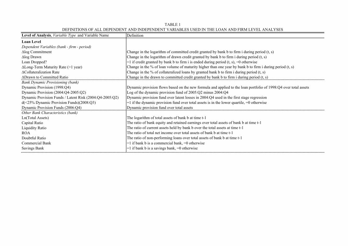

Level of Analysis Variable Type and Variable Name Unit MeanStandard
Deviation Minimum Median MaximumLoan LevelDependent Variables (bank - firm 2000Q1-2001Q2)ǻlog Commitment - -002 077 -234 -003 247ǻlog Drawn - -001 081 -230 -003 251Loan Dropped 01 025 043 0 0 1ǻLong-Term Maturity Rate (gt1 year) - 000 032 -100 000 100ǻCollateralization Rate - 000 018 -100 000 100ǻDrawn to Committed Ratio - -023 032 -100 -020 100Bank Dynamic Provisioning (bank 1998Q4)Dynamic Provision 026 010 000 022 086Other Bank Characteristics (bank)Ln(Total Assets) Ln(000 Euros) 1703 172 908 1712 1956Capital Ratio 601 208 000 529 5386Liquidity Ratio 2840 878 003 2917 9347ROA 133 074 -1608 108 469Doubtful Ratio 115 048 000 103 329Commercial Bank 01 060 049 0 1 1Savings Bank 01 035 048 0 0 1Bank-Firm Relationship Characteristic (bank - firm)Ln(1+Number of months with the bank) Ln(1+Months) 352 126 000 376 521Firm Characteristics (firm)Ln(Total Assets) Ln(000 Euros) 737 158 220 716 1712Capital Ratio 2332 1703 000 1967 9796Liquidity Ratio 566 777 000 294 10000ROA 732 732 -2550 628 5536Bad Credit History 01 016 037 0 0 1Ln(Age+1) Ln(1+Years) 230 079 000 240 487Tangible Assets 2491 2172 000 1922 10000Loan Characteristics (bank - firm)Maturity lt1 year 01 057 044 0 1 1Maturity 1-5 years 01 027 039 0 0 1Collateralized Loan 01 015 033 0 0 1Ln(Loan Amount) Ln(000 Euros) 400 195 000 420 1346
Firm LevelDependent Variables (firm ) -ǻlog Commitment (2000Q1-2001Q2) - -005 052 -237 -006 198ǻlog Drawn (2000Q1-2001Q2) - -004 057 -240 -006 220ǻlog Total Assets (1999Q4-2001Q4) - 043 036 -061 039 182ǻlog Employees (1999Q4-2001Q4) - 010 042 -139 005 170Firm Death (2001) 01 003 017 0 0 1
Loan Application LevelDependent Variable (bank-firm 2002M2-2002M12)Loan Application Is Accepted and Granted 01 038 049 0 0 1
TABLE 2SUMMARY STATISTICS FOR DEPENDENT AND INDEPENDENT VARIABLES USED IN THE LOAN AND FIRM LEVEL ANALYSIS
OF THE INTRODUCTION OF DYNAMIC PROVISIONING IN 2000Q3
NOTE -- Table 1 contains all variable definitions The number observations at the loan level 666698 at the firm level 76593 at the loanapplication level 15253
Model (1) (2) (3) (4) (5) (6) (7) (8) (9) (10) (11)Level
Dep
ende
nt V
aria
ble
ǻlog
Com
mitm
ent
(200
0Q
1-20
01Q
2)
ǻlog
Com
mitm
ent
(200
0Q
1-20
01Q
2)
ǻlog
Com
mitm
ent
(200
0Q
1-20
01Q
2)
ǻlog
Com
mitm
ent
(200
0Q
1-20
01Q
2)
ǻlog
Com
mitm
ent
(200
0Q
1-20
01Q
2)
ǻlog
Com
mitm
ent
(200
0Q
1-20
01Q
2)
ǻlog
Com
mitm
ent
(200
0Q
1-20
01Q
2)
2-St
age
Leas
t Squ
ares
ǻl
og C
omm
itmen
t
(200
0Q
1-20
01Q
2)
ǻlog
Dra
wn
(200
0Q
1-20
01Q
2)
Loan
Dro
pped
Loan
Dro
pped
Dynamic Provision (1998Q4)b -0336 -0366 -0366 -0357 -0259 -0389 -0397 -0575 -0451 0115 0104( 164) ( 186) ( 168) ( 123) ( 12) ( 147) ( 106) (169) ( 108) ( 117) ( 123)
Other Bank Characteristics Yes Yes Yes Yes Yes Yes Yes Yes Yes Yes YesBank-Firm Relationship Characteristic Yes Yes Yes Yes Yes Yes Yes Yes Yes Yes YesLoan Characteristics No No No No Yes No No No No No YesProvince and Industry Fixed effects Yes Yes Yes -- -- -- -- -- -- -- --Firm Fixed Effects No No No Yes Yes Yes -- -- -- Yes YesFirm Bank Type Fixed Effects No No No No No No Yes Yes Yes No NoSample with Multiple Bank-Firm Relationships Only No No Yes Yes Yes Yes Yes Yes Yes Yes YesSample with Firm Characteristics Only No Yes No No No Yes No No No No NoCluster Bank Bank Bank Bank Bank Bank Bank Bank Bank Bank BankNumber of Observations 666698 313234 416611 416611 416611 237905 416611 416611 366364 571007 571007
Model (12) (13) (14) (15) (16) (17) (18) (19) (20)
Level
Dep
ende
nt V
aria
ble
ǻLon
g-Te
rm M
atur
ity R
ate
(gt1
year
)
(200
0Q
1-20
01Q
2)
ǻCol
late
raliz
atio
n R
ate
(200
0Q
1-20
01Q
2)
ǻDra
wn
to C
omm
itted
Rat
io
(200
0Q
1-20
01Q
2)
ǻlog
Com
mitm
ent
(200
0Q
1-20
01Q
2)
ǻlog
Com
mitm
ent
(200
0Q
1-20
01Q
2)
ǻlog
Tot
al A
sset
s
(199
9Q
4-20
01Q
4)
ǻlog
Em
ploy
ees
(199
9Q
4-20
01Q
4)
Firm
Dea
th
(in
2001
)
Loan
App
licat
ion
Is A
ccep
ted
and
Gra
nted
(200
2M
2-20
02M
12)
Dynamic Provision (1998Q4)b -0163 0082 -0030 0010 0014 -0001 -0099 0000 0168( 049) ( 03) ( 04) ( 109) ( 103) ( 002) ( 067) ( 013) ( 153)
Other Bank Characteristics Yes Yes Yes Yes Yes Yes Yes Yes YesBank-Firm Relationship Characteristic Yes Yes Yes Yes Yes Yes Yes Yes YesFirm Characteristics -- -- -- Yes Yes Yes Yes Yes NoLoan Characteristics Yes Yes Yes No Yes No No No NoProvince and Industry Fixed effects -- -- -- Yes Yes Yes Yes Yes --Firm Fixed Effects Yes Yes Yes gt lt gt lt gt lt gt lt gt lt Firm-TimeSample with Multiple Bank-Firm Relationships Only Yes Yes Yes Yes Yes Yes Yes Yes NoSample with Firm Characteristics Only No No No Yes Yes Yes Yes Yes NoCluster Bank Bank Bank Main Bank Main Bank Main Bank Main Bank Main Bank BankNumber of Observations 416611 416611 416611 76593 76593 59449 41146 92576 15253
LOAN AND FIRM LEVEL ANALYSIS OF THE EFFECTS OF THE INTRODUCTION OF DYNAMIC PROVISIONING IN 2000Q3
FirmLoan
Application
Loan
TABLE 3
NOTE -- Model 6 corresponds to Equation 1 the adjacent text explains Models 1 to 14 In Model 8 in the first stage we regress Dynamic Provision Funds (2000Q1 - 2001Q2) on Dynamic Provision (1998Q4) The estimated coefficient equals0691 (0188) In the second stage the instrumented Dynamic Provision Funds (2000Q1 - 2001Q2) replaces Dynamic Provision (1998Q4) Model 15 corresponds to Equation 2 the adjacent text explains Models 15 to 19 Model 20 correspondsto Equation 3 Table 2 contains the list of variables for each set of characteristics and Table 1 the definition of all variables The Ln(Loan Amount) included in the Loan Characteristics is averaged from 1998Q4 to 1999Q4 Coefficients are listed in thefirst row robust standard errors that are corrected for clustering at the indicated level are reported in the row below in parentheses and the corresponding significance levels are in the adjacent column Yes indicates that the set of characteristics orfixed effects is included No indicates that the set of characteristics or fixed effects is not included gt lt indicates that the set of fixed effects cannot be included (because the regression is cross-sectional at the level of the fixed effects) -- indicatesthat the indicated set of characteristics or fixed effects are comprised in the wider included set of fixed effects Significant at 1 significant at 5 significant at 10
Loan
Model ( 1) ( 2) ( 3) ( 4) ( 5) ( 6)Dynamic Provision (1998Q4)b [=DPb] -4635 -0546 -0594 -0152 -4932
( 623) ( 316) ( 15) ( 267) ( 787)DPb Ln(Total Assetsb) 0273 0315
( 042) ( 057)DPb Capital Ratiob 0041 0041
( 037) ( 035)DPb ROAb 0202 -0168
( 088) ( 107)DPb Doubtful Ratiob -0192 -0207
( 148) ( 144)DPb Ln(Total Assetsf) 0027 0043 0043
( 025) ( 025) ( 025)DPb Capital Ratiof -0005 -0006 -0007
( 002) ( 002) ( 002)DPb ROAf -0006 -0003 -0002
( 003) ( 003) ( 003)DPb Bad Credit Historyf 0039 0000 -0003
( 063) ( 066) ( 065)DPb Ln(1+Number of months with the bank)bf -0025 -0046
( 046) ( 042)Other Bank Characteristics Yes Yes Yes Yes Yes YesBank-Firm Relationship Characteristic Yes Yes Yes Yes Yes YesFirm Fixed effects Yes Yes Yes Yes Yes YesBank Fixed effects No No No No No YesSample with Multiple Bank-Firm Relationships Only Yes Yes Yes Yes Yes YesSample with Firm Characteristics Only Yes Yes Yes Yes Yes YesCluster Bank Firm Bank Firm Bank Firm Bank Firm Bank Firm Bank FirmNumber of Observations 237905 237905 237905 237905 237905 237905NOTE -- The dependent variable is the ǻlog Commitment (2000Q1-2001Q2) Table 2 contains the list of variables for each set of characteristics and Table 1
contains all variable definitions Coefficients are listed in the first row robust standard errors that are corrected for clustering at the indicated level are reported in therow below in parentheses and the corresponding significance levels are in the adjacent column Yes indicates that the set of characteristics or fixed effects isincluded Significant at 1 significant at 5 significant at 10
ANALYSIS OF THE CHANGES IN COMMITTED LENDING AT THE INTRODUCTION OF DYNAMIC PROVISIONING IN 2000Q3 ACROSS BANKS AND FIRMS
TABLE 4
Level of Analysis Variable Type and Variable Name Unit MeanStandard
Deviation Minimum Median MaximumLoan LevelDependent Variables (bank - firm 2008Q1-2009Q4)ǻlog Commitment - -025 075 -281 -014 207ǻlog Drawn - -022 085 -294 -015 262Loan Dropped 01 030 046 0 0 1ǻLong-Term Maturity Rate (gt1 year) - 008 039 -100 000 100ǻCollateralization Rate - 005 023 -100 000 100ǻDrawn to Committed Ratio - -026 031 -100 -023 100Bank Dynamic Provisioning (bank)d(lt25 Dynamic Provision Funds)(2008Q3) 01 042 049 0 0 1Dynamic Provision Funds (2007Q4) 117 023 006 114 257Other Bank Characteristics (bank)Ln(Total Assets) Ln(000 Euros) 1786 150 910 1817 1973Capital Ratio 557 193 172 530 7329Liquidity Ratio 1237 626 036 1064 9725ROA 110 056 -023 097 344Doubtful Ratio 115 067 000 093 1205Commercial Bank 01 051 050 0 1 1Savings Bank 01 043 050 0 0 1Bank-Firm Relationship Characteristic (bank - firm)Ln(1+Number of months with the bank) Ln(1+Months) 379 117 000 393 563Firm Characteristics (firm)Ln(Total Assets) Ln(000 Euros) 795 168 220 774 1824Capital Ratio 2355 1787 000 1934 9947Liquidity Ratio 496 781 000 212 10000ROA 566 712 -3258 485 5588Bad Credit History 01 014 034 0 0 1Ln(Age+1) Ln(1+Years) 252 070 000 256 493Tangible Assets 2561 2372 000 1868 10000Loan Characteristics (bank - firm)Maturity lt1 year 01 050 045 0 0 1Maturity 1-5 years 01 025 038 0 0 1Collateralized loans 01 024 040 0 0 1Ln(Loan amount) Ln(000 Euros) 510 152 022 495 1390
Firm LevelDependent Variables (firm)ǻlog Commitment (2008Q1 to 2009Q4) - -027 053 -280 -019 164ǻlog Drawn (2008Q1 to 2009Q4) - -023 058 -295 -017 222ǻLog Total Assets (2007Q4 to 2009Q4) - -002 029 -091 -003 098ǻLog Employees (2007Q4 to 2009Q4) - -011 047 -177 -005 139Firm Death (in 2009) 01 006 023 000 000 100
Loan Application LevelDependent Variable (bank-firm)Loan Application Is Accepted and Granted (2008M10-2010M12) 01 028 045 0 0 1
TABLE 5
SUMMARY STATISTICS FOR DEPENDENT AND INDEPENDENT VARIABLES USED IN THE LOAN AND FIRM LEVEL ANALYSIS OF THE REMOVAL OF THE FLOOR VALUE OF DYNAMIC PROVISIONING IN 2008Q4 AND GOING INTO THE CRISIS WITH A
CERTAIN LEVEL OF DYNAMIC PROVISION FUNDS BUILT UP IN 2007Q4
NOTE ͲͲ Table 1 contains all variable definitions The number observations at the loan level 1101806 at the firm level 118616 at the loan applicationlevel61139
Model (1) (2) (3) (4) (5) (6) (7) (8) (9) (10) (11)Level
Dep
ende
nt V
aria
ble
ǻlog
Com
mitm
ent
(200
8Q
1-20
09Q
4)
ǻlog
Com
mitm
ent
(200
8Q
1-20
09Q
4)
ǻlog
Com
mitm
ent
(200
8Q
1-20
09Q
4)
ǻlog
Com
mitm
ent
(200
8Q
1-20
09Q
4)
ǻlog
Com
mitm
ent
(200
8Q
1-20
09Q
4)
ǻlog
Com
mitm
ent
(200
8Q
1-20
09Q
4)
ǻlog
Com
mitm
ent
(200
8Q
1-20
09Q
4)
2-St
age
Leas
t Sq
uare
s ǻl
og
Com
mitm
ent
(200
8Q
1-20
09Q
4)
ǻlog
Dra
wn
(200
8Q
1-20
09Q
4)
Loan
Dro
pped
Loan
Dro
pped
d(lt25 Dynamic Provision Funds)(2008Q3)b 0070 0077 0086 0094 0098 0096 0100 0086 0100 -0046 -0038
( 023) ( 028) ( 028) ( 026) ( 024) ( 03) ( 031) ( 029) ( 029) ( 014) ( 014)Dynamic Provision Funds (2007Q4)b 0096 0144 0130 0160 0172 0201 0191 0450 0198 -0054 -0057
( 05) ( 066) ( 066) ( 059) ( 058) ( 069) ( 07) ( 101) ( 061) ( 03) ( 03)Other Bank Characteristics Yes Yes Yes Yes Yes Yes Yes Yes Yes Yes YesBank-Firm Relationship Characteristic Yes Yes Yes Yes Yes Yes Yes Yes Yes Yes YesLoan Characteristics No No No No Yes No No No No No YesProvince and Industry Fixed effects Yes Yes Yes -- -- -- -- -- -- -- --Firm Fixed effects No No No Yes Yes Yes -- -- -- Yes YesFirm Bank Type Fixed Effects No No No No No No Yes Yes Yes No NoSample with Multiple Bank-Firm Relationships Only No No Yes Yes Yes Yes Yes Yes Yes Yes YesSample with Firm Characteristics Only No Yes No No No Yes No No No No NoCluster Bank Bank Bank Bank Bank Bank Bank Bank Bank Bank BankNumber of Observations 1101806 510582 687408 687408 687408 379821 687408 687408 622824 1018699 1018699
Model (12) (13) (14) (15) (16) (17) (18) (19) (20)
Level
Dep
ende
nt V
aria
ble
ǻLon
g-Te
rm M
atur
ity R
ate
(gt1
year
)
(200
8Q
1-20
09Q
4)
ǻCol
late
raliz
atio
n R
ate
(200
8Q
1-20
09Q
4)
ǻDra
wn
to C
omm
itted
Rat
io
(200
8Q
1-20
09Q
4)
ǻlog
Com
mitm
ent
(200
8Q
1-20
09Q
4)
ǻlog
Com
mitm
ent
(200
8Q
1-20
09Q
4)
ǻlog
Tot
al A
sset
s
(200
7Q
4-20
09Q
4)
ǻlog
Em
ploy
ees
(200
7Q
4-20
09Q
4)
Firm
Dea
th
(in
2009
)
Loan
App
licat
ion
Is A
ccep
ted
and
Gra
nted
(200
8M
10-2
010
M12
)
d(lt25 Dynamic Provision Funds)(2008Q3)b -0074 0012 0028 0058 0051 0007 -0005 0002 -0056 ( 021) ( 004) ( 007) ( 015) ( 014) ( 004) ( 006) ( 001) ( 015)
Dynamic Provision Funds (2007Q4)b -0175 0031 0013 0105 0111 0025 0027 -0008 0094 ( 047) ( 01) ( 015) ( 036) ( 035) ( 011) ( 014) ( 004) ( 042)
Other Bank Characteristics Yes Yes Yes Yes Yes Yes Yes Yes YesBank-Firm Relationship Characteristic Yes Yes Yes Yes Yes Yes Yes Yes YesFirm Characteristics -- -- -- Yes Yes Yes Yes Yes NoLoan Characteristics Yes Yes Yes No Yes No No No NoProvince and Industry Fixed effects -- -- -- Yes Yes Yes Yes Yes --Firm Fixed Effects Yes Yes Yes gt lt gt lt gt lt gt lt gt lt Firm-TimeSample with Multiple Bank-Firm Relationships Only Yes Yes Yes Yes Yes Yes Yes Yes NoSample with Firm Characteristics Only No No No Yes Yes Yes Yes Yes NoCluster Bank Bank Bank Main Bank Main Bank Main Bank Main Bank Main Bank BankNumber of Observations 687408 687408 687408 118616 118616 79183 71532 149304 61139
LOANANDFIRMLEVELANALYSISOFTHEEFFECTSOFTHEFLOORREMOVALOFDYNAMICPROVISIONINGIN2008Q4ANDOFGOINGINTOTHECRISISWITHACERTAINLEVELOFDYNAMICPROVISIONFUNDSBUILTUPIN2007Q4TABLE6
NOTE ͲͲ Model 6 corresponds to Equation 1 the adjacent text explains Models 1 to 14 In Model 8 in the first stage we regress Dynamic Provision Funds (2007Q4) on the simulated Dynamic Provision Funds (2007Q4) fixing the bank loan portfolio in 2000Q3 Theestimated coefficient equals 0772 (0133) In the second stage the inͲthisͲway instrumented Dynamic Provision Funds (2007Q4) replaces the actual Dynamic Provision Funds (2007Q4) Model 15 corresponds to Equation 2 the adjacent text explains Models 15 to19 Model 20 corresponds to Equation 3 Table 5 contains the list of variables for each set of characteristics and Table 1 the definition of all variables The Ln(Loan Amount) included in the Loan Characteristics is averaged from 2005Q4 to 2007Q1 Coefficients are listedin the first row robust standard errors that are corrected for clustering at the indicated level are reported in the row below in parentheses and the corresponding significance levels are in the adjacent column Yes indicates that the set of characteristics or fixed effectsis included No indicates that the set of characteristics or fixed effects is not included gt lt indicates that the set of fixed effects cannot be included (because the regression is crossͲsectional at the level of the fixed effects) ͲͲ indicates that the indicated set ofcharacteristicsorfixedeffectsarecomprisedinthewiderincludedsetoffixedeffectsSignificantat1significantat5significantat10
Loan
Loan FirmLoan
Application
Model ( 1) ( 2) ( 3) ( 4) ( 5) ( 6)d(lt25 Dynamic Provision Funds)(2008Q3)b [=DPb] -0392 0098 0148 0226 0380
( 229) ( 077) ( 15) ( 045) ( 226)DPb Ln(Total Assetsb) 0032 -0002
( 013) ( 012)DPb Capital Ratiob 0004 0009
( 013) ( 013)DPb ROAb -0050 -0074
( 048) ( 053)DPb Doubtful Ratiob -0125 -0134
( 029) ( 031)DPb Ln(Total Assetsf) -0011 -0011 -0006
( 004) ( 004) ( 003)DPb Capital Ratiof -0001 -0001 -0001
( 0004) ( 0003) ( 0003)DPb ROAf 0000 0000 0001
( 001) ( 001) ( 001)DPb Bad Credit Historyf -0003 0002 0004
( 01) ( 009) ( 009)DPb Ln(1+Number of months with the bank)bf 0005 0005
( 007) ( 006)Dynamic Provision Funds (2007Q4)b [=DPFb] -0285 0147 0256 0399 0166
( 275) ( 125) ( 15) ( 08) ( 414)DPFb Ln(Total Assetsb) 0023 0007
( 016) ( 018)DPFb Capital Ratiob 0009 0004
( 017) ( 016)DPFb ROAb -0026 -0024
( 136) ( 139)DPFb Doubtful Ratiob -0148 -0125
( 033) ( 043)DPFb Ln(Total Assetsf) 0006 0004 -0002
( 01) ( 009) ( 01)DPFb Capital Ratiof 0000 0000 0000
( 001) ( 001) ( 001)DPFb ROAf -0001 -0001 -0001
( 002) ( 001) ( 001)DPFb Bad Credit Historyf -0021 -0033 -0039
( 018) ( 02) ( 02)DFPb Ln(1+Number of months with the bank)bf 0023 0022
( 014) ( 012)Other Bank Characteristics Yes Yes Yes Yes Yes YesBank-Firm Relationship Characteristic Yes Yes Yes Yes Yes YesFirm Fixed effects Yes Yes Yes Yes Yes YesBank Fixed effects No No No No No YesSample with Multiple Bank-Firm Relationships Only Yes Yes Yes Yes Yes YesSample with Firm Characteristics Only Yes Yes Yes Yes Yes YesCluster Bank Firm Bank Firm Bank Firm Bank Firm Bank Firm Bank FirmNumber of Observations 379821 379821 379821 379821 379821 379821NOTE -- The dependent variable is the ǻlog Commitment (2008Q1-2009Q4) Table 5 contains the list of variables for each set of characteristics and Table 1
contains all variable definitions Coefficients are listed in the first row robust standard errors that are corrected for clustering at the indicated level are reported inthe row below in parentheses and the corresponding significance levels are in the adjacent column Yes indicates that the set of characteristics or fixed effects isincluded Significant at 1 significant at 5 significant at 10
ANALYSIS OF THE CHANGES IN COMMITTED LENDING FOLLOWING THE FLOOR REMOVAL OF DYNAMIC PROVISIONING IN 2008Q4 AND OF GOING INTO THE CRISIS WITH A CERTAIN LEVEL OF DYNAMIC PROVISION FUNDS BUILT UP IN 2007Q4 ACROSS BANKS AND FIRMS
TABLE 7
APPENDIX
- FOR ONLINE PUBLICATION -
CALCULATION OF DYNAMIC PROVISIONS
Dynamic provisions are formula based The total loan loss provisions for a period are the
sum of the Specific plus General Provisions The per-period (ie the flow of) General
Provisions are computed as
௧ݏݏݒݎݎܩ ൌ ௧ݏܮοߙ ൬ߚ െ ௧ݏݏݒݎ௧ݏܮ
൰ ௧ (A1)ݏܮ
where Loanst is the stock of loans at the end of period t and Loanst its variation from the end
of period t-1 to the end of period t (positive in a lending expansion negative in a credit
decline) D and E are parameters set by the Banco de Espantildea the Spanish banking regulator
D is an estimate of the percent latent loss in the loan portfolio while E is the average along the
cycle of specific provisions in relative terms Hence the second term is the key counter-
cyclical component
The above formula is in fact a simplification There are six risk buckets or homogeneous
groups of risk to take into account the different nature of the distinct segments of the credit
market each of them with a different D and E parameter These groups (in ascending order of
risk) are the following
i) Negligible risk Includes cash and public-sector exposures (both loans and
securities) as well as interbank exposures
ii) Low risk Made up of mortgages with a loan-to-value (LTV) ratio below 80 and
exposures to corporations with an A or higher rating
iii) Medium-low risk Composed of mortgages with an LTV ratio above 80 and other
collateralized loans not previously mentioned
iv) Medium risk Made up of other loans including unrated or below-A rated corporate
exposures and exposures to small and medium-sized firms
v) Medium-high risk Consumer durables financing and finally
vi) High risk Credit card exposures and overdrafts
The values for D are (moving from lower to higher risk levels) 0 06 15 18 2 and 25
percent and those for E 0 011 044 065 11 and 164 percent These are the parameter
values as they were modified in 2005Q1 (our second policy experiment) after their
introduction in 2000Q3 (our first policy experiment)
The final formula to be applied by each bank is therefore
௧ݏݏݒݎݎܩ
ൌߙοݏܮ௧
ୀଵ൬ߚ െ
௧ݏݏݒݎ௧ݏܮ
൰ ௧ݏܮ
ୀଵ
(A2)
௧ݏݏݒݎݎܩ
ൌߙοݏܮ௧
ୀଵ ൭ߚݏܮ௧
ୀଵെ ௧൱ݏݏݒݎ
(A3)
Moreover there is a ceiling for the fund of general loan loss provisions fixed at 125
percent of the product of parameter Į and the total volume of credit exposures Therefore the
fund of general provisions should be below 125 percent of the latent loss of the loan portfolio
The objective of this ceiling is to avoid an excess of provisioning which might occur in a
long expansionary phase as specific provisions remain below the ȕ component whereas the Į
component contributes positively to the accumulation of provisions in the fund The ceiling is
intended to avoid a provision fund that keeps growing indefinitely producing unnecessarily
too high coverage ratios of non-performing loans
There was also a minimum floor value for the fund of general provisions at 33 percent of
the latent loss This minimum was lowered at the end of 2008 to 10 percent in order to allow
for more usage of the general provisions previously built in the expansionary period (our third
policy experiment)
TAX TREATEMENT OF DYNAMIC PROVISIONS
Regarding tax treatment general provisions are tax-deductible up to 1 percent of the
increase in gross loans as long as they are not mortgages Non-deductible amounts (ie those
above that threshold) are accounted for as deferred tax assets because they will become
specific provisions in the future and therefore deductible when the impairment is assigned to
an individual loan Before 2005 the countercyclical part of the loan loss provisions was not
tax-deductible
FIGUREA1ESTIMATESOFTIMEͲVARYINGCOEFFICIENTONTHEINDEPENDENTVARIABLEDYNAMICPROVISIONFORCOMMITMENTLENDING
NOTE ͲͲ Solid lines represent the coefficients of Dynamic Provision in Models 8 and 17 in Table A2 that are estimated with rolling time windows Dashed lines represent the two standard error confidence band drawn around the coefficient estimates Black lines are at theloanlevelbluelinesareatthefirmlevelTable1containsallvariabledefinitions
Ͳ04
Ͳ03
Ͳ02
Ͳ01
0
01
02
03
04
0520
05Q1
2005Q1
2005Q2
2005Q3
2005Q4
2006Q1
2006Q2
2006Q3
2006Q4
2007Q1
2007Q2
2007Q3
2007Q4
ȴLogCommitment
LoanLevel FirmLevel
Level of Analysis Variable Type and Variable Name Unit MeanStandard
Deviation Minimum Median MaximumLoan LevelDependent Variables (bank - firm 2004Q4-2006Q2)ǻlog Commitment - 001 093 -277 -006 305ǻlog Drawn - 001 080 -252 000 268Loan Dropped 01 026 044 0 0 1ǻLong-Term Maturity Rate (gt1 year) - 000 032 -100 000 100ǻCollateralization Rate - 001 019 -100 000 100ǻDrawn to Committed Ratio - -025 031 -100 -022 100Bank Dynamic Provisioning (bank 2004Q4 to 2005Q2)Dynamic Provision 005 014 -018 000 037Dynamic Provision Funds Latent Risk - 133 018 026 138 205Other Bank Characteristics (bank)Ln(Total Assets) Ln(000 Euros) 1735 155 897 1763 1929Capital Ratio 631 309 178 559 5337Liquidity Ratio 1818 722 003 1835 8913ROA 094 050 -323 089 563Doubtful Ratio 066 040 000 055 5356Commercial Bank 01 054 050 0 1 1Savings Bank 01 040 049 0 0 1Bank-Firm Relationship Characteristic (bank - firm)Ln(1+Number of months with the bank) Ln(1+Months) 376 117 000 395 548Firm Characteristics (firm)Ln(Total Assets) Ln(000 Euros) 749 165 161 730 1771Capital Ratio 2460 1797 001 2074 9957Liquidity Ratio 597 871 000 286 10000ROA 613 776 -3548 517 6316Bad Credit History 01 013 034 0 0 1Ln(Age+1) Ln(1+Years) 235 078 000 240 490Tangible Assets 2613 2332 000 1966 10000Loan Characteristics (bank - firm)Maturity lt1 year 01 055 044 0 1 1Maturity 1-5 years 01 024 037 0 0 1Collateralized Loan 01 019 037 0 0 1Ln(Loan Amount) Ln(000 Euros) 460 174 000 460 1358
Firm LevelDependent Variables (firm ) -ǻlog Commitment (2004Q4-2006Q2) - -001 058 -259 -003 236ǻlog Drawn (2004Q4-2006Q2) - -001 064 -278 -004 270ǻlog Total Assets (2004Q4-2006Q4) - 017 038 -092 011 165ǻlog Employees (2004Q4-2006Q4) - 007 041 -139 000 161Firm Death (2006) 01 002 015 0 0 1
Loan Application LevelDependent Variable (bank-firm 2005M7-2006M12)Loan Application Is Accepted and Granted 01 040 049 0 0 1
TABLE A1SUMMARY STATISTICS FOR DEPENDENT AND INDEPENDENT VARIABLES USED IN THE LOAN AND FIRM LEVEL ANALYSIS OF
THE MODIFICATION OF DYNAMIC PROVISIONING IN 2005Q1
NOTE -- Table 1 contains all variable definitions The number observations at the loan level 884859 at the firm level 107087 at the loanapplication level 71050
Model (1) (2) (3) (4) (5) (6) (7) (8) (9) (10)Level
Dep
ende
nt V
aria
ble
ǻlog
Com
mitm
ent
(200
4Q
4-20
06Q
2)
ǻlog
Com
mitm
ent
(200
4Q
4-20
06Q
2)
ǻlog
Com
mitm
ent
(200
4Q
4-20
06Q
2)
ǻlog
Com
mitm
ent
(200
4Q
4-20
06Q
2)
ǻlog
Com
mitm
ent
(200
4Q
4-20
06Q
2)
ǻlog
Com
mitm
ent
(200
4Q
4-20
06Q
2)
ǻlog
Com
mitm
ent
(200
4Q
4-20
06Q
2)
ǻlog
Dra
wn
(200
0Q
1-20
01Q
2)
Loan
Dro
pped
Loan
Dro
pped
Dynamic Provision(2004Q4-2005Q2)b -0111 -0120 -0124 -0108 -0040 -0115 -0045 -0100 0033 0046( 047) ( 054) ( 056) ( 048) ( 049) ( 048) ( 053) ( 0563) ( 037) ( 037)
Other Bank Characteristics Yes Yes Yes Yes Yes Yes Yes Yes Yes YesBank-Firm Relationship Characteristic Yes Yes Yes Yes Yes Yes Yes Yes Yes YesLoan Characteristics No No No No Yes No No No No YesProvince and Industry Fixed effects Yes Yes Yes -- -- -- -- -- -- --Firm Fixed Effects No No No Yes Yes Yes -- -- Yes YesFirm Bank Type Fixed Effects No No No No No No Yes Yes No NoSample with Multiple Bank-Firm Relationships Only No No Yes Yes Yes Yes Yes Yes YesSample with Firm Characteristics Only No Yes No No No Yes No No No NoCluster Bank Bank Bank Bank Bank Bank Bank Bank Bank BankNumber of Observations 884859 460885 543499 543499 543499 334631 543499 480359 750735 750735
Model (11) (12) (13) (14) (15) (16) (17) (18) (19)
Level
Dep
ende
nt V
aria
ble
ǻLon
g-Te
rm M
atur
ity R
ate
(gt1
year
)
(200
4Q
4-20
06Q
2)
ǻCol
late
raliz
atio
n R
ate
(200
4Q
4-20
06Q
2)
ǻDra
wn
to C
omm
itted
Rat
io
(200
4Q
4-20
06Q
2)
ǻlog
Com
mitm
ent
(200
4Q
4-20
06Q
2)
ǻlog
Com
mitm
ent
(200
4Q
4-20
06Q
2)
ǻlog
Tot
al A
sset
s
(200
4Q
4-20
06Q
4)
ǻlog
Em
ploy
ees
(200
4Q
4-20
06Q
4)
Firm
Dea
th
(in
2006
)
Loan
App
licat
ion
Is A
ccep
ted
and
Gra
nted
(200
5M
7-20
06M
12)
Dynamic Provision(2004Q4-2005Q2)b -0065 0022 0009 -0074 -0039 0003 0014 -0004 -0003( 064) ( 011) ( 057) ( 038) ( 033) ( 02) ( 022) ( 006) ( 046)
Other Bank Characteristics Yes Yes Yes Yes Yes Yes Yes Yes YesBank-Firm Relationship Characteristic Yes Yes Yes Yes Yes Yes Yes Yes YesFirm Characteristics -- -- -- Yes Yes Yes Yes Yes NoLoan Characteristics Yes Yes Yes No Yes No No No NoProvince and Industry Fixed effects -- -- -- Yes Yes Yes Yes Yes --Firm Fixed Effects Yes Yes Yes gt lt gt lt gt lt gt lt gt lt Firm-TimeSample with Multiple Bank-Firm Relationships Only Yes Yes Yes Yes Yes Yes Yes Yes NoSample with Firm Characteristics Only No No No Yes Yes Yes Yes Yes NoCluster Bank Bank Bank Main Bank Main Bank Main Bank Main Bank Main Bank BankNumber of Observations 543499 543499 327233 107087 107087 79877 68737 132634 71050
LOAN AND FIRM LEVEL ANALYSIS OF THE EFFECTS OF THE MODIFICATION OF DYNAMIC PROVISIONING IN 2005Q1
Loan
Loan
FirmLoan
Application
TABLE A2
NOTE -- Model 6 corresponds to Equation 1 the adjacent text explains Models 1 to 13 Model 14 corresponds to Equation 2 the adjacent text explains Models 14 to 18 Model 19 corresponds to Equation 3 The instrumentation ofDynamic Provision is explained in Equation 3 and adjacent text Table A1 contains the list of variables for each set of characteristics and Table 1 the definition of all variables The Ln(Loan Amount) included in the LoanCharacteristics is averaged from 2004Q4 to 2005Q4 Coefficients are listed in the first row robust standard errors that are corrected for clustering at the indicated level are reported in the row below in parentheses and thecorresponding significance levels are in the adjacent column Yes indicates that the set of characteristics or fixed effects is included No indicates that the set of characteristics or fixed effects is not included gt lt indicates thatthe set of fixed effects cannot be included (because the regression is cross-sectional at the level of the fixed effects) -- indicates that the indicated set of characteristics or fixed effects are comprised in the wider included set of fixedeffects Significant at 1 significant at 5 significant at 10
Model ( 1) ( 2) ( 3) ( 4) ( 5) ( 5)Dynamic Provision(2004Q4-2005Q2)b [=DPb] -1986 0133 -0135 0159 -4736
( 658) ( 323) ( 15) ( 716) ( 16505)DPb Ln(Total Assetsb) 0108 0249
( 039) ( 778)DPb Capital Ratiob -0039 -0037
( 051) ( 186)DPb ROAb 0035 -0172
( 1) ( 324)DPb Doubtful Ratiob -0394 0955
( 1063) ( 6099)DPb Ln(Total Assetsf) 0010 0018 0002
( 015) ( 068) ( 015)DPb Capital Ratiof -0001 -0001 -0001
( 002) ( 003) ( 002)DPb ROAf -0002 -0002 -0002
( 002) ( 002) ( 002)DPb Bad Credit Historyf -0028 -0024 -0024
( 05) ( 099) ( 036)DPb Ln(1+Number of months with the bank)bf 0024 0004
( 038) ( 013)Other Bank Characteristics Yes Yes Yes Yes Yes YesBank-Firm Relationship Characteristic Yes Yes Yes Yes Yes YesFirm Fixed effects Yes Yes Yes Yes Yes YesBank Fixed effects No No No No No YesSample with Multiple Bank-Firm Relationships Only Yes Yes Yes Yes Yes YesSample with Firm Characteristics Only Yes Yes Yes Yes Yes YesCluster Bank Firm Bank Firm Bank Firm Bank Firm Bank Firm Bank FirmNumber of Observations 334631 334631 334631 334631 334631 334631NOTE -- The dependent variable is the ǻlog Commitment (2004Q4-2006Q2) Table A1 contains the list of variables for each set of characteristics and Table 1
contains all variable definitions Coefficients are listed in the first row robust standard errors that are corrected for clustering at the indicated level are reported in therow below in parentheses and the corresponding significance levels are in the adjacent column Yes indicates that the set of characteristics or fixed effects isincluded Significant at 1 significant at 5 significant at 10
ANALYSIS OF THE CHANGES IN COMMITTED LENDING AT THE MODIFICATION OF DYNAMIC PROVISIONING IN 2005Q1 ACROSS BANKS AND FIRMS
TABLE A3
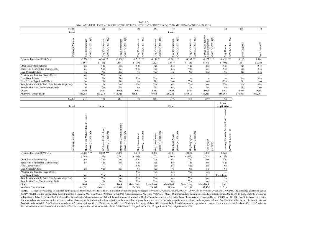
Model (1) (2) (3) (4) (5) (6) (7) (8) (9) (10) (11)Level
Dep
ende
nt V
aria
ble
ǻlog
Com
mitm
ent
(200
0Q
1-20
01Q
2)
ǻlog
Com
mitm
ent
(200
0Q
1-20
01Q
2)
ǻlog
Com
mitm
ent
(200
0Q
1-20
01Q
2)
ǻlog
Com
mitm
ent
(200
0Q
1-20
01Q
2)
ǻlog
Com
mitm
ent
(200
0Q
1-20
01Q
2)
ǻlog
Com
mitm
ent
(200
0Q
1-20
01Q
2)
ǻlog
Com
mitm
ent
(200
0Q
1-20
01Q
2)
2-St
age
Leas
t Squ
ares
ǻl
og C
omm
itmen
t
(200
0Q
1-20
01Q
2)
ǻlog
Dra
wn
(200
0Q
1-20
01Q
2)
Loan
Dro
pped
Loan
Dro
pped
Dynamic Provision (1998Q4)b -0336 -0366 -0366 -0357 -0259 -0389 -0397 -0575 -0451 0115 0104( 164) ( 186) ( 168) ( 123) ( 12) ( 147) ( 106) (169) ( 108) ( 117) ( 123)
Other Bank Characteristics Yes Yes Yes Yes Yes Yes Yes Yes Yes Yes YesBank-Firm Relationship Characteristic Yes Yes Yes Yes Yes Yes Yes Yes Yes Yes YesLoan Characteristics No No No No Yes No No No No No YesProvince and Industry Fixed effects Yes Yes Yes -- -- -- -- -- -- -- --Firm Fixed Effects No No No Yes Yes Yes -- -- -- Yes YesFirm Bank Type Fixed Effects No No No No No No Yes Yes Yes No NoSample with Multiple Bank-Firm Relationships Only No No Yes Yes Yes Yes Yes Yes Yes Yes YesSample with Firm Characteristics Only No Yes No No No Yes No No No No NoCluster Bank Bank Bank Bank Bank Bank Bank Bank Bank Bank BankNumber of Observations 666698 313234 416611 416611 416611 237905 416611 416611 366364 571007 571007
Model (12) (13) (14) (15) (16) (17) (18) (19) (20)
Level
Dep
ende
nt V
aria
ble
ǻLon
g-Te
rm M
atur
ity R
ate
(gt1
year
)
(200
0Q
1-20
01Q
2)
ǻCol
late
raliz
atio
n R
ate
(200
0Q
1-20
01Q
2)
ǻDra
wn
to C
omm
itted
Rat
io
(200
0Q
1-20
01Q
2)
ǻlog
Com
mitm
ent
(200
0Q
1-20
01Q
2)
ǻlog
Com
mitm
ent
(200
0Q
1-20
01Q
2)
ǻlog
Tot
al A
sset
s
(199
9Q
4-20
01Q
4)
ǻlog
Em
ploy
ees
(199
9Q
4-20
01Q
4)
Firm
Dea
th
(in
2001
)
Loan
App
licat
ion
Is A
ccep
ted
and
Gra
nted
(200
2M
2-20
02M
12)
Dynamic Provision (1998Q4)b -0163 0082 -0030 0010 0014 -0001 -0099 0000 0168( 049) ( 03) ( 04) ( 109) ( 103) ( 002) ( 067) ( 013) ( 153)
Other Bank Characteristics Yes Yes Yes Yes Yes Yes Yes Yes YesBank-Firm Relationship Characteristic Yes Yes Yes Yes Yes Yes Yes Yes YesFirm Characteristics -- -- -- Yes Yes Yes Yes Yes NoLoan Characteristics Yes Yes Yes No Yes No No No NoProvince and Industry Fixed effects -- -- -- Yes Yes Yes Yes Yes --Firm Fixed Effects Yes Yes Yes gt lt gt lt gt lt gt lt gt lt Firm-TimeSample with Multiple Bank-Firm Relationships Only Yes Yes Yes Yes Yes Yes Yes Yes NoSample with Firm Characteristics Only No No No Yes Yes Yes Yes Yes NoCluster Bank Bank Bank Main Bank Main Bank Main Bank Main Bank Main Bank BankNumber of Observations 416611 416611 416611 76593 76593 59449 41146 92576 15253
LOAN AND FIRM LEVEL ANALYSIS OF THE EFFECTS OF THE INTRODUCTION OF DYNAMIC PROVISIONING IN 2000Q3
FirmLoan
Application
Loan
TABLE 3
NOTE -- Model 6 corresponds to Equation 1 the adjacent text explains Models 1 to 14 In Model 8 in the first stage we regress Dynamic Provision Funds (2000Q1 - 2001Q2) on Dynamic Provision (1998Q4) The estimated coefficient equals0691 (0188) In the second stage the instrumented Dynamic Provision Funds (2000Q1 - 2001Q2) replaces Dynamic Provision (1998Q4) Model 15 corresponds to Equation 2 the adjacent text explains Models 15 to 19 Model 20 correspondsto Equation 3 Table 2 contains the list of variables for each set of characteristics and Table 1 the definition of all variables The Ln(Loan Amount) included in the Loan Characteristics is averaged from 1998Q4 to 1999Q4 Coefficients are listed in thefirst row robust standard errors that are corrected for clustering at the indicated level are reported in the row below in parentheses and the corresponding significance levels are in the adjacent column Yes indicates that the set of characteristics orfixed effects is included No indicates that the set of characteristics or fixed effects is not included gt lt indicates that the set of fixed effects cannot be included (because the regression is cross-sectional at the level of the fixed effects) -- indicatesthat the indicated set of characteristics or fixed effects are comprised in the wider included set of fixed effects Significant at 1 significant at 5 significant at 10
Loan
Model ( 1) ( 2) ( 3) ( 4) ( 5) ( 6)Dynamic Provision (1998Q4)b [=DPb] -4635 -0546 -0594 -0152 -4932
( 623) ( 316) ( 15) ( 267) ( 787)DPb Ln(Total Assetsb) 0273 0315
( 042) ( 057)DPb Capital Ratiob 0041 0041
( 037) ( 035)DPb ROAb 0202 -0168
( 088) ( 107)DPb Doubtful Ratiob -0192 -0207
( 148) ( 144)DPb Ln(Total Assetsf) 0027 0043 0043
( 025) ( 025) ( 025)DPb Capital Ratiof -0005 -0006 -0007
( 002) ( 002) ( 002)DPb ROAf -0006 -0003 -0002
( 003) ( 003) ( 003)DPb Bad Credit Historyf 0039 0000 -0003
( 063) ( 066) ( 065)DPb Ln(1+Number of months with the bank)bf -0025 -0046
( 046) ( 042)Other Bank Characteristics Yes Yes Yes Yes Yes YesBank-Firm Relationship Characteristic Yes Yes Yes Yes Yes YesFirm Fixed effects Yes Yes Yes Yes Yes YesBank Fixed effects No No No No No YesSample with Multiple Bank-Firm Relationships Only Yes Yes Yes Yes Yes YesSample with Firm Characteristics Only Yes Yes Yes Yes Yes YesCluster Bank Firm Bank Firm Bank Firm Bank Firm Bank Firm Bank FirmNumber of Observations 237905 237905 237905 237905 237905 237905NOTE -- The dependent variable is the ǻlog Commitment (2000Q1-2001Q2) Table 2 contains the list of variables for each set of characteristics and Table 1
contains all variable definitions Coefficients are listed in the first row robust standard errors that are corrected for clustering at the indicated level are reported in therow below in parentheses and the corresponding significance levels are in the adjacent column Yes indicates that the set of characteristics or fixed effects isincluded Significant at 1 significant at 5 significant at 10
ANALYSIS OF THE CHANGES IN COMMITTED LENDING AT THE INTRODUCTION OF DYNAMIC PROVISIONING IN 2000Q3 ACROSS BANKS AND FIRMS
TABLE 4
Level of Analysis Variable Type and Variable Name Unit MeanStandard
Deviation Minimum Median MaximumLoan LevelDependent Variables (bank - firm 2008Q1-2009Q4)ǻlog Commitment - -025 075 -281 -014 207ǻlog Drawn - -022 085 -294 -015 262Loan Dropped 01 030 046 0 0 1ǻLong-Term Maturity Rate (gt1 year) - 008 039 -100 000 100ǻCollateralization Rate - 005 023 -100 000 100ǻDrawn to Committed Ratio - -026 031 -100 -023 100Bank Dynamic Provisioning (bank)d(lt25 Dynamic Provision Funds)(2008Q3) 01 042 049 0 0 1Dynamic Provision Funds (2007Q4) 117 023 006 114 257Other Bank Characteristics (bank)Ln(Total Assets) Ln(000 Euros) 1786 150 910 1817 1973Capital Ratio 557 193 172 530 7329Liquidity Ratio 1237 626 036 1064 9725ROA 110 056 -023 097 344Doubtful Ratio 115 067 000 093 1205Commercial Bank 01 051 050 0 1 1Savings Bank 01 043 050 0 0 1Bank-Firm Relationship Characteristic (bank - firm)Ln(1+Number of months with the bank) Ln(1+Months) 379 117 000 393 563Firm Characteristics (firm)Ln(Total Assets) Ln(000 Euros) 795 168 220 774 1824Capital Ratio 2355 1787 000 1934 9947Liquidity Ratio 496 781 000 212 10000ROA 566 712 -3258 485 5588Bad Credit History 01 014 034 0 0 1Ln(Age+1) Ln(1+Years) 252 070 000 256 493Tangible Assets 2561 2372 000 1868 10000Loan Characteristics (bank - firm)Maturity lt1 year 01 050 045 0 0 1Maturity 1-5 years 01 025 038 0 0 1Collateralized loans 01 024 040 0 0 1Ln(Loan amount) Ln(000 Euros) 510 152 022 495 1390
Firm LevelDependent Variables (firm)ǻlog Commitment (2008Q1 to 2009Q4) - -027 053 -280 -019 164ǻlog Drawn (2008Q1 to 2009Q4) - -023 058 -295 -017 222ǻLog Total Assets (2007Q4 to 2009Q4) - -002 029 -091 -003 098ǻLog Employees (2007Q4 to 2009Q4) - -011 047 -177 -005 139Firm Death (in 2009) 01 006 023 000 000 100
Loan Application LevelDependent Variable (bank-firm)Loan Application Is Accepted and Granted (2008M10-2010M12) 01 028 045 0 0 1
TABLE 5
SUMMARY STATISTICS FOR DEPENDENT AND INDEPENDENT VARIABLES USED IN THE LOAN AND FIRM LEVEL ANALYSIS OF THE REMOVAL OF THE FLOOR VALUE OF DYNAMIC PROVISIONING IN 2008Q4 AND GOING INTO THE CRISIS WITH A
CERTAIN LEVEL OF DYNAMIC PROVISION FUNDS BUILT UP IN 2007Q4
NOTE ͲͲ Table 1 contains all variable definitions The number observations at the loan level 1101806 at the firm level 118616 at the loan applicationlevel61139
Model (1) (2) (3) (4) (5) (6) (7) (8) (9) (10) (11)Level
Dep
ende
nt V
aria
ble
ǻlog
Com
mitm
ent
(200
8Q
1-20
09Q
4)
ǻlog
Com
mitm
ent
(200
8Q
1-20
09Q
4)
ǻlog
Com
mitm
ent
(200
8Q
1-20
09Q
4)
ǻlog
Com
mitm
ent
(200
8Q
1-20
09Q
4)
ǻlog
Com
mitm
ent
(200
8Q
1-20
09Q
4)
ǻlog
Com
mitm
ent
(200
8Q
1-20
09Q
4)
ǻlog
Com
mitm
ent
(200
8Q
1-20
09Q
4)
2-St
age
Leas
t Sq
uare
s ǻl
og
Com
mitm
ent
(200
8Q
1-20
09Q
4)
ǻlog
Dra
wn
(200
8Q
1-20
09Q
4)
Loan
Dro
pped
Loan
Dro
pped
d(lt25 Dynamic Provision Funds)(2008Q3)b 0070 0077 0086 0094 0098 0096 0100 0086 0100 -0046 -0038
( 023) ( 028) ( 028) ( 026) ( 024) ( 03) ( 031) ( 029) ( 029) ( 014) ( 014)Dynamic Provision Funds (2007Q4)b 0096 0144 0130 0160 0172 0201 0191 0450 0198 -0054 -0057
( 05) ( 066) ( 066) ( 059) ( 058) ( 069) ( 07) ( 101) ( 061) ( 03) ( 03)Other Bank Characteristics Yes Yes Yes Yes Yes Yes Yes Yes Yes Yes YesBank-Firm Relationship Characteristic Yes Yes Yes Yes Yes Yes Yes Yes Yes Yes YesLoan Characteristics No No No No Yes No No No No No YesProvince and Industry Fixed effects Yes Yes Yes -- -- -- -- -- -- -- --Firm Fixed effects No No No Yes Yes Yes -- -- -- Yes YesFirm Bank Type Fixed Effects No No No No No No Yes Yes Yes No NoSample with Multiple Bank-Firm Relationships Only No No Yes Yes Yes Yes Yes Yes Yes Yes YesSample with Firm Characteristics Only No Yes No No No Yes No No No No NoCluster Bank Bank Bank Bank Bank Bank Bank Bank Bank Bank BankNumber of Observations 1101806 510582 687408 687408 687408 379821 687408 687408 622824 1018699 1018699
Model (12) (13) (14) (15) (16) (17) (18) (19) (20)
Level
Dep
ende
nt V
aria
ble
ǻLon
g-Te
rm M
atur
ity R
ate
(gt1
year
)
(200
8Q
1-20
09Q
4)
ǻCol
late
raliz
atio
n R
ate
(200
8Q
1-20
09Q
4)
ǻDra
wn
to C
omm
itted
Rat
io
(200
8Q
1-20
09Q
4)
ǻlog
Com
mitm
ent
(200
8Q
1-20
09Q
4)
ǻlog
Com
mitm
ent
(200
8Q
1-20
09Q
4)
ǻlog
Tot
al A
sset
s
(200
7Q
4-20
09Q
4)
ǻlog
Em
ploy
ees
(200
7Q
4-20
09Q
4)
Firm
Dea
th
(in
2009
)
Loan
App
licat
ion
Is A
ccep
ted
and
Gra
nted
(200
8M
10-2
010
M12
)
d(lt25 Dynamic Provision Funds)(2008Q3)b -0074 0012 0028 0058 0051 0007 -0005 0002 -0056 ( 021) ( 004) ( 007) ( 015) ( 014) ( 004) ( 006) ( 001) ( 015)
Dynamic Provision Funds (2007Q4)b -0175 0031 0013 0105 0111 0025 0027 -0008 0094 ( 047) ( 01) ( 015) ( 036) ( 035) ( 011) ( 014) ( 004) ( 042)
Other Bank Characteristics Yes Yes Yes Yes Yes Yes Yes Yes YesBank-Firm Relationship Characteristic Yes Yes Yes Yes Yes Yes Yes Yes YesFirm Characteristics -- -- -- Yes Yes Yes Yes Yes NoLoan Characteristics Yes Yes Yes No Yes No No No NoProvince and Industry Fixed effects -- -- -- Yes Yes Yes Yes Yes --Firm Fixed Effects Yes Yes Yes gt lt gt lt gt lt gt lt gt lt Firm-TimeSample with Multiple Bank-Firm Relationships Only Yes Yes Yes Yes Yes Yes Yes Yes NoSample with Firm Characteristics Only No No No Yes Yes Yes Yes Yes NoCluster Bank Bank Bank Main Bank Main Bank Main Bank Main Bank Main Bank BankNumber of Observations 687408 687408 687408 118616 118616 79183 71532 149304 61139
LOANANDFIRMLEVELANALYSISOFTHEEFFECTSOFTHEFLOORREMOVALOFDYNAMICPROVISIONINGIN2008Q4ANDOFGOINGINTOTHECRISISWITHACERTAINLEVELOFDYNAMICPROVISIONFUNDSBUILTUPIN2007Q4TABLE6
NOTE ͲͲ Model 6 corresponds to Equation 1 the adjacent text explains Models 1 to 14 In Model 8 in the first stage we regress Dynamic Provision Funds (2007Q4) on the simulated Dynamic Provision Funds (2007Q4) fixing the bank loan portfolio in 2000Q3 Theestimated coefficient equals 0772 (0133) In the second stage the inͲthisͲway instrumented Dynamic Provision Funds (2007Q4) replaces the actual Dynamic Provision Funds (2007Q4) Model 15 corresponds to Equation 2 the adjacent text explains Models 15 to19 Model 20 corresponds to Equation 3 Table 5 contains the list of variables for each set of characteristics and Table 1 the definition of all variables The Ln(Loan Amount) included in the Loan Characteristics is averaged from 2005Q4 to 2007Q1 Coefficients are listedin the first row robust standard errors that are corrected for clustering at the indicated level are reported in the row below in parentheses and the corresponding significance levels are in the adjacent column Yes indicates that the set of characteristics or fixed effectsis included No indicates that the set of characteristics or fixed effects is not included gt lt indicates that the set of fixed effects cannot be included (because the regression is crossͲsectional at the level of the fixed effects) ͲͲ indicates that the indicated set ofcharacteristicsorfixedeffectsarecomprisedinthewiderincludedsetoffixedeffectsSignificantat1significantat5significantat10
Loan
Loan FirmLoan
Application
Model ( 1) ( 2) ( 3) ( 4) ( 5) ( 6)d(lt25 Dynamic Provision Funds)(2008Q3)b [=DPb] -0392 0098 0148 0226 0380
( 229) ( 077) ( 15) ( 045) ( 226)DPb Ln(Total Assetsb) 0032 -0002
( 013) ( 012)DPb Capital Ratiob 0004 0009
( 013) ( 013)DPb ROAb -0050 -0074
( 048) ( 053)DPb Doubtful Ratiob -0125 -0134
( 029) ( 031)DPb Ln(Total Assetsf) -0011 -0011 -0006
( 004) ( 004) ( 003)DPb Capital Ratiof -0001 -0001 -0001
( 0004) ( 0003) ( 0003)DPb ROAf 0000 0000 0001
( 001) ( 001) ( 001)DPb Bad Credit Historyf -0003 0002 0004
( 01) ( 009) ( 009)DPb Ln(1+Number of months with the bank)bf 0005 0005
( 007) ( 006)Dynamic Provision Funds (2007Q4)b [=DPFb] -0285 0147 0256 0399 0166
( 275) ( 125) ( 15) ( 08) ( 414)DPFb Ln(Total Assetsb) 0023 0007
( 016) ( 018)DPFb Capital Ratiob 0009 0004
( 017) ( 016)DPFb ROAb -0026 -0024
( 136) ( 139)DPFb Doubtful Ratiob -0148 -0125
( 033) ( 043)DPFb Ln(Total Assetsf) 0006 0004 -0002
( 01) ( 009) ( 01)DPFb Capital Ratiof 0000 0000 0000
( 001) ( 001) ( 001)DPFb ROAf -0001 -0001 -0001
( 002) ( 001) ( 001)DPFb Bad Credit Historyf -0021 -0033 -0039
( 018) ( 02) ( 02)DFPb Ln(1+Number of months with the bank)bf 0023 0022
( 014) ( 012)Other Bank Characteristics Yes Yes Yes Yes Yes YesBank-Firm Relationship Characteristic Yes Yes Yes Yes Yes YesFirm Fixed effects Yes Yes Yes Yes Yes YesBank Fixed effects No No No No No YesSample with Multiple Bank-Firm Relationships Only Yes Yes Yes Yes Yes YesSample with Firm Characteristics Only Yes Yes Yes Yes Yes YesCluster Bank Firm Bank Firm Bank Firm Bank Firm Bank Firm Bank FirmNumber of Observations 379821 379821 379821 379821 379821 379821NOTE -- The dependent variable is the ǻlog Commitment (2008Q1-2009Q4) Table 5 contains the list of variables for each set of characteristics and Table 1
contains all variable definitions Coefficients are listed in the first row robust standard errors that are corrected for clustering at the indicated level are reported inthe row below in parentheses and the corresponding significance levels are in the adjacent column Yes indicates that the set of characteristics or fixed effects isincluded Significant at 1 significant at 5 significant at 10
ANALYSIS OF THE CHANGES IN COMMITTED LENDING FOLLOWING THE FLOOR REMOVAL OF DYNAMIC PROVISIONING IN 2008Q4 AND OF GOING INTO THE CRISIS WITH A CERTAIN LEVEL OF DYNAMIC PROVISION FUNDS BUILT UP IN 2007Q4 ACROSS BANKS AND FIRMS
TABLE 7
APPENDIX
- FOR ONLINE PUBLICATION -
CALCULATION OF DYNAMIC PROVISIONS
Dynamic provisions are formula based The total loan loss provisions for a period are the
sum of the Specific plus General Provisions The per-period (ie the flow of) General
Provisions are computed as
௧ݏݏݒݎݎܩ ൌ ௧ݏܮοߙ ൬ߚ െ ௧ݏݏݒݎ௧ݏܮ
൰ ௧ (A1)ݏܮ
where Loanst is the stock of loans at the end of period t and Loanst its variation from the end
of period t-1 to the end of period t (positive in a lending expansion negative in a credit
decline) D and E are parameters set by the Banco de Espantildea the Spanish banking regulator
D is an estimate of the percent latent loss in the loan portfolio while E is the average along the
cycle of specific provisions in relative terms Hence the second term is the key counter-
cyclical component
The above formula is in fact a simplification There are six risk buckets or homogeneous
groups of risk to take into account the different nature of the distinct segments of the credit
market each of them with a different D and E parameter These groups (in ascending order of
risk) are the following
i) Negligible risk Includes cash and public-sector exposures (both loans and
securities) as well as interbank exposures
ii) Low risk Made up of mortgages with a loan-to-value (LTV) ratio below 80 and
exposures to corporations with an A or higher rating
iii) Medium-low risk Composed of mortgages with an LTV ratio above 80 and other
collateralized loans not previously mentioned
iv) Medium risk Made up of other loans including unrated or below-A rated corporate
exposures and exposures to small and medium-sized firms
v) Medium-high risk Consumer durables financing and finally
vi) High risk Credit card exposures and overdrafts
The values for D are (moving from lower to higher risk levels) 0 06 15 18 2 and 25
percent and those for E 0 011 044 065 11 and 164 percent These are the parameter
values as they were modified in 2005Q1 (our second policy experiment) after their
introduction in 2000Q3 (our first policy experiment)
The final formula to be applied by each bank is therefore
௧ݏݏݒݎݎܩ
ൌߙοݏܮ௧
ୀଵ൬ߚ െ
௧ݏݏݒݎ௧ݏܮ
൰ ௧ݏܮ
ୀଵ
(A2)
௧ݏݏݒݎݎܩ
ൌߙοݏܮ௧
ୀଵ ൭ߚݏܮ௧
ୀଵെ ௧൱ݏݏݒݎ
(A3)
Moreover there is a ceiling for the fund of general loan loss provisions fixed at 125
percent of the product of parameter Į and the total volume of credit exposures Therefore the
fund of general provisions should be below 125 percent of the latent loss of the loan portfolio
The objective of this ceiling is to avoid an excess of provisioning which might occur in a
long expansionary phase as specific provisions remain below the ȕ component whereas the Į
component contributes positively to the accumulation of provisions in the fund The ceiling is
intended to avoid a provision fund that keeps growing indefinitely producing unnecessarily
too high coverage ratios of non-performing loans
There was also a minimum floor value for the fund of general provisions at 33 percent of
the latent loss This minimum was lowered at the end of 2008 to 10 percent in order to allow
for more usage of the general provisions previously built in the expansionary period (our third
policy experiment)
TAX TREATEMENT OF DYNAMIC PROVISIONS
Regarding tax treatment general provisions are tax-deductible up to 1 percent of the
increase in gross loans as long as they are not mortgages Non-deductible amounts (ie those
above that threshold) are accounted for as deferred tax assets because they will become
specific provisions in the future and therefore deductible when the impairment is assigned to
an individual loan Before 2005 the countercyclical part of the loan loss provisions was not
tax-deductible
FIGUREA1ESTIMATESOFTIMEͲVARYINGCOEFFICIENTONTHEINDEPENDENTVARIABLEDYNAMICPROVISIONFORCOMMITMENTLENDING
NOTE ͲͲ Solid lines represent the coefficients of Dynamic Provision in Models 8 and 17 in Table A2 that are estimated with rolling time windows Dashed lines represent the two standard error confidence band drawn around the coefficient estimates Black lines are at theloanlevelbluelinesareatthefirmlevelTable1containsallvariabledefinitions
Ͳ04
Ͳ03
Ͳ02
Ͳ01
0
01
02
03
04
0520
05Q1
2005Q1
2005Q2
2005Q3
2005Q4
2006Q1
2006Q2
2006Q3
2006Q4
2007Q1
2007Q2
2007Q3
2007Q4
ȴLogCommitment
LoanLevel FirmLevel
Level of Analysis Variable Type and Variable Name Unit MeanStandard
Deviation Minimum Median MaximumLoan LevelDependent Variables (bank - firm 2004Q4-2006Q2)ǻlog Commitment - 001 093 -277 -006 305ǻlog Drawn - 001 080 -252 000 268Loan Dropped 01 026 044 0 0 1ǻLong-Term Maturity Rate (gt1 year) - 000 032 -100 000 100ǻCollateralization Rate - 001 019 -100 000 100ǻDrawn to Committed Ratio - -025 031 -100 -022 100Bank Dynamic Provisioning (bank 2004Q4 to 2005Q2)Dynamic Provision 005 014 -018 000 037Dynamic Provision Funds Latent Risk - 133 018 026 138 205Other Bank Characteristics (bank)Ln(Total Assets) Ln(000 Euros) 1735 155 897 1763 1929Capital Ratio 631 309 178 559 5337Liquidity Ratio 1818 722 003 1835 8913ROA 094 050 -323 089 563Doubtful Ratio 066 040 000 055 5356Commercial Bank 01 054 050 0 1 1Savings Bank 01 040 049 0 0 1Bank-Firm Relationship Characteristic (bank - firm)Ln(1+Number of months with the bank) Ln(1+Months) 376 117 000 395 548Firm Characteristics (firm)Ln(Total Assets) Ln(000 Euros) 749 165 161 730 1771Capital Ratio 2460 1797 001 2074 9957Liquidity Ratio 597 871 000 286 10000ROA 613 776 -3548 517 6316Bad Credit History 01 013 034 0 0 1Ln(Age+1) Ln(1+Years) 235 078 000 240 490Tangible Assets 2613 2332 000 1966 10000Loan Characteristics (bank - firm)Maturity lt1 year 01 055 044 0 1 1Maturity 1-5 years 01 024 037 0 0 1Collateralized Loan 01 019 037 0 0 1Ln(Loan Amount) Ln(000 Euros) 460 174 000 460 1358
Firm LevelDependent Variables (firm ) -ǻlog Commitment (2004Q4-2006Q2) - -001 058 -259 -003 236ǻlog Drawn (2004Q4-2006Q2) - -001 064 -278 -004 270ǻlog Total Assets (2004Q4-2006Q4) - 017 038 -092 011 165ǻlog Employees (2004Q4-2006Q4) - 007 041 -139 000 161Firm Death (2006) 01 002 015 0 0 1
Loan Application LevelDependent Variable (bank-firm 2005M7-2006M12)Loan Application Is Accepted and Granted 01 040 049 0 0 1
TABLE A1SUMMARY STATISTICS FOR DEPENDENT AND INDEPENDENT VARIABLES USED IN THE LOAN AND FIRM LEVEL ANALYSIS OF
THE MODIFICATION OF DYNAMIC PROVISIONING IN 2005Q1
NOTE -- Table 1 contains all variable definitions The number observations at the loan level 884859 at the firm level 107087 at the loanapplication level 71050
Model (1) (2) (3) (4) (5) (6) (7) (8) (9) (10)Level
Dep
ende
nt V
aria
ble
ǻlog
Com
mitm
ent
(200
4Q
4-20
06Q
2)
ǻlog
Com
mitm
ent
(200
4Q
4-20
06Q
2)
ǻlog
Com
mitm
ent
(200
4Q
4-20
06Q
2)
ǻlog
Com
mitm
ent
(200
4Q
4-20
06Q
2)
ǻlog
Com
mitm
ent
(200
4Q
4-20
06Q
2)
ǻlog
Com
mitm
ent
(200
4Q
4-20
06Q
2)
ǻlog
Com
mitm
ent
(200
4Q
4-20
06Q
2)
ǻlog
Dra
wn
(200
0Q
1-20
01Q
2)
Loan
Dro
pped
Loan
Dro
pped
Dynamic Provision(2004Q4-2005Q2)b -0111 -0120 -0124 -0108 -0040 -0115 -0045 -0100 0033 0046( 047) ( 054) ( 056) ( 048) ( 049) ( 048) ( 053) ( 0563) ( 037) ( 037)
Other Bank Characteristics Yes Yes Yes Yes Yes Yes Yes Yes Yes YesBank-Firm Relationship Characteristic Yes Yes Yes Yes Yes Yes Yes Yes Yes YesLoan Characteristics No No No No Yes No No No No YesProvince and Industry Fixed effects Yes Yes Yes -- -- -- -- -- -- --Firm Fixed Effects No No No Yes Yes Yes -- -- Yes YesFirm Bank Type Fixed Effects No No No No No No Yes Yes No NoSample with Multiple Bank-Firm Relationships Only No No Yes Yes Yes Yes Yes Yes YesSample with Firm Characteristics Only No Yes No No No Yes No No No NoCluster Bank Bank Bank Bank Bank Bank Bank Bank Bank BankNumber of Observations 884859 460885 543499 543499 543499 334631 543499 480359 750735 750735
Model (11) (12) (13) (14) (15) (16) (17) (18) (19)
Level
Dep
ende
nt V
aria
ble
ǻLon
g-Te
rm M
atur
ity R
ate
(gt1
year
)
(200
4Q
4-20
06Q
2)
ǻCol
late
raliz
atio
n R
ate
(200
4Q
4-20
06Q
2)
ǻDra
wn
to C
omm
itted
Rat
io
(200
4Q
4-20
06Q
2)
ǻlog
Com
mitm
ent
(200
4Q
4-20
06Q
2)
ǻlog
Com
mitm
ent
(200
4Q
4-20
06Q
2)
ǻlog
Tot
al A
sset
s
(200
4Q
4-20
06Q
4)
ǻlog
Em
ploy
ees
(200
4Q
4-20
06Q
4)
Firm
Dea
th
(in
2006
)
Loan
App
licat
ion
Is A
ccep
ted
and
Gra
nted
(200
5M
7-20
06M
12)
Dynamic Provision(2004Q4-2005Q2)b -0065 0022 0009 -0074 -0039 0003 0014 -0004 -0003( 064) ( 011) ( 057) ( 038) ( 033) ( 02) ( 022) ( 006) ( 046)
Other Bank Characteristics Yes Yes Yes Yes Yes Yes Yes Yes YesBank-Firm Relationship Characteristic Yes Yes Yes Yes Yes Yes Yes Yes YesFirm Characteristics -- -- -- Yes Yes Yes Yes Yes NoLoan Characteristics Yes Yes Yes No Yes No No No NoProvince and Industry Fixed effects -- -- -- Yes Yes Yes Yes Yes --Firm Fixed Effects Yes Yes Yes gt lt gt lt gt lt gt lt gt lt Firm-TimeSample with Multiple Bank-Firm Relationships Only Yes Yes Yes Yes Yes Yes Yes Yes NoSample with Firm Characteristics Only No No No Yes Yes Yes Yes Yes NoCluster Bank Bank Bank Main Bank Main Bank Main Bank Main Bank Main Bank BankNumber of Observations 543499 543499 327233 107087 107087 79877 68737 132634 71050
LOAN AND FIRM LEVEL ANALYSIS OF THE EFFECTS OF THE MODIFICATION OF DYNAMIC PROVISIONING IN 2005Q1
Loan
Loan
FirmLoan
Application
TABLE A2
NOTE -- Model 6 corresponds to Equation 1 the adjacent text explains Models 1 to 13 Model 14 corresponds to Equation 2 the adjacent text explains Models 14 to 18 Model 19 corresponds to Equation 3 The instrumentation ofDynamic Provision is explained in Equation 3 and adjacent text Table A1 contains the list of variables for each set of characteristics and Table 1 the definition of all variables The Ln(Loan Amount) included in the LoanCharacteristics is averaged from 2004Q4 to 2005Q4 Coefficients are listed in the first row robust standard errors that are corrected for clustering at the indicated level are reported in the row below in parentheses and thecorresponding significance levels are in the adjacent column Yes indicates that the set of characteristics or fixed effects is included No indicates that the set of characteristics or fixed effects is not included gt lt indicates thatthe set of fixed effects cannot be included (because the regression is cross-sectional at the level of the fixed effects) -- indicates that the indicated set of characteristics or fixed effects are comprised in the wider included set of fixedeffects Significant at 1 significant at 5 significant at 10
Model ( 1) ( 2) ( 3) ( 4) ( 5) ( 5)Dynamic Provision(2004Q4-2005Q2)b [=DPb] -1986 0133 -0135 0159 -4736
( 658) ( 323) ( 15) ( 716) ( 16505)DPb Ln(Total Assetsb) 0108 0249
( 039) ( 778)DPb Capital Ratiob -0039 -0037
( 051) ( 186)DPb ROAb 0035 -0172
( 1) ( 324)DPb Doubtful Ratiob -0394 0955
( 1063) ( 6099)DPb Ln(Total Assetsf) 0010 0018 0002
( 015) ( 068) ( 015)DPb Capital Ratiof -0001 -0001 -0001
( 002) ( 003) ( 002)DPb ROAf -0002 -0002 -0002
( 002) ( 002) ( 002)DPb Bad Credit Historyf -0028 -0024 -0024
( 05) ( 099) ( 036)DPb Ln(1+Number of months with the bank)bf 0024 0004
( 038) ( 013)Other Bank Characteristics Yes Yes Yes Yes Yes YesBank-Firm Relationship Characteristic Yes Yes Yes Yes Yes YesFirm Fixed effects Yes Yes Yes Yes Yes YesBank Fixed effects No No No No No YesSample with Multiple Bank-Firm Relationships Only Yes Yes Yes Yes Yes YesSample with Firm Characteristics Only Yes Yes Yes Yes Yes YesCluster Bank Firm Bank Firm Bank Firm Bank Firm Bank Firm Bank FirmNumber of Observations 334631 334631 334631 334631 334631 334631NOTE -- The dependent variable is the ǻlog Commitment (2004Q4-2006Q2) Table A1 contains the list of variables for each set of characteristics and Table 1
contains all variable definitions Coefficients are listed in the first row robust standard errors that are corrected for clustering at the indicated level are reported in therow below in parentheses and the corresponding significance levels are in the adjacent column Yes indicates that the set of characteristics or fixed effects isincluded Significant at 1 significant at 5 significant at 10
ANALYSIS OF THE CHANGES IN COMMITTED LENDING AT THE MODIFICATION OF DYNAMIC PROVISIONING IN 2005Q1 ACROSS BANKS AND FIRMS
TABLE A3
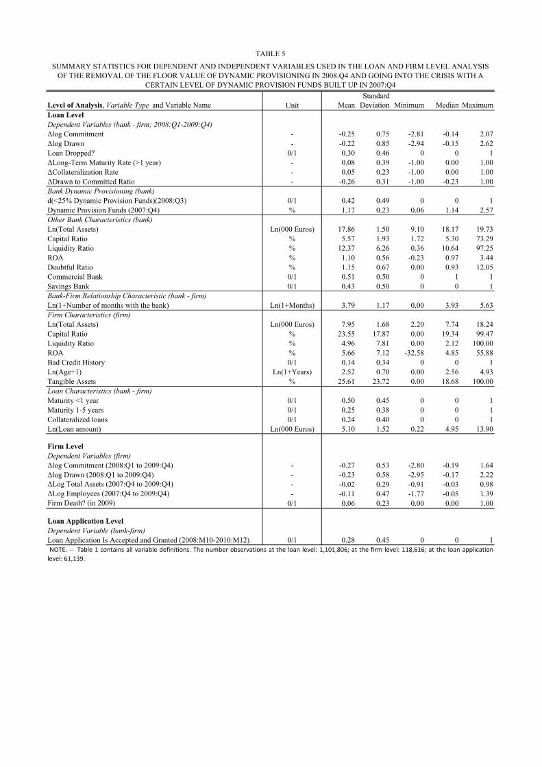
Level of Analysis Variable Type and Variable Name Unit MeanStandard
Deviation Minimum Median MaximumLoan LevelDependent Variables (bank - firm 2008Q1-2009Q4)ǻlog Commitment - -025 075 -281 -014 207ǻlog Drawn - -022 085 -294 -015 262Loan Dropped 01 030 046 0 0 1ǻLong-Term Maturity Rate (gt1 year) - 008 039 -100 000 100ǻCollateralization Rate - 005 023 -100 000 100ǻDrawn to Committed Ratio - -026 031 -100 -023 100Bank Dynamic Provisioning (bank)d(lt25 Dynamic Provision Funds)(2008Q3) 01 042 049 0 0 1Dynamic Provision Funds (2007Q4) 117 023 006 114 257Other Bank Characteristics (bank)Ln(Total Assets) Ln(000 Euros) 1786 150 910 1817 1973Capital Ratio 557 193 172 530 7329Liquidity Ratio 1237 626 036 1064 9725ROA 110 056 -023 097 344Doubtful Ratio 115 067 000 093 1205Commercial Bank 01 051 050 0 1 1Savings Bank 01 043 050 0 0 1Bank-Firm Relationship Characteristic (bank - firm)Ln(1+Number of months with the bank) Ln(1+Months) 379 117 000 393 563Firm Characteristics (firm)Ln(Total Assets) Ln(000 Euros) 795 168 220 774 1824Capital Ratio 2355 1787 000 1934 9947Liquidity Ratio 496 781 000 212 10000ROA 566 712 -3258 485 5588Bad Credit History 01 014 034 0 0 1Ln(Age+1) Ln(1+Years) 252 070 000 256 493Tangible Assets 2561 2372 000 1868 10000Loan Characteristics (bank - firm)Maturity lt1 year 01 050 045 0 0 1Maturity 1-5 years 01 025 038 0 0 1Collateralized loans 01 024 040 0 0 1Ln(Loan amount) Ln(000 Euros) 510 152 022 495 1390
Firm LevelDependent Variables (firm)ǻlog Commitment (2008Q1 to 2009Q4) - -027 053 -280 -019 164ǻlog Drawn (2008Q1 to 2009Q4) - -023 058 -295 -017 222ǻLog Total Assets (2007Q4 to 2009Q4) - -002 029 -091 -003 098ǻLog Employees (2007Q4 to 2009Q4) - -011 047 -177 -005 139Firm Death (in 2009) 01 006 023 000 000 100
Loan Application LevelDependent Variable (bank-firm)Loan Application Is Accepted and Granted (2008M10-2010M12) 01 028 045 0 0 1
TABLE 5
SUMMARY STATISTICS FOR DEPENDENT AND INDEPENDENT VARIABLES USED IN THE LOAN AND FIRM LEVEL ANALYSIS OF THE REMOVAL OF THE FLOOR VALUE OF DYNAMIC PROVISIONING IN 2008Q4 AND GOING INTO THE CRISIS WITH A
CERTAIN LEVEL OF DYNAMIC PROVISION FUNDS BUILT UP IN 2007Q4
NOTE ͲͲ Table 1 contains all variable definitions The number observations at the loan level 1101806 at the firm level 118616 at the loan applicationlevel61139
Model (1) (2) (3) (4) (5) (6) (7) (8) (9) (10) (11)Level
Dep
ende
nt V
aria
ble
ǻlog
Com
mitm
ent
(200
8Q
1-20
09Q
4)
ǻlog
Com
mitm
ent
(200
8Q
1-20
09Q
4)
ǻlog
Com
mitm
ent
(200
8Q
1-20
09Q
4)
ǻlog
Com
mitm
ent
(200
8Q
1-20
09Q
4)
ǻlog
Com
mitm
ent
(200
8Q
1-20
09Q
4)
ǻlog
Com
mitm
ent
(200
8Q
1-20
09Q
4)
ǻlog
Com
mitm
ent
(200
8Q
1-20
09Q
4)
2-St
age
Leas
t Sq
uare
s ǻl
og
Com
mitm
ent
(200
8Q
1-20
09Q
4)
ǻlog
Dra
wn
(200
8Q
1-20
09Q
4)
Loan
Dro
pped
Loan
Dro
pped
d(lt25 Dynamic Provision Funds)(2008Q3)b 0070 0077 0086 0094 0098 0096 0100 0086 0100 -0046 -0038
( 023) ( 028) ( 028) ( 026) ( 024) ( 03) ( 031) ( 029) ( 029) ( 014) ( 014)Dynamic Provision Funds (2007Q4)b 0096 0144 0130 0160 0172 0201 0191 0450 0198 -0054 -0057
( 05) ( 066) ( 066) ( 059) ( 058) ( 069) ( 07) ( 101) ( 061) ( 03) ( 03)Other Bank Characteristics Yes Yes Yes Yes Yes Yes Yes Yes Yes Yes YesBank-Firm Relationship Characteristic Yes Yes Yes Yes Yes Yes Yes Yes Yes Yes YesLoan Characteristics No No No No Yes No No No No No YesProvince and Industry Fixed effects Yes Yes Yes -- -- -- -- -- -- -- --Firm Fixed effects No No No Yes Yes Yes -- -- -- Yes YesFirm Bank Type Fixed Effects No No No No No No Yes Yes Yes No NoSample with Multiple Bank-Firm Relationships Only No No Yes Yes Yes Yes Yes Yes Yes Yes YesSample with Firm Characteristics Only No Yes No No No Yes No No No No NoCluster Bank Bank Bank Bank Bank Bank Bank Bank Bank Bank BankNumber of Observations 1101806 510582 687408 687408 687408 379821 687408 687408 622824 1018699 1018699
Model (12) (13) (14) (15) (16) (17) (18) (19) (20)
Level
Dep
ende
nt V
aria
ble
ǻLon
g-Te
rm M
atur
ity R
ate
(gt1
year
)
(200
8Q
1-20
09Q
4)
ǻCol
late
raliz
atio
n R
ate
(200
8Q
1-20
09Q
4)
ǻDra
wn
to C
omm
itted
Rat
io
(200
8Q
1-20
09Q
4)
ǻlog
Com
mitm
ent
(200
8Q
1-20
09Q
4)
ǻlog
Com
mitm
ent
(200
8Q
1-20
09Q
4)
ǻlog
Tot
al A
sset
s
(200
7Q
4-20
09Q
4)
ǻlog
Em
ploy
ees
(200
7Q
4-20
09Q
4)
Firm
Dea
th
(in
2009
)
Loan
App
licat
ion
Is A
ccep
ted
and
Gra
nted
(200
8M
10-2
010
M12
)
d(lt25 Dynamic Provision Funds)(2008Q3)b -0074 0012 0028 0058 0051 0007 -0005 0002 -0056 ( 021) ( 004) ( 007) ( 015) ( 014) ( 004) ( 006) ( 001) ( 015)
Dynamic Provision Funds (2007Q4)b -0175 0031 0013 0105 0111 0025 0027 -0008 0094 ( 047) ( 01) ( 015) ( 036) ( 035) ( 011) ( 014) ( 004) ( 042)
Other Bank Characteristics Yes Yes Yes Yes Yes Yes Yes Yes YesBank-Firm Relationship Characteristic Yes Yes Yes Yes Yes Yes Yes Yes YesFirm Characteristics -- -- -- Yes Yes Yes Yes Yes NoLoan Characteristics Yes Yes Yes No Yes No No No NoProvince and Industry Fixed effects -- -- -- Yes Yes Yes Yes Yes --Firm Fixed Effects Yes Yes Yes gt lt gt lt gt lt gt lt gt lt Firm-TimeSample with Multiple Bank-Firm Relationships Only Yes Yes Yes Yes Yes Yes Yes Yes NoSample with Firm Characteristics Only No No No Yes Yes Yes Yes Yes NoCluster Bank Bank Bank Main Bank Main Bank Main Bank Main Bank Main Bank BankNumber of Observations 687408 687408 687408 118616 118616 79183 71532 149304 61139
LOANANDFIRMLEVELANALYSISOFTHEEFFECTSOFTHEFLOORREMOVALOFDYNAMICPROVISIONINGIN2008Q4ANDOFGOINGINTOTHECRISISWITHACERTAINLEVELOFDYNAMICPROVISIONFUNDSBUILTUPIN2007Q4TABLE6
NOTE ͲͲ Model 6 corresponds to Equation 1 the adjacent text explains Models 1 to 14 In Model 8 in the first stage we regress Dynamic Provision Funds (2007Q4) on the simulated Dynamic Provision Funds (2007Q4) fixing the bank loan portfolio in 2000Q3 Theestimated coefficient equals 0772 (0133) In the second stage the inͲthisͲway instrumented Dynamic Provision Funds (2007Q4) replaces the actual Dynamic Provision Funds (2007Q4) Model 15 corresponds to Equation 2 the adjacent text explains Models 15 to19 Model 20 corresponds to Equation 3 Table 5 contains the list of variables for each set of characteristics and Table 1 the definition of all variables The Ln(Loan Amount) included in the Loan Characteristics is averaged from 2005Q4 to 2007Q1 Coefficients are listedin the first row robust standard errors that are corrected for clustering at the indicated level are reported in the row below in parentheses and the corresponding significance levels are in the adjacent column Yes indicates that the set of characteristics or fixed effectsis included No indicates that the set of characteristics or fixed effects is not included gt lt indicates that the set of fixed effects cannot be included (because the regression is crossͲsectional at the level of the fixed effects) ͲͲ indicates that the indicated set ofcharacteristicsorfixedeffectsarecomprisedinthewiderincludedsetoffixedeffectsSignificantat1significantat5significantat10
Loan
Loan FirmLoan
Application
Model ( 1) ( 2) ( 3) ( 4) ( 5) ( 6)d(lt25 Dynamic Provision Funds)(2008Q3)b [=DPb] -0392 0098 0148 0226 0380
( 229) ( 077) ( 15) ( 045) ( 226)DPb Ln(Total Assetsb) 0032 -0002
( 013) ( 012)DPb Capital Ratiob 0004 0009
( 013) ( 013)DPb ROAb -0050 -0074
( 048) ( 053)DPb Doubtful Ratiob -0125 -0134
( 029) ( 031)DPb Ln(Total Assetsf) -0011 -0011 -0006
( 004) ( 004) ( 003)DPb Capital Ratiof -0001 -0001 -0001
( 0004) ( 0003) ( 0003)DPb ROAf 0000 0000 0001
( 001) ( 001) ( 001)DPb Bad Credit Historyf -0003 0002 0004
( 01) ( 009) ( 009)DPb Ln(1+Number of months with the bank)bf 0005 0005
( 007) ( 006)Dynamic Provision Funds (2007Q4)b [=DPFb] -0285 0147 0256 0399 0166
( 275) ( 125) ( 15) ( 08) ( 414)DPFb Ln(Total Assetsb) 0023 0007
( 016) ( 018)DPFb Capital Ratiob 0009 0004
( 017) ( 016)DPFb ROAb -0026 -0024
( 136) ( 139)DPFb Doubtful Ratiob -0148 -0125
( 033) ( 043)DPFb Ln(Total Assetsf) 0006 0004 -0002
( 01) ( 009) ( 01)DPFb Capital Ratiof 0000 0000 0000
( 001) ( 001) ( 001)DPFb ROAf -0001 -0001 -0001
( 002) ( 001) ( 001)DPFb Bad Credit Historyf -0021 -0033 -0039
( 018) ( 02) ( 02)DFPb Ln(1+Number of months with the bank)bf 0023 0022
( 014) ( 012)Other Bank Characteristics Yes Yes Yes Yes Yes YesBank-Firm Relationship Characteristic Yes Yes Yes Yes Yes YesFirm Fixed effects Yes Yes Yes Yes Yes YesBank Fixed effects No No No No No YesSample with Multiple Bank-Firm Relationships Only Yes Yes Yes Yes Yes YesSample with Firm Characteristics Only Yes Yes Yes Yes Yes YesCluster Bank Firm Bank Firm Bank Firm Bank Firm Bank Firm Bank FirmNumber of Observations 379821 379821 379821 379821 379821 379821NOTE -- The dependent variable is the ǻlog Commitment (2008Q1-2009Q4) Table 5 contains the list of variables for each set of characteristics and Table 1
contains all variable definitions Coefficients are listed in the first row robust standard errors that are corrected for clustering at the indicated level are reported inthe row below in parentheses and the corresponding significance levels are in the adjacent column Yes indicates that the set of characteristics or fixed effects isincluded Significant at 1 significant at 5 significant at 10
ANALYSIS OF THE CHANGES IN COMMITTED LENDING FOLLOWING THE FLOOR REMOVAL OF DYNAMIC PROVISIONING IN 2008Q4 AND OF GOING INTO THE CRISIS WITH A CERTAIN LEVEL OF DYNAMIC PROVISION FUNDS BUILT UP IN 2007Q4 ACROSS BANKS AND FIRMS
TABLE 7
APPENDIX
- FOR ONLINE PUBLICATION -
CALCULATION OF DYNAMIC PROVISIONS
Dynamic provisions are formula based The total loan loss provisions for a period are the
sum of the Specific plus General Provisions The per-period (ie the flow of) General
Provisions are computed as
௧ݏݏݒݎݎܩ ൌ ௧ݏܮοߙ ൬ߚ െ ௧ݏݏݒݎ௧ݏܮ
൰ ௧ (A1)ݏܮ
where Loanst is the stock of loans at the end of period t and Loanst its variation from the end
of period t-1 to the end of period t (positive in a lending expansion negative in a credit
decline) D and E are parameters set by the Banco de Espantildea the Spanish banking regulator
D is an estimate of the percent latent loss in the loan portfolio while E is the average along the
cycle of specific provisions in relative terms Hence the second term is the key counter-
cyclical component
The above formula is in fact a simplification There are six risk buckets or homogeneous
groups of risk to take into account the different nature of the distinct segments of the credit
market each of them with a different D and E parameter These groups (in ascending order of
risk) are the following
i) Negligible risk Includes cash and public-sector exposures (both loans and
securities) as well as interbank exposures
ii) Low risk Made up of mortgages with a loan-to-value (LTV) ratio below 80 and
exposures to corporations with an A or higher rating
iii) Medium-low risk Composed of mortgages with an LTV ratio above 80 and other
collateralized loans not previously mentioned
iv) Medium risk Made up of other loans including unrated or below-A rated corporate
exposures and exposures to small and medium-sized firms
v) Medium-high risk Consumer durables financing and finally
vi) High risk Credit card exposures and overdrafts
The values for D are (moving from lower to higher risk levels) 0 06 15 18 2 and 25
percent and those for E 0 011 044 065 11 and 164 percent These are the parameter
values as they were modified in 2005Q1 (our second policy experiment) after their
introduction in 2000Q3 (our first policy experiment)
The final formula to be applied by each bank is therefore
௧ݏݏݒݎݎܩ
ൌߙοݏܮ௧
ୀଵ൬ߚ െ
௧ݏݏݒݎ௧ݏܮ
൰ ௧ݏܮ
ୀଵ
(A2)
௧ݏݏݒݎݎܩ
ൌߙοݏܮ௧
ୀଵ ൭ߚݏܮ௧
ୀଵെ ௧൱ݏݏݒݎ
(A3)
Moreover there is a ceiling for the fund of general loan loss provisions fixed at 125
percent of the product of parameter Į and the total volume of credit exposures Therefore the
fund of general provisions should be below 125 percent of the latent loss of the loan portfolio
The objective of this ceiling is to avoid an excess of provisioning which might occur in a
long expansionary phase as specific provisions remain below the ȕ component whereas the Į
component contributes positively to the accumulation of provisions in the fund The ceiling is
intended to avoid a provision fund that keeps growing indefinitely producing unnecessarily
too high coverage ratios of non-performing loans
There was also a minimum floor value for the fund of general provisions at 33 percent of
the latent loss This minimum was lowered at the end of 2008 to 10 percent in order to allow
for more usage of the general provisions previously built in the expansionary period (our third
policy experiment)
TAX TREATEMENT OF DYNAMIC PROVISIONS
Regarding tax treatment general provisions are tax-deductible up to 1 percent of the
increase in gross loans as long as they are not mortgages Non-deductible amounts (ie those
above that threshold) are accounted for as deferred tax assets because they will become
specific provisions in the future and therefore deductible when the impairment is assigned to
an individual loan Before 2005 the countercyclical part of the loan loss provisions was not
tax-deductible
FIGUREA1ESTIMATESOFTIMEͲVARYINGCOEFFICIENTONTHEINDEPENDENTVARIABLEDYNAMICPROVISIONFORCOMMITMENTLENDING
NOTE ͲͲ Solid lines represent the coefficients of Dynamic Provision in Models 8 and 17 in Table A2 that are estimated with rolling time windows Dashed lines represent the two standard error confidence band drawn around the coefficient estimates Black lines are at theloanlevelbluelinesareatthefirmlevelTable1containsallvariabledefinitions
Ͳ04
Ͳ03
Ͳ02
Ͳ01
0
01
02
03
04
0520
05Q1
2005Q1
2005Q2
2005Q3
2005Q4
2006Q1
2006Q2
2006Q3
2006Q4
2007Q1
2007Q2
2007Q3
2007Q4
ȴLogCommitment
LoanLevel FirmLevel
Level of Analysis Variable Type and Variable Name Unit MeanStandard
Deviation Minimum Median MaximumLoan LevelDependent Variables (bank - firm 2004Q4-2006Q2)ǻlog Commitment - 001 093 -277 -006 305ǻlog Drawn - 001 080 -252 000 268Loan Dropped 01 026 044 0 0 1ǻLong-Term Maturity Rate (gt1 year) - 000 032 -100 000 100ǻCollateralization Rate - 001 019 -100 000 100ǻDrawn to Committed Ratio - -025 031 -100 -022 100Bank Dynamic Provisioning (bank 2004Q4 to 2005Q2)Dynamic Provision 005 014 -018 000 037Dynamic Provision Funds Latent Risk - 133 018 026 138 205Other Bank Characteristics (bank)Ln(Total Assets) Ln(000 Euros) 1735 155 897 1763 1929Capital Ratio 631 309 178 559 5337Liquidity Ratio 1818 722 003 1835 8913ROA 094 050 -323 089 563Doubtful Ratio 066 040 000 055 5356Commercial Bank 01 054 050 0 1 1Savings Bank 01 040 049 0 0 1Bank-Firm Relationship Characteristic (bank - firm)Ln(1+Number of months with the bank) Ln(1+Months) 376 117 000 395 548Firm Characteristics (firm)Ln(Total Assets) Ln(000 Euros) 749 165 161 730 1771Capital Ratio 2460 1797 001 2074 9957Liquidity Ratio 597 871 000 286 10000ROA 613 776 -3548 517 6316Bad Credit History 01 013 034 0 0 1Ln(Age+1) Ln(1+Years) 235 078 000 240 490Tangible Assets 2613 2332 000 1966 10000Loan Characteristics (bank - firm)Maturity lt1 year 01 055 044 0 1 1Maturity 1-5 years 01 024 037 0 0 1Collateralized Loan 01 019 037 0 0 1Ln(Loan Amount) Ln(000 Euros) 460 174 000 460 1358
Firm LevelDependent Variables (firm ) -ǻlog Commitment (2004Q4-2006Q2) - -001 058 -259 -003 236ǻlog Drawn (2004Q4-2006Q2) - -001 064 -278 -004 270ǻlog Total Assets (2004Q4-2006Q4) - 017 038 -092 011 165ǻlog Employees (2004Q4-2006Q4) - 007 041 -139 000 161Firm Death (2006) 01 002 015 0 0 1
Loan Application LevelDependent Variable (bank-firm 2005M7-2006M12)Loan Application Is Accepted and Granted 01 040 049 0 0 1
TABLE A1SUMMARY STATISTICS FOR DEPENDENT AND INDEPENDENT VARIABLES USED IN THE LOAN AND FIRM LEVEL ANALYSIS OF
THE MODIFICATION OF DYNAMIC PROVISIONING IN 2005Q1
NOTE -- Table 1 contains all variable definitions The number observations at the loan level 884859 at the firm level 107087 at the loanapplication level 71050
Model (1) (2) (3) (4) (5) (6) (7) (8) (9) (10)Level
Dep
ende
nt V
aria
ble
ǻlog
Com
mitm
ent
(200
4Q
4-20
06Q
2)
ǻlog
Com
mitm
ent
(200
4Q
4-20
06Q
2)
ǻlog
Com
mitm
ent
(200
4Q
4-20
06Q
2)
ǻlog
Com
mitm
ent
(200
4Q
4-20
06Q
2)
ǻlog
Com
mitm
ent
(200
4Q
4-20
06Q
2)
ǻlog
Com
mitm
ent
(200
4Q
4-20
06Q
2)
ǻlog
Com
mitm
ent
(200
4Q
4-20
06Q
2)
ǻlog
Dra
wn
(200
0Q
1-20
01Q
2)
Loan
Dro
pped
Loan
Dro
pped
Dynamic Provision(2004Q4-2005Q2)b -0111 -0120 -0124 -0108 -0040 -0115 -0045 -0100 0033 0046( 047) ( 054) ( 056) ( 048) ( 049) ( 048) ( 053) ( 0563) ( 037) ( 037)
Other Bank Characteristics Yes Yes Yes Yes Yes Yes Yes Yes Yes YesBank-Firm Relationship Characteristic Yes Yes Yes Yes Yes Yes Yes Yes Yes YesLoan Characteristics No No No No Yes No No No No YesProvince and Industry Fixed effects Yes Yes Yes -- -- -- -- -- -- --Firm Fixed Effects No No No Yes Yes Yes -- -- Yes YesFirm Bank Type Fixed Effects No No No No No No Yes Yes No NoSample with Multiple Bank-Firm Relationships Only No No Yes Yes Yes Yes Yes Yes YesSample with Firm Characteristics Only No Yes No No No Yes No No No NoCluster Bank Bank Bank Bank Bank Bank Bank Bank Bank BankNumber of Observations 884859 460885 543499 543499 543499 334631 543499 480359 750735 750735
Model (11) (12) (13) (14) (15) (16) (17) (18) (19)
Level
Dep
ende
nt V
aria
ble
ǻLon
g-Te
rm M
atur
ity R
ate
(gt1
year
)
(200
4Q
4-20
06Q
2)
ǻCol
late
raliz
atio
n R
ate
(200
4Q
4-20
06Q
2)
ǻDra
wn
to C
omm
itted
Rat
io
(200
4Q
4-20
06Q
2)
ǻlog
Com
mitm
ent
(200
4Q
4-20
06Q
2)
ǻlog
Com
mitm
ent
(200
4Q
4-20
06Q
2)
ǻlog
Tot
al A
sset
s
(200
4Q
4-20
06Q
4)
ǻlog
Em
ploy
ees
(200
4Q
4-20
06Q
4)
Firm
Dea
th
(in
2006
)
Loan
App
licat
ion
Is A
ccep
ted
and
Gra
nted
(200
5M
7-20
06M
12)
Dynamic Provision(2004Q4-2005Q2)b -0065 0022 0009 -0074 -0039 0003 0014 -0004 -0003( 064) ( 011) ( 057) ( 038) ( 033) ( 02) ( 022) ( 006) ( 046)
Other Bank Characteristics Yes Yes Yes Yes Yes Yes Yes Yes YesBank-Firm Relationship Characteristic Yes Yes Yes Yes Yes Yes Yes Yes YesFirm Characteristics -- -- -- Yes Yes Yes Yes Yes NoLoan Characteristics Yes Yes Yes No Yes No No No NoProvince and Industry Fixed effects -- -- -- Yes Yes Yes Yes Yes --Firm Fixed Effects Yes Yes Yes gt lt gt lt gt lt gt lt gt lt Firm-TimeSample with Multiple Bank-Firm Relationships Only Yes Yes Yes Yes Yes Yes Yes Yes NoSample with Firm Characteristics Only No No No Yes Yes Yes Yes Yes NoCluster Bank Bank Bank Main Bank Main Bank Main Bank Main Bank Main Bank BankNumber of Observations 543499 543499 327233 107087 107087 79877 68737 132634 71050
LOAN AND FIRM LEVEL ANALYSIS OF THE EFFECTS OF THE MODIFICATION OF DYNAMIC PROVISIONING IN 2005Q1
Loan
Loan
FirmLoan
Application
TABLE A2
NOTE -- Model 6 corresponds to Equation 1 the adjacent text explains Models 1 to 13 Model 14 corresponds to Equation 2 the adjacent text explains Models 14 to 18 Model 19 corresponds to Equation 3 The instrumentation ofDynamic Provision is explained in Equation 3 and adjacent text Table A1 contains the list of variables for each set of characteristics and Table 1 the definition of all variables The Ln(Loan Amount) included in the LoanCharacteristics is averaged from 2004Q4 to 2005Q4 Coefficients are listed in the first row robust standard errors that are corrected for clustering at the indicated level are reported in the row below in parentheses and thecorresponding significance levels are in the adjacent column Yes indicates that the set of characteristics or fixed effects is included No indicates that the set of characteristics or fixed effects is not included gt lt indicates thatthe set of fixed effects cannot be included (because the regression is cross-sectional at the level of the fixed effects) -- indicates that the indicated set of characteristics or fixed effects are comprised in the wider included set of fixedeffects Significant at 1 significant at 5 significant at 10
Model ( 1) ( 2) ( 3) ( 4) ( 5) ( 5)Dynamic Provision(2004Q4-2005Q2)b [=DPb] -1986 0133 -0135 0159 -4736
( 658) ( 323) ( 15) ( 716) ( 16505)DPb Ln(Total Assetsb) 0108 0249
( 039) ( 778)DPb Capital Ratiob -0039 -0037
( 051) ( 186)DPb ROAb 0035 -0172
( 1) ( 324)DPb Doubtful Ratiob -0394 0955
( 1063) ( 6099)DPb Ln(Total Assetsf) 0010 0018 0002
( 015) ( 068) ( 015)DPb Capital Ratiof -0001 -0001 -0001
( 002) ( 003) ( 002)DPb ROAf -0002 -0002 -0002
( 002) ( 002) ( 002)DPb Bad Credit Historyf -0028 -0024 -0024
( 05) ( 099) ( 036)DPb Ln(1+Number of months with the bank)bf 0024 0004
( 038) ( 013)Other Bank Characteristics Yes Yes Yes Yes Yes YesBank-Firm Relationship Characteristic Yes Yes Yes Yes Yes YesFirm Fixed effects Yes Yes Yes Yes Yes YesBank Fixed effects No No No No No YesSample with Multiple Bank-Firm Relationships Only Yes Yes Yes Yes Yes YesSample with Firm Characteristics Only Yes Yes Yes Yes Yes YesCluster Bank Firm Bank Firm Bank Firm Bank Firm Bank Firm Bank FirmNumber of Observations 334631 334631 334631 334631 334631 334631NOTE -- The dependent variable is the ǻlog Commitment (2004Q4-2006Q2) Table A1 contains the list of variables for each set of characteristics and Table 1
contains all variable definitions Coefficients are listed in the first row robust standard errors that are corrected for clustering at the indicated level are reported in therow below in parentheses and the corresponding significance levels are in the adjacent column Yes indicates that the set of characteristics or fixed effects isincluded Significant at 1 significant at 5 significant at 10
ANALYSIS OF THE CHANGES IN COMMITTED LENDING AT THE MODIFICATION OF DYNAMIC PROVISIONING IN 2005Q1 ACROSS BANKS AND FIRMS
TABLE A3
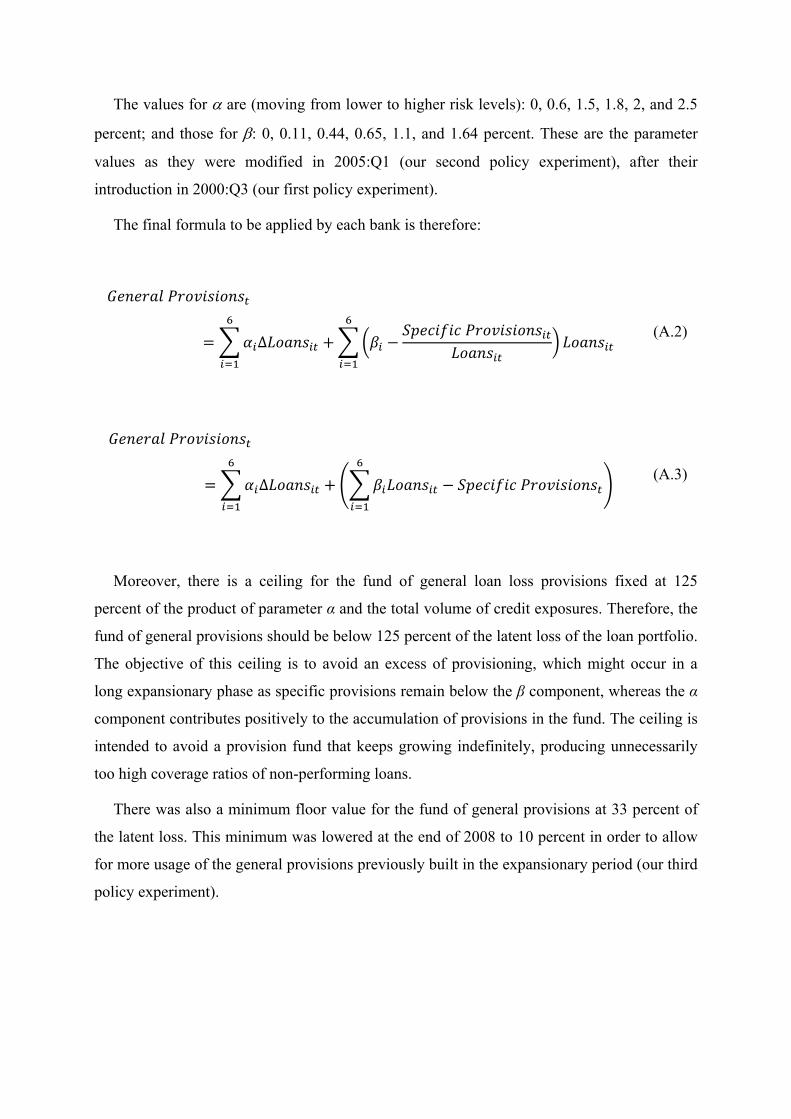
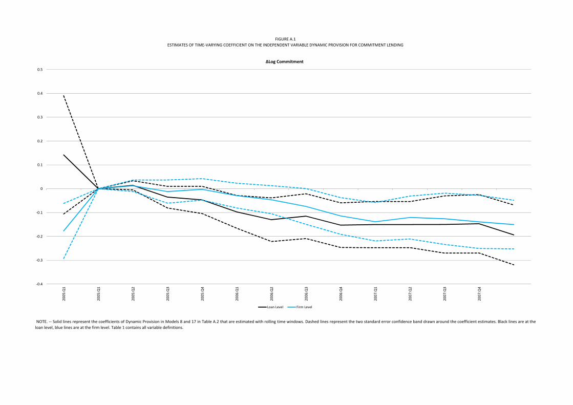