Macroeconomics and ARCH*

James D. Hamilton

Department of Economics

University of California, San Diego

jhamilton@ucsd.edu

September 24, 2007

Revised: May 27, 2008

*Prepared for the Festschrift in Honor of Robert F. Engle (eds. Tim Bollerslev, Jeffrey

R. Russell and Mark Watson).

Abstract

Although ARCH-related models have proven quite popular in finance, they are less fre-

quently used in macroeconomic applications. In part this may be because macroeconomists

are usually more concerned about characterizing the conditional mean rather than the con-

ditional variance of a time series. This paper argues that even if one’s interest is in the

conditional mean, correctly modeling the conditional variance can still be quite important,

for two reasons. First, OLS standard errors can be quite misleading, with a “spurious regres-

sion” possibility in which a true null hypothesis is asymptotically rejected with probability

one. Second, the inference about the conditional mean can be inappropriately influenced by

outliers and high-variance episodes if one has not incorporated the conditional variance di-

rectly into the estimation of the mean, and infinite relative efficiency gains may be possible.

The practical relevance of these concerns is illustrated with two empirical examples from

the macroeconomics literature, the first looking at market expectations of future changes in

Federal Reserve policy, and the second looking at changes over time in the Fed’s adherence

to a Taylor Rule.

1

1 Introduction.

One of the most influential econometric papers of the last generation was Engle’s (1982a)

introduction of autoregressive conditional heteroskedasticity (ARCH) as a tool for describing

how the conditional variance of a time series evolves over time. The ISI Web of Science lists

over 2000 academic studies that have cited this article, and simply reciting the acronyms

for the various extensions of Engle’s theme involves a not insignificant commitment of paper

(see Table 1, or the more detailed glossary in Bollerslev, 2008).

The vast majority of empirical applications of ARCH models have studied financial time

series such as stock prices, interest rates, or exchange rates. To be sure, there have also

been a number of interesting applications of ARCH to macroeconomic questions. Lee, Ni,

and Ratti (1995) noted that the conditional volatility of oil prices, as captured by a GARCH

model, seems to matter for the magnitude of the effect on GDP of a given movement in

oil prices, and Elder and Serletis (2006) use a vector autoregression with GARCH-in-mean

elements to describe the direct consequences of oil-price volatility for GDP. Grier and Perry

(2000) and Fountas and Karanasos (2007) use such models to conclude that inflation and

output volatility also can depress real GDP growth, while Servén (2003) studied the effects

of uncertainty on investment spending.

However, despite these interesting applications, studying volatility has traditionally been

a much lower priority for macroeconomists than for researchers in financial markets because

the former’s interest is primarily in describing the first moments. There seems to be an as-

sumption among many macroeconomists that, if your primary interest is in the first moment,

2

ARCH has little relevance apart from possible GARCH-M effects.

The purpose of this paper is to suggest that even if our primary interest is in estimating

the conditional mean, having a correct description of the conditional variance can still be

quite important, for two reasons. First, hypothesis tests about the mean in a model in

which the variance is misspecified will be invalid. Second, by incorporating the observed

features of the heteroskedasticity into the estimation of the conditional mean, substantially

more efficient estimates of the conditional mean can be obtained.

Section 2 develops the theoretical basis for these claims, illustrating the potential magni-

tude of the problem with a small Monte Carlo study and explaining why the popular White

(1980) or Newey-West (1987) corrections may not fully correct for the inference problems

introduced by ARCH. The subsequent sections illustrate the practical relevance of these

concerns using two examples from the macroeconomics literature. The first application

concerns measures of what the market expects the U.S. Federal Reserve’s next move to

be, and the second explores the extent to which U.S. monetary policy today is following a

fundamentally different rule from that observed thirty years ago.

I recognize that it may require more than these limited examples to persuade macro-

economists to pay more attention to ARCH. Another thing I learned from Rob Engle is

that, in addition to coming up with a great idea, it doesn’t hurt if you also have a catchy

acronym that people can use to describe what you’re talking about. After all, where would

we be today if we all had to pronounce “autoregressive conditional heteroskedasticity” every

time we wanted to discuss these issues? However, Table 1 reveals that the acronyms one

3

might logically use for “Macroeconomics and ARCH” seem already to be taken. “MARCH”,

for example, is already used (twice), as is “ARCH-M”.

Fortunately, Engle and Manganelli (2004) have shown us that it’s also OK to mix upper-

and lower-case letters, picking and choosing handy vowels or consonants so as to come up

with something catchy, as in “CAViaR” (Conditional Autoregressive Value at Risk). In

that spirit, I propose to designate “Macroeconomics and ARCH” as “McARCH.” Maybe

not a new product so much as new packaging.

Herewith, then, discussion of the relevance of McARCH.

2 GARCH and inference about the mean.

We can illustrate some of the issues with the following simple model:

yt = β0 + β1yt−1 + ut (1)

ut =phtvt (2)

ht = κ+ αu2t−1 + δht−1 for t = 1, 2, ..., T

h0 = κ/(1− α− δ)

vt ∼ i.i.d. N(0, 1). (3)

Bollerslev (1986, pp. 312-313) showed that if

3α2 + 2αδ + δ2 < 1, (4)

4

then the noncentral unconditional second and fourth moments of ut exist and are given by

µ2 = E(u2t ) =

κ

1− α− δ(5)

µ4 = E(u4t ) =

3κ2(1 + α+ δ)

(1− α− δ)(1− δ2 − 2αδ − 3α2) . (6)

Consider the consequences if the mean parameters β0 and β1 are estimated by ordinary least

squares,

β =³X

xtx0t

´−1 ³Xxtyt

´β = (β0,β1)

0

xt = (1, yt−1)0,

and where all summations are for t = 1, ..., T. Suppose further that inference is based on

the usual OLS formula for the variance, with no correction for heteroskedasticity:

V = s2³X

xtx0t

´−1(7)

s2 = (T − 2)−1X

u2t

ut = yt − x0tβ

Consider first the consequences of this inference when the fourth-moment condition (4)

is satisfied. For simplicity of exposition, consider the case when the true value of β = 0.

Then from the standard consistency results (e.g., Lee and Hansen, 1994; Lumsdaine, 1996)

5

we see that

T V = s2³T−1

Xxtx

0t

´−1(8)

p→ E(u2t )

1 E(yt−1)

E(yt−1) E(y2t−1)

−1

=

µ2 0

0 1

−1

.

In other words, the OLS formulas will lead us to act as if√T β1 is approximately N(0, 1) if

the true value of β1 is zero. But notice

√T (β − β) =

³T−1

Xxtx

0t

´−1 ³T−1/2

Xxtut

´. (9)

Under the null hypothesis, the term inside the second summation, xtut, is a martingale

difference sequence with variance

E(u2txtx0t) =

E(u2t ) E(u2tut−1)

E(ut−1u2t ) E(u2tu2t−1)

.When the (2,2) element of this matrix is finite, it then follows from the Central Limit

Theorem (e.g., Hamilton, 1994, p. 173) that

T−1/2X

yt−1utL→ N

¡0, E

¡u2tu

2t−1¢¢. (10)

To calculate the value of this variance, recall (e.g., Hamilton, 1994, p. 666) that the

GARCH(1,1) structure for ut implies an ARMA(1,1) structure for u2t :

u2t = κ+ (δ + α)u2t−1 + wt − δwt−1

6

for wt−1 a white noise process. It follows from the first-order autocovariance for an

ARMA(1,1) process (e.g., Box and Jenkins, 1976, p. 76) that

E(u2tu2t−1) = E(u2t − µ2)(u2t−1 − µ2) + µ22

= ρ(µ4 − µ22) + µ22 (11)

for

ρ =[1− (α+ δ)δ]α

1 + δ2 − 2(α+ δ)δ. (12)

Substituting (11), (10) and (8) into (9),

√T β1

L→ N(0, V11)

V11 =ρµ4 + (1− ρ)µ22

µ22

= ρ3(1 + α+ δ)(1− α− δ)

(1− δ2 − 2αδ − 3α2) + (1− ρ).

with the last equality following from (5) and (6).

Notice that V11 ≥ 1, with equality if and only if α = 0. Thus OLS treats√T β1 as

approximately N(0, 1), whereas the true asymptotic distribution is Normal with a variance

bigger than unity, meaning that the OLS t test will systematically reject more often than it

should. The probability of rejecting the null hypothesis that β1 = 0 (even though the null

hypothesis is true) gets bigger and bigger as the parameters get closer to the region at which

the fourth moment becomes infinite, at which point the asymptotic rejection probability

becomes unity. Figure 1 plots the rejection probability as a function of a and δ. If these

parameters are in the range typically found in estimates of GARCH processes, an OLS t

7

test with no correction for heteroskedasticity would spuriously reject with arbitrarily high

probability for a sufficiently large sample.

The good news is that the rate of divergence is pretty slow— it may take a lot of obser-

vations before the accumulated excess kurtosis overwhelms the other factors. I simulated

10,000 samples from the above Gaussian GARCH process for samples of size T = 100, 200,

and 1000 and 10,000, (and 1,000 samples of size 100,000), where the true values were specified

as follows:

β0 = β1 = 0

κ = 2

α = 0.35

δ = 0.6.

The solid line in Figure 2 plots the fraction of samples for which an OLS t test of β1 = 0

exceeds two in absolute value. Thinking we’re only rejecting a true null hypothesis 5% of

the time, we would in fact do so 15% of the time in a sample of size T = 100 and 33% of

the time when T = 1, 000.

As one might imagine, for a given sample size, the OLS t-statistic is more poorly behaved

if the true innovations vt in (2) are Student’s t with 5 degrees of freedom (the dashed line

in Figure 2) rather than Normal.

What happens if instead of the OLS formula (7) for the variance of β we use White’s

8

(1980) heteroskedasticity-consistent estimate,

V =³X

xtx0t

´−1 ³Xu2txtx

0t

´³Xxtx

0t

´−1? (13)

ARCH is not a special case of the class of heteroskedasticity for which V is intended to be

robust, and indeed, unlike typical cases, T V is not a consistent estimate of a given matrix:

T V =³T−1

Xxtx

0t

´−1 ³T−1

Xu2txtx

0t

´³T−1

Xxtx

0t

´−1.

The first and last matrices will converge as before,

T−1X

xtx0t

p→

1 0

0 µ2

,but T−1

Pu2txtx

0t will diverge if the fourth moment µ4 is infinite. Figure 3 plots the simu-

lated value for the square root of the lower-right element of T V for the Gaussian simulations

above. However, this growth in the estimated variance of√T β1 is exactly right, given

the growth of the actual variance of√T β1 implied by the GARCH specification. And a

t test based on (13) seems to perform reasonably well for all sample sizes (see the second

row of Table 2). The small-sample size distortion for the White test is a little worse for

Student’s t compared with Normal errors, though still acceptable. Table 2 also explores the

consequences of using the Newey-West (1987) generalization of the White formula to allow

for serial correlation, using a lag window of q = 5:

V∗=

ÃTXt=1

xtx0t

!−1 "(1− v

q + 1)

TXt=v+1

utut−v³xtx

0t−v + xt−vx

0t

´#Ã TXt=1

xtx0t

!−1.

These results (reported in the third row of the two panels of Table 2) illustrate one potential

pitfall of relying too much on “robust” statistics to solve the small-sample problems, in that

9

it has more serious size distortions than does the simple White statistic for all specifications

investigated.

Another reason one might not want to assume that White or Newey-West standard errors

can solve all the problems is that these formulas only correct the standard error for β, but are

still using the OLS estimate itself, which from Figure 3 was seen not to be√T convergent.

By contrast, even if the fourth moment does not exist, maximum likelihood estimation as an

alternative to OLS is still√T convergent. Hence the relative efficiency gains of MLE relative

to OLS become infinite as the sample size grows for typical values of GARCH parameters.

Engle (1982, p. 999) observed that it is also possible to have an infinite relative efficiency

gain for some parameter values even with exogenous explanatory variables and ARCH as

opposed to GARCH errors.

Results here are also related to the well-known result that ARCH will render inaccurate

traditional tests for serial correlation in the mean. That fact has previously been noted,

for example, by Milhøj (1985, 1987), Diebold (1988), Stambaugh (1993), and Bollerslev and

Mikkelsen (1996). However, none of the above seems to have commented on the fact (though

it is implied by the formulas they use) that the test size goes to unity as the fourth moment

approaches infinity, or noted the implications as here for OLS regression.

Finally, I observe that just checking for a difference between the OLS and the White

standard errors will sometimes not be sufficient to detect these problems. The difference

between V and V will be governed by the size of

X(s2 − u2t )xtx

0t.

10

White (1980) suggested a formal test of whether this magnitude is sufficiently small on the

basis of an OLS regression of u2t on the vector ψt consisting of the unique elements of xtx0t.

In the present case, ψt = (1, yt−1, y2t−1)

0. White showed that, under the null hypothesis that

the OLS standard errors are correct, TR2 from a regression of u2t on ψt would have a χ2(2)

distribution. The next-to-last row of each panel of Table 2 reports the fraction of samples

for which this test would (correctly) reject the null hypothesis. It would miss about half the

time in a sample as small as 100 observations but is more reliable for larger sample sizes.

Alternatively, one can look at Engle’s (1982) analogous test for the null of homoskedas-

ticity against the alternative of qth-order ARCH by looking at TR2 from a regression of

u2t on (1, u2t−1, u

2t−2, ..., u

2t−q)

0, which asymptotically has a χ2(q) distribution under the null.

The last rows in Table 2 report the rejection frequency for this test using q = 3 lags. Not

surprisingly, since this test is designed specifically for the ARCH class of alternatives whereas

the White test is not, this test has a little more power. Its advantage over the White test

for homoskedasticity is presumably greater in many macro applications in which xt includes

a number of variables and their lags, in which case the vector ψt can become unwieldy,

whereas the Engle test remains a simple χ2(q) regardless of the size of xt.

The philosophy of McARCH, then, is quite simple. The Engle TR2 diagnostic should

be calculated routinely in any macroeconomic analysis. If a violation of homoskedasticity is

found, one should compare the OLS estimates with maximum likelihood to make sure that

the inference is robust. The following sections illustrate the potential importance of doing

so with two examples from applied macroeconomics.

11

3 Application 1: Measuring market expectations of

what the Federal Reserve is going to do next.

My first example is adapted from Hamilton (forthcoming). The fed funds rate is a market-

determined interest rates at which banks lend reserves to one another overnight. This

interest rate is extremely sensitive to the supply of reserves created by the Fed, and in

recent years monetary policy has been implemented in terms of a clearly announced target

for the fed funds rate that the Fed intends to achieve.

A critical factor that determines how Fed actions affect the economy is expectations by

the public as to what the Fed is going to do next, as discussed, for example, in my (2008)

paper. One natural place to look for an indication of what those expectations might be is

the fed funds futures market.

Let t = 1, 2, .., T index monthly observations. In the empirical results reported here,

t = 1 corresponds to October, 1988 and the last observation (T = 213) is June 2006. For

each month, we’re interested in what the market expects for the average effective fed funds

rate over that month, denoted rt. For the empirical estimates reported in this section, rt

is measured in basis points, so that for example rt = 525 corresponds to an annual interest

rate of 5.25%.

On any business day, one can enter into a futures contract through the Chicago Board of

Trade whose settlement is based on what the value of rt+j actually turns out to be for some

future month. The terms of a j-month-ahead contract traded on the last day of month t can

12

be translated1 into an interest rate f (j)t such that, if rt+j turns out to be less than f(j)t , then

the seller of the contract has to compensate the buyer a certain amount (specifically, $41.67

on a standard contract) for every basis point by which f (j)t exceeds rt+j. If f(j)t < rt+j, the

buyer pays the seller. Since f (j)t is known as of the end of month t but rt+j will not be

known until the end of month t+ j, the buyer of the contract is basically making a bet that

rt+j will be less than f(j)t . If the marginal market participant were risk neutral, it would be

the case that

f(j)t = Et(rt+j) (14)

where Et(.) denotes the mathematical expectation on the basis of any information publicly

available as of the last day of month t. If (14) holds, we could just look at the value of f (j)t

to infer what market participants expect the Federal Reserve to do in the coming months.

However, previous investigators such as Sack (2004) and Piazzesi and Swanson (forth-

coming) have concluded that (14) does not hold. The simplest way to investigate this claim

is to construct the forecast error implied by the 1-month-ahead contract,

u(1)t = rt − f (1)t−1

and test whether this error indeed has mean zero, as it should if (14) were correct. For

contracts at longer horizons j > 1, one can look at the monthly change in contract terms,

u(j)t = f

(j−1)t − f (j)t−1.

1 Specifically, if Pt is the price of the contract agreed to by the buyer and seller on day t, then ft =100× (100− Pt).

13

If (14) holds, then u(j)t would also be a martingale difference sequence:

u(j)t = Et(rt+j−1)−Et−1(rt+j−1).

One simple test is then to perform the regression

u(j)t = µ(j) + ε

(j)t

and test the null hypothesis that µ(j) = 0; this is of course just the usual t-test for a sample

mean. Table 3 reports the results of this test using 1-, 2-, and 3-month-ahead futures

contracts. For the historical sample, the 1-month-ahead futures contract f (1)t overestimated

the value of rt+1 by an average of 2.66 basis points and f(j)t overestimated the value of f (j−1)t+1

by almost 4 basis points. One interpretation is that there is a risk premium built into these

contracts. Another possibility is that the market participants failed to recognize fully the

chronic decline in interest rates over this period.

Before putting too much credence in such interpretations, however, recall that the theory

(14) implies that u(j)t should be a martingale difference sequence but makes no claims about

predictability of its variance. Figure 4 reveals that each of the series u(j)t exhibits some

clustering of volatility and a significant decline in variability over time, in addition to occa-

sional very large outliers. Engle’s TR2 test for omitted 4th-order ARCH finds very strong

evidence of conditional heteroskedasticity at least for u(1)t and u(3)t ; see Table 3. Hence if we

are interested in a more accurate estimate of the bias and statistical test of its significance,

we might want to model these features of the data.

Hamilton (forthcoming) calculated maximum likelihood estimates for parameters of the

14

following EGARCH specification (with (j) superscripts on all variables and parameters sup-

pressed for ease of readability):

ut = µ+phtεt (15)

log ht − γ 0zt = α(|εt−1|− k2) + δ(log ht−1 − γ 0zt−1) (16)

zt = (1, t/1000)0

k2 = E|εt| = 2√νΓ[(ν + 1)/2]

(ν − 1)√πΓ(ν/2)

for εt a Student’s t variable with ν degrees of freedom and Γ(.) the gamma function:

Γ(s) =

Z ∞

0

xs−1e−x dx.

The log likelihood is then found from

TXt=1

log f(ut|Ut−1;θ) (17)

f(ut|Ut−1,θ) =³k1/pht

´[1 + (ε2t/ν)]

−(ν+1)/2

k1 = Γ[(ν + 1)/2]/[Γ(ν/2)√νπ].

Given numerical values for the parameter vector θ = (µ,γ 0,α, δ, ν)0 and observed data

UT = (u1, u2, ..., uT )0 we can then begin the iteration (16) for t = 1 by setting h1 = exp(γ 0z0).

Plugging this into (15) gives us a value for ε1, which from (16) gives us the number for h2.

Iterating in this fashion gives the sequence {ht, εt}Tt=1 from which the log likelihood (17)

can be evaluated for the specified numerical value of θ. One then tries another guess for θ

in order to numerically maximize the likelihood function. Asymptotic standard errors can

15

be obtained from numerical second derivatives of the log likelihood as in Hamilton (1994,

equation [5.8.3]).

Maximum likelihood parameter estimates are reported in Table 4. Adding these features

provides an overwhelming improvement in fit, with a likelihood ratio test statistic well in

excess of 100 when adding just 4 parameters to a simple Gaussian specification with constant

variance. The very low estimated degrees of freedom results from the big outliers in the

data, and both the serial dependence (δ) and trend parameter (γ2) for the variance are

extremely significant.

A very remarkable result is that the estimates for the mean of the forecast error µ actually

switch signs, shrink by an order of magnitude, and become far from statistically significant.

Evidently the sample means of u(j)t are more influenced by negative outliers and observations

early in the sample than they should be.

Note that for this example, the problem is not adequately addressed by simply replacing

OLS standard errors with White standard errors, since when the regressors consist only

of a constant term, the two would be identical. Moreover, whenever, as here, there is

an affirmative objective of obtaining accurate estimates of a parameter (the possible risk

premium incorporated in these prices) as opposed solely to testing a hypothesis, the concern

is with the quality of the coefficient estimate itself rather than the correct size of a hypothesis

test.

16

4 Application 2: Using the Taylor Rule to summarizechanges in Federal Reserve policy.

One of the most influential papers for both macroeconomic research and policy over the last

decade has been John Taylor’s (1993) proposal of a simple rule that the central bank should

follow in setting an interest rate like the fed funds rate rt. Taylor’s proposal called for the

Fed to raise the interest rate by an amount governed by a parameter ψ1 when the observed

inflation rate πt is higher than it wishes (so as to bring inflation back down), and to raise

the interest rate by an amount governed by ψ2 when yt, the gap between real GDP and its

potential value, is positive:

rt = ψ0 + ψ1πt + ψ2yt

In this equation, the value of ψ0 reflects factors such as the Fed’s long-run inflation target

and the equilibrium real interest rate. There are a variety of ways such an expression

has been formulated in practice, such as “forward-looking” specifications, in which the Fed

is responding to what it expects to happen next to inflation and output, and “backward-

looking” specifications, in which lags are included to capture expectations formation and

adjustment dynamics.

A number of studies have looked at the way that the coefficients in such a relation may

have changed over time, including Judd and Rudebusch (1998), Clarida, Galí and Gertler

(2000), Jalil (2004), and Boivin and Giannoni (2006). Of particular interest has been that

the claim that the coefficient on inflation ψ1 has increased relative to the 1970s, and that

this increased willingness on the part of the Fed to fight inflation has been a factor helping

17

to make the U.S. economy become more stable. In this paper, I will explore the variant

investigated by Judd and Rudebusch, whose reduced-form representation is

∆rt = γ0 + γ1πt + γ2yt + γ3yt−1 + γ4rt−1 + γ5∆rt−1 + vt. (18)

Here t = 1, 2, ..., T now will index quarterly data, with t = 1 in my sample corresponding

to 1956:Q1 and T = 205 corresponding to 2007:Q1. The value of rt for a given quarter is

the average of the three monthly series for the effective fed funds rate, with ∆rt = rt− rt−1,

and for empirical results here is reported as percent rather than basis points, e.g., rt = 5.25

when the average fed funds rate over the three months of the quarter is 5.25%. Inflation

πt is measured as 100 times the natural logarithm of the difference between the level of

the implicit GDP deflator for quarter t and its value for the corresponding quarter of the

preceding year, with data taken from Bureau of Economic Analysis Table 1.1.9. As in Judd

and Rudebusch, the output gap yt was calculated as

yt =100(Yt − Y ∗t )

Y ∗t

for Yt the level of real GDP (in billions of chained 2000 dollars, from BEA Table 1.1.6) and

Y ∗t the series for potential GDP from the Congressional Budget Office (obtained from the

St. Louis FRED database). Judd and Rudebusch focused on certain rearrangements of the

parameters in (18), though here I will simply report results in terms of the reduced-form

estimates themselves. The term vt in (18) is the regression error.

Table 5 presents results from OLS estimation of (18) using the full sample of data. Of

particular interest are γ1 and γ2, the contemporary responses to inflation and output, re-

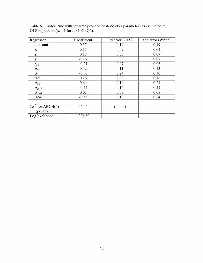
spectively. Table 6 then re-estimates the relation, allowing for separate coefficients since

18

1979:Q3, when Paul Volcker became Chair of the Federal Reserve. The OLS results repro-

duce the findings of the many researchers noted above that monetary policy seems to have

responded much more vigorously to disturbances since 1979, with the inflation coefficient γ1

increasing by 0.26 and the output coefficient γ2 increasing by 0.64.

However, the White standard errors for the coefficients on dtπt and dtyt are almost twice

as large as the OLS standard errors, and suggest that the increased response to inflation is

in fact not statistically significant and the increased response to output is measured very

imprecisely. Moreover, Engle’s LM test for the null of Gaussian errors with no heteroskedas-

ticity against the alternative of 4th-order ARCH leads to overwhelming rejection of the null

hypothesis.2 All of which suggests that, if we are indeed interested in measuring the

magnitudes by which these coefficients have changed, it is preferable to adjust not just the

standard errors but the parameter estimates themselves in light of the dramatic ARCH

displayed in the data.

I therefore estimated the following GARCH-t generalization of (18):

yt = x0tβ + vt

vt =phtεt

ht = κ+ ht

ht = α(v2t−1 − κ) + δht−1 (19)

with εt a Student’s t random variable with ν degrees of freedom. Iteration on (19) is

2 Siklos and Wohar (2005) also make this point.

19

initialized with h1 = 0. The log likelihood is then evaluated exactly as in (17). Maximum

likelihood estimates are reported in Table 7.

Once again generalizing a homoskedastic Gaussian specification is overwhelmingly fa-

vored by the data, with a comparison of the specifications in Tables 6 and 7 producing a

likelihood ratio χ(4) statistic of 183.34. The degrees of freedom for the Student’s t distrib-

ution are only 2.29, and the implied GARCH process is highly persistent (α+ δ = 0.82). Of

particular interest is the fact that the changes in the Fed’s response to inflation and output

are now considerably smaller than suggested by the OLS estimates. The change in γ1 is now

estimated to be only 0.09 and the change in γ2 has dropped to 0.05 and no longer appears

to be statistically significant.

Figure 5 offers some insight into what produces these results. The top panel illustrates

the tendency for interest rates to exhibit much more volatility at some times than others, with

the 1979:Q2 to 1982:Q3 episode particularly dramatic. The bottom panel plots observations

on the pairs (yt,∆rt) in the second half of the sample. The apparent positive slope in that

scatter plot is strongly influenced by the observations in the 1979-82 period. If one allowed

the possibility of serial dependence in the squared residuals, one would give less weight to

the 1979-82 observations, resulting in a flatter slope estimate over 1979-2007 relative to OLS.

This is not to attempt to overturn the conclusion of earlier researchers that there has

been a change in Fed policy in the direction of a more active policy. A comparison of the

changing-parameter specification of Table 7 with a fixed-parameter GARCH specification

produces a χ(4) likelihood ratio statistic of 18.22, which is statistically significant with a

20

p-value of 0.001. Nevertheless, the magnitude of this change appears to be substantially

smaller than one would infer on the basis of OLS estimates of the parameters.

Nor is this discussion meant to displace the large and thoughtful literature on possible

changes in the Taylor Rule, which has raised a number of other substantive issues not

explored here. These include whether one wants to use real-time or subsequent revised data

(Orphanides (2001)), the distinction between the “backward-looking” Taylor Rule explored

here and “forward-looking” specifications (Clarida, Galí, and Gertler, 2000), and continuous

evolution of parameters rather than a sudden break (Jalil, 2004; Boivin, 2006). The simple

exercise undertaken nevertheless does in my mind establish the potential importance for

macroeconomists to check for the presence of ARCH even when their primary interest is in

the conditional mean.

5 Conclusions.

The reader may note that both of the examples I have used to illustrate the potential

relevance of McARCH use the fed funds rate as the dependent variable. This is not entirely

an accident. Although Kilian and Gonçalves (2004) concluded that most macro series

exhibit some ARCH, the fed funds rate may be the macro series for which one is most likely

to observe wild outliers and persistent volatility clustering, regardless of the data frequency

or subsample. It is nevertheless, as the examples used here illustrate, a series that features

very importantly for some of the most fundamental questions in macroeconomics.

The rather dramatic way in which accounting for outliers and ARCH can change one’s

21

inference that was seen in these examples presumably would not be repeated for every

macroeconomic relation estimated. However, routinely checking something like a TR2

statistic, or the difference between OLS andWhite standard errors, seems a relatively costless

and potentially quite beneficial habit. And the assumption by many practitioners that we

can avoid all these problems simply by always relying on the White standard errors may not

represent best possible practice.

22

References

Baillie, Richard T., Tim Bollerslev, and Hans O. Mikkelsen. 1996. “Fractionally Inte-

grated Generalized Autoregressive Conditional Heteroskedasticity” Journal of Econometrics

74, pp.3-30.

Bera, Anil K., Matthew L. Higgins, and Sangkyu Lee. 1992. “Interaction between Auto-

correlation and Conditional Heteroscedasticity: A Random-Coefficient Approach,” Journal

of Business and Economic Statistics 10, pp. 133-142.

Boivin, Jean. 2006. “Has U.S. Monetary Policy Changed? Evidence from Drifting

Coefficients and Real-Time Data,” Journal of Money, Credit and Banking 38, pp. 1149-

1173.

_____, and Marc P. Giannoni. 2006. “Has Monetary Policy Become More Effective?”

Review of Economics and Statistics 88, pp. 445-462.

Bollerslev, Tim. 1986. “Generalized Autoregressive Conditional Heteroskedasticity,”

Journal of Econometrics 31, pp. 307—327.

_____. 1987. “A Conditionally Heteroskedastic Time Series Model for Speculative

Prices and Rates of Return,” Review of Economics and Statistics 69, pp.542-547.

_____. 2008. “Glossary to ARCH (GARCH),” in Festschrift in Honor of Robert F.

Engle, edited by Tim Bollerslev, Jeffry R. Russell and Mark Watson.

_____, Ray Y. Chou, and Kenneth F. Kroner. 1992. “ARCH Modeling in Finance,”

Journal of Econometrics 52, pp. 5-59.

_____, and Robert F. Engle. 1986. “Modeling the Persistence of Conditional Vari-

23

ances,” Econometric Reviews 5, pp. 1-50.

_____, and Hans Ole Mikkelsen. 1996. “Modeling and Pricing Long Memory in Stock

Market Volatility,” Journal of Econometrics 73, pp. 151-184.

_____, _____, and Jeffrey M. Wooldridge. 1988. “A Capital Asset Pricing Model

with Time-Varying Covariances”, Journal of Political Economy 96, pp. 116 - 131.

Box, George E. P., and Gwilym M. Jenkins. 1976. Time Series Analysis: Forecasting

and Control. Revised edition. San Francisco: Holden-Day.

Clarida, Richard, Jordi Galí, and Mark Gertler. 2000. “Monetary Policy Rules and

Macroeconomic Stability: Evidence and Some Theory,” Quarterly Journal of Economics

115, pp. 147-180.

Diebold, Francis X. 1988. Empirical Modeling of Exchange Rate Dynamics. New York:

Springer-Verlag.

Ding, Zhuanxin, Robert F. Engle, and Clive W.J. Granger. 1993. “A Long Memory

Property of Stock Market Returns and a New Model,” Journal of Empirical Finance 1, pp.

83-106.

Elder, John, and Apostolos Serletis. 2006. “Oil Price Uncertainty.” Working paper,

North Dakota State University.

Engle, Robert F. 1982(a). “Autoregressive Conditional Heteroskedasticity With Esti-

mates of the Variance of U.K. Inflation,” Econometrica 50, pp. 987-1008.

_____. 1982(b). “A General Approach to Lagrange Multiplier Model Diagnostics,”

Journal of Econometrics 20, pp. 83-104.

24

_____, and Gloria González-Rivera. 1991. “Semi-Parametric ARCHModels,” Journal

of Business and Economic Statistics 9, pp. 345-359.

_____, David Lilien and Russell Robins. 1987. “Estimation of Time Varying Risk

Premia in the Term Structure: the ARCH-M Model,” Econometrica 55, pp. 391-407.

_____, and Simone Manganelli. 2004. “CAViaR: Conditional Autoregressive Value at

Risk by Regression Quantiles,” Journal of Business and Economic Statistics 22, pp. 367-381.

_____, and Victor Ng. 1993. “Measuring and Testing the Impact of News On Volatil-

ity,” Journal of Finance 48, pp. 1749-1778.

Fountas, Stilianos and Menelaos Karanasos. 2007. “Inflation, Output Growth, and

Nominal and Real Uncertainty: Empirical Evidence for the G7,” Journal of International

Money and Finance 26: pp. 229-250.

Friedman, Benjamin M., David I. Laibson, and Hyman P. Minsky. 1989. “Economic

Implications of Extraordinary Movements in Stock Prices,” Brookings Papers on Economic

Activity 1989:2, pp. 137-189.

Gourieroux, Christian, and Alain Monfort. 1992. “Qualitative Threshold ARCH Mod-

els,” Journal of Econometrics 52, pp. 159-199.

Glosten, L. R., R. Jagannathan, and D.E. Runkle. 1993. “On the Relation between the

Expected Value and the Volatility of the Nominal Excess Return on Stocks,” Journal of

Finance 48, pp. 1779—1801.

Grier, Kevin B., and Mark J. Perry. 2000. “The Effects of Real and Nominal Uncer-

tainty on Inflation and Output Growth: Some GARCH-M Evidence,” Journal of Applied

25

Econometrics 15, pp. 45-58.

Hamilton, James D. 1994. Time Series Analysis. Princeton: Princeton University Press.

_____. Forthcoming. “Daily Changes in Fed Funds Futures Prices,” Journal of

Money, Credit and Banking.

_____. 2008. “Daily Monetary Policy Shocks and the Delayed Response of New Home

Sales,” Working paper, UCSD.

_____, and Raul Susmel. 1994. “Autoregressive Conditional Heteroskedasticity and

Changes in Regime,” Journal of Econometrics 64, pp. 307-333.

Harvey, Andrew, Esther Ruiz, and Enrique Sentana. 1992. “Unobserved Component

Time Series Models with ARCH Disturbances,” Journal of Econometrics 52: 129-157.

Higgins M.L., and A.K. Bera. 1992. “A Class of Nonlinear Arch Models,” International,

Economic Review 33, pp. 137—158.

Hentschel, L. 1995. “All in the Family: Nesting Symmetric and Asymmetric GARCH

Models,” Journal of Financial Economics 39, pp. 71-104.

Jalil, Munir. 2004. Essays on the Effect of Information on Monetary Policy, unpublished

Ph.D. dissertation, UCSD.

Judd, John P., and Glenn D. Rudebusch. 1998. “Taylor’s Rule and the Fed: 1970-1997,”

Federal Reserve Bank of San Francisco Review 3, pp. 3-16.

Kilian, Lutz, and Sílvia Gonçalves. 2004. “Bootstrapping Autoregressions with Condi-

tional Heteroskedasticity of Unknown Form,” Journal of Econometrics 123, pp. 89-120.

Lee, Kiseok, Shawn Ni, and Ronald A. Ratti. 1995. “Oil Shocks and the Macroeconomy:

26

The Role of Price Variability,” Energy Journal, 16, pp. 39-56.

Lee, Sang-Won, and Bruce E. Hansen. 1994. “Asymptotic Theory for the Garch (1,1)

Quasi-Maximum Likelihood Estimator,” Econometric Theory 10, pp. 29-52.

Lumsdaine, Robin L. 1996. “Consistency and Asymptotic Normality of the Quasi-

Maximum Likelihood Estimator in IGARCH(1,1) and Covariance Stationary GARCH(1,1)

Models,” Econometrica 64, pp. 575-596.

Milhøj,Anders. 1985. “The Moment Structure of ARCH Processes,” Scandinavian Jour-

nal of Statistics 12, pp. 281-292.

Milhøj, Aers. 1987. “A Conditional Variance Model for Daily Observations of an Ex-

change Rate,” Journal of Business and Economic Statistics 5, pp. 99-103.

Nelson Daniel B. 1991. “Conditional Heteroscedasticity in Asset Returns: A New Ap-

proach,” Econometrica 59, pp. 347—370.

Newey, Whitney K., and Kenneth D. West. 1987. “A Simple Positive Semi-Definite,

Heteroskedasticity and Autocorrelation Consistent Covariance Matrix,” Econometrica 55,

pp. 703-708.

Orphanides, Athanasios. 2001. “Monetary Policy Rules Based on Real-Time Data.”

American Economic Review 91. [[/ 964-985.

Pelloni, Gianluigi and Wolfgang Polasek. 2003. “Macroeconomic Effects of Sectoral

Shocks in Germany, the U.K. and the U.S.: A VAR-GARCH-M Approach,” Computational

Economics 21, pp. 65-85.

Piazzesi, Monika, and Eric Swanson. Forthcoming. “Futures Prices as Risk-Adjusted

27

Forecasts of Monetary Policy.” Journal of Monetary Economics.

Sack, Brian. (2004) “Extracting the Expected Path of Monetary Policy from Futures

Rates.” Journal of Futures Markets, 24, 733-754.

Sentana, Enrique. 1995. “Quadratic ARCH Models,” Review of Economic Studies 62,

pp. 639-661.

Servén, Luis. 2003. “Real-Exchange-Rate Uncertainty and Private Investment in LDCS,”

Review of Economics and Statistics 85, pp. 212-218.

Shields, Kalvinder, Nilss Olekalns, Ólan T. Henry, and Chris Brooks. 2005. “Measuring

the Response of Macroeconomic Uncertainty to Shocks,” Review of Economics and Statistics

87, pp. 362-370.

Siklos, Pierre L., and Mark E. Wohar. 2005. “Estimating Taylor-Type Rules: An Un-

balanced Regression?”, in Advances in Econometrics, vol. 20, edited by Thomas B. Fomby

and Dek Terrell. Amsterdam: Elsevier.

Stambaugh, Robert F. 1993. “Estimating Conditional Expectations when Volatility Fluc-

tuates,” NBER Working Paper 140.

Taylor, John B. 1993. “Discretion Versus Policy Rules in Practice,” Carnegie-Rochester

Conference Series on Public Policy 39, pp. 195-214.

White, Halbert. 1980. “A Heteroskedasticity-Consistent Covariance Matrix Estimator

and a Direct Test for Heteroskedasticity,” Econometrica 48, pp. 817-38.

Zakoian, J. M. 1994. “Threshold Heteroskedastic Models,” Journal of Economic Dynam-

ics and Control 18, pp. 931—955.

28

29

Table 1. How many ways can you spell “ARCH”? (A partial lexicography). ________________________________________________________________________ AARCH Augmented ARCH Bera, Higgins and Lee (1992) APARCH Asymmetric power ARCH Ding, Engle, and Granger (1993) ARCH-M ARCH in mean Engle, Lilien and Robins (1987) FIGARCH Fractionally integrated GARCH Baillie, Bollerslev, Mikkelsen (1996) GARCH Generalized ARCH Bollerslev (1986) GARCH-t Student’s t GARCH Bollerslev (1987) GJR-ARCH Glosten-Jagannathan-Runkle ARCH Glosten, Jagannathan, and Runkle (1993) EGARCH Exponential generalized ARCH Nelson (1991) HGARCH Hentschel GARCH Hentschel (1995) IGARCH Integrated GARCH Bollerslev and Engle (1986) MARCH Modified ARCH Friedman, Laibson, and Minsky (1989) MARCH Multiplicative ARCH Milhøj (1987) NARCH Nonlinear ARCH Higgins and Bera (1992) PNP-ARCH Partially Non-parametric ARCH Engle and Ng (1993) QARCH Quadratic ARCH Sentana (1995) QTARCH Qualitative Threshold ARCH Gourieroux and Monfort (1992) SPARCH Semiparametric ARCH Engle and Gonzalez-Rivera (1991) STARCH Structural ARCH Harvey, Ruiz, and Sentana (1992) SWARCH Switching ARCH Hamilton and Susmel (1994) TARCH Threshold ARCH Zakoian (1994) VGARCH Vector GARCH Bollerslev, Engle, and Wooldrige (1988)

30

Table 2. Fraction of samples for which indicated hypothesis is rejected by test of nominal size 0.05. -----------------------------------------------------------------------------------------------------

Errors Normally distributed

H0 Test based on T = 100 T = 200 T = 1000 ------------------- --------------------- --------- --------- ----------- β1 =0 (H0 is true) OLS standard error 0.152 0.200 0.327 β1 =0 (H0 is true) White standard error 0.072 0.063 0.054 β1 =0 (H0 is true) Newey-West standard error 0.119 0.092 0.062 εt homoskedastic (H0 is false) White TR2 0.570 0.874 1.000 εt homoskedastic (H0 is false) Engle TR2 0.692 0.958 1.000

Errors Student’s t with 5 degrees of freedom

H0 Test based on T = 100 T = 200 T = 1000 ------------------- --------------------- --------- --------- ----------- β1 =0 (H0 is true) OLS standard error 0.174 0.229 0.389 β1 =0 (H0 is true) White standard error 0.081 0.070 0.065 β1 =0 (H0 is true) Newey-West standard error 0.137 0.106 0.079 εt homoskedastic (H0 is false) White TR2 0.427 0.691 0.991 εt homoskedastic (H0 is false) Engle TR2 0.536 0.822 0.998

31

Table 3. OLS estimates of bias in monthly fed funds futures forecast errors. --------------------------------------------------------------------------- dependent estimated standard OLS ARCH(4) Log like- variable )( )( j

tu mean )ˆ( )( jµ error p-value LM p-value lihood ----------- ----------- --------- ------- ----------- -------- j = 1 month -2.66 0.75 0.001 0.006 -812.61 j = 2 months -3.17 1.06 0.003 0.204 -884.70 j = 3 months -3.74 1.27 0.003 0.001 -922.80

32

Table 4. Maximum likelihood estimates (asymptotic standard errors in parentheses) for EGARCH model of fed funds futures forecast errors. ------------------------------------------------------------------------------------------------------- horizon (j) )1(

tu )2(tu )3(

tu mean (µ) 0.12 0.43 0.27 (0.24) (0.34) (0.67) log average 5.73 6.47 7.01 variance (γ1) (0.42) (0.51) (0.54) trend in -22.7 -23.6 -17.1 variance (γ2) (3.1) (3.3) (3.8) | ut-1| (α) 0.18 0.15 0.30 (0.07) (0.07) (0.12) log ht-1 (δ) 0.63 0.74 0.84 (0.16) (0.22) (0.11) Student t 2.1 2.2 4.1 degrees of (0.4) (0.4) (1.2) freedom (υ) log likelihood -731.08 -793.38 -860.16

33

Table 5. Fixed-coefficient Taylor Rule as estimated from full sample OLS regression. Regressor Coefficient Std error (OLS) Std error (White) constant 0.06 0.13 0.18 πt 0.13 0.04 0.06 yt 0.37 0.07 0.11 yt-1 -0.27 0.07 0.10 rt-1 -0.08 0.03 0.03 ∆rt-1 0.14 0.07 0.15 TR2 for ARCH(4) (p-value)

23.94 (0.000)

Log likelihood -252.26

34

Table 6. Taylor Rule with separate pre- and post-Volcker parameters as estimated by OLS regression (dt = 1 for t > 1979:Q2). Regressor Coefficient Std error (OLS) Std error (White) constant 0.37 0.19 0.19 πt 0.17 0.07 0.04 yt 0.18 0.08 0.07 yt-1 -0.07 0.08 0.07 rt-1 -0.21 0.07 0.06 ∆rt-1 0.42 0.11 0.13 dt -0.50 0.24 0.30 dtπt 0.26 0.09 0.16 dtyt 0.64 0.14 0.24 dtyt-1 -0.55 0.14 0.21 dtrt-1 0.05 0.08 0.08 dt∆rt-1 -0.53 0.13 0.24 TR2 for ARCH(4) (p-value)

45.45 (0.000)

Log likelihood -226.80

35

Table 7. Taylor Rule with separate pre- and post-Volcker parameters as estimated by GARCH-t maximum likelihood (dt = 1 for t > 1979:Q2). Regressor Coefficient Asymptotic std error constant 0.13 0.08 πt 0.06 0.03 yt 0.14 0.03 yt-1 -0.12 0.03 rt-1 -0.07 0.03 ∆rt-1 0.47 0.09 dt -0.03 0.12 dtπt 0.09 0.04 dtyt 0.05 0.07 dtyt-1 0.02 0.07 dtrt-1 -0.01 0.03 dt∆rt-1 -0.01 0.11 GARCH parameters constant 0.015 0.010 α 0.11 0.05 δ 0.71 0.07 ν 2.29 0.48 Log likelihood -135.13

36

Figure 1. Asymptotic rejection probability for OLS t-test that autoregressive coefficient is zero as a function of GARCH(1,1) parameters α and δ. Note: null hypothesis is actually true and test has nominal size of 5%.

37

Figure 2. Fraction of samples in which OLS t-test leads to rejection of the null hypothesis that autoregressive coefficient is zero as a function of the sample size for regression with Gaussian errors (solid line) and Student’s t errors (dashed line). Note: null hypothesis is actually true and test has nominal size of 5%.

102 103 104 1050

0.1

0.2

0.3

0.4

0.5

0.6

0.7

0.8

0.9

1

Sample size (T)

NormalStudent t

38

Figure 3. Average value of T times estimated standard error of estimated autoregressive coefficient as a function of the sample size for White standard error (solid line) and OLS standard error (dashed line).

102 103 104 1050

1

2

3

4

5

6

Sample size (T)

WhiteOLS

39

Figure 4. Plots of 1-month-ahead forecast errors )( )( jtu as a function of month t based on j

= 1-, 2-, or 3-month ahead futures contracts.

1 month

1988 1989 1990 1991 1992 1993 1994 1995 1996 1997 1998 1999 2000 2001 2002 2003 2004 2005 2006-60-50-40-30-20-10

0102030

2 month

1988 1989 1990 1991 1992 1993 1994 1995 1996 1997 1998 1999 2000 2001 2002 2003 2004 2005 2006-75

-50

-25

0

25

50

75

3 month

1988 1989 1990 1991 1992 1993 1994 1995 1996 1997 1998 1999 2000 2001 2002 2003 2004 2005 2006-80

-60-40

-20

020

4060

80

40

Figure 5. Change in fed funds rate for the full sample (1956:Q2-2007:Q1), and scatter plot for later subsample (1979:Q2-2007:Q1) of change in fed funds rate against deviation of GDP from potential.

Change in fed funds rate, 1956:Q2-2007:Q1

date

chan

ge

in f

un

ds

rate

1956 1959 1962 1965 1968 1971 1974 1977 1980 1983 1986 1989 1992 1995 1998 2001 2004 2007-4

-2

0

2

4

6

8

Scatter diagram, 1979:Q2-2007:Q1

GDP deviation

chan

ge

in f

un

ds

rate

-8 -6 -4 -2 0 2 4

-4

-2

0

2

4

6

8