macroeconomics 1 (econ1102)

Macroeconomics 1

(ECON1102)

Cameron Gordon

2nd Semester 2019

“The AD-AS Model”

• We have considered a long-run model of the

macroeconomy, namely the Solow-Swan growth model.

Now we must build a comparable model for the macro-

economy in the short-run.

• The Aggregate Demand and Aggregate Supply (AD-AS)

model examines how short-run fluctuations in real GDP

and the price level occur and how they affect total output.

• The basic idea: Real GDP and the price level are

determined in the short run by the intersection of the short-

run Aggregate Demand (AD) curve and the short-run

Aggregate Supply (AS) curves.

AD-AS

2

Aggregate demand (AD) curve: A curve that shows the

relationship between the price level (or inflation rate as an

alternative but equivalent specification) and the quantity of

real GDP demanded by households, firms and the

government, i.e. the whole economy. We derived this curve

last time from the AE model.

Aggregate supply (AS) curve: In this case we have two

versions: Short-run aggregate supply (SRAS) curve: A

curve that shows the relationship in the short run between

the price level and the quantity of real GDP supplied; Long-

run aggregate supply (LRAS) curve: a similar curve for the

long-run. Unless explicitly noted reference to an AS curve

can be assumed to be short-run.3

AD and AS curves

4

The AD Curve v market demand curves

• Remember that the AD curve is fundamentally different than the

microeconomic market demand curve.

• An AD curve is built up from the demand expenditures side of

the whole economy – C+I+G+NX – and in this sense

represents a short-run balance across these components

across all micro-markets for goods and services. It shows total

AD (or AE) associated with different price levels.

• A market demand curve is, by contrast, the sum of willingness-

to-pay for a given good at various prices across all potential

buyers of that good. Both D curves slope downward but the

reason for a negatively sloped market demand curve is due to

the fact consumers are generally willing to buy less of a good

the more its price increases. (The AS curve is also different

from the market S curve – more on that later).

Violating the classical dichotomy• Note that positing a relationship between nominal

price levels and real output violates the classical dichotomy and the neutrality of money.

• This is because the dichotomy/neutrality holds only in the long-run.

• AD is a short-run model where lags and rigidities in adjustment lead to nominal quantities having real effects.

• The same can be said for the AS curve and its interactions with AD. This is a short-run model and in the short-run nominal quantities can affect real ones.

5

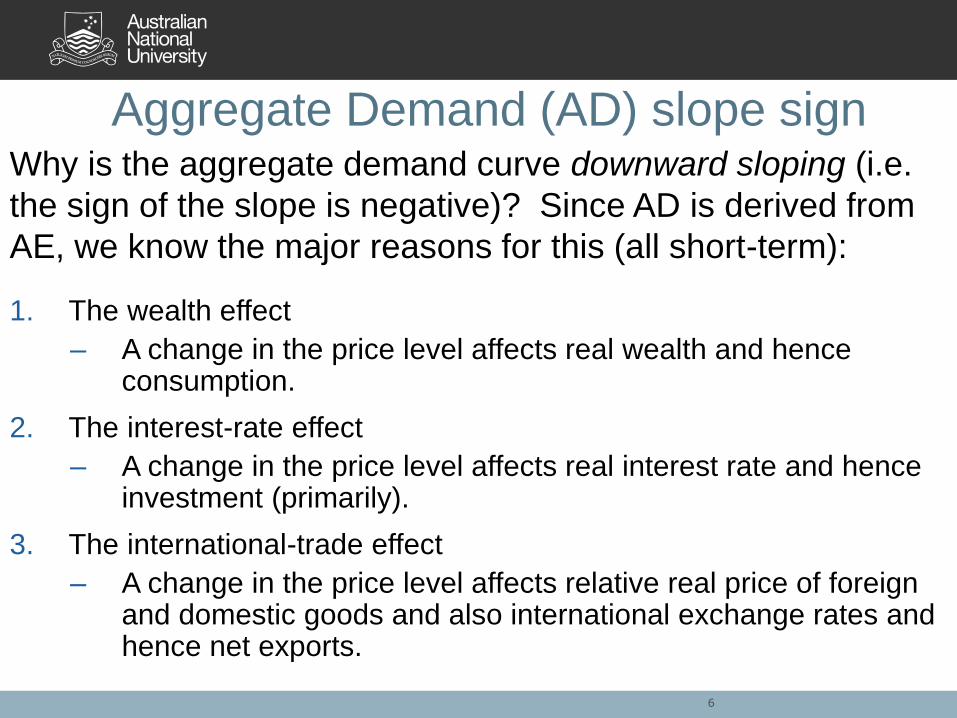
Why is the aggregate demand curve downward sloping (i.e.

the sign of the slope is negative)? Since AD is derived from

AE, we know the major reasons for this (all short-term):

1. The wealth effect

– A change in the price level affects real wealth and hence consumption.

2. The interest-rate effect

– A change in the price level affects real interest rate and hence investment (primarily).

3. The international-trade effect

– A change in the price level affects relative real price of foreign and domestic goods and also international exchange rates and hence net exports.

6

Aggregate Demand (AD) slope sign

• The AD curve shows the relationship between the price level

and the quantity of real GDP demanded, holding everything

else constant. Since relationships of C, I, G and NX to AD

given changes in price level are all inverse, price level rises

reduce one or more of these components, reduce real GDP

and make the sign of the AD slope negative.

• The strength of the various effects makes the curve shallower

or steeper, ceteris paribus (i.e. changes the magnitude of the

slope). Thus, if I, say, is very sensitive to real interest rate

changes as affected by price level, then the AD curve will be

flatter than when I is not very sensitive to such changes.

7

Aggregate Demand (AD) slope magnitude

• Here is an example of two

different AD curves. AD1 is

flatter than AD2, which means

that the ‘elasticity’

(responsiveness) of Real

GDP to price level is much

greater than that of the

steeper AD2.

• So we can see that a change

in the price level in either

direction changes Real GDP

much more where AD1 holds

than for AD2 (which is

relatively ‘inelastic’).

8

Price level

Real GDP

AD1

AD2

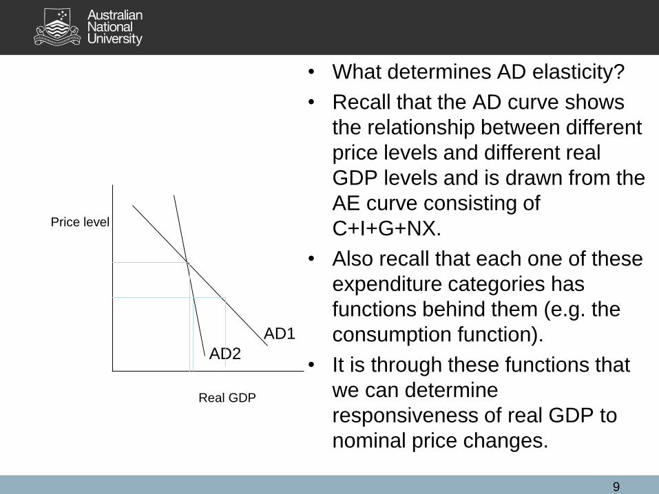
• What determines AD elasticity?

• Recall that the AD curve shows

the relationship between different

price levels and different real

GDP levels and is drawn from the

AE curve consisting of

C+I+G+NX.

• Also recall that each one of these

expenditure categories has

functions behind them (e.g. the

consumption function).

• It is through these functions that

we can determine

responsiveness of real GDP to

nominal price changes.

9

Price level

Real GDP

AD1

AD2

A conceptual example• Suppose we have two different economies (or the

same economy but in two different years). Call them Economy 1 and Economy 2. (If we were looking at the same economy but at different times we could say Economy 1t and Economy 1t+5 to indicate, for example, time t and then time t+5, e.g. 5 years later for Economy 1)

• Both economies have the same expenditure functions except that 1 has an investment function (I) where investors are much more responsive to changes in short-run real interest rates than with 2.

• Which economy has a flatter AD curve?

10

Answer• First we have to think of what ‘flatter’ means. It means

that a change in the price level will yield a greater change in Real GDP, ceteris paribus. In other words, a flatter curve will be more ‘elastic’ or responsive.

• Conceptually it should then be clear that 1 will have a flatter (more responsive) curve than 2 because the economies (Y=C+I+G+NX) are entirely identical except for their I functions, where I in economy 1 will adjust more to real interest rate changes than I in 2.

• Intuitively what is happening is that I in 1 will shift much more in response to a given a change in nominal interest rates in the short-run than in 2 as price level changes in 1 will, by changing the real interest rate, up or down, yield a greater change in I in that economy than in 1.

11

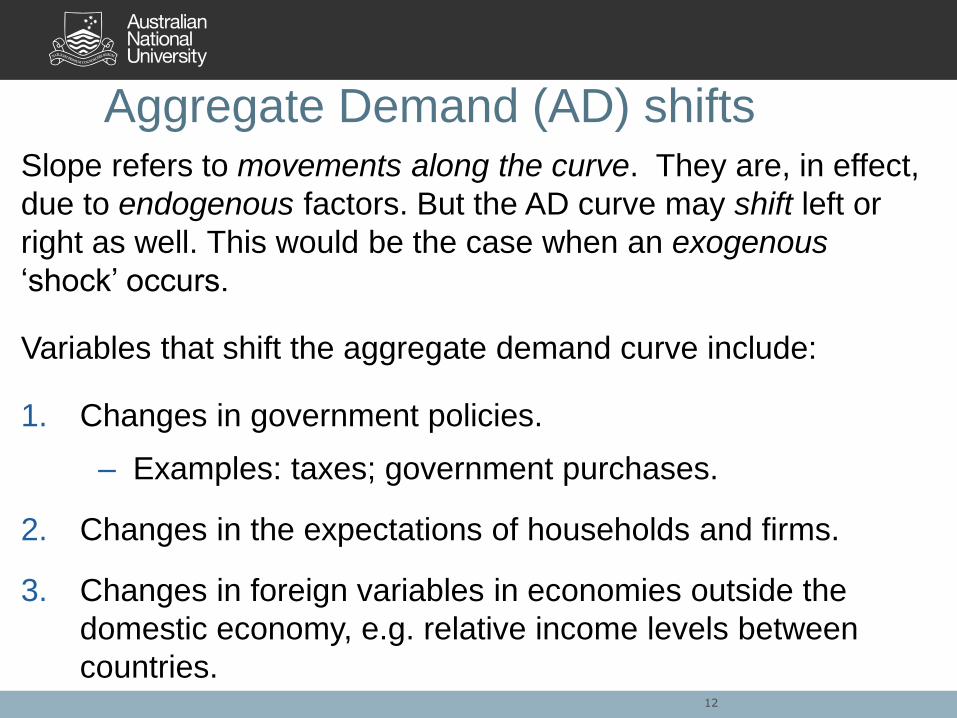
Slope refers to movements along the curve. They are, in effect,

due to endogenous factors. But the AD curve may shift left or

right as well. This would be the case when an exogenous

‘shock’ occurs.

Variables that shift the aggregate demand curve include:

1. Changes in government policies.

– Examples: taxes; government purchases.

2. Changes in the expectations of households and firms.

3. Changes in foreign variables in economies outside the

domestic economy, e.g. relative income levels between

countries.12

Aggregate Demand (AD) shifts

A note on ‘shifts’ versus ‘movements along’• In a movement along a curve everything is held constant

and we are looking at a line that shows the tradeoff between real GDP and different possible price levels, driven by the components of AE, ceteris paribus.

• In shifts of the curve there is an exogenous shock that changes the overall economic structure and the associated functions, e.g. an increase in government taxes and how that shifts C, G, I and NX entirely, upsetting former patterns.

• Thus if price level changes but nothing else does, we have a movement along the AD curve: i.e. everything else in the economy, including the functions behind C, I, G and NX, are fixed and we are just looking at the set tradeoff between total real GDP and changes in price levels. If there as a change to the parameters, e.g. expectations about consumer incomes, then this shifts AD.

13

14

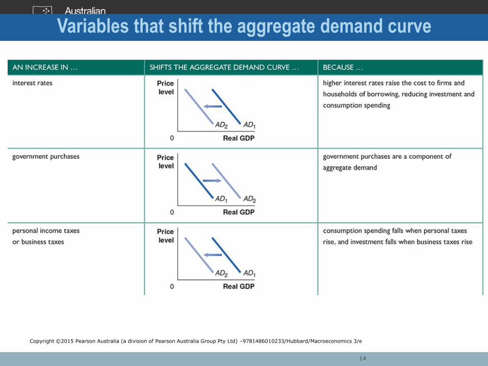
Variables that shift the aggregate demand curve

Copyright ©2015 Pearson Australia (a division of Pearson Australia Group Pty Ltd) –9781486010233/Hubbard/Macroeconomics 3/e

Variables that shift the aggregate demand curve

15 Copyright ©2015 Pearson Australia (a division of Pearson Australia Group Pty Ltd) –9781486010233/Hubbard/Macroeconomics 3/e

15

Prior example of Economies 1 and 2• One might now ask: a change in price

level can affect real interest rates which

affects real GDP and this was a

movement along the AD curve. But isn’t

that also a shift of the curve?

• The answer is: it depends on what you

are talking about exactly. The AD curve

shows a static tradeoff between price

level and AE (C+I+G+NX), that tradeoff

being determined by channels such as

the interest rate, ceteris paribus, at that

moment at existing spending functions.

• But if the whole structure of interest rates

changes because of, say, a change in

central bank policy, then we have

changed the whole economy and shifted

the whole set of tradeoff patterns as a

result. This is a shift of the whole curve,

not just a movement along it.

• In our prior example, we had two

economies with everything the

same, including the interest rate

structure (often referred to as the

term structure of interest rates) but

one economy had a different I

function than the other and hence a

different shaped AD curve (read:

static set of tradeoffs between real

GDP and price level).

• If we now introduced an identical

exogenous shock to those

economies in the form of a tighter

central bank monetary policy (i.e.

term structure of interest rates goes

up) both curves would shift – but

they would also both keep their

relative slopes (ceteris paribus).

16

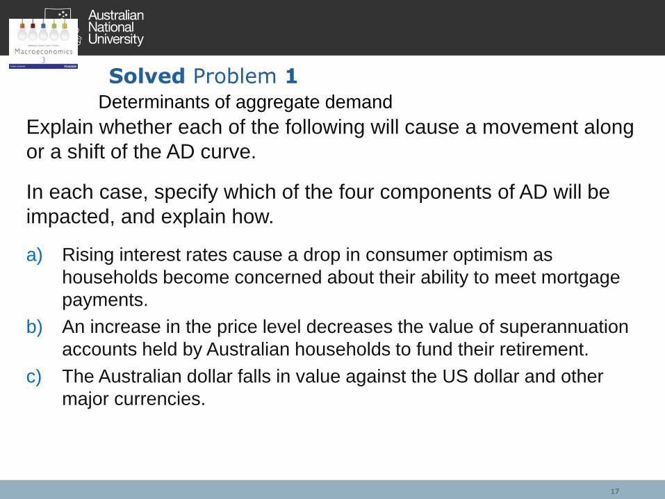
Explain whether each of the following will cause a movement along

or a shift of the AD curve.

In each case, specify which of the four components of AD will be

impacted, and explain how.

a) Rising interest rates cause a drop in consumer optimism as

households become concerned about their ability to meet mortgage

payments.

b) An increase in the price level decreases the value of superannuation

accounts held by Australian households to fund their retirement.

c) The Australian dollar falls in value against the US dollar and other

major currencies.

Solved Problem 1Determinants of aggregate demand

17

(a): Households become pessimistic about the future. In order to

ensure they can continue to meet higher mortgage payments caused

by rising interest rates, consumers spend less in the present. The AD

curve will shift inwards to the left.

(b): This is an example of the wealth effect. An increase in the price

level decreases the real value of superannuation funds. Aggregate

quantity demanded will decrease as households spend less in order to

contribute more to their superannuation. This is reflected in an upward

movement along the AD curve.

(c): A fall in the value of the Australian dollar means it costs less in

terms of other currencies to buy Australian dollars, and hence also

goods, services and investments denominated in Australian dollars. Net

exports should therefore increase, and this will be reflected in an

increase in aggregate demand—a shift to the right of the AD curve.

18

Solved Problem 1

Aggregate Supply (AS)

• Now we must talk about Aggregate Supply in the short-run macroeconomy.

• We have two AS curves one for the long-run (LRAS – Long Run Aggregate Supply) and one for the short-run (SRAS – Short Run Aggregate Supply).

• Let’s take a closer look at these two.

• (Note: if ‘AS’ – Aggregate Supply – is referred to one can assume that it is being used synonymously with SRAS.

19

Long-run aggregate supply (LRAS) curve: A curve that

shows the relationship in the long run between the price level

and the quantity of real GDP supplied. The long-run

aggregate supply curve shows that, in the long run, increases

in the price level do not affect the level of real GDP. That is, in

the long-run the classical dichotomy holds and price

levels/inflation do NOT affect real GDP. The long-run

aggregate supply curve is a vertical line at potential GDP.

Conceptually one attains the potential GDP number from the

Solow-Swan long-run model (LRAS) and the goal of growth

policy is to increase that number. The goal of short-run policy

is to make sure the macroeconomy is hitting that number.

Aggregate Supply (AS) – (1) long run

20

Price level

Real GDP (billions of dollars)

0 $1100

100

LRASYear 1

$1140 $1170

95

112

LRASYear 2 LRASYear 3

The long-run aggregate supply curve

21

Shifts in the LRAS

Changes in the price level do not affect the level of aggregate

supply in the long run. Therefore, the long-run aggregate

supply (LRAS) curve is a vertical line at potential GDP. For

instance, the price level in the prior graph was 100 in Year 1

and potential GDP was $1100 billion. If the price level had

been 95, or if it had been 112, LRAS would still have been a

constant $1100 billion.

But the LRAS curve DOES move (shift) with time as the

number of workers in the economy increases, more

machinery and equipment is accumulated and technological

change occurs. In other words, The LRAS curve shifts

because potential GDP increases over time (assuming

positive growth). (Think: Solow-Swan growth model)22

• Short-run aggregate supply (SRAS) curve: an

upward sloping curve, showing the relationship in the

short-run between price level and real GDP supplied; in

the short run, firms will produce more in response to higher

prices. (Money is NOT neutral in the short run).

• Broadly speaking, this is because the prices of inputs (i.e. L

and K) tend to rise more slowly than the prices of final

products. Reasons for this include:

– Contracts that make some wages and prices ‘sticky’.

– Firms that are often slow to adjust wages.

– Menu costs – costs of adjusting prices - that make some prices sticky.

23

Aggregate supply (AS) – (2) Short run

SRAS upward slope in detail

• There are three major theories that potentially ‘explain’ the positive relationship between inflation (or price level) and output.

• These are not mutually exclusive and can be present at the same time, though some economists favour one over another.

• (1) money illusion

• (2) Sticky wages (‘Keynesian’)

• (3) Sticky prices (‘New Keynesian’)

24

1. Money Illusion• This refers to the idea that in the short-run people can ‘misread’ inflation

as higher or lower than it actually is. People plan for the future based on

their expectations of inflation when what counts in the end is actual

inflation. If actual inflation during a period is different than the inflation

they think has prevailed, they can have a (temporary) illusion as to the

real value of wages or prices or interest rates based on a (temporary)

misunderstanding of what inflation actually is.

• Thus a producer may first see rising nominal product prices as a real

price increase if there is mismatch between what they think inflation is

and what it actually is, and often this is what happens. E.g. a firm might

see the prices they get for their goods go up by 5%, think inflation is 2%

and conclude they have gained a 3% real price increase. This will

cause them to invest more – until they find out that actual inflation was

5%. But in the short-run inflation is tied to higher output.

• Keynes noted this phenomenon. New Classical theorists (e.g. Robert

Lucas) took this and made a whole theory based on this – more later.

25

2. Sticky wages• Wages may take more time to adjust than prices, based on things like

contracts (e.g. enterprise agreements for multiple years), and social

conventions such as perceptions of fairness, which are slow to

adjust.

• If actual inflation is below what it was expected to be when wages

were set then output will fall since the real wage is higher than

expected – until wages can finally adjust. The opposite is true for

when actual inflation is higher than it was expected to be when

wages were set. Firms now have lower real wages in actual fact,

they know it, and rationally increase output. Again, positive inflation is

associated, short-run, with higher output. This dynamic is often called

‘Keynesian’ because Keynes did consider this scenario at some

length. NOTE: This is an impact separate from ‘money illusion’

which refers to actions taken based on a misreading of reality. Here

there is a short-run real effect that is seen and ‘rationally’ reacted to.

26

3. Sticky prices• There also may be sticky prices for goods and services (as

opposed to prices of labour, i.e. wages). E.g. for some goods there may be long-term contracts with purchasers or complex pricing schemes that take time to be adjusted.

• In this case firms with sticky nominal prices have, until they can adjust them, real prices that are affected by actual inflation. If inflation is higher than expected, then these real prices are lower and this stimulates demand and output; if lower, the opposite. In both cases higher inflation is associated with higher output in the short-run.

• This is sometimes called ‘New Keynesian’, associated with theorists of that school and is distinguished from Keynes’ writings which focused on the age stickiness side (Keynes just did not consider price stickiness in any great detail).

27

The SRAS curve shows the short-run relationship between

the price level and the quantity of goods and services (real

GDP) firms are willing to supply, holding everything else

constant.

Changes in the price level are depicted as movements

along a stationary short-run aggregate supply curve.

But, just as with AD, SRAS can shift too, when there is

some kind of ‘exogenous’ shock, such as: expected

changes in the future price level; adjustments of workers

and firms to errors in past expectations about the price

level; unexpected changes in the price of an important

natural resource. 28

SRAS shifts v movements

Price level


0 $1000

100

SRASYear 1

SRASYear 2

103

1. If firms and workers expect the price level to be 3% higher in year 2

than in year 1 …

2. … the SRAS curve will shift to the left to reflect

worker and firm expectations of rising costs.

How expectations of the future price level affect short-run aggregate supply

29

Expectations of the future price level and SRAS

• What the graph is depicting is the following:

• The SRAS curve shifts to reflect workers’ and firms’ expectations of future prices.

• If workers and firms expect the price level to rise by 3% from 100 to 103, they will adjust their wages and prices by that amount.

• Holding constant all other variables that affect aggregate supply, the SRAS curve will shift to the left.

• If workers and firms expect the price level to be lower in the future, the SRAS curve will shift to the right.

30

Variables that shift both SRAS and LRAS

Some variables shift ONLY the SRAS, e.g. inflation expectations.

But some increase BOTH SRAS and LRAS at the same time.

Two key ones are:

• Increases in the labour force (L) and/or in the capital stock

and/or in resources (K).

• Technological change (A).

These changes have both short-run and long-run effects. The

Solow-Swan model indicates this (Y=f(K,L)). So changes in

these factors both change long-run growth and also the tradeoff

between price level and short-run output.

31

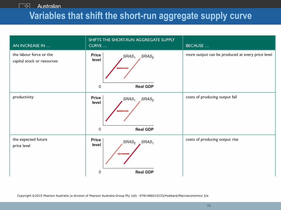
Variables that shift the short-run aggregate supply curve

32


33

Variables that shift the short-run aggregate supply curve


Shifts versus movements along redux• Remember the SRAS curve, like the AD curve, shows

the tradeoff between inflation and output in the short-run, ceteris paribus.

• As soon as we exogenously change something, such as the entire schedule of wages and prices across an economy, the curve will generally shift too – i.e. there is now a new tradeoff curve.

• The slope can change too, if there are changes in relationships, e.g. a change in technology can also change the relationship between output and a particular natural resource (e.g. oil) and make the SRAS curve more or less elastic with respect to inflation depending on how output’s relationship to that input is changed. (We’ll generally stick just to shifts however).

34

As with AD and market D, SRAS is different from a market S curve

• A market supply curve shows true marginal cost (MC) for producers in a particular market, assuming that input relative prices remain constant.

• As the price of good X rises, a seller is willing to supply more of good X given their MC, yielding an upward slope of the supply curve for good X. We can add up all sellers to get an aggregate market supply (S) curve) but whatever the scale changes in the price level have no effect on true MC and hence no effect on amount supplied at a given price.

• The SRAS curve shows how changes in the price level changes the amount producers in aggregate will offer to the whole economy in the short-run. In the short run, nominal changes can affect sales revenue and induce output changes.

35

• We now can define the equilibrium condition.

• In long-run equilibrium, the aggregate demand (AD) and short-

run aggregate supply (AS) curves intersect at a point along the

long-run aggregate supply (LRAS) curve.

• In the short-run, equilibrium is where the SRAS and the AD

curve intersect.

• In the long-run case, this equilibrium indicates that short-run

actual output is equal to long-run potential output and there is

‘full employment’ and no under- or over-utilized capacity.

• There may well be over- or under-capacity with the short-run

equilibrium.

Macroeconomic equilibrium in the long run and the short run

36

Price level

Real GDP (billions of dollars)0 $1000

100

Short-run aggregate supply

(SRAS)

Aggregate demand (AD)

Aggregate demand and aggregate supply

37

Price level

Real GDP (billions of

dollars)

0 $1000

100

SRAS

AD

LRAS

Long-run macroeconomic equilibrium

38

Interpretation• In long-run macroeconomic equilibrium, the AD and SRAS curves

intersect at a point on the LRAS curve. In our first figure,

equilibrium occurs at a real GDP of $1000 billion and a price level

of 100.

• For the second figure, in the short run, real GDP and the price

level are determined by the intersection of the AD curve and the

SRAS curve. In the figure, real GDP is measured on the

horizontal axis, and the price level is measured on the vertical

axis. In this example, equilibrium real GDP is still $1000 billion

and the equilibrium price level is still 100.

• Note that for the long-run the Classical Dichotomy holds in

equilibrium – the price level is irrelevant. It could 200, 1000 or 10.

• But in the short-run price level is important in determining real

GDP in the short-run.39

We can now use this model to analyze business cycles. The

following analysis of the aggregate demand and aggregate

supply model begins with a simplified case, using two

assumptions:

1. The economy has not been experiencing any inflation. The

price level is currently at 100, and workers and firms expect it

to remain at 100 in the future.

2. The economy is not experiencing any long-run economic

growth. Potential GDP is at $1000 billion and will remain at

that level in the future.

40

Macroeconomic equilibrium in the long run and the short run: business cycles

Recession

• Assume there is some decline in AD (e.g. I suddenly falls).

The short-run effect of a decline in aggregate demand will

yield:

– AD curve shifts left, and real GDP declines.

• Adjustment back to potential GDP in the long run.

– Automatic adjustment mechanism: SRAS curve shifts

right (which may take several years).

41

Price level

Real GDP (billions of dollars)0

1000

100

SRAS1

AD1

LRAS

AD2

A

B98

$980

SRAS2

C

1. A decline in investment shifts AD to the left causing a recession.

2. As firms and workers

adjust to the price level

being lower than expected,

costs will fall, and cause

SRAS to shift to the right.

3. Equilibrium moves from point B back to potential GDP at point C, with a lower price level.

96

The short-run and long-run effects of a decrease in aggregate demand

42


AS-AD dynamics of our recession graph• In the short run, a decrease in aggregate demand

causes a recession. In the long run it causes only a decrease in the price level.

• The decline in investment shifts aggregate demand from AD1 to AD2. Short-run equilibrium moves from potential GDP at point A to recession at point B.

• The price level of 98 at point B is lower than the price level of 100 that workers and firms had expected. As workers and firms adjust to the lower price level, prices and wages fall, and the SRAS curve shifts from SRAS1 to SRAS2.

• Equilibrium moves from point B back to potential GDP at point C, with a lower price level of 96.

• Note that the long-run structure of the economy is a re-equilibrating force for the short-run.

43

Expansion

• Now let’s look at the opposite scenario of the short-run

effect of an increase in aggregate demand.

– AD curve shifts right, and real GDP and the price

level rise.

• Adjustment back to potential GDP in the long run.

– Automatic adjustment mechanism: SRAS curve shifts

left (which may take a year or more).

44

Price level

0$1000

106

SRAS1

AD1

LRAS

AD2

C

B103

1030

SRAS2

A

1. An increase in investment shifts AD to the right, causing an inflationary expansion. 2. As firms and workers

adjust to the price level being higher than expected,

costs will rise, and cause SRAS to shift to the left.

3. Equilibrium moves from point B back to potential GDP at point C, with a higher price level.

100


The short-run and long-run effects of an increase in aggregate demand

45


AS-AD dynamics of our expansion graph• In the short run, an increase in aggregate demand

causes an increase in real GDP. In the long run it causes only an increase in the price level (same assumptions as before).

• The increase in investment shifts aggregate demand from AD1 to AD2. Short-run equilibrium moves from potential GDP at point A to beyond potential GDP at point B.

• The price level of 103 at point B is higher than the price level of 100 that workers and firms had expected. As workers and firms adjust to the higher price level, prices and wages rise, and the SRAS curve shifts from SRAS1 to SRAS2.

• Equilibrium moves from point B back to potential GDP at point C, with a higher price level of 106.

46

Supply shock

• A supply shock is an unexpected event that causes the

short-run aggregate supply curve to shift. If inward, it is a

negative shock; it outward, it is positive shock. The short-run

effect of a negative supply shock:

SRAS curve shifts left, real GDP falls and the price level

rises.

• Adjustment back to potential GDP in the long run:

SRAS curve shifts right (which may take several years).

• Stagflation, (a combination of inflation and recession),

usually results from a negative supply shock, at least

according to this model.

47

(b) Adjustment back to potential GDP –

the long-run effect of a supply shock.

0

(a) A recession with a rising price level – the

short-run effect of a supply shock.

SRAS1

AD

100

10000

1000$970

2. Equilibrium

moves from

point B to

potential GDP

at the original

price level.

1. An increase in oil

prices shifts SRAS

to the left …

Price

level

Real GDP

(billions of

dollars)

104

$970

LRAS SRAS2

A

B

AD

LRAS SRAS2

SRAS1

104

100

B

A

The short-run and long-run effects of a supply shock1. The recession caused by the

supply shock eventually leads to

falling wages and prices, shifting

SRAS back to its original position.

2. …moving short-run

equilibrium to point B, with

lower real GDP and a

higher price level.

Price

level

Real GDP

(billions of

dollars)

48


• Panel (a) shows that a supply shock, such as a large increase in oil prices, will cause a recession and a higher price level in the short run. The recession caused by the supply shock increases unemployment and reduces output.

• In panel (b), rising unemployment and falling output result in workers being willing to accept lower wages and firms being willing to accept lower prices. The SRAS curve shifts from SRAS2 to SRAS1.

• Equilibrium moves from point B back to potential GDP and the original price level at point A.

49

‘Stagflation’ • We will consider this in more detail later on in the course, but there was, for a couple of decades, a notion that one could not have rising inflation and rising unemployment at the same time –the definition of ‘stagflation’ (stagnation together with inflation).

• As our simple model shows, it is possible and the basic explanation for it is some sort of supply shock. This model can thus be applied to the stagflation that gripped much of the developed world in the 1970s.

• For example one can see weak to negative real GDP growth in the UK in the late 1960s and much of the 70s paired with very strong inflation. This shook up the world of macroeconomic thought and policy – as we will see next week.

50

The lighter side of stagflation

51

Using the model to explain inflation

more generally• The SRAS and AD curves have price levels

contained within them.

• AD-AS models can thus show two possible causes of inflation (increases in the rate of change of price levels) caused by shocks.

• (1) Cost-push inflation is what we have just illustrated: a rise in costs due to a supply shock and an inward shift of AS.

• (2) Demand-pull inflation is what we illustrated earlier with our expansion example: an increase in AD and an outward shift in AD.

52

Assume the economy is initially in equilibrium with long-run

aggregate supply constant.

Now suppose growing GDP in China and India leads to an increase

in demand and higher prices for Australian resources.

Explain both the initial change in equilibrium and the longer-term

effect.

Using the aggregate demand and aggregate supply model

Solved Problem 2

53

Solving the problem:

• An increase in demand for Australian exports will cause an

increase in aggregate demand represented by a rightward shift of

the AD curve. Short-run equilibrium will move beyond potential

GDP, causing an increase in the price level.

• The price level is now higher than workers and firms had

expected. As workers and firms adjust to the higher price level,

prices and wages rise, and the short-run aggregate supply curve

shifts inwards to the left.

• Equilibrium moves back to potential GDP, but at a higher price

level.

54

Solved Problem 2

Using the aggregate demand and aggregate supply model

Simplifying assumption: no feedback loops

• Our simple expositions thus far implicitly assume no long-run growth and no feedback loop between price level and the initial shift in the AD curve.

• With feedback loops, the transition dynamics (to use the technical term) would be complicated. For example, a first AD shift would affect inflation which would then shift AD again, leading to a series of ‘vibrations’ in the shifts. Introducing these makes for a more complex graph and adjustment process and will lead to a different calculated equilibrium real output/price level. The basic dynamics, though, would not change. Relaxing these assumptions allows for more precise predictions and robust simulations of real GDP and price level dynamics.

• Similarly, for long-term growth: the LRAS will also be shifting, making for more complexity but more realism.

55

So let’s relax these simplifying assumptions now to get a

dynamic aggregate demand and aggregate supply model.

Three changes to the basic model will now be made, relaxing

the assumptions we made earlier and now incorporating more

complex transition dynamics:

1. Potential GDP increases continually, shifting the LRAS

curve to the right.

2. During most years the AD curve shifts to the right.

3. Except during periods when workers and firms expect high

rates of inflation, the SRAS curve shifts to the right.

A dynamic AD-AS model

56

Price level

0 $1000

100

SRAS1

AD1

LRAS1

AD2

A

SRAS2

1. The economy begins in equilibrium at point A with SRAS1 and AD1 intersecting at a point on LRAS1.

5. The dynamic AD-AS model allows us to give a more accurate account of changes in real GDP and the price level.

1030

LRAS2

3. The same factors that cause the LRAS curve to shift during the year also cause the SRAS curve to shift.

4. During the course of the year, rising income and population, increasing investment, and increasing government purchases cause the AD curve to shift, and the economy ends in a new equilibrium at point B.

2. During the course of a year, increases in the labour force and capital stock as well as

technological change cause a shift from LRAS1 to LRAS2.


A dynamic aggregate demand and aggregate supply model

B

57

Price level

0 $1000

100

SRAS1

AD1

LRAS1

AD2

A

B

SRAS2

1. If AD shifts to

the right more

than LRAS …

2. …the price

level rises.

1050

LRAS2

104


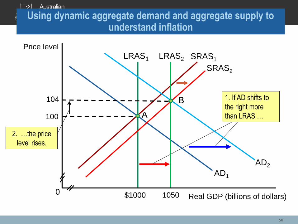
Using dynamic aggregate demand and aggregate supply to understand inflation

58

Analysing the dynamics• First figure: In the dynamic model, increases in the labour force

and capital stock as well as technological change cause long-run

aggregate supply to shift over the course of a year, from LRAS1 to

LRAS2. Typically these same factors cause short-run aggregate

supply to shift from SRAS1 to SRAS2. Aggregate demand will

shift from AD1 to AD2 if, as is usually the case, spending by

consumers, firms, and the government increases during the year.

• Second figure: The most common cause of inflation is total

spending increasing faster than total production. The economy

begins at point A, with real GDP of $1000 billion and a price level

of 100. An increase in potential GDP from $1000 billion to $1050

billion causes LRAS to shift from LRAS1 to LRAS2. Aggregate

demand shifts from AD1 to AD2. Because AD shifts to the right by

more than the LRAS curve, the price level in the new equilibrium

rises from 100 to 104. 59

“Keynesian” AD-AS• The AD-AS model we are studying has ‘Keynesian’ roots.

• We’ve already seen the relationship between AE and AD and the

fact that AD slopes downward because of macro effects on

C+I+G+NX through changes in the price level.

• In this synthesis model (AD-AS) there are actually some quite

complex monetary-real dynamics and interactions that are not fully

described analytically or explained, though we do put out some

plausible explanations for the effects. Particularly complicated is

the role of money – cash – in consumer behaviour. We have

spoken of wealth effects (which is sometimes called the Pigou

Effect after the neoclassical economist A.C. Pigou).

• But Keynes went further to say that as the price level falls, the real

value of money balances held increases, increasing real

purchasing power of consumers stimulating C. Money is a form of

wealth but much more tied to daily transactions.60

• Here is what Keynes himself said in the General Theory

about the relationship, in aggregate, between supply and

demand:

• “…the classical economists have taught that supply

creates its own demand; —meaning by this in some

significant, but not clearly defined, sense that the whole of

the costs of production must necessarily be spent in the

aggregate, directly or indirectly, on purchasing the

product.”

• Keynes then recasts this logic to say that “..supply creates

its own demand in the sense that the aggregate demand

price is equal to the aggregate supply price for all levels of

output and employment.”

61

Says Law• Classical economists, using a concept called Says Law

(named after Classical Economist Jean-Baptiste Say), held

that whatever was produced would be consumed, mainly

because of circular flow (i.e. factors are paid to produce

and they will spend what they earn to buy that total output).

• Keynes summarised this as “Supply creates its own

demand” (though Say himself did not use this phrase).

• But Keynes argued that supply is largely driven by the

expected extent of future demand, at least in many

circumstances and thus held that demand creates its own

supply. In other words if suppliers mis-estimate future

aggregate demand it is possible that some output might

remain unconsumed – a ‘general glut.’

62

• The AD-AS model is a synthesis of Keynes views and neoclassical models in several senses:

• (1) It is assumed the long-run equilibrium will always hold (neoclassical view) but that short-run deviations are possible and must be explained (inspired by Keynes).

• (2) Money is neutral in the long-run (neoclassical) but not in the short-run (inspired by Keynes but now accepted for different reasons by differing and even opposing schools –Keynesian, Neo-Keynesian, New Classical)

• (3) Both (aggregate) ‘supply’ (SRAS) and ‘demand’ (AD) determine output in the short-run (Keynesian) but only supply (LRAS) determines output in the long-run (neoclassical – Say’s Law holds).

• (4) Economic agent expectations (C and I) have short-run impact on output and prices (Keynesian) but not in the long run (neoclassical).

63

Poles of opinion• This sets us up for our potted history of macroeconomic

thought next week. Oversimplifying, current macro-economics

can be seen as split into two camps:

• (1) There are those who believe Says Law, neutrality of

money and equilibrium generally holds – in the long-run

always but sometimes even in the short-run.

• (2) Those who dispute this – sometimes even in the long-run.

• And there is whole range of attitudes in between.

• Post-GFC we seem to be operating in an overall Keynesian

intellectual framework with multiple strains of other models

thrown in. We will consider the evolution of this thought in

more detail next week.

64

macroeconomics 1 (econ1102)

Documents