Macroeconomic Theory Lecture 7

Antoine Godin Stephen Kinsella

October 23, 2014

Today: Real Business Cycle and New Keynesian Models.Key Reading: Romer, Chapter 5, Ball, Mankiw, Romer

I NK & RBC

I A ’flavour’ of DSGE.

Back to the 1970sI The Lucas critique: Macroeconomists should build structural

models, i.e. models where the agents behavior is invariantwith respect to policy/Microeconomic foundations/GeneralEquilibrium

I No distinction between micro and macro: Economic theory.I Explicitly dynamic models from the outset, implies a need for

Dynamic optimizationI Need for a theory of expectations formation. The Rational

Expectations Revolution of the 1970s is the logical outcome ofLucas research program

I The Methodological Proposal: New analytical andcomputational instruments (Lucas/Stokey and Prescott,Kydland and Prescott)

I A new equilibrium concept: recursive equilibrium and “from apoint to a path” type solutions.

I Importance of expectations in the design of policyexperiments. Nice because explicit welfare analysis. Astochastic description of the economic system.

Motivation

I Must allow for leisure/labour tradeoffs, motivating whyunemployment could exist within an equilibrium model.

I Fluctuations in factor productivity become the predominantcause of fluctuations in business activity.

I RBCs do well explaining co-movements in output,consumption, investment, employment. But three issues:

1. Labor supply elasticity.2. Productivity shocks and their frequency.3. Monetary policy shocks.

Basic Setup, 1/2.

I A Solow model in a dynamic optimisation framework

I Savings rate is no longer constant

I TFP shocks (i.e. the A matrix gets whacked)

I Policy uncertainty

Basic Setup, 2/2.

I A Central planning problem.

I As before, with set up problem, derive FOCs.

I Derivation and interpretation very standard.

I impose balanced growth conditions via log-linearisation

I return to FOCs

I Evidence on technological progress?

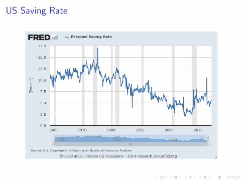
US Saving Rate

Variables

I t, time

I y output

I A technology level (exogenous)

I L, labour

I K , capital

I c consumption

I I investment

I w wage

I r interest rate

Baseline model

I See Romer pg 195-199.

I Production function is Cobb Douglas: Yt = Kαt (AtLt)

(1−α).

I Output divided into consumption C, government spending G,investment I. Depreciate at δ, soKt+1 = Kt + Yt − Ct − Gt − δKt .

I labour and capital get paid their marginal products,population grows exogenously. This is a market-clearing world.

I Household maximises U =∑∞

t=0 e−ρtu(ct , 1− lt)NtH

I Let c = C/N and l = L/N. Assume u() is log linear accordingto: ut = ln ct + b ln(1− lt)

I Technological disturbances are autoregressive:ln At = ρAt−1 + εA,t ..

I Shocks to government spending are also autoregressive:Gt = ρGGt−1 + εG ,t

Maximisation

I Form the Largrangian: L = ln c + b ln(1− lt) + λ(wl − c).

I FOCS: 1c − λ = 0 and −b

1−l + λw = 0

I A bit of algebra yields −b1−l + 1l = 0.

I How to read this? Note we’re actually solving a sequence ofstatic optimisation problems rather than a dynamic one.

Solution(s)

I Find the deterministic steady state (where ε = 0)

I Linearise all equations around the steady state

I Get the linearised solution of the form xt = Axt−1 + Bεt .,where x is the vector of all variables in the model. Thematrices A and B are the outcome of the model’s solution.

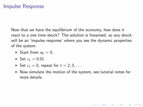
Impulse Response

Now that we have the equilibrium of the economy, how does itreact to a one time shock? The solution is linearised, so any shockwill be an ’impulse response’ where you see the dynamic propertiesof the system.

I Start from x0 = 0.

I Set ε1 = 0.01.

I Set εt = 0, repeat for t = 2, 3, . . ..

I Now simulate the motion of the system, see tutorial notes formore details.

Issues with RBCSI If all the important shocks are productivity shocks, then

worker hours and productivity should move together.I Thus productivity should be highly positively correlated with

output and hours. In the real world, the correlation is negative(if at all).

I Need for an highly elastic labour supply translates into seriouslabour market problems. The increase in productivitytranslates to an increase in hours worked and to an increase inreal wages. The effect on the real wage is relatively strongerthe lower is the elasticity of labor supply. In the extreme caseof a fixed labor supply all the increase in labor demand wouldtranslate into an increase in the real wage.

I There is no evidence of the large, economy-wide disturbancesthat drive these models.

I The models do not account for the periodicity of cycles. Theydo not match reality at all because they offer only weakexplanations for the propagation of the effects through time.

Now for a bit of context

Mkts clear? Mkts clear?

Yes. Classical No. KeynesianMarket Labour Friedman Sticky wage (eff. wage)Imperfection Product Lucasian islands Menu costs, other excuses.

Moving on. Models with Sticky Prices

I Contrary to the RBC type models which are dynamicequilbrium models with smoothly adjusting prices for capitaland labour, another school of economists has alwaysemphasized the ‘sticky’ nature of price movements.

I These guys came to prominence in the 1980s are are calledthe New Keynesians. Big paper: Clarida et al, 1993

I Keynesian arguments based upon rational expectations andmicroeconomic foundations. This deeply annoys anothersplinter group called ‘post-Keynesians’, but there are manyothers annoyed by these assumptions.

I These models usually take the form of

1. Contracting models2. Sticky price models based upon transactions cost or menu costs3. Efficiency wage models.

I They differ from RBC type modelers in their treatment ofmicro-policy and monetary policy.

Modeling issues

I An optimizing model of households and firms. Requires aproduction function, usually labour first.

I Differentiated goods and monopolistic competition. Allowssuppliers ability to set prices.

I Sticky price adjustment, obviously.

I Provide a mechanism for price level determination via interestrate rules of the type used by central banks. So a big focus onstuff like Taylor rules, etc.

I Model focuses on interest rate policy which is counter to thetraditional focus on changes in base money. Squares withactual practice.

I CB decision-makers mainly discuss changes in the nominal,overnight interbank interest rate target, leave manipulationsof base money to achieve those targets to trading specialists.

I Policy is rule-based.

Wicksellian solution

Knut Wicksell defined many of the major issues inmacroeconomics. He proposed setting nominal interest rates tostabilise the price level, so

it = i + θpt (1)

or

∆it = φπt (2)

Where pt is the log of the price level and πt = pt − pt−1..

Taylor

More modern interest rate rule relate the nominal interest ratetarget to the inflation rate rather than the price level, and alsooften add output stabilization as a goal.

it = i + πt + θπ(πt − π) + φy (yt − y) (3)

Here i is the target interest rate, π is the target inflation rate.yt − y is the output gap.(Another way to think about the rule is: Target Fed Funds =Inflation + Target Real Rate + param1*(Inflation Gap) +param2*(Output Gap).)The Taylor rule (and its many variants) do reasonably well atcharacterising movements in interest rate targets.

US Data on Taylor rulesSee: http://research.stlouisfed.org/publications/mt/page10.pdf

Data on Wage Stickiness: Wages *are* stickyLe Bihan, Montornes, and Heckel. 2012. “Sticky Wages: Evidence from QuarterlyMicroeconomic Data” American Economic Journal: Macroeconomics, 4(3): 1-32

Simple Model from Dixit and Stiglitz

I Only consumption goods here.

I Consumers maximize U(Yt) over a continuum of goods.

I So:

Yt = (

∫ 1

0Yt(i)

θθ−1 )

I they demand in the form

Yt(i) = Yt(Pt(i)

Pt)−θ

I Here P is a price index defined as

Pt = (

∫ 1

0Pt(i)1−θdi)

11−θ

Introducing price rigidity via Calvo

I Assume that at any moment some fraction 1− α of firms canchange their prices but everyone else has to keep theirs thesame–this is a menu cost assumption.

I Then otherwise firms are all the same.

I the price level then evolves according to

Pt = ((1− α)X 1−θt + αP1−θ

t−1 )1

1−θ

I Here X is the price set by those who can reset what theychoose.

I This then gets rewritten as

P1−θt = (1− α)X 1−θ

t + αP1−θt−1

Solving the NK Model

I Like RBC models it is done via log linearisation and then fairlystandard dynamic programming.

I The firms have to pick a set of prices relative to their costfunctions over time.

{pt} = βEtπt+1 +(1− α)(1− α ∗ β)

α(mct − pt)

Ye Wha?

I The New Keynesian Phillips curve relates price movements tomarginal cost (mc) and prices, which are themselves functionsof the output gap mct − pt = ρ(yt − y∗t )

I Here y∗t is the output the economy would produce if it had noinflation band all the factors of production were being usedoptimally.

DSGEs: Introduction

I Dynamic Stochastic General Equilibrium (DSGE) models arethe dominant modeling method in macro today. Regardless ofwhether you think these models are great or not, it isimportant you know what these are.

I A continuum of infinitely-lived agents (households and firms)solve intertemporal optimizing problems to choose how muchto consume, to work, to accumulate capital, to hire factors ofproduction and so on.

I Idea is to use the welfare of private agents (in fact, of therepresentative agent) as “a natural objective in terms of whichalternative policies should be evaluated”. (Woodford 2003,12).

Hubris?

“The state of macro is good”

(IMF Chief economist Olivier Blanchard, The state of macro,NBER WP14259, August 2008)

“Over the last three decades, macroeconomic theory andthe practice of macroeconomics by economists havechanged for the better. Macroeconomics is now firmlygrounded in the principles of economic theory”

(V. V. Chari and P. Kehoe (2006), Modern macroeconomics inpractice: how theory is shaping policy, Journal of EconomicPerspectives, Fall, pp. 328)

Using the Solow model to understand business cycles

I Basic Question: can the Neoclassical growth model be used tostudy business cycles, following Brock (1974)?

I Kydland and Prescott (1982): Yes, if you use stochastictechnology shocks with rational expectations.

I agent behaviour in the RBC model was governed by theoptimisation under uncertainty framework straight from themicro-economist’s toolbox.

I Problem: optimisation in the Neoclassical growth model yieldsnon-linear behaviour.

I Solution: linearise the model about the steady state of thesystem and consider an approximate solution viasimulation/calibration.

I More technically: a first-order approximation to theequilibrium conditions around the non-stochastic steady-stateto study the behaviour of endogenous variables in response tosmall stochastic perturbations to the exogenous process.

Next steps

I Calibration step. This involves choosing parameters on thebasis of long-run data properties and judgment (sometimesguided by microeconomic evidence).

I Judicious parameter selection is required.

I Cutting edge DSGEs use Bayesian methods (see Smets andWouters (2012, 2013).

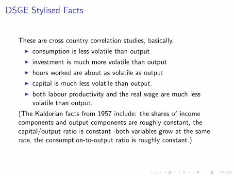
DSGE Stylised Facts

These are cross country correlation studies, basically.

I consumption is less volatile than output

I investment is much more volatile than output

I hours worked are about as volatile as output

I capital is much less volatile than output.

I both labour productivity and the real wage are much lessvolatile than output.

(The Kaldorian facts from 1957 include: the shares of incomecomponents and output components are roughly constant, thecapital/output ratio is constant -both variables grow at the samerate, the consumption-to-output ratio is roughly constant.)

A baseline DSGE

There is a perfectly competitive economy containing arepresentative household that maximizes utility given an initialstock of capital. The household simultaneously participates in thegoods, capital and labour markets. The economy also contains arepresentative firm, which sells output produced from capital,labour and technology according to

Yt = (AtNt)αK 1−α

t

Here Y is output, A is technology, N is the labour hours worked, Kis the capital stock, and 0 < α < 1.Capital accumulates according to

Kt+1 = (1− δ)Kt + Yt − Ct

Here δ represents depreciation while C is consumption.

Basic Setup

The household has log utility in consumption and power utility inleisure, so”

∞∑i=0

βi [log(Ct+i ) + θ(1− Nt+i )

1−γ

1− γ]

Here the elasticity of intertemporal substitution of leisure isσ = 1/γ and β is the discount rate.Firms invest according to the usual marginal assumptions. Thereturn on capital is

Rt+1 = (1− α)(At+1Nt+1

Kt+1)α + (1− δ)

First order conditions

1

Ct= βEt

Rt+1

Ct+1

and

θ(1− Nt)−γ =

Wt

Ct= α

AαtCt

(Kt

Nt)1−α

the marginal utility of leisure is set equal to the real wage Wttimes the marginal utility of consumption. Given a competitivelabour market, the real wage also equals the marginal product oflabour. This reflects the between-periods aspect of the problem, sothat labour supply is dictated by intertemporal substitution.

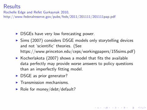
ResultsRochelle Edge and Refet Gurkaynak 2010,http://www.federalreserve.gov/pubs/feds/2011/201111/201111pap.pdf

I DSGEs have very low forecasting power.

I Sims (2007) considers DSGE models only storytelling devicesand not ‘scientific’ theories. (Seehttps://www.princeton.edu/ceps/workingpapers/155sims.pdf)

I Kocherlakota (2007) shows a model that fits the availabledata perfectly may provide worse answers to policy questionsthan an imperfectly fitting model.

I DSGE as prior generator?

I Transmission mechanisms.

I Role for money/debt/default?

Applications: Solving DSGE Models in practice andcomparing them to Agent-Based models.

1. Macroeconomic Policy in DSGE and Agent-Based Models

2. Real wages and monetary policy: A DSGE approach

3. RBCs and DSGEs: The Computational Approach to BusinessCycle Theory and Evidence

4. Ho’s lecture notes on DSGEs

5. Recent Developments in Macroeconomics: The DSGEApproach to Business Cycle in Perspective

Review of DSGE models

I Based on RBCs with real world data.

I Designed to provide welfare comparisons of varying importantpolicy parameters

I Explicitly equilibrium models, see previous lecture forcriticisms.

I Biggest criticism post-2008: the RBC/DSGE models areempirical failures, specifically with respect to the real effectsof monetary disturbances and financial frictions.

I much work has been done by the DSGE community post 2008to rectify these lacunae.

What is the point of all of this complexity?

I Latest and greatest models are very complicated, eg. Smetsand Wouters (2003, 2008), Christiano et al, 2005.

I Big plus is microeconomic foundations of these models. Butalso a big minus if you consider the series of problemsidentified with maximising behaviour over the last 30 years bybehavioural economists.

The ECB’s DSGE Model

I Based on Smets and Wouters (2007)

I A BVAR approach, See Christoffel et al. (2010)

...the new generation of DSGE models provides aframework that appears particularly suited forevaluating the consequences of alternativemacroeconomic policies. (Christoffel et al., 2010:3)

I Really?