1

Macroeconomic Policies and Housing Market in Taiwan

Shiou-Yen Chu

Department of Economics,

National Chung Cheng University

Email: ecdsyc@ccu.edu.tw

October 2016

Abstract

This paper develops a dynamic stochastic general equilibrium (DSGE) model that analyzes the transmission

mechanisms of a real estate transfer tax and other macroeconomic policies on Taiwan’s housing market. Our

model matches the volatility of Taiwan’s housing prices and housing transactions during 2011-2015, when the

loan-to-value ratio was reduced and a transfer tax on real estate was collected. The calibration results indicate that

imposing a residential property tax or raising interest rates effectively curbs speculative housing transactions and

has prolonged effects on taming housing prices over time. Transfer tax imposition or a decrease in the

loan-to-value ratio has short-lived effects on moderating housing markets.

JEL classification: E52, F41, R21

Keywords: Collateral constraint, property tax, transfer tax, speculation

2

1 Introduction

The global financial crisis that began in 2008 increased policymakers’ attention on the

housing market. Several countries have adopted macroprudential polices to ensure the

sustainability and resilience of their housing markets. Behind these policies lies the theory that

housing prices are more sensitive to monetary policy shocks than consumer prices (Iacoviello

2010; Iacoviello and Neri 2010). Hence, the monetary authority (alone or with fiscal authority)

can use policy instruments to stabilize housing prices and economic activities.

The Central Bank of the Republic of China (Taiwan) and the Ministry of Finance have

collaborated on mitigating the rise in housing prices since 2010. Their policies include

reducing limits on maximum loan-to-value (LTV) ratios from 60% to 50% for luxury

properties, the third individually owned property, and corporate real estate. Also, “luxury

properties” were reclassified with lower threshold values1, and an excise tax was levied on

non-owner-occupied residential properties bought and sold within two years. The latter was

legislated in the Specifically Selected Goods and Services Tax Act and went into effect on

June 1st, 2011. Under this tax policy, the property sellers are obligated to pay 15% and 10% of

the full selling prices of houses sold within a year and two years of purchase, respectively.

Hereafter, we will refer to this excise tax as a real estate transfer tax in the context2.

1 The threshold values for luxury properties were lowered from NT$80 million to NT$70 million in Taipei City,

from NT$80 million to NT$60 million in New Taipei City, and from NT$50 million to NT$40 million in other

districts. 2 This real estate transfer tax policy ended on December 31

st, 2015. Beginning on January 1

st, 2016, the capital

gains from transferring housing and land are consolidated as taxable income and calculated on the basis of market

values. In the old tax scheme, they were taxed separately and at assessed values which are usually below their

market prices. Furthermore, non-Taiwanese residents are obligated to pay a flat 35% tax rate for selling property

3

Taiwan’s real estate transfer tax is distinctive for two reasons. First, different from a

capital gains tax, it considers the full value of the transaction as the tax base. Second, unlike

the stamp duties conducted in Hong Kong and Singapore that also aim to curb booming

housing markets, sellers instead of buyers are designated as taxpayers. The two tax brackets

are cut off by the holding period of the property but not by the transaction value of the

property.

Figure 1 presents the number of home ownership transfers during 2005Q1-2016Q23 in

Taiwan. The number of ownership transfers through transactions experienced two sustained

declines during 2008Q2-2009Q1 and 2010Q4-2012Q1. The first drop was the consequence of

the U.S. subprime mortgage crisis and the second drop might have been an effect of the

announced changes in the real estate transfer tax policy. Meanwhile, transactions involving

first registration of building ownership fell below 40,000 in 2008Q2 and have fluctuated

within the range of 20,000 to 40,000 since then. Figure 2 plots the housing price indexes for

Taipei City, New Taipei City, and Taiwan from 2005Q1 to 2016Q24. Taipei city is Taiwan’s

capital city and has a large number of luxury properties, while New Taipei city is the most

densely populated city in Taiwan. The housing prices in Taipei slightly dropped since the Real

Estate Transfer Tax Act went into effect in June 2011. Nevertheless, sustained decreases in

owned for more than one year. For Taiwanese residents, the tax rates for transferring real estate decrease from 35%

to 15% as the holding period lengthens from one year to over ten years. 3 The data were obtained from the Monthly Bulletin of Interior Statistics, August 2016, Ministry of the Interior.

(http://sowf.moi.gov.tw/stat/month/list.htm) 4 The data were obtained from the website of Sinyi Realty Inc. (http://www.sinyi.com.tw). The first quarter in 2001

was chosen as the base year.

4

housing prices did not appear until 2014Q2. The housing prices for Taipei City, New Taipei

City, and Taiwan during 2011Q2 and 2014Q2 generally showed positive trends.

Taiwan’s transfer tax imposition gives a natural experiment for observing the effect of a

one-time tax policy on housing markets. The insufficient empirical data (only 19 quarters)

limits the methodology that can be conducted to evaluate the policy effects. The purpose of

this paper is to provide a theoretical framework that analyzes the transmission mechanism of a

real estate transfer tax along with other macroeconomic policies for Taiwan’s housing market.

Our model intends to capture the fact that owning real estate in Taiwan is considered as a

token of wealth accumulation. The Taiwanese government aims to increase homeownership by

providing regular households fairly and reasonably priced properties. Nevertheless,

speculators purchase additional housing not as a principal place of residence but as an

investment target for generating income. Excess demand fuels property price escalation and

makes housing unaffordable to regular households. Macroeconomic policies are implemented

to mitigate speculative activities in the housing market.

We develop an open-economy dynamic stochastic general equilibrium (DSGE)

framework. Our model distinguishes two types of agents: borrowers and savers. They are both

homeowners. Borrowers (speculators) are less patient and collateral-constrained when they

would like to purchase additional housing for investment purposes. The reason for introducing

two kinds of households is stated in Iacoviello’s (2005) and Iacoviello and Neri’s (2010)

5

studies. Higher asset prices resulting from demand shocks expand debtors’ borrowing capacity

against collateralized asset. Higher consumer prices reduce the real value of debtors’

obligations and promote their net worth. Both effects strengthen collateral-constrained

households’ spending capacity. Hence, the presence of collateral-constrained agents magnifies

the impact of housing prices on overall consumption.

Moreover, our model classifies two kinds of housing: residential housing and investment

housing. The former consists of owner-occupied properties that provide services for borrowers

and savers. The latter is characterized as speculative housing in three aspects. First, it does not

directly provide utility of housing services since speculators do not live in it. Investment

housing is not a speculator’s primary residence. Second, investment housing is an input in the

production of residential housing. Speculators purchase investment housing, namely

unfinished housing units, and make renovations. Investment housing is converted into

habitable units through production technology and then put on the market for sale. Third, the

expected prices of investment housing affect a speculator’s borrowing availability. Only

borrowers can purchase investment housing and pledge it as collateral for loans. Two kinds of

taxes are imposed on the home properties. Both agents pay property taxes for their primary

dwellings. Borrowers pay a transfer tax as a percentage of the transaction price when selling

investment housing to the producers of residential housing.

The model is evaluated by property tax shocks, transfer tax shocks, interest rate shocks

6

and loan-to-value shocks. Our results indicate that our model in response to transfer tax shocks

and loan-to-value shocks matches the volatility of Taiwan’s housing prices and housing

transactions during 2011Q2-2015Q4, when the loan-to-value ratio was reduced and a transfer

tax was collected. Property tax imposition or an interest rate hike curbs speculative housing

transactions and has prolonged effects on taming housing prices. Relatively, transfer tax

imposition or loan-to-value reduction instantly depresses investment housing prices, but not

investment housing transactions.

Both property tax shocks and interest rate shocks alter the relative prices of current

tradable consumption, future tradable consumption, and residential housing. A property tax

raises the holding cost for residential housing and decreases speculator’s purchase intent for

investment housing. With regard to interest rate shocks, the dominating substitution effect

resulting from an interest rate hike shifts borrowers’ and savers’ resources from current

tradable consumption to current residential housing and to future tradable consumption.

Strengthened current demand for residential housing initially upholds investment housing

prices, while increasing borrowing costs and the associated limited funding liquidity

discourage borrowers from purchasing investment housing. One caveat of influencing housing

markets with monetary policies is that changing interest rates adds variability in households’

consumption.

Different from property tax shocks and interest rate shocks, transfer tax imposition and

7

loan-to-value ratio restrictions primarily affect borrowers’ intertemporal allocation of tradable

consumption and intra-temporal allocation between tradable consumption and investment

housing. Both shocks weaken borrowers’ demand for residential housing, leading to declines

in residential housing prices and investment housing prices. Loan-to-value shocks produce

similar but less substantial responses in consumption, housing prices, housing transactions and

output than transfer tax shocks.

Investment housing plays an important role in the transmission mechanism of exogenous

shocks in our model. Although all the shocks dampen residential housing prices, they generate

different responses in investment housing prices and transactions. The responses of investment

housing stock are closely related to the expected demand of residential housing consumption.

Transfer tax and loan-to-value shocks do not immediately depress investment housing stock.

This is because a transfer tax is imposed on the sale of previous-period investment housing

stock, while loan-to-value shocks impact speculators’ borrowing availability that is associated

with the future price of investment housing. As long as speculators perceive that a transfer tax

and a lower loan-to-value ratio are short-term policies and foresee climbing housing prices,

they still purchase investment housing and hold down for future residential housing

production.

Our study bridges two strands of research. One strand of research5 empirically documents

5 Benjamin et al. (1993), Dachis et al. (2012), Best and Kleven (2013), Besley et al. (2014), as well as Kopczuk and

Munroe (2015).

8

the microeconomic effects of a real estate transfer tax on the housing market under the

assumption that the government imposes a real estate transfer tax for revenue-generating

purposes. The other strand of research6 incorporates a housing sector in a DSGE model

irrespective of fiscal policy shocks in order to discuss macroeconomic phenomena. More

recently, the effects of fiscal policy on the housing market have gained more attention.

Alpanda and Zubairy (2016) examine the effects of several housing-related tax policies

excluding transfer tax policy on macroeconomic variables. Funke and Paetz (2016) analyze

the effects of nonlinear loan-to-value ratios and nonlinear property transfer taxes (stamp duties)

on Hong Kong’s housing prices in a DSGE framework. In line with the abovementioned

studies, our theoretical framework suggests that tax policies or monetary policies moderate

housing prices but generate different policy effects in terms of duration and magnitude.

However, different from Funke and Paetz (2016), our paper is motivated by Taiwan’s peculiar

experience of real estate tax imposition and emphasizes the role of speculative housing. In

addition to being characterized by the level of impatience and the presence or absence of

collateral constraint, savers and borrowers in our model face different real estate transfer tax

rates. Our model also considers a rich set of macroeconomic policy shocks on dampening

housing prices and housing transactions.

The remainder of this paper is organized as follows. Section 2 provides a brief review of

6 Aoki et al. (2004), Iacoviello (2010), Iacoviello and Neri (2010), Funke and Paetz (2013), Stark (2015), and

Piazzesi and Schneider (2016).

9

related literature. Section 3 describes our model. Section 4 presents calibration results, and

section 5 concludes.

2 A Brief Review of Related Literature

2.1 Real Estate Transfer Tax

Benjamin et. al (1993) utilize real estate data consisting of 352 single-family home sales

from February 1987 through June 1989 in Philadelphia to discuss the valuation effects of a

transfer tax. Nominally the tax payment is distributed between sellers and buyers. Due to a

short-time period dataset and the evidence that used home transactions are relatively larger

than new home transactions, they assume that the supply of housing is inelastic. This creates a

strict hypothesis that the seller will completely absorb the tax burden along with a decline in

the home prices by the full amount of the tax. A rejection of the hypothesis leads to two

implications. First, the housing supply is not perfectly inelastic. Second, mortgage markets are

not perfect. Households become more down-payment constrained in response to additional

taxes, accordingly reducing housing demand and prices. Their second hypothesis lies on the

information issue that home prices should decrease on the date of bill passage in order to avoid

the tax liability. Their results indicate that home prices fall as expected, but not statistically

significantly.

Dachis et. al (2012) employ a data set of 139,266 single-family houses in the greater

10

Toronto area between January 2006 and August 2008 to estimate the impact of a land transfer

tax on the housing market. Their methodology is a hybrid of a regression discontinuity model

and differences-in-differences estimation. Their findings show that the new tax policy results

in reduced transaction volume and lower home prices. Most importantly, it causes a substantial

welfare loss. The authors suggest that the government should consider revenue-equivalent

alternatives to the land transfer tax.

Best and Kleven (2013) examine the impact of UK property transaction taxes (also

known as the Stamp Duty Land Tax, SDLT) on the housing market from 2004-2012. The

statutory taxpayer of the SDLT is the buyer, whose tax liability is calculated as a proportional

tax rate times the entire transaction price. The tax rate is constant within each bracket. The

presence of the SDLT alters the cost of homeownership. Since it cannot be paid with mortgage

loans, it creates excess pressure for liquidity constrained buyers. The authors estimate the

elasticity of housing prices with respect to the marginal tax rate by using the notches at the

cutoff prices that are discontinuities in the overall tax liability. Their results indicate that

housing prices and transaction activities are sharply responsive to tax changes, supporting the

implementation of fiscal stimulus on economic recovery from recessions.

Similarly, Besley et. al (2014) estimate the effect of a UK stamp duty holiday on housing

prices and transactions during 2008-2009. Their findings show that a stamp duty holiday

generates lower property prices and a significant but short-lived increase in transaction

11

volumes. They also calibrate a simple bargaining model and conclude that buyers’ tax liability

was reduced by 60% during the holiday window.

Kopczuk and Munroe (2015) examine the consequences of a transfer tax levied on the

sales of houses and apartments in New York and New Jersey exceeding $1 million. By law the

buyers are responsible for paying the so-called “mansion tax” in New York state and New

Jersey. Their paper focuses on the tax incidence, price distortion between asking price and sale

price, as well as search frictions in response to policy changes. They conclude that a transfer

tax increases inefficiency in the house search process.

2.2 DSGE models with a Housing Sector

Aoki et al. (2004) examine the financial accelerator effect of homeowners’ borrowing

funds from financial intermediaries to purchase houses. Homeowners rent housing services to

tenants and also provide tenants “transfers” for consumption. A composite of homeowners and

tenants in the model captures the fact that home equity can be used to finance both

consumption and housing investment. As home prices go up and the transfer payments stay the

same, homeowner’s net worth will increase, leading to lower future borrowing costs. Their

results show that monetary policy shocks have substantial impacts on housing investment,

housing prices and consumption.

Iacoviello (2010) summarizes several facts about housing markets and the macroeconomy.

First, consumption expenditure and housing investment move procyclically with housing

12

wealth. Second, housing wealth accounts for a larger share of national wealth than GDP. Third,

variables in the housing market, such as residential investment and housing price inflation, are

more volatile and proceed in advance compared to variables in other markets.

Iacoviello and Neri (2010) propose that nominal rigidity either in prices or wages

propagates the transmission of monetary shocks to housing consumption. The presence of

collateral-constrained borrowers amplifies the effect of housing prices on aggregate

consumption since impatient agents have a greater propensity to consume at the margin than

patient agents. Hence, to quantify the housing demand shocks and monetary policy shocks on

the economy, nominal rigidity and collateral-constrained households are two essential

elements in a DSGE model. In their paper, housing preference shocks, monetary shocks, and

technology shocks are analyzed to capture some of the business cycle facts. Three findings are

summarized here. First, increasing housing demand, denoted as a shift towards housing

preference, will boost housing prices and collateral-constrained households’ borrowing

capacity. Tightening money supply, denoted as an increase in nominal interest rates, depresses

aggregate demand and housing prices. Last, an improved productivity in the goods sector

increases housing prices while a positive technology shock in the housing sector decreases

housing prices.

Funke and Paetz (2013) construct a two-agent, two-sector, open-economy DSGE model

to examine the impact of housing price cycles on Hong Kong’s economy. In their model, the

13

domestic country interacts with the foreign country through two channels. First, residential

and non-residential consumption goods are both tradable. Second, domestic savers can trade

bonds with foreign households to completely share the country-specific risks. The model is

calibrated with households’ preference shocks, loan-to-value shocks, sector-specific cost-push

shocks, and sector-specific technology shocks. Their findings indicate that Hong Kong’s

property prices are mainly driven by the intra-temporal marginal rate of substitution between

residential and non-residential goods. Shocks on the loan-to-value ratios do not significantly

affect housing prices.

Stark (2015) constructs a two-agent, two-sector, and closed-economy DSGE model to

study the relationship between home prices and unemployment during the U.S. great recession.

He finds that declining housing prices associated with lower home equity creates

unemployment, particularly for the collateral-constrained households. A decrease in home

prices restricts the impatient households’ borrowing availability along with their geographical

mobility.

Alpanda and Zubairy (2016) develop a model consisting of two sectors (housing and

non-housing goods) and three types of households (patient, impatient, and renter households)

to assess the welfare consequences of several housing-related tax policies, such as an increase

in the property tax rate, elimination of the mortgage interest deduction, elimination of

depreciation allowance for rental income, elimination of the property tax deduction, and

14

taxation of imputed rental income on macroeconomic variables. Welfare consequences are

measured by the output loss, lifetime consumption-equivalent loss, and generated tax revenue.

They find that taxation of imputed rental income from owner-occupied households and the

elimination of the property tax deduction cause the greatest output losses. The elimination of

the mortgage interest deduction can effectively raise the most tax revenue per unit of output

loss.

Funke and Paetz (2016) analyze the effects of nonlinear LTV ratios and nonlinear property

transfer taxes on Hong Kong’s housing prices in a DSGE framework. The central bank is

assumed to adjust LTV ratios and tax rates responding to property price inflation over a

threshold value. Comparing the nonlinear policies with a linear Taylor-type LTV policy, their

results suggest that nonlinear property transfer taxes are more effective than nonlinear or linear

LTV policies in taming home prices. The dampening effect of nonlinear LTV policies becomes

intensified while that of nonlinear property transfer taxation becomes weakened as the number

of time periods for which the policy takes effect increases.

3 Our Model

Our model is a modified version of Iacoviello and Neri’s (2010) model. The economy is

assumed to consist of borrowers (speculators) and savers (patient households). There is an

equal number of borrowers and savers. Both borrowers and savers are homeowners.

Borrowers are less patient and collateral-constrained when purchasing additional properties for

15

investment purposes. Their borrowing capacity is tied to the expected future value of the

investment housing. Savers have accumulated sufficient wealth and are not credit-constrained.

Households share the same preferences, consuming a CES composite of domestic tradable

goods, foreign tradable goods, and non-traded goods (residential housing). Domestic firms in

the tradable goods sector produce intermediate goods with labor in a monopolistically

competitive market. Domestic firms in the housing sector produce intermediate goods with

labor and investment housing in a monopolistically competitive market. The final goods

markets in both sectors are assumed to be perfectly competitive. The presence of imperfect

competition creates market distortions and provides a rationale for the central bank to

implement monetary policy rules.

3.1 Borrowers

The preference of the representative borrower is defined over a composite consumption

of tradable goods

B

tC , non-traded goods B

tD and disutility of employment in two sectors

,

B

C tN and ,

B

D tN . The objective of the representative borrower is to maximize the expected

present discounted utility (1) subject to the budget constraint (3) and the collateral constraint

(4) in real terms.

Max

1 1

, ,

0 0ln ln

1 1

B BC t D tt B B

t t tt

N NE C D

(1)

16

11

,

11

,

1

1

B

tFC

B

tHC

B

t CCC (2)

2

1

1 1 2 1

1

1 1 1 (1 )2

t tB B B

t t t t t t t t t

t

K KC Q D D H K K

K

* * *11 1 1 , , , ,

, ,

1 1B

B B B Bt t tt t t t t t C t C t D t D t C

C t C t t

b S Tb r S b r b w N w N

P

(3)

* *

1 , 11 1 1B B

t t t t t t t t t C tr b r S b E K H , (4)

where is the borrowers’ discount factor, t is a housing preference shock and is the

elasticity of marginal disutility with respect to labor supply. is the elasticity of substitution

between domestic goods B

tHC , and foreign goods B

tFC , . is the steady-state share of

foreign goods in tradable goods consumption.

Non-traded goods, tD , include housing units as principle residences and their incurred

housing-related services. Borrowers also purchase housing units, tK , for investment purposes

and use them as collateral for loans. tK can be interpreted as the unfinished housing units and

considered as an input in the production function of residential housing. Hereafter, we will

name tD as residential housing and tK as investment housing. An increase in tK increases

the supply of residential housing and brings a positive wealth effect to speculators. tQ is the

relative price of residential housing or imputed rent, defined as , ,D t C tP P . tH is the relative

price of investment housing, defined as , ,K t C tP P . We assume that each unit of investment

housing incurs an additional resource cost. measures the magnitude of adjustment costs for

.st

C

17

tK . A greater hinders the accumulation of the stock of investment housing. The

government intends to impose two kinds of taxes on properties. 1t is the property tax rate

shock, and 2t is the transfer tax rate shock on the sales of investment housing

7.

Households hold domestic borrowing tCtt PBb , and foreign borrowing tCtt PBb ,

** .

An asterisk represents the foreign country. B

tr represents the domestic loan rate.

, , ,C t C t C tw W P and , , ,D t D t C tw W P represent the real wages in two sectors. tS represents

the price of the foreign currency in units of domestic currency. An increase in tS represents

the depreciation of domestic currency. 1,,, tCtCtC PP is the domestic inflation rate of

tradable goods. B

tT is the lump-sum transfer from the government to borrowers. t

represents the fraction of housing value that can be used as collateral. Monacelli (2009) and

Calza et al. (2013) refer to t1 as the down-payment rate. We follow Funke and Paetz

(2013) in using t as a proxy for the loan-to-value ratio shocks.

Let t and t t be multipliers for the budget constraint and collateral constraint,

respectively. The first order conditions are defined in equations (5)-(11).

t

tB

tC

, (5)

C, C,

1B

t tB

t

N wC

, (6)

D, D,

1B

t tB

t

N wC

, (7)

7 We assume that borrowers only hold investment housing for one period and must sell it in the next period. The

uncertainty arises in that agents do not know in which particular period policy shocks will occur.

18

1 , 1

11 1

BBtB t

t t t B

t C t

rCr E

C

, (8)

*

* 1

1 , 1

11 1

BBtB t t

t t t B

t C t t

rC Sr E

C S

, (9)

11 1

1

1 1 1t t tt t tB B B

t t t

Q QE

D C C

, (10)

1

1

t t

t t

t

K KH

K

1 1

1 2 1 1 1 , 121 1 1

t t t t

t t t t t t t t C t

t

K K K KH E H

K

. (11)

Equations (6) and (7) show the trade-offs between consumption and labor choice in

sectors tC and tD , respectively. Equation (8) is an intertemporal Euler equation. Equation (9)

derives the uncovered interest parity. Equation (10) states that the marginal benefit of

increasing an additional unit of residential housing at time t must equal the marginal utility

of tradable goods consumption at time t . The former consists of the marginal utility from

housing services and the marginal utility of tradable goods consumption from selling the house

at time period . Equation (11) states that the marginal cost and the marginal benefit of

increasing an additional unit of investment housing must be equalized. The latter includes the

increases in utility of more wealth associated with higher future housing prices and in utility

associated with greater borrowing capacity against home equity.

3.2 Savers

1t

19

Savers are assumed to be more patient than borrowers and are not collateral-constrained.

Their optimization problem is defined as follows.

Max

1 1

, ,

0 0ln ln

1 1

S SC t D tt S S

t t tt

N NE C D

(12)

1 11 1 1

, ,1S S S

t C H t C F tC C C

*

1 11 1S S S

t t t t t t t tC Q D D b S b

* *11 1 1 , , , ,

, ,

1 1S

S S S St t tt t t C t C t D t D t C

C t C t t

b S Tr r b w N w N

P

, (13)

where C

t t tb B P and * * C

t t tb B P are loans provided by domestic households and foreign

households with rates of return S

tr and *S

tr , respectively. S

tT is the lump-sum transfer from

the government to savers. Equation (13) represents savers’ budget constraint. The main

difference between (13) and (3) is that savers purchase housing mainly as principle residences,

not for investment purposes. tK is hence omitted here. The first order conditions for savers

are defined in equations (14)-(18). ~

is the savers’ discount factor. S

tr defines the rate of

return for deposits.

, C,

1S

C t tS

t

N wC

(14)

D, ,

1S

t D tS

t

N wC

(15)

1

, 1

11

SS t

t t S

C t t

Cr E

C

(16)

.st

20

1

*

1

1

S

t ttS

t t

r SE

r S

(17)

11 1

1

1 1 1t t tt t tS S S

t t t

Q QE

D C C

(18)

3.3 Retailers and Intermediate Goods Producers

Retailers combine intermediate goods with no additional inputs and sell final goods to

consumers in a perfectly competitive market. Retailer production is a

constant-elasticity-of-substitution aggregate of a continuum of intermediate producers. The

production functions for domestic retailers in the tradable goods sector and housing sector are

defined as

1

1 1 1

, ,0

( )l t l tY Y j

, ,l C D (19)

where refers to the elasticity of substitution between any two differentiated goods and is

assumed to be the same in both sectors.

Intermediate goods firms use different kinds of technology while producing tradable

goods and residential housing in monopolistically competitive markets. The production

functions for individual firms in sectors C and D are defined by equations (20)-(21). ,C tZ

and ,D tZ are the productivity shocks and are assumed to be identical for each firm. H is

the steady-state share of investment housing used in residential housing production.

, , ,( ) ( )C t C t C tY j Z N j

(20)

21

1

, , , 1( ) ( ) ( )H H

D t D t D t tY j Z N j K j

(21)

Each firm charges a price mark-up over its nominal marginal cost. Each period only a

fraction 1 − ϖ of all firms can adjust their prices. ϖ is a measure of the degree of nominal

rigidity. Each firm faces a constant elasticity demand curve given by equation (22). Equations

(23)-(24) represent the real marginal costs in two sectors. We assume that the nominal wages

in the two sectors are deflated by the aggregate consumer price index. This setting implies that

exchange rate changes will affect the real marginal costs in two sectors, since the aggregate

consumer price is composed of the prices of domestic tradable goods and foreign tradable

goods.

,

, ,

,

( )( ) l t

l t l t

l t

P jY j Y

P

, ,l C D (22)

, ,

,

,

C t C t

C t

C t

W PMC

Z (23)

, ,

,

,

11

D t D t

D t H H t

D t t

W PMC H

Z Q

(24)

3.4 The Banking Sector

The banking sector operates in a standard Dixit-Stiglitz monopolistically competitive

market. We assume that banks can transform the mortgage loans into securities with a

constant-return technology. These mortgage-based securities will be sold to domestic savers

and foreign savers for banks’ additional funding sources. Individual banks face a deposit

22

demand function (25) and a loan demand function (26).

,* *

, ,

S

j t

j t t j t t t tS

t

rb S b b S b

r

. (25)

,* *

, ,

B

j t

j t t j t t t tB

t

rb S b b S b

r

, (26)

where S

tjr , and B

tjr , are the interest rates offered by bank j to saving and borrowing,

respectively. *

,,

~~tjttj bSb is the total deposit (domestic and foreign) collected by each bank

j ; while *

,, tjttj bSb is the total borrowing (domestic and foreign) issued by each bank j .

represents the interest rate elasticity of demand for deposits and loans.

Each bank is assumed to maximize its expected present value of profit flows (27) subject

to deposit and loan demand functions. The last term in (27) represents the adjustment cost

incurred when the loan rate at 1t differs from that at t . The parameter Bk measures the

degree of interest rate adjustment cost. The banking sector has the same discount factor as

savers since we assume savers own banks. Equation (28) represents the banks’ balance sheet

constraint, indicating that loans issued to borrowers equal the level of savers’ deposits.

2

,* * *

0 , , , , , ,01

( ) 1 .2

BSj t iB S Bt B

j t i j t i t j t i j t i j t i t i j t i t i t i t i t iS Bit i t i

rC kE r b S b r b S b r b S b

C r

(27)

* *

, , , ,j t t j t j t t j tb S b b S b . (28)

We assume all banks make the same decisions. After substituting the bank’s balance sheet

into the profit function and imposing the symmetric conditions, we obtain

23

11 B B S

B t B t- tk r k r r (29)

3.5 Fiscal and Monetary Authorities

The real government budget constraint is defined as equation (30). The fiscal authority

owns the initial stock of investment housing, financing government purchases and transfer

payments with tax revenue from residential properties and proceeds from the sales of

investment housing8. The sales conducted by the government are assumed to be exempted

from the transfer taxes. The monetary authority operates the interest rate by responding to a

lagged policy rate, output gap and aggregate inflation. Let a lower case variable with a hat

denote the percentage deviation of a variable around its steady state. In terms of the deviation

from zero inflation, the interest rate rule can be expressed as equation (31). R is the weight

imposed on lagged policy rates. Y is the weight imposed on the inflation rate and output

gap. and Y are the coefficients of inflation and output gap, respectively, in the Taylor rule.

Equations (32) and (33) are the inflation adjustment equations for sectors C and D .

1 1 1 2 1 11 1 1 1B S

B B S S t tt t t t t t t t t t t t tC C

t t

T TQ D D D D H K H K K G

P P

(30)

1 , ,ˆ ˆ ˆ ˆ ˆ(1 ) 1S S

t R t R C t D t Y t tr r y u

. (31)

8 The fiscal authority has incentives to sell unfinished houses (investment housing) since residential property taxes

and transfer taxes are the only sources for generating government revenue.

24

, , 1 ,ˆ ˆ ˆ ˆ1 1C t t C t t C tE w z . (32)

, , 1 ,ˆˆ ˆ ˆ ˆ ˆ1 1 1D t t D t H t t H t D tE w q h z

. (33)

3.6 Equilibrium

Equations (34)-(38) represent the equilibrium equations in the model. In equation (34),

domestic production tY equals the sum of the following: domestic consumption of tradable

goods and residential housing services, resource costs of investment housing, government

purchases and exports of domestically produced goods. The foreign demand for domestically

produced goods is proportional to the foreign country’s aggregate income *

tY . Equation (35)

defines the terms of trade condition. With complete exchange rate pass–through, the imported

price of foreign goods equals the foreign currency price denominated in the domestic currency,

that is, *

,, tHttF PSP . We assume the foreign country is relatively larger than the home country,

so its consumer price inflation and producer price inflation are the same. Hence, *

, ,F t t C tP S P .

Equations (36)-(38) imply that the labor market and bond market are in equilibrium. Finally,

foreign households are assumed to have the same preferences as domestic households. The

individual intermediate goods producer’s production function in the foreign country takes the

same form as that in the domestic country.

1 11 1 1B S B B S S

t C t t t t t tY C C D D D D

2

1 *

12

t t

t C t t

t

K KG Y

K

(34)

25

tH

tCt

tH

tHt

tH

tF

tP

PS

P

PS

P

P

,

*

,

,

*

,

,

, (35)

, , ,

B S

C t C t C tN N N , (36)

, , ,

B S

D t D t D tN N N , (37)

* * 0t t t t t tb S b b S b . (38)

3.7 Exogenous Shocks

Productivity shocks in two sectors, housing preference shocks, tax rate shocks, monetary

policy shocks, loan-to-value shocks, foreign productivity shocks and exchange rate shocks are

assumed to be exogenous and follow an exogenous )1(AR process in equations (39)-(47). tm1 ,

tm2 , tm3 , 4tm , 5tm , 6tm , 7tm , 8tm and 9tm are assumed to be a serially uncorrelated

process with mean zero. is assumed to be less than 1.

, , 1 1ln lnC t C t tZ Z m (39)

, , 1 2ln lnD t D t tZ Z m (40)

1 3ln lnt t tm (41)

1 1 1 4ln lnt t tm (42)

2 2 1 5ln lnt t tm (43)

1 6ln lnt t tu u m

(44)

1 7ln lnt t tm

(45)

* *

1 8ln lnt t tZ Z m (46)

26

1 9ln lnt t tS S m (47)

4 Calibration Results

4.1 Parameters and steady-state values

Following previous literatures (Teo 2009; Huang and Ho 2012) that apply a DSGE

framework to Taiwan’s economy, the depreciation rate of housing is set to be 0.025. The

elasticity of substitution between any two differentiated goods is set to be 6, implying that

a price markup over marginal cost is 20%. The degree of nominal rigidity is set equal to

0.75, implying that the expected time between price adjustments is one year.

Based on Taiwan’s real data during 2000-2013, the discount factor ~

for savers is

pinned down to 0.9945, which implies an annualized deposit rate of 2.23%. The discount

factor for borrowers is 0.9467, which implies an annualized lending rate of 4.27%9. The

steady-state share of housing-related expenditure in total consumption is 0.23, and the

steady-state share of foreign goods in tradable goods consumption C is 0.5610

. The

non-labor share of housing production H is set to be 0.3011

. 𝐾 �̅�⁄ is set to be 0.02 based

on the average ratio of real residential investment to Taiwan’s real GDP during 2000-2013.

�̅� �̅�⁄ is set to be 0.17 based on the average ratio of real housing-related consumption plus the

9 In the steady state, β + �̅� = 1 (1 + �̅�𝐵)⁄ , β̃ = 1 (1 + �̅�𝑆)⁄ . 10 Housing-related expenditure includes the spending on residential services, water, electricity, gas, and other fuels, as well as furnishings, household equipment, and routine household maintenance. The average share of housing-related consumption over total household consumption during 2000-2013 in Taiwan was about 0.23. Due to data availability, we use the import-to-GDP ratio as a proxy for the share of foreign goods consumption in tradable goods consumption. The average ratio of imports of goods and services over GDP during 2000-2013 in Taiwan was about 0.56. 11 The average ratio of employees’ compensation in the sectors of furniture, manufacturing, real estate and ownership of dwellings during 2000-2013 was about 0.7.

27

gross capital formation for construction as well as real estate and ownership of dwellings to

Taiwan’s real GDP during 2000-2013. �̅�𝐷 �̅�⁄ is set to be 0.12 based on the average share of

Taiwan’s real GDP in the sectors of furniture, manufacturing, real estate and ownership of

dwellings during 2000-2013. 𝐶̅ �̅�⁄ is set to be 0.61 based on the average ratio of Taiwan’s

private consumption over its real GDP during 2000-2013. �̅� �̅�⁄ is set to be 0.0005 in order to

satisfy the steady-state real government budget constraint.

The central bank in Taiwan uses the discount rate as a monetary policy target. Hence, we

apply an ordinary least squares method on equation (31) with Taiwan’s discount rate, changes

of consumer price index, and output gap from 2000Q1 to 2013Q4 to determine the coefficients

in the Taylor rule. The output gap is defined as the deviation of seasonally adjusted real GDP

from its HP-filtered trend. The results show that all the coefficients 0.95R , 0.77 ,

and 1.13Y are statistically significant.

The elasticity of substitution between domestic goods and foreign goods is assumed to

be 1. The magnitude of adjustment costs for investment housing is set to be 2. The

elasticity of marginal disutility with respect to labor supply is pinned down to 0.65. The

interest rate elasticity of demand for loans is pinned down to 10. Steady-state money

demand preference �̅� is pinned down to be 0.023. The magnitude of interest rate adjustment

cost 𝑘𝐵 is set to be 1. The persistence of policy shocks is assumed to be 0.97. Two

steady-state tax rates 1 and 2 are assumed to be zero. The steady-state loan-to-value ratio

28

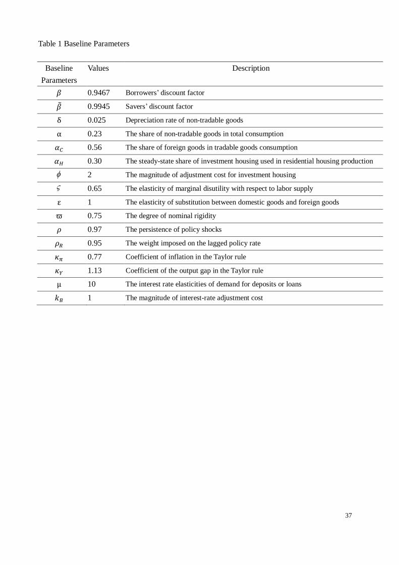
�̅� is set to be 0.6. All steady-state prices, CP , DP , Q , H , O , and S , are set to be 1. The

work hours BN and

SN are parameterized to 0.33. Table 1 summarizes the baseline

parameters and table 2 presents the steady-state values of the variables.

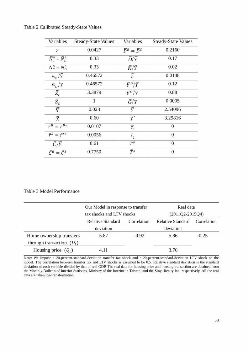
Table 3 presents our model’s relative standard deviations of housing prices and housing

transactions to output in response to transfer tax shocks and LTV shocks, which are compared

with those in the real data during 2011Q1-2015Q4. With respect to real data, housing

transactions of ownership transfer are calculated by the percentage change from the previous

period. Housing prices are measured by the percentage change from the base year’s (2011)

price. The results show that our model in response to transfer tax shocks and LTV shocks

matches the volatility of housing prices and housing transactions during the period when LTV

reduction was launched and a transfer tax was collected. One poor dimension is that our model

predicts a strongly negative correlation while real data indicates a mildly negative correlation

between housing prices and housing transactions. This may be because housing price is not the

only determinant for Taiwanese households to buy or sell residential properties. There are

other motives for engaging in housing activities, such as precautionary savings and

intergenerational transfers. Our model does not consider these factors and thus overstates the

negative correlation between housing prices and housing transactions.

4.2 Impulse Reponses

Figures 3 and 4 depict the dynamics of major variables in response to

29

20-percent-standard-deviation shocks of the residential property tax and the transfer tax. The

results indicate that an increase in the property tax rate or transfer tax rate reduces borrowers’

residential housing consumption (𝑑𝑡𝐵 ), savers’ residential housing consumption (𝑑𝑡

𝑆) and

residential housing prices (𝑞𝑡). Transfer tax shocks have a more substantially adverse impact

on residential housing prices than property tax shocks. A transfer tax depresses investment

housing price (ℎ𝑡), but not investment housing transaction (𝑘𝑡). This is because a transfer tax

is imposed on the sale of previous-period investment housing stock. The purchase of

additional investment housing in the current period greatly depends on speculators’ prospects

toward the future. If speculators foresee climbing housing prices and higher demand for

residential housing, they will purchase investment housing and hold down for residential

housing production. A property tax, relatively, increases the cost of holding properties so as to

discourage savers’ and borrowers’ residential housing consumption and speculator’s purchase

intent for investment housing. Meanwhile, greater demand for tradable consumption incites

tradable inflation, non-traded inflation and the price of investment housing.

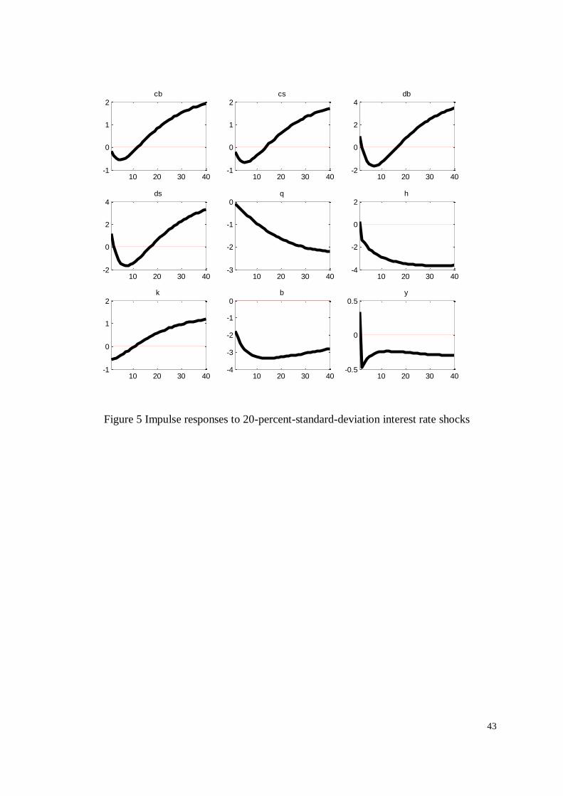
Figure 5 indicates that an increase in the policy rate reduces investment housing stock (𝑘𝑡)

and borrowing availability (𝑏𝑡). The substitution effects caused by an increase in the interest

rate dominate the income effects, reducing both savers’ and borrowers’ current tradable

consumption. To sustain higher future tradable consumption, savers and borrowers increase

their work hours, resulting in greater total production. An interest rate hike allocates

30

households’ resources from tradable consumption to housing consumption. The strengthened

current demand for residential housing initially upholds the investment housing price (ℎ𝑡).

However, an increase in the policy rate raises borrowing costs and discourages speculators

from purchasing investment housing (𝑘𝑡). Residential housing prices and investment housing

prices gradually fall. As figure 6 shows, a lower LTV ratio reduces residential housing prices

and investment housing prices. LTV shocks directly impact speculators’ borrowing capacity so

as to decrease their current residential housing consumption. Savers, by contrast, experience

increases both in tradable consumption and residential housing consumption. Higher future

demand for residential housing sustains current investment housing stock and future

investment housing prices. For most variables, LTV shocks generate similar dynamics with

transfer tax shocks.

In summary, all the policies dampen residential housing prices, but have different impact

on investment housing prices and transactions. Property tax imposition or interest rate hikes

reduces the stock of investment housing and extends the decline of investment housing prices.

Investment housing prices do not bounce back until after 40 quarters. Transfer tax imposition

or LTV ratio reduction curbs investment housing prices, but not investment housing

transactions.

Among the shocks, the borrowing availability increases rather than decreases in response

to property tax shocks. The borrowing availability is tied to the value of the multiplier of

31

collateral constraint. In equation (8), a property tax raises the ratio of current tradable

consumption over next-period tradable consumption multiplied by the ratio of the lending rate

over tradable inflation. The value of the multiplier of collateral constraint accordingly falls,

resulting in a loosened collateral constraint (more borrowing capacity). Yet, rising holding cost

of property weakens residential housing demand and gradually reduces investment housing

prices and speculators’ funding availability.

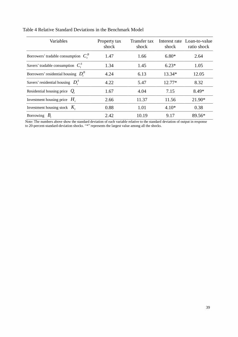
We compare the relative standard deviations under four macroeconomic policy shocks.

Table 4 indicates that interest rate shocks cause the greatest volatility of savers’ and borrowers’

tradable and housing consumption. Borrowing availability and investment housing prices

fluctuate most widely in response to LTV shocks since changes in LTV ratios affect borrowers’

funding liquidity and willingness to invest in speculative properties. Interest rate shocks and

LTV shocks generate roughly the same volatility in residential housing prices.

4.3 Sensitivity Analysis

We conduct three sensitivity analyses for the benchmark model. The first sensitivity

analysis discusses the effects of raising interest rate elasticity of demand for loans, 𝜇. A

greater 𝜇 increases the substitutability among banks, resulting in a more competitive financial

market. Figure 7 presents the impulse responses of major variables against contractionary

monetary policy shocks when 𝜇 increases from 10 to 20. After shocks occur, lending rates

(𝑟𝑡𝐵) increase but do not show significant variation in a more competitive banking

32

environment. Given the same lending rate across banks, greater bank competition fosters more

funding sources for borrowers, which mitigates the initial and sequential negative responses of

borrowing (𝑏𝑡) and the value of collateral constraint multiplier (𝛾𝑡). The investment housing

stock (𝑘𝑡) does not change significantly, however, more funding sources fuel the investment

housing price (ℎ𝑡). In a more competitive banking environment, a higher policy rate tampers

residential and investment housing prices gradually and to a lesser extent.

The second and third sensitivity analyses explore the impact of increasing the proportion

of investment housing in the residential housing production, 𝛼𝐻, from 0.30 to 0.70. As shown

in figure 8, when residential housing production relies more heavily on investment housing

than on labor, raising policy rates magnifies the decline in residential housing prices (𝑞𝑡).

Investment housing prices fall but bounce back earlier compared to the benchmark case. This

is because an interest rate hike advances the intra-temporal allocation between current tradable

goods and residential housing when the proportion of investment housing in the residential

housing production increases. Stronger demand for residential housing weakens the

effectiveness of a contractionary policy on dampening speculative housing prices and

transactions. Figure 9 shows that compared to the benchmark model, residential housing prices

decrease more and households shift consumption from residential housing to tradable goods

more substantially in response to transfer tax shocks. When the proportion of investment

housing in the residential housing production increases, speculators have greater incentives to

33

hold down unfinished housing units for future residential housing production, so the positive

initial responses of investment housing stock are stronger.

5 Conclusions

This paper evaluates the effects of several macroeconomic policies on Taiwan’s housing

market. Our results indicate that the responses of investment housing prices are closely linked

with residential housing consumption for savers and borrowers. Higher expected demand for

residential housing tends to increase speculator’s purchase intent for investment housing so as

to boost future investment housing prices. Property tax imposition and interest rate hikes

increase the holding costs of property vacancy and borrowing costs, respectively, resulting in

decreases in speculative housing transactions. They also have prolonged effects on mitigating

speculative housing prices. Transfer tax imposition and LTV ratio deduction instantly hamper

investment housing prices but not investment housing transactions. A transfer tax is imposed

on the sale of previous-period investment housing stock while a LTV shock restricts

speculators’ funding availability associated with future investment housing prices. Speculators

can potentially defer their purchase and sale decisions of speculative housing. Hence, the

impact of a transfer tax and a downward LTV ratio on moderating housing market is effective

for a limited time.

Our research has some limitations. First, the supply of investment housing is exogenously

determined. Changes in investment housing prices and stock are mainly driven by the demand

34

for residential housing. Future research can lay out a production function for investment

housing. By including land in the production function, the effects of consolidating capital

gains from transferring housing and land as taxable income can be analyzed. Second, our

research does not address the welfare comparison between different policies but focuses on the

policy impact on the housing prices and transactions. Third, we assume that all shocks occur

independently. Interrelated shocks could lead to mixed policy effects. Nevertheless, this

research builds on the channels that different macroeconomic policies draw upon the housing

market and expects to provide meaningful policy implications for the government.

35

References

1. Alpanda, S., and Zubairy, S. (2016). Housing and Tax Policy. Journal of Money, Credit

and Banking, 48, 485-512.

2. Aoki, K., Proudman, J. and Vlieghe, G. (2004). House prices, consumption, and monetary

policy: a financial accelerator approach. Journal of Financial Intermediation, 13, 414–

435.

3. Benjamin, J., Coulson, N. and Yang, S. (1993). Real estate transfer taxes and property

values: The Philadelphia story. Journal of Real Estate Finance and Economics, 7, 151–

157.

4. Besley, T., Meads, N. and Surico, P. (2014). The incidence of transaction taxes: Evidence

from a stamp duty holiday. Journal of Public Economics, 119, 61-70.

5. Best, M. and Kleven, H. (2013). Property Transaction Taxes and the Housing Market:

Evidence from Notches and Housing Stimulus in the UK. London School of Economics

Working paper.

6. Calza, A., Monacelli, T. and Stracca, L. (2013). Housing Finance and Monetary Policy.

Journal of the European Economic Association, 11, 101–122.

7. Dachis, B., Duranton, G. and Turner, M. (2012). The effects of land transfer taxes on real

estate markets: Evidence from a natural experiment in Toronto. Journal of Economic

Geography, 12, 327–354.

8. Funke, M. and Paetz, M. (2013). Housing Prices and the Business Cycle: An Empirical

Application to Hong Kong. Journal of Housing Economics, 22, 62–76.

9. Funke, M., and Paetz, M. (2016). Dynamic Stochastic General Equilibrium-based

Assessment of Nonlinear Macroprudential Policies: Evidence from Hong Kong. Pacific

Economic Review, doi: 10.1111/1468-0106.12170.

36

10. Hwang, Yu-Ning and Pei-Ying Ho (2012), “Optimal Monetary Policy for Taiwan: A

Dynamic Stochastic General Equilibrium Framework,” Academia Economic Papers, 40,

447-482.

11. Iacoviello, M. (2005). House Prices, Borrowing Constraints, and Monetary Policy in the

Business Cycle. American Economic Review, 95, 739-764.

12. Iacoviello, M. (2010). Housing in DSGE Models: Findings and New Directions. In

Housing Markets in Europe: A Macroeconomic Perspective, ed. O. de Bandt, T. Knetsch,

J. Pe˜nalosa, and F. Zollino, 3–16. Berlin, Hidelberg: Springer-Verlag.

13. Iacoviello, M. and Neri, S. (2010). Housing market spillovers: Evidence from an

estimated DSGE model. American Economic Journal: Macroeconomics, 2, 125-64.

14. Kopczuk, W. and Munroe, D. (2015). Mansion Tax: The Effect of Transfer Taxes on the

Residential Real Estate Market. American Economic Journal: Economic Policy, 7,

214-257.

15. Monacelli, T. (2009). New Keynesian Models, Durable Goods, and Collateral Constraints.

Journal of Monetary Economics, 56, 242-254.

16. Piazzesi, M. and Schneider, M. (2016). Housing and Macroeconomics, Elsevier,

Handbook of Macroeconomics, John B. Taylor and Harald Uhlig (eds.), Vol. 2.

17. Sterk, V. (2015). Home equity, mobility, and macroeconomic fluctuations. Journal of

Monetary Economics, 74, 16-32.

18. Teo, W. L. (2009), “Estimated Dynamic Stochastic General Equilibrium Model of the

Taiwanese Economy,” Pacific Economic Review, 14, 194–231.

37

Table 1 Baseline Parameters

Baseline

Parameters

Values Description

𝛽 0.9467 Borrowers’ discount factor

�̃� 0.9945 Savers’ discount factor

δ 0.025 Depreciation rate of non-tradable goods

α 0.23 The share of non-tradable goods in total consumption

𝛼𝐶 0.56 The share of foreign goods in tradable goods consumption

𝛼𝐻 0.30 The steady-state share of investment housing used in residential housing production

2 The magnitude of adjustment cost for investment housing

0.65 The elasticity of marginal disutility with respect to labor supply

ε 1 The elasticity of substitution between domestic goods and foreign goods

ϖ 0.75 The degree of nominal rigidity

𝜌 0.97 The persistence of policy shocks

𝜌𝑅 0.95 The weight imposed on the lagged policy rate

𝜅𝜋 0.77 Coefficient of inflation in the Taylor rule

𝜅𝑌 1.13 Coefficient of the output gap in the Taylor rule

μ 10 The interest rate elasticities of demand for deposits or loans

𝑘𝐵 1 The magnitude of interest-rate adjustment cost

38

Table 2 Calibrated Steady-State Values

Table 3 Model Performance

Our Model in response to transfer

tax shocks and LTV shocks

Real data

(2011Q2-2015Q4)

Relative Standard

deviation

Correlation Relative Standard

deviation

Correlation

Home ownership transfers

through transaction (𝐷𝑡)

5.87 -0.92 5.86 -0.25

Housing price (𝑄𝑡) 4.11 3.76

Note: We impose a 20-percent-standard-deviation transfer tax shock and a 20-percent-standard-deviation LTV shock on the model. The correlation between transfer tax and LTV shocks is assumed to be 0.5. Relative standard deviation is the standard

deviation of each variable divided by that of real GDP. The real data for housing price and housing transaction are obtained from the Monthly Bulletin of Interior Statistics, Ministry of the Interior in Taiwan, and the Sinyi Realty Inc, respectively. All the real data are taken log-transformation.

Variables Steady-State Values Variables Steady-State Values

0.0427 �̅�𝐵 = �̅�𝑆 0.2160

B B

C DN N 0.33 D Y 0.17

S S

C DN N 0.33 K Y 0.02

Cw Y 0.46572 b 0.0148

Dw Y 0.46572 DY Y 0.12

CZ 3.3879 CY Y 0.88

DZ 1 G Y 0.0005

0.023 Y 2.54096

χ̅ 0.60 *Y 3.29816

�̅�𝐵 = �̅�𝐵∗ 0.0107 1 0

�̅�𝑆 = �̅�𝑆∗ 0.0056 2 0

C Y 0.61 �̅�𝐵 0

𝐶̅𝐵 = 𝐶̅𝑆 0.7750 �̅�𝑆 0

39

Table 4 Relative Standard Deviations in the Benchmark Model

Variables

Property tax

shock

Transfer tax

shock

Interest rate

shock

Loan-to-value

ratio shock

Borrowers’ tradable consumption B

tC 1.47 1.66 6.80* 2.64

Savers’ tradable consumption S

tC 1.34 1.45 6.23* 1.05

Borrowers’ residential housing B

tD 4.24 6.13 13.34* 12.05

Savers’ residential housing S

tD 4.22 5.47 12.77* 8.32

Residential housing price tQ 1.67 4.04 7.15 8.49*

Investment housing price tH 2.66 11.37 11.56 21.90*

Investment housing stock tK 0.88 1.01 4.10* 0.38

Borrowing tB 2.42 10.19 9.17 89.56* Note: The numbers above show the standard deviation of each variable relative to the standard deviation of output in response to 20-percent-standard-deviation shocks. “*” represents the largest value among all the shocks.

40

Figure 1 Number of Home Ownership Transfers during 2005Q1-2016Q2

Figure 2 Sinyi Housing Price Index in Taipei City, New Taipei City and Taiwan during 2005Q1-2016Q2

41

10 20 30 40-0.02

0

0.02

0.04cb

10 20 30 40-0.02

0

0.02

0.04cs

10 20 30 40-0.2

-0.15

-0.1

-0.05

0db

10 20 30 40-0.2

-0.15

-0.1

-0.05

0ds

10 20 30 40-0.04

-0.03

-0.02

-0.01

0q

10 20 30 40-0.1

-0.05

0

0.05

0.1h

10 20 30 40-0.04

-0.02

0

0.02k

10 20 30 40-0.06

-0.04

-0.02

0

0.02b

10 20 30 400

0.02

0.04

0.06y

Figure 3 Impulse responses to 20-percent-standard-deviation property tax shocks

42

Figure 4 Impulse responses to 20-percent-standard-deviation transfer tax shocks

10 20 30 40-0.2

0

0.2

0.4

0.6cb

10 20 30 40-0.1

0

0.1

0.2

0.3cs

10 20 30 40-1

-0.5

0

0.5

1db

10 20 30 40-1

-0.5

0

0.5

1ds

10 20 30 40-0.8

-0.6

-0.4

-0.2

0q

10 20 30 40-3

-2

-1

0h

10 20 30 40-0.1

0

0.1

0.2

0.3k

10 20 30 40-2

-1.5

-1

-0.5

0b

10 20 30 40-0.3

-0.2

-0.1

0

0.1y

43

Figure 5 Impulse responses to 20-percent-standard-deviation interest rate shocks

10 20 30 40-1

0

1

2cb

10 20 30 40-1

0

1

2cs

10 20 30 40-2

0

2

4db

10 20 30 40-2

0

2

4ds

10 20 30 40-3

-2

-1

0q

10 20 30 40-4

-2

0

2h

10 20 30 40-1

0

1

2k

10 20 30 40-4

-3

-2

-1

0b

10 20 30 40-0.5

0

0.5y

44

Figure 6 Impulse responses to 20-percent-standard-deviation loan-to-value shocks

10 20 30 400

0.005

0.01

0.015cb

10 20 30 40-5

0

5

10x 10

-3 cs

10 20 30 40-0.02

0

0.02

0.04db

10 20 30 400

0.005

0.01

0.015

0.02ds

10 20 30 40-0.02

-0.015

-0.01

-0.005

0q

10 20 30 40-0.08

-0.06

-0.04

-0.02

0h

10 20 30 40-2

0

2

4x 10

-3 k

10 20 30 40-0.4

-0.3

-0.2

-0.1

0b

10 20 30 40-5

0

5

10x 10

-3 y

45

Figure 7 An increase in the interest rate elasticity of demand for loan against

20-percent-standard-deviation interest rate shocks. The dashed line represents the case when

μ = 20 and the solid line represents the case when μ = 10 (the benchmark model).

10 20 30 40-2

0

2

4db

10 20 30 40-2

0

2

4ds

10 20 30 40-3

-2

-1

0

1q

10 20 30 40-4

-2

0

2h

10 20 30 40-1

0

1

2k

10 20 30 40-4

-3

-2

-1

0b

10 20 30 40-15

-10

-5

0

5gamma

10 20 30 400

1

2

3

4rb

10 20 30 40-0.5

0

0.5y

46

Figure 8 An increase in the portion of investment housing used in residential housing

production against 20-percent-standard-deviation interest rate shocks. The dashed line represents

the case when α𝐻 = 0.70 and the solid line represents the case when α𝐻 = 0.30 (the benchmark model).

10 20 30 40-1

0

1

2cb

10 20 30 40-1

0

1

2cs

10 20 30 40-5

0

5

10db

10 20 30 40-5

0

5

10ds

10 20 30 40-8

-6

-4

-2

0q

10 20 30 40-4

-2

0

2h

10 20 30 40-1

0

1

2k

10 20 30 40-4

-3

-2

-1

0b

10 20 30 40-1.5

-1

-0.5

0

0.5y

47

Figure 9 An increase in the portion of investment housing used in residential housing

production against 20-percent-standard-deviation transfer tax shocks. The dashed line represents

the case when α𝐻 = 0.70 and the solid line represents the case when α𝐻 = 0.30 (the benchmark model).

10 20 30 40-0.5

0

0.5

1

1.5cb

10 20 30 40-0.5

0

0.5

1

1.5cs

10 20 30 40-2

0

2

4db

10 20 30 40-2

0

2

4ds

10 20 30 40-3

-2

-1

0q

10 20 30 40-3

-2

-1

0h

10 20 30 40-0.2

0

0.2

0.4

0.6k

10 20 30 40-2

-1.5

-1

-0.5

0b

10 20 30 40-0.6

-0.4

-0.2

0

0.2y