macroeconomic impacts and development outcomes for low

Macroeconomic Impacts and Development Outcomes for Low Income Countries: First Exploration of Macroeconomic Links to

Ethiopia and Ghana Distribution and Poverty Models

Background Paper Prepared for Thirteenth Annual GTAP Conference

June 2010

Penang, Malaysia

David Evans

Sussex European Institute,

University of Sussex, UK

Draft: June 2010

2

Contents Summary ......................................................................................................................................... 4

1. Background to the Research ........................................................................................................ 6

2. Available Building Blocks for the new research on Macroeconomic Impacts and Development

Outcomes ......................................................................................................................................... 7

2.1 IMF macroeconomic models ....................................................................................... 7

2.2 Case Study or “Rapid Appraisal” Methods for macroeconomic impact analysis ....... 7

2.3 Structural Models of income distribution and poverty outcomes ................................ 8

2.4 “Rapid Appraisal” of income distribution and poverty outcomes ............................... 8

3. Soft linking the available estimates of policy induced macroeconomic change to income

distribution and poverty outcomes .................................................................................................. 8

4. The First Steps ............................................................................................................................. 9

4.1 Ethiopia: Macroeconomic Scenarios .......................................................................... 9

Table 1: IMF Medium Term Projections: 2006-7 to 2012-13 ................................ 11

4.2 The SAM Database for Ethiopia ................................................................................ 12

Table 2: Economic Structure Ethiopia .................................................................... 13

4.3 The Distribution and Poverty Model ......................................................................... 14

Table 3: Macro and Factor Market Closure ............................................................ 15

4.4 Linking the Macroeconomic Projections to the Distribution and Poverty Model for

Ethiopia ............................................................................................................................ 16

Table 4a: IMF Baseline and Alternative Simulations Excluding PSURGE ........... 18

Table 4b: PSURGE for Simulations ....................................................................... 18

4.5 Ethiopia Results ......................................................................................................... 19

5. Concluding Remarks ................................................................................................................. 22

Appendix: Results Tables.............................................................................................................. 23

3

Table R1.A: Baseline and Alternative – Major Economy-wide Indicators in the Short

Run .......................................................................................................................... 23

Table R1.B: Price Surge – Major Economy-wide Indicators in the Short Run ..... 24

Table R1.C: Baseline and Alternative – Major Economy-wide Indicators in the

Medium Run ........................................................................................................... 25

Table R2.A: Baseline and Alternative – Consumption by Household in the Short Run

................................................................................................................................ 26

Table R2.B: Price Surge – Consumption by Household in the Short Run ........... 27

Table R2.C: Price Surge – Consumption by Household in the Short Run ........... 28

Table R3.A: Baseline and Alternative – Equivalent Variation by Household in the

Short Run ................................................................................................................ 29

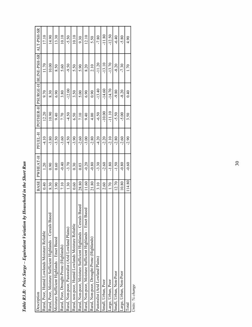
Table R3.B: Price Surge – Equivalent Variation by Household in the Short Run 30

Table R3.C: Baseline and Alternative – Equivalent Variation by Household in the

Medium Run ........................................................................................................... 31

Table R4.A: Baseline and Alternative – Savings by Institutions Including Households

in the Short Run ...................................................................................................... 32

Table R4.B: Price Surge – Savings by Institutions Including Households in the Short

Run .......................................................................................................................... 33

Table R4.C: Baseline and Alternative – Savings by Institutions Including Households

in the Medium Run ................................................................................................. 34

Table R5.A: Baseline and Alternative – Savings Shares by Institutions Including

Households in the Short Run .................................................................................. 35

Table R5.B: Price Surge – Savings Shares by Institutions Including Households in the

Short Run ................................................................................................................ 36

Table R5.C: Baseline and Alternative – Savings Shares by Institutions Including

Households in the Medium Run ............................................................................. 37

References ..................................................................................................................................... 38

4

Summary This strategic draft of a paper first outlines a new area of policy orientated research on the

Macroeconomic Impact on LIC Development Outcomes. The initial pilot research uses IMF

macroeconomic policy, an area of research that has challenged policy makers within the IMF and

within the development community for a long time. The preliminary results for Ethiopia of a

“soft link” from macroeconomic scenarios presented in an IMF Article IV report to a recent

general equilibrium comparative static CGE model of distribution and poverty are reported.

There are four key ideas in this project, to be applied initially to African LIC countries:

1. To “soft link” currently available IMF macroeconomic models to available income

distribution and poverty models to provide estimates of poverty outcomes of IMF

endorsed macroeconomic policies;

2. Where macroeconomic models are unavailable, to upgrade the quality of the

macroeconomic “rapid appraisal” case studies built around IMF Letters of Intent and

Article IV reports, so that macroeconomic scenarios can be soft linked to income

distribution and poverty models;

3. Where the database for income distribution and poverty models is not available, develop

a “rapid appraisal” approach to estimating income distribution and poverty impacts using

a wide range of readily available structural and poverty indicators (See below “rapid

appraisal”); and

4. Should the structural data assembled under 3 be sufficiently comprehensive to consider

building small-to medium-sized SAMs that can be used to build structural income

distribution and poverty models as in 1.

The macroeconomic scenarios suggested for Ethiopia in the 2009 Article IV report were

principally designed to lower the level of domestic inflation and to offset the effects of the boom

in world food and oil prices by limiting the increase in the fiscal balance in the short and medium

Run, and by increasing access to foreign savings through the IMF. The real outcomes of the

anti-inflationary policies in the Article IV scenarios were applied to the CGE model. The

principal driver of the first distribution and poverty results for Ethiopia was the increase in

foreign savings which produced an appreciation of the real exchange rate in the short and

medium Run and an increase in welfare for rural as opposed to urban households. So far, a

5

consistent measure of the strength of the world price surge could not be found. IMF assistance to

obtain an appropriate measure of the world price surge will be sought for the final version of the

paper. Revised results for Ethiopia and comparative static results for Ghana should be available

by the end of April.

6

1. Background to the Research

Policy-orientated research on the Macroeconomic Impact on LIC Development Outcomes has

challenged policy makers within the IMF and within the development community for a long

time. The results so far have been unsatisfactory. This project aims to fill a major gap with first

examples from IMF macroeconomic policies.

This project has for key purposes, to be applied first to African LIC countries:

1. To “soft link” currently available IMF macroeconomic models to available income

distribution and poverty models to provide estimates of poverty outcomes of IMF

endorsed macroeconomic policies. The term “soft link” is from the climate modelling

literature. It means an informal linking of models through the exogenous variables, rather

than a formal linking of the models themselves. It is anticipated that the structural models

of income distribution and poverty will be much more aggregated on the sectoral side

than normally used for poverty analysis, but not factors or households.

2. Where macroeconomic models are unavailable, to upgrade the quality of the

macroeconomic “rapid appraisal” case studies built around IMF Letters of Intent and

Article IV reports so that macroeconomic scenarios can be soft linked to income

distribution and poverty models. (See below on “rapid appraisal”). The IMF research

department has offered assistance in gaining initial experience with their macroeconomic

case studies. Only later in the main project will more independent macroeconomic

scenarios be considered.

3. Where the database for income distribution and poverty models is not available, develop

a “rapid appraisal” approach to estimating income distribution and poverty impacts using

a wide range of readily available structural and poverty indicators (See below on “rapid

appraisal”).

4. Should the structural data assembled under 3 be sufficiently comprehensive,

consideration will be given to building small to medium sized SAMs that can be used to

build structural income distribution and poverty model as in 1. Should we be successful

in building such intermediate sized SAMs with modest sectoral treatment but more

7

disaggregated factor and household data, we would not expect the same degree of

comprehensiveness or accuracy as for a full-sized SAM.

The key background idea to the project is applying “rapid appraisal” methodologies to fill the

gaps in modelling availability. The idea is to develop a set of readily available macroeconomic

data and a set of structural data on distribution and poverty which, when combined with rules of

thumb from economic theory, can be used to inform a qualitative analysis of macroeconomic

policy impacts and distribution and poverty outcomes. The idea behind such “rapid appraisal”

analyses comes from the Sussex Method for the assessment of regional integration schemes (see

the original DfID report Evans et al 2006)).

2. Available Building Blocks for the new research on Macroeconomic Impacts and Development Outcomes

2.1 IMF macroeconomic models

At present, the Fund has well-developed Dynamic Stochastic General Equilibrium (DSGE)

macroeconomic models for only a few African LICs (see Berg et al., 2006). However, the real

side of these models is unsuitable for income distribution and poverty impact analysis. The same

is true of other macroeconomic models such as the IMMPA suite of models (see Agenor, 2007).

Hence the idea is to soft link available DSGE models to structural models of distribution and

poverty, as described in 2.3 below, and to develop “rapid appraisal” methodologies for 2.2 and

2.4.

2.2 Case Study or “Rapid Appraisal” Methods for macroeconomic impact

analysis

At present, macroeconomic case studies are widely available through Letters of Intent and

Article IV reports but are of variable quality. Where possible, they will be used for estimating

macroeconomic impact soft links to income distribution and poverty outcome analysis as

described in 2.3 below. Where available IMF case studies are weak, consideration will be given

to develop them using a more systematic “rapid appraisal” methodology.

8

2.3 Structural Models of income distribution and poverty outcomes

There is a large literature on Computable General Equilibrium modelling of income distribution

and poverty impacts of economic policy change (see for example Bourguignon, 2008). For some

of these countries, there are SAMs suitable for Running dynamic recursive income distribution

and poverty models. The DSGE macroeconomic models from 2.1 or the macroeconomic impact

analysis from the “rapid appraisal” methods in 2.2 can be used to quantify key exogenous macro

variables under baseline and other scenarios for the structural models of distribution and poverty

such as: government and investment expenditure; private, government and foreign savings; and

choice of other policies and instruments such as transfers to households, tariffs, direct and

indirect taxes.

2.4 “Rapid Appraisal” of income distribution and poverty outcomes

Among the African LICs countries, there are large gaps in coverage of SAMs suitable for

modelling income distribution and poverty impacts of macroeconomic policies. In these cases,

the idea is to develop a “rapid appraisal” approach to estimating income distribution and poverty

impacts using a wide range of readily available indicators. The key ideas for such a “Rapid

Appraisal” approach can be found in technical reports of structural CGE models, where summary

structural data from the underlying SAM is usually reported and used for a preliminary impact

analysis of model shocks. (The Handbook of Trade and Poverty, Cirera et al., 2001) Where

possible, such datasets will be upgraded to small-to medium-sized SAMs for formal structural

and distribution and poverty analysis.

3. Soft linking the available estimates of policy induced macroeconomic change to income distribution and poverty outcomes The heart of the concept note is in preparation for a programme of research over 2 years on how

to soft link either formal or informal macroeconomic impact estimates to generate the formal or

informal structural and income distribution outcome estimates from the Building Blocks

described in 2.1 to 2.4 above, and on how to strengthen the rapid appraisal components in 2.2

and 2.4. The first step in this programme is to develop soft links between the estimates of key

macroeconomic impacts to income distribution and poverty outcomes, that is, to soft link

9

macroeconomic impacts from 2.1 or 2.2 to distribution and poverty outcomes estimated by

formal structural income distribution models as in 2.3. In the process, it is anticipated that the

rapid appraisal components, 2.2 and 2.4, will be upgraded and attempts will be made to soft link

formal or informal macroeconomic impact estimates as in 2.1 or 2.2 to the informal estimates of

income distribution and poverty outcomes as in 2.4.

The key to the above research programme is to make operational the soft links set out in section

3, starting with soft links between 2.1 and 2.3, and between and 2.2 and 2.3. For this purpose,

two pilot countries have been chosen, Ethiopia and Ghana. Both pilot countries have large recent

SAMs and Running income distribution and poverty models. The IMF has a DSGE model for

Ghana, but has only used case study methods to estimate macroeconomic impacts for Ethiopia.

In terms of the building blocks described, for Ghana the soft linkages will be based on the formal

macroeconomic model as in 2.1 to a formal structural income distribution and poverty outcome

model as in 2.3. For Ethiopia informal macroeconomic impacts estimated as in 2.2 will be soft

linked to a structural income distributing and poverty outcome model as in 2.3. In this draft

paper, only the Ethiopia results have been reported.

4. The First Steps

4.1 Ethiopia: Macroeconomic Scenarios

The account of Ethiopian macroeconomic policies reported here is based on IMF Country Report

No 08/264 July 2008. It turned out that the soft links from the 2008 IMF Macroeconomic

Projections for Ethiopia were quite straightforward. Clearly the projections are dated, but

combined with the distribution and poverty model based on the 2005-6 Ethiopia SAM (Robinson

et al 2010), it is possible to conduct an ex post feasibility experiment estimating the distribution

and poverty impact of the macroeconomic projections in the IMF 2008 Ethiopia Country Report.

In 2008, the Ethiopian policy context was driven primarily by strong pro-growth development

policies from 2003/4 consistent with poverty reduction, high domestic inflation and a world food

and oil price “surge”. More recently, it became clear that demand was running ahead of the

expansion in the capacity of the economy and international reserves had fallen to about 1.5

months of imports. The IMF argued that inflation was being led by rapidly rising food prices;

10

rising global prices were also playing a role but the mechanism was not clear. The surge in world

oil prices placed further strain on Ethiopia’s balance of payments.

The Ethiopian policy response was to address the macroeconomic imbalances as well as to

absorb the severe world oil price shock in a manner that would least affect the momentum for

growth and poverty reduction. They planned to reduce broad money growth to under 20 percent

and support lower monetary growth by implementing a cautious fiscal policy that kept domestic

borrowing well within the budget ceiling. IMF staff urged forceful measures to prevent inflation

expectations from becoming ingrained and to strengthen the balance of payments.

The policy response to the macroeconomic situation as it emerged in 2008 is summarized in the

projections from IMF (2008, p12), shown in Table 1 below.

11

Table 1: IMF Medium Term Projections: 2006-7 to 2012-13

% GDP unless otherwise stated

2006-7 2007-8 2008-9 2009-10 2010-11 2011-12 2012-13

Baseline Actual Projection Projection Projection Projection Projection Projection Real GDP growth (annual % Change)

11.4 8.4 6 6.5 7 7.5 7.5

Fiscal Balance (including grants)

-3.1 -4.4 -3.5 -3.7 -3.4 -3.4 -3.7

Current Account Balance (including grants)

-4.5 -4.8 -6.2 -6.1 -6.6 -5.7 -5

% GDP unless otherwise stated

2006-7 2007-8 2008-9 2009-10 2010-11 2011-12 2012-13

Alternative Actual Projection Projection Projection Projection Projection Projection Real GDP growth 11.4 8.4 7 7.5 8 8 8 Growth TFP relative to Baseline

0.00 0.00 1.00 1.00 1.00 0.50 0.50

Fiscal Balance (including grants)

-3.1 -4.4 -3.5 -3.7 -3.7 -3.7 -3.8

Current Account Balance (including grants)

-4.5 -4.8 -7.6 -7.3 -6.9 -5.7 -4.9

Source: Table 1 From IMF Country Report No 08/264 July 2008 p12.

Table 1 shows two sets of projections of the Fiscal Balance and Current Account Balance from

the base year 2006-7 to 2012-13. Over the six-year projection period from 2006-7, the Baseline

scenario allows a further decrease in the fiscal deficit, followed by a return in the final period to

a level closer to the initial base level for 2006/7. In other words, the short-Run fiscal deficit was

to increase in the adjustment transition before being reined in by macroeconomic policy

measures by the final period of the projection. The current account deficit in the Baseline

scenario also increases sharply, and is then reduced to a level closer to the initial base period.

The profile of the Alternative scenario is very similar to the Baseline, the primary difference

being a larger increase in the fiscal and current account balances in the transition to the final

period, which has slightly higher levels in the base period. A powerful additional element enters

into the Alternative macroeconomic scenario, namely an enhanced profile of the technical

change or TFP improvement relative to the Baseline. The TFP effect is largely assumed to result

from a range of policy measures assumed to complement the Alternative macroeconomic

scenario such as additional grants for public spending, some of which would be allocated for

12

capital projects that have high import content and raise longer-term growth. Short-term growth is

also higher than in the Baseline because finance for imports helps alleviate shortages of key

commodities.

4.2 The SAM Database for Ethiopia

The 2006 SAM used in the distribution and poverty model general equilibrium or CGE model

for Ethiopia is described in Ahmad et al (2010). It is highly disaggregated allowing for a large

model with 50 activities, 22 commodities, 15 factors and 15 households. Agricultural activities

are divided by region as are two factors, land and livestock. Only two out of five types of labour

are mobile across activities and regions and capital is used only in manufacturing activities.

There are 10 rural and 5 urban households, and foreign trade is divided by regions of origin and

destination. Using the SAM, a brief summary of the economic structure of Ethiopia is shown in

Table 2 below.

13

Table 2: Economic Structure Ethiopia

Description Share Share Share Share Share Share Share

Dom. Total Total Exports Imports HH Rural Poor

Prod. Imports Exports Output D.Dem. Cons. Cons.

Teff 0.01 0 0 0 0 0.02 0.01

Wheat 0.01 0.04 0 0 0.49 0.02 0.04

Maize 0.01 0 0 0 0 0.01 0.02

Barley and sorghum 0.01 0 0 0 0 0.01 0.02

Export agriculture 0.04 0 0.34 0.73 0.02 0.03 0.03

Enset 0 0 0 0 0 0.01 0.01

Other agricultural products 0.04 0.01 0.04 0.11 0.08 0.06 0.06

Livestock 0.05 0 0.05 0.08 0.01 0.07 0.05

Home-produced agricultural products 0.12 0 0 0 0 0.2 0.29

Total Agriculture 0.29 0.05 0.43 0.43 0.53

Home-produced processed food, services 0.09 0 0 0 0 0.14 0.2

Flour and milling services 0.01 0 0.02 0.17 0.07 0.01 0.01

Other processed food, beverages, tobacco 0.03 0.03 0.03 0.1 0.23 0.06 0.04

Chemicals 0.01 0.12 0.02 0.2 0.82 0.04 0.04

Electricity 0.01 0 0 0 0 0.01 0

Water 0.01 0 0 0.05 0 0 0

Petrol 0 0.12 0 - 1 0.01 0.01

Intermediate and investment goods 0.02 0.09 0.03 0.15 0.57 0.01 0.01

Final consumer goods 0.03 0.34 0.07 0.2 0.78 0.12 0.07

Total Manufactured Goods 0.21 0.7 0.17 0.4 0.38

Construction services 0.11 0 0 0 0 0 0

Trade and transport services 0.18 0.17 0.3 0.14 0.22 0.03 0.01

Public admin, education, health services 0.11 0 0.01 0.01 0 0.03 0.02

Other services 0.1 0.07 0.1 0.09 0.02 0.12 0.08

Total Construction and Other Services 0.5 0.24 0.41 0.18 0.11

Total 1 1 1 1 1

Source: 2005-6 Ethiopia SAM

The structure of the Ethiopian economy follows a pattern of imports, exports, domestic

production, and consumption that is familiar for low income developing countries. For trade, on

the import side, agricultural products were about 5% for 2005/6 made up almost entirely of

Wheat. Other large items imported include Chemicals, Petrol, Intermediate and Investment

goods, Final Consumer Goods and Transport Services. One the export side, Export Agriculture

(for example coffee) and Trade and Transportation Services are the largest items. Note that

14

Home-produced agricultural products, largely non-traded goods, form 12% of estimated

domestic production.

The large degree of sector and regional disaggregation in the SAM is likely to ensure that the

poverty and distribution impact results for macroeconomic scenarios are as large as possible. In

later refinement of the work, regional, activity and commodity aggregations will be used to see

how far the distribution and poverty results are affected by aggregation.

4.3 The Distribution and Poverty Model

The distribution and poverty general equilibrium model or CGE model for Ethiopia described in

Appendix 2 used in this research is comparative static (see Robinson et al 2010. The key

modelling assumptions are:

• Value added is modelled using constant elasticity of substitution (CES) production

functions for factor inputs (land, livestock capital, various types of labour and non-

agricultural capital).

• Intermediate inputs into production are determined as fixed shares of the quantity of

output.

• Payments from each factor of production are allocated to households and other

institutions using fixed shares derived from the base SAM.

• Household consumption is modelled using a Linear Expenditure System (LES)

specification. Imported goods are assumed to be imperfect substitutes for domestically

produced goods.

• Exported goods are imperfect substitutes for domestically produced and consumed goods.

• The domestic price of each commodity adjusts so that domestic supply equals domestic

demand.

• Capital stock (including livestock capital) is fixed in each sector and region. Land is fixed

by region, and is allocated across crops so that the value of the marginal return to land is

equal across each crop in a given region.

15

• Labour markets have the total supply of labour of each skill type is fixed (and fully

employed). Real wages adjust so that demand for labour is equal to supply.

• External accounts have fixed foreign savings (foreign capital inflows). With fixed foreign

transfers, the trade balance (and fixed current account balance) are also fixed

• The real exchange rate adjusts to achieve an export supply and import demand that yield

the fixed trade balance.

• The numeraire (i.e. reference price) of the model is the consumer price index. Thus, the

model determines prices relative to this fixed CPI.

• The “macro closure” assumptions made are discussed below.

• The full set of equations for the distribution and poverty model are set out in Robinson et

al (2010, Annex 1)

The “macro closure” assumptions made are crucial for the “soft linking” of the IMF Article IV

projections for Ethiopia to the distribution and poverty model. Note that in the general

equilibrium context, macro closure refers to the choice of exogenous and endogenous variables

for saving and investment, for government, for foreign trade and for factor markets. The choices

made for the scenarios Run for Ethiopia are shown in Table 3 below.

Table 3: Macro and Factor Market Closure

Savings-Investment Fixed investment, savings endogenous Government Fixed Government Savings, government expenditure adjusts World Fixed foreign savings, real exchange rate endogenous Factor markets Fixed factor supplies, endogenous factor returns, specific capital in

manufacturing in short Run

Numeraire CPI

The choice of the macro closure provides a framework within which the macroeconomic

scenarios described above can be assessed. Investment is exogenous and the rate of savings from

private income adjusts so that investment can be financed. Government savings (or if negative,

deficit) is a key macroeconomic policy variable, so it makes sense for government savings to be

exogenous in the general equilibrium model and for government savings to be given by the

16

macroeconomic scenarios. With government savings exogenous, government expenditure is

endogenous, adjusting so that with endogenous government income, the government income and

expenditure balances are satisfied. For the rest of the world, foreign savings is a particularly

important macroeconomic variable. As noted above, when foreign savings are exogenous, the

real exchange rate in the general equilibrium model is endogenous. In summary, government

savings and foreign savings in the macroeconomic scenarios are the key endogenous policy

variables which appear in the general equilibrium model as exogenous variables as described in

Table 3 above.

Other choice of closure will be checked for sensitivity as the results develop, for example the

fixed supply of factors assumption in markets for unskilled labour. There is a considerable

debate in Ethiopia on the nature of the market for foreign exchange, but for present purpose the

real exchange rate adjusts to clear the foreign exchange market. Note that it is the real exchange

rate that is flexible, not the REER as discussed in the macroeconomic literature. Here, the real

exchange rate is the ratio of non-traded to traded goods prices as is used in the theory of

international trade when there are traded and non-traded goods. The final set of macroeconomic

scenarios used for the general equilibrium model is described in section 4.4 and in Table 4

below.

4.4 Linking the Macroeconomic Projections to the Distribution and Poverty

Model for Ethiopia

In the simulations described in Tables 4a and 4b below, the short Run is taken to be roughly 3

years, and capital, used in manufacturing only, is sector specific, compared with the medium Run

(roughly 5 years) is fully mobile within manufacturing. The description of the scenarios follows

the conventions:

Across the column headings:

GAVSIM is government savings by scenario

FSAVSIM is foreign savings by scenario

TFP is Total Factor Productivity change by scenario

17

World Price is the change in the price of exports and imports used in the model

by scenario

Across the row headings, the scenario names are composites base on

BLINE is Baseline

ALT is Alternative

G is Government Savings

F is Foreign Savings

PWHEAT etc are world prices of exports and imports

H refers to “high” world price change for exports and imports

L refers to “low” world price change for exports and imports

SR short Run, roughly 3 years

MR medium Run, roughly 6 years

Note that the BASE values for the differential rates of TFP in the Baseline and Alternative

simulations described in Table 1 are assumed to be cumulative.

18

Table 4a: IMF Baseline and Alternative Simulations Excluding PSURGE

GSAVSIM FSAVSIM TFP World Price

No BASE % change BASE % change % change % change

1 G-BLINE-SR 3.26 -24.35 13.07 0.00 0.00 0.00

2 F-BLINE-SR 3.26 0.00 13.07 16.19 0.00 0.00

3 BLINE-SR 3.26 -24.35 13.07 16.19 0.00 0.00

4 G-ALT-SR 3.26 -24.35 13.07 0.00 0.00 0.00

5 F-ALT-SR 3.26 0.00 13.07 28.34 0.00 0.00

6 TFP-ALT-SR 3.26 0.00 13.07 0.00 2.00 0.00

7 ALT-SR 3.26 -24.35 13.07 28.34 2.00 0.00

8 PWHEAT-H 3.26 0.00 13.07 0.00 0.00 see Table 4b

9 PFUEL-H 3.26 0.00 13.07 0.00 0.00 see Table 4b

10 POTHER-H 3.26 0.00 13.07 0.00 0.00 See Table 4b

11 PSURGE-H 3.26 0.00 13.07 0.00 0.00 See Table 4b

12 BLINE-PSH-SR 3.26 -24.35 13.07 16.19 0.00 See Table 4b

13 ALT-PSH-SR 3.26 -24.35 13.07 28.34 2.00 See Table 4b

14 G-BLINE-MR 3.26 -24.35 13.07 0.00 0.00 0.00

15 F-BLINE-MR 3.26 0.00 13.07 5.06 0.00 0.00

16 BLINE-MR 3.26 -24.35 13.07 5.06 0.00 0.00

17 G-ALT-MR 3.26 -28.41 13.07 0.00 0.00 0.00

18 F-ALT-MR 3.26 0.00 13.07 4.05 0.00 0.00

19 TFP-ALT-MR 3.26 0.00 13.07 0.00 4.00 0.00

20 ALT-MR 3.26 -28.41 13.07 4.05 4.00 0.00

21 PSURGE-L 3.26 0.00 13.07 0.00 0.00 See Table 4b

22 BLINE-PSL-MR 3.26 0.00 13.07 0.00 0.00 See Table 4b

23 ALT-PSL-MR 3.26 -28.41 13.07 4.05 4.00 See Table 4b

Table 4b: PSURGE for Simulations

Commodities Export % change Import % change

PWHEAT-H 64.00 64.00

PFUEL-H - 50.00

POTHER-H

- Maize 28.00 28.00

- Barley and Sorghum 26.00 26.00

- Agricultural Exports 50.00 50.00

- Other Agriculture 50.00 50.00

- Livestock 30.00 30.00

- Food 10.00 50.00

PSURGE-L:

- 25% of PSURGE-H

19

The sources for Tables 4a and 4b are as follows: For Table 4a, The IMF estimates of the changes

in government and foreign savings in Table 1 as a % of GDP by scenario. TFP differentials

between scenarios are also shown in Table 1 and are included in Table 4a for the Alternative

scenario. In Table 4a, the Base year levels of government and foreign savings shown are from

the 2005/6 SAM (Ahmed et al (2010)). The per cent change in government and foreign savings

in Table 4a combines the implied changes in the absolute values from Table 1 with the SAM

Base year levels shown in Table 4a to get the % change in Table 4a which is used in the model.

Thus, the % changes in government and foreign savings from Table 1 were applied to the model

database so they could be used in the SAM based comparative static model. Since the critical

results from a comparative static model are in % changes, the impact effects of the IMF

scenarios in Table 1 are captured by the distribution and poverty model. Short and long Run TFP

change was estimated cumulatively for the first 3 and for 6 years in Table 1. The worksheets

from Robinson et al (2010) were used for the PSURGE export and import price change for Table

4b. Altogether, 24 simulations were calculated. They were grouped in the following way:

• Simulations 1-7 were for the short-Run with varying combinations of government and

foreign savings and TFP.

• Simulations 8-12 examine the components of the PSURGE simulations for the high

projects of world price change.

• Simulations 13-14 put together all the components of the SR simulations.

• Simulations 15-23 put together varying combinations of the MR simulations. There is

less attention given to the PSURGE simulations, partly because their impact is explored

in simulations 8-12, and partly because in the MR, the size of the PSURGE simulations is

only 25% of those in the SR.

4.5 Ethiopia Results

The results tables shown in the Appendix are disaggregated by the 23 components of the major

scenarios for the major economic variables covered: economy-wide indicators, household

20

consumption, equivalent variation by household,1 savings and savings shares by institutions

including disaggregated households. The scenarios are grouped into the short run (SR), the price

purge, and the medium run (MR) with an aggregate MR price surge. All of the results are shown

as a % change on base. Except for equivalent variation, all of the Base values are taken from the

2005/6 Ethiopia SAM. Some scenarios are disaggregated even though policy makers saw the

underlying economic rationale crossing two or more disaggregated scenarios. For example, TFP

projections are linked to additional grant funding which is included in foreign savings. A revised

set of scenarios could be constructed which included successful and unsuccessful TFP growth,

always including the additional grant funding included in foreign savings.

A first step towards understanding the results is to explore the impact of the different economic

drivers and tracing the poverty impacts. Consider the principal drivers:

• Changes in government savings

• Changes in foreign savings

• Changes in world prices or terms of trade

• Total factor productivity or TFP

From Table R1.A it can be seen that a fall in government savings (increase in debt) leads to a

large increase in government expenditure, but a small effect on all other economic indicators.

The small decline of real exchange rate (the price of domestic goods over foreign goods)

suggests a switch in expenditure between households and government from foreign to domestic

in conformity with expectations, but the economic impact is small. This result is repeated

throughout all the scenarios and indicators reported in the Appendix. This is not a comment on

the effectiveness of the macroeconomic policies behind the projections of government savings

(debt), but a reflection of the small real economic effects of the implied expenditure switching.

In contrast to the projected changes in government savings, the projected increase and then

relative decline in foreign savings has substantial economic effects. First, the increased supply of

1 Equivalent variation (EV) takes account of differences in consumer preference across households as revealed by observed spending patterns, and provides an exact money-metric measure of the change in utility due to the

exogenous shock under consideration.

21

foreign exchange leads to an appreciation of the real exchange rate, lowering exports and

increasing imports. Aggregate welfare as measured by the change in absorption (imports plus the

production of importables) increases substantially as a result of the rise in foreign savings and is

a dominant contributor to the impact effects of both the Baseline and Alternative scenarios in the

SR and in the MR, as can be seen from the results tables.

The changes in world prices through the SR price surges shown in Table R.1B and the changes

in SR TFP shown in Table R.1C are more problematic. Taking TFP first, the impact of the

projected TFP improvement in the Alternative scenario is always large, stimulating exports

compared with import competing production so that the real exchange rate depreciates. Similar

results arise for the MR, shown in Table R1.C, however, there is no hard evidence to show that

the increased grants will lead to the projected TFP changes. This SR and MR result should be

regarded as speculative. Similarly, the data used to analyse the price surge was not from the

Article IV country report, but was from a later project conducted for the World Food Programme

in Ethiopia. The data was compiled in 2009 and was not projected on the same basis as the

projections in the Article IV report. As can be seen from Table R.1.B, the SR “Price Surge

Other” result had very large terms of trade and real exchange rate effects. Without further and

much more careful analysis, this result should be discounted. The SR price surge results for

Wheat and Fuel are of greater interest. The world price increase for wheat benefits exporters

leading to a real exchange rate appreciation. On the other hand, imported wheat is consumed in

urban households leading to a negative welfare effect as indicated by the decline in the terms of

trade. In the case of fuel, there is no domestic fuel production so the rise in fuel prices leads to a

depreciation of the real exchange rate and a strong negative terms of trade effect. The negative

effects on the welfare of the fuel price increase is partly compensated for by the depreciation of

the real exchange rate which leads to a substantial increase in exports.

The poverty impacts of the four drivers discussed above can be seen in Tables R2.A-C and

Tables R3.A-C in the Appendix. Broadly speaking, the projected increases in government debt in

the SR with no substantial decline in the MR leads to a modest decrease in the consumption of

the poorest rural households. In contrast, the rise in foreign savings in the SR with only a modest

reversal of the increase in the MR leads to substantial improvements in consumption of the

poorest rural households. The SR increase in the price of wheat has mixed positive and negative

effects on the poorest rural households and on urban poor households. In contrast, the SR

22

increase in the price of fuel has strong negative consumption effects across the board especially

for the rural poor.

Tables R4.A-C also show the effects on savings of the different scenarios, the mirror image of

the key results reported. For example, the SR increase in foreign savings given government

savings leads to a sharp decline in household savings – a necessary consequence of the closure

assumptions of the model. There is a fixed amount of investment that has to be financed, and if

the foreign component increases and the government component does not change, then the

household savings decline. This is the mechanism by which households gain from the increased

foreign savings. Other closure assumptions could and should be explored in future work.

Finally, there is nothing in the model metric to analyse tradeoffs between additional current

foreign savings that allow an increase in current household consumption, and a future repayment

of the additional foreign savings and the associated cost in terms of further consumption

foregone. Future work in this area would benefit from working in a recursive dynamic context.

5. Concluding Remarks The above results for Ethiopia suggest that the soft link from the Article IV Baseline and

Alternative macroeconomic scenarios to a general equilibrium model of the distribution and

poverty is feasible and useful. The main driver of the results so far was the increase in foreign

savings leading to an appreciation of the real exchange rate, a decline in exports and an

improvement in rural relative to urban household welfare.

Much more needs to be done to flesh out the macroeconomic scenarios and the distribution and

poverty consequences for Ethiopia, particularly in relation to an analysis of how rural households

gain from the appreciation of the real exchange rate. Also, analysis is needed in relation to the

change in government expenditure. The impact of alternative factor market closure needs to be

explored and the impact of the surge in world market prices that took place over the period of

analysis and aggregation of the SAM to gain insights on the best size of SAM for the analysis. It

would be useful to repeat the analysis with a recursive dynamic version of the Ethiopia model.

Analysis of Ghana results in the comparative static context is proceeding and will be reported as

soon as possible.

23

App

endix: Results Tables

Tab

le R1.A: Baseline an

d Alte

rnative – Major Econo

my-wide Indicators in

the Sh

ort R

un

Description

BASE

G-BLINE-SRF-BLINE-SRBLINE-SR

G-ALT-SR

F-ALT-SR

TFP-ALT-SR

ALT-SR

GDP

128.60

-0.01

0.08

0.08

-0.01

0.10

2.00

2.10

Absorption

158.80

-0.01

1.40

1.40

-0.01

2.40

1.60

4.00

HH Consumption

114.80

-0.30

2.10

1.80

-0.30

3.70

2.00

5.30

Investment

28.20

Gov. Expend.

15.90

2.40

-1.20

1.30

2.40

-2.10

1.80

2.20

Exports

16.80

0.09

-6.80

-6.70

0.09

-11.60

2.80

-8.70

Imports

47.00

0.03

2.10

2.10

0.03

3.80

1.00

4.80

Real Exchange Rate

1.00

-0.30

-3.00

-3.30

-0.30

-5.30

0.60

-4.90

Terms of Trade

100.00

Invest. Share GDP

21.30

0.00

-0.50

-0.50

0.00

-0.90

-0.50

-1.40

FSAV share GDP

9.90

-0.03

1.20

1.20

-0.03

2.00

-0.10

1.90

Trade Def. share GDP

22.80

-0.08

0.80

0.70

-0.08

1.30

-0.30

0.90

Units: B

illion birr and

% cha

nge

24

Tab

le R1.B: Price Surge – M

ajor Econo


the Sh

ort R

un

Description

BASE

PWHEAT-H

PFUEL-H

POTHER-H

PSURGE-H

BLINE-PSH-SRALT-PSH-SR

GDP

128.60

-0.20

-0.20

-0.20

-0.20

-0.10

2.00

Absorption

158.80

-0.40

-1.90

2.20

0.03

1.20

3.70

HH Consumption

114.80

-0.50

-2.90

4.00

0.80

2.10

5.40

Investment

28.20

Gov. Expend.

15.90

-0.20

1.80

-6.60

-5.30

-3.20

-2.20

Exports

16.80

-3.60

8.90

5.50

9.90

4.70

3.80

Imports

47.00

-2.20

-2.80

9.80

4.20

6.10

8.60

Real Exchange Rate

1.00

-1.00

3.20

-19.00

-17.30

-19.40

-20.30

Terms of Trade

100.00

-2.50

-5.60

17.40

8.40

8.40

8.40

Invest. Share GDP

21.30

-0.20

1.70

-3.60

-2.60

-2.90

-3.60

FSAV share GDP

9.90

-0.10

0.60

-2.20

-1.90

-0.90

-0.20


22.80

-0.20

1.30

-5.10

-4.40

-3.70

-3.40

Units: B

illion birr and

% cha

nge

25

Tab

le R1.C: Baseline an

d Alte

rnative – Major Econo


the Medium Run

Description

BASE

G-BLINE-MRF-BLINE-MRBLINE-MR

G-ALT-MR

F-ALT-MR

TFP-ALT-MRALT-MR

PSURGE-L

BLINE-PSL-MRALT-PSL-MR

GDP

128.60

-0.02

0.03

0.01

-0.02

0.02

4.00

4.10

-0.01

0.00

4.00

Absorption

158.80

-0.01

0.40

0.40

-0.02

0.40

3.30

3.60

-0.10

0.20

3.50

HH Consumption

114.80

-0.60

0.60

0.06

-0.70

0.50

4.10

3.90

0.04

-0.06

3.90

Investment

28.20

Gov. Expend.

15.90

4.00

-0.30

3.80

4.70

-0.20

3.30

7.90

-1.70

2.30

6.40

Exports

16.80

-0.01

-2.30

-2.30

-0.01

-1.80

5.80

3.90

3.60

1.90

7.70

Imports

47.00

0.00

0.60

0.60

0.00

0.50

2.10

2.50

0.80

1.30

3.50

Real Exchange Rate

1.00

-0.02

-0.80

-0.80

-0.03

-0.70

0.80

0.10

-4.70

-5.40

-4.60

Terms of Trade

100.00

2.30

2.30

2.30

Invest. Share GDP

21.30

0.09

-0.10

-0.04

0.10

-0.10

-0.80

-0.80

-0.70

-0.70

-1.50

FSAV share GDP

9.90

0.01

0.40

0.40

0.01

0.30

-0.30

0.02

-0.50

-0.20

-0.50


22.80

0.02

0.30

0.30

0.03

0.20

-0.70

-0.50

-1.20

-1.00

-1.60

Units: Billion birr and % change

26

Tab


d Alte

rnative – Con

sumption by H

ouseho

ld in

the Sh

ort R

un

Description

BASE

G-BLINE-SR

F-BLINE-SR

BLINE-SR

G-ALT-SR

F-ALT-SR

TFP-ALT-SRALT-SR

Rural, Poor, Humid Lowlands Moisture Reliable

0.40

-1.40

4.60

3.20

-1.40

8.00

2.70

9.20

Rural, Poor, Moisture Sufficient Highlands – Cereals Based

8.30

-1.20

4.00

2.70

-1.20

6.90

2.60

8.20

Moisture Sufficient Highlands – Enset Based

3.90

-1.10

3.80

2.60

-1.10

6.60

2.50

7.90

Rural, Poor, Drought-Prone (Highlands)

7.10

-1.00

3.60

2.60

-1.00

6.30

2.40

7.70

Rural, Non-poor, Pastoralist (Arid Lowland Plains)

1.30

-0.60

3.50

3.00

-0.60

6.10

2.10

7.60

Rural, non-poor, Humid Lowlands Moisture Reliable

0.60

-0.90

3.60

2.80

-0.90

6.30

2.40

7.90

Rural, Non-poor, Moisture Sufficient Highlands – Cereals Based

28.80

-0.40

2.00

1.60

-0.40

3.50

2.20

5.30

Rural, Non-poor, Moisture Sufficient Highlands – Enset Based

11.60

-0.60

2.60

2.00

-0.60

4.60

2.30

6.30

Rural, Non-poor, Drought-Prone (Highlands)

21.80

-0.40

2.10

1.70

-0.40

3.70

2.10

5.40

Pastoralist (Arid Lowland Plains)

3.10

-0.20

2.70

2.50

-0.20

4.60

1.90

6.30

Small, Urban, Poor

2.60

0.70

0.40

1.10

0.70

0.60

1.00

2.30

Large, Urban, Poor

1.70

0.50

0.09

0.60

0.50

0.08

1.00

1.70

Small, Urban, Non-Poor

12.70

0.60

0.70

1.40

0.60

1.20

1.30

3.10

Large, Urban, Non-Poor

10.80

0.20

0.60

0.80

0.20

0.90

1.10

2.30

Total

114.80

-0.30

2.10

1.80

-0.30

3.70

2.00

5.30

Units: B

illion birr and

% cha

nge

27

Tab

le R2.B: Price Surge – Con

sumption by H

ouseho

ld in

the Sh

ort R

un

Description

BASE

PWHEAT-H

PFUEL-H

POTHER-HPSURGE-HBLINE-PSH-SRALT-PSH-SR


0.40

1.20

-4.10

12.50

10.00

12.10

17.50


8.30

0.90

-3.80

11.20

8.60

10.30

15.30


3.90

0.70

-3.50

9.70

7.10

8.80

13.60


7.10

-0.40

-3.60

8.00

4.10

5.90

10.40


1.30

-3.70

-4.40

-4.30

-11.80

-9.40

-5.30


0.60

0.30

-3.90

7.00

4.00

6.00

10.80


28.80

0.05

-2.60

7.70

5.50

6.50

10.00


11.60

-0.10

-2.90

10.10

7.50

8.80

12.80


21.80

-0.80

-2.70

4.60

1.40

2.70

6.20


3.10

-3.30

-4.10

-6.00

-13.00

-10.80

-7.30

Small, Urban, Poor

2.60

-2.50

-2.20

-9.90

-14.50

-13.00

-11.60

Large, Urban, Poor

1.70

-1.80

-2.00

-11.00

-14.60

-13.60

-12.40


12.70

-1.50

-2.80

-5.20

-9.50

-7.80

-6.00


10.80

-0.80

-2.50

-4.70

-8.00

-7.00

-5.40

Total

114.80

-0.50

-2.90

4.00

0.80

2.10

5.40

Units: B

illion birr and

% cha

nge

28

Tab

le R2.C: Price Surge – Con

sumption by H

ouseho

ld in

the Sh

ort R

un

Description

BASEG-BLINE-MRF-BLINE-MRBLINE-MRG-ALT-MRF-ALT-MRTFP-ALT-MRALT-MRPSURGE-LBLINE-PSL-MRALT-PSL-MR


0.40

-1.70

1.40

-0.30

-2.00

1.10

5.10

4.20

2.60

1.90

6.70


8.30

-1.50

1.20

-0.30

-1.80

1.00

4.90

4.10

2.10

1.50

6.20


3.90

-1.40

1.20

-0.30

-1.70

0.90

4.70

4.00

1.80

1.20

5.70


7.10

-1.30

1.10

-0.20

-1.50

0.90

4.70

4.00

0.90

0.40

4.90


1.30

-0.90

1.10

0.20

-1.00

0.90

4.10

4.00

-3.50

-3.50

0.30


0.60

-1.20

1.10

-0.07

-1.40

0.90

4.80

4.30

0.90

0.50

5.10


28.80

-0.70

0.60

-0.06

-0.80

0.50

4.40

4.10

1.30

1.10

5.50


11.60

-0.90

0.80

-0.06

-1.00

0.60

4.60

4.20

1.80

1.50

6.10


21.80

-0.60

0.60

0.03

-0.70

0.50

4.30

4.10

0.20

0.02

4.20


3.10

-0.50

0.80

0.40

-0.60

0.70

3.90

4.00

-3.80

-3.60

0.01

Small, Urban, Poor

2.60

0.50

0.09

0.60

0.60

0.08

2.80

3.50

-4.00

-3.40

-0.60

Large, Urban, Poor

1.70

0.30

0.03

0.40

0.40

0.02

2.40

2.90

-4.00

-3.60

-1.20


12.70

0.40

0.20

0.60

0.50

0.20

3.10

3.80

-2.60

-2.00

1.10


10.80

0.08

0.20

0.30

0.09

0.10

2.50

2.80

-2.20

-2.00

0.50

Total

114.80

-0.60

0.60

0.06

-0.70

0.50

4.10

3.90

0.04

-0.06

3.90

Units: B

illion birr and

% cha

nge

29

Tab


d Alte

rnative – Equ

ivalen

t Variatio

n by H

ouseho

ld in

the Sh

ort R

un

Description

BASE

G-BLINE-SRF-BLINE-SRBLINE-SRG-ALT-SR

F-ALT-SR

TFP-ALT-SRALT-SR


0.40

-1.40

4.60

3.20

-1.40

8.00

2.70

9.20


8.30

-1.20

4.00

2.70

-1.20

6.90

2.60

8.20


3.90

-1.10

3.80

2.60

-1.10

6.50

2.50

7.90


7.10

-1.00

3.60

2.60

-1.00

6.30

2.40

7.70


1.30

-0.60

3.50

3.00

-0.60

6.10

2.10

7.60


0.60

-0.90

3.60

2.70

-0.90

6.30

2.40

7.80


28.80

-0.40

2.00

1.60

-0.40

3.50

2.20

5.30


11.60

-0.60

2.60

2.00

-0.60

4.60

2.30

6.30


21.80

-0.40

2.10

1.70

-0.40

3.60

2.10

5.40


3.10

-0.20

2.70

2.50

-0.20

4.60

1.90

6.30

Small, Urban, Poor

2.60

0.70

0.40

1.10

0.70

0.60

1.00

2.30

Large, Urban, Poor

1.70

0.50

0.09

0.60

0.50

0.07

1.00

1.70


12.70

0.60

0.70

1.30

0.60

1.10

1.30

3.10


10.80

0.20

0.50

0.80

0.20

0.90

1.10

2.30

Total

114.80

-0.30

2.10

1.70

-0.30

3.60

2.00

5.30

Units: %

cha

nge

30

Tab

le R3.B: Price Surge – Equ

ivalent V

ariatio

n by H

ouseho

ld in

the Sh

ort R

un

Description

BASE

PWHEAT-H

PFUEL-H



0.40

1.20

-4.10

12.20

9.70

11.70

17.10


8.30

0.90

-3.80

10.90

8.30

10.00

14.90


3.90

0.60

-3.50

9.40

6.90

8.50

13.30


7.10

-0.40

-3.60

7.70

3.80

5.60

10.10


1.30

-3.70

-4.50

-4.50

-12.00

-9.50

-5.50


0.60

0.30

-3.90

6.50

3.50

5.50

10.10


28.80

0.03

-2.60

7.10

5.00

5.90

9.30


11.60

-0.20

-3.00

9.40

6.90

8.20

12.10


21.80

-0.80

-2.80

4.00

0.90

2.10

5.50


3.10

-3.30

-4.20

-6.50

-13.40

-11.20

-7.80

Small, Urban, Poor

2.60

-2.60

-2.20

-10.00

-14.60

-13.10

-11.80

Large, Urban, Poor

1.70

-1.80

-2.10

-11.10

-14.70

-13.70

-12.50


12.70

-1.50

-2.80

-5.50

-9.80

-8.20

-6.40


10.80

-0.80

-2.60

-5.00

-8.20

-7.30

-5.80

Total

114.80

-0.60

-2.90

3.50

0.40

1.70

4.90

Units: %

cha

nge

31

Tab


d Alte

rnative – Equ

ivalen

t Variatio

n by H

ouseho

ld in

the Medium Run

Description



0.40

-1.70

1.40

-0.30

-2.00

1.10

5.10

4.20

2.50

1.80

6.70


8.30

-1.50

1.20

-0.30

-1.80

1.00

4.90

4.10

2.10

1.50

6.20


3.90

-1.40

1.20

-0.30

-1.70

0.90

4.70

4.00

1.80

1.20

5.70


7.10

-1.30

1.10

-0.20

-1.50

0.90

4.70

4.00

0.90

0.40

4.90


1.30

-0.90

1.10

0.20

-1.00

0.90

4.10

4.00

-3.50

-3.50

0.30


0.60

-1.20

1.10

-0.07

-1.40

0.90

4.80

4.30

0.90

0.50

5.10


28.80

-0.70

0.60

-0.06

-0.80

0.50

4.40

4.10

1.30

1.00

5.40


11.60

-0.90

0.80

-0.06

-1.00

0.60

4.60

4.20

1.80

1.50

6.10


21.80

-0.60

0.60

0.03

-0.70

0.50

4.30

4.10

0.10

-0.01

4.20


3.10

-0.50

0.80

0.40

-0.60

0.70

3.80

4.00

-3.90

-3.70

-0.02

Small, Urban, Poor

2.60

0.50

0.09

0.60

0.60

0.08

2.80

3.50

-4.10

-3.40

-0.60

Large, Urban, Poor

1.70

0.30

0.03

0.40

0.40

0.02

2.40

2.90

-4.00

-3.60

-1.20


12.70

0.40

0.20

0.60

0.50

0.20

3.10

3.80

-2.60

-2.00

1.10


10.80

0.08

0.20

0.30

0.09

0.10

2.50

2.80

-2.30

-2.00

0.50

Total

114.80

-0.60

0.60

0.06

-0.70

0.50

4.10

3.90

0.01

-0.08

3.90

Units: %

cha

nge

32

Tab


d Alte

rnative – Sa

ving

s by Institutions Including

Hou

seho

lds in th

e Sh

ort R

un

Description

BASE


F-ALT-SR

TFP-ALT-SRALT-SR


0.09

5.05

-13.31

-8.06

5.05

-23.08

-1.30

-19.16


1.49

5.13

-13.57

-8.27

5.13

-23.47

-1.32

-19.52


0.74

5.28

-13.90

-8.49

5.28

-23.98

-1.45

-20.03


1.29

5.32

-13.91

-8.46

5.32

-23.99

-1.47

-20.03


0.25

5.81

-14.34

-8.49

5.81

-24.67

-1.79

-20.60


0.12

5.71

-14.38

-8.63

5.71

-24.73

-1.60

-20.60


3.64

5.72

-14.72

-8.98

5.72

-25.21

-1.55

-21.05


1.93

5.86

-14.93

-9.09

5.86

-25.54

-1.59

-21.32


3.14

5.85

-14.95

-9.12

5.85

-25.58

-1.67

-21.42


0.59

6.22

-15.14

-8.99

6.22

-25.90

-1.99

-21.72

Small, Urban, Poor

0.23

6.74

-16.03

-9.48

6.74

-27.27

-2.69

-23.27

Large, Urban, Poor

0.15

6.67

-16.56

-10.10

6.67

-28.07

-2.70

-24.15


1.03

6.91

-16.17

-9.48

6.91

-27.48

-2.44

-23.16


0.87

6.56

-16.60

-10.24

6.56

-28.13

-2.63

-24.24

Summary all Savings

Households Total

15.56

5.82

-14.81

-8.99

5.82

-25.38

-1.71

-21.27

Government Savings

3.26

-24.35

-24.35

-24.35

-24.35

Foreign Savings

13.07

0.08

12.54

12.66

0.08

21.24

0.23

21.83

Total Savings

31.89

0.39

-2.09

-1.69

0.39

-3.67

-0.74

-3.91

Units: B

illion birr and

% cha

nge

33

Tab

le R4.B: Price Surge – Savings by Institu

tions Inc

luding

Hou

seho

lds in th

e Sh

ort R

un

Description

BASE

PWHEAT-H

PFUEL-H



0.09

-0.82

6.49

-4.83

-0.39

-6.41

-16.37


1.49

-0.91

6.82

-5.77

-1.23

-7.31

-17.28


0.74

-1.20

7.27

-7.52

-3.03

-9.06

-19.02


1.29

-1.34

7.12

-8.61

-4.41

-10.28

-20.09


0.25

-3.89

6.93

-19.38

-18.08

-22.57

-31.06


0.12

-2.16

7.16

-12.71

-9.41

-14.85

-24.34


3.64

-2.01

7.93

-10.35

-6.10

-12.21

-22.23


1.93

-2.55

8.15

-10.81

-6.87

-12.95

-22.99


3.14

-2.54

8.08

-13.24

-9.53

-15.36

-25.12


0.59

-3.98

7.56

-22.61

-21.18

-25.64

-34.22

Small, Urban, Poor

0.23

-3.88

8.51

-25.64

-23.68

-28.14

-37.25

Large, Urban, Poor

0.15

-3.80

10.03

-28.13

-25.23

-30.00

-39.12


1.03

-3.99

8.52

-26.48

-24.65

-28.98

-37.88


0.87

-3.83

10.02

-28.20

-25.34

-30.22

-39.28

Summary all Savings

Households Total

15.56

-2.36

7.92

-13.34

-9.65

-15.36

-25.07

Government Savings

3.26

-24.35

-24.35

Foreign Savings

13.07

-1.82

3.64

-20.99

-19.85

-8.88

-0.72

Total Savings

31.89

-1.90

5.36

-15.11

-12.85

-13.62

-15.01

Units: B

illion birr and

% cha

nge

34

Tab


d Alte

rnative – Sa

ving

s by Institutions Including

Hou

seho

lds in th

e Medium Run

Description



0.09

5.19

-4.14

1.11

6.05

-3.31

-0.24

2.55

0.27

2.46

3.09


1.49

5.28

-4.22

1.11

6.15

-3.38

-0.27

2.54

0.05

2.25

2.87


0.74

5.46

-4.33

1.17

6.37

-3.46

-0.51

2.40

-0.48

1.80

2.21


1.29

5.51

-4.33

1.22

6.42

-3.47

-0.52

2.44

-0.89

1.43

1.84


0.25

6.02

-4.44

1.59

7.02

-3.55

-0.99

2.41

-4.87

-2.25

-2.22


0.12

5.93

-4.48

1.45

6.92

-3.59

-0.66

2.63

-2.33

0.23

0.56


3.64

5.96

-4.60

1.35

6.95

-3.69

-0.56

2.66

-1.28

1.22

1.68


1.93

6.11

-4.68

1.42

7.13

-3.75

-0.62

2.69

-1.50

1.09

1.51


3.14

6.12

-4.67

1.43

7.14

-3.75

-0.77

2.55

-2.31

0.28

0.55


0.59

6.50

-4.71

1.77

7.59

-3.77

-1.28

2.41

-5.77

-2.91

-3.10

Small, Urban, Poor

0.23

7.11

-5.04

1.99

8.30

-4.04

-2.04

2.00

-6.58

-3.43

-4.29

Large, Urban, Poor

0.15

7.10

-5.19

1.83

8.29

-4.16

-2.50

1.41

-7.00

-3.99

-5.28


1.03

7.27

-5.07

2.12

8.49

-4.07

-1.84

2.36

-6.80

-3.53

-4.16


0.87

7.01

-5.19

1.74

8.19

-4.16

-2.44

1.37

-7.01

-4.09

-5.33

Summary all Savings

Households Total

15.56

6.08

-4.63

1.44

7.09

-3.71

-0.84

2.47

-2.37

0.21

0.40

Government Savings

3.26

-24.35

-24.35

-28.41

-28.41

-24.35

-28.41

Foreign Savings

13.07

0.32

4.16

4.51

0.37

3.34

0.41

4.17

-5.43

-1.92

-1.46

Total Savings

31.89

0.61

-0.55

0.06

0.71

-0.44

-0.24

0.01

-3.38

-3.18

-3.31

Units: B

illion birr and

% cha

nge

35

Tab


d Alte

rnative – Sa

ving

s Sh

ares by Institu

tions Inc

luding

Hou

seho

lds in th

e Sh

ort R

un

Description

BASE


F-ALT-SR

TFP-ALT-SRALT-SR


0.27

0.28

0.24

0.25

0.28

0.21

0.26

0.22


4.66

4.88

4.12

4.35

4.88

3.70

4.64

3.91


2.32

2.43

2.04

2.16

2.43

1.83

2.30

1.93


4.05

4.25

3.56

3.77

4.25

3.19

4.02

3.37


0.79

0.84

0.69

0.74

0.84

0.62

0.79

0.66


0.38

0.40

0.33

0.35

0.40

0.30

0.38

0.31


11.40

12.01

9.93

10.55

12.01

8.85

11.31

9.37


6.06

6.39

5.26

5.60

6.39

4.68

6.01

4.96


9.85

10.39

8.56

9.11

10.39

7.61

9.76

8.06


1.85

1.96

1.61

1.72

1.96

1.43

1.83

1.51

Small, Urban, Poor

0.73

0.77

0.62

0.67

0.77

0.55

0.71

0.58

Large, Urban, Poor

0.48

0.51

0.41

0.44

0.51

0.36

0.47

0.38


3.21

3.42

2.75

2.96

3.42

2.42

3.16

2.57


2.73

2.90

2.33

2.50

2.90

2.04

2.68

2.16

Summary all Savings

Households Total

48.78

51.42

42.44

45.16

51.42

37.79

48.31

39.97

Government Savings

10.22

7.71

10.44

7.87

7.71

10.61

10.30

8.05

Foreign Savings

40.99

40.87

47.12

46.98

40.87

51.60

41.39

51.98

Total Savings

100.00

100.00

100.00

100.00

100.00

100.00

100.00

100.00

Units: sha

res %

36

Tab

le R5.B: Price Surge – Savings Sha

res by Institutions Including

Hou

seho

lds in th

e Sh

ort R

un

Description

BASE

PWHEAT-H

PFUEL-H



0.27

0.27

0.27

0.30

0.30

0.29

0.26


4.66

4.71

4.73

5.18

5.28

5.00

4.54


2.32

2.34

2.36

2.53

2.58

2.44

2.21


4.05

4.07

4.12

4.36

4.44

4.20

3.81


0.79

0.78

0.81

0.75

0.75

0.71

0.64


0.38

0.38

0.39

0.39

0.40

0.37

0.34


11.40

11.39

11.68

12.04

12.28

11.58

10.43


6.06

6.02

6.22

6.36

6.47

6.10

5.49


9.85

9.79

10.11

10.07

10.23

9.65

8.68


1.85

1.81

1.89

1.69

1.68

1.60

1.43

Small, Urban, Poor

0.73

0.71

0.75

0.64

0.64

0.60

0.54

Large, Urban, Poor

0.48

0.47

0.50

0.41

0.41

0.39

0.35


3.21

3.15

3.31

2.78

2.78

2.64

2.35


2.73

2.68

2.86

2.31

2.34

2.21

1.95

Summary all Savings

Households Total

48.78

48.55

49.97

49.80

50.57

47.80

43.01

Government Savings

10.22

10.42

9.70

12.04

11.73

8.96

9.10

Foreign Savings

40.99

41.03

40.33

38.16

37.70

43.24

47.89

Total Savings

100.00

100.00

100.00

100.00

100.00

100.00

100.00

Units: sha

res %

37

Tab


d Alte

rnative – Sa

ving

s Sh

ares by Institu

tions Inc

luding

Hou

seho

lds in th

e Medium Run

Description



0.27

0.28

0.26

0.27

0.28

0.26

0.27

0.27

0.28

0.28

0.28


4.66

4.88

4.49

4.71

4.92

4.53

4.66

4.78

4.83

4.92

4.96


2.32

2.43

2.23

2.34

2.45

2.25

2.31

2.37

2.39

2.44

2.45


4.05

4.25

3.89

4.10

4.28

3.93

4.04

4.15

4.15

4.24

4.26


0.79

0.84

0.76

0.81

0.84

0.77

0.79

0.81

0.78

0.80

0.80


0.38

0.40

0.37

0.39

0.40

0.37

0.38

0.39

0.38

0.39

0.40


11.40

12.01

10.94

11.55

12.11

11.03

11.36

11.70

11.65

11.92

11.99


6.06

6.39

5.81

6.14

6.44

5.86

6.03

6.22

6.17

6.32

6.36


9.85

10.39

9.44

9.99

10.48

9.52

9.80

10.10

9.96

10.20

10.24


1.85

1.96

1.78

1.88

1.98

1.79

1.83

1.90

1.81

1.86

1.86

Small, Urban, Poor

0.73

0.77

0.69

0.74

0.78

0.70

0.71

0.74

0.70

0.72

0.72

Large, Urban, Poor

0.48

0.51

0.46

0.49

0.52

0.47

0.47

0.49

0.47

0.48

0.47


3.21

3.43

3.07

3.28

3.46

3.10

3.16

3.29

3.10

3.20

3.19


2.73

2.91

2.61

2.78

2.94

2.63

2.67

2.77

2.63

2.71

2.68

Summary all Savings

Households Total

48.78

51.43

46.78

49.46

51.87

47.18

48.49

49.98

49.29

50.49

50.65

Government Savings

10.22

7.69

10.28

7.73

7.27

10.27

10.25

7.32

10.58

7.99

7.57

Foreign Savings

40.99

40.88

42.94

42.82

40.86

42.55

41.26

42.70

40.12

41.52

41.78

Total Savings

100.00

100.00

100.00

100.00

100.00

100.00

100.00

100.00

100.00

100.00

100.00

Units: sha

res %

38

References Agenor, P-R. et al, 2007, Adjustment Policies, Poverty, and Unemployment: The IMMPA

Framework, London: Blackwell.

Ahmed, H., A. Amogne, T. Tebekew, B. Teferra, E. Tsehaye (Ethiopian Development Research

Institute), P. Dorosh (International Food Policy Research Institute), S. Robinson,

D.Willenbockel (Institute of Development Studies at the University of Sussex, Brighton),

2010, “A Regionalized Social Accounting Matrix for Ethiopia 2005/6”. Technical Report

for the UN World Food Programme, Addis Ababa. This report is based on collaborative

EDRI-IDS-IFPRI research funded by the World Food Programme project Impact of Drought

and Food and Fuel Price Increases on Economic Performance and Poverty in Ethiopia.

Berg, A, Philippe Karam, and Douglas Laxton1, 2006, “A Practical Model-Based Approach to

Monetary Policy Analysis—Overview”, 2006, International Monetary Fund WP/06/80.

Bourguignon, F., L. da Silva, M. Bussolo, 2008, The Impact of Macroeconomic Policies on Poverty

and Income Distribution: Macro-micro Evaluation Techniques and Tools (Equity and Development

Series), London: Palgrave MacMillan.

Cirera, X., N.McCulloch and L.A. Winters, 2001, Trade Liberalization and Poverty: A

Handbook, London: CEPR and DfID.

Evans, D., M. Gasiorek, A. Ghoneim, M. Haynes-Prempeh, P.Holmes, L. Iacovone, K. Jackson,

T. Iwanow, S. Robinson and J. Rollo, Assessing Regional Trade Agreements with Developing

Countries: Shallow and Deep Integration, Trade, Productivity, and Economic Performance,

Report prepared for DFID by the University of Sussex March 2006.

IMF, 2008, “Staff Medium-Term Projections (Ethiopia)”, IMF Country Report No. 08/264, July.

Robinson, S., D.Willenbockel, H. Ahmad and P. Dorosh, 2010, “Implications of Food

Production and Price Shocks for Household Welfare in Ethiopia: A General Equilibrium

Analysis”, draft report, Addis Ababa, January.

Taylor, L., 2004, Reconstructing Macroeconomics, Harvard University Press.

http://www.amazon.co.uk/Impact-Macroeconomic-Policies-Poverty-Distribution/dp/0821357786/ref=sr_1_1?ie=UTF8&s=books&qid=1260530404&sr=1-1



macroeconomic impacts and development outcomes for low

Documents