CUCS-1S6-85 ARTIFICIAL INTELLIGENCE

Macro-Operators: A Weak Method for Learning

ABSTRACT

Richard E. Korl Depanment of Computer Science, Columbia University, New York, NY 10027, U.S.A.

35

. This anicle explores the idea of learning efficient sCTa~gies for solving problems by seal'Ching for macro-opeHitors. A macro-optrQtor. or macro for shon. is simply a sequenu of o~rators chosen from the primitive o~rators of a problem. The ~tUque is particularly useful for problems with non-serializable subgoals. sud! as RubiJc's Cube. fM which other weaJc merltods fail. Borll a problem-soloing program aIId a learning program arr described in detaiL The pcformance of rIIese programs is analyzed in ~rms of rile number of macros rrquind to solve all problem instances. the lengrh of rite resulting solutions (expressed as rile number of primitive moves). and rhe amounr of time necessary to learn the macros. 111 addition. a rheo"; of why the merhod worlcs. and a charac~rizarion of the range of problems for which it is useful are pnsen~d. The theory introduces a new type of problem srrucrun called operator decomposability. Finally. it is conclutkd rltar the macro ~chtUque is a new kind of weak method. a merllod for learning as opposed to problem solving.

1. Introduction and Summary

One view of the field of artificial intelligence is that it is the study of weak methods [1]. A weak method is a general problem-solving strategy that can be used when not enough knowledge about a problem is available to employ a more powerful solution technique. The virtue of the weak methods is the fact that they only require a small amount of knowledge about a problem and hence are extremely general. The set of weak methods includes generate-and­test. heuristic-search. hilI-climbing. and means-ends analysis.

Many problems. however. are so complex or have so little structure that none of the weak methods are effective in solving them. Such problems are only solved by the use of a large. domain-specific knowledge base. It has become almost an axiom of artificial intelligence that powerful problem solving in any realistic domain requires a large amount of knowledge.

This raises the question of how such knowledge bases are acquired or Anijicia/ [n~lligtnc~ Ui (\985) 35-77

()()()4.)702l85/S3.JO © 1985. Elsevier Science Publishers B.V. (Nonh-Holland)

36 R.E. KORF

learned. This article proposes the hypothesis that there exist weak methods for learning. or general techniques for acquiring knowledge that are domain­independent. One such method. that of search ing for macro-operators. is presented and analyzed in detail. Below is a short summary of each of the sections of this article.

Section 2 demonstrates that there exist problems that have efficic:nt solution strategies that cannot be explained by any of the current stock of weak methods. and presents the 2 x 2 x 2 version of Rubik's Cube as an example. The goal state of this problem is naturally described as a conjunction of a set of subgoals. It is observed that aU known algorithms for this problem require that previously satisfied subgoals be violated later in the solution path. Such a set of sub goals is referred to as non-strializable. However. the standard technique for solving problems with subgoals, means-ends analysis, does not allow non· serializable subgoals. Furthermore. we present empirical evidence that several natural heuristic evaluation functions for the simplified Rubik's Cube provide no useful estimate of distance to the goal, suggesting that heuristic search is of no use in solving the problem. Since all the weak methods rely on some sort of evaluation function, Rubik's Cube cannot be solved by any of these techniques.

Other work related to this research is reviewed in Section 3. The problem solver is based on the General Problem Solver program of Newell and Simon. Non-serializable subgoals were studied extensively in the context of the blocks world by Sussman, Sacerdoti. Warren. Tate, Manna and Waldinger. and others. Macro-operators were first learned and used by the STRIPS problem solver and later by the R£FL.ECT system of Dawson and Siklossy. Banerji suggested the use of macros to deal with the non-serializable subgoals of the Rubik's Cube and the Fifteen Puzzle. Finally; Sims and others showed how to organize sets of macros to solve permutation puzzles, and demonstrated one way the macros. could be learned.

Section 4 describes the Macro Problem Solver, an extension of the General Problem Solver to include macro-operators. The basic idea of the method is to

. apply macros that may temporarily violate previously satisfied sub goals within their application, but that restore all previous subgoals to their satisfied states by the end of the macro, and satisfy an additional subgoal as well. The macros are stored in a two-dimensional table, called a macro table, in which each column of the table contains the macros necessary to satisfy a particular subgoal. The subgoals are solved one at a tirJie, by applying a single macro from each column of the table. The Macro Problem Solver generates very efficient solutions to several classical problems, some of which cannot be handled by other weak methods. The examples include Rubik's Cube, the Eight Puzzle, the Think-a-Dot problem, and the Towers-of-Hanoi problem.

The question of how macros are learned or acquired is the subject of Section 5. The simplest technique is a brute·force search. However, by using a technique related to bi·directional s.:alc:i, lhe; depth of the search can be cut in half. Finally. existing macros can be composed to find macros that are beyond

~fACRO-OPERA TORS: A WEAK METHOD FOR LEAR:-IING 37

the search limits. These techniques are sufficient for learning the necessary set of macros for the example problems. A key property of the learning program is that all the macros necessary to solve any problem instance are found in a single search from the goal state.

Section 6 explains the theory of macro problem solving and characterizes the range of problems for which it is effective. A necessary and sufficient condition for the success of the method is a new type of problem structure called operator decomposability. A totally decomposable operator is one that may affect more than one component of the problem, but whose effect can be decomposed into its effect on each component independently. The degree of operator decom­posability in a problem constrains the ordering of the subgoals, ranging from complete freedom in the case of Rubik's Cube, to a total ordering for the Towers-of-Hanoi problem.

An analysis of the performance of the problem-solving and learning pro­grams is presented in Section 7. The performance measures include the number of macros that must be stored for a given problem, the amount of time required to learn the macros, and the lengths of solutions generated in terms of number of primitive moves, both in the worst case and the average case. The first result is that the total number of macros is the sum of the number of macros in each column whereas the number of states in the space is the pfOduct of these val.ues. The total learning time for the macros is shown to be of the same order as the amount of' time required to find a solution to a single problem instance without the macros. Finally, the solution length generated by the Macro Problem Solver is less than or equal to the optimal solution length times the number of subgoals in the problem, in the worst case. Furthermore, for the Eight Puzzle and the full 3 x 3 x 3 Rubik's Cube. the solution lengths generated by the Macro Problem Solver are close to or shorter than those of an average human problem solver.

Section 8 presents the conclusions of this article, most important of which is that the macro learning and problem-solving techniques constitute a valuable addition to the collection of weak methods.

Parts of this work have appeared in [2,3]. For a more complete treatment of this research, including the complete set of macro tables and the formal proofs of all the results, the reader is referred to [41.

2. The Failure of Weak Methods

The purpose of this section is to demonstrate that there exists problems, such as Rubik's Cube, that cannot be solved efficiently of any of the current stock of weak methods.

2.1. Problem description: 2 x 2 x 2 Rubik's Cube

Fig. 1 shows a simpler 2 x 2 x 2 version of the celebrated 3 x 3 x 3 Rubik's Cube, invented by Erno Rubik in 1975. The puzzle is a cube that is cut by three

38 R.E. KORF

Flo. 1. 2 x 2 x 2 Rubik's Cube.

planes. one nonnal to each axis, separating it into eight subcubes. referred to as cubies l

, The tour cubies on either side of each cutting plane can be rotated in either direction with respect to the other four cubies, Note that these rotations. called twists. can be made along each of the three axes. The twists can be 90 degrees in either direction or 180 degrees.

Each of the cubies has three sides facing out. called facelets. each a different color. In the goal state of the puzzle. the four facelets on each side of the cube are all the same color, making six different colors in all, one for each side of th~ cube. The cube is initialized by perfonning an arbitrary series of twists to mix the colors on each side. The problem then is to solve the cube. or find a sequence of twists that will restore the cube to the goal state. i.e. each side showing a single color.

There are actually two levels of tasks associated with the cube. One is the problem-solving task of restoring a given randomized cube to the goal state. The other is the learning task of acquiring a general strategy for solving the cl,lbe from all possible initial states. We will see that wiving the latter task first is 'the only practical means of addressing the fonner.

There are several reasons why Rubik's Cube is an excellent domain for research on problem solving and particularly on learning problem-solving strategies. One is that the problem is well-structured yet very difficult. The second is that progress towards learning a strategy to solve the cube is incremental and easily observable. Finally, the problem cannot be effectively solved by any of the known weak methods.

2.2. Brute-force search

Given a problem space for Rubik's Cube, we could try to solve it using brute-force search. We would expect a brute-force search to look at about half the states in the space, on the average, before finding a solution. The 2 x 2 x 2 cube has 3674 160 distinct states. When we consider the 3 x 3 x 3 Rubik's Cube. however. the number of states grows to approximately 4· 1019

• Even at a million twists per second, it would take a computer an average of 700 000 years to solve the 3 x 3 x 3 cube with brute-force search.

'The lerminololY used here is standard in the literature or Rubik's Cube [5].

MACRO·OPERA TORS: A WEAK METHOD FOR LEAR!'IING 39

2.3. Means-ends analysis

Note that the goal state of Rubik's Cube is naturally expressed as a conjunction of subgoals such as "get the colors on each face to match", or "get each cubie to its correct position and orientation". This suggests setting up a sequence of subgoals and using means-ends analysis to solve them one at a time. The General Problem Solver (GPS) program of Newell and Simon [6] implements means-ends analysis, in conjunction with other problem-solving techniques such as operator subgoaling. A necessary condition for its applicability is that there exist a set of subgoals and an ordering among them, such that once a subgoal is satisfied, it need never be violated in order to satisfy the remaining subgoals [7]. A set of subgoals with this property is called serializable.

Unfortunately, Rubik's Cube does not satisfy this condition. A few minutes of experimentation with the cube reveals the aspect of the problem that makes it so difficult and frustrating. In particular, once some of the cubies are put into place, in general they must be moved in order to position the remaining cubies correctly. All of the published solutions to the problem, of which there are many, share this feature of violating previously solved subgoa[s, at least temporarily, in order to solve additional subgoa[s.

To be precise, there are several technical qualifications that must be aMached to the claim that Rubik's Cube does not satisfy the applicability condition for G PS. One is that for the degenerate case where we' assume only a single subgoal which is the main goal. the condition is vacuously satisfied. The second is that a sequence of subgoals of the form. "move from the current state to a state which is one move closer to the goal". can be solved sequentially without ever violating a previous subgoal. The difficulty is that we don't have any method of determining when a state satisfies such a subtoal other than brute-force search, and we don't have any more economical representation of this information than an exhaustive table.

2.4. Heuristic search

Even though we do not have a set of serializable subgoals, there may be a heuristic evaluation function that, though not guaranteed to vary monotonically toward the goal, may nevertheless offer a useful estimate of problem-solving progress. A heuristic evaluation function is a function that is relatively cheap to compute from a given state, and that provides an estimate of the distance from that state to the goal. Most of the weak methods except for generate and test (which is a brute-force lechnique) rely on such a function. either explicitly or implicitly. For example, the evaluation function is the essence of simple heuristic search. Hill-climbing requires an evaluation function that, in addition, must be monotonic, If we view the number of subgoals remaining to be satisfied as an evaluation function, then even means-ends analysis uses an eval~2.',;c:1 !ur.ction.

40 R.E. KORF

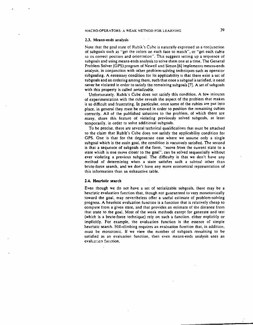
The usefulness of an evaluation function is directly related to its accuracy in estimating the distance to the goa\. In an effort to find a useful heuristic for Rubilc's Cube. several plausible candidates were tested experimentally to determine their accuracy. The surprising results were that none of the heuris­tics tested produced values that had any positive correlation with distance from the goal!

The basic idea of the experiment was to compute the average actual distance from the goal state for all the stales that produce a particular value of the given evaluation function. The 2 x 2 x 2 Rubik's Cube was used because the state space is small enough (3 million states) that it can be exhaustively searched. The first step of the experiment was to conduct a breadth-first search of the entire space. generating a table which lists the actual minimum distance of each state to the goal state. The maximum distance of any state from the goal is 11 moves. and the average distance over all states is 8.76 moves.

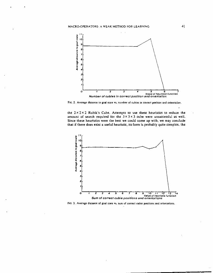
The next step was to identify plausible evaluation functions. which resulted in four fairly obvious ones. The first heuristic function is simply the number of cubies that are in their goal positions and orientations. Note that a cubie can be in its correct position but in an incorrect orientation. Considering position and orientation independently. the second function awards one point for a cubie in its goal position. one point for a cubie in its goal orientation. and two points for both. Reasoning that the position of a cubie relative to its neighbors in the goal state is more important than its absolute position. the next heuristic counts the number of pairs of adjacent cubies that are in the correct position and orientation relative to each other, without regard to their global position or orientation. Taking into account the distance of a cubie from' its goal position. the final evaluation function determines the minimum number of moves required to correctly position and orient each cubie independently. and sums these values over all the cubies.

The results of the experiments are presented as a set of graphs. one for each evaluation function (see Figs. 2 through 5). In each case. the x-axis of the graph corresponds to the different values produced by the heuristic function. The y-axis of the graph corresponds to the average distance from the goal state. Each data point gives the average distance from the goal state for the set of states which produce a particular value of the evaluation function.

The results show that in. general. the average distance from the goal for a set of states sharing a particular heuristic value is within 10% of 8.76. the average for the entire state space. This result holds across almost all values of all the evaluation functions. The only significant deviation from this norm is that the states whose evaluations are closest to that of the goal state are in fact further from the goal than the average state! However. none of the evaluation functions identify a set of states that are even a single move closer to the goal state. on the average.

This implies that none of the above heuristics are of any direct use in solving

MACRO·OPERA TORS: A WEAK METHOD FOR LEARNING

~If

; 10 ... ~ 9r-______________________________ ~ ; 8 u ~ 7 ;;; 'ii 6 ill Ol ~ 5 ill ,.

oct 4

3

2

02345 7 Value of heutisric funclion

Number of cubies in correct position and orientation

FIG. 2. Average distance to goal state vs. number of cubies in correct position and orientation.

41

the 2 x 2 x 2 Rubik's Cube. Attempts to use these heuristics· to reduce the amount of search required for the 3 x 3 x 3 cube were unsuccessful as well. Since these heuristics were the best we could come up with. we may conclude that if there does exist a useful heuristic, its fonn is probably quite complex, the

!! ~

'"

--0 Ol

~ ill u co ... ;;; 'ii ill Ol ~ ill ,.

oct

If

10

9

8

7

6

5

4

3

2

0 2 3 4 5 6 7 8 9 10 1 I 12 13 14 Value of I,eutistic function

Sum of correct cubie positions and orientations

FIG. 3. Average distance of goal state vs. sum of correct cubie positions and orientations.

42

CI ... OJ iO 0 CII

~ CI U 0:: ~ .. 'ii CI CII .. .. CI ,. ~

" 10

9

8

7

6

5

4

3

2

R.E. KORF

o 234557851 Va/uti of IIflu,istic function

Sum of adjacent cubie pairs correct relative to each other

FIG. 4. Average distance to goal state vs. sum of adjacent cubie pairs correct relative to each other.

limiting case being the heuristic of moving one step closer to the goal. Furthermore, none of the literature on the cube suggests any other evaluation functions. All this evidence suggests that heuristic evaluation functions are not in fact used to solve this problem.

3

2

o 2 3 4 5 5 7 If SI 10 I I 12 13 14 15 '5 17 18 'SI V"/uflof IIcu,istic function

Sum of distance of each cubie from correct position and orientation

FIG. S. Average distance to goal state vs. sum of distance of each cubie from correct position and orientation.

MACRO-OPERATORS: A WEAK METHOD FOR LEARNING 43

2.S. Conclusion

Since all the weak methods rely on some type of evaluation function, we conclude that Rubik's Cube is an example of a problem that cannot be solved by any of our current weak methods. It can. however, be solved effectively by people. Hence, either there exists an as yet undiscovered weak method, or a knowledge-based approach is required to solve the problem. The answer will prove to be both.

3. Previous Work

This section reviews previous work that has contributed to or is related to the development of the Macro Problem Solver. It includes the General Problem Solver, research on non·serializable subgoals in the context of the blocks world, the development of the idea of macro-operators, the ideas of Banerji for using macros to deal with non-serializable subgoals, an~ work on permutation groups.

3.1. The General Problem Solver

As described in Section 2, the General Problem Solver (GPS) of New~1I and Simon solves a problem by using an ordered set of sub goals and solving them

_ one at a time, such that the main goal can be reached without violating a previously solved subgoal. The structure of the Macro Problem Solver (MPS) borrows heavily from that of GPS, to the extent that the Macro Problem Solver is actually a generalization of GPS to include macro-operators in addition to primitive operators.

3.2. Non·serializable subgoals .

The problem of non-serializable subgoals was studied in the context of the blocks world by a number of researchers in the early 1970s. Sussman's HACKER

program [8] deals with problems of building stacks of blocks represented by sets of conjunctive subgoals of the form (On X Y). where X and Yare blocks. HACKER works by initially assuming that the subgoals can be achieved in­dependently and then explicitly invokes a set of 'debugging' mechanisms to deal with interactions between the subgoals. Subsequently. Warren [9]. Tate [10]. Waldinger [11). and Sacerdoti [12] arrived at related techniques for generating optimal plans for problems with non-serializable subgoals by poten­tially reordering all the subgoals and actions required to solve a conjunctive goal.

There are several limitations to this body of work in dealing with non­serializable subgoals. One is that most of these systems. with the exception of that of Waldinger, simply reorder the primitive actions necessary to achieve each of the subgoals independently, without the capability of adding new

R.E. KORF

actions to deal directly with subgoal interactions [12]. A second factor is that the subgoal interaction in the blocks world is not an inherent property of the domain but rather an artifact of the particular subgoals chosen to decompose a main goal. In particular, if we simply add a subgoal of the form (On X Table) where X is the bottom-most block of a stack, then all the block-stacking problems could be solved by GPS simply by first putting the bottom block on the table, then the next-higher block, and so on until the top block is placed on top of the stack. A final limitation is that these techniques only work on problems for which independence of subgoals is a good first approximation (8). For these reasons, it seems highly unlikely that these methods would be powerful enough to deal with the complexity of subgoal interactions manifested by a problem such as Rubik's Cube.

3.3. Macro-operators

The idea of composing a sequence of pTlmltlve operators and viewing the sequence as a single operator goes back to Saul Amarel's 1968 paper on representations for the Missionaries and Cannibals problem [13]. The first implementation of this idea is the use of MACROPS (14) in the STRIPS problem solver. The main contributions of that work with respect to macros are the powerful mechanisms for generalizing macros.

There are several features of the work on MACROPS that distinguish it from the research reported here~ The most important is that MACROPS are not used to overcome the problems of non-serializable subgoals but rather to improve the efficiency of the STRIPS problem solver in a domain, robot problem solving, for which there exists a good set of GPS differences. The fact that STRrPS with MACROPS performs rel,atively inefficiently in this simple domain suggests that the system is not powerful enough to handle more complex domains. A second limitation of STRIPS with MACROPS is that it does not generate a complete set of macros. MACROPS are generated by using the solutions to particular problems posed to the system, and serve to reduce but not eliminate the amount of search required on future problems. The questions of what problems to use in a training sequence, and how much search is still required to solve problems chosen from some population given a set of MACROPS, are difficult and still open. By contrast, the Macro Problem Solver works from a complete set of macros that eliminate search entirely.

The REf1..ECT system of Dawson and Siklossy [IS] has a preprocessing stage where macro-operators, called Bloops, are generated by comparing the post­conditions of each primitive operator with the preconditions of all possible successor operators, creating a two-operator macro whenever they match. Unfortunately, this approach is limited to very short macros or to operator sets where the preconditions severely constrain the possible operator sequences.

-.

MACRO-OPERATORS: A WEAK ~1ETHOD FOR LEARSING 45

3.4. Macros and non-serializable subgoals

The fact that macro-operators can be used to overcome the problem of non-serializable subgoals was first suggested by Banerji [(6). He points out that both Rubik's Cube and the Fifteen Puzzle cannot be solved by a straightfor­ward application of GPS. but that an extension of GPS to include macros would be able to solve these problems. Banerji suggests that at a given stage of a strategy. the macros that are useful are ones that leave all previously satisfied subgoals intact while satisfying an additional subgoal as well. Within the body of a macro, a previous subgoal may be violated. but by the end of the macro, the subgoal must be restored. Banerji's work was independent of and concur­rent with this research.

3.5. Permutation groups

Given that macros may be useful for solving problems with non-serializable subgoals, the issue of exactly what macros are necessary and how to use them in an efficient strategy must be addressed. A solution to this problem is suggested by the work of Sims [17] on computational problems of permutation groups. The goal of that research, and related work by others. is to be able to represent a permutation group compactly so that questions such as the order of the group and membership in the group can be answered efficiently.

Sims shows how a permutation group on n elements can be represented by an n x n matrix of permutations where the permutation in the jth row of the ith column maps the jth element to the ith position. and leaves the first i-I elements of the permutation invariant. Sims also implemented an algorithm to fill in the permutation table given a set of generators of the group. or primitive permutations. The technique relies on the observation' that if permutation A leaves the first i-I elements invariant and maps the jth element to the ith position, and permutation B has the same properties, then A composed with the inverse of B will leave the first i elements invariant.

Furst, Hopcroft, and Luks [18) later showed that the complexity of a similar algorithm for generating the permutations in this matrix is a polynomial of order n 6 where n is the number of elements permuted. Knuth2 reduced this upper bound to n

j log n, and Jerrum [19) further reduced it to n j for a slightly

different representation .. As we will see in Section 4, replacing the permutations in such a table with

corresponding sequences of primitive operators gives rise to an effective strategy for solving permutation problems. There are two limitations. however, to this work from the point of view of general problem solving. One is that it refers only to permutation groups and must be extended to apply to a broader

lpersonai communication from Donald Knuth to Eugene Luks. May 1981.

R.E. KORF.

class of problems. The second limitation of this work is that the technique used to fill in the permutation table results in extremely inefficient solutions. relative to human strategies. in terms of number of primitive moves. For example. in the case of the 3 x 3 x 3 Rubik's Cube, macros can be as long as 217 primitive moves.

3.6. Conclusion

In conclusion. we find that many of the main ideas in this anicle can be found in one form or another in the literature of problem solving. The basic structure of the problem solver comes from GPS. the study of non-serializable subgoals was pioneered in the blocks world, the use of macro-operators dates from Sl1tIPS, Banerji independently discovered the application of macros to non­serializable subgoals, and the structure of macro tables is borrowed from work on permutation groups. The novel contributions of this work ,are the com­bination of these ideas into a general problem-solving and learning method, and a precise theory of the applicability and performance of the technique.

4. The Macro Problem Solver

This section describes the operation of the Macro Problem Solver and gives several examples of its use. BrieHy. the problem solver achieves an ordered set of subgoals one at a time by applying macros that solve the next subgoal while leaving previously solved sub goals intact, even though they may be temporarily violated during the application of the macro. We describe a problem represen­tation, the structure of the table of macros, and the problem-solving algorithm.

·The issue of how the macros are learned will' be deferred to the following section. The collection of examples includes the Eight and Fifteen Puzzles, Rubik's Cube, the Think-a-Dot problem, and the Towers-of-Hanoi problem. For simplicity of exposition, the Eight Puzzle will be used as the primary example.

The Eight Puzzle (see Fig. 6) has been studied extensively in the anificiaI intelligence literature [20-22] and provides one of the simplest examples of the operation of the Macro Problem Solver. It consists of a three-by-three frame which contains eight numbered square tiles. One of the squares of the frame is

ffi81 Z l

II 4

7 II 5

FIG. 6. Eighl Puule goat Siale.

MACRO-OPERATORS: A WEAK ~fETHOD FOR LEAR~ING 47

empty; this is referred to as the blank tile or blank. Any of the tiles horizon­tally or vertically adjacent to the blank can be moved into the blank position. The problem is to take an arbitrary initial configuration of the tiles and transform it into a goal state. such as that shown in Fig. 6, by sliding the tiles one at a time.

4.1. The stat~vector representation

We begin with an abstract representation of our example problems. A state of a problem is specified by the values of a vector of state variables. Banerji [16] argues that this representation is natural and very general. For example. the state variables for the Eight Puzzle are the nine different tiles of the puzzle. including the blank, and the values are the positions occupied by each tile in a particular state. For Rubik's Cube. the variables are the different cubies, and the values encode both the position and the orientation of the cubies. In the case of the Towers of Hanoi, the variables are the disks. and the values are the pegs that the disks are on. For each problem, a single goal state is specified by assigning particular values to the state variables. called their goal values.

Note that a dual representation exists for these problems. and may in fact seem more intuitive to the reader. For example. in the Eight Pu~le the variables could correspond to the positions and the values could represent the tiles which occupy the positions. The two representations are isomorphic. but the macro problem-solving technique is sensitive 'to the representation of the problem and in general will not work in the dual representation, as will be discussed in Section 6. Thus. we will use the original representation described above.

4.2. The macro table

Table 1 shows a macro table for the Eight Puzzle. corresponding to the goal state in Fig. 6. The columns correspond to the tiles and the rows correspond to the tile positions. The labels of the positions coincide with the numbers of the tiles that occupy them in the goal state. The elements of the table are macros. which are sequences of primitive moves. A primitive move is represented by the first letter of Right. Left. Up. or Down, and is the direction that a tile is moved. This notation is unambiguous since only one tile. other than the blank. can be moved in each direction from any given stale.

The subgoals used to solve the problem are the obvious ones of placing the tiles in their correct positions one at a time. or in other words. mapping the state variables to their goal values sequentially. The first thing that must be decided is the solution order, or the order in which the tiles are to be positioned. The constraints on solution orders will be discussed in detail in Section 6. Briefly. the constraint is that the applicability and the effect of any operator on any state variable must be a function only of that state variable

tJO

TABLE l. Macro lable for Ihe Eighl Puzzle. The 10lal nu~ber of non-idenlilY macros is 35. The average case solulion lenglh is 39.78 moves

0

I 2

~J o· 0:;' .. °

~s 6 7 II

0

UL U UR R DR D DL L

RDLU DLURRDLU LDRURDLU ULDRURDLDRUL URDLDRUL RULDDRUL DRUL

2

DLUR LDRV LURDLDRU ULDDRU DRUULDRDLU RULLDDRU

Tiles

J

RDLLURDRUL WRULURDDLUR URDDLULDRRUL RULDRDLULDRRUL RDLULDRRUL

..

LURD ULDR URDLULDR RULLDR

s

RDLLUURDLDRRUL ULDRURDLLURD ULDRRULDLURI>

6

lJRDL RULD

MACRO-OPERATORS: A WEAK METHOD FOR LEARNING .t9

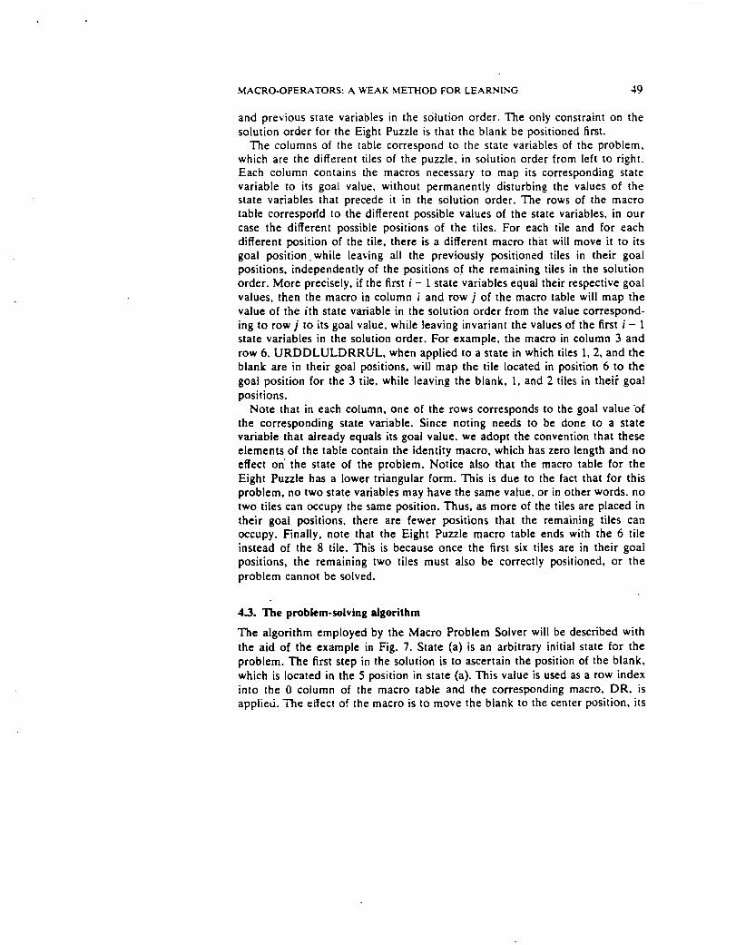
and previous state variables in the solution order. The only constraint on the solution order for the Eight Puzzle is that the blank be positioned first.

The columns of the table correspond to the state variables of the problem. which are the different tiles of the puzzle. in solution order from left to right. Each column contains the macros necessary to map its corresponding state variable to its goal value. without permanently disturbing the values of the state variables that precede it in the solution order. The rows of the macro table correspond to the different possible values of the state variables. in our case the different possible positions of the tiles. For each tile and for each different position of the tile. there is a different macro that will move it to its goal position. while leaving all the previously positioned tiles in their goal positions. independently of the positions of the remaining tiles in the solution order. More precisely. if the first i-I state variables equal their respective goal values. then the macro in column i and row j of the macro table will map the value of the ith state variable in the solution order from the value correspond­ing to row j to its goal value. while leaving invariant the values of the first i-I state variables in the solution order. For example. the macro in column 3 and row 6. URDDLULDRRUL. when applied to a state in which tiles 1.2, and the blank are in their goal positions. will map the tile located in position 6 to the goal position for the 3 tile. while leaving the blank, 1, and 2 tiles in their goal positions.

Note that in each column. one of the rows corresponds to the goal value 'of the corresponding state variable. Since noting needs to be done to a state variable that already equals its goal value. we adopt the convention that these elements of the table contain the identity macro. which has zero length and no effect on' the state of the problem. Notice also that the macro table for the Eight Puzzle has a lower triangular form. This is due to the fact that for this problem. no two state variables may have the same value. or in other words, no two tiles can occupy the same position. Thus. as more of the tiles are placed in their goal positions. there are fewer positions that the remaining tiles can occupy. Finally. note that the Eight Puzzle macro table ends with the 6 tile instead of the 8 tile. This is because once the first six tiles are in their goal positions. the remaining two tiles must also be correctly positioned. or the problem cannot be solved.

4.3. The problem-solving algorithm

The algorithm employed by the Macro Problem Solver will be described with the aid of the example in Fig. 7. State (a) is an arbitrary initial state for the problem. The first step in the solution is to ascertain the position of the blank. which is located in the 5 position in state (a). This value is used as a row index into the 0 column of the macro table and the corresponding macro. DR. is applieu. The effect of the macro is to move the blank to the center position. its

50

§1§

•

co I 0 rOillf S

OR

co I • row"

~ col 1

~ row Z ROLU

~ eol5 ~ row 7 A

1 UlORUROllURO

co I Z row 7

·OnUUlOROlU

co I 6 row 7 UROl

~

FKi. 7. Example of soI~tion of tbe Eijht Puzzle by the MaI;ro Problem Solver.

R.E. KORF

co I 3 row 3

goal location. Next, the location of the 1 tile in state (b) is ascertained, position 2 in our example, this value is used as a row index into column 1 of the macro table, and the corresponding macro is applied. The effect of this macro is to move the 1 tile to its goal position. while leaving the blank at its goal position. Note that during the application of the second macro the blank is moved. but by the end of the macro application. the blank is restored to the center position. Similarly. the position of the 2 tile in state (c) is used to select a macro from column 2 that will map the 2 tile to its goal position while leaving the blank and 1 tiles in their goal positions. Note that in state (d), the 3 tile happens to be in its goal position already and hence the identity macro is applied. as is the case for tile ~ in state (e). In general. for i from 1 to n, if i is the value of variable i in the solution order. apply the macro in column i and row i, and then repeat the process for the remaining variables. Note that the value of variable i above refers to its value at the jth stage of the solution process, and not to its value in the initial state.

This solution algorithm will map any solvable initial state to the given goal state. The algorithm is deterministic, i.e. it involves no search. and hence is very efficient. running in time proportional to the number of primitive opera­tors that are applied in the solution. It derives its power from the knowledge about the problem that is contained in the macros.

Unfortunately. the actual macro table is dependent on the particular goal state that is chosen. The algorithm can be simply extended. however, to allow mapping any initial state to any goal state. The idea is to first find a solution from the initial state to the goal state for which the macro table was generated. then find a solution from the desired goal state to the goal state of the macro table. and finally compose the first solution with the inverse of the second solution. The inverse of a sequence of primitive operators is obtained by replacing each operator with its inverse and reversing the order of the opera­tors. Hence. if each of our primitive operators has a primitive inverse, ·we can

MACRO-OPERATORS: A WEAK METHOD FOR LEARNING 51

use the Macro Problem Solver to m"ap any initial state to any goal state with a penalty of approximately doubling the solution length.

4.4. Additional examples

This section presents several additional example problems for which the Macro Problem Solver is effective. They include the Fifteen Puzzle, Rubik's Cube. the Think-a-Dot problem, and the Towers-of-Hanoi problem.

4.4.1. Fifteen Puzzle

Since the size of the state space for the Eight Puzzle is fairly small (181440 states). a macro table for the Fifteen Puzzle was also generated to show the power of the technique in larger domains (about 1012 states). Unfortunately, space limitations prohibit its inclusion here and the interested reader is referred to [4]. The table contains 119 macros, the longest of which is 24 moves long. and produces an average case solution length of 139.40 primitive moves. While this example provides no new insights into the operation of the Macro Problem Solver. it does present additional problems to the learning program as we will see in the following section.

4.4.2. Rubik's Cube

For reasons already mentioned, Rubik's Cube was the primary vehicle for the development of the Macro Problem Solver. The state variables for this problem are the individual cubies, and the values encode both the positions and the orientations of the cubies. The subgoals are to position and orient the cubies correctly one at a time. . .

Again, space constraints prevent including the complete macro tables here. The 2 x 2 x 2 table contains 75 macros, ranging in length from 1 to 11 moves, and produces an average case solution length of 27 primitive moves. The 3 x 3 x 3 macro table is composed of 238 macros up to 14 moves long and generates an average case solution length of 86.38 primitive moves.

4.4.3. Think -a-Dot

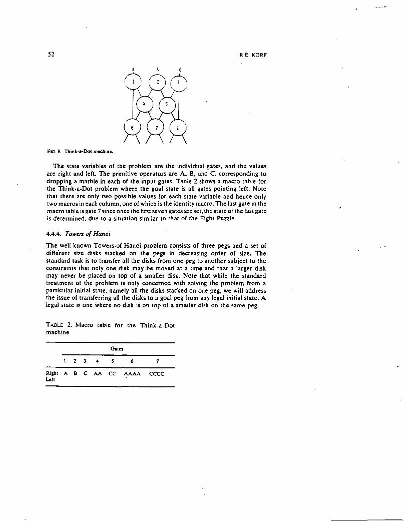
The Think-a-Dot machine was a commercially available toy which involves dropping marbles through gated channels and observing the effects on the gates. Fig. 8 is a schematic diagram of the device. There are three input channels at the top, labelled A, B, and C, into which marbles can be dropped. When a marble is dropped in. it falls through a set of channels governed by eight numbered gates. Each gate has two states. left and right. When a marble encounters a gate, it goes left or right depending on the current state of the gate and then flips the gate to the opposite state. A state of the machine is specified by giving the states of each of the gates. The problem is to get from an arbitrary initial state to some goal state, such as all gates pointing left.

52 R.E. KORF

FlO. 8. Think-a-Dot madline.

The state variables of the problem are the individual gates. and the values are right and left. The primitive operators are A. B, and C. corresponding to dropping a marble in each of the input gates. Table 2 shows a macro table for the Think-a-Dot problem where the goal state is all gates pointing left. Note that there are only two possible values for each state variable and hence only two macros in each column. one of which is the identity macro. The last gate in the macro table is gate 7 since once the first seven gates are set. the state of the last gate is determined. due to a situation similar to that of the Eight Puzzle.

4.4.4. Towers of Hanoi

The well-known Towers-of-Hanoi problem consists of three pegs. and a set of diffe'rent size disks stacked on the pegs in 'decreasing order of size. The standard task is to transfer all the disks from one peg to another subject to the constraints that only one disk may be moved at a time and that a larger disk may never be placed on top of a smaller disk. Note that while the standard treatment of the problem is only concerned with solving the problem from a particular initial state. namely all the disks stacked on one peg, we will address the issue of transferring all the disks to a goal peg from any legal initial state. A legal state is one where no disk is on top of a smaller disk on the same peg.

TABLE 2. Macro table for the Think-a-Dot machine

2 J .. 6 7

Right ABe AA ee AAAA ecce Left

MACRO·OPERATORS: A WEAK ~fETHOD FOR LEARNING

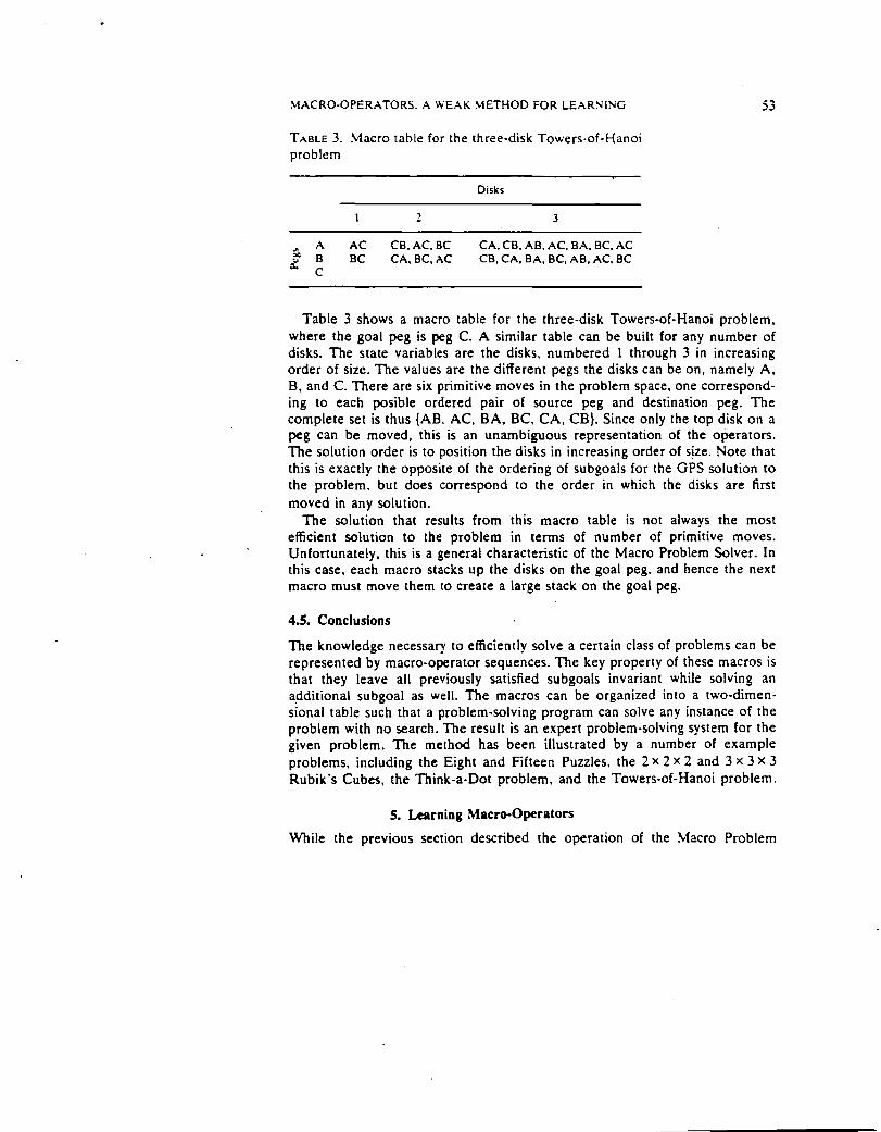
TABLE 3. Macro table for the three-disk Towers-of-Hanoi problem

.., A E B

C

AC BC

2

CB.AC.BC CA. BC.AC

Disks

3

CA. CB. AB. AC. BA. BC. AC CB. CA. BA. BC. AB. AC. BC

53

Table 3 shows a macro table for the three-disk Towers-of-Hanoi problem. where the goal peg is peg C. A similar table can be built for any number of disks. The state variables are the disks. numbered 1 through 3 in increasing order of size. The values are the different pegs the disks can be on. namely A. B. and C. There are six primitive moves in the problem space. one correspond­ing to each posible ordered pair of source peg and destination peg. The complete set is thus {AB. AC. BA. BC. CA. CB}. Since only the top disk on a peg can be moved. this is an unambiguous representation of the oPerators. The solution order is to position the disks in increasing order of sjze. Note that this is exactly the opposite of the ordering of subgoals for the GPS solution to the problem. but does correspond to the order in which the disks are first moved in any solution.

The solution that results from this macro table is not always the most efficient solution to the problem in terms of number of primitive moves. Unfortunately. this is a general characteristic of the Macro Problem Solver. In this case. each macro stacks up the disks on the goal peg. and hence the next macro must move them to create a large stack on the goal peg.

4.5. Conclusions

The knowledge necessary to efficiently solve a certain class of problems can be represented by macro-operator sequences. The key property of these macros is that they leave all previously satisfied sub goals invariant while solving an additional subgoal as well. The macros can be organized into a two-dimen­sional table such that a problem-solving program can solve any instance of the problem with no search. The result is an expert problem-solving system for the given problem. The method has been illustrated by a number of example problems. including the Eight and Fifteen Puzzles. the 2 x 2 x 2 and 3 x 3 x 3 Rubik's Cubes. the Think-a-Dot problem. and the Towers-of-Hanoi problem.

5. Learning Macro-Operators

While the previous section described the operation of the Macro Problem

54 R.E. KORF

Solver once it has a complete macro table. this section is concerned with the problem of how the macros are acquired. This is the learning component of the paradigm. The basic technique that will be used is to search the space of macro-operators. Each macro generated is inserted into the macro table in its correct slot. unless a shorter macro already occupies that slot. We first address the problem of where to place a given macro in the macro table. We then consider three different methods for generating macros. One is a simple brute·force search through the space of primitive operator sequences. the second is a variation of bi-directional search. and the last is the macro composition technique of Sims [17].

5.1. Asslpina macros to the macro table

In general. the macros that make up the macro table all have the property that they leave an initial sequence of the state variables invariant if they equal their goal values. and map the next state variable to its goal value. independent of the values of the remaining variables in the solution order. In addition. the table should ideally be filled with the shortest macros that accomplish each sub goal. This section is concerned with the problem of determining the correct location in the table of a given macro.

5.1.l. Seucting the column

In order to determine the column in the macro table in which" an arbitrary macro belongs. we introduce the notion of the invariance of a macro. Given a particular goal state. a solution order. and a macro-operator. we define the invariance of the macro as follows: The macro is applied to the goal state of the problem and the resulting state is compared with the goal state. The itIVariance of the macro is the length of the longest initial sequence. according to the solution order. of state variables that equal their corresponding goal values. The sequence starts with the first state variable in the solution order and continues until a mismatch is found. In other words. if the first state variable of the resulting state does not equal its goal value. the invariance of the macro is zero; if the first variable in the solution order equals its goal value but the second does not. the invariance of the macro is one; and in general if the first i state variables in the solution order equal their goal values but the (i + l)st does not. then the invariance of the macro is i. For example. if the goal state of the Eight Puzzle is represented by the vector [B. 1, 2. 3. 4, 5. 6, 7. 8]. the solution order is (B. 1. 2., 3. 4, 5, 6. 7, 8). and the state resulting from the application of some particular macro to the goal state is [B, 1. 2., 3. 6. 5. 7. 4, 8], then the invariance of the macro is four. because the first four tiles (including the blank) in the solution order are in their goal positions and the fifth is not.

The invariance of a macro gives the longest initial sequence of state variables in the solution order that are left invariant by the application of the macro to

MACRO·OPERA TORS: A WEAK METHOD FOR LEARNING 55

the goal state. Hence, the invariance of a macro determines its column in the macro table.

5.1.2. Selecting (he row

In addition to the column, we must also determine the proper row for a macro in order to include it in the macro table. A macro in column i and row j of the macro table, when applied to a state in which the first i variables in the solution order equal their goal values and in which the (i + l)st variable equals the value corresponding to row j, results in a state in which the first i + 1 variables equal their goal values. Hence, the row in the table of a macro with invariance i is the row that corresponds to the value of the (i + l)st state variable that the macro maps to its goal value.

If a macro has invariance i, then its inverse will also have invariance i, where the inverse is obtained by reversing the order of the operators and replacing each with its inverse operator. The reason is that the original macro maps the first i variables from their goal values back to their goal values and hence the inverse must do the same. Second, if the (i + l)st state variable has the value corresponding to row j after the application of the inverse macro to the goal state, then the correct row of the original macro in the macro table is' j. The reason is that the inverse macro maps the value of the (i + l)st variable from its goal value to that corresponding to j, and hence the original macro would map the value corresponding to j back to the goal value. Thus, given a macro with invariance i, we place it in the table at column i, and at the row which corresponds to the value of the (i + l)st variable in the solution order when the in-.:erse macro is applied to the goal state.

S.2. Brute-force search

Given the above techniques for placing a macro in its correct place in the macro table, what is still required for the learning program is a method of generating macros. Since we are interested in the shortest possible macros for each slot in the table, we first adopt a brute-force, depth-first, iterative­deepening search from the goal state. Depth-first, iterative·deepening is a search algorithm which first expands the first level of the search tree, then performs a depth-first search to level two, followed by a depth-first search to level three, etc. It uses far less memory than breadth-first search, yet always finds a shortest path to the goal. Thus, the first macro placed in each empty slot in the table is guaranteed to be a minimal length macro for that slot.

It is important to realize that a single search from the goal state will find all the macros in the table, and that a separate search for each column or even each entry is not required. We are not searching for particular states but rather for particular operator sequences. For problems like Rubik's Cube that have no preconditions on the operators, a single search will encounter all possible

56 R.E. KORF

operator sequences up to the length of the search depth, and ·hence will find all macros up to that length. For problems with operator preconditions, such as the Towers·of-Hanoi problem. recall that we are Dnly interested in macros that map some initial subsequence of the state variables in the solution order t6 their goal values. Hence, by searching from the complete goal state and using the inverses of the operator sequences generated, we will find all the macros in a single search.

One problem with this learning algorithm is knowing when to terminate it. We cannot simply run it until all the slots in the macro table are filled because some slots may remain permanently empty. For example, the last two columns of the Eight Puzzle macro table can never be filled, due to the property of the puzzle that the positions of the last two tiles are determined once the positions of the remaining tiles are known. Both Rubik's Cube and the Think-a-Dot problems have similar properties. In general, discovering these properties is very difficult. Hence, we have a situation of not knowing when we know enough to solve every instance of the problem.

There are several solutions to this difficulty. One is simply to run the learning program until its computational resources, in most cases memory, are exhaus· ted. Another is the heuristic of terminating the search if one or two additional plies fail to produce any new macros. The best solution involves interleaving the learning program with the problem-solving program as co-routines and only running the learning program when a new macro is needed to solve some particular problem instance.3

Brute·force depth-first iterative-deepening is sufficient to solve the Eight Puzzle, the Towers-of·Hanoi, and the Think·a-Dot problems. For problems as large as the Fifteen Puzzle and the Rubik's Cubes, however, a more sophisti­cated technique is required.

5.3. Partial-match, bi-dlrectional search

If we assume that each primitive operator has an inverse primitive operator, thus ruling out the Think·a-Dot example, then we can find macros considerably more efficiently than by depth-first iterative-deepening. Consider a macro that leaves i state variables invariant. When applied to the goal state, the values of these state variables are mapped from their goal values, through a succession of intermediate values, and finally back to their goal values again. Now split in half the sequence of primitive operators that make up the macro. The first half maps the i state variables from their goal values to a sequence of values (VI' V2, •.. , vj ), and the second half maps these values back to their goal values. Thus, the inverse of the second half of the macro will map the goal values of these variables to this same set of values (VI' v2' ... , vJ This suggests that, given

>-tbis was suggested by Jon Bentley.

~fACRO-OPERA TORS: A WEAK METHOD FOR LEARNING 57

two different macros that map the same initial subsequence of i state variables. according to the solution order, from their goal values to an identical vector of intermediate values, composing one of the macros with the inverse of the other will yield a macro with invariance i. Thus. macros can be found by storing the intermediate values of the state variables for each macro when applied to the goal state and comparing them with the corresponding values for each new macro generated. looking for matches among initial subsequences of variables according to the solution order.

Note that once a match is found, two macros can be generated. depending on which of the two matching submacros is inverted. The two macros are inverses of each other. Hence. each of these macros must have the same invariance. but in general the rows of the macro table to which they belong may be different. Furthermore, by using the inverse method for determining the row of a macro. the correct row for each of the macros can easily be determined from the other. Note that this is not a heuristic method but is in fact guaranteed to find all minimal-length macros, since every macro can be split into two parts as described.

This scheme is closely related to bi-directional search. first analyzed by Pohl [23]. They have in common searching for a path from both ends simul­taneously. looking for a match between states generated from opposite direc­tions, and then composing the path from one direction with the inverse of the path from the other direction. There are, however. three important differences between this technique and bi-directional search. One is that in this case the initial and goal states are the same state. namely the goal state, and hence only one search is necessary instead of two. The second difference is that, since we are looking for macros that leave only some' initial subsequence of the state variables invariant. we only require a partial match of the state variables rather than a total match. Finally, in order to save space and find the shortest macros, the bi-directional search is combined with depth-first iterative-deepening.

The computational advantage of this scheme is tremendous. In order to find a macro of length d. instead of searching to depth d, we need only search to depth r d/2l. Since the computation time for a complete depth-first search is proportional to bd

, where b is the branching factor and d is the depth of the search, this reduces the computation time from bd to btln

• essentially halving the exponent.

However, if each new state must be individually compared to each existing state, a bi-directional search requires as much time as a uni-directional search. with the comparisons taking up most of the time. Thus, the performance claimed above can only be achieved if a new state can be compared to all the existing states in constant time. Fortunately, hashing the states based on the values of the state variables achieves this performance.

An alternative scheme for comparing the generated states efficiently uses a search tree instead of a ha£h table. As each state is generated, it is stored in a

58 R.E. KORF

tree where each level of the tree corresponds to a different state variable and different nodes at the same level correspond to ~ifferent possible values for that state variable. The ordering of levels of the tree from top to bottom corresponds to the solution order of the state variables from first to last. Thus, each node of the tree corresponds to an assignment of values to an initial subsequence of state varia~les in the solution order.

A state is inserted in the tree by filtering it down from the root node to the last existing node which corresponds to a previously generated state. A new node is created at the next level of the tree and the macro which generated the new state is stored at the new node. Since the states are generated using iterative deepening, this ensures that stored with each existing node is a shortest macro which maps the goal state to the initial subsequence of values corresponding to that node. When a new state reaches the last previously existing node it matches in the tree, a macro is created as before.

The expected number of probes to compare a new state to the existing states for the hashing scheme is constant, assuming the hash table re.mains partly empty [24]. For the search tree, the expected number of comparisons is linear in the number of state varjables. The partial-match, iterative-<ieepening, bi­directional search algorithm is sufficient to find all the macros for the Fifteen Puzzle and the 2 x 2 x 2 Rubik's Cube. The limitation of this algorithm, as for any bi-directional search. is the amount of memory available fOJ storing states.

5.4. Macro composition

Finding all the macros up to length nine for the 3 x 3 x 3 Rubik's Cube macrQ table requires storing about 50 000 states. This stillle'aves seven empty slots, out of 238, in the table. These remaining slots can be filled using the macro­composition technique employed by Sims [17].

If we compose two macros with invariance i, the result will also be a macro with invariance at least i, but in general a different macro. If, in addition, when the macros are applied to the goal state the two (i + l)st state variables take on the same values, but not necessarily the goal values, then if we compose either macro with the inverse of the other macro, the result will be a maCTO with invariance at least i + 1. This is actually just a special case of the more general technique described in the previous section, specialued in the sense that not only are the first j variables constrained to match, but they must equal the goal values as well.

The advantage of this technique is that it allows us to find macros with high invariance with very little computation, by using macros with high invariance that have already been found. The disadvantage of the technique is that a macro found by this method will not in general be the shortest macro for the corresponding slot in the macro table. There is some psychological plausibility to this method for finding macros in that many human cube solvers, particularly

MACRO·OPERATORS: A WEAK METHOD FOR LEARNING 59

novices, use compositions of shorter macros to complete the final stages in their solution strategies. ' .

The macro·composition technique is effective in finding the remaining seven macros for Rubik's Cube that are beyond the range of the bi·directional search. Most of these macros are fourteen moves long whereas macros twelve moves long are known to exist for these slots in the table. The complete learning program for the 3 x 3 x 3 Rubik's Cube runs for less than 15 minutes of CPU time on a V AX/ll·780 and uses about 200K words of memorv.

Note that macro composition could be used to find all the m~cros for Rubik's Cube, starting with only the primitive operators of the problem. However. as pointed out in Section 3.5, the resulting strategy would be extremely inefficient in terms of number of primitive moves. The combination of bi·directional search and macro composition amounts to a tradeoff between learning time and space vs. solution efficiency.

5.5. Conclusions

We have presented a number of techniques for learning macros effectively. These include brute-force iterative-deepening search. a variation of bi-direc­tional search that is only single-ended and requires only a partial ma'tch of the states, and the macro-composition technique of Sims. The performance of the learning program is limited by the amount of available memory. The most important results of this section are that all the macros in the table can be found in a single search from the goal state and that filling the macro table is feasible for problems of substantial size (e.g. the 3 x 3 x 3 Rubik's Cube).

6. The Theory of Macro Problem Solving

We have seen that macro problem solving works for a set of example problems, and have demonstrated the learning of macro-operators. We now tum our attention to the question of why these techniques work. The reason for addressing this issue is twofold: to understand the problem structure it is based on, and to characterize the range of problems for which it is effective. The main contribution of this section is to identify a property of problem spaces called operator decomposability. Roughly, operator decomposability exists in a prob­lem space to the extent that the effect of an operator on a state can be decomposed into its effect on each individual component of the state, in­dependent of the other components of the state. It will be shown that operator decomposability is a sufficient condition for the application of macro problem solving.

6.1. General definitions

We begin the formal theory with precise definitions of what is meant by a

60 R.E. KORF

problem. a problem instance. and a macro. In general. capital fetters will be used to denote sets. bold face will be used for vectors and vector functions .. and light face will be used for scalars and scalar functions.

Definition 6.1. We define a problem P to be a triple (5. O. g) where: 5 is a set of states and each state s E 5 is a vector of state variables

(SI' s: • ...• s~). where the Sj are chosen from a set of values V = {vI' vz • ...• Vh};

o is set of operators where each operator 0 E 0 is a total function from 5 to 5. In the event that there are preconditions on the operators. then V s E Sand o E 0 S.t. s does not satisfy the preconditions of operator o. we adopt the convention that o(s) =- s.

g E S is a particular state called the goal state, represented by the vector (gl' g20' .•• g~). where each gj is called the goal value of variable i.

In addition. let Sj be the set of all states in which the first i-I state variables equal their goal values or

s E 5 j iff s E Sand Vx. 1 05i x 05i j - 1, s. = g%.

Similarly. let 5q be the subset of Sj in which the ith state variable has value j, or

s E Sij iff s E 5 j and Sj = j.

Definition 6.2. A problem instance p is a pair (P. Sie;.) of a problem P and a particular initial state siM' .

Definition 6.3. A macro is a finite sequence of operators (01' °1, ••• , 0t) chosen from O. We write III(S) = t to denote the application of macro III to state s, where t = 0t ( ••. (01(0 1(1») .•• ). If Ie is zero, III is the identity macro I such that "1/ s E S, I(s)'" s.

Finally. we restrict the set of states of a problem to those that are solvable in the sense that:

V S E S, 3 a macro III S.t. III (s) = g .

6.2. Macro table definition

When we examine the macro table for the Eight Puzzle (Table 1). we notice that the first column contains nine entries. including the identity macro. There is one macro for each possible position that the blank could occupy in the initial state. or one macro for each possible value of the first state variable. Thus. the choice of what macro to apply first depends only on the value of the first state variable. Another way of looking at this is that for a given value of the first state variable. the same macro will map it to its target value regardless

MACRO·OPERATORS: A WEAK METHOD FOR LEARNING 61

of the values of the remaining state variables. In general, this property would not hold for an arbitrary problem. In fact, in the worst case. one would need a different macro in the first column for each different initial state of the problem. [n the second column as well, we only need one macro for each possible value of the second state variable (the positions of the 1 tile). Again, this is due to the fact that its application is independent of the values of all succeeding variables in the solution order. Similarly. for the remaining columns of the table. the macros depend only on the previous state variables in the solution order and are independent of the succeeding variables. More formally:

Definition 6.4. A macro table M is a set of macros, each denoted by mil for 1 :!SO j :!SO nand j E V. where mil is defined as follows:

If SII = 0. then mij is undefined. Otherwise, if Sli yi 0, then

Note that if j = gi' then mq = 1. the identity macro.

The property that allows macro tables to exist is called operator decom­posabi�ity. For pedagogical reasons. we first present a special case of operator decomposability called total decomposability.

6.3. Total decomposabiUty

Given that each state is a vector of the form (s\. S2' •••• s.), we define total decomposability as follo~s:

Definition 6.5. A vector ftinction 1 is totally decomposable if there exists a set of scalar functions Ii for l:!SO j :!SO n such that

v $ E S./($) = I(s\. S2' •••• s~) = UI(S\). UsJ . ... I. (s.» .

This property is illustrated by the operators of Rubik's Cube. Recall that the state variables are the individual cubies and the values encode their positions and orientations. Each operator will affect some subset of the cubies or state variables. and leave the remaining state variables unchanged. However, the resulting position and orientation of each cubie as a result of any operator is solely a function of that cubie's position and orientation before the operator was applied. and independent of the positions and orientations of the other cubies. Incidentally. for Rubik's Cube all the h are identical.

It can be shown that if all the operators of a problem are totally decompos­able, then there exists a macro table for the problem. However. total decom­posability is merely a special case of a more general property. called serial decomposability, for which we will prove the general result.

62 R.E. KORF

6.4. Serial decomposability

The small number of macros in the macro table is due to the fact that the effect of a macro on a state variable is independent of the succeeding variables in the solution order. However. the effect of a macro on a state variable need not be independent of the preceding variables in the solution order. since these values are known when the macro is applied. This suggests that a weaker and more general form of operator decomposability would still admit a macro table. This is the case with the Eight Puzzle. the Think-a-Dot problem, and the Towers-of· Hanoi problem.

Recall that in the Eight Puzzle. the state variables correspond to the different tiles, including the blank. Each of the four operators (Up, Down. Left. and Right) affect exactly two state variables. the tile they move and the blank. While the effects on each of these two tiles are totally decomposable. the ~conditions of the operators are not. Note that while there are no pre­conditions on any operators for Rubik's Cube, i.e. all operators are always applicable. the Eight Puzzle operators must satisfy the precondition that the blank be adjacent to the tile to be moved and in the direction it is to be moved. Thus. whether or not an operator is applicable to a particular tile variable depends on whether the blank variable has the correct value. In order for an operator to be totally decomposable. the decomposition must hold for both the preconditions and the postconditions of the operator.

The obvious solution to this problem is to pick the blank tile to be first in the solution order. Then. in all succeeding stages the position of the blank will be known and hence the dependence on this variable will not affect the macro table. The net result of this we~ker form of operator dec9mposability is that it places a constraint on the possible solution orders. The constraint is that the state variables must be ordered such that the preconditions anc:l the effects of each operator on each state variable depend only on that variable and preceding state variables in the solution order. If such an ordering exists. we say that the operators exhibit urial decomposability. In the case of the Eight Puzzle. the only constraint is that the blank must occur first in the solution order.

The following is a formal treatment of serial decomposability. It shows that serial decomposability is a sufficient condition for the existence of a macro table.

Definition 6.6. A solution order is a permutation 11 of the state variables of a state vector. Since we will never refer to more than one solution order at a time, without loss of generality we will continue to refer to a state as a vector of state variables (s\. S2' •••• s.) with the assumption that the order of the subscripts corresponds to the order of the state variables in the solution order under consideration.

MACRO-OPERATORS: A WEAK METHOD FOR LEARNING 63

Definition 6.7. A function I is serially decomposable with respect to a particular solution order 1T if there exists a set of vector functions I. for 1 ~ i ... n, where each Ii is a function from V' to V. and V' is the set of i-ary vectors with components chosen from V, which satisfy the following condition:

Lemma 6.8. A macro m is serially decomposable with respect to a solution order 1T if each of the operators in it are serially decomposable with respect to 1T.

Proof. In order to prove this result. if sufficies to show that the composition of two serially decomposable functions with respect to a solution order 11' is also serially decomposable with respect to 1T.

Assume that g and h are serially decomposable functions with respect to a solution order 1T, and that I is the composition of g and h. Then

m(5) = g(h(s» = g(h(s\. S2" ..• s~»

= g(h\(s\). h2(s\. s:J . .... h~(s\. S2' •••• s~»

= (g\(h\(s\».g2(h\(s\). h2(s\. s:J) •... , g~(h\(s\). "2(SI' s:J •...•

"~(Sl' S2' ••.• s.)))

where Ii and hi are the i·ary vector functions '!Vhich correspond to g and h. respectively. Hence I is serially decomposable with respect to 1T. 0

Definition 6.9. A problem P is serially decomposable if there exists a solution order fr such that V 0 E D. 0 is serially decomposabl~ with respect to fr.

The following theorem is the main theoretical result of this research.

Theorem 6.10. II a problem is serially decomposable, then there exists a macro table for the problem.

Proof. To prove the existence of a macro table M. it must be shown that for each i and j. IfI/I is either undefined or exists according to Definition 6.4. Hence, Vi.. j for 1 .s;; i .s;; nand j E V. either:

Case 1. SII = 0 in which case IfI, is undefined; or Case 2. S/j yIt 0 in which case 3.1 E Sii' Since all states are solvable by

definition, there exists a macro m S.t. m(.s) = I. Recall that

V .I E S" s, = g, for 0 :$0 y ~ i-I. and Sl = j.

Since s E S//, m (.I) = I. g = (g .. g2' ...• g.). and m is serially decomposable. then

64 R.E. KORF

and

where III, and lIIi are the y-ary and i-ary functions. respectively. corresponding to III. This is true independent of the values of S HI through S~. Therefore.

v s E Sv- III,(SI' 520 •••• 5,) = g, for 0 .... y :Iii i.

Thus,

Hence. III satisfies the definition of III il • 0

Note that total decomposability is merely a special case of serial decom­posability. Rubik's Cube is totally decomposable and hence any solution order admits a macro table.

While the Eight Puzzle is the simplest example of a serially decomposable problem. the Think-a-Dot machine exhibits a much richer form of serial decomposability that results in a complex constraint on the solution order. Roughly. the effect of an operator on a' particular gate can depend on the values of the gates above it. More exactly. the effect of an operator on a particular gate depends only on the values of all of its 'ancestors', or those gates from which there' exists a directed path to the given gate. Thus, the constraint on the solution order is that the ancestors of any gate must occur prior to that gate in the order. The serial decomposability structure of this problem is directly exhibited by the directed-graph structure of the machine. Note that the serial decomposability of this problem is based on the effects of the operators and not on their preconditions. since there are no preconditions on the Think-a-Dot operators.

An extreme case of serial decomposability occurs in the Towers-of-Hanoi problem. Recall that the variables correspond to the disks and the values correspond to the pegs. There are six operators. one for each possible ordered pair of source peg and destination peg. Since no smaller disk may be on the source or destination peg of the disk to be moved. the applicability of each of the operators to each of the disks depends upon the positions of all the smaller disks. This totally constrains the solution order to be from smallest disk to largest disk. We describe this as a boundary case since it exhibits the maximum amount of dependence possible without violating serial decomposability.

Operator decomposability in a problem is not only a function of the problem, but depends on the particular representation of the problem in terms

MACRO·OPERA TORS: A WEAK METHOD FOR LEAR~ING 65

of state variables as well. For example, under the dual representation of the Eight Puzzle. where state variables correspond to positions and values cor· respond to tiles. the operators are not decomposable. The reason is that there is no ordering to the positions such the effect of each of the operators on each of the positions can be expressed as a function of only the previous positions in the order.

We conclude this section with the result that a macro table for a problem contains a solution to every problem instance.

Definition 6.11. Given a macro table M. a macro sequence m, is a sequence of macros from the table of the form

Theorem 6.12. Given a problem P and a corresponding macro cable M,

v s E S, 3m, in M S.t. m,(s) = g.

Proof. By the definition of a macro table.

since

v s E S, s E SI and S~+I = {g},

V s E S, 3m. = (m ~it, m Zh·, ••• , m.iJ S.t. m.(s) = g. 0

6.5. Conclusions

We have presented a theory of macro problem solving that explains why the technique is effective for the example problems and characterizes the range of problems for which it is useful. A sufficient condition for the existence of a macro table is that the primitive operators of the problem space be decompos· able. If the operators are totally decomposable, then any solution order can be implemented in a macro table, while serially decomposable operators constrain the solution orders that admit macro tables.

7. Performance Analysis

Several example problems for which the Macro Problem Solver is effective have been exhibited, techniques for learning the macros have been presented. and a theory of why the method works has been developed. We now turn our attention to an analysis of the performance of the method. The goal of this

66 R.E. KORF

exploration is to be able to characterize quantitatively how well macro problem solving works.

7.1. Summary of methodology and results

There are three main criteria for gauging the performance of this method: the number of macros required to fill the macro table, the amount of time necessary to learn the macros. and the number of primitive moves required to solve an instance of the problem. We will analyze each of these factors in tum.

Since the values of these quantities will depend on the problem, they must be expressed in terms of some problem·dependent parameter. In traditional computational complexity theory, this parameter is often the 'size' of the problem. which in our case would be the number of state variables. Our analysis, however. will not be based on the size of the problem but rather on different measures of the 'difficulty' of the problem. For example. the number of primitive moves required for a solution will be expressed as a function of the optimal number of moves.

Three main results will be presented: (1) The number of macros is equal to the sum of the number of values for

each of the state variables: this is compared with the number of states in the space which is the product of the number of values for each of the state variables.

(2) The total learning time is of the same order as the time required to find a single. solution using conventional search techniques.

(3) The length of the solution is no greater than the optimal solution length times the number of state variables. For the Eight Puzzle and the 3 x 3 x 3 Rubik's Cube, the solution lengths are approximately equal to or less than those of human strategies.

In order to save space, the formal proofs of these results will be omitted and simply sketches of the proofs will be provided. The reader is referred to [41 for the full proofs.

7.2. Number of macros

The usefulness of the Macro Problem Solver is based on the fact that an efficient strategy for a very large number of problem instances can be im­plemented with a very small number of macros. Hence, the actual number of macros required for a given macro table is of obvious interest. This is also a measure of the amount of knowledge required by the strategy, or the amount of space that must be used by the problem-solving program.

We begin with some preliminary definitions and lemmas.

Definition 7.1. An operator 0 is app:ir..at/e ,0 a state s iff o(s) ;II! s.

..

MACRO·OPERA TORS: A WEAK METIiOD FOR lEAR~ING

Definition 7.2. A function f is information preserL'ing iff

v s, t E S S.t. f is applicable to sand t,

f(s) = f(t) implies s = t.

67

Definition 7.3. A problem P is information preserving iff Vo EO, 0 is tn·

formation preserving.

Definition 7.4. A problem P is connected iff

v s, t E S, 3 a macro m S.t. m (s) = t.

Note that connectedness is a stronger property than solvability since it requires a path between every pair of states as opposed to just a path from every state to the goal. The reader can easily verify that all of our example problems are information preserving and connected.

The main result of this section is that the total number of states in the problem space is equal to the product of the number of macros in each column. This includes the identity macro in each column in the row corresponding to the goal value of that variable. More formally:

Theorem 7.5. Given a problem P that is connected, serially decomposable. and information preserving, then for all macro tables for P.

ISI=nIM,1 where

Proof Sketch. The intuitive reason this is true is that we have a separate macro for each value of each state variable and the total number of states is the product of the number of values for each state variable. The formal proof is by induction on the number of state variables.

By way of comparison. the total number of macros is only the sum of the number of macros in each column of the macro table. Thus. in general. the number of macros will equal only a small fraction of the total number of states. For example, if we have n state variables each' of which can take on any of k different values, then the number of states is k" while the number of macros is only kn.

7.3. Learning time

In addition to the number of macros required to fill the macro table. the amount of time required to learn the macros is an important performance parameter of the macro problem.solving technique.

68 R.E. KORF

To address 'this issue. we assume that we have the computational resources to search to a sufficient depth to find all the macros and hence the macro­composition technique is not required. We also will assume that each primitive operator has a primitive inverse. Recall that all the macros are acquired during a single search of the problem space starting at the goal node. Thus. the learning time depends primarily on the branching factor of the space and the depth to which the search must go. The execution of the learning program is interleaved with that of the problem solver so that the learning program only runs when a new macro is required. This ensures that the learning program will only search to a depth necessary to find all macros. .

We begin with a set of definitions aimed at capturing the depth of search required to find all macros.

Definition 7.6. The distanct between two connected states is the shortest­length macro that maps one state to another. or

'Vs.IES s.t.3".EO· s.t.m(s)=I.

des. I) = min l(m) -(.).,

where 1(".) is the length of macro m which is the number of primitive operators in m.

Definition 7.7. The radius of a problem P with respect to the goal state I is the maximum distance to the goal state or.

Dp = max des. g) . •• s

For most problems. including all of our examples. the radius of the problem with respect to all goal states will be equal

Definition 7.S. A subgoal is a set of states. A given state is said to satisfy a subgoal iff it is an element of the set. The particular subgoals we are concerned with here are the sets

Sj for 1 .. i .... n + 1

where s E Sj iff s E S and 'V~, 1 .. ~ .. i - 1, s. = g •.

Note that

MACRO·OPERATORS: A WEAK METHOD FOR LEARNING 69

Definition 1.9. Given two subgoals SI .and S2' the subgoal distance is the largest distance from any state in SI to the clost est state in S:. or

D(SI' S2) = max min d(s. t) 0

.ESl .ESz

Definition 1.10. Given a sequence of subgoals (SI' S2' 0 0 o. s .. S"I)' the maxi· mum subgoal distance D, is

D, = max D(Si' Si+l) 0

lCiic"

Given a set of subgoals. the maximum subgoal distance is a better measure of the 'difficulty' of a problem than the problem radius. In general, D, will be less than Dp. A useful analogy here is that of crossing a stream on stepping stones: The difficulty of the problem is related to the maximum distance between stepping stones and not the width of the river.

We now formally define the inverse of an operator.

Definition 1.11. The inverse of a function / is a function r l Sot.

v s E S s.t./ is applicable to s.

O'I(O(S» = s.

Next. we tum out attention to the branching factor of a problem space.

Definition 1.12. Given a state s E S, we define the branching factor b(s) as

v s E S. b(s) = I{t S.t. t E S" t;4 s" 3 0 E 0 S.t. o(s) = I}I.

Definition 7.13. Given a problem in which each operator has an inverse. the maximum branching factor for a problem P is defined as

BID = max b(s)- 1 . • es

The one is subtracted to exclude the immediate ancestor of a given state in the branching factor.

We continue our analysis with the definition of an optimal macro table.

Definition 7.14. An optimal macro table for a problem P is a complete macro table M. in which each macro is the shortest possible macro that could occupy

70 R.E. KORF

that slot in the table. Formally.

'rJ mi/EM.m E 0-.

if'rJ s ESq. m (s) E S;el' then l(m) ~ l(mij) .

In order to simplify the complexity analysis of the learning task. we will consider the tree-search bi-directional search instead of the hashing scheme. While it is easier to analyze and its complexity is of the same order as the hashing algorithm. the constant factors of this algorithm are larger and hence it is less efficient.

The following theorem is the main result of this section.

Theorem 7.IS. Given a serially decomposabk problem P for which each primi­tive operator has an inverse primitive operator. an optimal macro table M for P can be ge~rated in time O(nD.B~. whe~ n is the number of state variables. D, is the maximum subgoal distance for the solution order embodied in the macro table M. and B,. is the maximum branching factor of the space.

Proof Sketch. The reason for this result is that we have to perform a single exponential search where the base of the exponent is the branching factor and the exponent is half of the maximum subgoal distance since the search is bi-directional. The factor of n comes from the assumption that it takes order n work to apply a' single operator. Finally. the factor of D; is due to the time required to invert the macros.

How does this compare with the running time of a standard problem-solving program trying to solve a particular instance of the problem? We assume the problem solver uses the same set of subgoals with the same ordering and. can perform bi-directional search as well. but has no additional knowledge about the problem. In other words. the problem-solving program is given the same information about the problem as the learning program. Using an ordinary search with subgoals. the problem solver performs a bi-directional search between the initial state and the first subgoal. then performs another bi­directional search between the first subgoaJ· and the second subgoal. and continues similarly until the final goal is reached. The running time of this algorithm is dominated by the depth of the longest search. which is D •. Hence. the total running time is also O(nD.B~. The learning program requires only a single search to depth D •. Thus. the runtime of the learning program which learns an efficient strategy for solving all instances of the problem is of the same order as that of a standard problem-solving program. using the same knowledge. that solves just one problem instance!

Note that in practice. the maximum branching factor B. can usually be

•

MACRO·OPERATORS: A WEAK ~IETHOD FOR LEARNING 71

replaced by an average branching factor. The necessary condition is that after an initial search of bounded depth, the expected branching factor of a state be equal to the average branching factor over all the states.

7.4. Solution length

So far. we have considered the amount of knowledge required to solve our example problems and the amount of time necessary to acquire that knowl· edge. We now turn our attention to the quality of the resulting solutions. In particular. we will analyze the lengths of the solutions generated by the Macro Problem Solver in terms of the number of primitive moves. We will consider the worst-case solution length. and the average case based on a given macro table. In addition. these values will be compared with typical solution lengths generated by human problem solvers.

For problems such as Rubik's Cube and the Eight Puzzle. the problem radius. D", is only known for versions of the problem small enough to allow exhaustive search of the entire state space. Thus. optimal solution lengths have been determined experimentally for the 2 x 2 x 2 Rubik's Cube (11 moves) and the Eight Puzzle (30 moves [20]) but are not known for the 3 x 3 x 3 cube or the Fifteen Puzzle. It follows that all known algorithms for these problems, Other than exhaustive search, may yield suboptimal solution paths. A lower bound on the problem radius is the log. base BID' of the number of states. since this is the depth in the search tree at which the number of nodes first exceeds the number of states in the problem space.

We define solution length as follows.

Definition 7.16. Given a macro sequence of the form

m, = (m Iii' m2h , ., •• m.y)

we define the solution length as the total number of primitive operators. or

V m, E M. /(mJ = L l(m ij)

where l(m) is the length of macro m.

7.4.1. Worst· case results

The goal of worst-case analysis is to determine the maximum solution length that could be generated to solve some problem instance.

Theorem 7.17. The worst-case solution length is equal to the sum of the subgoal distances for the given solution order. or

max l(mJ = L D(5j • 5 j + l ) . • eS j_1

72 R.E. KORF

Proof. The proof follows directly from the' fact that the length of the longest macro in each column of the macro table is equal to (he corresponding subgoal distance.

Two weaker corollaries follow immediately from this result.

CoroUary 7.18.

v $ E S. I(",J 2lIiZ n . D,

where D. is the maximum subgoal distance for the solution order.

Proof. This is due to the fact that the maximum sub goal distance is greater than or equal to each of the individual subgoal distances.

CoroUary 7.19.

v $ E S. I(",J .. n . Dp

where Dp is the radius of the problem P with respect to the goal state g.

Proof. This follows from the fact that the problem radius is greater than or equal to the maximum subgoal distance.

Note that given an optimal macro table. the Macro Problem Solver solutions. are the optimal solutions that pass through the given set of subgoals. This is due to the fact that each of the individual macros are optimal. The reason that these solutions are not optimal in the global sense is that the global optimum solution need not pass through the given subgoals.

7.4.2. Average-case nsults

While the goal of worst-case analysis is to bound the longest possible solution length. average-case analysis is concerned with the actual solution length for a particular problem. averaged over all problem instances. In order to do an average-case analysis. we assume that all possible problem instances are equally likely.

Definitloa 7.20. We define the average-case solution length LA to be the solution length for each particular initial state averaged over all possible initial states. or

LA = L 1(",.)/151. ,fiS

MACRO-OPERATORS: A WEAK METHOD FOR LEARNING 73

Theorem 7.21. Given a problem thaI is connected and information preserving, the average-case solution length is equal to the sum of the average macro length in each column of the macro (able, or

L" = 2: 2: I(mq)/IM,I. i-I JEV

Proof Sketch. This result follows from a proof that the macros chosen from different columns of the table are independent.

7.4.3. Comparison with human strategies

This section compares the average solution lengths generated by the Macro Problem Solver with those produced by humans for the Eight Puzzle and the 3 x 3 x 3 Rubik's Cube. For the Eight Puzzle, Ericsson [22] found that the average solution length generated by ten human subjects on eight different problem instances was 38 moves. This is within 5% of the 39.78-move average­case solution length computed from the macro table in Table 1. An informal survey of ten people who could solve Rubik's Cube resulted in an average solution length of 125 primitive moves, where a 180-degree twist is counted as a single primitive move. This is significantly longer than the 86.38-move average­case solution length based on the macro table for the 3 x 3 x 3 Rubik's Cube. Thus, we find that for these problems, solutions generated by the Macro Problem Solver are close to or superior to those of humans in terms of number of primitive moves.

7.4.4. Solution -order selection

The solution lengths generated by the Macro Problem Solver are dependent on the solution order. or the sequence in which the state variables are solved. As demonstrated in Section 6, the solution order is constrained by the serial decomposability of the operators. For some problems, such as the Towers of Hanoi, this condition totally constrains the solution order and no further selection is possible. However, for other problems, such as Rubik's Cube, operator decomposability places no constraints on the solution order.

For the 2 x 2 x 2 Rubik's Cube. 25 different solution orders were randomly generated and the average-case solution length was computed for each of the resulting macro tables. The average of these values was 28.39 moves. and the variation was less than ten percent, implying that for this problem the choice of solution order has very little effect on the efficiency of the resulting solution. However, for problems such as the Eight Puzzle this is not the case. If we consider the solution order [0,2,6,4,8, 1,5,3, 7), which was deliberately chosen to result in an inefficient solution strategy. the average number of primitive moves required to solve an instance of the problem using this order is

74 R.E. KORF

58.06. This is significantly more than the 39.78 moves required using· the macro table in Table 1.

Unfortunately, one cannot predict a priori what solution order will result in the most efficient solution strategy. Rather, heuristics must be used to select a solution order which will result in a reasonably efficient strategy. One such heuristic is to select the state variables in order so as to maximize the number of operators which do not affect any of the state variables selected so far. The intuition behind this heuristic is to maximize the 'freedom of movement' of the remaining state variables in the solution order.

7.5. Conclusions

We have analyzed the performance of the Macro Problem Solver along three different dimensions: the number of macros, the learning time, and the length of solution. In each case, we compared the perfonnance measure to some measure of the 'difficulty' of the problem, including number of states in the space, time to search for a single solution, and optimum solution length, respectively . We found that: - Whereas the number of states is the product of the number of values for each

state variable, the number of macros is the sum of the number of values. - The learning time is of the same order as the time required to search for a

single solution using the- same knowledge. - The solution lengths are less than or equal to the optimal solution length

times the number of state variables. Furthermore, for the Eight Puzzle and

TABLE 4. Experimental performance measures for example problems

Problem D, D. LA L" macros

Eight Puzzle 30 14 39.7S 64 35 Fifteen Puzzle .. 66 24 139.40 214 119 2 x 2 x 2 Rubik's Cube 11 II 27.00 38 75 3x 3x3Rubik'sCube .. IS U 86.38 134 238 Tower of Hanoi (3 disks) 7 3 7.33 II 6 Think-a-Dot 9 4 7.50 15 7

D, problem radius or muimum distance to the loa! state. D, maximum distance between suc:cessive sublOIls. LA average-case solution length for the Macro Problem Solver. I" worst-case solution lenath for the Macro Problem Solver.

macros number of non-identity macros in the macro table.

learning

<:01 :1.0 :IS

14:28 <:01 <:01

learning the amount of time in seconds to learn the macros using bi-direc­tional search.

MACRO·OPERA TORS: A WEAK ~iETHOD FOR LEARNING 75

the 3 x 3 x 3 Rubik's Cube. we found that the average solution length is, respectively, very close to and less 'than the solution lengths generated by human problem solvers.

Numerical values of these measures for the example problems are summarized in Table 4.

8. Conclusions

There are several conclusions that can be drawn from this work. The first is that our current collection of weak methods is incomplete. In particular, there exists problems, such as Rubik's Cube. that cannot be solved efficiently by any of the weak methods, including means·ends analysis and heuristic search. However, these problems can be solved by people with no prior knowledge of the problems. This implies that some other technique must be involved.

The Macro Problem Solver, a new problem·solving method based on macro­operators, can solve these problems efficiently. The basic idea is that while the primitive operators of the space may make large global changes in the state of the problem, there exist sequences of primitive operators that make only small local changes. While a fairly general method, the technique depends on problem dependent knowledge in the form of the macro-operators.

These macros, however, can be learned automatically. Learning IS ac­complished by searching through the space of all macro-operators for those macros which leave most of the problem state invariant. The macro learning techniques are problem independent. For difficult problems, such as the full 3 x 3 x 3 Rubik's Cube, the learning methods are sufficiently powerful to find all necessary macros in a reasonable amount of computer time (less than 15 minutes).

The success of this paradigm is based on a structural property of problems called operator decomposability. An operator is totally decomposable if its effect on each component of a state can be expressed as a function of only that component of the state. Given an ordering of the state components, an operator is serially decomposable if its effect on each state component can be expressed as a function of only that component and any previous components in the ordering. Total decomposability is a special case of serial decomposability. The Macro Problem Solver and the macro-learning techniques are effective for any problems which are serially decomposable. Operator decomposability is a property of a problem space which allows a general strategy for solving a problem from any initial state to be based on a relatively small amount of knowledge.

The performance of this method, measured in terms of number of macros that have to be stored, learning time, and number of primitive operators for a solution. is quite acceptable when compared with problem difficulty. In parti­cular. (1) the number of macros is a small fraction of the total number of states

76 R.E. KORF

in the space. (2) the amount of time to learn all the macros is of the same order as would be required to solve just one. instance of the problem. and (3) the worst-case solution length is no more than the optimal solution length times the number of subgoals the problem is broken down into.

ACKNOWLEDGMENT

This ~arch was conducted while the author was a member of the Computer Science Department at Carnegie·Melion University. A number of people made important contributions to the work. First and foremost is my thesis advisor. Herb Simon. whose belp and encouraaement throughout this project were indispensable. The rest of my committee included Allen Newell. who raised a subtle question which eventually led to the theory of the method. Ranan Banerji. who independently arrived at the basic idea behind this work and carefully debulied the definitions. theorems. and proofs. and Jon Bentley who sUliested the idea of interleaving the learning and problem-solving programs and suuested the title of this article. In addition. all of my committee members read and suuested many improvements to the thesis manuscript. from which much of this article was derived. In addition. Merrick Furst exposed me to related work in group theory that suuested the orlanization of the macro table. Finally. I would like to thank Jodith Fried who drew several of the figures and proofread the manuscript.

Recent work by Laird. Rosenblum. and Newell is closely related to Ihis research (25). In particular. their technique is more general. but less powerful.

This research was sponsored by the Defense Advanced Research Projects Agency (DOD). APRA Order No. 3597. and monitored by the Air Force Avionics Laboratory under Contract F3361.5-81-K-1539. The views and conclusions in this document are Ihose of the author and should nOI be interpreted as representing the official policies. either expressed or implied, of the Defense Advanced Research Projects Allency or the U.S. Government.

REFERENCES

. -1. Newell. A., Heuristic programming: ill·structured problems. in: 1.S. Aronofsky (Ed.), PrrJrreu

ill Opntuioru Resetll'Ch (wiley, New York. 1969) 363-:413. 2. Korf. R.E.. A proanm that Ieams to solve Rubik's Cube. in: ProcudiItp NlZlioNIl Ccttf~

Oft ArrijicUJJ /IIIeUilellU, Pittsburah, P A. (August. 1982) 164-167. 3. Kart, R.E., Operator decomposability: A new type of problem structure, in: Procndiftgs

NatioMi Co",~ Oft ArrijiciIJJ /lIItlJilellU, Washington, DC, August, 1983. 4. Korf. R.E .• Learninll to solve problems by searchinll for macro-operators. Ph.D. Thesis.'

Department of Computer Science. Carnegie·Mellon University. Pittsburgh. PA. 1983. 5. Frey, A.H •• lr. and Singmaster, D., HGIIdbooIc of CubiJc MIlIh (Enslow, Hillside, NI, 1982). 6. Newell, A. and Simon. H.A.. HumlJll Problem Solllmg (Prentice· Hall, Engle\1!ood Oiffs. NJ,

1972). 7. Ernst. G.W., Sufficient conditions for the suc:cess of GPS, J. ACM 16 (1969). 8. Sussman, GJ., A Computn MO<Ul of SlejU AcqIAsitioft (American Elsevier, New York. 1975). 9, Warren. D.H.D., Warplan: a system for lenenrinl plans. Tech. Rept., Departmenl of

Artificial intelligence, University 0( Edinburgh. 1974. 10. Tale, A.. InteractiDI lloals and their UK, in: Procftdings //lUmQ1iotta1 Joilll Ccttfen1lCe on

ArrijiciIJJ Iltlelligmce, Tbilisi, USSR (September. 1975) '215-218. 11. Waldinger. R .• Achievinll several goals simultaneously. in: N. Nilsson and B. Webber (Eds.).

Readi1lgJ ill ArrijiciIJJ llIIeUi,eIIU (Tioga. Palo Alto, CA. 1981) 250-271. U. Sacerdoti. E.D., The nonlinear nature of plans. in: Procudiftgs InlnrUltional Joinl Confennce .

on Anificial illleJ/jgmce. Tbilisi. USSR. 3cptemlJer, 1975.

MACRO-OPERATORS: A WEAK METHOD FOR LEARNING 77

13. Amarel. 5 .• On the representations of problems of reasoning about actions. in: D. Michie (Ed.). MaclsiM Inullig~nce (American Elsevier. New York. 1968).

14. Fikes. R.E. Han. P.E. and Nilsson. N.J.. Learning and executing generalized robot plans. Anificial Inl~"igenu 3 (1972) 251-288.

15. Dawson. C. and Sikloss). L.. The role of preprocessing in problem solving systems. in: Proceedings Intunalional Joinl Confu~nc~ on Anificial Inullig~nc~. Cambridge. MA (August. 1977) 465-471.

16. Banerji. R.B .• GPS and the psychology of the Rubik cubist: A study in reasoning about actions. in: A. Elithorn and R. Banerji (Eds.). Artificial and Human Inulligence (North·Hol­land- Amsterdam. 1983).

17. Sims. C.c.. Computational methods in the study of permutation groups. in: J. Leech (Ed.). Compul4lional Problems in Abstracl Algebra (pergamon. New York. 1970) 1~183.

18. Funt. M .• Hopcroft. J. and Luks. E .• Polynomial-time algorithms for permutation groups. in: Procndings 21s1 Annual Symposium on FOWllUJrions of COmputeT Scienc~. Syracuse. NY (October. 1980) 36-41.

19. Jerrum. M .• A compact representation for permutation groups. in: Procudings 2Jrd Sym· posium Oft 1M FowvUuions of Compwer Science. Syracuse. NY (1982) 126-133.

20. Schofield. P .• Complete solution of the eight puzzle. in: N.L. Collins and D. Michie (Eds.). MaclsiM Inul/igence (American Elsevier. New York. 1967).

21. Gaschnig. J •• Performance measurement and analysis of certain search algorithms. Ph.D. Thesis. Department of Computer Science. Carnegie·Melion Univenity. Pittsburgh. PA. 1979.

22. Ericsson. K.A •• Approaches to descriptions and analysis of problem solving processes: The 8-puzzle. Ph.D. Thesis. Univenity of Stockholm. 1976.

23. Pohl. I.. Bi-directional search. in: B. Meltzer and D. Michie (Eds.). MaclsiM InuUigence (American Elsevier. New York. 1971) 127-140. •

24. Knuth. D.F .. The An of Computer Programming. Vol. 3: Soning and Searching (Addison· Wesley. Reading. MA. 1973).

25. Laird. J.E .. Rosenblum. P.S. and Newell. A .• Towards chunking as a generalleaming mechanism. in: Procudings National Confe~nce on Anificial Inulligence. Austin. TX. 1984.

ReCt!ived.August 1983; revised version received August 1984