Macro-Finance

John H. Cochrane∗

Hoover Institution, Stanford University, and NBER

July 28, 2016

Abstract

Macro-finance addresses the link between asset prices and economic fluctua-

tions. Many models reflect the same rough idea: the market’s ability to bear risk

varies over time, larger in good times, and less in bad times. Models achieve this sim-

ilar result by quite different mechanisms, and I contrast their strengths and weak-

nesses. I outline how macro-finance models may illuminate macroeconomics, by

putting time-varying risk aversion, risk-bearing capacity, and precautionary savings

at the center of recessions rather than variation in “the” interest rate and intertem-

poral substitution. I emphasize unsolved questions and profitable avenues for re-

search.

∗This essay is based on a talk at the University of Melbourne 2016 “Finance Down Under” conference. Iam grateful to Carole Comerton-Forde, Vincent Gregoire, Bruce Grundy and Federico Nardari for invitingme. I am grateful to Ivo Welch for thoughtful comments

MACRO-FINANCE 1

1. Introduction

Macro-finance studies the relationship between asset prices and economic fluctuations.

These theories are built on some simple facts.

1.1. Facts

Asset prices and returns are correlated with business cycles. Stocks rise in good times,

and fall in bad times. The great recession of 2008-2009 is only the most recent reminder

of this correlation. Real and nominal interest rates rise and fall with the business cycle.

Stock returns and bond yields also help to forecast macroeconomic events such as GDP

growth and inflation.1

Stocks have a substantially higher average return than bonds. This number varies a

good deal across samples, but typical estimates put the equity premium between 4%

and 8%. The consensus is drifting to lower numbers, and the equity premium may be

less going forward. Still, even 4% is puzzling. Why do people not hold more stocks, given

the power of compound returns to increase wealth dramatically over long horizons? A

4% premium can raise your retirement portfolio value by a factor of 7.4 over 50 years

(e0.04×50 = 7.4).

The answer is, of course, that stocks are risky. But people accept many risks in life – in

lotteries and at Casinos they even seek out risks. The answer must be that stocks have

a special kind of risk, that they fall at particularly inconvenient times or in particularly

inconvenient states of nature.

The canonical theory of finance captures this special fear. It starts with the pricing

formula

0 = E(Mt+1Ret+1)

1. To save space, I do not provide citations to this extensive literature here. See reviews in Cochrane(2004, 2007, 2011).

MACRO-FINANCE 2

or equivalently (as an approximation, and exact in continuous time)

E(Ret+1) = −cov(Mt+1, R

et+1

)where M denotes the stochastic discount factor, or growth of marginal utility, and Re is

an excess return (the difference between the returns on two securities).

In this expression, expected returns are high because stocks fall at particularly inconve-

nient times – when investors are already hungry (high marginal utility, or high discount

factor). Other risks, which investors take more happily, are not correlated with bad

times.

So, just what are the bad times or bad states of nature, in which investors are particularly

anxious that their stocks do not fall? Well, something about recessions is again an ob-

vious candidate. Losing money in the stock market is especially fearsome if that event

tends to happen just as you lose your job, your business is losing money, you may lose

your house, and so on.

But just what is it about recessions that causes this fear? How do we measure that

event? And what does this large fear that stocks might fall in recessions tell us about the

macroeconomics of recessions? These questions are what macro-finance is all about.

The standard power-utility consumption-based model is the simplest macro-finance

model:

0 = E

(βu′(Ct+1)

u′(Ct)Ret+1

)or

E(Ret+1) = γcov(∆ct+1, R

et+1

)(1)

where ∆c represents consumption growth and γ is the risk aversion coefficient in the

power utility function u(C) = C1−γ/(1− γ). This model identifies the precise feature of

recessions that makes people fear especially losses in those times, and not other times:

consumption falls.

MACRO-FINANCE 3

But, as crystallized by the equity premium-riskfree rate puzzle, consumption is just not

volatile enough to generate the observed equity premium in this model, without very

large risk aversion coefficients. From (1),

E(Re)

σ(Re)≤ γσ(∆ct+1).

With market volatility about 16% on an annual basis, and 4% - 8% average returns, the

Sharpe ratio on the left is about 0.25 - 0.5. Aggregate consumption growth only has a 1 -

2% standard deviation on an annual basis, 0.01 - 0.02. Reconciling these numbers takes

a very high degree of risk aversion γ. Therefore, though the sign is right, this model does

not quantitatively answer our motivating question, why are people so afraid of stocks

when they do not seem that afraid of other events?

Risk premiums also vary over time, with a clear business-cycle correlation. You can

forecast stock, bond, and currency returns by regressions of the form

Ret+1 = a+ byt + εt+1 (2)

using as the forecasting variable yt the price/dividend or price/earnings ratio of stocks,

yield spreads of bonds, or interest rate spreads across countries. In each case the one-

month or one-year R2 and t statistics are not overwhelming. But measures of economic

importance are quite large. Expected returns vary over time as much as their level:

σ[Et(Ret+1)] = σ(a + byt) is large compared to E(Re). If the equity premium is 4% on

average, it is as likely to be 1% or 7% at any moment in time. Furthermore, this large

variation in risk premiums is correlated with business cycles: Expected returns are high,

prices are low, and risk premiums are high in the bottoms of recessions. Expected re-

turns are low, prices are high, and risk premiums are low at the tops of booms.

Price volatility is another measure of the economic significance of this phenomenon.

Shiller (1981) (see also Shiller (2014)) famously found that higher or lower stock prices

do not signal higher or lower subsequent dividends. It took a long literature to figure

MACRO-FINANCE 4

out that this observation is arithmetically equivalent to regressions of the form (2). High

prices relative to current dividends must imply higher future dividends or lower future

returns. If higher prices do not correspond to higher future dividends, then they me-

chanically correspond to lower future returns. The “excess” volatility of prices, corre-

lated with business cycles, is exactly the same phenomenon as the predictability of re-

turns and time-variation of the risk premium, also correlated with business cycles.

So, our main question is this: What is there about recessions, or some better measure of

economic bad times, that makes people so scared of losing money at those times, and

therefore shy away from buying more stocks overall? What is there about economic bad

times that makes people even more afraid of subsequent risks, risks that they happily

shoulder despite relatively low returns in good times?

These are really two quite separate questions. The first, the equity premium question,

addresses what about today’s world makes losing money in the stock market quite so

painful, and hence why investors demanded a hefty premium yesterday to hold stocks.

The second, predictability and volatility question, asks what about today’s world makes

investors unusually unwilling to hold risk from today until tomorrow, why the market

prices of risk vary over time.

1.2. Theories

To explain these facts, the macro-finance literature explored a wide range of alterna-

tive preferences and market structures. A sampling with a prominent example of each

case:2

1. Habits (Campbell and Cochrane 1999a, 1999b).

2. Recursive utility (Epstein and Zin 1989).

2. Each is a central and prominent citation, an example. In the interest of space, I focus on the ideasthrough these examples, but I do not attempt a comprehensive literature review, or a history of thoughtwith proper attribution.

MACRO-FINANCE 5

3. Long run risks ( Bansal and Yaron 2004; Bansal, Kiku, and Yaron 2012).

4. Idiosyncratic risk (Constantinides and Duffie 1996).

5. Heterogeneous preferences (Garleanu and Panageas 2015).

6. Rare Disasters (Reitz 1988; Barro 2006).

7. Utility nonseparable across goods (Piazzesi, Schneider, and Tuzel 2007).

8. Leverage; balance-sheet; “institutional finance” (Brunnermeier 2009, Krishnamurthy

and He 2013, many others).

9. Ambiguity aversion, min-max preferences, (Hansen and Sargent 2001).

10. Behavioral finance; probability mistakes (Shiller 1981, 2014).

These approaches look different, but in the end the ideas are quite similar. Each of them

boils down to a generalization of marginal utility or discount factor, most of the same

form,

Mt+1 = β

(Ct+1

Ct

)−γYt+1

The new variable Yt+1 does most of the work, and varies over time with recessions.

Even the behavioral and probability distortion views are basically of this form. Express-

ing the expectation as a sum over states s, the basic first order condition is

PU ′(C) = β∑s

πs(Y )U ′(Cs)Xs

where X denotes a payoff. Probability and marginal utility always enter together, so

distorting marginal utility is the same thing as distorting probabilities. The state vari-

ables Y driving probability distortions act then just like state variables driving marginal

utility.

How should we decide between these models, either in their current state or as av-

MACRO-FINANCE 6

enues for improvement? The ideas are in fact quite similar, as I’ll stress in a lot of

contexts.

The models all describe a market with a time-varying ability to bear risk. The microe-

conomic source of that time-varying risk-bearing ability is the primary difference. In

the habit model, endogenous time-varying individual risk aversion is at work – people

are less willing to take risks in bad times. Nonseparable goods models work in a re-

lated way – past decisions such as the size of house you buy affect marginal utility of

consumption. In behavioral or ambiguity aversion models, people’s probability assess-

ments vary over time. In long-run risks, rare disasters and idiosyncratic risks models,

the risk itself is time-varying. In heterogeneous agent models and institutional finance

models, the market has a time-varying risk-bearing capacity, though neither risks, indi-

vidual risk aversion, or individual probability mis-perceptions need vary over time. In

heterogeneous agent models, changes in the wealth distribution that favor more or less

risk averse agents induces the shift. In institutional finance models, individuals do not

change their attitudes, but they are not active in markets. Instead, the changing fortunes

of leveraged intermediaries induce changes in the market’s risk-bearing capacity.

That observation raises the potential of microeconomic observation to tell the models

apart. But it also raises the classic question of macroeconomics, when multiple mi-

croeconomic stories give the same macroeconomic answer, whether telling apart micro

foundations matters. Perhaps to understand economic fluctuations and their link to

asset prices, it is enough to study representative consumer preferences, without worry-

ing about their aggregation theory and microfoundations, or at least studying the latter

separately and admitting that many micro stories can produce the same representative

agent.

Different microeconomic stories for the same aggregate outcomes have different policy

implications. For example, internal vs. external habits (habits formed from one’s own

experience vs. a neighbor’s experience) have virtually the same asset pricing implica-

tions, but quite different welfare implications, since external habits have an externality.

MACRO-FINANCE 7

Misperceptions lead to policy implications that changing risk aversion does not – at least

on the questionable assumptions that Federal bureaucracies are less prone to probabil-

ity misperceptions than investors are, and the deep assumption of welfare analysis that

benevolent government respects preferences but not probability assessments. In any

case, for welfare and policy analysis, one must take microfoundations more seriously –

and one must face the fact that aggregate data are unlikely to tell apart wildly different

microeconomic stories.

One might distinguish models by which data for Y turn out to work best. But most of

the candidates are highly correlated with each other – most models end up adding a

recession state variable, and it is practically a defining feature of recessions that many

variables move together – so telling models apart will be hard this way. That fact also

means that telling them apart is less important than may seem.

There is some hope in formally testing models – do their moment conditions and cross-

equation restrictions hold? – and in checking models’ additional assumptions – do

conditional moments vary as much and in the way that long-run risk or rare disaster

models specify; do cross sectional income and wealth distributions change as much as

idiosyncratic risk and heterogeneous agent models specify? But though most models

are easily rejected, those rejections correspond to economically uninteresting moments.

And by publication selection bias if nothing else, models are cleverly constructed that

there auxiliary assumptions are not easily falsified; the variation in moments they re-

quire is small, hard to measure, or depends on rare events.

The models also differ in their tractability, elegance, and the number and fragility of

extra assumptions (or “dark matter” in the colorful analogy of Chen, Dou, and Kogan

2015) needed to get from theory to central facts. I think it is a mistake to embrace too

quickly a formalistic scientism that ignores these features. In explaining which models

become popular throughout economics, tractability, elegance, and parsimony matter

more than probability values of test statistics. Economics needs simple tractable models

that help to capture the bewildering number of mechanisms people like to talk about.

MACRO-FINANCE 8

There is some wisdom in the joke about the drunk who looks for his keys under the

light, not in the dark where he lost them. Black boxes are not convincing. Elegance

matters. Economic models are more quantitative parables than scientifically precise

models, and elegant parables are more convincing. Dark matter is particularly inelegant:

Models that need an extra assumption for every fact are less convincing than are models

that tie several facts together with a small number of assumptions. Financial economics

is always in danger of being simply an interpretive or poetic discipline: Markets went

down, sentiment must have fallen. Markets went down, risk aversion must have risen.

Markets went down, there must have been selling pressure. Markets went down, the

Gods must be displeased. Models that rejectably tie their central explanations to other

data, and cannot ”explain” any event are more convincing.

2. Models

These generalities summarize the contrast between specific features of specific mod-

els.

2.1. Habits

Campbell and Cochrane (1999a) address the facts, and especially predictability and volatil-

ity, by introducing a habit, or subsistence point X into the standard power utility func-

tion,

u(C) = (C −X)1−γ .

With this specification, risk aversion becomes

−Cu′′(C)

u′(C)= γ

(C

C −X

)=γ

S.

MACRO-FINANCE 9

As consumption C or the surplus consumption ratio S decline, risk aversion rises. (In

a multiperiod model, “risk aversion” is properly the curvature of the value function, not

the curvature of the utility function. Properly calculated risk aversion turns out to work

much the same way in our model.)

Figure 1 illustrates the idea. The same proportional risk to consumption, indicated by

the red horizontal arrows, is a more fearful event when consumption starts closer to

habit, on the left in the graph. In the example, the given level of risk, unpleasant though

tolerable at a high level of consumption on the right, can, if consumption is low on the

left, send future consumption below habit, a fate worse than death.

Figure 1: Utility function with habit. The curved line is the utility function. The verticaldashed line denotes the habit or subsistence level X. Horizontal arrows represent thesame proportional risk to consumption.

MACRO-FINANCE 10

We specify a slow-moving habit. Roughly,

Xt ≈ φXt−1 + kCt

This specification allows us to incorporate growth, which a fixed subsistence level would

not do. As consumption rises, you slowly get used to the higher level of consumption.

Then, as consumption declines relative to the level you’ve gotten used to, it hurts more

than the same level did back when you were rising. As I once overheard a hedge-fund

manager’s wife say at a cocktail party, “ I’d sooner die than fly commercial again.” Our

habits move more slowly than the one-period habits U =∑βt(Ct − θCt−1)1−γ common

in macroeconomics. These preferences would give rise to large quarterly fluctuations in

asset prices, not the business-cycle pattern we see.

Figure 2 graphs the basic idea of the slow-moving habit. As consumption declines to-

ward habit in bad times, risk aversion rises. Therefore, expected excess returns rise.

Higher expected returns mean lower prices relative to cashflows, consumption or divi-

dends. Thus a lower price-dividend ratio forecasts a long period of higher returns.

Expected cashflows (consumption or dividend growth) are constant in our model, so

if prices reflected expected dividends discounted at a constant rate, then the price-

dividend ratio would be constant. The large variation in the model’s price-dividend ratio

is driven entirely by varying risk premiums. Thus, the model accounts for the “excess

volatility” of stock prices relative to expected dividends.

As Figure 2 illustrates, at the top of an economic boom, prices seem “too high” or to be in

a “bubble,” as prospective returns are low. But the representative investor in this model

knows that expected returns are low going forward. Still, he or she answers, times are

good, he or she can afford to take some risk, and what else is the investor going to do

with the money? He or she “reaches for yield,” as so many investors are alleged to do in

good economic times.

Conversely, in bad times, such as the wake of the financial crisis, prices are indeed

MACRO-FINANCE 11

Figure 2: Stylized sample from the habit model. The upper line represents a sample pathof consumption. The lower line represents a slow-moving habit induced by movementsin consumption.

temporarily depressed. It’s a buying opportunity; expected returns are high. But the

average investor looks at this situation and answers “I know it’s a good time to buy. But

I’m about to lose my job, they’re coming to repossess the car and the dog. If the market

goes down more at all before it rebounds I’m really going to be in trouble. Sorry, I just

can’t take the risk right now.”

In sum, as Figure 2 illustrates, the habit model naturally delivers a time-varying, recession-

driven risk premium. It naturally delivers returns that are forecastable from dividend

yields, and more so at longer horizons. It naturally delivers the “excess” volatility of stock

prices.

Our model is proudly reverse-engineered. This graph gives our basic intuition going into

MACRO-FINANCE 12

the project. A note to Ph.D. students: All good economic models are reverse-engineered!

If you pour plausible sounding ingredients in the pot and stir, you’ll never get any-

where.

We engineer the habit accumulation function to deliver a constant interest rate, or in an

easy generalization, a real interest interest rate that varies slowly and pro-cyclically, as

we observe.

With (C−X)−γ marginal utility and fixedX, the standard interest rate equation is

r = δ + γ

(C

C −X

)E

(dC

C

)− 1

2γ(γ + 1)

(C

C −X

)2

σ2

(dC

C

).

The real interest rate equals the subjective discount factor δ, plus the inverse elasticity

of intertemporal substitution times expected consumption growth, plus risk aversion

squared times the variance of consumption growth.

Habit models typically have trouble with risk-free rates. As C − X varies, the second

term leads to strong movement in riskfree rates r or in expected consumption growth

E(dC/C). In a bad time, marginal utility is high, and the consumer expects better (lower

marginal utility) times ahead, if not by a rise in consumption, then by a downward

adjustment in habit. He or she would like very much to borrow against that future

to cushion the blow today. If consumers can borrow, that desire leads to persistent

movements in consumption growth. If not, the attempt drives up the interest rate. The

data show neither strongly persistent consumption growth nor large time-variation in

real interest rates.

But in our model, precautionary savings in the third term are large and vary over time.

For example, if risk aversion γ/S = γC/(C − X) is, say, 25, to accommodate the equity

premium puzzle, then 25 × 26 × 0.022 = 0.26 or 26% on an annual basis. This large

precautionary savings motive brings down the level of the risk-free rate, addressing the

riskfree rate puzzle,’ that high risk aversion in the first term otherwise implies a large

MACRO-FINANCE 13

riskfree rate. More importantly here, movement in precautionary savings in the third

term offsets movement in intertemporal substitution in the second term. In the model,

the two terms offset exactly to produce a constant riskfree rate and i.i.d. consumption

growth. In bad times, people want to borrow more against a better future, but they want

to save more against a risky future, and in the end they do neither.

Expressed in terms of a discount factor, the habit model adds a recession indicator S ≡

(C −X)/C to consumption growth of the power utility model,

Mt+1 = e−δ(Ct+1

Ct

)−γ (St+1

St

)−γ.

Consumers want to avoid stocks that fall when consumption is low, yes. But with γ = 2

this is a small effect. Consumers really want to avoid stocks that fall when S is low –

when the economy is in a recession.

2.2. Habits: Successes and room for improvement

So, what does the habit model accomplish?

Equity premium. The model delivers the equity premium E(Re) and market Sharpe

ratio E(Re)/σ(Re), with low consumption volatility σ(∆c), unpredictable consumption

growth ∆ct, and a low and constant (or slowly varying) risk free rate. But it does not have

low risk aversion. The coefficient γ = 2, but utility curvature γ/S is large.

In the latter sense, the model really does not “solve the equity premium-riskfree rate

puzzle.” The puzzle as now distilled includes the equity premium E(Re), the market

Sharpe ratio E(Re)/σ(Re) and thus market volatility σ(Re), a low and stable risk-free

rateRf , realistic consumption growth mean, volatility, and predictability, with a positive

subjective discount factor δ and low risk aversion. The habit model has everything but

low risk aversion. So far no model has achieved a full “solution” of the equity premium

puzzle as stated.

MACRO-FINANCE 14

Predictability and volatility. The model delivers return predictability, price-dividend

ratio volatility despite i.i.d. cash flows, heteroskedastic returns, and the long-run equity

premium.

The model was of course designed to capture long-run return predictability and price-

dividend ratio volatility despite i.i.d. cashflows. One of its functions has been to point

out how those phenomena are really the same.

Long-run equity premium. The long-run equity premium popped out unexpectedly.

Look again at the habit discount factor, this time at a k year horizon,

Mt,t+k = e−kδ(Ct+kCt

)−γ (St+kSt

)−γThe equity premium, as distilled by Hansen and Jagannathan (1991), is centrally the

need for a higher volatility σ(Mt,t+k) than aggregate consumption alone, raised to small

powers γ, provides. The S term provides that extra volatility. In the short run, S and

C are perfectly correlated – a positive shock to C raises C − X – so the second S factor

just amplifies consumption volatility. But in the long run, St+k/St – whether we are in a

recession – and Ct+k/Ct – long run growth – become uncorrelated. Risks to the surplus

consumption ratio are a separate pricing factor, and the dominant one for driving asset

prices and expected returns.

Now, consumption is a random walk, so the standard deviation of the first term rises

approximately linearly with horizon. But the second term, like the second term of most

other models in this class, is stationary. Therefore, its volatility of the recession indicator

σ(St+k/St) eventually stops growing with horizon k. If you look far enough out, any

model with a stationary extra factor Yt is going to end up with just the consumption

model and no extra equity premium at long horizons. Intuitively, temporary price move-

ments really do melt away, so a patient investor collects long-run returns and no long-

run volatility. In the long run, growth fluctuations matter more than business cycle

fluctuations.

MACRO-FINANCE 15

In the nonlinear habit model, it turns out that though St+k/St is stationary, (St+k/St)−γ

is not stationary. Its volatility increases linearly with horizon, so the model produces a

high long-run equity premium. Marginal utility has a fat tail, a rare event, a min-max

or super-salient state of nature that keeps the equity premium high at all horizons. I

deliberately use words to connect to the other literature here, as one of my points is the

commonality of all the different kinds of models, and the fact that habit models do in-

corporate many of the intuitions that motivate related models. And vice-versa. However,

most of the other explicit models do not capture the long-run equity premium.

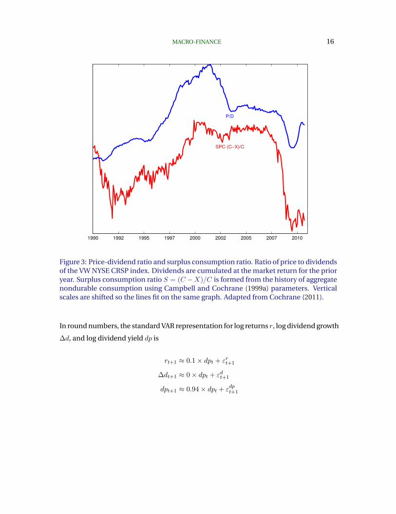
Recent history. How does the model perform since publication? The model says that

the price-dividend ratio should track the surplus consumption ratio. Figure 3 plots

the price-dividend ratio and surplus-consumption ratio, inferred from the history of

nondurable consumption.

As you can see, the brickbats thrown at modern finance for being utterly unable to

accommodate the financial crisis are simply false. Consumption relative to habit rises

in the pre-crisis boom, and falls at the same time as stock price/dividend ratios fall. The

model works better in big events.

Now, for some directions needing improvement. The model has quite a few flaws. Most

of these flaws are common to alternative frameworks. We expected an active literature

that would improve it along these dimensions. That hasn’t happened yet, but perhaps I

can inspire some readers to try.

More shocks. The consumption-claim version of the habit model has one shock, the

shock to consumption growth. This shock is simultaneously a cashflow shock and a

discount rate shock, so the cashflow and discount rate shocks are perfectly negatively

correlated. When consumption declines (cashflow shock), the discount rate rises.

The standard VAR representation of returns and dividend yields has at least two distinct

shocks. In the simplest VAR, cashflow shocks and discount rate shocks are uncorre-

lated.

MACRO-FINANCE 16

1990 1992 1995 1997 2000 2002 2005 2007 2010

SPC (C−X)/C

P/D

Figure 3: Price-dividend ratio and surplus consumption ratio. Ratio of price to dividendsof the VW NYSE CRSP index. Dividends are cumulated at the market return for the prioryear. Surplus consumption ratio S = (C −X)/C is formed from the history of aggregatenondurable consumption using Campbell and Cochrane (1999a) parameters. Verticalscales are shifted so the lines fit on the same graph. Adapted from Cochrane (2011).

In round numbers, the standard VAR representation for log returns r, log dividend growth

∆d, and log dividend yield dp is

rt+1 ≈ 0.1× dpt + εrt+1

∆dt+1 ≈ 0× dpt + εdt+1

dpt+1 ≈ 0.94× dpt + εdpt+1

MACRO-FINANCE 17

and the covariance matrix of the shocks is

cov(εε′) =

r ∆d dp

r σ = 20% +big -big

∆d σ = 14% 0 not -1

dp σ = 15%

The definition of return means that only two of the three equations are needed, and the

other one follows. If prices rise or dividends rise, returns must rise. In equations, the

Campbell-Shiller return approximation is

rt+1 ≈ dpt − ρdpt+1 + ∆dt+1

where ρ ≈ 0.96 is a constant of approximation. (This equation is just a loglinearization

of the definition of a return,Rt+1 = (Pt+1 +Dt+1)/Pt. As a result of this identity, the VAR

regression coefficients b and shocks ε are linked by identities

br = 1− ρbdp + bd

εrt+1 = −ρεdpt+1 + εdt+1

With any two coefficients, shocks, or data series, you can find the last one.

It is common to write the VAR with dividend yields and returns, {dpt, rt} and let dividend

growth be the implied variable. I like to think of it instead in terms of dividend growth

and dividend yields {dpt,∆dt} with returns the implied variable. (“Think of it,” but

don’t run it that way. Never run a return forecasting regression with less than a pure

return. Small approximation errors can make returns look much more forecastable than

they really are.) The reason for this preference is that, while dp and r shocks are very

negatively correlated – when prices go up, dividend yields go down and returns go up –

MACRO-FINANCE 18

dp and ∆d shocks are essentially uncorrelated.

Thus, the easy-to-remember summary of the canonical three-variable VAR is this: There

are two shocks in the data: a cashflow shock εd, and a discount rate shock εdp, and

these two shocks are uncorrelated. The negative correlation of return and dividend yield

shocks εr, εdp, and the positive correlation of return and dividend growth shocks εd, εr

then just follows from the last identity.

Clearly, this little VAR paints a different picture than our consumption-claim model in

which the cashflow and discount rate shocks are perfectly correlated. We need to think

of a world with separate and uncorrelated cash-flow and discount-rate shocks, at least

when using the dividend yield alone to capture conditioning information.

Campbell and Cochrane (1999a) includes a model with a claim to dividends poorly cor-

related with consumption, which makes progress towards a two-shock model. Even that

model does not replicate the VAR, however.

Cointegration. And it suffers from another problem: Consumption, stock market value,

and dividends are cointegrated. Consumption and dividends are both steady shares of

GDP in the long run. The paper just specifies imperfectly correlated growth rates of

consumption and dividends ∆c and ∆d. But the levels of consumption and dividends

wander away from each other.

Many models have imperfectly correlated ∆c and ∆d. I have not seen one yet that

properly delivers the long run stability of the ratios of stock market value, consumption,

and dividends.

Cointegration is tricky. Total dividends and total consumption are cointegrated. The

usual measure of dividends one recovers from asset pricing data is dividends accruing

to an initial dollar investment. These are different concepts, and the latter is not cointe-

grated with consumption.

More state variables? The habit model has one state variable, the surplus consumption

MACRO-FINANCE 19

ratio St = (Ct − Xt)/Ct. The dividend yield is perfectly revealing of this state variable,

so no other variable should help to forecast stock returns, bond returns, volatility, or

anything else. And all variables that are a function of this state variable should be per-

fectly correlated, as the surplus consumption ratio and price-dividend ratio should be

perfectly correlated. Conditional variances move over time, and the conditional Sharpe

ratio moves over time as well, becauseE(Ret+1|St) and σ(Ret+1|St) are different functions

of the state variable St. The version the habit model that allows for time-varying inter-

est rates, Campbell and Cochrane (1999b), also has time-varying bond risk premiums

forecast by yield spreads. But all of these variables are are functions of the same state

variable, so perfectly correlated with dividend yields and with each other.

In the empirical literature, many variables beyond the dividend yield seem to forecast

both stock returns and dividend growth. The Lettau and Ludvigson (2001) consumption

to wealth ratio cay is a good example, which I examine in some depth in Cochrane

(2011). In the cross-section of returns, size, book-market, momentum, earnings quality

and now literally hundreds of other variables are said to forecast returns. Harvey, Liu,

and Zhu (2016) list 316 variables in the published literature! Bond returns are fore-

castable by bond forward-spot spreads, and foreign exchange returns by international

interest spreads.

Now, a big empirical question remains: Just how many of these state variables do we

really need, in a multiple regression sense? The forecasting variables are correlated with

each other. Are they all proxies for a single underlying state variable? Or maybe two or

three state variables, not hundreds?

The question is, what is the factor structure of expected returns? If we run regressions

Reit+1 = ai + bixt + ciyt + ..εit+1; Et(Reit+1) = ai + bixt + ciyt,

how many state variables – orthogonal linear combinations of x, y, z – do we really need?

What is the factor structure of cov[Et(R

eit+1)

]? Look at that question closely – this is not

MACRO-FINANCE 20

the factor structure of returns, cov(Reit+1

), time t + 1 random variables. It is the factor

structure of expected returns, time t random variables. This covariance and its factor

structure may have nothing to do with the factor structure of ex-post returns. But what

is that factor structure? Across stocks, bonds, foreign exchange etc.? As a small first step,

Cochrane and Piazzesi (2005) and Cochrane and Piazzesi (2008) find that the covari-

ance of bond expected returns across maturities has one dominant factor. Does that

observation extend to bonds and stocks? Probably not. But the bond-forecasting factor

forecasts stocks, and dividend yields forecast bonds, so there is some commonality. How

much of a second factor do we really need? Bringing some order to the zoo of factors that

forecast the cross-section of stock returns is even more important – I hope we don’t need

300 separate factors.

Conditional variances σt(Rt+1) vary over time as well. The empirical literature seems to

focus on realized volatility – lagged squared returns – and volatilities implied by options

prices as the state variable for variance. These variables decay much more quickly than

typical expected return forecasters like dividend yield. Realized volatility also forecasts

mean returns, though, and dividend yields forecast volatility. How many state variables

are there really driving means and variances?

Finding the factor structure across assets and asset classes of conditional moments (mean

and variance), and seeing how many different forecasters we really need, is a big and

largely unexplored empirical project.

The answer is unlikely to be one factor, as specified in the habit model. Hence, the nat-

ural generalization of theory must be to include more state variables, to match the more

state variables in the data. Wachter (2006) has taken a step in this direction, separating

somewhat bond and stock forecasts, but there is a long way to go.

Finally, there is a flurry of work now looking at the term structure of risk premiums,

which may provide a new set of facts for models to digest. In simplest form, this work

distinguishes EtRt+k across different horizons k. In my evaluation the empirical facts

MACRO-FINANCE 21

of this literature are still tenuous for solid model fitting, but the direction of research is

worth noting.

Tests. Habit models really have not been subject to much formal testing. (Tallarini and

Zhang 2005 is a lonely counter-example.)

Of course, as we are learning with the second generation of consumption-based model

tests, glasses can be a lot more full than we thought. Many of the early consumption

model rejections used monthly, seasonally adjusted, time-aggregated consumption data.

No surprise that didn’t work. More recent tests, such as Jagannathan and Wang (2007),

use of fourth quarter to fourth quarter annual data, find unexpected success for the con-

sumption based model. Campbell and Cochrane (1999a) and Campbell and Cochrane

(2000) also show how time-aggregation can destroy model predictions.

So we’re still waiting for a really good assessment of the power utility based consumption

based model, alone, as well as with habit and other novel preferences, but doing its best

to see where the glass is half or more full, by treating carefully durability (nondurable

consumption includes clothes for example), seasonality, time aggregation, data collec-

tion issues, and so forth.

In general, since the classic consumption-based model tests in the early 1980s, eco-

nomics and finance have moved away from formal testing – can we tell that this model is

not exactly true? – to less formal evaluation of just how much the model can illuminate

data, and where its economically significant failures lie. All models can be rejected with

enough data. And many models that can be rejected as absolute truth are quite useful

anyway. For example, the Fama and French three-factor model is far and away the most

important and practically useful asset pricing model of the last quarter century. And it

is blown away by formal GRS test statistics. It is easy to formally reject models, to prove

that they are not 100% accurate, while not noting that they provide very good accounts

of the central and robust phenomena. It is easy to fail to reject models that provide no

useful account of the data at all.

MACRO-FINANCE 22

Like all explicit general equilibrium models, the habit model can swiftly be rejected.

All explicit economic models have R2 = 1 predictions in them somewhere, unless the

researcher salts them up with shocks to each equilibrium condition or measurement

errors. The permanent income model says that consumption is the present value of

future income, with no error term. If you add a model for income, a combination of

consumption and income state variables has no error. The Q theory of investment

says that investment equals a function of stock prices, with no error term. The habit

model says that the dividend yield is nonstochastic function of the surplus consumption

ratio. A graph such as Figure 3 is a 100% probability rejection of the model, because the

consumption and stock price lines are not exactly on top of each other. So the real art

of testing is to see in what sensible predictions of a model are really at odds with the

data, avoiding “rejecting” a model because a 100% R2 prediction is only 99.9% in the

data.

These deficiencies are common to all macro-asset pricing models. There is lots of low-

hanging fruit in this business! For the moment though, the literature has focused on the

parallel development of alternative preferences and market structures.

2.3. Recursive utility and long-run risk

The recursive utility approach uses a nonlinear aggregator to unite present utility and

future value,

Ut =

((1− β)C1−ρ

t + β[Et

(U1−γt+1

)] 1−ρ1−γ) 1

1−ρ

. (3)

Here γ is the risk aversion coefficient and 1/ρ is the elasticity of intertemporal substitu-

tion. This function reduces to time-separable power utility for ρ = γ.

MACRO-FINANCE 23

The discount factor, or growth in marginal utility, is

Mt+1 = β

(Ct+1

Ct

)−ρ Ut+1[Et

(U1−γt+1

)] 11−γ

ρ−γ

= β

(Ct+1

Ct

)−ρ(Yt+1)ρ−γ .

In the latter equation, I emphasize that the innovation in the utility index takes the role

of the new variable Y in my general classification.

The utility index itself is not observe, so the trick is to substitute for it in terms of ob-

servable variables. Though Epstein and Zin (1989) used the market return, the most

common approach recently, exemplified by Bansal, Kiku, and Yaron (2012), and Hansen,

Heaton, and Li (2008), is to substitute the utility index for the stream of consumptions

that generate utility. This substitution delivers the long run risk model. For ρ ≈ 1,

∆Et+1 (lnMt+1) ≈ −γ∆Et+1 (∆ct+1) + (1− γ)

∞∑j=1

βj∆Et+1 (∆ct+1+j)

where ∆Et+1 ≡ Et+1 − Et.

In this formulation, news about long run future consumption growth is the extra state

variable Yt. As usual this extra state variable does the bulk of the work to explain risk

premiums. Here, people are afraid of stocks that might go down when there is bad

news about long-run future consumption growth, not necessarily when the economy

is currently in a recession, or a time when consumption is low relative to its recent

past.

This model is very popular. Still, I think there is room to question the wisdom of this

popularity.

First, the model crucially needs there to be news about long run consumption growth –

MACRO-FINANCE 24

variation in ∆Et+1∆ct+j , j > 1 – to get anywhere. If consumption is a random walk; if

day by day consumers answer a hypothetical survey about their expectations of con-

sumption growth in 2030 with the same number, say 1%, then there is no long-run

consumption news and the model reduces to time-separable power utility.

Current conditions ∆ct are essentially irrelevant to investor’s fear. Investors only seem to

fear stocks that go down when current consumption goes down (fall 2008, say) because,

by coincidence, current consumption declines are correlated with the bad news about

far-off long-run future consumption growth that investors really care about.

So is there a lot of news about long-run consumption growth? And is it at all believable

that this is really what investors care about? The former is hard to find in the data. Apart

from a first-order autocorrelation due to the Working effect (a time-averaged random

walk follows an MA(1) with an 0.25 coefficient) and the effects of seasonal adjustment

(our data is passed through a 7 year, two-sided bandpass filter), nondurable and services

consumption looks awfully close to a random walk. (Beeler and Campbell 2012 elabo-

rate this point.) Inferring long-run predictability from a few short-run correlations is a

dubious business in the first place. Maximum likelihood and related econometric tech-

niques value short-run forecasts, and are happy to get long-run forecasts wrong, or to

miss many high-order autocorrelations, in order to better fit one-step ahead predictions

(Cochrane 1988.)

One might retort, well, the standard errors are big, so you can’t prove there isn’t a lot

of long-run positive autocorrelation in consumption growth. But demoting the central

ingredient of the model from a robust feature of the data to an assumption that is hard

to falsify clearly weakens the whole business.

I often advise students to write the op-ed or teaching note version of their paper. If you

can’t explain the central idea to a lay audience in 900 words, then maybe it isn’t such a

good idea after all.

In this case, that oped would go something like this: Why were people so unhappy with

MACRO-FINANCE 25

their decision to hold stocks in, say, fall 2008? It was not, really, because the economy

was in a recession, that investors had lost their jobs and houses and they were cutting

back on consumption. Those facts, per se, were irrelevant. Instead, it was because

2008 came with bad news about the long-run future. Investors figured out what no

professional forecaster did, that we would enter these decades of low growth. If that bad

news about long-run growth happened to be correlated with a boom in 2008, people

would have paid dearly ex ante to avoid stocks that did particularly badly in the boom.

People, and the institutions such as university endowments trying to sell in a panic,

didn’t fundamentally care at all about what was happening in 2008 – it’s only the long

run news that mattered to them.

This strikes me as a difficult essay to write, and a difficult proposition to explain honestly

to an MBA class on any day but the first of April.

To understand the long-run risk model, ask this (a good exam question): How is the

long-run risk model different from Merton’s ICAPM? After all, the ICAPM also includes

additional pricing factors, that are “state variables for investment opportunities.” News

about long-run consumption growth would certainly qualify as an ICAPM state variable.

Yet the ICAPM has power utility. Why did we need recursive utility to get long-run

consumption growth expectations to matter for asset prices?

The answer is that the ICAPM is a subset of the power-utility consumption-based model.

Its multiple factors are the market return and state variables, not consumption growth

and state variables. In response to bad news about future consumption, ICAPM con-

sumers reduce consumption today. That reduction in today’s consumption reveals all

we need to know about how much the bad news hurts.

By contrast, the long-run risks model weights news about future consumption that is

not reflected in consumption today. Somehow, you get news that you will be poor in the

future. You rue the decision to buy stocks, yet still choose to consume a lot today. This

is the kind of bad news about which you are really afraid. If you did react by lowering

MACRO-FINANCE 26

consumption today then today’s consumption would be a sufficient statistic for the bad

long run news, and that news would have no extra explanatory power.

In the habit model, people really are worried about stocks falling in 2008 – because of

events going on in 2008. The fall in consumption to the minimum tolerable level they

have gotten used to in the previous decade is what makes them regret having bought

stocks; and the consequent greater fear of further falls in consumption – widespread in

2008 – induces them to try to sell despite high expected returns going forward.

Fear of news about the far off future, unrelated except by coincidence and correlation to

macroeconomic events today, is closely related to the central theoretical advertisement

for recursive utility. Recursive utility captures – and requires – a “preference for early

resolution of uncertainty.” This is a tricky concept. In almost all of your experience you

prefer to resolve uncertainty early because you can do something with that knowledge.

If you know what your salary will be next year, you can start looking for a better house,

or a better job. If you learn what the stock market will do next year, you can buy today.

The preference for early resolution of uncertainty that these preferences capture is a

pure pleasure of knowing the future, even when you can’t do anything in response to the

news.

I find lab experiments documenting such preference unpersuasive, because there is es-

sentially no circumstance in daily life in which one gets news that one can do absolutely

nothing about. People respond to surveys and experiments with rules of thumb adapted

to the circumstances of their lives.

Epstein, Farhi, and Strzalecki (2014) address the question this way: How much would

the consumer in the Bansal-Yaron economy pay, by accepting a lower overall level of

consumption, in order to know in advance what that consumption will be? The answer

is around 20 to 30 percent – the consumer would accept a stream that is 20 to 30 percent

lower on every single day of his or her life, just for the psychic pleasure of knowing what

it will be in advance. That seems like a lot.

MACRO-FINANCE 27

Genetic testing for Huntington’s disease is one real-world circumstance that almost fits

the model. There is no cure, you simply find out if you’re going to get the disease. In

this case there is quite a bit one can do with the information, such as make career,

family, investment, and estate decisions. Nonetheless, Oster, Shoulson, and Dorsey

(2013) point out that few people with family history get the test.

So, capturing a strong preference for early resolution of uncertainty starts to me to look

more like a bug than a feature.

This isn’t some sideline technical issue – it’s central to the whole long-run risks idea. The

news about future consumption, unrelated to current consumption, that so drives risk

premiums in the model, is exactly this psychic pleasure or pain of learning the future,

unrelated to current action or any planning, investing, or other actions one can take in

regard to the news. If you don’t believe one, you don’t believe the other.

The other apparent theoretical advantage is that recursive utility separates risk aversion

from intertemporal substitution, allowing high risk aversion for the equity premium and

a low and steady risk free rate.

But so do habits. The habit model delicately offsets time-varying intertemporal sub-

stitution demands with a time-varying precautionary saving and thereby generates the

same result.

I grant that recursive utility achieves the result more elegantly, and that elegance and

tractability are important in economic theories. But that elegance and tractability may

lead us astray. If in fact time-varying precautionary saving is important – if, say, Fall

2008 had a large fall in consumption because people were scared to death – then the

model is missing the crucial feature of reality. Furthermore, though the square root habit

adjustment process in our model is inelegant, it requires much less algebra than one

must surmount to solve recursive utility models.

The recursive utility model, like the habit model, produces the equity premium with a

MACRO-FINANCE 28

low and stable risk free rate and realistic (low) one-period consumption volatility. It can

use high risk aversion, as in the habit model. It can also produce the equity premium

with relatively low risk aversion, by imagining a lot of positive serial correlation in con-

sumption growth – a lot of long-run news. In this case, though, long run consumption

volatility is very high, so it is in the class of theories that abandon the low consumption

volatility ingredient of the equity premium puzzle statement. (E(Re)/σ(Re) = γσ(∆c)

can be achieved with high ∆c.)

Return predictability and time-varying volatility are the more interesting and challeng-

ing, phenomena, and the ones more tied to macroeconomics. The long-run risk model

does not endogenously produce time-varying risk premia. These are added by assum-

ing an exogenous pattern of consumption volatility. This explanation of predictability

goes back to Kandel and Stambaugh (1990) with power utility: To get Et(Re)/σt(Re) ≈

γσt(∆ct+1) to vary over time with constant γ, you need to imagine that σt(∆ct+1) varies

over time.

Again there is little direct evidence for the proposition that the conditional variance

of consumption growth varies significantly over time and is tightly correlated to price-

dividend ratios. Moreover, it’s a second exogenous coincidence. The habit model builds

in a time-varying Sharpe ratio, higher in bad times, endogenously. Risk aversion γ rises

as consumption falls towards habit.

So, the interesting predictions of the model have to be baked in by the assumptions

on the exogenous consumption process – serial correlation of consumption growth, so

that today’s consumption fall signals a large long run risk, and time-varying volatility

of consumption so that today’s consumption fall is correlated with a higher expected

return. As a result, the predictions are very sensitive to those auxiliary assumptions.

And there is little clear direct support for those assumptions in data. This sensitivity

raises the question whether in a production and investment economy, consumers will

choose a consumption process with just the right correlation of short-run and long-run

risks, and the variation in volatility, needed to produce the large asset pricing swings we

MACRO-FINANCE 29

observe.

To progress, all extra state-variable models need to propose some independent way of

measuring shifts in marginal utility, and that measurement should contain as few extra

assumptions as possible. In the habit model, the extra state variable – surplus consump-

tion ratio – is directly and independently measurable. Furthermore, the model generates

the extra state variable – surplus consumption ratio – endogenously via the link between

consumption and habit.

The Bansal and Yaron (2004) long run risk model ties its dark matter – news about long

run consumption growth – to observables by the assumption that short-run consump-

tion growth is correlated with to volatility and long-run news. That assumption makes

long-run news independently measurable. But the crucial link is driven by extra as-

sumptions about the exogenous driving process, not the economic structure of the model.

Finally, substituting the market return or long-run consumption growth for the utility

index in (3) requires that we use the entire wealth portfolio (claim to total consumption

stream) or total consumption. The usual trick in separable utility, that the asset pricing

implications of u(cnd) + v(cd) are the same as those of u(cnd) alone, where cnd and cd

represent consumption of nondurables and durables respectively, does not work for

nonseparable utility. There seems to be a gentleman’s agreement not to worry about

this fact.

However, the habit and recursive utility models have a lot in common, and that com-

monality is my greater theme. Both models capture a quite similar idea. There is an

extra state variable, which explains why people are afraid of holding stocks in ways not

described by just consumption growth. That extra state variable has something to do

with recessions, bad macroeconomic times. Both models capture an equity premium

and time-varying predictability, one with time-varying risk, the other with time-varying

risk aversion. No model has gotten significantly ahead of the others in terms of the

number of phenomena it captures. All models have inconvenient truths that we ignore,

MACRO-FINANCE 30

as the original CAPM required no investor to hold a job, and predicted that consumption

volatility is the same as market volatility. That didn’t stop it from being a useful model for

many years. The habit model carefully reverse-engineers preferences to deliver the eq-

uity premium and predictability. The long-run risks model carefully reverse-engineers

the exogenous consumption process to deliver the same phenomena. One observer’s

“fragile” assumption is another observer’s “well-identified” parameter. Though I have

argued that model-derived assumptions are prettier than driving-process assumptions,

that is an esthetic judgment.

(Equations: The Bansal, Kiku, and Yaron 2012 consumption process is

∆ct+1 = µc + xt + σtηt+1

xt+1 = ρxt + φeσtet+1

σ2t+1 = σ2 + v(σ2

t − σ2) + σwwt+1

∆dt+1 = µd + φxt + πσtηt+1 + φσtud,t+1

The x process generates positive serial correlation in consumption growth, so that small

changes build up over time. σt gives the time-varying risk which drives time-varying

expected returns.)

2.4. Idiosyncratic risk

Idiosyncratic risk, such as in Constantinides and Duffie (1996), is another fundamentally

different microeconomic story that generates similar results.

The bottom line is again a discount factor that adds a state variable to consumption

growth,

Mt+1 = β

(Ct+1

Ct

)−γ (eγ(γ+1)

2y2t+1

).

Here yt+1 denotes the cross-sectional variance of consumption growth. The log of each

MACRO-FINANCE 31

individual’s consumption follows

∆cit+1 = ∆ct+1 + ηi,t+1yt+1 −1

2y2t+1; σ2 (ηi,t+1) = 1

Therefore, yt+1 plays the role of the second, recession-related state variable in place of

the surplus consumption ratio or long-run risk.

The story: People are afraid that stocks might go down at a time when they face a lot

of idiosyncratic risk. Some might get great gains, some might face great losses. With

risk aversion, i.e. nonlinear marginal utility, fear of the losses outweighs pleasure at the

gains, so overall people fear assets that do badly at times of great idiosyncratic risk.

The Constantinides and Duffie paper is brilliant because it is so simple, and it provides

directions by which you can reverse-engineer any asset pricing results you want. Just

assume the desired cross-sectional variance yt+1 process. This reverse engineering also

circumvents many problems with the previous idiosyncratic risk literature.

As with the long-run risks model, however, the level and especially the time-variation

and business cycle correlation of the equity premium all are baked in by the exogenous

variation in the moments of the income process, rather than the endogenous response

of risk aversion to bad times. Cross-sectional consumption volatility must be large, and

must vary a good deal over time, and at just the right times.

One can check the facts, and so far the empirical work has been a bit disappointing to

the model. Cross-sectional risks do rise in recessions, and when asset prices are low, but

they do not seem large enough, or time-varying enough to generate the asset pricing

phenomena we see at least with low levels of risk aversion. Consumption risks are much

smaller than transitory income or employment risks. However, this is still an active area

of empirical research. For example, Schmidt (2015) has recently investigated whether

the non-normality of idiosyncratic risks can help – whether a time-varying probability

of an idiosyncratic rare disaster dominates the cross-sectional risks to marginal utility.

Such events are intuitively plausible.

MACRO-FINANCE 32

Again you can see the essential unity of the ideas. A second state variable, associated

with recessions, drives marginal utility. People are afraid that stocks might fall in re-

cessions, and being in a recession and a time of low-price dividend ratios raises that

fear. Here “recessions” are measured by a large increase in idiosyncratic risk, rather

than by a fall of average consumption relative to its recent past. But those events are

highly correlated. In the habit model, the second state variable is endogenous, and

tied directly to the fall in consumption, rather than exogenous and requiring an extra

set of assumptions. But that is minor. The moments of cross-sectional risk are at least

more tightly tied to data and measurable than the inference about long-run risk from

its correlation with short run risks. And they are much more restricted and measurable

than the extra state variables in long-run risks and psychological models to come.

2.5. Heterogeneous preferences

Garleanu and Panageas (2015) offer a related but diametrically opposed model. For Con-

stantinides and Duffie, people have the same preferences, risks are not insured across

people, and exposure to this time-varying cross-sectional risk drives asset prices. For

Garleanu and Panageas, people have different preferences. Some are more risk averse,

and some are less risk averse. Risks are perfectly insured across people. Now, less risk

averse people hold more stock than more risk averse people. But, when the market goes

down, these big stockholders lose more money, and so they become a smaller part of the

overall market. So, by shifting consumption from the risk-takers to the risk-haters, the

market as a whole becomes more risk averse after a fall in value.

More precisely, in a complete market the unique discount factor Λt and consumer A, B

consumption follow

Λt = e−δtC−γaA,t = e−δtC−γbB,t

Thus in bad times, with high Λt, the less risk averse consumer accepts greater consump-

MACRO-FINANCE 33

tion losses, while in good times, that consumer enjoys greater gains. Mechanically, this

sensitivity is implemented via greater investment in the market.

Differentiating these relationships, we can express the discount factor in terms of ag-

gregate consumption Ct = CA,t + CB,t raised to an aggregate risk aversion, which is the

consumption - weighted average of individual’s inverse risk aversion.

1

γmt=

1

γB

CB,tCt

+1

γA

CAtCt

.

You see here exactly the sort of mechanism of a habit model – the representative agent

becomes more risk averse after a fall in consumption. But here, that rise does not come

because each individual becomes more risk averse. It comes because the mechanism

of aggregation puts more weight on the risk averse people in bad times.

This is a beautiful model, which emphasizes just how many micro stories are consistent

with the same macro phenomenon. The representative consumer has time-varying risk

aversion though individuals do not. Markets display less risk bearing capacity in bad

times. That phenomenon can be driven by market structures as well as by psychology of

individual preferences.

This model faces challenges in the micro data just as the idiosyncratic risk model does.

Do the “high-beta rich” really lose so much in bad times? But that investigation hasn’t

really started.

2.6. Debt, balance sheets, and institutional finance

A different category of model has become much more popular since the 2008 financial

crisis: models involving debt, balance sheets, mortgage overhang; institutional or inter-

mediated finance.

The basic story works much like habit persistence. Imagine that an investor has taken

MACRO-FINANCE 34

on a level of debt X, which he or she must repay. Now, as income declines towards X,

the investor will take on less and less risk, to make sure that even in bad states of the

world he or she can repay the debt. The intuition of Figure 1 applies exactly, if we just

re-label X as the level of debt.

Moreover, as consumption rises in good times, people slowly take on more debt. As

consumption falls in bad times, people “delever,” “repair balance sheets” and so forth.

So debt moves slowly, following consumption, much like slow-moving habit.

Though the mechanism is broadly similar, however, debt-based finance models are deeply

different from all the others in this survey. In all the other models, even psychological

ones, markets function fairly well in equating margins between borrowers and lenders.

Asset price variations result from preferences or perceptions of each individual. (Be-

havioral models have some frictions on occasion to keep arbitrageurs from removing

pricing errors, but the source of pricing errors remains misperceptions by each individ-

ual.) In intermediated-finance models, by contrast, market failures are central to the

story. In this story, for example, the vast bulk of people did not change risk preferences

or probability mis-perceptions in 2008. They would have loved to have bought at fire-

sale prices. But they were not “marginal,” for some reason unable or unwilling to buy

cheaply priced stocks directly. Only the newly-risk averse leveraged intermediaries were

active in markets. Similarly, households and businesses would have loved to borrow

more to finance purchases or investment, but leverage and capital constraints at banks

stopped money from flowing from willing lenders to willing borrowers.

As attractive as some of the stories may be, however, these models also face some diffi-

culties.

First, why do agents get more risk averse as they approach bankruptcy, not less? Bankruptcy

is the point at which you don’t have to pay your debts any more. It is usually modeled

as a call option. Debt in our economy is not an absolute requirement to pay, with failure

to pay resulting in debtors’ prison, destitution, or worse. The usual concern is therefore

MACRO-FINANCE 35

that people and businesses near bankruptcy have incentives to take too much risk, not

too little. If the bet wins, you’re out of trouble. If the bet loses, the bank or creditors take

bigger losses – not your problem.

The costs, benefits, reputational concerns, and so forth surrounding bankruptcy are

subtle, of course, and I don’t mean to argue that we know exactly one way or another in

all circumstances. I do point out that it’s not at all obvious that debt should induce more

risk aversion rather than less, and it takes modeling effort and dubious assumptions to

produce the more answer.

Second, not everyone is in debt. My debt is your asset – net debt is zero. For this

reason, institutional finance models center on segmented markets, so that the problems

of borrowers weigh more heavily on markets than the problems of their creditors.

The typical institutional finance story told of the financial crisis goes like this: Funda-

mental investors – you and me – give our money to intermediaries. The intermediaries

take on leverage, so we split our funding of the intermediaries into debt and equity

tranches. When the intermediaries start losing money, they get more risk averse, and

start selling assets. (For various reasons they don’t raise more equity, give us securities,

or bet the farm on riskier trades.) You and I don’t trade in the underlying assets, so there

is nobody around to sell to. Only the intermediaries are “marginal.” Hence, when they

try to sell, prices go down. That puts them closer to bankruptcy, so they sell more, with

colorful names like “liquidity spiral,” or “fire sale.”

The objections to this sort of model are straightforward. OK, for obscure CDS or other

hard to trade instruments, and this may explain why small arbitrages opened up be-

tween more obscure derivatives and more commonly traded fundamentals. But how

does this story explain widespread, coordinated, long-lasting movements in stock and

bond markets around the world? After all, these assets are part of everybody’s pension

funds. We’re all “marginal,” at least at the month to years horizons over which business

cycles evolves.

MACRO-FINANCE 36

Moreover, large, sophisticated, unconstrained, debt-free wealthy investors and institu-

tions such as university endowments, family offices, sovereign wealth funds, and pen-

sion funds all trade stock indices and corporate bonds every day. If leveraged interme-

diaries push these prices down nothing stops these investors from buying. Where were

they in the crisis? Answer: they were selling in a panic like everyone else. That surely

smacks of time-varying risk aversion, induced by recent losses, not a segmented market

in which fundamental investors want to buy but leverage and agency problems cause

their agents to sell.

Furthermore, if there is such an extreme agency problem, that delegated managers were

selling during the buying opportunity of a generation, why do fundamental investors

put up with it? Why not invest directly, or find a better contract?

To be clear, I think the evidence is compelling that “small” arbitrage opportunities in

hard-to-trade markets during the fall of 2008 were linked to intermediary problems. I

put “small” in quotes, because an economically small arbitrage opportunity – say, a 1%

deviation from covered interest parity – while not enough to attract long-only interest

on one side or the other, represents a potentially enormous profit for a highly leveraged

arbitrageur. Still, a 1% price deviation is still small from the perspective of the overall

economy.

But the presence of those frictions and arbitrages does not mean that leveraged interme-

diaries are responsible for the bulk of the large movements in stocks, bonds, government

bonds, and foreign exchange that we saw during the crisis. Their presence means even

less that perpetually constrained, leveraged intermediaries and absent fundamental in-

vestors are always the story for financial market movements, continuing to this day.

Inequality constraints don’t bind when they’re slack, and people who run in to them

take care not to have them bind forever.

Business and consumer debt, “leveraging” and “deleveraging” or “balance sheets” are an

attractive alternative mechanism for inducing time-varying risk aversion. The models

MACRO-FINANCE 37

also can look a lot like a habit model. But I have similar doubts about the view that

business and consumer debt is the major driver of asset prices and macroeconomics,

rather than contributing relatively minor, if important, epicycles. If bad times mean

that the consumer will be close to the default limit, then why borrow so much in the first

place? Buffer stock models require very high discount rates to eliminate this natural ten-

dency to save up enough assets to avoid the bankruptcy constraint Though the average

person may be constrained, the average dollar driving the risk-bearing capacity of the

market is held by an unconstrained consumer. As the heterogeneous agent literature

reminds us, the market risk tolerance is the wealth weighted average of individual risk

tolerance.

The institutional finance view also does not easily explain why asset prices are so related

to macroeconomic events. Losing money on intermediated and obscure securities is

not naturally related to recessions. The 2007 hedge fund collapse did not lead to a

recession.

One might imagine reverse causality, a new model of macroeconomics by which finan-

cial events spread to the real economy not vice versa. That’s an exciting possibility, ac-

tually, and the core of the bustling frictions-based macro-finance research agenda. But

at this stage it’s really no more than a vision – models adduce frictions far beyond reality,

such as that no agent can buy stocks directly, and data analysis of one event.

So, in my view, institutional finance and small arbitrages are surely important frosting

on the macro-finance cake, needed to get a complete description of financial markets

in times of crisis. But are they also the cake? And are they the meat and potatoes and

vegetables of normal times, and the bulk of movements in broad market indices, and

the explanation for their correlation with macroeconomics? Or can we understand the

big picture of macro-finance without widespread frictions, and leave the frictions to

understand the smaller puzzles, much as we conventionally leave the last 10 basis points

to market microstructure, but do not feel that microstructure issues drive the large busi-

ness cycle movements in broad indices?

MACRO-FINANCE 38

Again, though, my main point is to point out the many commonalities, and only slightly

to complain about differences. Theories based on debt deliver the same central idea,

that the risk bearing capacity of the market declines in bad times.

The theories outlined so far differ mainly in the exact state variable for expected re-

turns – consumption relative to recent values, news about long-run future consumption,

cross-sectional risk, or leverage; balance sheets of individual consumers or those of

leveraged intermediaries. But all four state variables are highly correlated, and all four

capture the idea that investors are scared of recessions.

2.7. Rare disasters

Barro (2006) has recently taken up an idea of Reitz (1988), that the equity premium and

other asset pricing phenomena can be understood by the fear of rare disasters. With

Barro’s inspiration, this idea has expanded substantially.

Look back at the basic asset pricing equation,

Et(Ret+1) = covt

[(Ct+1

Ct

)−γ, Ret+1

]≤ σt

[(Ct+1

Ct

)−γ]σt(Ret+1

).

If people worry about rare events with very low consumption growth, then the variance

of marginal utility in investors heads will be larger than the variance we measure in a

sample that doesn’t include any rare events.

The basic idea is reasonable, that people worry about rare and severe events when buy-

ing securities. People in California still worry about large earthquakes, though we haven’t

seen one since 1906, and rare events are priced in to earthquake insurance.

To get rare disasters to account for the more interesting and business-cycle related re-

turn predictability and stock price volatility, one could specify that the risk of a rare

consumption or return disaster changes over time – that σt[(ct+1/ct)−γ or σt(Rt+1) vary

MACRO-FINANCE 39

over time, due to changing tail probabilities.

Alternatively, a rare-disasters perspective could posit that expected returns really do not

change over time. People see time-varying probabilities of a rare disaster in dividend

payouts. Prices really are lower because expected dividends are lower, not because ex-

pected returns are higher. But in a sample that has no rare disasters we suffer Peso-

problem regressions that falsely indicate return predictability rather than dividend pre-

dictability, and consequently falsely indicate “excess” volatility.

One objection to this view is that we should have seen more disasters if they are large

or frequent enough to account quantitatively for the equity premium with low risk aver-

sion. This observation has led much work quantifying just how many disasters we have

seen, in the US and abroad, over long spans of time, how to define a disaster, and what

it constitutes. (Events in which both stocks and bonds become worthless don’t justify an

equity premium.) Calibration of time-varying rare disaster models to account for pre-

dictability and volatility is still in its infancy. (Welch 2016 also finds that the probabilities

of rare disasters implied by put option prices are far too low to account for much of the

equity premium.)

Dark matter is a deeper objection. Unobserved rare events are already to some ex-

tent a dark matter assumption. But to get the central phenomena of macro-finance –

return predictability, price/dividend ratio volatility, varying volatility, all of this corre-

lated with business cycles – we need time-varying probabilities of rare disasters. That

seems like dark energy (i.e. even more obscure) – unless one proposes some way of

independently tying the time-varying probability of rare disasters to some data. One

might surmount the dark-matter criticism if one assumption about time-varying disas-

ter probability could reconcile multiple asset prices, but as Gabaix (2012) has pointed

out, to make sense of the different asset classes, one needs to assume a asset-specific

time-varying loading on the disaster risk.

Finally, the correlation of asset prices with business cycles relies on a correlation of

MACRO-FINANCE 40

business cycles with a time-varying disaster probability. As a correlation between short-

run consumption growth and long run news is not totally implausible, neither is this

correlation. But it is one more exogenous assumption, and one step harder to test than

the correlation of consumption growth with long-run news.

In sum, the rare disaster view also requires a complex set of assumptions about the

exogenous endowment process in order to explain the appearance of time-varying risk

premia. Like the long-run risks model, measuring this process independently is chal-

lenging.

I admit a final prejudice – but these esthetic considerations are important in which

theories survive. Though it is intuitively sensible that fears of rare events drive all asset

prices, if this is so our discipline will never really be able to measure anything. Day to

day betas don’t matter, all that matters is time-varying subjective correlation of asset

prices in once per century armageddons. If that is true, we will never move past the

interpretive, we will never be able to sort out rare disaster probability from “sentiment,”

we will never tie our state variables to some independent measurement, and workaday

applied finance is doomed. I prefer to go back and look for the car keys under the

light.

2.8. Probability assessments

Another class of models generalizes rational expectations. Suppose people’s probability

assessments are wrong. I include behavioral finance here, which uses survey, psychol-

ogy, and lab experiments to motivate wrong probability assessments, as well as modi-

fications of preferences under the labels “Knightian uncertainty,” “ambiguity aversion,”

and “robust control.”

The basic asset pricing equation, with the expectation written as a sum over states s,

is

MACRO-FINANCE 41

p0u′(C0) = β

∑s

πsu′(Cs)xs

where p0 is time zero price, s indexes states of nature at time 1, and xs is a payoff.

(Typically xs = ds + ps will include a dividend and tomorrow’s price.)

As this equation emphasizes, probability and marginal utility always enter together. There

is no way to tell risk aversion – marginal utility – from a probability distortion, using price

p and payoff xdata alone. That is, there is no way to do it without some restriction – some

model that ties either probability distortions or marginal utility to observables. This

statement is just the modern form of Fama’s “joint hypothesis theorem” that you can’t

test efficiency (π) without specifying a “model of market equilibrium” (u′(C)). Likewise,

absent arbitrage opportunities, there is always a “rational” model, a specification of

u′(C) that can rationalize any data.

Given these facts, one would have thought that arguments over “rational” vs. “irrational”

pricing, using only price and payoff data, would have ended the minute Fama (1970) and

its joint hypothesis theorem were published. They have not.

The solution, of course, is to tie either probabilities or marginal utility to observable

data, in some rejectable way. In our general formula, if πs(Y ), where Y is measurable,

then it becomes a testable theory.

Without such a specification, “sentiment” is another dark-matter, ex-post, interpretive

explanation. Time-varying rare-disaster probabilities, not separately measured, or time-

varying news about far-future incomes, not separately measured, or time-varying risk

aversion, not separately measured, are as much dark matter and really can’t throw stones.

The robust business cycle correlation of price ratios, explained by waves of “optimism”

and “pessimism,” is another troublesome fact. A model of probability mistakes has

to explain why people are irrationally optimistic in booms and irrationally pessimistic

in recessions. Again, that’s not impossible, but it remains on the agenda for future

MACRO-FINANCE 42

research. Perhaps again it calls for a new macroeconomics,that asset price “bubbles”

and “busts” affect the macroeconomy. But such a macroeconomic model has yet to be

developed.

Behavioral economists point to surveys, in which people report amazing possibilities as

their “expectation.” But the leap from “What do you expect?” in a survey to ““What is

your true-measure conditional mean?” in a model is large. Surveys never ask “By the

way, did you report your risk-neutral or true-measure mean?” They don’t ask that ques-

tion for the obvious reason that people would have no idea what the question means.

But the question is crucial. The risk-neutral probability is the actual probability times

marginal utility,

π∗s = πsβu′(Cs)

u′(C0)Rf .

With risk-neutral probabilities, price is the expected payoff, discounted at the risk free

rate.

p0 =1

Rf

∑s

π∗sxs =1

RfE∗(x)

Now, imagine that prices are absurdly high, true expected returns are extremely low,

you ask in a survey what investors “expect,” and they answer that they “expect” good

returns (good expected x), justifying the price. Irrationality confirmed! But without the

followup question, if respondents reported the risk-neutral probabilities, they are not

being irrational at all. The price is the risk-neutral expectation of payoff! So the question

“are those true-measure or risk neutral probabilities?” is not a technicality, it’s the whole

question.

And it would be entirely sensible for people to think about and report risk-neutral prob-

abilities, not true probabilities. Since probability and marginal utility always enter to-

gether, risk-neutral probabilities are a good sufficient statistic to make decisions. Risk

neutral probabilities mix “how likely is the event?” with “how much will it hurt if it

happens?” That combination is really what matters. Avoid stubbing your toe on the

MACRO-FINANCE 43

door jamb, yes. But put more effort into avoiding getting run over by a truck – though

it’s much less probable, it hurts a lot more.

More generally, the colloquial word “expect” is centuries older than the mathematical

concept of true-measure conditional mean. Statisticians borrowed a colloquial word to

describe their new concept, as they borrowed the colloquial words “efficient,” “unbi-

ased,” “consistent” and so forth, and endowed them with new technical meanings. But

unless trained in statistics or economics (and, as teachers will ruefully note, actually

remembering anything from that training) there is no reason to believe that a surveyed

person has the statistical definition in mind rather than the colloquial definition.

The online Oxford English Dictionary defines “expect” as to “regard (something) as likely

to happen.” It does not even mention the statistical definition, let alone true vs. risk

neutral measure, or the distinction between mean, mode, and median. So even a liter-

ate person does not know that the surveyor is asking for the true-measure conditional

mean. The online etymology dictionary cites the use of “expect” in something like the

modern sense, “regard as about to happen,” from the 1600s. Its Latin root, expectare, to

“await, look out for, desire, hope, long for, anticipate, look for with anticipation” goes

back further, both long before anyone dreamed up the concept of conditional mean.

The distinction between risk-neutral and real probabilities was formalized in Harrison

and Kreps (1979).

So why do we expect survey respondents to use a perfectly good word in our sense, true-

measure conditional mean, and not the sense reflected in longstanding common usage,

and the OED? The OED’s lovely quotation, illustrative of the word’s meaning, “England

expects that every man will do his duty,”Lord Nelson at Trafalgar, sounds behaviorally

optimistic as an expression of conditional mean.

I do not mean to disparage survey information. This is a fascinating and very useful

source of data on what people are thinking about the future. My complaint is only with

interpreting the answer to what people “expect” as true-measure conditional means,

MACRO-FINANCE 44

and looking at them somewhat condescendingly as “irrational” of those answers don’t

make sense. Other uses and interpretations of the data – for example, running regres-

sionsRt+1 = a+byt+εt+1 on survey expectations, and looking at everything but whether

b = 1 – are potentially very revealing.

The ambiguity-aversion literature also distorts probabilities. For reference I’ll write down

a heuristic equation to describe this approach,

p0u′(C0) = β

∑s

πsu′(Cs)xs

{πs} = arg min{π∈Θ}

max{c}

∑s

πsu(Cs)

The probabilities π are chosen, in a restricted set Θ, as those that minimize the max-

imum attainable utility. The investor focuses on the worst-case scenario in a set, and

devotes all his or her attention to that case.

Obviously, hard questions remain. Most of all, just what is the restricted set Θ? If you

worry about meteorites falling from the sky, maybe you should worry about anvils and

pianos too? Again, also, tying the distorted probabilities to measurable data remains the

key to understanding variation in prices over time.

2.9. Summary

All of the apparently diverse ideas of macro-finance give about the same result. There is

an extra, recession-related state variable, Y , so the discount factor is modified to

Mt+1 = β

(Ct+1

Ct

)−γYt+1.

The tendency for assets to fall when Yt is bad drives risk premiums, and changes in the

conditional density of Y drive time-varying risk premiums. Each of the models suggests

different candidates forYt. But these candidates are are highly correlated with each other

MACRO-FINANCE 45

in the data, and sensibly indicative of fear or bad times. This fundamental unity is worth

building on. I suspect future models will include elements from several of these insights.

The most successful models will also be analytically tractable and sparsely elegant, so as

to representing the common ideas in a nice quantitative parable.

Despite the relative popularity of the newer models, no model yet decisively improves

on habit in describing the equity premium/risk free rate puzzles, and more importantly

time-varying, business-cycle related risk premia; return predictability; “excess” volatil-

ity; “bubbles” associated with business cycles, and the long-run equity premium. At

least habits are not superseded.

Moreover, I still score the habit model as doing well based on number of assumptions

relative to predictions. The time-varying risk aversion at the center of the model is en-

dogenous, and a simple function of consumption relative to its recent past. Most other

models require carefully calibrated and complex exogenous driving processes, which

in many cases (long run risks, rare disasters) are nearly invisible in the data, or ap-

proach vacuousness and ex-post storytelling, such as labeling a market rise a rise in

“sentiment” or “selling pressure,” without independent measurement. But these are

challenges which the other approaches may well surmount.

3. Risk-averse recessions

And now, some thoughts about the future. Though called “macro-finance” this litera-

ture stands quite apart from macroeconomics. Macroeconomics by and large does not

use for understanding recessions and countercyclical policy the preferences or market

structures that macro-finance uses to understand recession-related asset pricing phe-

nomena. Macroeconomics by and large ignores uncertainty, focusing on “the” short

term interest rate and the consequent allocation of consumption over time. Macro-

finance by and large eschews the full structure of production and general equilibrium

MACRO-FINANCE 46

common in macroeconomics.

It is time to unite these models that explain asset prices, with production, general equi-

librium and macroeconomics. It is also time for asset pricing to bring its biggest lesson

to macroeconomics: Asset price fluctuations are all about variation in risk premiums,

not variation in interest rates. Risk-premium based asset price fluctuations are highly

correlated with recessions. It follows, I think, that recessions are all about varying risk

premiums, not about interest rates and intertemporal substitution.

Granted, merging macroeconomics and asset pricing is the rallying cry of the institu-

tional finance / frictions research agenda. But, following habits and the many similar

approaches laid out above, in which relatively frictionless models can address the asset

pricing phenomena – including the crisis, as emphasized by Figure 3 – I’d like to spec-

ulate about the lessons of habit models and their relatives, in which time varying risk

premiums pervade the economy, for macroeconomics.

Habits are common in macroeconomics, but usually in a one-period form, (Ct − θCt−1)

with a small value of θ such as 0.4. These preferences help to give hump-shaped impulse-

response functions, inducing the kind of consumption-growth persistence that John

Campbell and I deliberately sought to ignore. The low value of θ and loglinearization

of the model mean that the risk aversion and precautionary savings channels we em-

phasize is largely absent. And such models induce quarter-to-quarter variation in risk

premiums, not risk premiums associated with the level of the business cycle as we seem

to observe.

Integration of ether habits or similar relatively friction-free asset pricing models with

macroeconomics, to further illuminate both asset pricing and macroeconomics, is al-

ready a hardy and active branch of research. For concrete examples, one need look no

further than the 2015 “Finance Down Under” conference at which this essay was first

presented.

All of the keynote speeches are broadly on this theme. Lettau, Ludvigson, and Ma (2015)

MACRO-FINANCE 47

present a model in which the capital share is the central variable for asset pricing. Leonid,

Papanikolaou, and Stoffman (2016) integrate asset pricing with technological innova-

tion, growth, and the birth and death of small firms. Campbell, Pflueger, and Viceira

(2015) combine habits and a new-Keynesian macroeconomic model to describe vari-

ation in nominal bond betas. Grishchenko, Song, and Zhou (2015) present a long-run

risks model with inflation non-neutrality to address the term structure of interest rates.

Other examples merging relatively frictionless asset pricing and macroeconomics abound.

For example, Verdelhan (2010) show how two habit economies living side by side pro-

duce the forecastability of currency returns; the low interest rate country has higher risk

premiums. Lopez, Lopez-Salido, and Vazquez-Grande (2015) use slow-moving habits,

extended to the utility of leisure, production using capital and labor, investment with

adjustment costs, and Calvo-style price rigidities, to address the term structure of risk

premiums.

Still, to my mind, this work largely incorporates important macroeconomic modeling

ingredients to understand asset prices at a deeper level. I think the next step is to turn

the invasion around and use the finance ingredients to understand macroeconomics at

a deeper level.

Using the conference again as an example to make the point, Diercks (2015) presents

a sophisticated new-Keynesian macro model, including long run risks to incorporate

asset pricing facts, to address the optimal target inflation rate for monetary policy. De-

Paoli and Zabczyk (2012) construct a new-Keynesian model with external habits and a

strong precautionary saving motive to discuss cyclical monetary policy. They find that

precautionary saving or its disappearance means that policy should be more restrictive

following positive productivity shocks, a common intuition.

But I think we can go much further, and construct a full model of business cycles in

which changes in risk aversion or risk bearing capacity are at the heart of the whole

phenomenon of business cycles.

MACRO-FINANCE 48

In traditional Keynesian models, recessions are about flows, determined statically, i.e.,

by reference to current events only and not tradeoffs of current vs. future actions. Con-

sumption is a marginal propensity times income, C = a + mY ; investment is a static

function of interest rates I = I − br, output is Y = C + I + G + NX, and so forth.

Intertemporal economics dethroned this approach as an economic model.

In the equilibrium models that dominate current macroeconomics, both classical or

real business cycle and new-Keynesian, recessions are about intertemporal substitution.

The key equation is

ct = Etct+1 − σrt + εdt

which is a loglinearization of our standard first order condition with a preference shock.

Consumption is low when real interest rates are high because people shift expected

consumption in to the future.

But macro-finance suggests that fall 2008 was not a time at which people became thrifty,

saving more to provide a better tomorrow because of an intertemporal substitution (εdt ,

β or δ) shock, responding to high real riskfree interest rates, or saving more in response

to expectations that future income would be worse than the present. From a macro-

finance perspective, it seems more plausible that people stopped consuming and busi-

nesses stopped investing because they were scared to death – because of risk, risk aver-

sion, precautionary savings, not because of intertemporal substitution. “The” interest

rate on Treasuries at the center of conventional models fell sharply. But the stunning

and coordinated risk in risk premiums, absent in most macro models – the spike in

credit spreads, the collapse in stocks, the arbitrage opportunities in derivatives – was

the central asset price phenomenon of the recession.

Recessions are centrally about why consumer’s desire to save more does not translate

into greater investment. “The” interest rate on government bonds fell sharply, both real

and nominal. Why did investment not rise? Well, the cost of capital faced by businesses

with risky investment projects rose sharply, as credit spreads and stock prices fell. In-

MACRO-FINANCE 49

vestment has little to do with government bond rates, but the correlation of investment

with stock prices (Q) is excellent, both in booms and in busts, and through the financial

crisis, as Figure 4 emphasizes.

1990 1992 1995 1997 2000 2002 2005 2007 20101

1.5

2

2.5

3

3.5

4

I/K

P/(20xD)

ME/BE

Figure 4: Investment to capital ratio, Market-to-book ratio, and price-dividend ratio.Adapted from Cochrane (2011).

My vision, then, goes something like this: A negative shock happens. It shouldn’t really

matter what the shock is, because we’ve never clearly seen underlying shocks that cause

business cycles. I’ll think of a small negative shock to wealth. Consumption falls a

bit, and consumers get more risk averse. As they get more risk averse, precautionary

savings rise, and consumption demand falls further. Price-dividend ratios fall, as in the

endowment-economy habit model. Then investment falls as well, due to Q theory as

illustrated in Figure 4. Though people want to save more due to precautionary savings,

MACRO-FINANCE 50

they want to save it in safe assets, not the risky opportunities offered by available tech-

nologies. Demand for government bonds rises, which also depresses inflation (there is

a bit of fiscal theory of the price level in the latter channel). A decline in consumption,

investment, and flight to quality pretty much define a recession.

The continuous-time interest-rate equation is a good place to start fleshing out this

vision. With a habit X, we have as above,

r = δ + γ

(C −XC

)E

(dC

C

)− 1

2γ(γ + 1)

(C −XC

)2

σ2

(dC

C

).

As consumption C starts to fall, risk aversion starts to rise, and the last precautionary

savings term rises. Fixing the interest rate, (set by the Fed, by foreign investment, by

storage, or otherwise by technology), expected consumption growth E(dC/C) has to

rise. For expected consumption growth to rise, the level of consumption has to fall, (this

is the standard new-Keynesian aggregate demand mechanism by which higher rates

lower consumption). But falling consumption raises risk aversion even more.

In standard models, (both new-Keynesian and real business cycle) the habit term is

absent, and γ is small. Since σ (not σ2) is of the same order as E(dC/C), the second

term on the right is unimportant. With habits or high risk aversion (needed so far in any

model to account for the equity premium), the second term is all important. Squaring

large risk aversion overcomes squaring small standard deviation. The big news from

asset pricing for macro is, “don’t ignore precautionary savings!”

Many macro modelers have approached the 2008 period following the financial crisis

by supposing a δ preference shock, a sudden increase in patience. They acknowledge

this is a short hand for some other feature of a more fully fleshed out model. A rise in

precautionary savings, in the third term, is exactly such a feature, relative to a model that

ignores that term.

This effort needs to escape the Tallarini (2000) separation theorem, which otherwise

MACRO-FINANCE 51

hangs as a warning against the whole enterprise. (Lopez, Lopez-Salido, and Vazquez-

Grande 2015 call the phenomenon “macro-finance separation.”) In many models, quan-

tity dynamics are driven by intertemporal substitution, and asset prices are driven by

risk aversion, and the two don’t mix. Raising risk aversion raises the equity premium

and depresses asset prices, but has no effect on quantity dynamics. Hence, macro can

happily proceed ignoring equity premiums, and finance can tack on higher risk aversion

to model asset prices, knowing that these modifications don’t substantially affect the

underlying quantity dynamics.

The intuition for this result is clear and suggestively robust. The typical specifications

of production technology allow the consumer/investor to trade less consumption today

for more consumption in the future, spread across states of nature by technology shocks.

(Think ofC1 = θ1f(K0 +Y0−C0) with θ1 random and f(·) concave.) But the distribution

of the technology shocks across states of nature is given. There is nothing the consumer

or manager can do to make this opportunity less risky.

So how do we avoid macro-finance separation? The interest rate equation suggests

that precautionary saving is an important first ingredient. With important precaution-

ary saving effects, raising risk aversion does change the desire to save and invest over-

all.

The second ingredient, I think, is to enrich the production technology so that consumer-

investors can shape the riskiness of the technological opportunities they face. Belo

(2010) and Jermann (2013) have recently explored specifications of technology that al-

low such choices. But much less radical changes can achieve the same ends. Here, I

specify two production technologies, a risky one and a less risky one. When risk aversion

rises, people want to shift investment from risky to less risky, facing adjustment costs

and irreversibilities. This desire has strong consequences for quantities. Macro-finance

separation relies on one production technology, so it can be circumvented by this real-

side portfolio allocation effect.

MACRO-FINANCE 52

3.1. Consumption: A two-period example

To get further with this intuition, we need to study the response of consumption to

wealth. We can’t do that from the first order condition alone. For the purposes of a

review, I’ll work out a simple two-period model. This model also shows nicely how

habits capture many of the kinds of behavior and intuition that are used to suggest other

kinds of models.

There are two periods. The representative consumer has an initial endowment e0 and a

random time-1 endowment e1. The endowment e1 can take on one of two values. The

consumer’s problem is then

max(c0 − x)1−γ

1− γ+ βE

[(c1 − x)1−γ

1− γ

]c1 = (e0 − c0)Rf + e1

e1 ={eh, el

}pr(el) = π.

I specify β = 1/Rf = 1 to keep it simple.

The solution results from the first order condition

(c0 − x)−γ = E[(c1 − x)−γ

]i.e.,

(c0 − x)−γ = π(e0 − c0 + el − x)−γ + (1− π)(e0 − c0 + eh − x)−γ

I solve this equation numerically for c0

Figure 5 presents consumption c0 for eh = 2, el = 0.9, x = 1, γ = 2 and π = 1/100.

The case that one state is a rare (π = 1/100) disaster is not special. In a general case,

the consumer starts to focus more and more on the worst-possible state as risk aversion

rises. Therefore, the model with any other distribution and the same worst-possible

MACRO-FINANCE 53

Figure 5: Conusmption as a function of time - 0 endowment in a two-period habitmodel. A consumer has habit preferences with habit x = 1. The consumer hasendowment c0 and a random endowment at date 1, {eh = 2, el = 0.9} with γ = 2and low-state probability π = 1/100. The solid curved line labeled c0 gives time-zeroconsumption as a function of the time-zero endowment e0. The dashed lines ch and cl

give time-1 consumption in the good and bad states respectively. The diagonal dashedline gives consumption = income for reference. The diagonal solid line gives the habit-free permanent income result.

state looks much like this one. I set the simulation up so that in the bad state, the

endowment is less than the habit, el = 0.9 < x. The consumer has to do something

to make sure that consumption exceeds the habit in this bad state.

Starting from the right, when first-period income e0 is abundant, the consumer follows

standard permanent income advice. The slope of the line connecting initial endowment

e0 to consumption c0 is about 1/2, as the consumer splits the large initial endowment e0

MACRO-FINANCE 54

between period 0 and the single additional period 1.

As endowment e0 declines, however, this behavior changes. For very low endowments

e0 ≈ 1 relative to the nearly certain better future eh = 2, the permanent income con-

sumer would borrow to finance consumption in period 0. The habit consumer reduces

consumption instead. As endowment e0 declines towards x = 1, the marginal propen-

sity to consume becomes nearly one. The consumer reduces consumption one for one

with income.

Figure 6 presents marginal utility times probability, u′(c0) = (c0 − x)−γ , and πiu′(ci) =

πi(ci−x)−γ , i = h, l for this model. By the first order condition, the former is equal to the

sum of the latter two. But which state of the world is the more important consideration?

When consumption is abundant in both periods on the right side of the graph, marginal

utility u′(c0) is almost entirely equated to marginal utility in the 99 times more likely

good state u′(c0) ≈ (1 − π)u′(ch). So, the consumer basically ignores the bad state and

acts like a perfect foresight or permanent-income intertemporal-substitution consumer,

considering consumption today vs. consumption in the good state.

In bad times, however, on the left side of the graph, if the consumer thinks about leav-

ing very little for the future, or even borrowing, consumption in the unlikely bad state

approaches the habit. Now the marginal utility of the bad state starts to skyrocket com-

pared to that of the good state. The consumer must leave some positive amount saved

so that the bad state does not turn disastrous – even though the consumer has a 99%

chance of doubling his or her income in the next period (eh = 2, e0 = 1). Marginal utility

at time 0, u′(c0) now tracks u′(c0) ≈ πlu′(cl) almost perfectly.

In these graphs, then, we see behavior that motivates and is captured by many different

kinds of models. First, consumption moves more with income in bad times. This behavior

is familiar from buffer-stock or liquidity-constraint models, in which agents wish to

smooth intertemporally, but can’t borrow when wealth is low.

The habit view of this behavior is different, of course. The fundamental state variable

MACRO-FINANCE 55

Figure 6: Marginal utility in the two-period habit model. Marginal utilities are weightedby the probability of each state. The solid curve gives the marginal utility of consump-tion at time 0, and the dashed lines give the probability-weighted marginal utilities ofconsumption in the good and bad states at time 1, each as a function of time-0 income.

is consumption relative to the recent past, not asset levels. That difference has some

advantages: Buffer stock models have trouble confronting the fact that most consumers

do have assets, which might be illiquid in the model but are pretty liquid on Craigslist,

and can borrow, though at potentially high rates. For this reason, high-income and

high-wealth high-mpc consumers pose an even greater problem for buffer-stock mod-

els.

Second, In bad times, consumers start to pay inordinate attention to rare bad states of

nature. This behavior is similar to time-varying rare disaster probability models, behav-

ioral models, or to minimax ambiguity aversion models. At low values of consumption,

MACRO-FINANCE 56

the consumer’s entire behavior c0 is driven by the tradeoff between consumption today

c0 and consumption in a state cl that has a 1/100 probability of occurrence, ignoring the

state with 99/100 probability. Here, it is not an irrational or ambiguity-averse assess-

ment of that small probability which matters, it is the high marginal utility associated

with that low probability, the necessity to keep consumption above habit no matter

what. To slightly misquote Johnson, “Depend upon it, Sir, when a man thinks there

is a 1/100 probability that he is to be hanged in a fortnight, it concentrates his mind

wonderfully.”

This little habit model also gives a natural account of endogenous time-varying atten-

tion to rare events. Here, bad times today (low e0) lead the consumer to focus more on

the rare event.

Again, the point is not to argue that habit models are the only or “right” way to capture

these ideas. The point is just that there seems to be a range of behavior that theorists

intuit, and that many models including habit models can capture, and that matter for

macroeconomics as well as for asset pricing.

In bad times, risk aversion increases, risky asset prices fall, and risk premiums rise. The

price of a consumption claim is

p = E

((c1 − x)−γ

(c0 − x)−γc1

).

Figure 7 presents this price and expected return. I contrast the price of the consumption

claim with its riskfree valuation E(c1) (recall Rf = β = 1). I also compute the expected

return E[c1/p] which I contrast with Rf = 1.

The price of the consumption claim falls in bad (low c0) times relative to the riskfree

valuation. Risk aversion rises, expected returns rise, so prices decline. The riskfree rate

is constant in this model, even though I do not have the nonlinear habit accumulation

and delicate balance of intertemporal substitution and precautionary savings motives

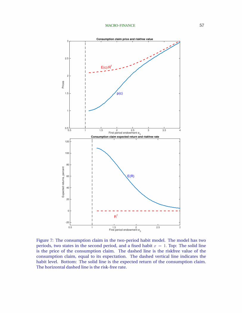
MACRO-FINANCE 57

First period endowment e0

0.5 1 1.5 2 2.5 3 3.5 4

Price

s

0.5

1

1.5

2

2.5

3

p(c)

E(c)/Rf

Consumption claim price and riskfree value

First period endowment e0

0.5 1 1.5 2 2.5 3

Exp

ecte

d r

etu

rns,

pe

rce

nt

-20

0

20

40

60

80

100

120

E(R)

Rf

Consumption claim expected return and riskfree rate

Figure 7: The consumption claim in the two-period habit model. The model has twoperiods, two states in the second period, and a fixed habit x = 1. Top: The solid lineis the price of the consumption claim. The dashed line is the riskfree value of theconsumption claim, equal to its expectation. The dashed vertical line indicates thehabit level. Bottom: The solid line is the expected return of the consumption claim.The horizontal dashed line is the risk-free rate.

MACRO-FINANCE 58

of our original habit model. Here, the linear capital accumulation technology enforces

the constant riskfree rate, and consumption is no longer a random walk.

3.2. Investment

The plot of investment with stock prices, Figure 4, and the model’s price-consumption

ratio in Figure 7 would seem to drive our desired result: Consumption “demand” falls,

investment “demand” falls, and we have a recession. It’s almost a multiplier-accelerator.

However, getting such effects in a complete model is not as easy as it sounds.

I add investment in a risky technology to the opportunity set. By investing an amount

i0 at time zero, the consumer can get a random amount θ1i0 at time 1, where θ1 ={θh, θl

}= {1.2, 0.7}. θ1 is the ex-post rate of return. In the good state and on aver-

age, with Rf = 1 or 0%, a 99% chance of a θ1 = 1.2 or 20% return is a very attractive

opportunity. However, that attraction must be balanced with a 1% risk of a -30% return,

coincident with a bad endowment shock.

The technology is now

c1 = e1 + θ1i0 +B0

c0 = e0 − i0 −B0/Rf

i0 ≥ 0; θ1 ={θh, θl

}.

Here B0 is investment in the safe Rf = 0 technology and i0 is investment in the risky

technology. I impose positive investment at time zero. Without that feature, in bad e0

times, the consumer keeps consumption c0 high, by operating the production tech-

nology in a strongly negative manner, shifting consumption from the high productivity

state to the low-productivity state. This ability is unrealistic. A real model will have ad-

justment costs, irreversibility, and depreciation, and won’t let you turn low productivity

states into high ones by a negative capital stock. Here, i0 > 0 does the same trick.

MACRO-FINANCE 59

The consumer has two investment opportunities in this model. I want to think of i0 and

θ1 as real, physical investment in productive but risky opportunities. I want to think of

B0 as riskfree storage, government bonds, or borrowing and lending abroad. The point is

to capture the effects of risk aversion in shifting the composition of investment demand,

a “flight to quality,” or a response to bad times by shaping the riskiness of the production

technology.

Maximizing the same objective

max

{(c0 − x)1−γ

1− γ+ βE

[(c1 − x)1−γ

1− γ

]}with this enhanced technology, the model solution is characterized by two first order

conditions

(c0 − x)−γ = E(c1 − x)−γ

(c0 − x)−γ = E[(c1 − x)−γθ1

]if i0 > 0.

Again, I solve numerically for c0, using the same parameters.

Figure 8 presents consumption c0, ch, cl, physical investment i0, and riskfree investment

B for this model. Figures 9 and 9 present the price and expected return of the consump-

tion claim and the new risky technology.

Starting at the right-hand side of Figure 8 and moving left, we initially see roughly per-

manent income behavior of consumption c0, falling with a slope about 1/2 in response

to losses in initial income e0.

We also see leverage, a negative investment in the riskfree technology and a large pos-

itive investment in the risky technology. As the initial endowment falls, moving left,

however, investment in the risky technology falls fast, and investment in riskfree tech-

nology rises. The consumer is worried about making sure consumption in the bad state

stays above habit. Where before he or she had to do this by reducing consumption at

MACRO-FINANCE 60

First period endowment e0

0.5 1 1.5 2 2.5 3 3.5 4

Consum

ption c

-1

-0.5

0

0.5

1

1.5

2

2.5

3

cl

c0

ch

Investment i

Storage/debt B

Consumption and Investment

Figure 8: Consumption and investment as a function of time-0 endowment. The modelhas two periods, two technologies and a fixed habit. One technology B is riskfree withreturn Rf = 1. The second technology is risky, investment i produces a rate of returnthat is either 20% with 99% probability, or -30% with 1% probability. The second-periodendowment is also risky, either equal to 2 or to 0.9 in the same good and bad states.The solid line labeled c0 gives time-0 consumption. The solid line labeled “Investmenti” gives investment in the risky technology. The dashed line labeled “Storage/debt B”gives investment in the risk-free technology. The dashed lines labeled “ch” and “cl” giveconsumption at date 1 in the good and bad states respectively. The angled solid linegives the 45 degree line c0 = e0 for reference.

time 0, saving more overall for time 1 just in case, now the consumer can instead back

away from risky investment, substituting risk-free investment, and keeping current con-

sumption high. We see a “flight to quality,” a strong fall in private investment and larger

demand for government bonds or storage. We see “deleveraging” as the large invest-

ments in the risky technology had been financed by negative positions in the riskfree.

MACRO-FINANCE 61

By changing the relative proportions invested in the two technologies, the consumer is

able to shape the riskiness of his or her overall production technologies independently

of the overall level of saving. More risk-averse consumers demand less risk overall, and

they can get it by substituting one kind of investment for another. This phenomenon is

overlooked by standard macroeconomic models that posit a single production technol-

ogy, and give consumers no control over the riskiness of that technology.

Moving to the left some more, once investment in the risky technology hits the con-

straint i0 ≥ 0, the option to insure the bad time-1 state by reducing risky investment

is exhausted. Now the consumer must severely cut back on time zero consumption,

leaving unconditional time 1 resources to cover the bad state. Here we see the high

marginal propensity to consume behavior again. As before however, this propensity is

not motivated by intertemporal substitution of consumption today for expected con-

sumption in the future; it is worst-case, “rare disaster” “ambiguity averse” behavior,

accepting too much future consumption in 99% of the states, but keeping just enough

around to stay alive in the worst-possible state.

Thus, we have the second part of the multiplier / accelerator story. As initial wealth de-

creases, equilibrium physical investment collapses, along with “deleveraging,” reducing

the debt used to finance that investment. As wealth decreases even more, investment

collapses to zero and all savings go in to the riskless opportunity.

The asset pricing figure 9 shows the same difference in behavior in the constrained

and unconstrained regions. In the constrained region, the price of the consumption

clam and technology fall sharply, as their expected returns rise. In the unconstrained

region, the price of the technology is one, as this model has no adjustment costs, and

its expected return is constant. Running in to the constraint at which one would like to

reverse risky investments thus leads to precipitous price drops. All of these phenomena

have obvious suggestive analogies to the 2008-2016 experience.

MACRO-FINANCE 62

First period endowment e0

0.5 1 1.5 2 2.5 3 3.5 4

Price

s

0

0.5

1

1.5

2

2.5

3

p(c)

p(θ)

E(c)/Rf

Asset Prices

First period endowment e0

0.5 1 1.5 2 2.5 3

Exp

ecte

d r

etu

rns,

pe

rce

nt

-20

0

20

40

60

80

100

120

E(R) cons. claim

E(R) production

E(R) cons. claim

Rf

Expected return and riskfree rate

Figure 9: Price and expected return of consumption claim and investment technologyin the two-technology two-date habit model. Top: The solid line labeled p(c) gives theprice of a consumption claim. The solid line labeled p(θ) gives the price of the riskytechnology {θh, θl}. The dashed line labeled “E(c)/Rf” gives the riskfree expected valueof the consumption claim. Bottom: The solid line marked “E(R) cons. claim” is theexpected return of the consumption claim. The solid line marked “E(R) production” isthe expected return of the risky technology, {θh, θl}. The dashed line marked “Rf” is theriskfree rate.

MACRO-FINANCE 63

3.3. On to recessions (someday)

We have the two main ingredients of a theory of risk-averse recessions – consumption

falls, with marginal propensities approaching one, and investment in risky private tech-

nologies falls dramatically, along with leverage used to finance investment.

However, turning such “demand” into actual recessions requires additional steps, as

always in macroeconomics. “Demand” may fall, but if Y = F (K,L), and capital and

labor have not changed, why should output fall? Put another way, if the marginal utility

of consumption rises so much, why does the consumer not work harder to finance that

consumption?

To illustrate the point in a simple static model, include labor hours n, less than total

available hours h, and include leisure h−n in the utility function. Also add the opportu-

nity to produce the consumption good c = wn. Then, the consumer’s objective is

max{

(c− x)1−γ + (h− n)1−γ}

s.t. c = wn

and the first order condition is

(c− x) = w(h− n).

So, in a state that consumption cwould otherwise fall close to habit x, the consumer will

instead work more n, until labor hours rise towards the maximum available h. Of course,

we do not see this – hours fall in recessions, they don’t rise.

At a minimum, this example suggests that successfully incorporating leisure and other

goods into the habit utility function will require habits of their own. And that is not

unreasonable. Our ancestors worked 12 hours a day or more. Rearranging lives, legal

limitations, and the fraction of a household that works, to accommodate much greater

work hours might take time. The effective maximum number of hours may indeed

MACRO-FINANCE 64

evolve like a habit. But even that modification will not address the cyclical fall of em-

ployment.

Similarly, the central puzzle of macroeconomics is dissonance between saving and in-

vestment. If consumers want to save more, why does investment fall?

The usual response to these two puzzles is to add frictions, such as sticky prices and

wages, financial frictions or investment irrationalities, and monopolistic competition,

such that output and labor effort follow consumption and investment “demand,” not

labor supply or the supply of savings. One may end up following that traditional route.

However, it strikes me that in this context, risk-averse recessions may emerge even with-

out relying on nominal stickiness, as follows.

First, let us think about riskless investment B as storage, government debt, or inter-

national borrowing and lending. The interpretation as government debt I think is the

clearest, as the 2008 recession featured a “flight to quality” surge in the demand for

government debt along with a collapse in demand for private securities and invest-

ment.

Then the dramatic portfolio shift in investment from the consumer’s point of view,

from risky technology to risk-free government debt, is a dramatic reduction in actual

investment in private capital stock. This shift answers the classic puzzle how a larger

desire to save, especially via precautionary savings, does not translate into larger private

investment – with no real or financial frictions required.

However, labeling the riskfree opportunity as government debt requires some slight of

hand. The model states that the government really can transfer real resources through

time. In reality government debt is a claim on future taxes. Only if the larger supply

of government debt really is “invested,” as our politicians love to call spending, in in-

frastructure or other projects that actually lead to larger future output and tax revenue,

can we use the equations of this model with that label. Lending abroad can work for

an individual economy, as real resources come back, but at a global level the riskfree

MACRO-FINANCE 65

debt must actually correspond to riskfree opportunities, or the perception (Ricardian

failures) of such opportunities.

Second, let us regard all private production as, to some extent, investment in a risky

project. When a worker shows up at a car factory, steel factory, or even a bank, he

or she is not producing a consumption good that can be consumed immediately. He

or she is participating in a risky investment project. In reality, there really is nothing

a typical worker can do, if the risky firm he or she is working at in Fall of 2008 shuts

down, to produce anything of immediate consumption value. The production equation

c = wn does not represent an actual technological opportunity. It even takes time

to sign up to drive for Uber. The storied stockbrokers selling apples may not show a

failure of the employment market, but the paucity of production opportunities to create

consumption goods today.

As a set of equations that captures these ideas, let us write the model now as

max{

(c0 − x)1−γ + E(c1 − x)1−γ} s.t.

c1 = e1 + θ1 min (i0, n0) +B0

c0 = e0 − i0 −B0

i0 ≥ 0;h > n0 > 0

In this formulation, labor n0 is complementary with investment i0, and both produce

consumption goods tomorrow at time 1, not immediately. As a result, labor falls exactly

with investment i0 = n0.

By specifying an inelastic labor supply, the solution of this model is exactly the same as

the last model, so I don’t have to solve any more equations. Now the fall in investment

i0 is the fall in labor n0 and a fall in output.

Thus, by identifying the private economy as entirely and unavoidably devoted to the

MACRO-FINANCE 66

risky production technology, we have private output decline, private investment de-

cline, and private labor decline in bad times, without the need for any stickiness.

The central mechanism is that which conventional macroeconomics rules out: because

risk aversion increases, people want to reallocate investment, both of their resources and

their labor effort (if they could) from risky to riskfree technologies. Private technologies

are inherently risky, so we see the huge demand for government debt, and the collapse

of private output, investment, and labor.

Of course this is only a suggestive and stylized two-period model. The point, for an essay

such as this: The big lesson of finance is that risk premiums vary over time, coordinated

across asset classes, and correlated with recessions. The lesson of finance for macroe-

conomics then ought to be, that risk premiums and risk aversion, not riskfree rates and

intertemporal substitution, are the central features of recessions. The fall in investment

coincident with a rise in savings at the center of Keynesian economics can result from

the fact that people want to reallocate investment to less risky projects even more than

they want to save and invest more overall.

But all that awaits a real, complete, dynamic model.

4. Summary

In summary, we have learned that asset prices correspond to a large, time-varying, business-

cycle correlated risk premium. This risk premium means that price ratios forecast re-

turns, and thus that the risk premium accounts entirely for the high volatility of price

ratios.

A representative consumer model with habit preferences captures this phenomenon. It

does so parsimoniously, in that the variation in risk premium is endogenous, and with

a specific and rejectable independent measurement of its state variable, the relation of

MACRO-FINANCE 67

consumption to its recent past.

Lots of other modeling approaches capture the same facts, with a wide range of al-

ternative underlying ideas and intuitions, including long-run risk, idiosyncratic risk,

wealth shifts among agents with heterogenous preferences, debts and balance sheets,

psychological or ambiguity-averse probability distortions, and time-varying rare disas-

ter probabilities. Many of these models embody the same intuitions. I have emphasized

that habit models behave much like rare-disaster, probability-distorted, or ambiguity

averse models that focus on bad states; the converse interpretations work as well.

None of these modeling approaches stands above the others in the list of facts so far

addressed. A serious effort to distinguish them has not been made. But, given the

fact that the state variables are so correlated, and that the models are all quantitative

parables not detailed models-of-everything meant to be literally true, that effort may

not be worth the bother. They differ, as I have pointed out, somewhat in the ratio of

assumptions to predictions, and the amount of “dark matter” invoked to explain various

phenomena, and more deeply they differ in the analytical convenience they each have in

capturing the common ideas. The latter may be the most important feature for modeling

developments.

As I look to the future, it seems time for this body of empirical and theoretical knowledge

to invade macroeconomics. Recessions are phenomena of risk premiums, risk aversion,

risk bearing capacity, desires to shift the composition of a portfolio from risky to risk free

assets, a “flight to quality,” not a phenomenon of intertemporal substitution, a desire to

consume more tomorrow vs. today.

My vision applies equally if one thinks the variation in risk premium is “irrational,” or

the result of intermediary agency frictions. If one takes that view, then via the admirably

fitting (see Figure 4) Q theory, financial market movements drive business cycles, and

we’re looking in all the wrong places for the causality (real to asset price vs. asset price

to real) and nature of business cycles.

MACRO-FINANCE 68

That invasion of macroeconomics strikes me as even more interesting and productive

than what macro-finance has accomplished so far to understand asset price movements,

and most of my purpose in writing this essay has been to encourage you to join me in its

quest.

References

Bansal, Ravi, Dana Kiku, and Amir Yaron. 2012. “An Empirical Evaluation of the Long-

Run Risks Model for Asset Prices.” Critical Finance Review 1:183–221.

Bansal, Ravi, and Amir Yaron. 2004. “Risks for the Long Run: A Potential Resolution of

Asset Pricing Puzzles.” The Journal of Finance 59:1540–6261.

Barro, Robert J. 2006. “Rare Disasters and Asset Markets in the Twentieth Century.” The

Quarterly Journal of Economics 121:823–866.

Beeler, Jason, and John Y. Campbell. 2012. “The Long-Run Risks Model and Aggregate

Asset Prices: An Empirical Assessment.” Critical Finance Review 1:141–182.

Belo, Frederico. 2010. “Production-Based Measures of Risk for Asset Pricing.” Journal of

Monetary Economics 57:146–163.

Brunnermeier, Markus. 2009. “Deciphering the Liquidity and Credit Crunch 2007-08.”

Journal of Economic Perspectives 23:77–100.

Campbell, John Y., and John H. Cochrane. 1999a. “By Force of Habit: A Consumption-

Based Explanation of Aggregate Stock Market Behavior.” Journal of Political Econ-

omy 107:205–251.

. 1999b. “By Force of Habit, Manuscript with Unpublished Appendices.” http://

faculty.chicagobooth.edu/john.cochrane/research/papers/habit.pdf.

. 2000. “Explaining the Poor Performance of Consumption-Based Asset Pricing

Models.” Journal of Finance 55:2863–2878.

MACRO-FINANCE 69

Campbell, John Y., Carolin Pflueger, and Luis M. Viceira. 2015. “Monetary Policy Drivers

of Bond and Equity Risks.” http : / / scholar . harvard . edu / files / campbell / files /

campbellpfluegerviceira 20150609.pdf.

Chen, Hui, Winston Dou, and Leonid Kogan. 2015. “Measuring the ‘Dark Matter’ in Asset

Pricing Models.”

Cochrane, John H. 1988. “How Big is the Random Walk in GNP?” Journal of Political

Economy 96:893–920.

. 2004. Asset Pricing, Revised Edition. Princeton University Press.

. 2007. “Financial Markets and the Real Economy.” In Handbook of the Equity

Premium, edited by Rajnish Mehra, 237–325. Elsevier.

. 2011. “Discount Rates: American Finance Association Presidential Address.” Jour-

nal of Finance 66:1047–1108.

Cochrane, John H., and Monika Piazzesi. 2005. “Bond Risk Premia.” American Economic

Review 95:138–160.

. 2008. “Decomposing the Yield Curve.” http://faculty.chicagobooth.edu/john.

cochrane/research/papers/interest rate revised.pdf.

Constantinides, George M., and Darrell Duffie. 1996. “Asset Pricing with Heterogeneous

Consumers.” Journal of Political Economy 104:219–240.

DePaoli, Bianca, and Pawel Zabczyk. 2012. “Cyclical Risk Aversion, Precautionary Saving,

and Monetary Policy.” Journal of Money, Credit and Banking 45:1–36.

Diercks, Anthony M. 2015. “The Equity Premium, Long-Run Risk, & Optimal Monetary

Policy.” FEDS Working Paper No. 2015-087. http://ssrn.com/abstract=2670122.

Epstein, Larry G., Emmanuel Farhi, and Tomasz Strzalecki. 2014. “How Much Would You

Pay to Resolve Long-Run Risk?” American Economic Review 104:2680–2697.

MACRO-FINANCE 70

Epstein, Larry G., and Stanley E. Zin. 1989. “Substitution, Risk Aversion, and the Tempo-

ral Behavior of Consumption and Asset Returns: A Theoretical Framework.” Econo-

metrica 57:937–69.

Fama, Eugene F. 1970. “Efficient Capital Markets: A Review of Theory and Empirical

Work.” The Journal of Finance 25:383–417.

Gabaix, Xavier. 2012. “Variable Rare Disasters: An Exactly Solved Framework for Ten

Puzzles in Macro-Finance.” Quarterly Journal of Economics 127:645–700.

Garleanu, Nicolae, and Stavros Panageas. 2015. “Young, Old, Conservative, and Bold:

The Implications of Heterogeneity and Finite Lives for Asset Pricing.” Journal of

Political Economy 123:670–685.

Grishchenko, Olesya V., Zhaogang Song, and Hao Zhou. 2015. “Term Structure of Interest

Rates with Short-Run and Long-Run Risks.” http://ssrn.com/abstract=2663357.

Hansen, Lars Peter, John Heaton, and Nan Li. 2008. “Consumption Strikes Back?: Mea-

suring Long Run Risk.” Journal of Political Economy 116:260–302.

Hansen, Lars Peter, and Ravi Jagannathan. 1991. “Implications of security market data

for models of dynamic economies.” Journal of Political Economy 99:225–262.

Hansen, Lars Peter, and Thomas J. Sargent. 2001. “Robust Control and Model Uncer-

tainty.” American Economic Review 91:60–66.

Harrison, J Michael, and David M Kreps. 1979. “Martingales and arbitrage in multiperiod

securities markets.” Journal of Economic theory 20 (3): 381–408.

Harvey, Campbell R., Yan Liu, and Heqing Zhu. 2016. “... and the cross-section of ex-

pected returns.” Review of Financial Studies 29:5–68.

Jagannathan, Ravi, and Yong Wang. 2007. “Lazy Investors, Discretionary Consumption,

and the Cross-Section of Stock Returns.” The Journal of Finance 62:1623–1661.

MACRO-FINANCE 71

Jermann, Urban J. 2013. “A Production-Based Model for the Term Structure.” Journal of

Financial Economics 109:293–306.

Kandel, Shmuel, and Robert F. Stambaugh. 1990. “Expectations and volatility of con-

sumption and asset returns.” Review of Financial Studies 3:207?232.

Krishnamurthy, Arvind, and Zhiguo He. 2013. “Intermediary Asset Pricing.” American

Economic Review 103:732?770.

Leonid, Kogan, Dimitris Papanikolaou, and Noah Stoffman. 2016. “Winners and Losers:

Creative Destruction and the Stock Market.”

Lettau, Martin, and Sydney Ludvigson. 2001. “Consumption, Aggregate Wealth and Ex-

pected Stock Returns.” Journal of Finance 56:815–849.

Lettau, Martin, Syndey C. Ludvigson, and Sai Ma. 2015. “Capital Share Risk and Share-

holder Heterogeneity in U.S. Stock Pricing.” http://www.sydneyludvigson.com/s/

lbs.pdf.

Lopez, Pierlauro, David Lopez-Salido, and Francisco Vazquez-Grande. 2015. “Nominal

Rigidities and the Term Structures of Equity and Bond Returns.” http://dx.doi.org/

10.2139/ssrn.2626619.

Oster, Emily, Ira Shoulson, and E. Ray Dorsey. 2013. “Optimal Expectations and Limited

Medical Testing: Evidence from Huntington Disease.” American Economic Review

103:804–30.

Piazzesi, Monika, Martin Schneider, and Selale Tuzel. 2007. “Housing, Consumption,

and Asset Pricing.” Journal of Financial Economics 83:531–569.

Reitz, Thomas A. 1988. “The Equity Risk Premium: A Solution.” Journal of Monetary

Economics 22:117–31.

Schmidt, Lawrence. 2015. “Climbing and Falling Off the Ladder: Asset Pricing Implica-

tions of Labor Market Event Risk.”

MACRO-FINANCE 72

Shiller, Robert J. 1981. “Do stock prices move too much to be justified by subsequent

changes in dividends?” American Economic Review 71:421–436.

Shiller, Robert J. 2014. “Speculative Asset Prices.” American Economic Review 104:1486–

1517.

Tallarini, Thomas D. 2000. “Risk-Sensitive Real Business Cycles.” Journal of Monetary

Economics 45:507–532.

Tallarini, Thomas D., and Harold H. Zhang. 2005. “External Habit and the Cyclicality of

Expected Stock Returns.” Journal of Business 78:1023–1048.

Verdelhan, Adrien. 2010. “A Habit-Based Explanation of the Exchange Rate Risk Pre-

mium.” Journal of Finance 65:123–145.

Wachter, Jessica. 2006. “A consumption-based model of the term structure of interest

rates.” Journal of Financial Economics 79:365–399.

Welch, Ivo. 2016. “The (Time-Varying) Importance of Disaster Risk.” Financial Analysts

Journal 72:Forthcoming.