macro factors in oil futures returns
TRANSCRIPT

Introduction Data Factor computation Fitting oil return Conclusion
Macro Factors in Oil Futures Returns
Yannick LE PEN
PSL*, Universite de Paris-Dauphine, LEDa-CGEMP
Benoıt SEVI
Aix-Marseille Universite, CNRS & EHESS
2eme Seminaire Academique d’Economie de l’Energie
Mercredi 13 Fevrier 2013
Introduction Data Factor computation Fitting oil return Conclusion
The framework
• Which causes affect oil price in the late 2000s?
• Speculation or rising demand?
• Buyuksahin et al. (2008), Hamilton (2009), Kilian (2009),
Buyuksahin and Harris (2011), Parsons (2010), Kaufmann (2011)
and Tang and Xiong (2011) :
1. No evidence of causality from speculation to price.
2. Minor role of trading activity in the NYMEX WTI in the 2008 price
peak formation.
• Hamilton (2009): the 2008 oil price increase attributed to a
“demand shock” which may have its origin in Asia and more
particularly in China.

Introduction Data Factor computation Fitting oil return Conclusion
The framework (con’t)
• Standard analysis of macro factors for crude oil returns: Brown and
Yucel (2002) or Lescaroux and Mignon (2008) (among others).
• Kilian and Vega (2011)
• No evidence of an impact of US macroeconomic news on daily price
changes in the oil spot market.
• But:
• Macroeconomic news may impact longer maturity futures contracts
• U.S. news: a part of the story.
• We extend Kilian and Vega (2011) analysis and consider a set of
macroeconomic variables representative of developped and emerging
countries.

Introduction Data Factor computation Fitting oil return Conclusion
Two objectives of the paper
1. How useful is a large set of international real and nominal variables
in explaining crude oil return?
• We gather a set of 187 real and nominal macroeconomics variables
from developped and emerging countries.
• We apply “Large approximate factor model” ( Stock and Watson
(2002) to extract factors from these data.
• These factors represent demand related “fundamentals”.
• Avoid to select an a priori set of explanatory variables. We expect to
minimize the risk of omitted variable.
2. How can we interpret the factors that have the best explanatory
power?
• We look at the explanatory power of each factor for the original
series.
• A criterion proposed by Ludvigson and Ng (2009)

Introduction Data Factor computation Fitting oil return Conclusion
Related literature
• Zagaglia (2010): a paper related to ours.
• Applies the large factor model method.
• Uses variables related to the US economy and oil and oil derivates
times series. Criticized by Alquist et al. (2011) for doing so.
• We include in our database real and nominal variables from
developed and emerging countries.

Introduction Data Factor computation Fitting oil return Conclusion
Sketch of results
• Our “best” model explains around 38% of oil returns variability
• The factor with the highest explanatory power is mainly correlated
with real variables from emerging countries.

Introduction Data Factor computation Fitting oil return Conclusion
Outline of the presentation
Introduction
Data
Factor computation
Fitting oil return
Conclusion

Introduction Data Factor computation Fitting oil return Conclusion
Oil futures and Macroeconomic database
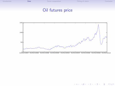
• Monthly futures prices for the NYMEX WTI
• Time period: 1993:11 to 2010:03 (197 monthly observations).
• We use monthly observations to match with macroeconomic
variables frequency.
Introduction Data Factor computation Fitting oil return Conclusion
Oil futures price
01/01/1994 01/01/1996 01/01/1998 01/01/2000 01/01/2002 01/01/2004 01/01/2006 01/01/2008 01/01/20100
50
100
150

Introduction Data Factor computation Fitting oil return Conclusion
Oil futures return
01/01/1994 01/01/1996 01/01/1998 01/01/2000 01/01/2002 01/01/2004 01/01/2006 01/01/2008 01/01/2010
−0.4
−0.3
−0.2
−0.1
0
0.1
0.2
0.3
Return is computed as the price log difference
Introduction Data Factor computation Fitting oil return Conclusion
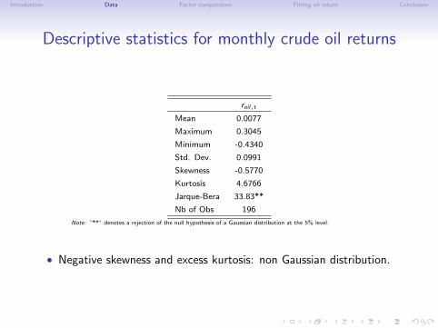
Descriptive statistics for monthly crude oil returns
roil,t
Mean 0.0077
Maximum 0.3045
Minimum -0.4340
Std. Dev. 0.0991
Skewness -0.5770
Kurtosis 4.6766
Jarque-Bera 33.83**
Nb of Obs 196
Note: “**” denotes a rejection of the null hypothesis of a Gaussian distribution at the 5% level.
• Negative skewness and excess kurtosis: non Gaussian distribution.

Introduction Data Factor computation Fitting oil return Conclusion
Macroeconomic database
• 187 international macroeconomic and nominal variables
representative of the world economy
• 128 variables for Developed economies and 59 variables for emerging
countries.
• 103 real variables (73 for developed countries, 30 for emerging
countries) and 84 nominal variables (55 for developed and 29 for
emerging countries).
• Differ from Stock and Watson (2005) and Ludvigson and Ng (2009)
mainly focused on the US economy.
• Before computation, data are stationarized using the appropriate
transformation if needed (first difference, log first difference,...).
• All data extracted from DataStream.

Introduction Data Factor computation Fitting oil return Conclusion
Large approximate factor model
• Let xi,t = observation of the i th time series (i = 1, ...,N) at date t
(t = 1, ...,T )
• Selecting relevant variables among N variables when N is large is not
possible ; we then resort to a set of r factors:
xit = λ′
iFt + eit
• Ft : vector of the r common factors.
• eit : idiosyncratic error
• λi : factor loadings of the (static) common factors
• Computation of factors via principal component analysis.
Introduction Data Factor computation Fitting oil return Conclusion
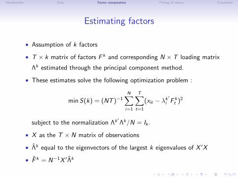
Estimating factors
• Assumption of k factors
• T × k matrix of factors F k and corresponding N × T loading matrix
Λk estimated through the principal component method.
• These estimates solve the following optimization problem :
minS(k) = (NT )−1N∑i=1
T∑t=1
(xit − λk′
i F kt )2
subject to the normalization Λk′Λk/N = Ik .
• X as the T × N matrix of observations
• Λk equal to the eigenvectors of the largest k eigenvalues of X ′X
• F k = N−1X ′Λk

Introduction Data Factor computation Fitting oil return Conclusion
Selecting the number of factors
• Bai and Ng (2002) information criteria: an extension to factor
model of usual information criteria (AIC..).
PCPi (k) = S(k) + kσ2gi (N,T )
ICi (k) = ln(S(k)) + kgi (N,T )
• S(k) residual sum of square, gi penalty function, σ2 = S(kmax) for a
pre-specified value kmax
• Kapetanios (2009) sequential test for determining the number of
factors
Introduction Data Factor computation Fitting oil return Conclusion
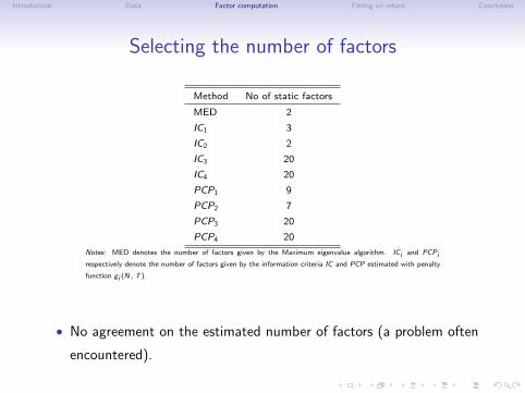
Selecting the number of factors
Method No of static factors
MED 2
IC1 3
IC2 2
IC3 20
IC4 20
PCP1 9
PCP2 7
PCP3 20
PCP4 20
Notes: MED denotes the number of factors given by the Maximum eigenvalue algorithm. ICi and PCPi
respectively denote the number of factors given by the information criteria IC and PCP estimated with penalty
function gi (N, T ).
• No agreement on the estimated number of factors (a problem often
encountered).

Introduction Data Factor computation Fitting oil return Conclusion
Selecting the number of factors: summary statistics
Ft,i i ρ1 ρ2 ρ3 R2i
1 0.1614 0.1256 0.3176 0.0975
2 0.1357 0.0805 0.3110 0.1619
3 -0.0748 0.0145 -0.0294 0.2030
4 -0.0765 -0.0910 0.1508 0.2355
5 -0.2180 -0.0763 0.1213 0.2654
6 0.1801 0.0388 0.0267 0.2927
7 0.0721 0.2765 0.2744 0.3185
8 0.4086 0.5013 0.3332 0.3418
9 -0.0066 -0.0305 -0.0379 0.3636
Note: ρi denotes the i th autocorrelation. R2i : fraction of total variance
in the data explained by factors 1 to i.
• We select the first 9 factors which explain 36 % of the total variance
in the data.
Introduction Data Factor computation Fitting oil return Conclusion
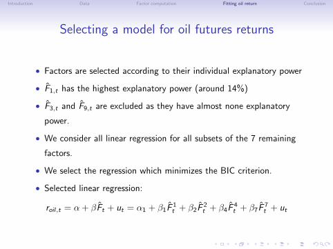
Selecting a model for oil futures returns
• Factors are selected according to their individual explanatory power
• F1,t has the highest explanatory power (around 14%)
• F3,t and F9,t are excluded as they have almost none explanatory
power.
• We consider all linear regression for all subsets of the 7 remaining
factors.
• We select the regression which minimizes the BIC criterion.
• Selected linear regression:
roil,t = α + βFt + ut = α1 + β1F1t + β2F
2t + β4F
4t + β7F
7t + ut
Introduction Data Factor computation Fitting oil return Conclusion
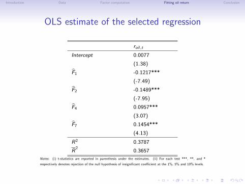
OLS estimate of the selected regression
roil,t
Intercept 0.0077
(1.38)
F1 -0.1217***
(-7.49)
F2 -0.1489***
(-7.95)
F4 0.0957***
(3.07)
F7 0.1454***
(4.13)
R2 0.3787
R2
0.3657
Notes: (i) t-statistics are reported in parenthesis under the estimates. (ii) For each test ***, **, and *
respectively denotes rejection of the null hypothesis of insignificant coefficient at the 1%, 5% and 10% levels.

Introduction Data Factor computation Fitting oil return Conclusion
Interpreting factors
• Ludvigson and Ng (2009) suggest a simple method to interpret the
estimated factors.
• Each original variable is regressed on a single factor to measure the
correlation between the former and the latter.
• The R2 are reported on a graph with a given order.
• The factor is considered as representative of the variables with
highest R2.
• Our 187 series classified into four categories according to the
characteristics real variable/nominal variable and developed
countries/emerging countries.

Introduction Data Factor computation Fitting oil return Conclusion
Interpreting factor F1
20 40 60 80 100 120 140 160 1800
0.05
0.1
0.15
0.2
0.25
0.3
0.35
0.4
0.45
0.5R
−squ
are
Marginal R−squares for F1
real, dev
nominal, dev
real, emerging
nominal,emerging
• F 1t interpreted as a real factor.
• Mostly correlated with real variables from emerging countries
• An evidence of the growing weight of emerging countries in shaping
oil price.
Introduction Data Factor computation Fitting oil return Conclusion
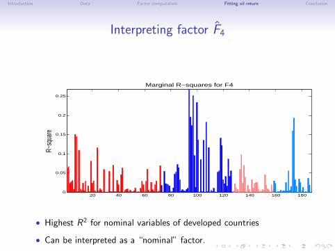
Interpreting factor F4
20 40 60 80 100 120 140 160 1800
0.05
0.1
0.15
0.2
0.25
R−sq
uare
Marginal R−squares for F4
• Highest R2 for nominal variables of developed countries
• Can be interpreted as a “nominal” factor.

Introduction Data Factor computation Fitting oil return Conclusion
Interpreting factor F2
20 40 60 80 100 120 140 160 1800
0.05
0.1
0.15
0.2
0.25
0.3
0.35
0.4
0.45
R−s
quar
e
Marginal R−squares for F2
• More difficult to interpret
• Highest R2 with a subset of agregate consumption of developed
countries

Introduction Data Factor computation Fitting oil return Conclusion
Interpreting factor F7
20 40 60 80 100 120 140 160 1800
0.05
0.1
0.15
0.2
R−sq
uare
Marginal R−squares for F7
Also correlated with real variables of developed countries

Introduction Data Factor computation Fitting oil return Conclusion
Limits and extensions
1. Enlarging the database
• Data on inventories and production
• Checking the relevance of the series in the database (Boivin and Ng
(2006))
2. More sophisticated econometric methods
• Comparison with dynamic factor models (more appropriate for a
forecasting exercise)
• Bootstrapping factors (Ludvigson and Ng (2009, 2010) and
Gospodinov and Ng (2010)) because factors are estimated quantities.
• Using times series of different frequencies (MIDAS).

Introduction Data Factor computation Fitting oil return Conclusion
Limits and extensions
3. The role of speculation
• Bunn, Chevallier, Le Pen and Sevi (2013) “Fundamental and
Financial Influences on the Comovement of Oil and Gas price”,
• Le Pen and Sevi (2013) “Futures trading and the excess
comovement of commodity prices”.
• We show that the commodity returns correlation is highly related to:
• the Han (2008) index of speculative activity,
• the De Roon et al. (2000) index of hedging pressure,
on commodity markets.
• We conclude that trading activity on these markets has an impact on
intercommodity correlation.