machine translation part ii 6.891: lecture 11 (october

6.891: Lecture 11 (October 15th, 2003)

Machine Translation Part II

Overview� The Structure of IBM Models 1 and 2

� EM Training of Models 1 and 2

� Some examples of training Models 1 and 2

� IBM Model 3

Recap: IBM Model 1� Aim is to model the distribution

P (f j e)

wheree is an English sentencee1 : : : el

wheref is a French sentencef1 : : : fm

� Only parameters in Model 1 aretranslation parameters:

T(f j e)

wheref is a French word,e is an English word

� e.g.,

T(le j the) = 0:7

T(la j the) = 0:2

T(l0 j the) = 0:1

Recap: Alignments in IBM Model 1� Aim is to model the distribution

P (f j e)

wheree is an English sentencee1 : : : el

wheref is a French sentencef1 : : : fm

� An alignment a identifies which English word each French wordoriginated from

� Formally, analignment a is fa1; : : : amg, where eachaj 2 f0 : : : lg.

� There are(l + 1)m possible alignments.In IBM model 1 all alignmentsa are equally likely:

P (a j e) = C �

1

(l + 1)mwhereC = prob(length(f) = m) is a constant.

IBM Model 1: The Generative Process

To generate a French stringf from an English string e:� Step 1: Pick the length off (all lengths equally probable,

probabilityC)

� Step 2: Pick an alignmenta with probability 1

(l+1)m

� Step 3: Pick the French words with probabilityP (f j a; e) =

mYj=1T(fj j eaj )

The final result:

P (f ; a j e) = P (a j e)P (f j a; e) =

C

(l + 1)mmY

j=1T(fj j eaj )

IBM Model 2� Only difference: we now introducealignment or distortion parameters

D(i j j; l;m) = Probability thatj’th French word is connected

to i’th English word, given sentence lengths of

e andf arel andm respectively

� Define

P (a = fa1; : : : amg j e; l;m) =

mYj=1D(aj j j; l;m)

� Gives

P (f ; a j e; l;m) =

mYj=1D(aj j j; l;m)T(fj j eaj )

� Note: Model 1 is a special case of Model 2, whereD(i j j; l;m) = 1l+1

for all i; j.

An Example

l = 6

m = 7

e = And the program has been implementedf = Le programme a ete mis en application

a = f2; 3; 4; 5; 6; 6; 6g

P (a j e; l = 6;m = 7) = D(i = 2 j j = 1; l = 6;m = 7)�

D(i = 3 j j = 2; l = 6;m = 7)�

D(i = 4 j j = 3; l = 6;m = 7)�

D(i = 5 j j = 4; l = 6;m = 7)�

D(i = 6 j j = 5; l = 6;m = 7)�

D(i = 6 j j = 6; l = 6;m = 7)�

D(i = 6 j j = 7; l = 6;m = 7)

P(fja;e)

=

T(Lejthe)�

T(programmejprogram)�

T(ajhas)�

T(etejbeen)�

T(misjimplemented)�

T(enjimplemented)�

T(applicationjimplemented)

IBM Model 2: The Generative Process

To generate a French stringf from an English string e:� Step 1: Pick the length off (all lengths equally probable, probabilityC)

� Step 2: Pick an alignmenta = fa1; a2 : : : amg with probability

mYj=1D(aj j j; l;m)

� Step 3: Pick the French words with probability

P (f j a; e) =

mYj=1T(fj j eaj )

The final result:

P (f ; a j e) = P (a j e)P (f j a; e) = C





� IBM Model 3

A Hidden Variable Problem� We have:

P (f ; a j e) = C


� And:

P (f j e) =X

a2A

C


whereA is the set of all possible alignments.

A Hidden Variable Problem� Training data is a set of(fk; ek) pairs, likelihood isX

k

logP (fk j ek) =X

k

logX

a2A

P (a j ek)P (fk j a; ek)

whereA is the set of all possible alignments.

� We need to maximize this function w.r.t. the translationparameters, and the alignment probabilities

� EM can be used for this problem: initialize parametersrandomly, and at each iteration choose

�t = argmax�X

i

Xa2A

P (a j ek; fk;�t�1) logP (fk; a j ek;�)

where�t are the parameter values at thet’th iteration.

Models 1 and 2 Have a Simple Structure� We havef = ff1 : : : fmg, a = fa1 : : : amg, and

P (f ; a j e; l;m) =

mYj=1P (aj; fj j e; l;m)

where

P (aj; fj j e; l;m) = D(aj j j; l;m)T(fj j eaj )

� We can think of the m (fj; aj) pairs as being generatedindependently

A Crucial Step in the EM Algorithm� Say we have the following(e; f) pair:

e = And the program has been implementedf = Le programme a ete mis en application

� Given thatf was generated according to Model 2, what is theprobability thata1 = 2? Formally:

Prob(a1 = 2 j f ; e) =

Xa:a1=2P (a j f ; e; l;m)

The Answer

Prob(a1 = 2 j f ; e) =

Xa:a1=2

P (a j f ; e; l;m)

=

D(a1 = 2 j j = 1; l = 6;m = 7)T(le j the)Pli=0D(a1 = i j j = 1; l = 6;m = 7)T(le j ei)

Follows directly because the(aj ; fj) pairs are independent:

P (a1 = 2 j f ; e; l;m) =

P (a1 = 2; f1 = Le j f2 : : : fm; e; l;m)

P (f1 = Le j f2 : : : fm; e; l;m)

(1)=

P (a1 = 2; f1 = Le j e; l;m)

P (f1 = Le j e; l;m)

(2)

=

P (a1 = 2; f1 = Le j e; l;m)Pi P (a1 = i; f1 = Le j e; l;m)

where (2) follows from (1) becauseP (f ; a j e; l;m) =Qm

j=1 P (aj ; fj j e; l;m)

A General Result

Prob(aj = i j f ; e) =

Xa:aj=i

P (a j f ; e; l;m)

=

D(aj = i j j; l;m)T(fj j ei)Pli0=0D(aj = i0 j j; l;m)T(fj j ei0)

Alignment Probabilities have a Simple Solution!� e.g., Say we havel = 6, m = 7,

e = And the program has been implemented

f = Le programme a ete mis en application

� Probability of “mis” being connected to “the”:

P (a5 = 2 j f ; e) =D(a5 = 2 j j = 5; l = 6;m = 7)T(mis j the)

Z

where

Z = D(a5 = 0 j j = 5; l = 6;m = 7)T(mis j NULL)

+ D(a5 = 1 j j = 5; l = 6;m = 7)T(mis j And)

+ D(a5 = 2 j j = 5; l = 6;m = 7)T(mis j the)

+ D(a5 = 3 j j = 5; l = 6;m = 7)T(mis j program)

+ : : :

The EM Algorithm for Model 2� Define

e[k] for k = 1 : : : n is thek’th English sentencef [k] for k = 1 : : : n is thek’th French sentence

l[k] is the length ofe[k]

m[k] is the length off [k]

e[k; i] is thei’th word in e[k]

f [k; j] is thej’th word in f [k]

� Current parameters�t�1 are

T(f j e) for all f 2 F ; e 2 E

D(i j j; l;m)

� We’ll see how the EM algorithm re-estimates theT andD

parameters

Step 1: Calculate the Alignment Probabilities� Calculate an array of alignment probabilities

(for (k = 1 : : : n), (j = 1 : : : m[k]), (i = 0 : : : l[k])):a[i; j; k] = P (aj = i j e[k]; f [k];�t�1)

=


whereei = e[k; i], fj = f [k; j], andl = l[k];m = m[k]

i.e., the probability off [k; j] being aligned toe[k; i].

Step 2: Calculating the Expected Counts� Calculate the translation counts

tcount(e; f ) =

Xi;j;k:

e[k;i]=e;

f [k;j]=fa[i; j; k]

� tcount(e; f) is expected number of times thate is aligned with

f in the corpus

Step 2: Calculating the Expected Counts� Calculate the source counts

scount(e) =

Xi;k:

e[k;i]=em[k]X

j=1a[i; j; k]

� scount(e) is expected number of times thate is aligned withany French word in the corpus

Step 2: Calculating the Expected Counts� Calculate the alignment counts

acount(i; j; l;m) =

Xk:

l[k]=l;m[k]=ma[i; j; k]

acount(j; l;m) = jfk : l[k] = l;m[k] = mgj

� Here,acount(i; j; l;m) is expected number of times thatei isaligned tofj in English/French sentences of lengthsl andm

respectively

� acount(j; l;m) is number of times that we have sentencese

andf of lengthsl andm respectively

Step 3: Re-estimating the Parameters� New translation probabilities are then defined as

P (f j e) =tcount(e; f)

scount(e)

� New alignment probabilities are defined as

P (aj = i j j; l;m) =acount(i; j; l;m)

acount(j; l;m)

This defines the mapping from�t�1 to �t

A Summary of the EM Procedure� Start with parameters�t�1 as


D(i j j; l;m)

� Calculatealignment probabilities under current parameters

a[i; j; k] =


� Calculateexpected countstcount(e; f), scount(e), acount(i; j; l;m),andacount(j; l;m) from the alignment probabilities

� Re-estimateT(f j e) andD(i j j; l;m) from the expected counts

The Special Case of Model 1� Start with parameters�t�1 as


(no alignment parameters)

� Calculatealignment probabilities under current parametersa[i; j; k] =

T(fj j ei)Pli0=0T(fj j ei0)

(becauseD(aj = i j j; l;m) = 1=(l + 1)m for all i; j; l;m).

� Calculateexpected countstcount(e; f), scount(e),

� Re-estimateT(f j e) from the expected counts




� IBM Model 3

An Example of Training Models 1 and 2

Example will use following translations:

e[1] = the dogf[1] = le chien

e[2] = the catf[2] = le chat

e[3] = the busf[3] = l’ autobus

NB: I won’t use a NULL word e0

Initial (random) parameters:

e f T(f j e)

the le 0.23the chien 0.2the chat 0.11the l’ 0.25the autobus 0.21dog le 0.2dog chien 0.16dog chat 0.33dog l’ 0.12dog autobus 0.18cat le 0.26cat chien 0.28cat chat 0.19cat l’ 0.24cat autobus 0.03bus le 0.22bus chien 0.05bus chat 0.26bus l’ 0.19bus autobus 0.27

Alignment probabilities:

i j k a(i,j,k)1 1 0 0.5264232379597262 1 0 0.4735767620402741 2 0 0.5525179956058172 2 0 0.447482004394183

1 1 1 0.4665326020665332 1 1 0.5334673979334671 2 1 0.3563645444225072 2 1 0.643635455577493

1 1 2 0.5719504383362472 1 2 0.4280495616637531 2 2 0.4390813117245082 2 2 0.560918688275492

Expected counts:

e f tcount(e; f)

the le 0.99295584002626the chien 0.552517995605817the chat 0.356364544422507the l’ 0.571950438336247the autobus 0.439081311724508dog le 0.473576762040274dog chien 0.447482004394183dog chat 0dog l’ 0dog autobus 0cat le 0.533467397933467cat chien 0cat chat 0.643635455577493cat l’ 0cat autobus 0bus le 0bus chien 0bus chat 0bus l’ 0.428049561663753bus autobus 0.560918688275492

Old and new parameters:

e f old newthe le 0.23 0.34the chien 0.2 0.19the chat 0.11 0.12the l’ 0.25 0.2the autobus 0.21 0.15dog le 0.2 0.51dog chien 0.16 0.49dog chat 0.33 0dog l’ 0.12 0dog autobus 0.18 0cat le 0.26 0.45cat chien 0.28 0cat chat 0.19 0.55cat l’ 0.24 0cat autobus 0.03 0bus le 0.22 0bus chien 0.05 0bus chat 0.26 0bus l’ 0.19 0.43bus autobus 0.27 0.57

e fthe le 0.23 0.34 0.46 0.56 0.64 0.71the chien 0.2 0.19 0.15 0.12 0.09 0.06the chat 0.11 0.12 0.1 0.08 0.06 0.04the l’ 0.25 0.2 0.17 0.15 0.13 0.11the autobus 0.21 0.15 0.12 0.1 0.08 0.07dog le 0.2 0.51 0.46 0.39 0.33 0.28dog chien 0.16 0.49 0.54 0.61 0.67 0.72dog chat 0.33 0 0 0 0 0dog l’ 0.12 0 0 0 0 0dog autobus 0.18 0 0 0 0 0cat le 0.26 0.45 0.41 0.36 0.3 0.26cat chien 0.28 0 0 0 0 0cat chat 0.19 0.55 0.59 0.64 0.7 0.74cat l’ 0.24 0 0 0 0 0cat autobus 0.03 0 0 0 0 0bus le 0.22 0 0 0 0 0bus chien 0.05 0 0 0 0 0bus chat 0.26 0 0 0 0 0bus l’ 0.19 0.43 0.47 0.47 0.47 0.48bus autobus 0.27 0.57 0.53 0.53 0.53 0.52

After 20 iterations:

e f

the le 0.94the chien 0the chat 0the l’ 0.03the autobus 0.02dog le 0.06dog chien 0.94dog chat 0dog l’ 0dog autobus 0cat le 0.06cat chien 0cat chat 0.94cat l’ 0cat autobus 0bus le 0bus chien 0bus chat 0bus l’ 0.49bus autobus 0.51

Model 2 has several local maxima – good one:

e f T(f j e)

the le 0.67the chien 0the chat 0the l’ 0.33the autobus 0dog le 0dog chien 1dog chat 0dog l’ 0dog autobus 0cat le 0cat chien 0cat chat 1cat l’ 0cat autobus 0bus le 0bus chien 0bus chat 0bus l’ 0bus autobus 1

Model 2 has several local maxima –bad one:

e f T(f j e)

the le 0the chien 0.4the chat 0.3the l’ 0the autobus 0.3dog le 0.5dog chien 0.5dog chat 0dog l’ 0dog autobus 0cat le 0.5cat chien 0cat chat 0.5cat l’ 0cat autobus 0bus le 0bus chien 0bus chat 0bus l’ 0.5bus autobus 0.5

another bad one:

e f T(f j e)

the le 0the chien 0.33the chat 0.33the l’ 0the autobus 0.33dog le 1dog chien 0dog chat 0dog l’ 0dog autobus 0cat le 1cat chien 0cat chat 0cat l’ 0cat autobus 0bus le 0bus chien 0bus chat 0bus l’ 1bus autobus 0

� Alignment parameters for good solution:

T(i = 1 j j = 1; l = 2;m = 2) = 1

T(i = 2 j j = 1; l = 2;m = 2) = 0

T(i = 1 j j = 2; l = 2;m = 2) = 0

T(i = 2 j j = 2; l = 2;m = 2) = 1

log probability= �1:91

� Alignment parameters for first bad solution:

T(i = 1 j j = 1; l = 2;m = 2) = 0

T(i = 2 j j = 1; l = 2;m = 2) = 1

T(i = 1 j j = 2; l = 2;m = 2) = 0

T(i = 2 j j = 2; l = 2;m = 2) = 1


� Alignment parameters for second bad solution:

T(i = 1 j j = 1; l = 2;m = 2) = 0

T(i = 2 j j = 1; l = 2;m = 2) = 1

T(i = 1 j j = 2; l = 2;m = 2) = 1

T(i = 2 j j = 2; l = 2;m = 2) = 0


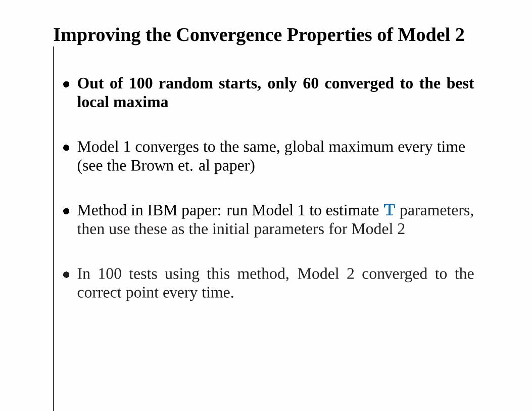
Improving the Convergence Properties of Model 2� Out of 100 random starts, only 60 converged to the best

local maxima

� Model 1 converges to the same, global maximum every time(see the Brown et. al paper)

� Method in IBM paper: run Model 1 to estimateT parameters,then use these as the initial parameters for Model 2

� In 100 tests using this method, Model 2 converged to thecorrect point every time.




� IBM Model 3

IBM Model 3� The plot thickens...

� A new type of parameter:fertility parameters

� A quite different structure to the model...

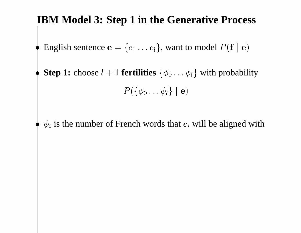
IBM Model 3: Step 1 in the Generative Process� English sentencee = fe1 : : : elg, want to modelP (f j e)

� Step 1: choosel + 1 fertilities f�0 : : : �lg with probability

P (f�0 : : : �lg j e)

� �i is the number of French words thatei will be aligned with

IBM Model 3: Fertility Parameters� New type of parameter

F(� j e) = probability thate is aligned with� words

� For example

F(0 j the) = 0:1

F(1 j the) = 0:9

F(2 j the) = 0

: : :

F(0 j not) = 0:01

F(1 j not) = 0:09

F(2 j not) = 0:9

: : :

IBM Model 3: Fertility Parameters� Step 1: choosel + 1 fertilities f�0 : : : �lg with probability

P (f�0 : : : �lg j e) = P (�0 j �1 : : : �l)lY

i=1F(�i j ei)

IBM Model 3: Fertility Parameters� ModelingP (�0 j �1 : : : �l)

� Take a single parameterp1 2 [0 : : : 1]. DefineP (�0 j �1 : : : �l) =

m!

(m� �0)!�0!p�0

1 (1� p1)m��0

wherem =Pl

i=1 �i

� Probability of seeing�0 heads if you toss a coin withprobabilityp1 of headsm times

� Intuition: m =

Pli=1 �i words have been generated from

“real” English words; for each of thesem words we generatean additional word connected toNULL with probabilityp1

IBM Model 3: The Final Fertility Model� Step 1: choosel + 1 fertilities f�0 : : : �lg with probability

P (f�0 : : : �lg j e) =

m!

(m� �0)!�0!p�0

1 (1�p1)m��0

lYi=1F(�i j ei)

� Parameters of the model are

p1and

F(� j e) for � = f0; 1; 2; : : :g, e 2 E

IBM Model 3: The Distortion and Translation Parameters� Step 2: For eachei, for k = 1 : : : �i, choose a position�i;k 2

1 : : : m and a French wordfi;k with probability

lYi=0

�iYk=1R(�i;k j i; l;m)T(fi;k j ei)

� Note that we now havereverse distortion parameters

R(j j i; l;m) = probability of French positionj given it’s

generated from English positioni

� Before we haddistortion parameters

D(i j j; l;m) = probability of English positioni given it’s

generating French positionj

IBM Model 3: Final Model

� = f�0 : : : �mg

� = f�i;k : i = 0 : : : m; k = 1 : : : �ig

f2 = ffi;k : i = 0 : : : m; k = 1 : : : �ig

P (�; �; f2 j e) =

m!

(m� �0)!�0!p�01 (1�p1)m��0

lYi=1F(�i j ei)

! lY

i=0


!

IBM Model 3: Alignments� Note that givenff2; �; �g, we can recover an alignmenta

� For a given alignmenta, we can calculatem, and�, and thereare

lYi=0�i!

ff2; �g pairs which could produce the alignment from�.

P (f ; a j e) =

m!

(m� �0)!�0!p�01 (1�p1)m��0�0!

lYi=1F(�i j ei)�i!

! lY

i=0


!

wherem;�; �; f2 are direct functions ofa

A final simplification:R(�0;k j i; l;m) is chosen so as to cancel the�0! term:

P (f ; a j e) =

m!

(m� �0)!�0!p�0

1

(1�p1)m��0

lYi=1F(�i j ei)�i!

! lY

i=1

�iYk=1R(�i;k j i; l;m)

! lY

i=0

�iYk=1T(fi;k j ei)

!

wherem;�; �; f2 are direct functions ofa

IBM Model 3: Summary� Model 3 has the following parameter types

T(f j e) translation parametersR(j j i; l;m) (reverse) alignment parameters

F(� j e) fertility parameters

p1 parameter underlying�0

� Not possible to (efficiently) compute exact EM updates:we’ll discuss approximations next class

� Note also that the model isdeficient:assigns probability mass to “impossible” translations wheredifferent French wordsfi;k have the same position�i;k

machine translation part ii 6.891: lecture 11 (october

Documents