machine learning with python and h2o - amazon web … · machine learning with python and h2o ......

Machine Learning with Python and H2O

Spencer Aiello Cliff Click

Hank Roark Ludi Rehak

Edited by: Jessica Lanford

http://h2o.ai/resources/

May 2016: Third Edition


Machine Learning with Python and H2Oby Spencer Aiello, Cliff Click,Hank Roark & Ludi RehakEdited by: Jessica Lanford

Published by H2O.ai, Inc.2307 Leghorn St.Mountain View, CA 94043

©2016 H2O.ai, Inc. All Rights Reserved.

May 2016: Third Edition

Photos by ©H2O.ai, Inc.

All copyrights belong to their respective owners.While every precaution has been taken in thepreparation of this book, the publisher andauthors assume no responsibility for errors oromissions, or for damages resulting from theuse of the information contained herein.

Printed in the United States of America.

Contents

1 Introduction 4

2 What is H2O? 52.1 Example Code . . . . . . . . . . . . . . . . . . . . . . . . . . 62.2 Citation . . . . . . . . . . . . . . . . . . . . . . . . . . . . . 6

3 Installation 63.1 Installation in Python . . . . . . . . . . . . . . . . . . . . . . 6

4 Data Preparation 74.1 Viewing Data . . . . . . . . . . . . . . . . . . . . . . . . . . 104.2 Selection . . . . . . . . . . . . . . . . . . . . . . . . . . . . . 114.3 Missing Data . . . . . . . . . . . . . . . . . . . . . . . . . . . 134.4 Operations . . . . . . . . . . . . . . . . . . . . . . . . . . . . 144.5 Merging . . . . . . . . . . . . . . . . . . . . . . . . . . . . . 164.6 Grouping . . . . . . . . . . . . . . . . . . . . . . . . . . . . . 184.7 Using Date and Time Data . . . . . . . . . . . . . . . . . . . 194.8 Categoricals . . . . . . . . . . . . . . . . . . . . . . . . . . . 204.9 Loading and Saving Data . . . . . . . . . . . . . . . . . . . . 21

5 Machine Learning 225.1 Modeling . . . . . . . . . . . . . . . . . . . . . . . . . . . . . 22

5.1.1 Supervised Learning . . . . . . . . . . . . . . . . . . . 235.1.2 Unsupervised Learning . . . . . . . . . . . . . . . . . 23

5.2 Running Models . . . . . . . . . . . . . . . . . . . . . . . . . 245.2.1 Gradient Boosting Models (GBM) . . . . . . . . . . . 245.2.2 Generalized Linear Models (GLM) . . . . . . . . . . . 275.2.3 K-means . . . . . . . . . . . . . . . . . . . . . . . . . 315.2.4 Principal Components Analysis (PCA) . . . . . . . . . 32

5.3 Grid Search . . . . . . . . . . . . . . . . . . . . . . . . . . . 335.4 Integration with scikit-learn . . . . . . . . . . . . . . . . . . . 34

5.4.1 Pipelines . . . . . . . . . . . . . . . . . . . . . . . . . 345.4.2 Randomized Grid Search . . . . . . . . . . . . . . . . 36

6 References 39

4 | Introduction

1 IntroductionThis documentation describes how to use H2O from Python. More infor-mation on H2O’s system and algorithms (as well as complete Python userdocumentation) is available at the H2O website at http://docs.h2o.ai.

H2O Python uses a REST API to connect to H2O. To use H2O in Pythonor launch H2O from Python, specify the IP address and port number of theH2O instance in the Python environment. Datasets are not directly transmittedthrough the REST API. Instead, commands (for example, importing a datasetat specified HDFS location) are sent either through the browser or the RESTAPI to perform the specified task.

The dataset is then assigned an identifier that is used as a reference in commandsto the web server. After one prepares the dataset for modeling by definingsignificant data and removing insignificant data, H2O is used to create a modelrepresenting the results of the data analysis. These models are assigned IDsthat are used as references in commands.

Depending on the size of your data, H2O can run on your desktop or scaleusing multiple nodes with Hadoop, an EC2 cluster, or Spark. Hadoop is ascalable open-source file system that uses clusters for distributed storage anddataset processing. H2O nodes run as JVM invocations on Hadoop nodes. Forperformance reasons, we recommend that you do not run an H2O node on thesame hardware as the Hadoop NameNode.

H2O helps Python users make the leap from single machine based processingto large-scale distributed environments. Hadoop lets H2O users scale their dataprocessing capabilities based on their current needs. Using H2O, Python, andHadoop, you can create a complete end-to-end data analysis solution.

This document describes the four steps of data analysis with H2O:

1. installing H2O

2. preparing your data for modeling

3. creating a model using simple but powerful machine learning algorithms

4. scoring your models

http://docs.h2o.ai

What is H2O? | 5

2 What is H2O?H2O is fast, scalable, open-source machine learning and deep learning forsmarter applications. With H2O, enterprises like PayPal, Nielsen Catalina,Cisco, and others can use all their data without sampling to get accuratepredictions faster. Advanced algorithms such as deep learning, boosting, andbagging ensembles are built-in to help application designers create smarterapplications through elegant APIs. Some of our initial customers have builtpowerful domain-specific predictive engines for recommendations, customerchurn, propensity to buy, dynamic pricing, and fraud detection for the insurance,healthcare, telecommunications, ad tech, retail, and payment systems industries.

Using in-memory compression, H2O handles billions of data rows in-memory,even with a small cluster. To make it easier for non-engineers to create completeanalytic workflows, H2O’s platform includes interfaces for R, Python, Scala,Java, JSON, and CoffeeScript/JavaScript, as well as a built-in web interface,Flow. H2O is designed to run in standalone mode, on Hadoop, or within aSpark Cluster, and typically deploys within minutes.

H2O includes many common machine learning algorithms, such as generalizedlinear modeling (linear regression, logistic regression, etc.), Naıve Bayes, principalcomponents analysis, k-means clustering, and others. H2O also implementsbest-in-class algorithms at scale, such as distributed random forest, gradientboosting, and deep learning. Customers can build thousands of models andcompare the results to get the best predictions.

H2O is nurturing a grassroots movement of physicists, mathematicians, andcomputer scientists to herald the new wave of discovery with data science bycollaborating closely with academic researchers and industrial data scientists.Stanford university giants Stephen Boyd, Trevor Hastie, Rob Tibshirani advisethe H2O team on building scalable machine learning algorithms. With hundredsof meetups over the past three years, H2O has become a word-of-mouthphenomenon, growing amongst the data community by a hundred-fold, andis now used by 30,000+ users and is deployed using R, Python, Hadoop, andSpark in 2000+ corporations.

Try it out

� Download H2O directly at http://h2o.ai/download.

� Install H2O’s R package from CRAN at https://cran.r-project.org/web/packages/h2o/.

� Install the Python package from PyPI at https://pypi.python.org/pypi/h2o/.

http://h2o.ai/download

https://cran.r-project.org/web/packages/h2o/

https://cran.r-project.org/web/packages/h2o/

https://pypi.python.org/pypi/h2o/

https://pypi.python.org/pypi/h2o/

6 | Installation

Join the community

� To learn about our meetups, training sessions, hackathons, and productupdates, visit http://h2o.ai.

� Visit the open source community forum at https://groups.google.com/d/forum/h2ostream.

� Join the chat at https://gitter.im/h2oai/h2o-3.

2.1 Example Code

Python code for the examples in this document is located here:

https://github.com/h2oai/h2o-3/tree/master/h2o-docs/src/booklets/v2_2015/source/python

2.2 Citation

To cite this booklet, use the following:

Aiello, S., Cliff, C., Roark, H., Rehak, L., and Lanford, J. (May 2016). MachineLearning with Python and H2O. http://h2o.ai/resources/.

3 InstallationH2O requires Java; if you do not already have Java installed, install it fromhttps://java.com/en/download/ before installing H2O.

The easiest way to directly install H2O is via a Python package.

(Note: The examples in this document were created with H2O version 3.8.2.5.)

3.1 Installation in Python

To load a recent H2O package from PyPI, run:

1 pip install h2o

To download the latest stable H2O-3 build from the H2O download page:

1. Go to http://h2o.ai/download.

2. Choose the latest stable H2O-3 build.

http://h2o.ai

https://groups.google.com/d/forum/h2ostream


https://gitter.im/h2oai/h2o-3




https://java.com/en/download/

http://h2o.ai/download

Data Preparation | 7

3. Click the “Install in Python” tab.

4. Copy and paste the commands into your Python session.

After H2O is installed, verify the installation:

1 import h2o2

3 # Start H2O on your local machine4 h2o.init()5

6 # Get help7 help(h2o.estimators.glm.H2OGeneralizedLinearEstimator)8 help(h2o.estimators.gbm.H2OGradientBoostingEstimator)9

10 # Show a demo11 h2o.demo("glm")12 h2o.demo("gbm")

4 Data PreparationThe next sections of the booklet demonstrate the Python interface usingexamples, which include short snippets of code and the resulting output.

In H2O, these operations all occur distributed and in parallel and can be usedon very large datasets. More information about the Python interface to H2Ocan be found at docs.h2o.ai.

Typically, we import and start H2O on the same machine as the running Pythonprocess:

1 In [1]: import h2o23 In [2]: h2o.init()456 No instance found at ip and port: localhost:54321. Trying to start local jar

...789 JVM stdout: /var/folders/wg/3qx1qchx1jsfjqqbmz3stj7c0000gn/T/tmpof5ZIZ/

h2o_hank_started_from_python.out10 JVM stderr: /var/folders/wg/3qx1qchx1jsfjqqbmz3stj7c0000gn/T/tmpk4uayp/

h2o_hank_started_from_python.err11 Using ice_root: /var/folders/wg/3qx1qchx1jsfjqqbmz3stj7c0000gn/T/tmpKy1Wmt121314 Java Version: java version "1.8.0_40"15 Java(TM) SE Runtime Environment (build 1.8.0_40-b27)16 Java HotSpot(TM) 64-Bit Server VM (build 25.40-b25, mixed mode)

8 | Data Preparation

171819 Starting H2O JVM and connecting: ............... Connection sucessful!20 -------------------------- --------------------------21 H2O cluster uptime: 1 seconds 591 milliseconds22 H2O cluster version: 3.2.0.523 H2O cluster name: H2O_started_from_python24 H2O cluster total nodes: 125 H2O cluster total memory: 3.56 GB26 H2O cluster total cores: 427 H2O cluster allowed cores: 428 H2O cluster healthy: True29 H2O Connection ip: 127.0.0.130 H2O Connection port: 5432131 -------------------------- --------------------------

To connect to an established H2O cluster (in a multi-node Hadoop environment,for example):

1 In[2]: h2o.init(ip="123.45.67.89", port=54321)

To create an H2OFrame object from a Python tuple:

1 In [3]: df = h2o.H2OFrame(zip(*((1, 2, 3),2 ...: (’a’, ’b’, ’c’),3 ...: (0.1, 0.2, 0.3))))45 Parse Progress: [###############################] 100%6 Uploaded py9bccf8ce-c01e-40c8-bc73-b8e7e0b17c6a into cluster with 3 rows and

3 cols78 In [4]: df9 Out[4]: H2OFrame with 3 rows and 3 columns:

10 C1 C2 C311 ---- ---- ----12 1 a 0.113 2 b 0.214 3 c 0.3

To create an H2OFrame object from a Python list:

1 In [5]: df = h2o.H2OFrame(zip(*[[1, 2, 3],2 ...: [’a’, ’b’, ’c’],3 ...: [0.1, 0.2, 0.3]]))45 Parse Progress: [###############################] 100%6 Uploaded py2c9ccb17-a86e-47d7-be1a-a7950b338870 into cluster with 3 rows and


10 C1 C2 C311 ---- ---- ----12 1 a 0.113 2 b 0.214 3 c 0.3


To create an H2OFrame object from collections.OrderedDict or aPython dict:

1 In [7]: df = h2o.H2OFrame({’A’: [1, 2, 3],2 ...: ’B’: [’a’, ’b’, ’c’],3 ...: ’C’: [0.1, 0.2, 0.3]})45 Parse Progress: [###############################] 100%6 Uploaded py2714e8a2-67c7-45a3-9d47-247120c5d931 into cluster with 3 rows and


10 A C B11 --- --- ---12 1 0.1 a13 2 0.2 b14 3 0.3 c

To create an H2OFrame object from a Python dict and specify the columntypes:

1 In [14]: df2 = h2o.H2OFrame.from_python({’A’: [1, 2, 3],2 ....: ’B’: [’a’, ’a’, ’b’],3 ....: ’C’: [’hello’, ’all’, ’world’],4 ....: ’D’: [’12MAR2015:11:00:00’, ’13

MAR2015:12:00:00’, ’14MAR2015:13:00:00’]},5 ....: column_types=[’numeric’, ’enum’, ’

string’, ’time’])67 Parse Progress: [###############################] 100%8 Uploaded py17ea1f6d-ae83-451d-ad33-89e770061601 into cluster with 3 rows and

4 cols9

10 In [10]: df211 Out[10]: H2OFrame with 3 rows and 4 columns:12 A C B D13 --- ------ -- -------------------14 1 hello a 2015-03-12 11:00:0015 2 all a 2015-03-13 12:00:0016 3 world b 2015-03-14 13:00:00

To display the column types:

1 In [11]: df2.types2 Out[11]: {u’A’: u’numeric’, u’B’: u’string’, u’C’: u’enum’, u’D’: u’time’}


4.1 Viewing Data

To display the top and bottom of an H2OFrame:

1 In [16]: import numpy as np23 In [17]: df = h2o.H2OFrame.from_python(np.random.randn(4,100).tolist(),

column_names=list(’ABCD’))45 Parse Progress: [###############################] 100%6 Uploaded py0a4d1d8d-7d04-438a-a97f-a9521f802366 into cluster with 100 rows

and 4 cols78 In [18]: df.head()9 H2OFrame with 100 rows and 4 columns:

10 A B C D11 --------- ---------- ---------- ---------12 -0.613035 -0.425327 -1.92774 -2.120113 -1.26552 -0.241526 -0.0445104 1.9062814 0.763851 0.0391609 -0.500049 0.35556115 -1.24842 0.912686 -0.61146 1.9460716 2.1058 -1.83995 0.453875 -1.6991117 1.7635 0.573736 -0.309663 -1.5113118 -0.781973 0.051883 -0.403075 0.56940619 1.40085 1.91999 0.514212 -1.4714620 -0.746025 -0.632182 1.27455 -1.3500621 -1.12065 0.374212 0.232229 -0.6026462223 In [19]: df.tail(5)24 H2OFrame with 100 rows and 4 columns:25 A B C D26 --------- ---------- --------- ---------27 1.00098 -1.43183 -0.322068 0.37440128 1.16553 -1.23383 -1.71742 1.0103529 -1.62351 -1.13907 2.1242 -0.27545330 -0.479005 -0.0048988 0.224583 0.21903731 -0.74103 1.13485 0.732951 1.70306

To display the column names:

1 In [20]: df.columns2 Out[20]: [u’A’, u’B’, u’C’, u’D’]

To display compression information, distribution (in multi-machine clusters),and summary statistics of your data:

1 In [21]: df.describe()2 Rows: 100 Cols: 434 Chunk compression summary:5 chunk_type chunkname count count_% size size_%6 ------------ --------- ----- ------- ---- ------7 64-bit Reals C8D 4 100 3.4 KB 10089 Frame distribution summary:

10 size #_rows #_chunks_per_col #_chunks11 --------------- ------ ------ --------------- --------12 127.0.0.1:54321 3.4 KB 100 1 413 mean 3.4 KB 100 1 4


14 min 3.4 KB 100 1 415 max 3.4 KB 100 1 416 stddev 0 B 0 0 017 total 3.4 KB 100 1 41819 Column-by-Column Summary: (floats truncatede)2021 A B C D22 ------- -------- -------- -------- --------23 type real real real real24 mins -2.49822 -2.37446 -2.45977 -3.4824725 maxs 2.59380 1.91998 3.13014 2.3905726 mean -0.01062 -0.23159 0.11423 -0.1622827 sigma 1.04354 0.90576 0.96133 1.0260828 zero_count 0 0 0 029 missing_count 0 0 0 0

4.2 Selection

To select a single column by name, resulting in an H2OFrame:

1 In [23]: df[’A’]2 Out[23]: H2OFrame with 100 rows and 1 columns:3 A4 0 -0.6130355 1 -1.2655206 2 0.7638517 3 -1.2484258 4 2.1058059 5 1.763502

10 6 -0.78197311 7 1.40085312 8 -0.74602513 9 -1.120648

To select a single column by index, resulting in an H2OFrame:

1 In [24]: df[1]2 Out[24]: H2OFrame with 100 rows and 1 columns:3 B4 0 -0.4253275 1 -0.2415266 2 0.0391617 3 0.9126868 4 -1.8399509 5 0.573736

10 6 0.05188311 7 1.91998712 8 -0.63218213 9 0.374212


To select multiple columns by name, resulting in an H2OFrame:

1 In [25]: df[[’B’,’C’]]2 Out[25]: H2OFrame with 100 rows and 2 columns:3 B C4 0 -0.425327 -1.9277375 1 -0.241526 -0.0445106 2 0.039161 -0.5000497 3 0.912686 -0.6114608 4 -1.839950 0.4538759 5 0.573736 -0.309663

10 6 0.051883 -0.40307511 7 1.919987 0.51421212 8 -0.632182 1.27455213 9 0.374212 0.232229

To select multiple columns by index, resulting in an H2OFrame:

1 In [26]: df[0:2]2 Out[26]: H2OFrame with 100 rows and 2 columns:3 A B4 0 -0.613035 -0.4253275 1 -1.265520 -0.2415266 2 0.763851 0.0391617 3 -1.248425 0.9126868 4 2.105805 -1.8399509 5 1.763502 0.573736

10 6 -0.781973 0.05188311 7 1.400853 1.91998712 8 -0.746025 -0.63218213 9 -1.120648 0.374212

To select multiple rows by slicing, resulting in an H2OFrame:

Note By default, H2OFrame selection is for columns, so to slice by rows andget all columns, be explicit about selecting all columns:

1 In [27]: df[2:7, :]2 Out[27]: H2OFrame with 5 rows and 4 columns:3 A B C D4 0 0.763851 0.039161 -0.500049 0.3555615 1 -1.248425 0.912686 -0.611460 1.9460686 2 2.105805 -1.839950 0.453875 -1.6991127 3 1.763502 0.573736 -0.309663 -1.5113148 4 -0.781973 0.051883 -0.403075 0.569406

To select rows based on specific criteria, use Boolean masking:

1 In [28]: df2[ df2["B"] == "a", :]2 Out[28]: H2OFrame with 2 rows and 4 columns:3 A C B D4 0 1 hello a 2015-03-12 11:00:005 1 2 all a 2015-03-13 12:00:00


4.3 Missing Data

The H2O parser can handle many different representations of missing datatypes, including ‘’ (blank), ‘NA’, and None (Python). They are all displayed asNaN in Python.

To create an H2OFrame from Python with missing elements:

1 In [46]: df3 = h2o.H2OFrame.from_python(2 {’A’: [1, 2, 3,None,’’],3 ’B’: [’a’, ’a’, ’b’, ’NA’, ’NA’],4 ’C’: [’hello’, ’all’, ’world’, None, None],5 ’D’: [’12MAR2015:11:00:00’,None,6 ’13MAR2015:12:00:00’,None,7 ’14MAR2015:13:00:00’]},8 column_types=[’numeric’, ’enum’, ’string’, ’time’])9

10 In [47]: df311 Out[47]: H2OFrame with 5 rows and 4 columns:12 A C B D13 0 1 hello a 1.426183e+1214 1 2 all a NaN15 2 3 world b 1.426273e+1216 3 NaN NaN NaN NaN17 4 NaN NaN NaN 1.426363e+12

To determine which rows are missing data for a given column (‘1’ indicatesmissing):

1 In [49]: df3["A"].isna()2 Out[49]: H2OFrame with 5 rows and 1 columns:3 C14 0 05 1 06 2 07 3 18 4 1

To change all missing values in a column to a different value:

1 In [52]: df32 Out[52]: H2OFrame with 5 rows and 4 columns:3 A C B D4 0 1 hello a 1.426183e+125 1 2 all a NaN6 2 3 world b 1.426273e+127 3 5 NaN NaN NaN8 4 5 NaN NaN 1.426363e+12


To determine the locations of all missing data in an H2OFrame:

1 In [53]: df3.isna()2 Out[53]: H2OFrame with 5 rows and 4 columns:3 C1 C2 C3 C44 0 0 0 0 05 1 0 0 0 16 2 0 0 0 07 3 0 1 0 18 4 0 1 0 0

4.4 Operations

When performing a descriptive statistic on an entire H2OFrame, missing datais generally excluded and the operation is only performed on the columns ofthe appropriate data type:

1 In [60]: df3 = h2o.H2OFrame.from_python(2 {’A’: [1, 2, 3,None,’’],3 ’B’: [’a’, ’a’, ’b’, ’NA’, ’NA’],4 ’C’: [’hello’, ’all’, ’world’, None, None],5 ’D’: [’12MAR2015:11:00:00’,None,6 ’13MAR2015:12:00:00’,None,7 ’14MAR2015:13:00:00’]},8 column_types=[’numeric’, ’enum’, ’string’, ’time’])9

10 In [61]: df4.mean(na_rm=True)11 Out[61]: [2.0, u’NaN’, u’NaN’, u’NaN’]

When performing a descriptive statistic on a single column of an H2OFrame,missing data is generally not excluded:

1 In [62]: df4["A"].mean()2 Out[62]: [u’NaN’]34 In [64]: df4["A"].mean(na_rm=True)5 Out[64]: [2.0]

In both examples, a native Python object is returned (list and float respectivelyin these examples).

When applying functions to each column of the data, an H2OFrame containingthe means of each column is returned:

1 In [5]: df5 = h2o.H2OFrame.from_python(2 np.random.randn(4,100).tolist(),3 column_names=list(’ABCD’))4 Parse Progress: [###############################] 100%56 In [6]: df5.apply(lambda x: x.mean(na_rm=True))7 Out[6]: H2OFrame with 1 rows and 4 columns:8 A B C D9 0 0.020849 -0.052978 -0.037272 -0.01664


When applying functions to each row of the data, an H2OFrame containing thesum of all columns is returned:

1 In [26]: df5.apply(lambda row: sum(row), axis=1)2 Out[26]: H2OFrame with 100 rows and 1 columns:3 C14 0 0.9068545 1 0.7907606 2 -0.2176047 3 -0.9781418 4 2.1801759 5 -2.420732

10 6 0.87571611 7 -1.07774712 8 2.32170613 9 -0.700436

H2O provides many methods for histogramming and discretizing data. Here isan example using the hist method on a single data frame:

1 In [49]: df6 = h2o.H2OFrame(2 np.random.randint(0, 7, size=100).tolist())34 Parse Progress: [###############################] 100%5 Uploaded py5b584604-73ff-4037-9618-c53122cd0343 into cluster with 100 rows

and 1 cols67 In [50]: df6.hist(plot=False)89 Parse Progress: [###############################] 100%

10 Uploaded py8a993d29-e354-44cf-b10e-d97aa6fdfd74 into cluster with 8 rows and1 cols

11 Out[50]: H2OFrame with 8 rows and 5 columns:12 breaks counts mids_true mids density13 0 0.75 NaN NaN NaN 0.00000014 1 1.50 10 0.0 1.125 0.11666715 2 2.25 6 0.5 1.875 0.07000016 3 3.00 17 1.0 2.625 0.19833317 4 3.75 0 0.0 3.375 0.00000018 5 4.50 16 1.5 4.125 0.18666719 6 5.25 19 2.0 4.875 0.221667

H2O includes a set of string processing methods in the H2OFrame class thatmake it easy to operate on each element in an H2OFrame.

To determine the number of times a string is contained in each element:

1 In [62]: df7 = h2o.H2OFrame.from_python(2 [’Hello’, ’World’, ’Welcome’, ’To’, ’H2O’, ’World’])34 In [63]: df75 Out[63]: H2OFrame with 6 rows and 1 columns:6 C17 0 Hello8 1 World9 2 Welcome

10 3 To11 4 H2O12 5 World


1314 In [65]: df7.countmatches(’l’)15 Out[65]: H2OFrame with 6 rows and 1 columns:16 C117 0 218 1 119 2 120 3 021 4 022 5 1

To replace the first occurrence of ‘l’ (lower case letter) with ‘x’ and return anew H2OFrame:

1 In [89]: df7.sub(’l’,’x’)2 Out[89]: H2OFrame with 6 rows and 1 columns:3 C14 0 Hexlo5 1 Worxd6 2 Wexcome7 3 To8 4 H2O9 5 Worxd

For global substitution, use gsub. Both sub and gsub support regularexpressions. To split strings based on a regular expression:

1 In [86]: df7.strsplit(’(l)+’)2 Out[86]: H2OFrame with 6 rows and 2 columns:3 C1 C24 0 He o5 1 Wor d6 2 We come7 3 To NaN8 4 H2O NaN9 5 Wor d

4.5 Merging

To combine two H2OFrames together by appending one as rows and return anew H2OFrame:

1 In [98]: df8 = h2o.H2OFrame.from_python(np.random.randn(100,4).tolist(),column_names=list(’ABCD’))

23 Parse Progress: [###############################] 100%4 Uploaded py9607f2cc-087a-4d99-ba9f-917ca852c1f2 into cluster with 100 rows

and 4 cols56 In [99]: df9 = h2o.H2OFrame.from_python(7 np.random.randn(100,4).tolist(),8 column_names=list(’ABCD’))9

10 Parse Progress: [###############################] 100%11 Uploaded pycb8b3aba-77d6-4383-88dd-4729f1f2c314 into cluster with 100 rows

and 4 cols


1213 In [100]: df8.rbind(df9)14 Out[100]: H2OFrame with 200 rows and 4 columns:15 A B C D16 0 -0.095807 0.944757 0.160959 0.27168117 1 -0.950010 0.669040 0.664983 1.53580518 2 0.172176 0.657167 0.970337 -0.41920819 3 0.589829 -0.516749 -1.598524 -1.34677320 4 1.044948 -0.281243 -0.411052 0.95971721 5 0.498329 0.170340 0.124479 -0.17074222 6 1.422841 -0.409794 -0.525356 2.15596223 7 0.944803 1.192007 -1.075689 0.017082

For successful row binding, the column names and column types between thetwo H2OFrames must match.

H2O also supports merging two frames together by matching column names:

1 In [108]: df10 = h2o.H2OFrame.from_python( {2 ’A’: [’Hello’, ’World’,3 ’Welcome’, ’To’,4 ’H2O’, ’World’],5 ’n’: [0,1,2,3,4,5]} )67 Parse Progress: [###############################] 100%8 Uploaded py57e84cb6-ce29-4d13-afe4-4333b2186c72 into cluster with 6 rows and

2 cols9

10 In [109]: df11 = h2o.H2OFrame.from_python(np.random.randint(0, 10, size=100).tolist9), column_names=[’n’])

1112 Parse Progress: [###############################] 100%13 Uploaded py090fa929-b434-43c0-81bd-b9c61b553a31 into cluster with 100 rows

and 1 cols1415 In [112]: df11.merge(df10)16 Out[112]: H2OFrame with 100 rows and 2 columns:17 n A18 0 7 NaN19 1 3 To20 2 0 Hello21 3 9 NaN22 4 9 NaN23 5 3 To24 6 4 H2O25 7 4 H2O26 8 5 World27 9 4 H2O


4.6 Grouping

”Grouping” refers to the following process:

� splitting the data into groups based on some criteria

� applying a function to each group independently

� combining the results into an H2OFrame

To group and then apply a function to the results:

1 In [123]: df12 = h2o.H2OFrame(2 {’A’ : [’foo’, ’bar’, ’foo’, ’bar’,3 ’foo’, ’bar’, ’foo’, ’foo’],4 ’B’ : [’one’, ’one’, ’two’, ’three’,5 ’two’, ’two’, ’one’, ’three’],6 ’C’ : np.random.randn(8),7 ’D’ : np.random.randn(8)})89 Parse Progress: [###############################] 100%

10 Uploaded pyd297bab5-4e4e-4a89-9b85-f8fecf37f264 into cluster with 8 rows and4 cols

1112 In [124]: df1213 Out[124]: H2OFrame with 8 rows and 4 columns:14 A C B D15 0 foo 1.583908 one -0.44177916 1 bar 1.055763 one 1.73346717 2 foo -1.200572 two 0.97042818 3 bar -1.066722 three -0.31105519 4 foo -0.023385 two 0.07790520 5 bar 0.758202 two 0.52150421 6 foo 0.098259 one -1.39158722 7 foo 0.412450 three -0.0503742324 In [125]: df12.group_by(’A’).sum().frame25 Out[125]: H2OFrame with 2 rows and 4 columns:26 A sum_C sum_B sum_D27 0 bar 0.747244 3 1.94391528 1 foo 0.870661 5 -0.835406

To group by multiple columns and then apply a function:

1 In [127]: df13 = df12.group_by([’A’,’B’]).sum().frame23 In [128]: df134 Out[128]: H2OFrame with 6 rows and 4 columns:5 A B sum_C sum_D6 0 bar one 1.055763 1.7334677 1 bar two 0.758202 0.5215048 2 foo three 0.412450 -0.0503749 3 foo one 1.682168 -1.833366

10 4 foo two -1.223957 1.04833311 5 bar three -1.066722 -0.311055


To join the results into the original H2OFrame:

1 In [129]: df12.merge(df13)2 Out[129]: H2OFrame with 8 rows and 6 columns:3 A B C D sum_C sum_D4 0 foo one 1.583908 -0.441779 1.682168 -1.8333665 1 bar one 1.055763 1.733467 1.055763 1.7334676 2 foo two -1.200572 0.970428 -1.223957 1.0483337 3 bar three -1.066722 -0.311055 -1.066722 -0.3110558 4 foo two -0.023385 0.077905 -1.223957 1.0483339 5 bar two 0.758202 0.521504 0.758202 0.521504

10 6 foo one 0.098259 -1.391587 1.682168 -1.83336611 7 foo three 0.412450 -0.050374 0.412450 -0.050374

4.7 Using Date and Time Data

H2O has powerful features for ingesting and feature engineering using timedata. Internally, H2O stores time information as an integer of the number ofmilliseconds since the epoch.

To ingest time data natively, use one of the supported time input formats:

1 In [140]: df14 = h2o.H2OFrame.from_python(2 {’D’: [’18OCT2015:11:00:00’,3 ’19OCT2015:12:00:00’,4 ’20OCT2015:13:00:00’]},5 column_types=[’time’])67 In [141]: df14.types8 Out[141]: {u’D’: u’time’}

To display the day of the month:

1 In [142]: df14[’D’].day()2 Out[142]: H2OFrame with 3 rows and 1 columns:3 D4 0 185 1 196 2 20

To display the day of the week:

1 In [143]: df14[’D’].dayOfWeek()2 Out[143]: H2OFrame with 3 rows and 1 columns:3 D4 0 Sun5 1 Mon6 2 Tue


4.8 Categoricals

H2O handles categorical (also known as enumerated or factor) values in anH2OFrame. This is significant because categorical columns have specifictreatments in each of the machine learning algorithms.

Using ‘df12’ from above, H2O imports columns A and B as categorical/enu-merated/factor types:

1 In [145]: df12.types2 Out[145]: {u’A’: u’Enum’, u’B’: u’Enum’,3 u’C’: u’Numeric’, u’D’: u’Numeric’}

To determine if any column is a categorical/enumerated/factor type:

1 In [148]: df12.anyfactor()2 Out[148]: True

To view the categorical levels in a single column:

1 In [149]: df12["A"].levels()2 Out[149]: [’bar’, ’foo’]

To create categorical interaction features:

1 In [163]: df12.interaction([’A’,’B’], pairwise=False, max_factors=3,min_occurrence=1)

23 Interactions Progress: [########################] 100%4 Out[163]: H2OFrame with 8 rows and 1 columns:5 A_B6 0 foo_one7 1 bar_one8 2 foo_two9 3 other

10 4 foo_two11 5 other12 6 foo_one13 7 other


To retain the most common categories and set the remaining categories to acommon ‘Other’ category and create an interaction of a categorical columnwith itself:

1 In [168]: bb_df = df12.interaction([’B’,’B’], pairwise=False, max_factors=2,min_occurrence=1)

23 Interactions Progress: [########################] 100%45 In [169]: bb_df6 Out[169]: H2OFrame with 8 rows and 1 columns:7 B_B8 0 one9 1 one

10 2 two11 3 other12 4 two13 5 two14 6 one15 7 other

These can then be added as a new column on the original dataframe:

1 In [170]: df15 = df12.cbind(bb_df)23 In [171]: df154 Out[171]: H2OFrame with 8 rows and 5 columns:5 A B C D B_B6 0 foo one 1.583908 -0.441779 one7 1 bar one 1.055763 1.733467 one8 2 foo two -1.200572 0.970428 two9 3 bar three -1.066722 -0.311055 other

10 4 foo two -0.023385 0.077905 two11 5 bar two 0.758202 0.521504 two12 6 foo one 0.098259 -1.391587 one13 7 foo three 0.412450 -0.050374 other

4.9 Loading and Saving Data

In addition to loading data from Python objects, H2O can load data directlyfrom:

� disk

� network file systems (NFS, S3)

� distributed file systems (HDFS)

� HTTP addresses

22 | Machine Learning

H2O currently supports the following file types:

� CSV (delimited) files� ORC� SVMLite

� ARFF� XLS� XLST

To load data from the same machine running H2O:

1 In[172]: df = h2o.upload_file("/pathToFile/fileName")

To load data from the machine running Python to the machine running H2O:

1 In[173]: df = h2o.import_file("/pathToFile/fileName")

To save an H2OFrame on the machine running H2O:

1 In[174]: h2o.export_file(df,"/pathToFile/fileName")

To save an H2OFrame on the machine running Python:

1 In[175]: h2o.download_csv(df,"/pathToFile/fileName")

5 Machine LearningThe following sections describe some common model types and features.

5.1 Modeling

The following section describes the features and functions of some commonmodels available in H2O. For more information about running these models inPython using H2O, refer to the documentation on the H2O.ai website or to thebooklets on specific models.

H2O supports the following models:

� Deep Learning� Naıve Bayes� Principal Components Analysis

(PCA)� K-means

� Generalized Linear Models(GLM)

� Gradient Boosted Regression(GBM)

� Distributed Random Forest(DRF)

The list is growing quickly, so check www.h2o.ai to see the latest additions.

www.h2o.ai

Machine Learning | 23

5.1.1 Supervised Learning

Generalized Linear Models (GLM): Provides flexible generalization of ordi-nary linear regression for response variables with error distribution models otherthan a Gaussian (normal) distribution. GLM unifies various other statisticalmodels, including Poisson, linear, logistic, and others when using `1 and `2regularization.

Distributed Random Forest: Averages multiple decision trees, each createdon different random samples of rows and columns. It is easy to use, non-linear,and provides feedback on the importance of each predictor in the model, makingit one of the most robust algorithms for noisy data.

Gradient Boosting (GBM): Produces a prediction model in the form of anensemble of weak prediction models. It builds the model in a stage-wise fashionand is generalized by allowing an arbitrary differentiable loss function. It is oneof the most powerful methods available today.

Deep Learning: Models high-level abstractions in data by using non-lineartransformations in a layer-by-layer method. Deep learning is an example ofsupervised learning, which can use unlabeled data that other algorithms cannot.

Naıve Bayes: Generates a probabilistic classifier that assumes the value of aparticular feature is unrelated to the presence or absence of any other feature,given the class variable. It is often used in text categorization.

5.1.2 Unsupervised Learning

K-Means: Reveals groups or clusters of data points for segmentation. Itclusters observations into k-number of points with the nearest mean.

Principal Component Analytis (PCA): The algorithm is carried out on a setof possibly collinear features and performs a transformation to produce a newset of uncorrelated features.

Anomaly Detection: Identifies the outliers in your data by invoking the deeplearning autoencoder, a powerful pattern recognition model.


5.2 Running Models

This section describes how to run the following model types:

� Gradient Boosted Models (GBM)

� Generalized Linear Models (GLM)

� K-means

� Principal Components Analysis (PCA)

as well as how to generate predictions.

5.2.1 Gradient Boosting Models (GBM)

To generate gradient boosting models for creating forward-learning ensembles,use H2OGradientBoostingEstimator.

The construction of the estimator defines the parameters of the estimator and thecall to H2OGradientBoostingEstimator.train trains the estimator onthe specified data. This pattern is common for each of the H2O algorithms.

1 In [1]: import h2o23 In [2]: h2o.init()45 Java Version: java version "1.8.0_40"6 Java(TM) SE Runtime Environment (build 1.8.0_40-b27)7 Java HotSpot(TM) 64-Bit Server VM (build 25.40-b25, mixed mode)89

10 Starting H2O JVM and connecting: .................. Connection successful!11 -------------------------- --------------------------12 H2O cluster uptime: 1 seconds 738 milliseconds13 H2O cluster version: 3.5.0.323814 H2O cluster name: H2O_started_from_python15 H2O cluster total nodes: 116 H2O cluster total memory: 3.56 GB17 H2O cluster total cores: 418 H2O cluster allowed cores: 419 H2O cluster healthy: True20 H2O Connection ip: 127.0.0.121 H2O Connection port: 5432122 -------------------------- --------------------------2324 In [3]: from h2o.estimators.gbm import H2OGradientBoostingEstimator2526 In [4]: iris_data_path = h2o.system_file("iris.csv") # load demonstration

data2728 In [5]: iris_df = h2o.import_file(path=iris_data_path)2930 Parse Progress: [###############################] 100%31 Imported /Users/hank/PythonEnvs/h2obleeding/bin/../h2o_data/iris.csv. Parsed

150 rows and 5 cols


3233 In [6]: iris_df.describe()34 Rows:150 Cols:53536 Chunk compression summary:37 chunktype chunkname count count_% size size_%38 --------- --------- ----- ------- ---- ------39 1-Byte Int C1 1 20 218B 18.89040 1-Byte Flt C2 4 80 936B 81.1094142 Frame distribution summary:43 size rows chunks/col chunks44 --------------- ---- ---- ---------- ------45 127.0.0.1:54321 1.1KB 150 1 546 mean 1.1KB 150 1 547 min 1.1KB 150 1 548 max 1.1KB 150 1 549 stddev 0 B 0 0 050 total 1.1 KB 150 1 55152 In [7]: gbm_regressor = H2OGradientBoostingEstimator(distribution="gaussian",

ntrees=10, max_depth=3, min_rows=2, learn_rate="0.2")5354 In [8]: gbm_regressor.train(x=range(1,iris_df.ncol), y=0, training_frame=

iris_df)5556 gbm Model Build Progress: [#####################] 100%5758 In [9]: gbm_regressor59 Out[9]: Model Details60 =============61 H2OGradientBoostingEstimator: Gradient Boosting Machine62 Model Key: GBM_model_python_1446220160417_26364 Model Summary:65 number_of_trees | 1066 model_size_in_bytes | 153567 min_depth | 368 max_depth | 369 mean_depth | 370 min_leaves | 771 max_leaves | 872 mean_leaves | 7.87374 ModelMetricsRegression: gbm75 ** Reported on train data. **7677 MSE: 0.070693680229378 Rˆ2: 0.89620998918479 Mean Residual Deviance: 0.07069368022938081 Scoring History:82 timestamp duration number_of_trees training_MSE

training_deviance83 -- ------------------- ---------- ----------------- --------------

-------------------84 2015-10-30 08:50:00 0.121 sec 1 0.472445

0.47244585 2015-10-30 08:50:00 0.151 sec 2 0.334868

0.33486886 2015-10-30 08:50:00 0.162 sec 3 0.242847

0.242847


87 2015-10-30 08:50:00 0.175 sec 4 0.1841280.184128

88 2015-10-30 08:50:00 0.187 sec 5 0.143650.14365

89 2015-10-30 08:50:00 0.197 sec 6 0.1168140.116814

90 2015-10-30 08:50:00 0.208 sec 7 0.09920980.0992098

91 2015-10-30 08:50:00 0.219 sec 8 0.08641250.0864125

92 2015-10-30 08:50:00 0.229 sec 9 0.0776290.077629

93 2015-10-30 08:50:00 0.238 sec 10 0.07069370.0706937

9495 Variable Importances:96 variable relative_importance scaled_importance percentage97 ---------- --------------------- ------------------- ------------98 C3 227.562 1 0.89469999 C2 15.1912 0.0667563 0.0597268

100 C5 9.50362 0.0417627 0.037365101 C4 2.08799 0.00917544 0.00820926

To generate a classification model that uses labels,use distribution="multinomial":

1 In [10]: gbm_classifier = H2OGradientBoostingEstimator(distribution="multinomial", ntrees=10, max_depth=3, min_rows=2, learn_rate="0.2")

23 In [11]: gbm_classifier.train(x=range(0,iris_df.ncol-1), y=iris_df.ncol-1,

training_frame=iris_df)45 gbm Model Build Progress: [#

#################################################] 100%67 In [12]: gbm_classifier8 Out[12]: Model Details9 =============

10 H2OGradientBoostingEstimator : Gradient Boosting Machine11 Model Key: GBM_model_python_1446220160417_41213 Model Summary:14 number_of_trees model_size_in_bytes min_depth max_depth

mean_depth min_leaves max_leaves mean_leaves15 -- ----------------- --------------------- ----------- -----------

------------ ------------ ------------ -------------16 30 3933 1 3

2.93333 2 8 5.86667171819 ModelMetricsMultinomial: gbm20 ** Reported on train data. **2122 MSE: 0.0097668529467923 Rˆ2: 0.9853497205824 LogLoss: 0.07824809712362526 Confusion Matrix: vertical: actual; across: predicted2728 Iris-setosa Iris-versicolor Iris-virginica Error Rate29 ------------- ----------------- ---------------- ---------- -------


30 50 0 0 0 0 / 5031 0 49 1 0.02 1 / 5032 0 0 50 0 0 / 5033 50 49 51 0.00666667 1 / 1503435 Top-3 Hit Ratios:36 k hit_ratio37 --- -----------38 1 0.99333339 2 140 3 14142 Scoring History:43 timestamp duration number_of_trees training_MSE

training_logloss training_classification_error44 -- ------------------- ---------- ----------------- --------------

------------------ -------------------------------45 2015-10-30 08:51:52 0.047 sec 1 0.282326

0.758411 0.026666746 2015-10-30 08:51:52 0.068 sec 2 0.179214

0.550506 0.026666747 2015-10-30 08:51:52 0.086 sec 3 0.114954

0.412173 0.026666748 2015-10-30 08:51:52 0.100 sec 4 0.0744726

0.313539 0.0249 2015-10-30 08:51:52 0.112 sec 5 0.0498319

0.243514 0.0250 2015-10-30 08:51:52 0.131 sec 6 0.0340885

0.19091 0.0066666751 2015-10-30 08:51:52 0.143 sec 7 0.0241071

0.151394 0.0066666752 2015-10-30 08:51:52 0.153 sec 8 0.017606

0.120882 0.0066666753 2015-10-30 08:51:52 0.165 sec 9 0.0131024

0.0975897 0.0066666754 2015-10-30 08:51:52 0.180 sec 10 0.00976685

0.0782481 0.006666675556 Variable Importances:57 variable relative_importance scaled_importance percentage58 ---------- --------------------- ------------------- ------------59 C4 192.761 1 0.77437460 C3 54.0381 0.280338 0.21708661 C1 1.35271 0.00701757 0.0054342262 C2 0.773032 0.00401032 0.00310549

5.2.2 Generalized Linear Models (GLM)

Generalized linear models (GLM) are some of the most commonly-used modelsfor many types of data analysis use cases. While some data can be analyzedusing linear models, linear models may not be as accurate if the variables aremore complex. For example, if the dependent variable has a non-continuousdistribution or if the effect of the predictors is not linear, generalized linearmodels will produce more accurate results than linear models.


Generalized Linear Models (GLM) estimate regression models for outcomesfollowing exponential distributions in general. In addition to the Gaussian (i.e.normal) distribution, these include Poisson, binomial, gamma and Tweediedistributions. Each serves a different purpose and, depending on distributionand link function choice, it can be used either for prediction or classification.

H2O’s GLM algorithm fits the generalized linear model with elastic net penalties.The model fitting computation is distributed, extremely fast,and scales extremelywell for models with a limited number (∼ low thousands) of predictors withnon-zero coefficients.

The algorithm can compute models for a single value of a penalty argument orthe full regularization path, similar to glmnet. It can compute Gaussian (linear),logistic, Poisson, and gamma regression models. To generate a generalizedlinear model for developing linear models for exponential distributions, useH2OGeneralizedLinearEstimator. You can apply regularization to themodel by adjusting the lambda and alpha parameters.

1 In [13]: from h2o.estimators.glm import H2OGeneralizedLinearEstimator23 In [14]: prostate_data_path = h2o.system_file("prostate.csv")45 In [15]: prostate_df = h2o.import_file(path=prostate_data_path)67 Parse Progress: [##################################################] 100%8 Imported /Users/hank/PythonEnvs/h2obleeding/bin/../h2o_data/prostate.csv.

Parsed 380 rows and 9 cols9

10 In [16]: prostate_df["RACE"] = prostate_df["RACE"].asfactor()1112 In [17]: prostate_df.describe()13 Rows:380 Cols:91415 Chunk compression summary:16 chunk_type chunk_name count count_percentage size

size_percentage17 ------------ ------------------------- ------- ------------------ ------

-----------------18 CBS Bits 1 11.1111 118 B

1.3938119 C1N 1-Byte Integers (w/o NAs) 5 55.5556 2.2 KB

26.458820 C2 2-Byte Integers 1 11.1111 828 B

9.780321 CUD Unique Reals 1 11.1111 2.1 KB

25.655622 C8D 64-bit Reals 1 11.1111 3.0 KB

36.71162324 Frame distribution summary:25 size number_of_rows number_of_chunks_per_column

number_of_chunks26 --------------- ------ ---------------- -----------------------------

------------------27 127.0.0.1:54321 8.3 KB 380 1 928 mean 8.3 KB 380 1 9


29 min 8.3 KB 380 1 930 max 8.3 KB 380 1 931 stddev 0 B 0 0 032 total 8.3 KB 380 1 933343536 In [18]: glm_classifier = H2OGeneralizedLinearEstimator(family="binomial",

nfolds=10, alpha=0.5)3738 In [19]: glm_classifier.train(x=["AGE","RACE","PSA","DCAPS"],y="CAPSULE",

training_frame=prostate_df)3940 glm Model Build Progress: [#

#################################################] 100%4142 In [20]: glm_classifier43 Out[20]: Model Details44 =============45 H2OGeneralizedLinearEstimator : Generalized Linear Model46 Model Key: GLM_model_python_1446220160417_64748 GLM Model: summary4950 family link regularization

number_of_predictors_total number_of_active_predictorsnumber_of_iterations training_frame

51 -- -------- ------ ------------------------------------------------------------------------- --------------------------------------------------- ----------------

52 binomial logit Elastic Net (alpha = 0.5, lambda = 3.251E-4 ) 66 6

py_3535455 ModelMetricsBinomialGLM: glm56 ** Reported on train data. **5758 MSE: 0.20243456859459 Rˆ2: 0.15834408151360 LogLoss: 0.5911261087961 Null degrees of freedom: 37962 Residual degrees of freedom: 37463 Null deviance: 512.28884018564 Residual deviance: 449.2558426865 AIC: 461.2558426866 AUC: 0.71909821197267 Gini: 0.4381964239446869 Confusion Matrix (Act/Pred) for max f1 @ threshold = 0.28443600654:70 0 1 Error Rate71 ----- --- --- ------- -------------72 0 80 147 0.6476 (147.0/227.0)73 1 19 134 0.1242 (19.0/153.0)74 Total 99 281 0.4368 (166.0/380.0)7576 Maximum Metrics: Maximum metrics at their respective thresholds7778 metric threshold value idx79 -------------------------- ----------- -------- -----80 max f1 0.284436 0.617512 27381 max f2 0.199001 0.77823 360


82 max f0point5 0.415159 0.636672 10883 max accuracy 0.415159 0.705263 10884 max precision 0.998619 1 085 max absolute_MCC 0.415159 0.369123 10886 max min_per_class_accuracy 0.33266 0.656388 1758788 ModelMetricsBinomialGLM: glm89 ** Reported on cross-validation data. **9091 MSE: 0.20997470777292 Rˆ2: 0.12699467903893 LogLoss: 0.60952099511694 Null degrees of freedom: 37995 Residual degrees of freedom: 37396 Null deviance: 515.69347321197 Residual deviance: 463.23595628898 AIC: 477.23595628899 AUC: 0.686706400622

100 Gini: 0.373412801244101102 Confusion Matrix (Act/Pred) for max f1 @ threshold = 0.326752491231:103 0 1 Error Rate104 ----- --- --- ------- -------------105 0 135 92 0.4053 (92.0/227.0)106 1 48 105 0.3137 (48.0/153.0)107 Total 183 197 0.3684 (140.0/380.0)108109 Maximum Metrics: Maximum metrics at their respective thresholds110111 metric threshold value idx112 -------------------------- ----------- -------- -----113 max f1 0.326752 0.6 196114 max f2 0.234718 0.774359 361115 max f0point5 0.405529 0.632378 109116 max accuracy 0.405529 0.702632 109117 max precision 0.999294 1 0118 max absolute_MCC 0.405529 0.363357 109119 max min_per_class_accuracy 0.336043 0.627451 176120121 Scoring History:122 timestamp duration iteration log_likelihood objective123 -- ------------------- ---------- ----------- ----------------

-----------124 2015-10-30 08:53:01 0.000 sec 0 256.482 0.674952125 2015-10-30 08:53:01 0.004 sec 1 226.784 0.597118126 2015-10-30 08:53:01 0.005 sec 2 224.716 0.591782127 2015-10-30 08:53:01 0.005 sec 3 224.629 0.59158128 2015-10-30 08:53:01 0.005 sec 4 224.628 0.591579129 2015-10-30 08:53:01 0.006 sec 5 224.628 0.591579


5.2.3 K-means

To generate a K-means model for data characterization, use h2o.kmeans().This algorithm does not require a dependent variable.

1 In [21]: from h2o.estimators.kmeans import H2OKMeansEstimator23 In [22]: cluster_estimator = H2OKMeansEstimator(k=3)45 In [23]: cluster_estimator.train(x=[0,1,2,3], training_frame=iris_df)67 kmeans Model Build Progress: [#

#################################################] 100%89 In [24]: cluster_estimator

10 Out[24]: Model Details11 =============12 H2OKMeansEstimator : K-means13 Model Key: K-means_model_python_1446220160417_81415 Model Summary:16 number_of_rows number_of_clusters number_of_categorical_columns

number_of_iterations within_cluster_sum_of_squarestotal_sum_of_squares between_cluster_sum_of_squares

17 -- ---------------- -------------------- ----------------------------------------------------- ----------------------------------------------------- --------------------------------

18 150 3 04 190.757 596

405.243192021 ModelMetricsClustering: kmeans22 ** Reported on train data. **2324 MSE: NaN25 Total Within Cluster Sum of Square Error: 190.75692626526 Total Sum of Square Error to Grand Mean: 596.027 Between Cluster Sum of Square Error: 405.2430737352829 Centroid Statistics:30 centroid size within_cluster_sum_of_squares31 -- ---------- ------ -------------------------------32 1 96 149.73333 2 32 17.29234 3 22 23.73183536 Scoring History:37 timestamp duration iteration avg_change_of_std_centroids

within_cluster_sum_of_squares38 -- ------------------- ---------- -----------

----------------------------- -------------------------------39 2015-10-30 08:54:39 0.011 sec 0 nan

401.73340 2015-10-30 08:54:39 0.047 sec 1 2.09788

191.28241 2015-10-30 08:54:39 0.049 sec 2 0.00316006

190.8242 2015-10-30 08:54:39 0.050 sec 3 0.000846952

190.757


5.2.4 Principal Components Analysis (PCA)

To map a set of variables onto a subspace using linear transformations, useh2o.transforms.decomposition.H2OPCA. This is the first step in Prin-cipal Components Regression.

1 In [25]: from h2o.transforms.decomposition import H2OPCA23 In [26]: pca_decomp = H2OPCA(k=2, transform="NONE", pca_method="Power")45 In [27]: pca_decomp.train(x=range(0,4), training_frame=iris_df)67 pca Model Build Progress: [#

#################################################] 100%89 In [28]: pca_decomp

10 Out[28]: Model Details11 =============12 H2OPCA : Principal Component Analysis13 Model Key: PCA_model_python_1446220160417_101415 Importance of components:16 pc1 pc217 ---------------------- ------- --------18 Standard deviation 7.86058 1.4519219 Proportion of Variance 0.96543 0.03293820 Cumulative Proportion 0.96543 0.998368212223 ModelMetricsPCA: pca24 ** Reported on train data. **2526 MSE: NaN2728 In [29]: pred = pca_decomp.predict(iris_df)2930 In [30]: pred.head() # Projection results31 Out[30]:32 PC1 PC233 ------- -------34 5.9122 2.3034435 5.57208 1.9738336 5.44648 2.0965337 5.43602 1.8716838 5.87507 2.3293539 6.47699 2.3255340 5.51543 2.0715641 5.85042 2.1494842 5.15851 1.7764343 5.64458 1.99191


5.3 Grid Search

H2O supports grid search across hyperparameters:

1 In [32]: ntrees_opt = [5, 10, 15]23 In [33]: max_depth_opt = [2, 3, 4]45 In [34]: learn_rate_opt = [0.1, 0.2]67 In [35]: hyper_parameters = {"ntrees": ntrees_opt, "max_depth":max_depth_opt,

"learn_rate":learn_rate_opt}89 In [36]: from h2o.grid.grid_search import H2OGridSearch

1011 In [37]: gs = H2OGridSearch(H2OGradientBoostingEstimator(distribution="

multinomial"), hyper_params=hyper_parameters)1213 In [38]: gs.train(x=range(0,iris_df.ncol-1), y=iris_df.ncol-1, training_frame

=iris_df, nfold=10)1415 gbm Grid Build Progress: [##################################################]

100%1617 In [39]: print gs.sort_by(’logloss’, increasing=True)1819 Grid Search Results:20 Model Id Hyperparameters: [’learn_rate’, ’ntrees’, ’

max_depth’] logloss21 --------------------------

-------------------------------------------------------- ---------22 GBM_model_1446220160417_30 [’0.2, 15, 4’]

0.0510523 GBM_model_1446220160417_27 [’0.2, 15, 3’]

0.055108824 GBM_model_1446220160417_24 [’0.2, 15, 2’]

0.069771425 GBM_model_1446220160417_29 [’0.2, 10, 4’]

0.10306426 GBM_model_1446220160417_26 [’0.2, 10, 3’]

0.10623227 GBM_model_1446220160417_23 [’0.2, 10, 2’]

0.12016128 GBM_model_1446220160417_21 [’0.1, 15, 4’]

0.17008629 GBM_model_1446220160417_18 [’0.1, 15, 3’]

0.17121830 GBM_model_1446220160417_15 [’0.1, 15, 2’]

0.18118631 GBM_model_1446220160417_28 [’0.2, 5, 4’]

0.27578832 GBM_model_1446220160417_25 [’0.2, 5, 3’]

0.2770833 GBM_model_1446220160417_22 [’0.2, 5, 2’]

0.28041334 GBM_model_1446220160417_20 [’0.1, 10, 4’]

0.2875935 GBM_model_1446220160417_17 [’0.1, 10, 3’]

0.28829336 GBM_model_1446220160417_14 [’0.1, 10, 2’]

0.292993


37 GBM_model_1446220160417_16 [’0.1, 5, 3’]0.520591

38 GBM_model_1446220160417_19 [’0.1, 5, 4’]0.520697

39 GBM_model_1446220160417_13 [’0.1, 5, 2’]0.524777

5.4 Integration with scikit-learn

The H2O Python client can be used within scikit-learn pipelines and cross-validation searches. This extends the capabilities of both H2O and scikit-learn.

5.4.1 Pipelines

To create a scikit-learn style pipeline using H2O transformers and estimators:

1 In [41]: from h2o.transforms.preprocessing import H2OScaler23 In [42]: from sklearn.pipeline import Pipeline45 In [43]: # Turn off h2o progress bars67 In [44]: h2o.__PROGRESS_BAR__=False89 In [45]: h2o.no_progress()

1011 In [46]: # build transformation pipeline using sklearn’s Pipeline and H2O

transforms1213 In [47]: pipeline = Pipeline([("standardize", H2OScaler()),14 ....: ("pca", H2OPCA(k=2)),15 ....: ("gbm", H2OGradientBoostingEstimator(distribution="

multinomial"))])1617 In [48]: pipeline.fit(iris_df[:4],iris_df[4])18 Out[48]: Model Details19 =============20 H2OPCA : Principal Component Analysis21 Model Key: PCA_model_python_1446220160417_322223 Importance of components:24 pc1 pc225 ---------------------- -------- ---------26 Standard deviation 3.22082 0.3489127 Proportion of Variance 0.984534 0.011553828 Cumulative Proportion 0.984534 0.996088293031 ModelMetricsPCA: pca32 ** Reported on train data. **3334 MSE: NaN35 Model Details36 =============37 H2OGradientBoostingEstimator : Gradient Boosting Machine


38 Model Key: GBM_model_python_1446220160417_343940 Model Summary:41 number_of_trees model_size_in_bytes min_depth max_depth


------------ ------------ ------------ -------------43 150 27014 1 5 4.84

2 13 9.99333444546 ModelMetricsMultinomial: gbm47 ** Reported on train data. **4849 MSE: 0.0016279643875450 Rˆ2: 0.99755805341951 LogLoss: 0.01527186544945253 Confusion Matrix: vertical: actual; across: predicted5455 Iris-setosa Iris-versicolor Iris-virginica Error Rate56 ------------- ----------------- ---------------- ------- -------57 50 0 0 0 0 / 5058 0 50 0 0 0 / 5059 0 0 50 0 0 / 5060 50 50 50 0 0 / 1506162 Top-3 Hit Ratios:63 k hit_ratio64 --- -----------65 1 166 2 167 3 16869 Scoring History:70 timestamp duration number_of_trees training_MSE

training_logloss training_classification_error71 --- ------------------- ---------- ----------------- ----------------

------------------ -------------------------------72 2015-10-30 09:00:31 0.007 sec 1.0 0.36363226261

0.924249463924 0.0473 2015-10-30 09:00:31 0.011 sec 2.0 0.297174376838

0.788619346614 0.0474 2015-10-30 09:00:31 0.014 sec 3.0 0.242952566898

0.679995475248 0.0475 2015-10-30 09:00:31 0.017 sec 4.0 0.199051390695

0.591313594921 0.0476 2015-10-30 09:00:31 0.021 sec 5.0 0.163730865044

0.517916553872 0.0477 --- --- --- --- ---

--- ---78 2015-10-30 09:00:31 0.191 sec 46.0 0.00239417625265

0.0192767794713 0.079 2015-10-30 09:00:31 0.195 sec 47.0 0.00214164838414

0.0180720391174 0.080 2015-10-30 09:00:31 0.198 sec 48.0 0.00197748500569

0.0171428309311 0.081 2015-10-30 09:00:31 0.202 sec 49.0 0.00179303578037

0.0161938228014 0.082 2015-10-30 09:00:31 0.205 sec 50.0 0.00162796438754

0.0152718654494 0.083


84 Variable Importances:85 variable relative_importance scaled_importance percentage86 ---------- --------------------- ------------------- ------------87 PC1 448.958 1 0.98218488 PC2 8.1438 0.0181393 0.017816289 Pipeline(steps=[(’standardize’, <h2o.transforms.preprocessing.H2OScaler

object at 0x1085cec90>), (’pca’, ), (’gbm’, )])

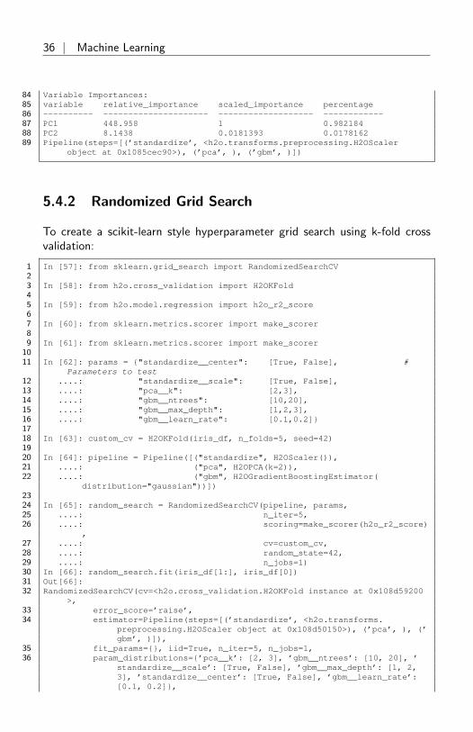
5.4.2 Randomized Grid Search

To create a scikit-learn style hyperparameter grid search using k-fold crossvalidation:

1 In [57]: from sklearn.grid_search import RandomizedSearchCV23 In [58]: from h2o.cross_validation import H2OKFold45 In [59]: from h2o.model.regression import h2o_r2_score67 In [60]: from sklearn.metrics.scorer import make_scorer89 In [61]: from sklearn.metrics.scorer import make_scorer

1011 In [62]: params = {"standardize__center": [True, False], #

Parameters to test12 ....: "standardize__scale": [True, False],13 ....: "pca__k": [2,3],14 ....: "gbm__ntrees": [10,20],15 ....: "gbm__max_depth": [1,2,3],16 ....: "gbm__learn_rate": [0.1,0.2]}1718 In [63]: custom_cv = H2OKFold(iris_df, n_folds=5, seed=42)1920 In [64]: pipeline = Pipeline([("standardize", H2OScaler()),21 ....: ("pca", H2OPCA(k=2)),22 ....: ("gbm", H2OGradientBoostingEstimator(

distribution="gaussian"))])2324 In [65]: random_search = RandomizedSearchCV(pipeline, params,25 ....: n_iter=5,26 ....: scoring=make_scorer(h2o_r2_score)

,27 ....: cv=custom_cv,28 ....: random_state=42,29 ....: n_jobs=1)30 In [66]: random_search.fit(iris_df[1:], iris_df[0])31 Out[66]:32 RandomizedSearchCV(cv=<h2o.cross_validation.H2OKFold instance at 0x108d59200

>,33 error_score=’raise’,34 estimator=Pipeline(steps=[(’standardize’, <h2o.transforms.

preprocessing.H2OScaler object at 0x108d50150>), (’pca’, ), (’gbm’, )]),

35 fit_params={}, iid=True, n_iter=5, n_jobs=1,36 param_distributions={’pca__k’: [2, 3], ’gbm__ntrees’: [10, 20], ’

standardize__scale’: [True, False], ’gbm__max_depth’: [1, 2,3], ’standardize__center’: [True, False], ’gbm__learn_rate’:[0.1, 0.2]},


37 pre_dispatch=’2*n_jobs’, random_state=42, refit=True,38 scoring=make_scorer(h2o_r2_score), verbose=0)3940 In [67]: print random_search.best_estimator_41 Model Details42 =============43 H2OPCA : Principal Component Analysis44 Model Key: PCA_model_python_1446220160417_1364546 Importance of components:47 pc1 pc2 pc348 ---------------------- -------- ---------- ----------49 Standard deviation 3.16438 0.180179 0.14378750 Proportion of Variance 0.994721 0.00322501 0.0020538351 Cumulative Proportion 0.994721 0.997946 1525354 ModelMetricsPCA: pca55 ** Reported on train data. **5657 MSE: NaN58 Model Details59 =============60 H2OGradientBoostingEstimator : Gradient Boosting Machine61 Model Key: GBM_model_python_1446220160417_1386263 Model Summary:64 number_of_trees model_size_in_bytes min_depth max_depth


------------ ------------ ------------ -------------66 20 2743 3 3 3

4 8 6.35676869 ModelMetricsRegression: gbm70 ** Reported on train data. **7172 MSE: 0.056674034632373 Rˆ2: 0.91679314687874 Mean Residual Deviance: 0.05667403463237576 Scoring History:77 timestamp duration number_of_trees training_MSE

training_deviance78 -- ------------------- ---------- ----------------- --------------

-------------------79 2015-10-30 09:04:46 0.001 sec 1 0.477453

0.47745380 2015-10-30 09:04:46 0.002 sec 2 0.344635

0.34463581 2015-10-30 09:04:46 0.003 sec 3 0.259176

0.25917682 2015-10-30 09:04:46 0.004 sec 4 0.200125

0.20012583 2015-10-30 09:04:46 0.005 sec 5 0.160051

0.16005184 2015-10-30 09:04:46 0.006 sec 6 0.132315

0.13231585 2015-10-30 09:04:46 0.006 sec 7 0.114554

0.114554


86 2015-10-30 09:04:46 0.007 sec 8 0.1003170.100317

87 2015-10-30 09:04:46 0.008 sec 9 0.08909030.0890903

88 2015-10-30 09:04:46 0.009 sec 10 0.08101150.0810115

89 2015-10-30 09:04:46 0.009 sec 11 0.07606160.0760616

90 2015-10-30 09:04:46 0.010 sec 12 0.07251910.0725191

91 2015-10-30 09:04:46 0.011 sec 13 0.06943550.0694355

92 2015-10-30 09:04:46 0.012 sec 14 0.067410.06741

93 2015-10-30 09:04:46 0.012 sec 15 0.06554870.0655487

94 2015-10-30 09:04:46 0.013 sec 16 0.06240410.0624041

95 2015-10-30 09:04:46 0.014 sec 17 0.06155330.0615533

96 2015-10-30 09:04:46 0.015 sec 18 0.0587080.058708

97 2015-10-30 09:04:46 0.015 sec 19 0.05792050.0579205

98 2015-10-30 09:04:46 0.016 sec 20 0.0566740.056674

99100 Variable Importances:101 variable relative_importance scaled_importance percentage102 ---------- --------------------- ------------------- ------------103 PC1 237.674 1 0.913474104 PC3 12.8597 0.0541066 0.0494249105 PC2 9.65329 0.0406157 0.0371014106 Pipeline(steps=[(’standardize’, <h2o.transforms.preprocessing.H2OScaler

object at 0x104f2a490>), (’pca’, ), (’gbm’, )])

References | 39

6 ReferencesH2O.ai Team. H2O website, 2016. URL http://h2o.ai

H2O.ai Team. H2O documentation, 2016. URL http://docs.h2o.ai

H2O.ai Team. H2O Python Documentation, 2015. URL http://h2o-release.s3.amazonaws.com/h2o/latest_stable_Pydoc.html

H2O.ai Team. H2O GitHub Repository, 2016. URL https://github.com/h2oai

H2O.ai Team. H2O Datasets, 2016. URL http://data.h2o.ai

H2O.ai Team. H2O JIRA, 2016. URL https://jira.h2o.ai

H2O.ai Team. H2Ostream, 2016. URL https://groups.google.com/d/forum/h2ostream

http://h2o.ai

http://docs.h2o.ai

http://h2o-release.s3.amazonaws.com/h2o/latest_stable_Pydoc.html

http://h2o-release.s3.amazonaws.com/h2o/latest_stable_Pydoc.html

https://github.com/h2oai

https://github.com/h2oai

http://data.h2o.ai

https://jira.h2o.ai



machine learning with python and h2o - amazon web … · machine learning with python and h2o ......

Documents