machine learning using stata/python

Cerulli G. (2020) #, # 1–22

Machine Learning using Stata/Python

Giovanni CerulliIRCrES-CNRRome, Italy

[email protected]

Abstract. We present two related Stata modules, r ml stata and c ml stata,for fitting popular Machine Learning (ML) methods both in a regression and aclassification setting. Using the recent Stata/Python integration platform (sfi)of Stata 16, these commands provide hyper-parameters’ optimal tuning via K-foldcross-validation using greed search. More specifically, they make use of the PythonScikit-learn API to carry out both cross-validation and outcome/label prediction.

Keywords: Machine Learning, Stata, Python, Optimal tuning

1 Introduction

Machine learning (ML) has emerged as a leading data science approach in many fields ofhuman activities, including business, engineering, medicine, advertisement, and scien-tific research. Placing itself in the intersection between statistics, computer science, andartificial intelligence, ML’s main objective is turning information into valuable knowl-edge by “letting the data speak”, limiting the model’s prior assumptions, and promotinga model-free philosophy. Relying on algorithms and computational techniques, morethan on analytic solutions, ML targets Big Data and complexity reduction, althoughsometimes at the expense of results’ interpretability (Hastie, Tibshirani, and Friedman,2001; Varian, 2014).

Unlike other software such as R, Python, Matlab, and SAS, Stata has not dedicatedbuilt-in packages for fitting ML algorithms, if one excludes the Lasso package of Stata16 (StataCorp, 2019). Recently, however, the Stata community has developed somepopular ML routines that Stata users can suitably exploit. Among them, we mentionSchonlau (2005) implementing a Boosting Stata plugin; Guenther and Schonlau (2016)providing a command fitting Support Vector Machines (SVM); Ahrens, Hansen, andSchaffer (2020) setting out the lassopack, a set of commands for model selection andprediction with regularized regression; and Schonlau and Zou (2020) recently providinga module for the random forest algorithm. All these are valuable packages to carry outpopular ML algorithms within Stata, but they lack uniformity and comparability asthey show up as stand–alone routines poorly integrated one another.

To pursuit generality, uniformity and comparability one should rely on a softwareplatform able to suitably integrate most of the mainstream ML methods. Python, forexample, has powerful platforms to carry out both ML and deep–learning algorithms(Raschka and Mirjalili, 2019). Among them, the most popular are Scikit–learn for fittinga large number of ML methods, and Tensorflow and Keras for fitting neural network and

© 2020

arX

iv:2

103.

0312

2v1

[st

at.C

O]

3 M

ar 2

021

2 Machine Learning in Stata

deep–learning techniques more in general. These make of Python, that is also a freewaresoftware, probably the most effective and complete software for ML and deep–learningavailable within the community.

The Stata 16 release has introduced a useful Stata/Python interface API, the StataFunction Interface (SFI) module, that allows users to interact Python’s capabilities withcore features of Stata. The module can be used interactively or in do–files and ado–files.

Using the Stata/Python integration interface, this paper presents two related Statamodules, r ml stata and c ml stata wrapping Python functions for fitting popularMachine Learning (ML) methods both in a regression and a classification setting. Bothcommands provide hyper-parameters’ optimal tuning via K–fold cross–validation byimplementing greed search. More specifically, they make use of the Python Scikit-learnAPI to carry out both cross-validation and outcome/label prediction.

Why the Stata community would need these commands? I see three related answersto this question. First, Stata users who are willing to apply ML methods would benefitfrom these commands as they can allow them to perform ML without time–consuminginvestment in learning other software. Second, these commands provide users withstandard Stata returns and variables’ generation that can be further used in subsequentStata coding within the same do–file. This makes the user’s workflow smoother, lesserror-prone, and faster. Third, these commands represent a sort of a case–study show-ing the potential of integrating Stata and Python. To my experience, indeed, Stata isunbeatable compared to Python when it comes to performing intensive data manage-ment and manipulation, descriptive statistics, and immediate graphing, while Python ismore suitable for its large set of implemented ML algorithms, for an all–encompassingavailability of libraries, for computing speed and sophisticated graphing (not only 3D,but also deep contour plots, and images’ reproduction).

The structure of the paper is as follows. Section 2 presents a brief introduction tomachine learning, where subsection 2.1 sets out the basics, subsection 2.2 the optimaltuning procedure via cross-validation, and subsection 2.3 the learning methods andarchitecture. Section 3.1 and 3.2 present the syntax of r ml stata and c ml stata.For users to familiarize with these commands, section 4 illustrates a simple step–by–step application for fitting a regression tree, while sections 5 and 6 show how to applythe previous commands to a real dataset for either classification and regression purposes.Section 7 concludes the paper.

2 A brief introduction to machine learning

2.1 The basics of machine learning

Machine learning is the branch of artificial intelligence mainly focused on statisticalprediction (Boden, 2018). The literature distinguishes between supervised and unsu-pervised learning, referring to a setting where the outcome variable is known (super-vised) or unknown (unsupervised). In statistical terms, supervised learning coincides

Giovanni Cerulli 3

with a regression or classification setup, where regression represents the case in whichthe outcome variable is numerical, and classification the case in which it is categorical.In contrast, unsupervised learning deals with unlabeled data, and its main concern isthat of generating a categorical variable via proper clustering algorithms. Unsupervisedlearning can thus be encompassed within statistical cluster analysis.

In this article, we focus on supervised machine learning1. We are thus interestedin predicting either numerical variables (regression) or label classes (classification) asa function of p predictors (or features) that may be both quantitative or qualitative.From a statistical point of view, we want to fit the conditional expectation of Y , theoutcome, on a set of p predictors, X, starting from the following population equation:

Y = f(X1, . . . , Xp) + ε (1)

where ε is an error term with mean equal to zero and finite variance. By taking theexpectation over X, and assuming that E(ε|X) = 0, we have:

Y = E(Y |X) + ε = f(X1, . . . , Xp) + ε (2)

that is:E(Y |X) = f(X1, . . . , Xp) (3)

The conditional expectation f(·) represents a function mapping predictors and expectedoutcomes. The main purpose of supervised machine learning is that of fitting Eq. (3)with the aim of reducing as much as possible the prediction error coming up when onewants to predict actual outcome variables. The prediction error can be generally definedas e = Y − f(X), with f(·) indicating a specific ML method. Generally, ML scholars

focus on minimizing the mean square error (MSE), defined as MSE = E[Y − f(X)]2.However, while the in–sample MSE (the so–called “training–MSE”) is generally affectedby overfitting (thus going to zero as the model’s degrees of freedom - or complexity -raises up), the out–of–sample MSE (also known as “test-MSE”) has the property to bea convex function of model complexity, and thus characterized by an optimal level ofcomplexity.

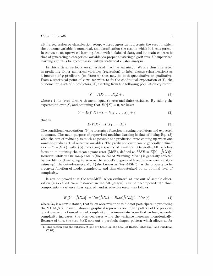
It can be proved that the test-MSE, when evaluated at one out–of–sample obser-vation (also called “new instance” in the ML jargon), can be decomposed into threecomponents – variance, bias squared, and irreducible error – as follows:

E[(Y − f(X0)]2 = V ar(f(X0) + [Bias(f(X0)]2 + V ar(ε) (4)

where X0 is a new instance, that is, an observation that did not participate in producingthe ML fit f(·). Figure 1 shows a graphical representation of the pattern of the previousquantities as functions of model complexity. It is immediate to see that, as long as modelcomplexity increases, the bias decreases while the variance increases monotonically.Because of this, the test–MSE sets out a parabola-shaped pattern which allows us for

1. This section and the subsequent one are based on the book of Hastie, Tibshirani, and Friedman(2001).


minimizing it at a specific level of model complexity. This is the optimal model tuningwhenever complexity is measured by a specific hyper-parameter λ. In the figure, theirreducible error variance represents a constant lower bound of the test–MSE. It is notpossible to overcome this minimum test–MSE, as it depends on the nature of the datagenerating process (intrinsic unpredictability of the phenomenon under analysis).

Figure 1: Trade-off between bias and variance as functions of model complexity.

In the classification setting, the MSE is meaningless as in this case we have class la-bels and not numerical values. For classification purposes, the correct objective functionto minimize is the (test) mean classification error (MCE) defined as:

MCE = E[I(y 6= C(X))] (5)

where I(·) is an index function, and C(X) the fitted classifier. As in the case of theMSE, it can be proved that the training–MCE overfits the data when model complexityincreases, while the test–MCE allows us to find the optimal model’s complexity. There-fore, the graph of figure 1 can be likewise extended also to the case of the test–MCE.

2.2 Optimal tuning via cross-validation

Finding the optimal model complexity, parameterized by a generic hyper–parameter λ,is a computational task. There are basically three ways to tune an ML model:

Giovanni Cerulli 5

• Information criteria

• K–fold cross–validation

• Bootstrap

Information criteria are based on goodness–of–fit formulas that adjust the trainingerror by penalizing too complex models (i.e., models characterized by large degrees offreedom). Traditional information criteria comprise the Akaike criterion (AIC) and theBayesian information criterion (BIC), and can be applied to both linear and non–linearmodels (probit, logit, poisson, etc.). Unfortunately, the information criteria are validonly for linear or generalized linear models, i.e. for parametric regression. They cannotbe computed for nonparametric methods like – for example – tree–based or nearestneighbor regressions.

For nonparametric models, the test–error can be estimated via computational tech-niques, more specifically, by resampling methods. Boostrap – resampling with replace-ment from the original sample – could in theory be a practical solution, provided thatthe original dataset is used as validation dataset and the bootstrapped ones as train-ing datasets. Unfortunately, the bootstrap has the limitation of generating observationoverlaps between the test and the training datasets, as about two-thirds of the originalobservations appear in each bootstrap sample. This occurrence undermines its use tovalidate out–of–sample an ML procedure.

Cross–validation is the workhorse of the test–error estimation in machine learning.The idea is to randomly divide the initial dataset into K equal–sized portions calledfolds. This procedure suggests to leave out fold k and fit the model to the other (K-1)folds (wholly combined) to then obtain predictions for the left-out k–th fold. This is donein turn for each fold k = 1, 2, . . . ,K, and then the results are combined by averagingthe (K-1) estimates of the error. The cross–validation procedure can be carried out asfollows:

• Split randomly the initial dataset into K folds denoted as G1, G2, . . . , GK , whereGk refers to part k. Assume that there are nk observations in fold k. If N is amultiple of K, then nk = n/K.

• For each fold k = 1, 2, . . . ,K, compute:

MSEk =∑i∈Ck

(yi − yi)2/nk

where yi is the fit for observation i, obtained from the dataset with fold k removed.

• Compute:

CVK =

K∑i=1

nknMSEk

that is the average of all the out–of–sample MSE obtained fold–by–fold.


ML method Parameter 1 Parameter 2 Parameter 3

Linear Models and GLS N. of covariatesLasso Penalization coefficientElastic-Net Penalization coefficient Elastic parameterNearest-Neighbor N. of neighborsNeural Network N. of hidden layers N. of neuronsTrees N. of leavesBoosting Learning parameter N. of bootstraps N. of leavesRandom Forest N. of features for splitting N. of bootstraps N. of leavesBagging Tree-depth N. of bootstrapsSupport Vector Machine C ΓKernel regression Bandwidth Kernel functionPiecewise regression N. of knotsSeries regression N. of series terms

Table 1: Main machine learning methods and associated tuning hyper–parameters.

Observe that, by setting K = n, we obtain the n–fold or leave-one out cross-validation(LOOCV). Also, as CVK is an estimation the true test–error, estimating its standarderror can be useful to provide a confidence interval and thus a measure of test–accuracy’suncertainty.

For ML classification purposes, finally, the cross-validation procedure follows thesame line, except for considering the MCE in place of the MSE.

2.3 Learning methods and architecture

A learner Lj is a mapping from the set [X, θ, λj , fj(·)] to an outcome y, where X is thematrix of features, θ a vector of estimation parameters, λj a vector of tuning parameters,and fj(·) an algorithm taking as inputs X, θ, and λj . Differently from the members ofthe Generalized Linear Models (GLM) family (linear, probit or multinomial regressionsare classical examples), that are highly parametric and are not characterized by tuningparameters, machine learning models – such as local–kernel, nearest–neighbor, or tree–based regressions – may be highly nonparametric and characterized by one or morehyper-parameters λj which may be optimally chosen to minimize the test predictionerror, i.e. the out–of–sample predicting accuracy of the learner, as stressed in theprevious section.

A detailed description of all the available machine learning methods is beyond thescope of this paper. Table 1, however, sets out the most popular machine learning algo-rithms proposed in the literature along with the associated tuning hyper–parameters.

A combined use of these methods can produce a computational architecture (i.e., avirtual learning machine) enabling to increase statistical prediction and its estimatedprecision (Van der Laan, Polley and Hubbard, 2007). Figure 2 presents the learning

Giovanni Cerulli 7

architecture proposed by Cerulli (2020). This framework is made of three linked learn-ing processes: (i) the learning over the tuning parameter λ, (ii) the learning over thealgorithm f(·), and (iii) the learning over new additional information. The departure isin point 1, from where we set off assuming the availability of a dataset [X, y].

The first learning process aims at selecting the optimal tuning parameter(s) for agiven algorithm fj(·). As seen above, ML scholars typically do it using K-fold cross–validation to draw test–accuracy (or, equivalently, test–error) measures and relatedstandard deviations.

Figure 2: The meta–learning machine architecture.

At the optimal λj , one can recover the largest possible prediction accuracy for thelearner fj(·). Further prediction improvements can be achieved only by learning fromother learners, namely, by exploring other fj(·), with j = 1, . . . ,M (where M is thenumber of learners at hand).

Figure 1 shows the training estimation procedure that corresponds to the light bluesequence of boxes leading to the MSETRAIN which is, de facto, a dead-end node, beingthe training error plagued by overfitting.

Conversely, the yellow sequence leads to the MSETEST , which is informative totake correct decisions about the predicting quality of the current learner. At this node,the analyst can compare the current MSETEST with a benchmark one (possibly, pre–fixed), and conclude whether to predict using the current learner, or explore alternativelearners in the hope of increasing predictive performance. If the level of the currentprediction error is too high, the architecture would suggest to explore other learners.


In the ML literature, learning over learners is called meta learning, and entails anexploration of the out–of–sample performance of alternative algorithms fj(·) with thegoal of identifying one behaving better than the those already explored (Van der Laanand Rose, 2011). For each new fj(·), our architecture finds an optimal tuning parameterand a new estimated accuracy (along with its standard deviation). The analyst caneither explore the entire bundle of alternatives and finally pick–up the best one, ordecide to select the first learner whose accuracy is larger than the benchmark. Eithercases are automatically run by this virtual machine.

The third final learning process concerns the availability of new information, viaadditional data collection. This induces a reiteration of the initial process whose finaloutcome can lead to choose a different algorithm and tuning parameter(s), dependingon the nature of the incoming information.

As final step, one may combine predictions of single optimal learners into one singlesuper–prediction (ensemble learning). What is the advantage of this procedure? As anaverage, this method cannot provide the largest accuracy possible. However, as sumsof i.i.d. random variables have smaller variance than the single addends, the benefitconsists of a smaller predictive uncertainty (Zhou, 2012).

3 Syntax

3.1 Syntax for r ml stata

The command r ml stata fits machine learning regression algorithms. It considers asthe main inputs a continuous response variable y (i.e. the depvar), a series of predictors(or features) in varlist explaining the y, plus a series of options.

r ml stata depvar varlist , mlmodel(modeltype) out sample(filename)

in prediction(name) out prediction(name) cross validation(name)

seed(integer)[, save graph cv(name)

]depvar is a numerical variable. Missing values are not allowed.

varlist is a list of numerical variables representing the features. When a feature iscategorical, please generate the categorical dummies related to this feature. Asthe command does not do it by default, it is user’s responsibility to generate theappropriate dummies. Missing values are not allowed.

Options

mlmodel(modeltype) specifies the machine learning algorithm to be estimated. model-type takes the following options: elasticnet (Elastic–net), tree (Regression tree),randomforest (Bagging and Random forests), boost (Boosting), nearestneighbor(Nearest Neighbor), neuralnet (Neural network), svm (Support vector machine).

Giovanni Cerulli 9

out sample(filename) requests to provide a new dataset in filename containing the newinstances over which estimating predictions. This dataset contains only features.

in prediction(name) requires to specify a name for the file that will contain in–samplepredictions.

out prediction(name) requires to specify a name for the file that will contain out–sample predictions, those obtained from the option out sample(filename).

cross validation(name) requires to specify a name for the dataset that will containcross–validation results. The command uses K–fold cross–validation, with K=10 bydefault.

seed(integer) requests to specify a integer seed to assure replication of same results.

save graph cv(name) allows to obtain the cross-validation optimal tuning graph draw-ing the pattern of both train and test accuracy.

Returns

r ml stata returns into e-return scalars (if numeric) or macros (if string) the “optimalhyper-parameters”, the “optimal train accuracy”, the “optimal test accuracy”, andthe “standard error of the optimal test accuracy” obtained via cross–validation.

Remarks

Missing values in both the outcome and the list of features are not allowed. Beforerunning this command, please check whether your dataset presents missing valuesand delete them.

To run this program you need to have both Stata 16 and Python (from version 2.7onwards) installed. Also, the Python packages Scikit-learn, Pandas, Numpy, andScipy must be installed before running the command.

3.2 Syntax for c ml stata

The command c ml stata fits machine learning classification algorithms. It considers asthe main inputs a categorical response variable y (i.e. the depvar), a series of predictors(or features) in varlist explaining the y, plus a series of options.

c ml stata depvar varlist , mlmodel(modeltype) out sample(filename)

in prediction(name) out prediction(name) cross validation(name)

seed(integer)[, save graph cv(name)

]depvar is a numerical discrete dependent variable representing the different classes. It

is recommended to re–code this variable so to take values [1, 2, ...,M ] in a M -classsetting. For example, if the outcome is binary taking values [0, 1], remember to


record it so to take values [1, 2]. Missing values are not allowed.

varlist is a list of numerical variables representing the features. When a feature iscategorical, please generate the categorical dummies related to this feature. Asthe command does not do it by default, it is user’s responsibility to generate theappropriate dummies. Missing values are not allowed.

Options

mlmodel(modeltype) specifies the machine learning algorithm to be estimated. mod-eltype takes the following options: tree (Tree-based classification), randomforest(Bagging and Random forests), boost (Boosting), regularizedmultinomial (Reg-ularized multinomial), nearestneighbor (Nearest neighbor), neuralnet (Neuralnetwork), naivebayes (Naıve Bayes), svm (Support vector machine).

out sample(filename) requests to provide a new dataset in filename containing the newinstances over which estimating predictions. This dataset contains only features.

in prediction(name) requires to specify a name for the file that will contain in–samplepredictions.

out prediction(name) requires to specify a name for the file that will contain out–sample predictions, those obtained from the option out sample(filename).

cross validation(name) requires to specify a name for the dataset that will containcross–validation results. The command uses K–fold cross–validation, with K=10 bydefault.

seed(integer) requests to specify a integer seed to assure replication of same results.

save graph cv(name) allows to obtain the cross-validation optimal tuning graph draw-ing the pattern of both train and test accuracy.

Returns

c ml stata returns into e-return scalars (if numeric) or macros (if string) the “optimalhyper-parameters”, the “optimal train accuracy”, the “optimal test accuracy”, andthe “standard error of the optimal test accuracy” obtained via cross-validation.

c ml stata provides model predictions both as predicted labels and as predicted prob-abilities.

Remarks

Missing values in both outcome and varlist are not allowed. Before running this com-mand, please check whether your dataset presents missing values and delete them.

To run this program you need to have both Stata 16 and Python (from version 2.7onwards) installed. Also, the Python packages Scikit-learn, Pandas, Numpy, and

Giovanni Cerulli 11

Scipy must be installed before running the command.

4 Application 1: fitting a regression tree

This section presents an illustrative application of the use of both r ml stata within across–section data structure. It is thought to allow users to become familiar with theuse of this module (the use of c ml stata follows a similar procedure). To begin with,I show how to implement step–by–step a regression tree.

• Step 1. Before starting, install Python (from version 2.7 onwards), and thePython packages Scikit--learn, Numpy, Pandas, and Scipy. If you need a helpon how to install Python and its packages look at the Python webpage2.

• Step 2. Once you have Python installed in your machine, you need to install theStata ML command:

. ssc install r_ml_stata

and look at the documentation file of the command to explore its syntax:

. help r_ml_stata

• Step 3. The command requires to provide a dataset with no missing values. It isuser’s responsibility to assure this. We can thus load the training dataset preparedfor this example:

. use "r_ml_stata_data_example"

This dataset contains one target variable (y) and 13 features (x1, x2, ..., x13). Allvariables are numerical and thus suitable for running our regression tree.

Before running the command, however, a testing dataset must be provided. Thisis a dataset made of the same features of the training one, but with new in-stances. Observe that this dataset must neither contain missing values, nor in-clude the target variable (y). In this example, we prepared a testing dataset calledr ml stata data new example. This dataset must be in the same directory of thetraining dataset.

• Step 4. There are now all the ingredients to run our regression tree. We simplyrun these lines of code in Stata:

. r_ml_stata y x1-x13 , mlmodel(tree) in_prediction("in_pred") ///cross_validation("CV") out_sample("r_ml_stata_data_new_example") ///out_prediction("out_pred") seed(10) save_graph_cv("graph_cv")

where the syntax has this meaning:

– The argument tree tells Stata to run a tree–regression. Other options areavailable (see the help-file).

2. Specifically, look at the Python installation page: https://realpython.com/installing-python.


– The argument in pred tells Stata to generate a dataset in pred.dta con-taining the in–sample predictions of the estimated model. They are thepredictions for only the training dataset.

– The argument out pred tells Stata to generate a dataset out pred.dta con-taining the out–of–sample predictions of the estimated model. They arepredictions only for the testing dataset.

– The argument r ml stata data new example tells Stata to use this one astesting dataset.

– The seed is necessary to replicate the same results and must be an integer.

– The argument graph cv tells Stata to save the cross–validation results graphin your current directory.

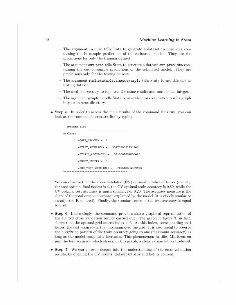
• Step 5. In order to access the main results of the command thus run, you canlook at the command’s ereturn list by typing:

. ereturn list---------------------------------------scalars:

e(OPT_LEAVES) = 4

e(TEST_ACCURACY) = .2027650052251946

e(TRAIN_ACCURACY) = .8911061692860425

e(BEST_INDEX) = 3

e(SE_TEST_ACCURACY) = .742518604039193---------------------------------------

We can observe that the cross–validated (CV) optimal number of leaves (namely,the tree optimal final nodes) is 4, the CV optimal train accuracy is 0.89, while theCV optimal test accuracy is much smaller, i.e. 0.20. The accuracy measure is theshare of the total outcome variance explained by the model (it is closely similar toan adjusted R-squared). Finally, the standard error of the test accuracy is equalto 0.74.

• Step 6. Interestingly, the command provides also a graphical representation ofthe 10–fold cross–validation results carried out. The graph in figure 3, in fact,shows that the optimal grid search index is 3. At this index, corresponding to 4leaves, the test accuracy is the maximum over the grid. It is also useful to observethe overfitting pattern of the train accuracy going to one (maximum accuracy) aslong as the model complexity increases. This phenomenon justifies ML focus onjust the test accuracy which shows, in this graph, a clear variance–bias trade–off.

• Step 7. We can go even deeper into the understanding of the cross-validationresults, by opening the CV results’ dataset CV.dta and list its content:

Giovanni Cerulli 13

Figure 3: Cross-validation graph for a tree regression.

. use CV , clear

. list

+--------------------------------------------+| index mean_tr~e mean_tes~e std_tes~e ||--------------------------------------------|

1. | 0 .46707705 -.06167094 .39788509 |2. | 1 .70630139 .19044095 .4556592 |3. | 2 .82658573 .0736554 .81239835 |4. | 3 .89110617 .20276501 .7425186 |5. | 4 .9226751 .03514619 1.106288 |

|--------------------------------------------|6. | 5 .94706553 .05360043 .80043332 |7. | 6 .9643006 .08797992 .8920612 |8. | 7 .97651532 .03100165 .89505782 |9. | 8 .98468366 -.10475403 .99490224 |

10. | 9 .99037207 .04775965 .91827191 ||--------------------------------------------|

11. | 10 .99419849 -.10484366 .98651178 |12. | 11 .99669445 -.20313959 1.2912981 |13. | 12 .99800409 -.10410404 .97689497 |


14. | 13 .99881627 .07493419 .85811843 |15. | 14 .99929196 -.03926511 .91545614 |

+--------------------------------------------+

Results show, by every grid index, the train accuracy, the test accuracy, and thestandard error of the test accuracy estimated over the 10–fold runs. The standarderror is important, as it measures the precision we obtain when estimating thetest accuracy. In this example, at the optimal index (i.e., 3), the test accuracy’sstandard error is 0.74, which should be compared with those obtained from otherML algorithms. This means that the choice of the ML model to employ forprediction purposes should ponder not only the level of the achieved test accuracy,but also its standard error.

• Step 8. Finally, we can have a look at the out-of-sample predictions. This canbe done by opening and listing the out pred dataset:

. use out_pred , clear

. list

+-------------------+| index out_sam~d ||-------------------|

1. | 0 21.629744 |2. | 1 16.238961 |3. | 2 21.629744 |4. | 3 16.238961 |5. | 4 16.238961 |

|-------------------|6. | 5 16.238961 |7. | 6 16.238961 |8. | 7 16.238961 |9. | 8 16.238961 |

10. | 9 21.629744 ||-------------------|

11. | 10 27.427273 |+-------------------+

We observe that the predictions are made of only three values [21.62, 16.23, 27.42]corresponding to three out of the four optimal terminal tree leaves. Graphicallyit represents a step–function (omitted for the sake of brevity).

5 Application 2: ML classification

In this section, we show an illustrative application of c ml stata using the popularauto dataset. We intend to guess whether a “new” car is a “foreign” or “domestic” onebased on a series of characteristics, including price, number of repairs, weight, etc. Ourgoal is to provide a comparison of the accuracy performed by the classifiers availablethrough c ml stata. This is in tune with the learning architecture outlined in section2.3, as it can provide guidance over the choice of the proper learner to use. In order to

Giovanni Cerulli 15

carry out this analysis, we proceed in three steps: the first bunch of code cleans andprepares the datasets (training and test) to use for fitting c ml stata in a correct way;the second bunch of code fits all the learners available to the data; a third and final partof the code yields a forest plot for visualizing and comparing learners’ test accuracy andstandard deviation.

We start by setting out the code for data cleaning and preparation:

********************************************************************************* DATA CLEANING AND PREPARATION********************************************************************************* Clean the detaset eliminating all labels and missing valuesclear allcd "/Users/giocer/Dropbox/Stata_Python/Paper_c_r_ml_stata"sysuse auto , clearlabel drop _alldrop makequi reg _allkeep if e(sample)

* Standardize the featuresglobal X "price mpg rep78 headroom trunk weight length turn displacement gear_ratio"global XX ""foreach V of global X{egen ‘V’_std=std(‘V’)drop ‘V’rename ‘V’_std ‘V’global XX $XX ‘V’}

* Recode the binary target variablerecode foreign (0=1) (1=2)

* Save the initial datasetsave mydata , replace

* Split the initial dataset into a "training" and a "test" datasetsplitsample, generate(svar, replace) split(0.15 0.85) rseed(1) show

* Save the the training dataset as "data_train.dta"preservekeep if svar==2drop svarsave data_train , replacerestore

* Save the the test dataset as "data_test.dta"preservekeep if svar==1drop foreign svarsave data_test , replacerestore********************************************************************************

The outputs of this first part of the code are two datasets obtained through a randomsplit of the initial auto dataset, data train used for in–sample fit, and data test usedfor out–of–sample classification. It is important to bear in mind that the data test

must contain only the (standardized) features, while both need to be without labels and


missing values.

In the second part of the code, we fit the learners to the training dataset. We performthis task by looping over the global LEARNERS that contains the name of the classifiersallowed by c ml stata.

********************************************************************************* FITTING ML CLASSIFIERS********************************************************************************* Define global macros Y, X, and LEARNERS for the fittingglobal Y "foreign"global X $XXglobal LEARNERS tree randomforest boost ///regularizedmultinomial nearestneighbor ///neuralnet naivebayes svm"

* Define a matrix M that will contain the main resultslocal i=1global m: word count $LEARNERSmat M=J($m,3,.)

* Fit all the ML methods by a loop over "LEARNERS" and save the main fitting* results into the matrix Mforeach L of global LEARNERS{* Load the training datasetuse data_train , clear* Fit the single learnerc_ml_stata $Y $X , mlmodel(‘L’) in_prediction("in_pred_‘i’") cross_validation("CV_‘i’") ///out_sample("data_test") out_prediction("out_pred_‘i’") seed(10) save_graph_cv("graph_cv_‘i’")* Save results into Mmat M[‘i’,1]=e(TRAIN_ACCURACY)mat M[‘i’,2]=e(TEST_ACCURACY)mat M[‘i’,3]=e(BEST_INDEX)mat colnames M = TRAIN_ACCURACY TEST_ACCURACY indexmat rownames M = ‘L’local i=‘i’+1}

* Turn the information contained in M into a dataset called "RES.dta"clearsvmat M , n(col)gen Learner=""local i=1foreach L of global LEARNERS{replace Learner="‘L’" in ‘i’local i=‘i’+1}replace index=int(index)save RES , replace

* Put all the cross-validation graphs into a global macro called "TOT"global TOT ""forvalues i=1/8{global TOT $TOT graph_cv_‘i’.gph}

* Combine the graphs export the final graphgraph combine $TOT , scale(*0.5) plotregion(style(none)) scheme(s1mono)graph export cv_graph_all.png , as(png) replace

Giovanni Cerulli 17

********************************************************************************

The main outputs of this part are in the dataset RES containing, for every learner,the optimal greed index, the training and test accuracy, and the graph cv graph all

displaying the cross–validation maximum of the classification test accuracy (i.e., theminimum of the classification error) over a greed of learners’ tuning parameters. Thisgraph is visible in figure 4.

Figure 4: Cross–validation maximum of the classification test accuracy over a greed oflearners’ tuning parameters. Accuracy measure: “error rate” (taking values betweenzero and one).

********************************************************************************* FOREST PLOT FOR LEARNERS’ ACCURACY********************************************************************************* Build a Forest Plot of the accuracy by Learner: mean & standard deviationclearglobal LEARNERS tree randomforest boost ///regularizedmultinomial nearestneighbor ///neuralnet naivebayes svmglobal CV ""forvalues i=1/8{use CV_‘i’


local L: word ‘i’ of $LEARNERScap drop Learnergen Learner="‘L’"save CV_‘i’ , replaceglobal CV $CV CV_‘i’}********************************************************************************clearappend using $CVtab Learner , mis********************************************************************************merge 1:1 index Learner using RESkeep if _merge==3sort Learner********************************************************************************sum mean_test_scoreglobal MEAN=r(mean)********************************************************************************replace Learner="Boosting" in 1replace Learner="Naive Bayes" in 2replace Learner="Nearest neighbor" in 3replace Learner="Neural network" in 4replace Learner="Random forest" in 5replace Learner="Regularized multinomial" in 6replace Learner="Support vector machine" in 7replace Learner="Tree" in 8********************************************************************************cap drop Cgen C=‘"""’cap drop Agen A=_ntostring A,replacecap drop _Lgen _L= A + " " + C + Learner + C********************************************************************************levelsof _L , local(XX) cleanglobal XX ‘XX’********************************************************************************cap drop _idgen _id=_ncap drop logen lo=mean_test_score-1.96*std_test_scorecap drop higen hi=mean_test_score+1.96*std_test_score********************************************************************************format mean_test_score %12.2g********************************************************************************twoway (rcap lo hi _id , horizontal ) (scatter _id mean_test_score , ///msymbol(S) msize(small) mcolor(black) mlabel(mean_test_score) ///mlabposition(12) mlabc(red) mlabs(medlarge)) , ylabel($XX , angle(0)) ytitle("") ///plotregion(style(none)) scheme(s1mono) xtitle("") legend(off) ///xline($MEAN , lc(orange) lpattern(dash) lw(medthick) ) xtitle(Test accuracy)graph export forestplot.png , as(png) replace********************************************************************************

The first part of this code extracts from the cross-validation results (contained, for ev-ery learner, in the dataset CV ) the standard error of the test accuracy. The resultingdataset is then merged with the RES dataset, thus allowing for plotting mean and stan-dard deviation of each learner’s test accuracy within a forest plot. This graph is visible

Giovanni Cerulli 19

in figure 5. The results clearly show that in this dataset the neural network performsparticularly well, with a cross–validation test accuracy of 0.97 and the smallest confi-dence interval. One contrary, classification tree perform poorly, with a test accuracy of0.85 and a large confidence interval. The other classifiers perform within this range andgenerally set out rather large confidence intervals.

Figure 5: Forest plot for comparing mean and standard deviation of different learners.Classification setting.

6 Application 3: ML regression

In this application, we present the results from running a regression predictive analysisusing r ml stata. For the sake of brevity, we do not report the code as it is identicalto the one of the classification exercise, except for choosing as target the continuousvariable price instead of the binary foreign (now included in the model as feature).

The cross–validation results are visible in figure 6 showing the greed index maxi-mizing the test prediction accuracy. For regression, the selected accuracy measure isthe prediction “explained variance” that takes a maximum value of one in the case of


perfect prediction.

Figure 6: Cross–validation maximum of the regression test accuracy over a greed oflearners’ tuning parameters. Accuracy measure: “explained variance” (taking one asmaximum value).

Figure 7 sets out the comparison among the different learners computed by r ml stata

in terms of the mean accuracy and standard deviation. Similarly to the classificationcase, we can observe that the learners behave differently, with boosting showing thebest mean test accuracy (0.49) and tighter confidence interval. The worst performinglearner is the nearest neighbor, both in term of mean accuracy and standard deviation.

7 Conclusion

In the last two decades, advances in statistical learning and computation have radicallyimproved the prediction performance of targeted outcomes in pretty all scientific do-mains, including engineering, robotics, and artificial intelligence. ML has emerged as anew scientific paradigm to model outcomes and design pragmatic architectures for rea-soned decision–making in uncertain environments. Thanks to the recent Stata/Python

Giovanni Cerulli 21

Figure 7: Forest plot for comparing mean and standard deviation of different learners.Regression setting.

integration platform introduced within Stata 16, producing Stata routines able to fit MLregression and classification has become a relatively straightforward task. By exploit-ing this opportunity, this paper has presented two related Stata modules, r ml stata

and c ml stata, for fitting popular ML models both in a regression and a classificationsetting. These commands provide hyper-parameters’ optimal tuning via K-fold cross-validation using greed search, by wrapping the Python Scikit-learn API to performcross-validation and outcome/label prediction.

Compared to other popular statistical software, Stata has the advantage to be highlyuser–friendly and powerful for complex data management. Unfortunately, Stata has notyet embedded a built-in Machine Learning package, except for the Lasso (including alsothe Elastic-net).

The two commands herein presented thus go in the direction to partly fill this gap byproviding the Stata users with two simple but powerful commands for fitting various MLmethods. Further development of this work may include to provide also deep–learningStata routines by wrapping into Stata the Python platforms Keras and Tensorflow.


8 ReferencesAhrens A., Hansen C.B., Mark E. Schaffer M.E. 2020. lassopack: Model selection and

prediction with regularized regression in Stata, The Stata Journal, 20(1):176-235.

Boden M.A. 2018. Artificial Intelligence: A Very Short Introduction, Oxford UniversityPress.

Cerulli G. 2020. Improving econometric prediction by machine learning, Applied Eco-nomics Letters, forthcoming.

Guenther N., Schonlau M. 2016. Support Vector Machines, The Stata Journal, 16(4)917-937.

Hastie T., Tibshirani R., and Friedman J. 2001. The elements of Statistical Learning -Data Mining, Inference, and Prediction. Berlin: Springer-Verlag.

Raschka, S., Mirjalili, V. 2019. Python Machine Learning. 3rd Edition, Packt Publishing.

Schonlau M. 2005. Boosted Regression (Boosting): An Introductory Tutorial and aStata Plugin, The Stata Journal, 5(3):330-354.

Schonlau M., Zou R.Y. 2020. The random forest algorithm for statistical learning. TheStata Journal, 20(1):3-29.

StataCorp. 2019. Stata 16 Lasso Reference Manual. College Station, TX: Stata Press.

Van der Laan, M., Polley E.C., and Hubbard A.E.. 2007. Super Learner, StatisticalApplications in Genetics and Molecular Biology, 6(1).

Van der Laan M.J. and Rose S. 2011. Targeted learning: causal inference for observa-tional and experimental data. Springer.

Varian H.R. 2014. Big Data: New Tricks for Econometrics. Journal of Economic Per-spectives, 28(2): 3-28.

Zhou Z.H. 2012. Ensemble Methods: Foundations and Algorithms. CRC Press.

machine learning using stata/python

Documents