machine learning: topic chart - ethz - home · pdf filemachine learning: topic chart ......

Machine Learning: Topic Chart

• Core problems of pattern recognition

• Bayesian decision theory

• Perceptrons and Support vector machines

• Data clustering

• Dimension reduction

Visual Computing: Joachim M. Buhmann — Machine Learning 268/290

What is Dimensionality Reduction ?

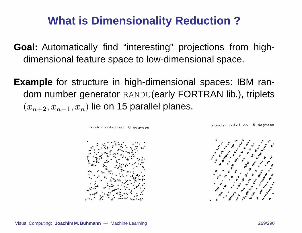
Goal: Automatically find “interesting” projections from high-dimensional feature space to low-dimensional space.

Example for structure in high-dimensional spaces: IBM ran-dom number generator RANDU(early FORTRAN lib.), triplets(xn+2, xn+1, xn) lie on 15 parallel planes.


Reasons for Dimensionality Reduction

select most interesting dimensions in preprocessing step:

• data compression• feature selection• complexity reduction

• Example: face recognition, m×n grey-scale image lives inmn-dimensional space.

visualization of data: project to 1, 2 or 3 dimensional space.


When does Dimensionality Reduction work?

“Noise dimensions”: many variables may have very small va-riation, and may hence be ignored

Decoupling: many variables may be correlated / dependent,hence a new set of independent variables is preferable.

Problem: projection is “smoothing”: (high-dim.) structure isobscured, but never enhanced.

Goal: find sharpest / most interesting projections


linear vs. non-linear projections

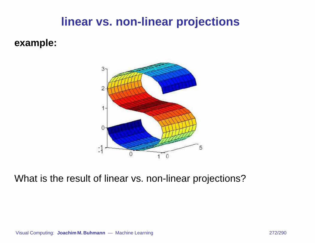
example:

What is the result of linear vs. non-linear projections?


Overview

Linear Projections:

• Principal Component Analysis (PCA)• Exploratory Projection Pursuit

Non-Linear Projections:

• locally linear embedding (LLE)• more methods in “Machine Learning II”


Linear Projection

from high-dim. space Rd to low-dim. space Rm:

z = Wx

wherex ∈ Rd

z ∈ Rm

W is a linear map (matrix):

• orthogonal projection: row vectors of W are orthonormal• if m = 1: W reduces to a row vector w>

Note: while the projection is linear, the objective function (seebelow) may be non-linear!


Principal Component Analysis (PCA)

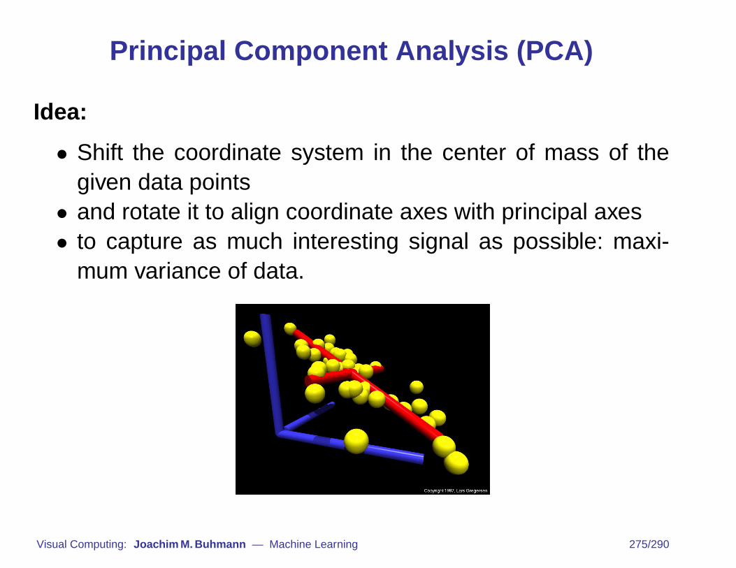
Idea:

• Shift the coordinate system in the center of mass of thegiven data points

• and rotate it to align coordinate axes with principal axes• to capture as much interesting signal as possible: maxi-

mum variance of data.


PCA: formal setup

Given are data points xs ∈ Rd, s = 1, ..., n.

New Rotated Coordinate System: Define a new set of d or-thonormal basis vectors φi ∈ Rd, i.e.,

φ>i φj =

{1 for i = j

0 otherwise

data point in new coordinate system: xs =d∑

i=1

ysi φi


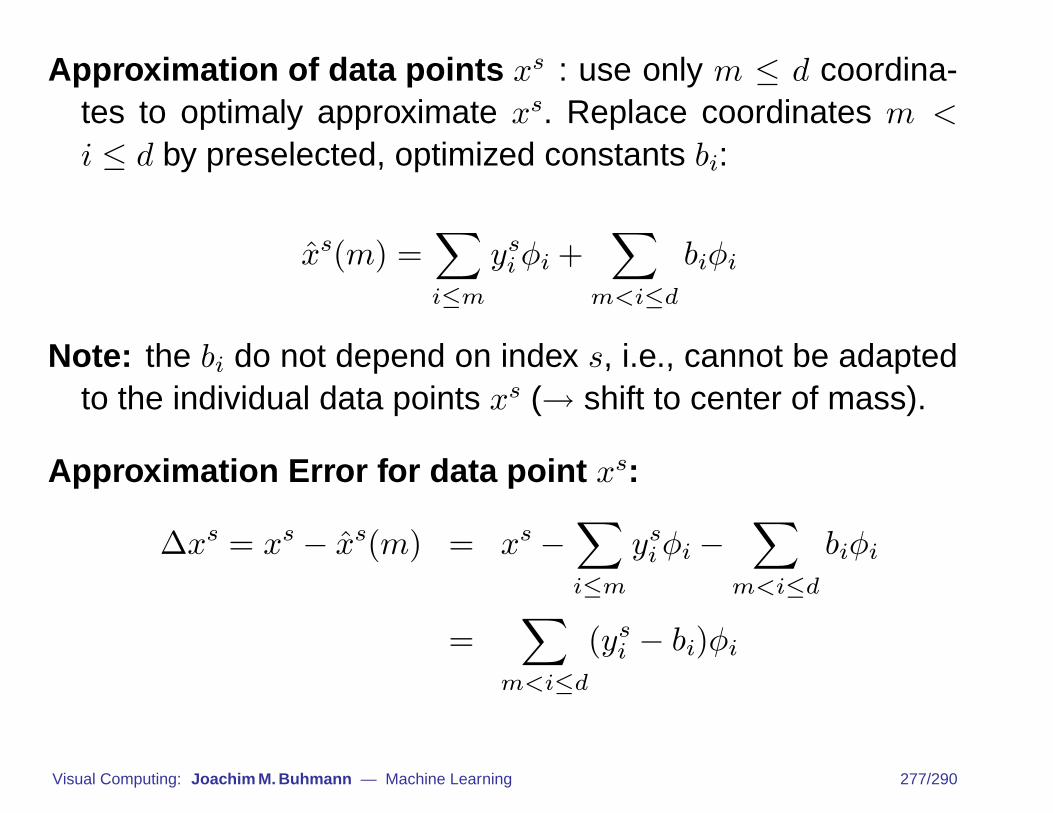
Approximation of data points xs : use only m ≤ d coordina-tes to optimaly approximate xs. Replace coordinates m <

i ≤ d by preselected, optimized constants bi:

x̂s(m) =∑i≤m

ysiφi +

∑m<i≤d

biφi

Note: the bi do not depend on index s, i.e., cannot be adaptedto the individual data points xs (→ shift to center of mass).

Approximation Error for data point xs:

∆xs = xs − x̂s(m) = xs −∑i≤m

ysiφi −

∑m<i≤d

biφi

=∑

m<i≤d

(ysi − bi)φi


A Quality-Measure of the Projection: Mean Squared Error

E{‖∆xs(m)‖2} =∑

m<i≤d

E{(ysi − bi)2}

“Interestingness” criterion in PCA: Choose the representa-tion with minimal E{‖∆xs(m)‖2}, i.e., optimize the bi, φi tominimize E{‖∆xs(m)‖2}.

Remark: An equivalent criterion is to maximize mutual infor-mation between original data points and their projections (as-sumption: Gaussian distribution of data).

Necessary condition for minimum:

∂

∂biE{(ys

i − bi)2} = −2(E{ys

i } − bi)

= 0

⇒ bi = E{ysi } = φ>i E{xs}


Inserting into the error criterion:

E{‖∆xs‖2} =∑

m<i≤d

E{(ys

i − E{ysi })2

}=

∑m<i≤d

φ>i E{(xs − E{xs})(xs − E{xs})>}︸︷︷︸=:ΣX

φi

Optimal Choice of Basis Vectors: Choose the eigenvectorsof the covariance matrix ΣX, i.e.,

ΣXφi = λiφi

Costs of PCA:

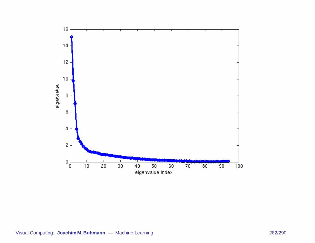
E{‖∆xs,opt(m)‖2} =∑

m<i≤d

λi


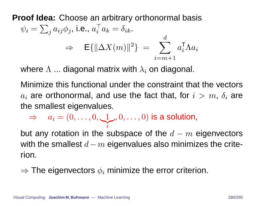
Proof Idea: Choose an arbitrary orthonormal basisψi =

∑j aijφj, i.e., a>i ak = δik.

⇒ E{‖∆X(m)‖2} =d∑

i=m+1

aTi Λai

where Λ ... diagonal matrix with λi on diagonal.

Minimize this functional under the constraint that the vectorsai are orthonormal, and use the fact that, for i > m, δi arethe smallest eigenvalues.⇒ ai = (0, . . . , 0, 1︸︷︷︸

i

, 0, . . . , 0) is a solution,

but any rotation in the subspace of the d − m eigenvectorswith the smallest d−m eigenvalues also minimizes the crite-rion.

⇒ The eigenvectors φi minimize the error criterion.


PCA: Summary

compute sample mean E{xs} and covariance matrix ΣX =E{(xs − E{xs′})(xs − E{xs′})>}

compute spectral decomposition ΣX = ΦΛΦ>

transformed data points: ys = Φ>(xs − E{xs′})

projection: for each ys, retain only those components i whereλi is among the largest m eigenvalues.


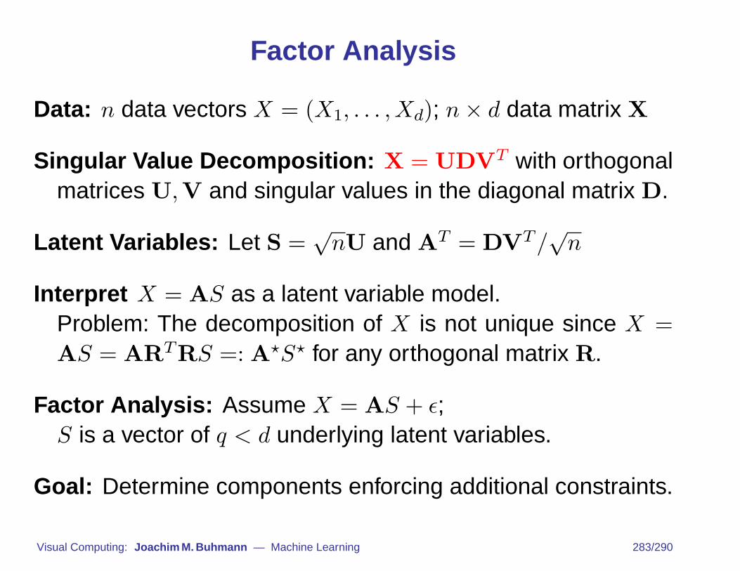
Factor Analysis

Data: n data vectors X = (X1, . . . , Xd); n× d data matrix X

Singular Value Decomposition: X = UDVT with orthogonalmatrices U,V and singular values in the diagonal matrix D.

Latent Variables: Let S =√nU and AT = DVT/

√n

Interpret X = AS as a latent variable model.Problem: The decomposition of X is not unique since X =AS = ARTRS =: A?S? for any orthogonal matrix R.

Factor Analysis: Assume X = AS + ε;S is a vector of q < d underlying latent variables.

Goal: Determine components enforcing additional constraints.


Independent Component Analysis

Find components which are statistically independent.

Measure of Dependence: Mutual Information

I(Y ) =∑j≤d

H(Yj)−H(Y ).

Strategy: find a decomposition X = AS which minimizesI(Y ) = I(ATX)

Procedure: perform a factor analysis and rotate the com-ponents to make them mutually independent.


Non-Linear Projection Methods

example: unfolding the locally linear, but globally highly nonli-near structure:

35. R. N. Shepard, Psychon. Bull. Rev. 1, 2 (1994).36. J. B. Tenenbaum, Adv. Neural Info. Proc. Syst. 10, 682

(1998).37. T. Martinetz, K. Schulten, Neural Netw. 7, 507 (1994).38. V. Kumar, A. Grama, A. Gupta, G. Karypis, Introduc-

tion to Parallel Computing: Design and Analysis ofAlgorithms (Benjamin/Cummings, Redwood City, CA,1994), pp. 257–297.

39. D. Beymer, T. Poggio, Science 272, 1905 (1996).40. Available at www.research.att.com/;yann/ocr/mnist.41. P. Y. Simard, Y. LeCun, J. Denker, Adv. Neural Info.

Proc. Syst. 5, 50 (1993).42. In order to evaluate the fits of PCA, MDS, and Isomap

on comparable grounds, we use the residual variance

1 – R2(D̂M , DY). DY is the matrix of Euclidean distanc-es in the low-dimensional embedding recovered byeach algorithm. D̂M is each algorithm’s best estimateof the intrinsic manifold distances: for Isomap, this isthe graph distance matrix DG; for PCA and MDS, it isthe Euclidean input-space distance matrix DX (exceptwith the handwritten “2”s, where MDS uses thetangent distance). R is the standard linear correlationcoefficient, taken over all entries of D̂M and DY.

43. In each sequence shown, the three intermediate im-ages are those closest to the points 1/4, 1/2, and 3/4of the way between the given endpoints. We can alsosynthesize an explicit mapping from input space X tothe low-dimensional embedding Y, or vice versa, us-

ing the coordinates of corresponding points {xi , yi} inboth spaces provided by Isomap together with stan-dard supervised learning techniques (39).

44. Supported by the Mitsubishi Electric Research Labo-ratories, the Schlumberger Foundation, the NSF(DBS-9021648), and the DARPA Human ID program.We thank Y. LeCun for making available the MNISTdatabase and S. Roweis and L. Saul for sharing relatedunpublished work. For many helpful discussions, wethank G. Carlsson, H. Farid, W. Freeman, T. Griffiths,R. Lehrer, S. Mahajan, D. Reich, W. Richards, J. M.Tenenbaum, Y. Weiss, and especially M. Bernstein.

10 August 2000; accepted 21 November 2000

Nonlinear DimensionalityReduction by

Locally Linear EmbeddingSam T. Roweis1 and Lawrence K. Saul2

Many areas of science depend on exploratory data analysis and visualization.The need to analyze large amounts of multivariate data raises the fundamentalproblem of dimensionality reduction: how to discover compact representationsof high-dimensional data. Here, we introduce locally linear embedding (LLE), anunsupervised learning algorithm that computes low-dimensional, neighbor-hood-preserving embeddings of high-dimensional inputs. Unlike clusteringmethods for local dimensionality reduction, LLE maps its inputs into a singleglobal coordinate system of lower dimensionality, and its optimizations do notinvolve local minima. By exploiting the local symmetries of linear reconstruc-tions, LLE is able to learn the global structure of nonlinear manifolds, such asthose generated by images of faces or documents of text.

How do we judge similarity? Our mentalrepresentations of the world are formed byprocessing large numbers of sensory in-puts—including, for example, the pixel in-tensities of images, the power spectra ofsounds, and the joint angles of articulatedbodies. While complex stimuli of this form canbe represented by points in a high-dimensionalvector space, they typically have a much morecompact description. Coherent structure in theworld leads to strong correlations between in-puts (such as between neighboring pixels inimages), generating observations that lie on orclose to a smooth low-dimensional manifold.To compare and classify such observations—ineffect, to reason about the world—dependscrucially on modeling the nonlinear geometryof these low-dimensional manifolds.

Scientists interested in exploratory analysisor visualization of multivariate data (1) face asimilar problem in dimensionality reduction.The problem, as illustrated in Fig. 1, involvesmapping high-dimensional inputs into a low-dimensional “description” space with as many

coordinates as observed modes of variability.Previous approaches to this problem, based onmultidimensional scaling (MDS) (2), havecomputed embeddings that attempt to preservepairwise distances [or generalized disparities(3)] between data points; these distances aremeasured along straight lines or, in more so-phisticated usages of MDS such as Isomap (4),

along shortest paths confined to the manifold ofobserved inputs. Here, we take a different ap-proach, called locally linear embedding (LLE),that eliminates the need to estimate pairwisedistances between widely separated data points.Unlike previous methods, LLE recovers globalnonlinear structure from locally linear fits.

The LLE algorithm, summarized in Fig.2, is based on simple geometric intuitions.Suppose the data consist of N real-valuedvectors WXi, each of dimensionality D, sam-pled from some underlying manifold. Pro-vided there is sufficient data (such that themanifold is well-sampled), we expect eachdata point and its neighbors to lie on orclose to a locally linear patch of the mani-fold. We characterize the local geometry ofthese patches by linear coefficients thatreconstruct each data point from its neigh-bors. Reconstruction errors are measuredby the cost function

ε~W ! 5 Oi

U WXi2SjWijWXjU

2

(1)

which adds up the squared distances betweenall the data points and their reconstructions. Theweights Wij summarize the contribution of thejth data point to the ith reconstruction. To com-pute the weights Wij, we minimize the cost

1Gatsby Computational Neuroscience Unit, Universi-ty College London, 17 Queen Square, London WC1N3AR, UK. 2AT&T Lab—Research, 180 Park Avenue,Florham Park, NJ 07932, USA.

E-mail: [email protected] (S.T.R.); [email protected] (L.K.S.)

Fig. 1. The problem of nonlinear dimensionality reduction, as illustrated (10) for three-dimensionaldata (B) sampled from a two-dimensional manifold (A). An unsupervised learning algorithm mustdiscover the global internal coordinates of the manifold without signals that explicitly indicate howthe data should be embedded in two dimensions. The color coding illustrates the neighborhood-preserving mapping discovered by LLE; black outlines in (B) and (C) show the neighborhood of asingle point. Unlike LLE, projections of the data by principal component analysis (PCA) (28) orclassical MDS (2) map faraway data points to nearby points in the plane, failing to identify theunderlying structure of the manifold. Note that mixture models for local dimensionality reduction(29), which cluster the data and perform PCA within each cluster, do not address the problemconsidered here: namely, how to map high-dimensional data into a single global coordinate systemof lower dimensionality.

R E P O R T S

www.sciencemag.org SCIENCE VOL 290 22 DECEMBER 2000 2323

What is the result of a linear projection?


Locally Linear Embedding (LLE)

Saul & Roweis: Nonlinear Dimensionality Reduction by Locally Linear Em-

bedding, Science 290, 2323(2000)

non-linear projection method

Basic Idea: use local patches

• each data point is related to a small number k of its neigh-bors

• relation within a patch is modeled in a linear way• k is the only free parameter


LLE Algorithm

1) compute neighbors of each data point xs, s = 1, ..., n.

2) approximate each data point xs ∈ Rp by x̂s =∑

tWstxt,where the xt’s are the neighbors of xs (linear approximation):find weights Wst that minimize

cost(W ) =∑

s

‖xs − x̂s‖2 =∑

s

‖xs −∑

t

Wstxt‖2

3) project to low-dimensional space: assume that weights Wst

capture local geometry also in low-dim. space. Given theweights Wst from 2), find projected points ys by minimizing

cost(y) =∑

s

‖ys −∑

t

Wstyt‖2 ys ∈ Rd, d� p


function subject to two constraints: first, thateach data point WXi is reconstructed only fromits neighbors (5), enforcing Wij 5 0 if WXj does

not belong to the set of neighbors of WXi;second, that the rows of the weight matrixsum to one: SjWij 5 1. The optimal weights

Wij subject to these constraints (6) are foundby solving a least-squares problem (7).

The constrained weights that minimizethese reconstruction errors obey an importantsymmetry: for any particular data point, theyare invariant to rotations, rescalings, andtranslations of that data point and its neigh-bors. By symmetry, it follows that the recon-struction weights characterize intrinsic geo-metric properties of each neighborhood, asopposed to properties that depend on a par-ticular frame of reference (8). Note that theinvariance to translations is specifically en-forced by the sum-to-one constraint on therows of the weight matrix.

Suppose the data lie on or near a smoothnonlinear manifold of lower dimensionality d,, D. To a good approximation then, thereexists a linear mapping—consisting of atranslation, rotation, and rescaling—thatmaps the high-dimensional coordinates ofeach neighborhood to global internal coordi-nates on the manifold. By design, the recon-struction weights Wij reflect intrinsic geomet-ric properties of the data that are invariant toexactly such transformations. We thereforeexpect their characterization of local geome-try in the original data space to be equallyvalid for local patches on the manifold. Inparticular, the same weights Wij that recon-struct the ith data point in D dimensionsshould also reconstruct its embedded mani-fold coordinates in d dimensions.

LLE constructs a neighborhood-preservingmapping based on the above idea. In the finalstep of the algorithm, each high-dimensionalobservation WXi is mapped to a low-dimensionalvector WYi representing global internal coordi-nates on the manifold. This is done by choosingd-dimensional coordinates WYi to minimize theembedding cost function

F~Y ! 5 Oi

U WYi 2 SjWijWYjU

2

(2)

This cost function, like the previous one, isbased on locally linear reconstruction errors,but here we fix the weights Wij while opti-mizing the coordinates WYi. The embeddingcost in Eq. 2 defines a quadratic form in thevectors WYi. Subject to constraints that makethe problem well-posed, it can be minimizedby solving a sparse N 3 N eigenvalue prob-lem (9), whose bottom d nonzero eigenvec-tors provide an ordered set of orthogonalcoordinates centered on the origin.

Implementation of the algorithm isstraightforward. In our experiments, datapoints were reconstructed from their K near-est neighbors, as measured by Euclidean dis-tance or normalized dot products. For suchimplementations of LLE, the algorithm hasonly one free parameter: the number ofneighbors, K. Once neighbors are chosen, theoptimal weights Wij and coordinates WYi are

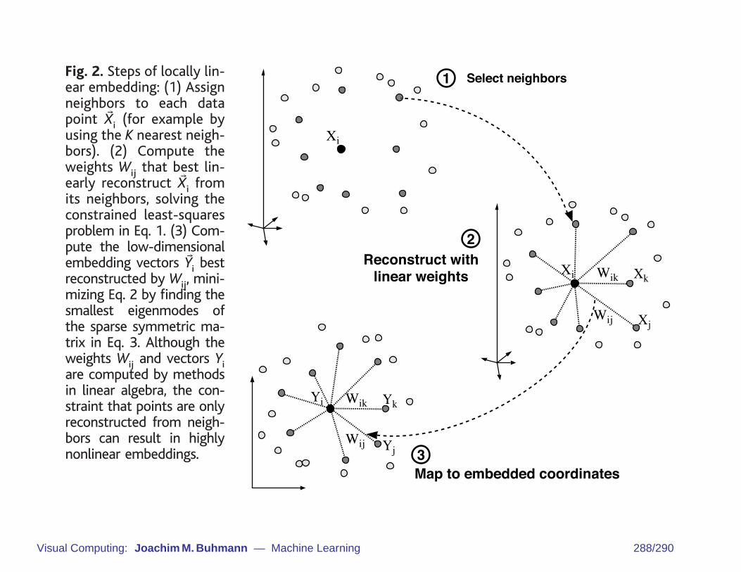
Fig. 2. Steps of locally lin-ear embedding: (1) Assignneighbors to each datapoint WXi (for example byusing the K nearest neigh-bors). (2) Compute theweights Wij that best lin-early reconstruct WXi fromits neighbors, solving theconstrained least-squaresproblem in Eq. 1. (3) Com-pute the low-dimensionalembedding vectors WYi bestreconstructed by Wij, mini-mizing Eq. 2 by finding thesmallest eigenmodes ofthe sparse symmetric ma-trix in Eq. 3. Although theweights Wij and vectors Yiare computed by methodsin linear algebra, the con-straint that points are onlyreconstructed from neigh-bors can result in highlynonlinear embeddings.

Fig. 3. Images of faces (11) mapped into the embedding space described by the first twocoordinates of LLE. Representative faces are shown next to circled points in different parts of thespace. The bottom images correspond to points along the top-right path (linked by solid line),illustrating one particular mode of variability in pose and expression.

R E P O R T S

22 DECEMBER 2000 VOL 290 SCIENCE www.sciencemag.org2324


Remarks on LLE

constraints on weights:

• Wst = 0 unless xs and xt are neighbors.• normalization: for all s:

∑tWst = 1.

Reason for constraints: this ensures invariance to rotation,rescaling, translation of data points.

Optimization:

• step 2): solve least squares problem• step 3): solve n× n eigenvector problem• no local minima• computational complexity is quadratic in n


function subject to two constraints: first, thateach data point WXi is reconstructed only fromits neighbors (5), enforcing Wij 5 0 if WXj does

not belong to the set of neighbors of WXi;second, that the rows of the weight matrixsum to one: SjWij 5 1. The optimal weights

Wij subject to these constraints (6) are foundby solving a least-squares problem (7).

The constrained weights that minimizethese reconstruction errors obey an importantsymmetry: for any particular data point, theyare invariant to rotations, rescalings, andtranslations of that data point and its neigh-bors. By symmetry, it follows that the recon-struction weights characterize intrinsic geo-metric properties of each neighborhood, asopposed to properties that depend on a par-ticular frame of reference (8). Note that theinvariance to translations is specifically en-forced by the sum-to-one constraint on therows of the weight matrix.

Suppose the data lie on or near a smoothnonlinear manifold of lower dimensionality d,, D. To a good approximation then, thereexists a linear mapping—consisting of atranslation, rotation, and rescaling—thatmaps the high-dimensional coordinates ofeach neighborhood to global internal coordi-nates on the manifold. By design, the recon-struction weights Wij reflect intrinsic geomet-ric properties of the data that are invariant toexactly such transformations. We thereforeexpect their characterization of local geome-try in the original data space to be equallyvalid for local patches on the manifold. Inparticular, the same weights Wij that recon-struct the ith data point in D dimensionsshould also reconstruct its embedded mani-fold coordinates in d dimensions.

LLE constructs a neighborhood-preservingmapping based on the above idea. In the finalstep of the algorithm, each high-dimensionalobservation WXi is mapped to a low-dimensionalvector WYi representing global internal coordi-nates on the manifold. This is done by choosingd-dimensional coordinates WYi to minimize theembedding cost function

F~Y ! 5 Oi

U WYi 2 SjWijWYjU

2

(2)

This cost function, like the previous one, isbased on locally linear reconstruction errors,but here we fix the weights Wij while opti-mizing the coordinates WYi. The embeddingcost in Eq. 2 defines a quadratic form in thevectors WYi. Subject to constraints that makethe problem well-posed, it can be minimizedby solving a sparse N 3 N eigenvalue prob-lem (9), whose bottom d nonzero eigenvec-tors provide an ordered set of orthogonalcoordinates centered on the origin.

Implementation of the algorithm isstraightforward. In our experiments, datapoints were reconstructed from their K near-est neighbors, as measured by Euclidean dis-tance or normalized dot products. For suchimplementations of LLE, the algorithm hasonly one free parameter: the number ofneighbors, K. Once neighbors are chosen, theoptimal weights Wij and coordinates WYi are

Fig. 2. Steps of locally lin-ear embedding: (1) Assignneighbors to each datapoint WXi (for example byusing the K nearest neigh-bors). (2) Compute theweights Wij that best lin-early reconstruct WXi fromits neighbors, solving theconstrained least-squaresproblem in Eq. 1. (3) Com-pute the low-dimensionalembedding vectors WYi bestreconstructed by Wij, mini-mizing Eq. 2 by finding thesmallest eigenmodes ofthe sparse symmetric ma-trix in Eq. 3. Although theweights Wij and vectors Yiare computed by methodsin linear algebra, the con-straint that points are onlyreconstructed from neigh-bors can result in highlynonlinear embeddings.

Fig. 3. Images of faces (11) mapped into the embedding space described by the first twocoordinates of LLE. Representative faces are shown next to circled points in different parts of thespace. The bottom images correspond to points along the top-right path (linked by solid line),illustrating one particular mode of variability in pose and expression.

R E P O R T S

22 DECEMBER 2000 VOL 290 SCIENCE www.sciencemag.org2324Visual Computing: Joachim M. Buhmann — Machine Learning 290/290

machine learning: topic chart - ethz - home · pdf filemachine learning: topic chart ......

Documents