machine learning to balance the load in parallel branch ... · learning · unit commitment ......
TRANSCRIPT

Noname manuscript No.(will be inserted by the editor)
Machine Learning to Balance the Load in Parallel
Branch-and-Bound
Alejandro Marcos Alvarez · LouisWehenkel · Quentin Louveaux
Received: date / Accepted: date
Abstract We describe in this paper a new approach to parallelize branch-and-bound on a certain number of processors. We propose to split the opti-mization of the original problem into the optimization of several subproblemsthat can be optimized separately with the goal that the amount of work thateach processor carries out is balanced between the processors, while achiev-ing interesting speedups. The main innovation of our approach consists in theuse of machine learning to create a function able to estimate the difficulty(number of nodes) of a subproblem of the original problem. We also presenta set of features that we developed in order to characterize the encounteredsubproblems. These features are used as input of the function learned withmachine learning in order to estimate the difficulty of a subproblem. The es-timates of the numbers of nodes are then used to decide how to partition theoriginal optimization tree into a given number of subproblems, and to decidehow to distribute them among the available processors. The experiments thatwe carry out show that our approach succeeds in balancing the amount ofwork between the processors, and that interesting speedups can be achievedwith little effort.
Keywords Parallel branch-and-bound · Hardness estimation · Machinelearning · Unit commitment
Mathematics Subject Classification (2010) 90C57 · 90C27 · 68T20
A. Marcos Alvarez, L. Wehenkel, Q. LouveauxDepartment of Electrical Engineering and Computer ScienceUniversite de LiegeLiege, BelgiumE-mail: {amarcos,l.wehenkel,q.louveaux}@ulg.ac.be

2 Marcos Alvarez, Wehenkel, Louveaux
1 Introduction
Branch-and-bound (B&B), and its variants, is probably the most popular algo-rithm used to solve mixed-integer programming (MIP) problems. Throughoutthe years, its internal mechanisms were improved and many additional fea-tures such as cutting planes, advanced branching strategies and presolve havebeen added to the core algorithm. These many improvements made it easy tosolve problems of ever increasing size. However, since B&B is mainly devotedto solving NP-hard problems, some of them remain nowadays still too difficultto be solved by a single sequential B&B.
Parallelizing B&B on a large number of computers is a promising way tosolve those problems that remain out of reach of traditional approaches. Thisrationale is strongly motivated by two arguments. First, B&B is a naturalcandidate for parallelization since it relies on the divide-and-conquer paradigm.Parallelizing B&B is indeed conceptually quite simple, and mainly consists individing the original optimization tree in several subtrees, or subproblems,and let each processor, or worker, work on its own part of the global tree. Twoparallel implementations mainly differ in the way the original work is splitamong the available workers, and by the amount of communication involvedin the optimization. The second argument in favor of parallel B&B is theexplosion of parallel computing and affordable massively parallel computersthat has been witnessed in the last two to three decades.
Based on these observations, many researchers started developing parallelB&B algorithms. One of the first reported attempts to parallelize B&B datesback to 1975 and is summarized in a 1988 paper by Pruul et al (1988). In thatpaper, Pruul et al describe a simple approach to parallelize B&B on a sharedmemory serial computer. They report a set of experimental results obtained onthe travelling salesman problem and analyze the efficiency of their approach.One important finding is that the number of explored nodes might be less inthe parallel case than in the serial case. As a consequence, the achieved speedupcomputed from the number of explored nodes might be higher than the numberof processors on which the B&B has been parallelized. These findings furthersupport the idea that parallel B&B is a front-running candidate to solve largeMIP problems. It has to be noted however that there exist special cases wherethe parallel version of B&B performs worse than its serial counterpart (see,e.g., Lai and Sahni 1984).
Very early, balancing the load of each worker of a parallel B&B has be-come a major concern. Indeed, as for any parallel algorithm, load balance isa crucial aspect that must addressed in order to achieve interesting speedups.Throughout the years, several load balancing schemes have been proposed.For instance, El-Dessouki and Huen (1980) propose a mixed static and dy-namic balancing scheme that gives each processor the responsibility to com-pute its own subtree, and allows them to help other processors when theirown workload has been exhausted. Later, Karp and Zhang (1988) proposed afully dynamic work distribution method that automatically balances the loadof each worker by sending the newly created children to random processors.

Machine Learning to Balance the Load in Parallel Branch-and-Bound 3
Rao and Kumar (1987) also proposed several load balancing schemes tailoredto different parallel architectures (see also Kumar and Rao 1987).
A common shortcoming of all the dynamic load balancing schemes is thatthey imply a large amount of communications. It became very early clear thatthe overhead cost induced by communication times was a major concern forall parallel B&B implementations. On the one hand, communication is desir-able because it allows to better balance each processor’s load by ensuring thatno processor remains idle while others are working. Moreover, communica-tion can also reduce the total amount of work to be done by all processors bysharing information about feasible solutions. But, despite its advantages, com-munication between processors remains very expensive and should be limitedto its minimum. Laursen (1994) was one of the first to propose a method inwhich the processors do not communicate with each other and that allocatesstatically the workload to each worker. Of course, the key factor of successof this approach is to evaluate accurately enough the difficulty of the sub-tree given to each processor. If the workload is not well balanced between theworkers, the utilization of the processors will not be optimal. One of the ap-proaches proposed by Laursen consists in finding a function that predicts thenumber of nodes of a subtree, i.e., its difficulty, from a set of characteristicsextracted from the subtree. Laursen carried out a series of experiments withseveral functions constructed from simple functional forms like the exponen-tial or the logarithm. Unfortunately, each considered function was not able toconsistently predict the difficulty of several classes of problems. Laursen con-cluded that it was not trivial to find such a function. Later, the idea proposedby Laursen (1994) has been further explored in a more principled approachby Otten and Dechter (2012) who used machine learning techniques to createa function that can be used to predict the difficulty of a subproblem basedon easily computable features. They reported good results for a given classof MIP problems represented over graphical models solved by an AND/ORbranch-and-bound.
In a slightly different fashion, Wah and Yu (1985) and Yang and Das (1994)have developed interesting approaches to evaluate the difficulty of a subprob-lem. Both approaches are based on probabilistic models that are used to pre-dict the complexity of a subproblem. Despite the encouraging results that theyreport, the assumptions required by the probabilistic models seem very strongand unrealistic for a wide variety of problems.
The interest in parallel B&B is not limited to the field of optimization.Indeed, parallelizing B&B has also attracted some attention in the computerscience community that developed several frameworks aimed at easing the im-plementation of personal specialized parallel B&B algorithms (see, e.g., Eck-stein et al 2001; Dorta et al 2004). It must be noted that the pieces of workreported in this paper are by no means exhaustive, and we refer the readerto Gendron and Crainic (1994)’s paper for a wider, though older, survey ofparallel B&B techniques.
Based on the previously made observations and on previous work, andfurther supported by the conclusions drawn by Linderoth (1998, p. 197), we

4 Marcos Alvarez, Wehenkel, Louveaux
propose in this paper a new approach using machine learning to balance theload between several processors, and apply our approach to a set of unit com-mitment (UC) problems. The main contribution of this work is the develop-ment of an approach using machine learning to create and distribute severalsubproblems to a given number of processors such that the workloads of eachprocessor are not too dissimilar. Moreover, we develop a set of new featuresthat allow to represent a subproblem in order to predict its difficulty, in termsof the number of nodes. The experimental results show that the approach suc-ceeds in efficiently balancing the load between several processors, and that itachieves interesting results with and without communication. It is to be notedthat the developed features do not depend on the class of problems used toassess our method. They are virtually applicable to any type of MIP problem,although some adaptation might be necessary to improve the performance ona given class of problems. Moreover, we must emphasize that machine learn-ing is mainly useful when the considered problems are related to each other,otherwise it is in general difficult for the algorithm to learn something fromthe available data. Because of these requirements, the proposed approach isprimarily applicable to the situations where similar problems have to be re-peatedly solved over time. Focusing on unit commitment (UC) problems isthus a straightforward choice since generation companies, or transmission sys-tem operators, have to repeatedly solve very similar UC problems again andagain.
In the remainder of the paper, we start first, in Section 2, by giving somepreliminary information about the considered problem and by introducingimportant concepts. We then describe the method that we propose in Section 3.A short theoretical analysis is next carried out in Section 4. Section 5 thendescribes a series of experiments that we perform in order to validate ourapproach. Finally, Section 6 concludes this paper and draws some lines offuture work.
2 Preliminaries
We first describe here in a more detailed way the problem addressed in thispaper, and give a brief introduction to machine learning for the beginner.
2.1 Problem statement
In this paper, we want to develop an efficient parallel version of a branch-and-bound algorithm that minimizes the amount of communication and thatachieves high speedups. To do so, we will split the original optimization treeinto several subtrees that cover together the initial tree. Each subtree is thengiven to a processor (a processor can be responsible for several subtrees) thatis asked to solve the subproblem defined by each subtree. Communication be-tween processors is ideally forbidden, but a small amount can still be allowed in

Machine Learning to Balance the Load in Parallel Branch-and-Bound 5
order to benefit from the solutions found by other processors. Because commu-nication should be maintained at its minimum, the workload of each processor,i.e., the difficulty of the given set of subtrees, should ideally be balanced be-tween all processors so that high speedups can be achieved. Balancing theworkload is the problem tackled in this paper.
In the context of optimization, the workload is basically the time a solverneeds to find the optimal solution, but other difficulty measures are also com-monly used. For instance, in the case of B&B, it is acknowledged that thenumber of nodes explored by the algorithm before optimality is proved favor-ably estimates the difficulty of a problem. In this paper, we focus on the latterdifficulty measure, i.e., the number of nodes, as it is more robust to pertur-bations during the experiments, and roughly linearly dependent (up to a timefactor) on the optimization time. Consequently, the focus of this paper is todevelop a method that balances the numbers of nodes of the subtrees thateach processor is responsible for.
In this work, we address binaryMixed-Integer Linear Programming (MILP)problems of the form
min c⊤x (1)
s.t. Ax ≤ b
xj ∈ {0, 1} ∀j ∈ I
xj ∈ R+ ∀j ∈ C,
where c ∈ Rn, A ∈ R
m×n and b ∈ Rm respectively denote the cost coefficients,
the coefficient matrix and the right-hand side. I and C are two sets containingthe indices of the integer and continuous variables respectively. We denote thesolution at a given node of the B&B by x∗ and we will call, with a little abuse,the variable xi, with i ∈ I, a fractional variable if it has a fractional value inthe current solution x∗.
2.2 Introduction to machine learning
Machine learning (ML) is the field of artificial intelligence that is concerned bythe automatic construction, or learning, of functions from data. Let us assumewe are interested in some task T that maps states s belonging to S, which isthe set of possible input states of the task, to an output space Y. Basically,ML focuses on the construction of functions f imitating the behavior of T .More specifically, the functions f map inputs from a space Φ to the outputspace Y, i.e., f (·) ∈ F : Φ 7→ Y, where F is the set of possible mappings fromΦ to Y. Formally, a machine learning algorithm A is a procedure of the form
A : (Φ× Y)N 7→ F
that takes as input a dataset D = ((φi, yi))N
i=1 ∈ (Φ× Y)N , and that outputsa function f ∈ F that minimizes some loss function L on the dataset D.

6 Marcos Alvarez, Wehenkel, Louveaux
Stated in mathematical terms, the function f∗ resulting from the applicationof algorithm A to dataset D is given by
f∗ = A (D) = argminf∈F
N∑
i=1
L (yi, f (φi)) .
Note that the set F of possible output functions depends on the particularclass of machine learning algorithm that is used.
Ideally, the input of function f should be s ∈ S, the input state of T itself.However, representing the complete state is often a difficult problem, e.g.,because its dimensionality is too big, or because it contains a lot of irrelevantinformation. For this reason, in the machine learning community, the inputsφ of the functions f are usually ‘features’ representing a simplified version ofthe input state. Formally, features are (vectors of) characteristics extractedheuristically from the input state s ∈ S, i.e.,
C (s) = φ ∈ Φ ⊂ Rd,
such that those features represent part of the current state, ideally the partthat most influences the output. The features often critically condition theefficiency of learning methods. As they represent only part of the currentstate of the task, it is important that the parts described by the features areindeed correlated to the desired output. For this reason, the features need tobe carefully designed and tailored to the problem of interest.
The strength of machine learning relies on its ability to generalize behav-iors observed on data with very few assumptions needed. This makes it apowerful tool when one wants to imitate unknown functions for which no, orvery little, information is available. The main requirement is that the machinelearning procedure needs a dataset containing pairs of inputs and outputs(φi, yi) obtained from the task T that the ML algorithm is trying to imitate.Those input-output pairs can be obtained by simulation or through a black-box function, there is no need to actually know the functional representationof the real underlying function to be learned.
3 Description of the method
In this section, we describe the method that we devised in order to balance theload of each individual processor of a parallel branch-and-bound. We first de-scribe how we generate a set of subproblems that span the entire optimizationtree. We next describe how the subproblems can be allocated to the differentprocessors.
3.1 Generating a partition of the original optimization tree
The approach that we propose to generate a partition of the optimizationtree is very much alike a traditional branch-and-bound. It is represented inAlgorithm 1.

Machine Learning to Balance the Load in Parallel Branch-and-Bound 7
In this algorithm, we generate a partition of the original optimization treecontaining at most k elements. From now on, the notation p represents asubproblem of the original problem, i.e., a problem for which a certain numberof binary variables are fixed either to 0 or 1. In particular, p0 designates theroot node, i.e., a version of the original problem in which no binary variable isfixed. The algorithm first starts with p0 that is added to a queue. Then, theprocedure is as follows. The algorithm retrieves and removes a subproblem pfrom the queue and iteratively creates a certain number of children of p bysetting each unfixed binary variable in p to 0 and then to 1. Thus, for eachunfixed binary variable, we create two children by fixing that variable eitherto 0 or to 1. A set of features describing each child created in that way is thencomputed with a given function C. The computed features are subsequentlyused as input of a learned complexity function fnodes that returns an estimateof the number of nodes required to solve the child subproblem represented bythe features. The predictions of the numbers of nodes of each child are nextused to compute a score according to which the unfixed binary variables in thesubproblem p are ranked. Once every unfixed binary variable has been scored,the two child subproblems corresponding to the variable that has the lowestscore are added to the queue. The presented procedure is then repeated byremoving from the queue the subproblem whose predicted number of nodesis the greatest, until the queue fulfills a given stopping criterion or until amaximum queue size has been reached.
In the end of the procedure, each element of the queue represents the rootnode of a subtree forming the sought partition of the original optimizationtree.
The behavior of the proposed partitioning algorithm depends on three mainfactors: the function fnodes predicting the number of nodes of a subproblem;the way the features are computed, i.e., the implementation of function C (·);and the implementation of the function score (·). The rest of this section detailshow these functions were implemented in this work.
3.1.1 Assessing the difficulty of a subproblem
In order to create a partition of the original optimization tree that balanceswell the workload of each processor, our procedure requires that a functionable to predict the difficulty of a subproblem is available. As previous researchindicates (Wah and Yu 1985; Yang and Das 1994; Laursen 1994), it is nottrivial to find a simple mathematical formulation for such a function. We thusdecided to resort to machine learning in order to create that function.
There exist several machine learning frameworks that could be used to con-struct a function. In this work, we apply the supervised learning framework.In this approach, a dataset containing input-output pairs is needed by the ma-chine learning algorithm to construct the desired function. The input-outputpairs should be observations of the system that the function is supposed toimitate. In this work, the inputs consist in feature vectors, i.e., vectors ofscalars, that represent some characteristics of the subproblem. The output of

8 Marcos Alvarez, Wehenkel, Louveaux
Algorithm 1 Optimization tree partitioning algorithm1: q = p0 ⊲ p0 is the root node2: while true do
3: if |q| ≥ k then ⊲ k is the maximum number of elements in the partition4: break
5: else if |q| ≥ 3N then ⊲ N is the number of available processors6: if maxp∈q fnodes (C (p)) ≤ 3
4N
∑
p∈q fnodes (C (p)) then
7: break
8: end if
9: end if
10: p = argmaxp′∈q fnodes (C (p′))11: s∗ = +∞12: for i ∈ Up do ⊲ Up is the set of indices of the unfixed binary variables in p13: pleft = p with xi set to 014: nleft = fnodes (C (pleft)) ⊲ C is the function that generates the features15: pright = p with xi set to 116: nright = fnodes
(
C(
pright))
⊲ n is an estimate of the number of nodes of p17: s = score(nleft, nright)18: if s < s∗ then
19: s∗ = s20: p∗
left= pleft
21: p∗right
= pright22: end if
23: end for
24: q = q \ p ∪{
p∗left
, p∗right
}
25: end while
26: return q
the function is the number of nodes the subproblem requires in order to besolved. The output thus gives an idea of how difficult a subproblem is.
More specifically, the function that we learn is
fnodes : Φ ⊂ Rd 7→ R,
where Φ is the set of possible feature vectors that is included in Rd. In principle,
the output should be an integer, but this is not guaranteed by the machinelearning algorithm. We thus allow the estimated number of nodes to be ageneral scalar instead of an integer.
The supervised learning framework requires that a dataset of input-outputpairs observed from the system we are trying to imitate is available for learning.In our case, such a dataset is not available and we must thus create one so thatour method can be applied. In order to do that, we first select a set of problems.We next randomly generate, for each problem in this set, a certain numberof subproblems by randomly fixing each variable in a subset of the binaryvariables to 0 or 1. For instance, if the problem contains 20 binary variables,we will select a random subset of them, and randomly fix each variable in thissubset to 0 or 1. The created subproblem is then optimized until optimalityis reached. This gives the number of nodes, and, hence, the difficulty of thesubproblem that will be the output part of a pair of the dataset. The inputpart is given by the feature vector that will be computed for the randomly

Machine Learning to Balance the Load in Parallel Branch-and-Bound 9
generated subproblem. This procedure is repeated until enough data has beengenerated.
Once the dataset is created, we can apply a supervised machine learningalgorithm in order to learn the function fnodes from the observed data. In thiswork, we used the random forests algorithm (Breiman 2001).
3.1.2 Computing the features of a subproblem
As mentioned in the previous section, the input of the function fnodes shouldbe a vector of scalars. This section describes how these features are computedfor a given subproblem.
A subproblem p is created by fixing a certain amount of binary variableseither to 0 or to 1. We denote by Fp the set of the indices of the fixed binaryvariables, and the set of unfixed binary variables by Up. The indices of thevariables fixed to 0 and 1 are respectively contained in the sets Fp0 and Fp1.Note that we assume that all problems are in the form (1) and that we willuse the same notations.
We denote the LP solution of the root node of the original problem by x∗0,
and the solution at the root of the subproblem p by x∗p. Similarly, the value of
the objective function obtained with the solutions x∗0 and x∗
p are denoted o∗0and o∗p, respectively. We moreover assume that a heuristic solution is availablefrom the beginning. The heuristic function h(·) applied to solution x∗
0 gives thesolution xh
0 = h(x∗0), and the value of the objective function for this solution
is oh0 . This heuristic solution allows us to compute the initial gap gi at the rootnode of subproblem p, that is,
gi =oh0 − o∗p
oh0.
Note that this gap can be negative since the LP objective of the subproblemcan be greater than the objective of the heuristic solution computed at theroot node of the original problem.
Additionally, we compute, for each subproblem p, a new right hand side bi,for each constraint i. Indeed, since some variables are fixed in p, the values oftheir coefficients in the constraint matrix A, multiplied by their value, can besubtracted from the initial b. We thus define the new right hand side as
bi = bi −∑
j∈Fp1
Aij ,
since it is not necessary to subtract the coefficients of the variables fixed to 0.In order to compute additional features, we also optimize, for a very short
period of time, the subproblem p with a traditional B&B. More specifically,we allow 5,000 nodes to be explored. Note that the algorithm uses as primalbound the value of the objective function found by the heuristic at the rootnode, i.e., oh0 . When this budget is exhausted, we extract a certain number ofcharacteristics from the optimization. This phase is called probing. At the end

10 Marcos Alvarez, Wehenkel, Louveaux
of the optimization budget, we retrieve the dual bound oprobingdual and the new
primal bound oprobingprimal . With these values, we can compute the final gap gf atthe end of the probing with
gf =oprobingprimal − oprobingdual
oprobingprimal
.
Besides the previous values that must be recomputed for each new sub-problem p, we carry out some preliminary calculations whose results will besubsequently used to extract characteristics of any subproblem p. More specif-ically, we compute the relative objective increase observed between the rootnode of the original problem and the subproblem created by fixing a specificbinary variable xj , with j ∈ I, to 0 or 1. We thus obtain two vectors oi0 andoi1, such that
oi0(j) =o∗pxj=0
− o∗0
|o∗0|and oi1(j) =
o∗pxj=1− o∗0
|o∗0|,
where pxj=0 (respectively pxj=1) is the subproblem created by fixing variablexj to 0 (respectively 1), and leaving all other variables unfixed. These vectorsare computed once and for all in the beginning, and will be used to computesome of our features.
The above description merely introduces some notations and some valuesused to compute our features describing a subproblem. The complete list thatwe use in this work is given in Table 1. In this table, the features are separatedinto five categories, each one of which is meant to represent different dynamicsof the problem. The first category of features captures basic characteristicsof the subproblem, as well as some differences between the subproblem andthe original root problem, like the increase of the LP objective between theroots of both problems. The second category aims at representing the differentinteractions that exist between the fixed binary variables of the subproblemand the other binary variables in the cost function and in the constraints.Then, the features in the third category model the sparsity of the subprob-lem with different measures computed from the subproblem and the originalproblem. The fourth category is similar to the second one except that its goalis to evaluate the connections between all variables (fixed, unfixed binary andcontinuous variables) in the objective function as well as in the constraints.Finally, the fifth category contains the features that are computed after theprobing phase. These features give a small glimpse of the optimization of thesubproblem.
3.1.3 Scoring a variable
In the algorithm that we propose, a score is used to determine which variableit is better to branch on in order to expand the current tree by two newlycreated nodes. The way the score is computed influences the behavior of the

Machine Learning to Balance the Load in Parallel Branch-and-Bound 11
Table 1 Features used to describe a subproblem
Feat. # Description
1∣
∣o∗0 − o∗p∣
∣ /∣
∣o∗0∣
∣
2-3 |Fp0|/|I| and |Fp1|/|I|
4 |Up|/|I|
5(
∑
j∈Fp0|0− x∗
0(j)|+∑
j∈Fp1|1− x∗
0(j)|)
/|Fp|
6-9 minj∈Fp0oi0(j), plus the max, mean and std of those values
10-13 minj∈Fp1oi1(j), plus the max, mean and std of those values
14-17 minj∈Up0.5 ∗ oi0(j) + 0.5 ∗ oi1(j), plus the max, mean and std of those
values
18(
oh0 − o∗p)
/|oh0 |
19∑
j∈Fpcj/
∑
j∈I cj
20∑
j∈Upcj/
∑
j∈I cj
21-22 mini=1...m
(
bi −∑
j∈Fp1Aij
)
/bi, plus the max of those values
23-24 mini=1...m
∑
j∈UpAij/bi, plus the max of those values
25-26 mini=1...m
(
∑
j∈UpAij − bi
)
/bi, plus the max of those values
27-28 mini=1...m
∑
j∈FpAij/
∑
j∈I Aij , plus the max of those values
29-30 mini=1...m
∑
j∈UpAij/
∑
j∈I Aij , plus the max of those values
31-34 meanj∈Fp‖A:j‖0 /m, plus the min, max, and std of those values
35-38 meanj∈Up‖A:j‖0 /m, plus the min, max, and std of those values
39-42 meanj∈C ‖A:j‖0 /m, plus the min, max, and std of those values
43∑
j∈Fpcj/
∑nj=1 cj
44∑
j∈Upcj/
∑nj=1 cj
45∑
j∈C cj/∑n
j=1 cj
46-47 mini=1...m
∑
j∈FpAij/
∑nj=1 Aij , plus the max of those values
48-49 mini=1...m
∑
j∈UpAij/
∑nj=1 Aij , plus the max of those values
50-51 mini=1...m
∑
j∈C Aij/∑n
j=1 Aij , plus the max of those values
52-53 mini:bi≥0
(
∑
j∈Up:Aij≥0 Aij +∑
j∈C:Aij≥0 Aij
)
/bi, plus the max of
those values
54-55 mini:bi≥0
(
∑
j∈Up:Aij<0 Aij +∑
j∈C:Aij<0 Aij
)
/bi, plus the max of
those values
56-57 mini:bi<0
(
∑
j∈Up:Aij≥0 Aij +∑
j∈C:Aij≥0 Aij
)
/bi, plus the max of
those values
58-59 mini:bi<0
(
∑
j∈Up:Aij<0 Aij +∑
j∈C:Aij<0 Aij
)
/bi, plus the max of
those values
60(
oprobingdual
− o∗p
)
/oprobingdual
61(
oh0 − oprobingprimal
)
/oh0
62 ratio between the number of open nodes left after the probing budget isexhausted and the number of explored nodes
63 maximum depth of the probing tree
64 depth of the last full level (i.e., the level l such that the numbers of nodes
in the levels l′ = 1 . . . l are 2l′
) in the probing tree
65 waist of the probing tree (i.e., level l with the largest number of nodes)
66 100 ∗ (gi − gf )/|gi|

12 Marcos Alvarez, Wehenkel, Louveaux
tree partitioning algorithm. The first score that we propose aims at balancingthe difficulty, i.e., the number of nodes, of each newly created children. Theproposed score is as follows:
score(nleft, nright) =nleft + nright
2+
∣
∣
∣
∣
nright − nleft
2
∣
∣
∣
∣
+
∣
∣
∣
∣
nleft − nright
2
∣
∣
∣
∣
,
where nleft and nright respectively indicate the predicted size of the left andright subproblems.
The other proposed scoring criterion is designed such that the total amountof work is minimized. It is given by
score(nleft, nright) = max (nleft, nright) .
This score does not take into account the difficulty equilibrium between thetwo created nodes. It is assumed that the balance can be achieved later whenthe generated subproblems are distributed to the workers.
3.2 Distributing nodes to processors
In the case where the number k of generated subproblems is equal to thenumber of processors, the distribution of the work is trivial. If the numberof nodes in the partition is greater than the number of processors, one mustfind a way to distribute the work evenly between the processors such that theworkload is well balanced between each worker.
There exist several ways this distribution could be done. In this work, weapplied a simple greedy method although other, more formal, approaches areapplicable. The greedy routine that we use is detailed in Algorithm 2. Theoutput of this algorithm is an array, one element per processor, of queuesspecifying which subproblems have to be solved by a given processor.
Algorithm 2 Greedy subproblem allocation1: let N be the number of processors2: let h be an array of N scalars3: let q be an array of N queues4: let l be a list containing the subproblems of the tree partition5: h(i) = 0, ∀i6: q(i) = ∅, ∀i7: while l 6= ∅ do
8: p = argmaxp′∈l fnodes(p′) ⊲ select the most difficult remaining subproblem
9: k = argmini=1...N h(i) ⊲ identify the queue whose expected workload is the least10: h(k) = h(k) + fnodes(p)11: q(k) = q(k) ∪ p ⊲ add the current subproblem to the chosen queue12: l = l \ p13: end while
14: return q

Machine Learning to Balance the Load in Parallel Branch-and-Bound 13
A more formal approach to allocate the subproblems to the workers is tosolve the following problem:
min
N∑
i=1
zi (2)
s.t.
k∑
j=1
aij nj = wi ∀i = 1 . . .N
N∑
i=1
aij = 1 ∀j = 1 . . . k
m− wi ≤ zi, m− wi ≥ −zi ∀i = 1 . . .N
aij ∈ {0, 1} , wi, zi ∈ R+,
where k and N respectively correspond to the number of subproblems to beallocated and to the number of processors, and nj andm respectively representthe predicted number of nodes of a subproblem and the ideal average load of
each processor, i.e.,∑
jnj
N.
4 Theoretical analysis
In this section, we present a short theoretical analysis that can be derived fromour method. Indeed, one of the side advantages of using machine learning isthat it is possible to get in advance, i.e., without performing the optimization,an estimate of the number of nodes that a subproblem needs in order to besolved to optimality. Moreover, the error of this estimate can be estimatedas well. In the following, we show how these estimates can be used to get anapproximation of the speedup of the method before the optimization is carriedout.
In general, it is easier to reach an equilibrium between the workloads of eachprocessor when the chunks that have to be distributed are smaller. For thisreason, it might be better to generate a number of subproblems that is greaterthan the number of processors. Each worker j thus has a queue qj containingthe subproblems for which it is responsible. Thanks to machine learning, thenumber of nodes ni that a subproblem pi requires can be estimated with thelearned function, i.e., ni = fnodes(pi). In practice however, the prediction isnot perfect, and we can assume that the real number of nodes ni required tosolve the subproblem to optimality is a random variable that is distributedaround the predicted value ni.
Assuming that the mean of ni is ni and that its standard deviation is σi, thefollowing theorems characterize a given subproblem allocation. We propose twotheorems that characterize, respectively, the speedup obtained with a parallelwork distribution, and its absolute duration, i.e., the maximum number ofnodes over all processors. Both theorems provide information that can be

14 Marcos Alvarez, Wehenkel, Louveaux
used in different situations. Indeed, the speedup is useful when one wantsto characterize whether the processors are efficiently used, while the absoluteduration is of interest when one wants to know how quickly an optimization jobwill terminate. Note that, in this context, the speedup has to be understood asthe ratio between the total amount of work carried out by all processors (i.e.,the sum of the numbers of nodes of all processors), and the largest amount ofwork (i.e., the largest number of nodes over all processors).
Theorem 1 (Speedup approximation) Let k be a number of subproblems
that have been generated in such a way that their union covers the entire
original optimization tree, and let each subproblem pi be allocated to one queue
qj of one of the N available workers wj , the speedup SU obtained by this work
distribution is bounded below by lSU and above by uSU with probability ε, i.e.,
lSU ≤ SU ≤ uSU,
where lSU = 1 + l(N−1)u
and uSU = N , with probability at least
ε =
N∏
j=1
ρ(
l, u, µwj, σwj
)
,
with µwj=
∑
t:pt∈qjnt, σ
2wj
=∑
t:pt∈qjσ2t , and
ρ(
l, u, µwj, σwj
)
=
∫ u
l
1
σwj
√2π
exp−(
x− µwj
)2
2σ2wj
dx.
Proof The main mechanisms of the proof of this theorem are based on theprobability theory. Since we assume that k > N , each worker is responsiblefor the optimization of a certain number of subproblems. The total number ofnodes required in order to finish a ‘job’ is thus the sum, over all subproblems pioptimized by a processor wj , of the number of nodes ni that these subproblemsrequire in order to be fully optimized. We define a new random variable Gwj
for the worker wj such that
Gwj=
∑
i:pi∈qj
ni.
Assuming that the central limit theorem applies in this situation, and that thevariables ni are independent of each other, the random variable Gwj
, whichrepresents the total amount of work the processor carries out, is distributedaccording to a normal distribution with parameters
µwj=
∑
t:pt∈qj
nt and σ2wj
=∑
t:pt∈qj
σ2t .

Machine Learning to Balance the Load in Parallel Branch-and-Bound 15
Then, arbitrarily choosing two values l and u, we can compute the probabilitythat the total number of nodes explored by one worker is comprised betweenl and u:
ρ(
l, u, µwj, σwj
)
=
∫ u
l
1
σwj
√2π
exp−(
x− µwj
)2
2σ2wj
dx.
Given that the variables ni are independent of each other, so are the variablesGwj
. Thus, the probability ε that the total amount of work carried out byeach worker is comprised between l and u is given by
ε =
N∏
j=1
ρ(
l, u, µwj, σwj
)
.
Finally, the lower and upper bounds lSU and uSU on the speedup can becomputed from the bounds l and u on the number of nodes of each worker by
lSU = 1 +l (N − 1)
uand uSU = N,
where lSU and uSU respectively represent the worst and the best case. The bestbound on the speedup uSU corresponds to the case where all workers carry outthe same amount of work. On the other hand, the worst case lSU correspondsto the case where N −1 workers carry out an amount of work equal to l, whilethe remaining worker is responsible for an amount of work equal to u. ⊓⊔
Note that the probability ε given by Theorem 1 is actually a lower boundon the probability that the speedup falls in the range [lSU, uSU]. Indeed, thereare situations where the amounts of work of the processors are outside therange [l, u], but still yield a speedup comprised between lSU and uSU.
This theorem can be used to determine beforehand whether the chosenwork distribution would lead to interesting speedups or not. It is to be notedthat the previous analysis is valid when communication between processorsis forbidden. If the workers are given the possibility to communicate, for ex-ample a primal bound, the expected speedup would be greater than the oneestimated by Theorem 1. Moreover, we must emphasize the fact that thisspeedup computation assumes that the serial amount of work, i.e., when asingle subproblem (the root) is optimized by a single processor, is equal tothe sum of the individual amounts of work of each subproblem. This is notentirely true, but, for the sake of simplicity, this approximation is used in or-der to compute in advance the speedup for a given work distribution. Thus,rather than giving a real speedup, the previous theorem might be more usefulto estimate the actual utilization of the processors.
In addition to the speedup, the mechanisms of the previous theorem canbe used to determine the probability that a worker wj explores more than agiven number of nodes.

16 Marcos Alvarez, Wehenkel, Louveaux
Theorem 2 Based on the same assumptions as Theorem 1, the probability εthat each worker explores no more than a given number t of nodes is given by
ε =N∏
j=1
ϕ(
t, µwj, σwj
)
,
with
ϕ(
t, µwj, σwj
)
=
∫ t
−∞
1
σwj
√2π
exp−(
x− µwj
)2
2σ2wj
dx.
Proof The proof of this theorem follows immediately from the fact that therandom variables Gwj
are normally distributed. The probability that one ofthese variables is less than a given value t is directly computable, and the prob-ability that all variables are less than t is obtained by computing the productof each individual probability since the Gwj
are assumed to be independent ofeach other. ⊓⊔
Given the presented theorems, and provided that the considered learningalgorithm is able to characterize the variance of a prediction, one can easilyevaluate the performance of a given partitioning of the original problem and itsdistribution among several processors. In a similar way, the proposed theoremscould be used, with some adaptations, to find the optimal work distribution,instead of evaluating a given subproblem allocation.
5 Experiments
In this section, we first detail our experimental procedure, and then presentsome of the experiments that we carried out to assess our method, togetherwith their analysis.
5.1 Experimental setting
We describe here the problems that we used to evaluate our approach and thegeneral experimental procedure that lead to the presented results.
5.1.1 Problem sets
We evaluate our approach on a set of unit commitment (UC) problems. Theproblems that we consider are a minimalist version of UC problems. Their

Machine Learning to Balance the Load in Parallel Branch-and-Bound 17
mathematical form is given by
min
nNS∑
j=1
cNSj
T∑
i=1
xNSij +
nS∑
j=1
cSj
T∑
i=1
xSij (3)
+
nNS∑
j=1
fNSj
T∑
i=1
yNSij +
nS∑
j=1
fSj
T∑
i=1
ySij +
nS∑
j=1
uSj
T∑
i=2
zij
∀i = 1 . . . T :
nNS∑
j=1
xNSij +
nS∑
j=1
xSij ≥ di
∀i = 1 . . . T, ∀j = 1 . . . nNS : xNSij ≤ MNS
j yNSij
∀i = 1 . . . T, ∀j = 1 . . . nS : xSij ≤ MS
j ySij
∀i = 2 . . . T, ∀j = 1 . . . nS : zij − ySij + ySi−1j ≥ 0
xNSij , xS
ij ∈ R+; yNS
ij , ySij , zij ∈ {0, 1} .
In this formulation, T , nNS , and nS respectively represent the number of timeperiods, the number of power plants without startup costs, and the numberof plants with startup costs. The other parameters cj , fj , and uj denote thevariable, fixed and startup costs of each power plant. Finally, the Mj anddi respectively denote the nominal (maximum) power of each plant and thedemands that have to be satisfied at each time period.
In this work, we consider that the number of periods is 12, and that thenumber of power plants with and without startup costs is both 5. Moreover,all the UC problems that we consider differ only by the demand of each period,i.e., all the parameters are identical except for the demands that are differentfor each problem. In order to create our problems, we generate randomly a firstset of parameters including the demands, which will constitute the basis of ourUC problems. Then, the demands for each problem are randomly updated byadding to the initial vector of demands
[
d1, . . . , dT]
a unique randomly drawnterm dm, and a random term for each time period d′i. The final demand vectorsare thus of the form
[
dm + d1 + d′1, . . . , dm + dT + d′T]
, where the dm changesfrom problem to problem, and the d′i from problem to problem and from periodto period. We generate one set of 300 problems that constitute a learning set,and a set of 20 problems to evaluate our approach. Those problem sets will bemade available online and can be sent upon request.
All our experiments are thus performed on our randomly generated sets.There are two reasons why we decided to use such problems for our exper-iments. First, machine learning requires that the problems that we use forlearning and for testing are similar enough. If the problems in the learning setare too dissimilar from those in the test set, nothing useful for the test can belearned from the provided data. In this first study, we thus decided to focusonly on a single class of problems, with similar characteristics. In principle, theapproach can be extended to take into account different classes of problemsand more dissimilar problems, but this demands more data to be generated
18 Marcos Alvarez, Wehenkel, Louveaux
(and considerably more time). Moreover, the features would probably need tobe adapted to capture a most likely larger set of problems dynamics. Second,the choice of a set of UC problems with a same cost structure and varyingdemands is also motivated by its similarity to practical situations. Indeed, inthe real world, the generation companies, or the transmission system opera-tors, have to repeatedly solve similar problems with a similar cost structure(the plants do not change very often), but with a varying demand. Our prob-lem setting is thus strongly motivated by an obvious similarity with practicalapplications.
5.1.2 Experimental procedure
Once the problem sets are at our disposal, our experimental procedure canbe applied. It is composed of three steps: (1) we generate a dataset Dnp ofpairs composed of features of subproblems and the corresponding numbers ofnodes, (2) we learn from Dnp a function able to predict the size of a subprob-lem, and (3) we apply our partitioning algorithm in order to generate severalsubproblems and analyze the results.
Note that, in all experiments, including steps 1 and 3 of our experimentalprocedure, we give to B&B an upper (primal) bound on the problem. Thisprimal bound is very loose, and is computed with a simple heuristic thatmerely consists in rounding up each fractional variable in the LP solution ofthe root node of the original problem.
Step 1: dataset generation In order to create a dataset of pairs (φl, nl), we firstgenerate, for each problem in our learning problem set, a certain number (250)of random subproblems. Each subproblem is created by randomly choosing asubset of the binary variables and by randomly fixing each variable in thissubset to either 0 or 1. Then, for each subproblem, we compute the featuresφl corresponding to this subproblem, and we optimize the subproblem untiloptimality. The number of nodes nl required to fully optimize the subproblemis added, together with the features vector φl, to the dataset Dnp as a pair(φl, nl). The dataset Dnp contains around 75, 000 learning examples and isused as input of the learning algorithm to create the function fnodes(·).
Step 2: learning a function predicting the number of nodes We now apply asupervised machine learning algorithm to the dataset Dnp to learn a functionpredicting the number of nodes required to solve a subproblem until optimality.In this work, we use the random forests algorithm (Breiman 2001). Our choiceis motivated by the computational efficiency and the simple mechanisms of therandom forests. Another advantage is that the performances of the randomforests are very robust against the choice of their parameters. The randomforests actually have two main parameters: N , which is the number of treesin the ensemble method, and nmin, which is the number of training samplescontained in a node below which that node becomes a leaf. The number oftrees is set to the value of N = 50 in our experiments. The parameter nmin

Machine Learning to Balance the Load in Parallel Branch-and-Bound 19
controls the complexity of the trees and is set to a value of nmin = 10. Becausethe experiments show that the parameters values have little impact on theperformances of the method, the values that we give to those parametershave been chosen based on our experience. The exact understanding of theseparameters is beyond the scope of this paper, and we refer the reader toBreiman (2001) for a deeper explanation.
Step 3: comparing several partitioning schemes After having generated thedataset Dnp and applied the learning algorithm, we can compare our learnedpartitioning scheme to other schemes. Besides the one proposed in this paperand due to the lack of clear competitors, we have imagined two extremelysimple approaches that we use to compare our method with. The first one,that we call ‘random’, consists in generating a certain number of subproblemspartitioning the original optimization tree completely randomly. The proce-dure is as follows. Imagine that there is a list that stores, such as in B&B, allopen nodes. The list is first initialized with the original root node. While thenumber of nodes in the list is less than the desired number of elements in thepartition, the procedure takes one node randomly from the list. That node isexamined and the unfixed binary variables are identified. Then, one unfixedbinary variable is chosen randomly, and two child nodes are created by fixingthe randomly chosen variable to 0 and 1, respectively. This procedure yields atotally random partitioning of the original tree. The second approach that wepropose is similar to the previous one, except that the next node to split intotwo children is not chosen randomly. Indeed, we rather open the nodes in abreadth-first manner such that the tree resulting from the random partitioningis balanced. We naturally name this approach ‘balanced’.
When the number of nodes is equal to the number of processors, distribut-ing the work among the different workers is easy. When the number of elementsin the partition is greater than the number of processors, we must find a wayto distribute the work between them. When the partition is generated withour learned method, we use Algorithm 2 to distribute the work between allworkers.When the random or balanced schemes generate the partition, we ran-domly distribute the subproblems to each worker while balancing the numberof subproblems that each processor is responsible for, i.e., we attribute to eachprocessor a number k/N of subproblems.
Note that the subproblems generated by our approach depend on the scor-ing function that is used. We proposed two different scoring functions in Sec-tion 3.1.3. However, our experiments show that the second one, i.e., the max,is more efficient than the first one. Thus, for the sake of conciseness, we focus,from now on, on the scoring function score(nleft, nright) = max (nleft, nright).
In order to evaluate the proposed approach, we generate, for each problemin our test set, several partitions of increasing size with the three proposedpartitioning schemes. We then gather the results and analyze them. Further-more, we consider a setting without communications and a setting where thebest primal bound is known by each processor (updates of this primal boundare performed on a regular basis).
20 Marcos Alvarez, Wehenkel, Louveaux
We evaluate our approach on several problems contained in our test set(20 UC problems). CPLEX 12.2 is used as the main B&B solver. Note thatpresolve is applied to each problem at the root node and then is disabled forthe subproblems. Moreover, in order to assess only the performances of thepartitioning strategies, we disable heuristics and cuts in CPLEX.
5.2 Experiments and results
We now give some experimental results obtained through our experiments,together with their analysis.
5.2.1 Learning to predict the number of nodes
In this section, we report some results regarding the accuracy of the learnedcomplexity function, i.e., fnodes(·). In order to quantify the precision of thefunction, we split the dataset Dnp into two sets: one set is used for learningthe complexity function, and the other set to test the learned function. Afterthe function is learned, we predict, for each feature vector in the second set,a number of nodes, which can then be compared to the real value stored inthe test set. Assuming that there are t elements in the test set, the real values(numbers of nodes) contained in the set are denoted by ni with i = 1 . . . t, andthe corresponding predictions obtained with the learned function are denotedby ni.
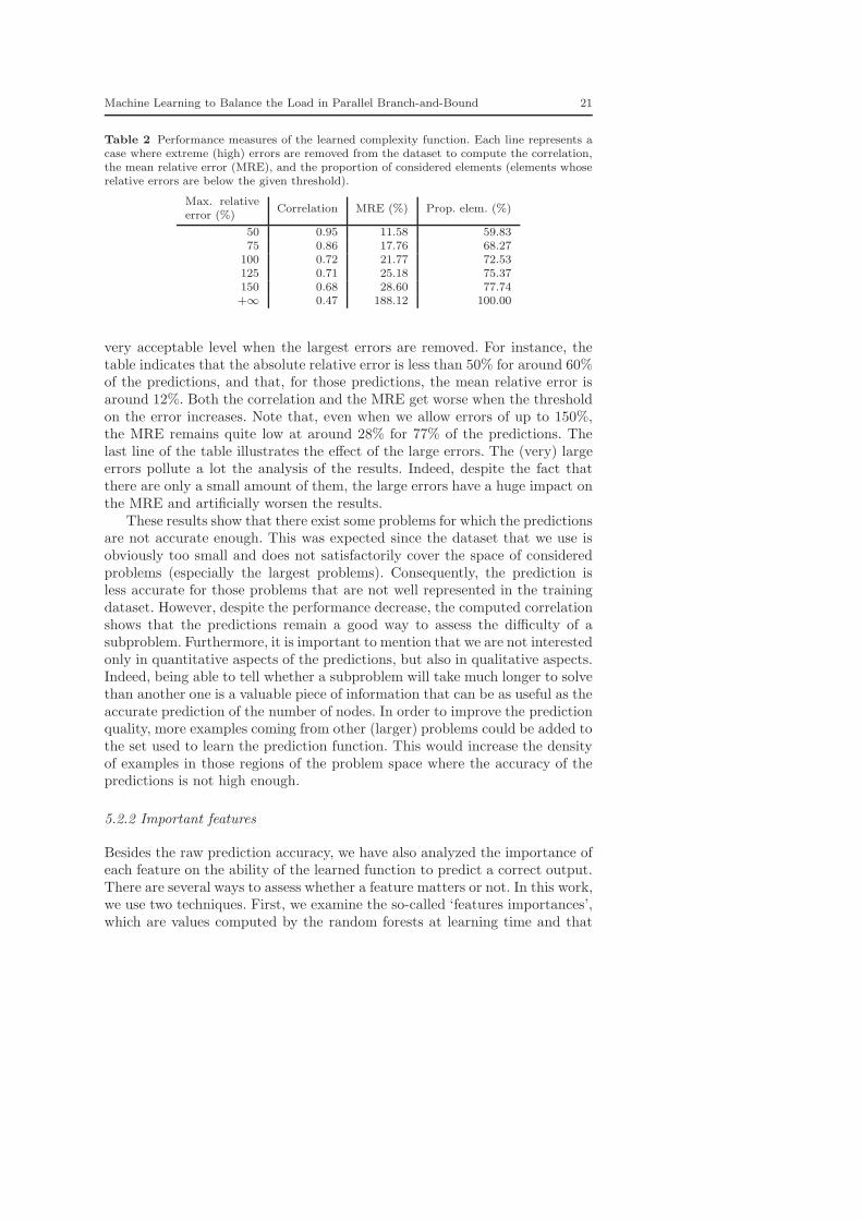
In Table 2, we assess the performances of our learned function by computingthe correlation and the mean relative error (MRE) between the predicted andreal values, where the MRE is computed as follows:
1
t
t∑
i=1
|ni − ni|max(1, ni)
.
In addition to computing the correlation and the MRE, we examine severalcases. Indeed, the distribution of the errors throughout the dataset is notuniform: the distribution is much denser for smaller errors. For that reason,we try to evaluate the learned function differently depending on the magnitudeof the errors. In order to do so, we successively consider a larger number ofpredictions. More specifically, we set a threshold on the relative error of eachpredicted value. Then, the extreme (highest) relative errors that are greaterthan the threshold are discarded from the set, and the performance measures(correlation and MRE) are computed from the remaining values. For instance,the first line of Table 2 represents the correlation and the MRE computed fromall predictions that differ by no more than 50% from the real value. The lastcolumn of the table indicates the proportion of values that are not discardedby the threshold, and, hence, the proportion of available values that are takeninto account for computing the performance measures.
The table shows that the learned function is able to catch the most im-portant dynamics of the subproblems. Indeed, the MRE is maintained at a
Machine Learning to Balance the Load in Parallel Branch-and-Bound 21
Table 2 Performance measures of the learned complexity function. Each line represents acase where extreme (high) errors are removed from the dataset to compute the correlation,the mean relative error (MRE), and the proportion of considered elements (elements whoserelative errors are below the given threshold).
Max. relativeerror (%)
Correlation MRE (%) Prop. elem. (%)
50 0.95 11.58 59.8375 0.86 17.76 68.27
100 0.72 21.77 72.53125 0.71 25.18 75.37150 0.68 28.60 77.74+∞ 0.47 188.12 100.00
very acceptable level when the largest errors are removed. For instance, thetable indicates that the absolute relative error is less than 50% for around 60%of the predictions, and that, for those predictions, the mean relative error isaround 12%. Both the correlation and the MRE get worse when the thresholdon the error increases. Note that, even when we allow errors of up to 150%,the MRE remains quite low at around 28% for 77% of the predictions. Thelast line of the table illustrates the effect of the large errors. The (very) largeerrors pollute a lot the analysis of the results. Indeed, despite the fact thatthere are only a small amount of them, the large errors have a huge impact onthe MRE and artificially worsen the results.
These results show that there exist some problems for which the predictionsare not accurate enough. This was expected since the dataset that we use isobviously too small and does not satisfactorily cover the space of consideredproblems (especially the largest problems). Consequently, the prediction isless accurate for those problems that are not well represented in the trainingdataset. However, despite the performance decrease, the computed correlationshows that the predictions remain a good way to assess the difficulty of asubproblem. Furthermore, it is important to mention that we are not interestedonly in quantitative aspects of the predictions, but also in qualitative aspects.Indeed, being able to tell whether a subproblem will take much longer to solvethan another one is a valuable piece of information that can be as useful as theaccurate prediction of the number of nodes. In order to improve the predictionquality, more examples coming from other (larger) problems could be added tothe set used to learn the prediction function. This would increase the densityof examples in those regions of the problem space where the accuracy of thepredictions is not high enough.
5.2.2 Important features
Besides the raw prediction accuracy, we have also analyzed the importance ofeach feature on the ability of the learned function to predict a correct output.There are several ways to assess whether a feature matters or not. In this work,we use two techniques. First, we examine the so-called ‘features importances’,which are values computed by the random forests at learning time and that

22 Marcos Alvarez, Wehenkel, Louveaux
sum to 1 over all features. The greater the feature importance, the more rele-vant the feature is. Similarly, we use the cost of omission (COO) (Otten andDechter 2012) to estimate the impact of a feature on the prediction ability.The cost of omission consists in omitting a given feature during the learningand the testing phases. We can then compute the estimated MRE obtainedwithout the chosen feature. The difference between the MRE obtained with-out the feature and the MRE obtained with all features is an image of howimportant the feature is. If the value of the COO is positive, this means thatthe feature is important for the prediction. On the other hand, when the COOis negative, it implies that the feature has a negative impact on the predictionaccuracy. Small values of the COO (either positive or negative) indicate thatthe feature is not very important and could just be a source of noise in theprediction. Note that we use in this work the normalized COO which consistsin attributing to the highest COO a value of 100, all other COOs being scaledaccordingly. Given that there exist some large errors than have a huge impacton the MRE, and, thus, on the COO, we compute the COOs for differentthresholds of the relative errors, just as in the previous section. The results ofthe features importances are summarized in Table 3 for the 10 most relevantfeatures.
The table indicates that feature #66, i.e., the gap decrease at the end ofthe probing phase, is very important. Also, and very interestingly, the impactof each feature seems to depend on the amplitude of the prediction errors.For instance, feature #18, i.e., the difference between the heuristic objectivevalue and the LP objective value at the root of the subproblem, seems im-portant for those values that are predicted quite accurately, but it becomesless relevant when larger errors are included in the computation of the COO.The same analysis can be carried out for all 10 features indicating that, al-though features #63, i.e., the maximum depth of the probing tree, and #66are clear winners when all predictions are considered, the other features areimportant too in different situations. However, it would be very interesting tofurther study the impact of some features, like features #14 (the minimum ofthe average objective increase for the unfixed variables), #18, and #62 (theratio between the number of unexplored and explored nodes after probing),on the performances of the parallel B&B, since it seems that removing themhas a positive impact on the prediction accuracy when the entire dataset isconsidered.
5.2.3 Parallel optimization
We now compare the approach that we propose to the trivial ones in a real par-allel optimization setting. We apply the three proposed partitioning schemes toour set of test problems and create increasingly larger partitions of their orig-inal optimization trees. Note that, in this case, the number of elements in thepartition is equal to the number of processors. We perform two types of exper-iments: with and without communications. In the case where communicationsare allowed, their sole purpose is to render the best primal bound available

Machine Learning to Balance the Load in Parallel Branch-and-Bound 23
Table 3 Features importances as computed by the random forests algorithm and normal-ized costs of omission for the 10 most important features.
Feat. #Feat.imp.
COO with threshold on max. allowed error (%)
50 75 100 125 150 +∞
63 0.6193 31.2 25.0 41.8 42.9 35.7 55.466 0.3529 -7.2 2.8 100.0 100.0 100.0 100.014 0.0052 9.7 -3.3 -2.3 -4.5 -10.9 -5.618 0.0043 100.0 100.0 -24.2 -30.1 -32.6 1.31 0.0041 4.6 -6.7 4.4 2.3 -0.7 -0.8
59 0.0031 3.5 -3.5 1.6 -2.6 -6.8 2.840 0.0017 4.8 -6.9 1.1 -0.9 -1.8 4.462 0.0014 20.1 8.1 12.5 9.2 5.8 -1.815 0.0011 5.1 -5.2 -0.7 -6.7 -6.5 1.161 0.0011 4.2 -8.9 5.5 9.0 10.9 1.6
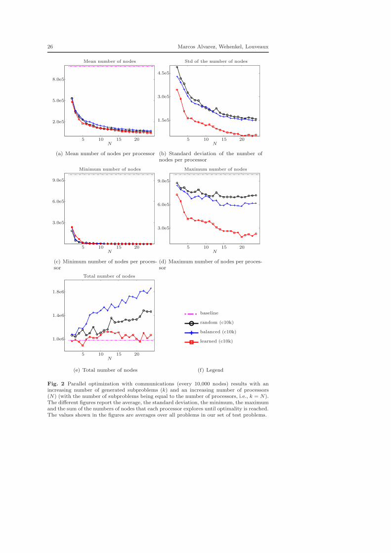
to all processes. The communication is thus maintained at its minimum butremains yet very useful to achieve good performances. The communicationworks as follows. There is, in shared memory, a single scalar that stores theobjective value of the best known integral solution. Every 10,000 nodes, eachprocessor reads the shared primal bound and updates its local primal boundaccordingly. This allows all processors to be aware of the best available so-lution in order to early prune unpromising branches of the tree. Moreover,each time a new integral solution is found, the processor responsible for thatdiscovery updates, if necessary, the shared primal bound. This mechanism isvery useful in reducing the total amount of work carried out by all processors,while being very light in terms of communications.
In our experiments, we generate a number of subproblems ranging from 2to 24, each subproblem being optimized by a single processor. At the end ofthe experiments, for each problem, the number of nodes explored by each pro-cessor is stored, and several measures (average, standard deviation, minimum,maximum, and sum) are computed from the stored values. These measures arefinally averaged over all problems in our test set and reported in Figures 1 and2 versus the number of generated subproblems. Figures 1 and 2 respectivelyreport the results without communications between the processors and withcommunications. We also report in the results a so-called ‘baseline’ which con-sists in the normal optimization of a problem, i.e., starting from the root, theproblem is solved to optimality by a single processor. Figures 1 and 2 are justmeant to show the trends of the performance measures. The detailed resultsare given in the form of tables in Appendix A.
A first observation that can be made from the reported results is that ourproposed approach, called ‘learned’, always beats the two trivial approachesin every aspect (considering the same communication setup). The results alsohighlight the importance of the communications to achieve good performancesin parallel B&B. Overall, the mean number of nodes per processor decreasesfor all partitioning schemes when the number of generated subproblems in-creases. The same observation can be made for the minimum of the number

24 Marcos Alvarez, Wehenkel, Louveaux
of nodes across all processors. The maximum of the number of nodes tendsto increase when the number of elements in the partition increases, but onlywhen communications are forbidden. This can be easily understood since thedeeper the subproblem is in the optimization tree, the less likely it is to con-tain a good feasible solution that can prune unpromising branches. Also notethat the maximum is the most interesting measure because it conditions thespeedup. Indeed, even if the total amount of work required to solve a prob-lem is not equal between the serial and the parallel case, the times neededto complete the optimization is conditioned by the processor that takes themost time. In order to analyze the potential speedups, the maximum numberof nodes must thus be compared with the number of nodes in the serial case,i.e., the baseline. The speedups obtained when communications are forbiddenare very modest. The situation is otherwise when we allow the processors tocommunicate. Indeed, in that case, our approach achieves a very interesting4.22 speedup in comparison with the serial case when the problem is paral-lelized on 24 cores. This has to be compared with the speedups of 1.36 and1.58 obtained with the random and balanced partitioning schemes. In otherwords, the approach that we propose indeed achieves speedups that can havean important impact in practice.
Moreover, it is important to emphasize that the computed speedups arelower bounds on the attainable speedups. Indeed, in this work, we do notperform dynamic load balancing since we only distribute the work to eachprocessor before the optimization starts. If a dynamic load balancing schemeis used to further improve the work equilibrium between the processors, it isconceivable that much higher speedups can be achieved. Indeed, in that case,other measures, such as the mean and the minimum numbers of nodes perprocessor, should be used to enrich our analysis. Given that the mean and theminimum workload per processor are both very low with our method, it isfair to expect greater gains in computation time if a dynamic load balancingscheme is used, together with our method, in order to redistribute the workfrom the busiest processor to idle ones.
Finally, the last set of experiments that we propose focuses on the paral-lel optimization of our set of test problems when the number k of generatedsubproblems is greater than the number N of processors. In order to do so,we generate a certain number k of subproblems with each considered parti-tioning scheme. Then, the subproblems are distributed across the N availableprocessors, either by randomly attributing k/N subproblems to each processor(for the random and balanced partitioning schemes), or by using Algorithm 2(for the learned partitioning scheme). Note that the number of subproblemsgenerated with the learned partitioning scheme is at most k, but may be lessgiven that Algorithm 1 provides another stopping criterion that can be usedto stop the generation of subproblems before the limit k is reached. Table 4 re-ports, in the case where the number of generated subproblems is greater thanthe number of processors, the same performance measures as those presentedin Figures 1 and 2. Note that, in this case, the performance measures (aver-age, standard deviation, etc.) are computed from the total number of nodes

Machine Learning to Balance the Load in Parallel Branch-and-Bound 25
5 10 15 20N
1.0e5
5.0e5
9.0e5
Mean number of nodes
(a) Mean number of nodes per processor
5 10 15 20N
0.5e6
1.0e6
1.5e6
Std of the number of nodes
(b) Standard deviation of the number ofnodes per processor
5 10 15 20N
2.5e5
5.0e5
7.5e5
Minimum number of nodes
(c) Minimum number of nodes per proces-sor
5 10 15 20N
1.0e6
3.0e6
5.0e6
Maximum number of nodes
(d) Maximum number of nodes per proces-sor
5 10 15 20N
0.2e7
1.0e7
1.8e7
Total number of nodes
(e) Total number of nodes
baseline
random
balanced
learned
(f) Legend
Fig. 1 Parallel optimization without communications results with an increasing number ofgenerated subproblems (k) and an increasing number of processors (N) (with the numberof subproblems being equal to the number of processors, i.e., k = N). The different figuresreport the average, the standard deviation, the minimum, the maximum and the sum of thenumbers of nodes that each processor explores until optimality is reached. The values shownin the figures are averages over all problems in our set of test problems.
26 Marcos Alvarez, Wehenkel, Louveaux
5 10 15 20N
2.0e5
5.0e5
8.0e5
Mean number of nodes
(a) Mean number of nodes per processor
5 10 15 20N
1.5e5
3.0e5
4.5e5
Std of the number of nodes
(b) Standard deviation of the number ofnodes per processor
5 10 15 20N
3.0e5
6.0e5
9.0e5
Minimum number of nodes
(c) Minimum number of nodes per proces-sor
5 10 15 20N
3.0e5
6.0e5
9.0e5
Maximum number of nodes
(d) Maximum number of nodes per proces-sor
5 10 15 20N
1.0e6
1.4e6
1.8e6
Total number of nodes
(e) Total number of nodes
baseline
random (c10k)
balanced (c10k)
learned (c10k)
(f) Legend
Fig. 2 Parallel optimization with communications (every 10,000 nodes) results with anincreasing number of generated subproblems (k) and an increasing number of processors(N) (with the number of subproblems being equal to the number of processors, i.e., k = N).The different figures report the average, the standard deviation, the minimum, the maximumand the sum of the numbers of nodes that each processor explores until optimality is reached.The values shown in the figures are averages over all problems in our set of test problems.

Machine Learning to Balance the Load in Parallel Branch-and-Bound 27
explored by each processor, which corresponds to the sum of the number ofnodes required by each subproblem attributed to the given worker. The totalnumber of nodes is thus an image of the total amount of work that a processorcarries out.
Table 4 indicates first that the parallel optimization without communica-tions does not compare very well with the single threaded case. Indeed, themaximum number of nodes that a processor performs is always greater thanin the single threaded case. This implies that the parallel optimization doesnot terminate before the single threaded B&B. However, the approach thatwe propose compares favorably with the trivial partitioning schemes. Indeed,with our method, the mean number of nodes that a processor explores de-creases, as well as the standard deviation. This implies that, on average, thenumber of nodes per processor is less than for a single threaded optimization.Things are different when communications are allowed between the proces-sors. Indeed, while the trivial partitioning schemes still perform very poorlycompared to the single threaded optimization, the proposed method, on theother hand, exhibits very interesting performances. Indeed, in that case, theobtained speedup between the single threaded baseline and the learned parti-tioning scheme is equal to 4.07 or 5.61, depending on the number of processors.Similarly to the case without communications, the mean number of nodes andthe standard deviation per processor are reduced compared to the trivial par-titioning schemes, which shows that the load is acceptably balanced betweenthe workers.
Finally, it is interesting to compare the situation where each processoris assigned only one subproblem, with the situation where each processor isresponsible for multiple subproblems. This analysis can be carried out by com-paring the results from Table 4 with those from Tables 5-9. Comparing bothsets of results for 12 and 24 processors yields the following observations. First,the mean and the total number of nodes are roughly equal between both se-tups. Additionally, we see that the standard deviation per processor decreaseswhen more subproblems are assigned to a single worker, which is a display ofbetter load balance. Lastly, we observe that the difference between the max-imum and the minimum number of nodes decreases when the processors areassigned more than one subproblem, which tends, again, to show that the workis better balanced in that case. Overall, the conclusion that can be drawn isthat allocating more than one subproblem to each processor does not increasethe total amount of work to be done, but sensibly reduces the unbalance be-tween the workers.
6 Conclusions and future work
In this paper, we proposed a new approach to split the optimization of a singleproblem into several parallel parts with the goal that the amount of work givento each processor is well balanced between the workers. The approach consistsin creating a complexity function, with the use of machine learning techniques,

28 Marcos Alvarez, Wehenkel, Louveaux
Table 4 Parallel optimization results when the number of generated subproblems (k) isgreater than the number of processors (N). The table reports the average, the standarddeviation, the minimum, the maximum and the sum (over all processors) of the numbersof nodes that each processor explores until optimality is reached. The values shown in thetables are averages over all problems in our set of test problems. Note that, for the learnedpartitioning scheme, the k indicates the maximum number of elements in the partition. Thereal number of generated subproblems is different for each problem and depends on thestopping criterion given in Algorithm 1.
N k Mean Std Min Max SumSingle 1 1 9.81e+05 - 9.81e+05 9.81e+05 9.81e+05
Without communicationrandom 12 240 7.94e+06 5.70e+06 1.73e+06 1.97e+07 9.53e+07random 24 480 6.29e+06 5.76e+06 1.00e+06 2.14e+07 1.51e+08
balanced 12 240 1.55e+07 8.81e+06 4.53e+06 3.33e+07 1.86e+08balanced 24 480 1.25e+07 8.15e+06 3.28e+06 3.79e+07 3.00e+08
learned 12 240 5.96e+05 2.38e+05 1.85e+05 9.89e+05 7.16e+06learned 24 480 5.54e+05 3.03e+05 1.22e+05 1.18e+06 1.33e+07
With communication (primal bound, every 10,000 nodes)random 12 240 1.67e+05 1.89e+05 4.22e+04 6.94e+05 2.00e+06random 24 480 7.98e+04 1.59e+05 1.03e+04 7.60e+05 1.91e+06
balanced 12 240 1.99e+05 1.50e+05 5.22e+04 5.47e+05 2.39e+06balanced 24 480 1.44e+05 1.27e+05 3.29e+04 5.73e+05 3.46e+06
learned 12 240 9.38e+04 6.14e+04 1.90e+04 2.41e+05 1.12e+06learned 24 480 4.58e+04 3.95e+04 6.80e+03 1.75e+05 1.10e+06
that is able to estimate the number of nodes, hence the amount of work, thata subproblem of the original problem requires in order to be fully optimized.To this end, we develop a set of features that are used to characterize a givensubproblem in the B&B tree, and use these features as input of the learnedcomplexity function in order to predict the expected number of nodes requiredto solve this subproblem to optimality. These estimates are then used to createa partition of the original optimization tree so that one or several elements ofthe partition can be given to each processor. The experiments show that ourapproach succeeds in balancing the amount of work between the processorsand that interesting speedups can be achieved with little effort.
Further research orientations include the development of more relevant fea-tures that would better grasp the dynamics of the considered problems in orderto better predict the subproblem size. Another research direction is to imple-ment the proposed framework on massively parallel computers to understandhow the speedups and processor utilizations change when the original work issplit into a very large number of independent parts.
Finally, let us emphasize the fact that, although, in this paper, we totallyfocus on a single class of MIP problems, the same framework can be transposedto any class of problems with minor adaptations of the proposed features.
Acknowledgements This work was funded by the Dysco Interuniversity Attraction Pole(IAP) of the Belgian Science Policy Office and the Pascal2 Network of Excellence of theEuropean Union. AMA’s thesis is funded by a FRIA scholarship from the Fonds de la

Machine Learning to Balance the Load in Parallel Branch-and-Bound 29
Recherche Scientifique-FNRS (F.R.S.-FNRS). The scientific responsibility rests with theauthors.
References
Breiman L (2001) Random forests. Machine learning 45(1):5–32Dorta I, Leon C, Rodriguez C (2004) Parallel branch-and-bound skeletons: Message passing
and shared memory implementations. In: Parallel Processing and Applied Mathematics,Springer, pp 286–291
Eckstein J, Phillips CA, Hart WE (2001) Pico: An object-oriented framework for parallelbranch and bound. Studies in Computational Mathematics 8:219–265
El-Dessouki OI, Huen WH (1980) Distributed enumeration on between computers. IEEETransactions on Computers 29(9):818–825
Gendron B, Crainic TG (1994) Parallel branch-and-branch algorithms: Survey and synthesis.Operations Research 42(6):1042–1066
Karp R, Zhang Y (1988) A randomized parallel branch-and-bound procedure. In: Proceed-ings of the twentieth annual ACM symposium on Theory of computing, ACM, pp 290–300
Kumar V, Rao VN (1987) Parallel depth first search. part ii. analysis. International Journalof Parallel Programming 16(6):501–519
Lai TH, Sahni S (1984) Anomalies in parallel branch-and-bound algorithms. Communica-tions of the ACM 27(6):594–602
Laursen PS (1994) Can parallel branch and bound without communication be effective?SIAM Journal on Optimization 4(2):288–296
Linderoth JT (1998) Topics in parallel integer optimization. PhD thesis, Georgia Instituteof Technology
Otten L, Dechter R (2012) A case study in complexity estimation: Towards parallel branch-and-bound over graphical models. In: Proceedings of the Twenty-Eighth Conference onUncertainty in Artificial Intelligence, pp 665–674
Pruul E, Nemhauser G, Rushmeier R (1988) Branch-and-bound and parallel computation:A historical note. Operations Research Letters 7(2):65–69
Rao VN, Kumar V (1987) Parallel depth first search. part i. implementation. InternationalJournal of Parallel Programming 16(6):479–499
Wah B, Yu CF (1985) Stochastic modeling of branch-and-bound algorithms with best-firstsearch. Software Engineering, IEEE Transactions on SE-11(9):922–934
Yang MK, Das CR (1994) Evaluation of a parallel branch-and-bound algorithm on a classof multiprocessors. Parallel and Distributed Systems, IEEE Transactions on 5(1):74–86

30 Marcos Alvarez, Wehenkel, Louveaux
A Complete experimental results
This appendix contains the detailed experimental results obtained when our test problemsare optimized by a parallel B&B. We report the mean, standard deviation, minimum, andmaximum numbers of nodes observed on each processor, together with the sum of the numberof nodes of each processor. The results are then averaged for all problems and reported inthe following tables. Note that, in this case, the number k of generated subproblems is equalto the number N of processors.
Table 5 Mean number of nodes
Without comm. With comm. (every 10k nodes)N baseline random balanced learned random balanced learned2 9.81e+05 7.27e+05 1.01e+06 5.62e+05 5.31e+05 5.42e+05 4.82e+053 9.81e+05 5.58e+05 8.11e+05 4.03e+05 3.48e+05 3.59e+05 3.30e+054 9.81e+05 5.29e+05 8.91e+05 3.27e+05 2.75e+05 2.97e+05 2.39e+055 9.81e+05 5.22e+05 8.07e+05 2.86e+05 2.32e+05 2.36e+05 1.78e+056 9.81e+05 4.75e+05 7.98e+05 2.56e+05 1.78e+05 2.09e+05 1.66e+057 9.81e+05 4.91e+05 9.59e+05 2.28e+05 1.57e+05 2.01e+05 1.48e+058 9.81e+05 4.64e+05 1.18e+06 1.96e+05 1.51e+05 1.81e+05 1.32e+059 9.81e+05 4.74e+05 1.08e+06 1.93e+05 1.20e+05 1.60e+05 1.16e+05
10 9.81e+05 4.68e+05 1.06e+06 2.14e+05 1.11e+05 1.49e+05 1.09e+0511 9.81e+05 4.84e+05 1.02e+06 2.02e+05 1.04e+05 1.40e+05 1.04e+0512 9.81e+05 4.94e+05 1.04e+06 2.22e+05 9.69e+04 1.24e+05 9.57e+0413 9.81e+05 6.74e+05 1.05e+06 1.53e+05 1.04e+05 1.23e+05 8.86e+0414 9.81e+05 6.60e+05 1.05e+06 1.45e+05 9.17e+04 1.09e+05 7.99e+0415 9.81e+05 6.51e+05 1.10e+06 1.36e+05 8.62e+04 1.03e+05 7.60e+0416 9.81e+05 6.29e+05 1.10e+06 1.28e+05 8.11e+04 1.04e+05 6.46e+0417 9.81e+05 6.14e+05 1.06e+06 1.24e+05 7.82e+04 9.48e+04 6.40e+0418 9.81e+05 5.93e+05 1.02e+06 1.96e+05 7.32e+04 9.61e+04 5.82e+0419 9.81e+05 5.71e+05 1.00e+06 1.92e+05 7.02e+04 9.05e+04 5.70e+0420 9.81e+05 5.72e+05 9.74e+05 1.87e+05 6.66e+04 8.45e+04 5.12e+0421 9.81e+05 5.60e+05 7.96e+05 2.06e+05 6.58e+04 8.59e+04 4.67e+0422 9.81e+05 5.56e+05 7.77e+05 2.06e+05 6.75e+04 8.27e+04 5.14e+0423 9.81e+05 6.10e+05 5.21e+05 2.06e+05 6.38e+04 7.74e+04 4.54e+0424 9.81e+05 6.08e+05 3.37e+05 2.06e+05 6.11e+04 7.77e+04 4.61e+04
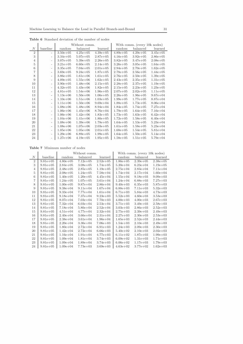
Machine Learning to Balance the Load in Parallel Branch-and-Bound 31
Table 6 Standard deviation of the number of nodes
Without comm. With comm. (every 10k nodes)N baseline random balanced learned random balanced learned2 - 3.50e+05 4.25e+05 4.39e+05 4.89e+05 4.29e+05 3.45e+053 - 3.34e+05 5.07e+05 2.87e+05 4.16e+05 3.92e+05 2.86e+054 - 3.07e+05 5.39e+05 2.26e+05 3.82e+05 3.47e+05 2.08e+055 - 3.21e+05 6.60e+05 2.14e+05 3.26e+05 3.05e+05 1.64e+056 - 3.35e+05 7.04e+05 2.01e+05 2.94e+05 2.70e+05 1.62e+057 - 3.69e+05 9.24e+05 1.87e+05 2.78e+05 2.56e+05 1.44e+058 - 3.86e+05 1.61e+06 1.61e+05 2.76e+05 2.50e+05 1.39e+059 - 4.09e+05 1.55e+06 1.62e+05 2.43e+05 2.35e+05 1.31e+05
10 - 3.90e+05 1.48e+06 2.15e+05 2.28e+05 2.37e+05 1.19e+0511 - 4.32e+05 1.43e+06 1.82e+05 2.15e+05 2.23e+05 1.23e+0512 - 4.81e+05 1.54e+06 1.96e+05 2.07e+05 2.02e+05 1.11e+0513 - 1.13e+06 1.50e+06 1.06e+05 2.26e+05 1.96e+05 9.67e+0414 - 1.10e+06 1.51e+06 1.03e+05 1.99e+05 1.77e+05 8.87e+0415 - 1.11e+06 1.50e+06 9.69e+04 1.88e+05 1.73e+05 8.06e+0416 - 1.08e+06 1.48e+06 8.94e+04 1.84e+05 1.74e+05 7.27e+0417 - 1.06e+06 1.45e+06 8.76e+04 1.79e+05 1.64e+05 7.16e+0418 - 1.06e+06 1.42e+06 1.83e+05 1.73e+05 1.63e+05 6.42e+0419 - 1.04e+06 1.41e+06 1.80e+05 1.72e+05 1.58e+05 6.40e+0420 - 1.08e+06 1.39e+06 1.78e+05 1.64e+05 1.53e+05 5.23e+0421 - 1.08e+06 1.07e+06 2.03e+05 1.61e+05 1.58e+05 5.23e+0422 - 1.05e+06 1.05e+06 2.01e+05 1.68e+05 1.54e+05 5.81e+0423 - 1.29e+06 6.89e+05 1.99e+05 1.64e+05 1.50e+05 5.14e+0424 - 1.27e+06 4.19e+05 1.95e+05 1.58e+05 1.51e+05 5.79e+04
Table 7 Minimum number of nodes
Without comm. With comm. (every 10k nodes)N baseline random balanced learned random balanced learned2 9.81e+05 4.80e+05 7.12e+05 2.52e+05 1.86e+05 2.39e+05 2.38e+053 9.81e+05 2.84e+05 3.08e+05 1.74e+05 5.20e+04 6.23e+04 1.19e+054 9.81e+05 2.48e+05 2.85e+05 1.19e+05 2.75e+04 2.83e+04 7.11e+045 9.81e+05 2.08e+05 1.24e+05 7.58e+04 1.74e+04 2.17e+04 1.60e+046 9.81e+05 1.40e+05 1.20e+05 4.45e+04 1.55e+04 9.18e+03 9.09e+037 9.81e+05 1.24e+05 1.07e+05 3.61e+04 1.24e+04 6.88e+03 7.27e+038 9.81e+05 1.00e+05 9.87e+04 2.86e+04 9.40e+03 6.35e+03 5.87e+039 9.81e+05 9.38e+04 9.11e+04 1.67e+04 6.88e+03 7.11e+03 5.32e+03
10 9.81e+05 9.33e+04 7.77e+04 1.61e+04 6.71e+03 5.84e+03 4.73e+0311 9.81e+05 9.18e+04 7.37e+04 9.23e+03 5.52e+03 4.60e+03 3.53e+0312 9.81e+05 8.07e+04 7.03e+04 7.70e+03 4.00e+03 4.00e+03 2.67e+0313 9.81e+05 7.32e+04 6.03e+04 2.53e+04 3.71e+03 3.49e+03 2.58e+0314 9.81e+05 7.18e+04 5.80e+04 2.52e+04 3.03e+03 2.86e+03 2.52e+0315 9.81e+05 4.51e+04 4.77e+04 2.32e+04 2.75e+03 2.39e+03 2.49e+0316 9.81e+05 2.40e+04 3.66e+04 2.31e+04 2.27e+03 2.30e+03 2.53e+0317 9.81e+05 2.38e+04 3.61e+04 1.96e+04 1.65e+03 2.52e+03 2.44e+0318 9.81e+05 2.20e+04 3.36e+04 7.06e+03 1.54e+03 2.10e+03 2.49e+0319 9.81e+05 1.80e+04 2.72e+04 6.91e+03 1.24e+03 2.09e+03 2.30e+0320 9.81e+05 1.42e+04 2.72e+04 6.66e+03 5.40e+02 2.10e+03 2.02e+0321 9.81e+05 1.16e+04 1.91e+04 4.77e+03 6.11e+02 1.87e+03 1.99e+0322 9.81e+05 1.09e+04 1.81e+04 3.74e+03 6.09e+02 1.31e+03 1.71e+0323 9.81e+05 1.09e+04 1.89e+04 3.74e+03 6.06e+02 1.17e+03 1.79e+0324 9.81e+05 1.09e+04 7.73e+03 3.69e+03 4.63e+02 3.77e+02 1.62e+03
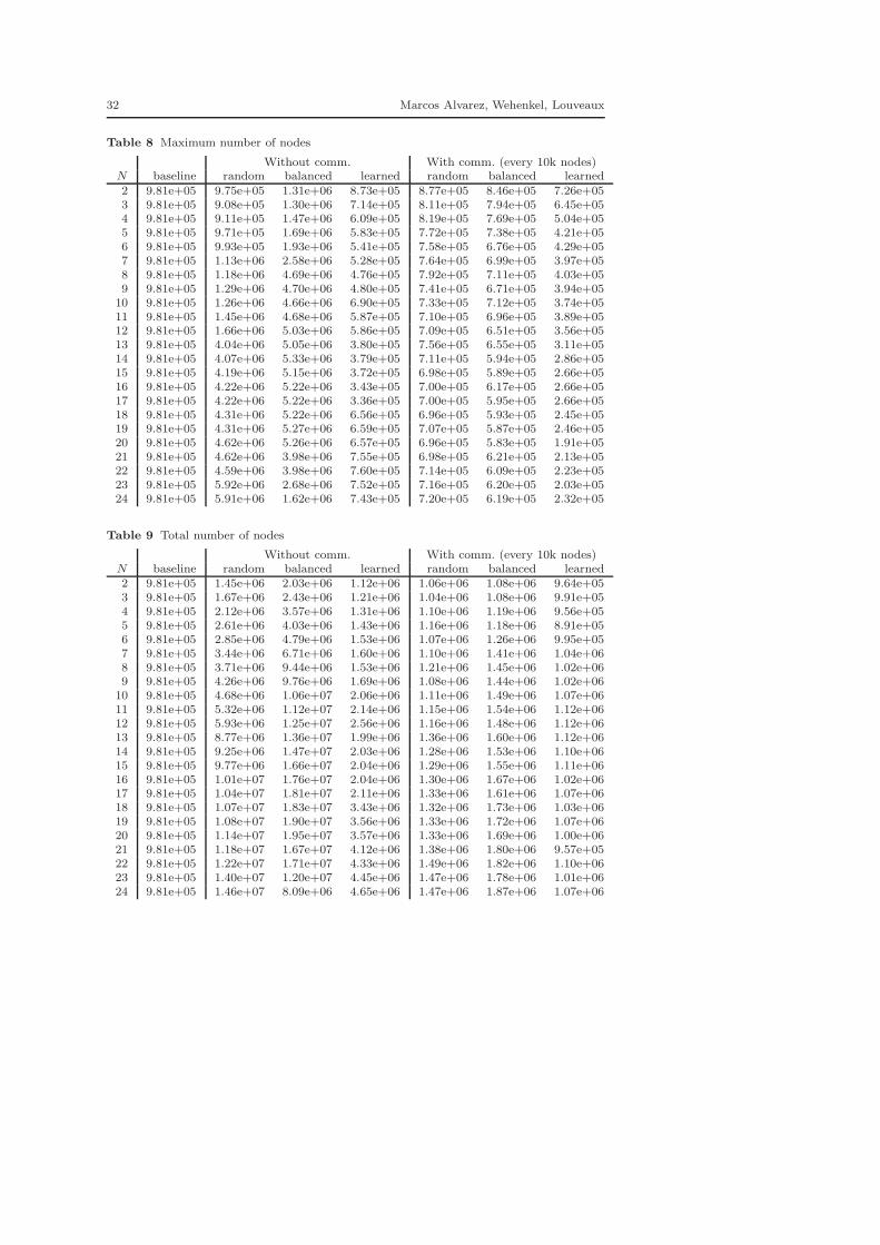
32 Marcos Alvarez, Wehenkel, Louveaux
Table 8 Maximum number of nodes
Without comm. With comm. (every 10k nodes)N baseline random balanced learned random balanced learned2 9.81e+05 9.75e+05 1.31e+06 8.73e+05 8.77e+05 8.46e+05 7.26e+053 9.81e+05 9.08e+05 1.30e+06 7.14e+05 8.11e+05 7.94e+05 6.45e+054 9.81e+05 9.11e+05 1.47e+06 6.09e+05 8.19e+05 7.69e+05 5.04e+055 9.81e+05 9.71e+05 1.69e+06 5.83e+05 7.72e+05 7.38e+05 4.21e+056 9.81e+05 9.93e+05 1.93e+06 5.41e+05 7.58e+05 6.76e+05 4.29e+057 9.81e+05 1.13e+06 2.58e+06 5.28e+05 7.64e+05 6.99e+05 3.97e+058 9.81e+05 1.18e+06 4.69e+06 4.76e+05 7.92e+05 7.11e+05 4.03e+059 9.81e+05 1.29e+06 4.70e+06 4.80e+05 7.41e+05 6.71e+05 3.94e+05
10 9.81e+05 1.26e+06 4.66e+06 6.90e+05 7.33e+05 7.12e+05 3.74e+0511 9.81e+05 1.45e+06 4.68e+06 5.87e+05 7.10e+05 6.96e+05 3.89e+0512 9.81e+05 1.66e+06 5.03e+06 5.86e+05 7.09e+05 6.51e+05 3.56e+0513 9.81e+05 4.04e+06 5.05e+06 3.80e+05 7.56e+05 6.55e+05 3.11e+0514 9.81e+05 4.07e+06 5.33e+06 3.79e+05 7.11e+05 5.94e+05 2.86e+0515 9.81e+05 4.19e+06 5.15e+06 3.72e+05 6.98e+05 5.89e+05 2.66e+0516 9.81e+05 4.22e+06 5.22e+06 3.43e+05 7.00e+05 6.17e+05 2.66e+0517 9.81e+05 4.22e+06 5.22e+06 3.36e+05 7.00e+05 5.95e+05 2.66e+0518 9.81e+05 4.31e+06 5.22e+06 6.56e+05 6.96e+05 5.93e+05 2.45e+0519 9.81e+05 4.31e+06 5.27e+06 6.59e+05 7.07e+05 5.87e+05 2.46e+0520 9.81e+05 4.62e+06 5.26e+06 6.57e+05 6.96e+05 5.83e+05 1.91e+0521 9.81e+05 4.62e+06 3.98e+06 7.55e+05 6.98e+05 6.21e+05 2.13e+0522 9.81e+05 4.59e+06 3.98e+06 7.60e+05 7.14e+05 6.09e+05 2.23e+0523 9.81e+05 5.92e+06 2.68e+06 7.52e+05 7.16e+05 6.20e+05 2.03e+0524 9.81e+05 5.91e+06 1.62e+06 7.43e+05 7.20e+05 6.19e+05 2.32e+05
Table 9 Total number of nodes
Without comm. With comm. (every 10k nodes)N baseline random balanced learned random balanced learned2 9.81e+05 1.45e+06 2.03e+06 1.12e+06 1.06e+06 1.08e+06 9.64e+053 9.81e+05 1.67e+06 2.43e+06 1.21e+06 1.04e+06 1.08e+06 9.91e+054 9.81e+05 2.12e+06 3.57e+06 1.31e+06 1.10e+06 1.19e+06 9.56e+055 9.81e+05 2.61e+06 4.03e+06 1.43e+06 1.16e+06 1.18e+06 8.91e+056 9.81e+05 2.85e+06 4.79e+06 1.53e+06 1.07e+06 1.26e+06 9.95e+057 9.81e+05 3.44e+06 6.71e+06 1.60e+06 1.10e+06 1.41e+06 1.04e+068 9.81e+05 3.71e+06 9.44e+06 1.53e+06 1.21e+06 1.45e+06 1.02e+069 9.81e+05 4.26e+06 9.76e+06 1.69e+06 1.08e+06 1.44e+06 1.02e+06
10 9.81e+05 4.68e+06 1.06e+07 2.06e+06 1.11e+06 1.49e+06 1.07e+0611 9.81e+05 5.32e+06 1.12e+07 2.14e+06 1.15e+06 1.54e+06 1.12e+0612 9.81e+05 5.93e+06 1.25e+07 2.56e+06 1.16e+06 1.48e+06 1.12e+0613 9.81e+05 8.77e+06 1.36e+07 1.99e+06 1.36e+06 1.60e+06 1.12e+0614 9.81e+05 9.25e+06 1.47e+07 2.03e+06 1.28e+06 1.53e+06 1.10e+0615 9.81e+05 9.77e+06 1.66e+07 2.04e+06 1.29e+06 1.55e+06 1.11e+0616 9.81e+05 1.01e+07 1.76e+07 2.04e+06 1.30e+06 1.67e+06 1.02e+0617 9.81e+05 1.04e+07 1.81e+07 2.11e+06 1.33e+06 1.61e+06 1.07e+0618 9.81e+05 1.07e+07 1.83e+07 3.43e+06 1.32e+06 1.73e+06 1.03e+0619 9.81e+05 1.08e+07 1.90e+07 3.56e+06 1.33e+06 1.72e+06 1.07e+0620 9.81e+05 1.14e+07 1.95e+07 3.57e+06 1.33e+06 1.69e+06 1.00e+0621 9.81e+05 1.18e+07 1.67e+07 4.12e+06 1.38e+06 1.80e+06 9.57e+0522 9.81e+05 1.22e+07 1.71e+07 4.33e+06 1.49e+06 1.82e+06 1.10e+0623 9.81e+05 1.40e+07 1.20e+07 4.45e+06 1.47e+06 1.78e+06 1.01e+0624 9.81e+05 1.46e+07 8.09e+06 4.65e+06 1.47e+06 1.87e+06 1.07e+06