machine learning - python course · python tutorial: a tutorial http ... the algorithm for the...

Machine Learning

Bernd Klein

February, 2018

Python Tutorial: A Tutorial http://localhost/projects/python-course.eu/total_l...

1 of 113 2/21/18, 12:51 PM

T U T O R I A L A N D O N L I N E C O U R S E


2 of 113 2/21/18, 12:51 PM

M A C H I N E L E A R N I N G

This is a completely new and incomplete chapter of our tutorial! Westarted work in January 2017!

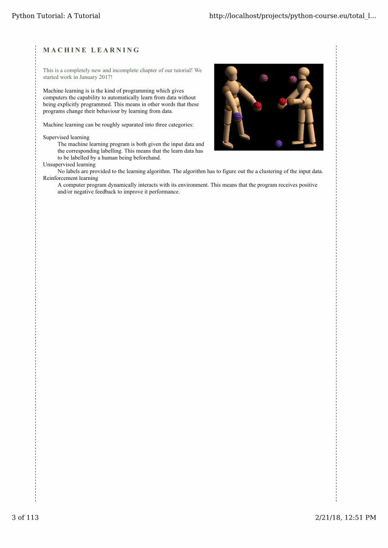
Machine learning is is the kind of programming which givescomputers the capability to automatically learn from data withoutbeing explicitly programmed. This means in other words that theseprograms change their behaviour by learning from data.

Machine learning can be roughly separated into three categories:

Supervised learningThe machine learning program is both given the input data andthe corresponding labelling. This means that the learn data hasto be labelled by a human being beforehand.

Unsupervised learningNo labels are provided to the learning algorithm. The algorithm has to figure out the a clustering of the input data.

Reinforcement learningA computer program dynamically interacts with its environment. This means that the program receives positiveand/or negative feedback to improve it performance.


3 of 113 2/21/18, 12:51 PM

M A C H I N E L E A R N I N G T E R M I N O L O G Y

CLASSIFIER

A program or a function which maps fromunlabeled instances to classes is called aclassifier.

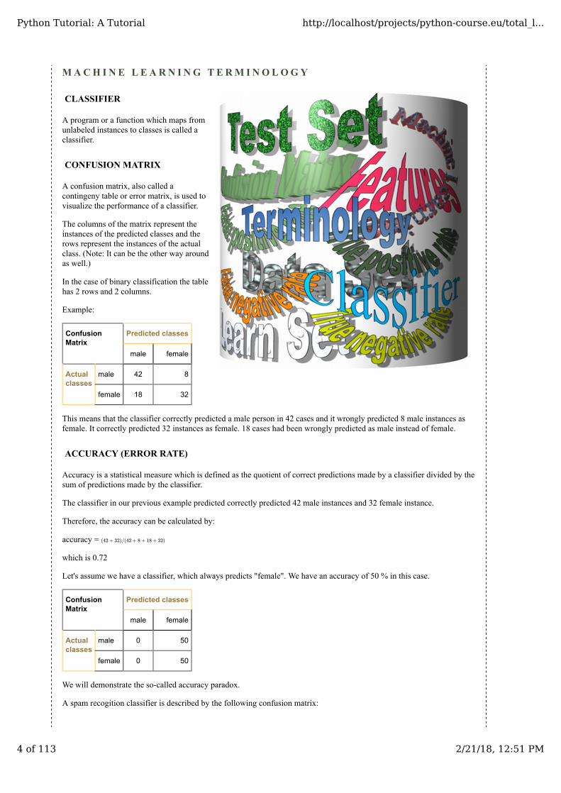
CONFUSION MATRIX

A confusion matrix, also called acontingeny table or error matrix, is used tovisualize the performance of a classifier.

The columns of the matrix represent theinstances of the predicted classes and therows represent the instances of the actualclass. (Note: It can be the other way aroundas well.)

In the case of binary classification the tablehas 2 rows and 2 columns.

Example:

ConfusionMatrix

Predicted classes

male female

Actualclasses

male 42 8

female 18 32

This means that the classifier correctly predicted a male person in 42 cases and it wrongly predicted 8 male instances asfemale. It correctly predicted 32 instances as female. 18 cases had been wrongly predicted as male instead of female.

ACCURACY (ERROR RATE)

Accuracy is a statistical measure which is defined as the quotient of correct predictions made by a classifier divided by thesum of predictions made by the classifier.

The classifier in our previous example predicted correctly predicted 42 male instances and 32 female instance.

Therefore, the accuracy can be calculated by:

accuracy =

which is 0.72

Let's assume we have a classifier, which always predicts "female". We have an accuracy of 50 % in this case.

ConfusionMatrix

Predicted classes

male female

Actualclasses

male 0 50

female 0 50

We will demonstrate the so-called accuracy paradox.

A spam recogition classifier is described by the following confusion matrix:

(42 + 32)/(42 + 8 + 18 + 32)


4 of 113 2/21/18, 12:51 PM

ConfusionMatrix

Predicted classes

spam ham

Actualclasses

spam 4 1

ham 4 91

The accuracy of this classifier is (4 + 91) / 100, i.e. 95 %.

The following classifier predicts solely "ham" and has the same accuracy.

ConfusionMatrix

Predicted classes

spam ham

Actualclasses

spam 0 5

ham 0 95

The accuracy of this classifier is 95%, even though it is not capable of recognizing any spam at all.

PRECISION AND RECALL

ConfusionMatrix

Predicted classes

negative positive

Actualclasses

negative TN FP

positive FN TP

Accuracy:

Precision:

Recall:

SUPERVISED LEARNING

The machine learning program is both given the input data and the corresponding labelling. This means that the learn datahas to be labelled by a human being beforehand.

UNSUPERVISED LEARNING

No labels are provided to the learning algorithm. The algorithm has to figure out the a clustering of the input data.

REINFORCEMENT LEARNING

A computer program dynamically interacts with its environment. This means that the program receives positive and/ornegative feedback to improve it performance.

(TN + TP)/(TN + TP + FN + FP)

TP/(TP + FP)

TP/(TP + FN)


5 of 113 2/21/18, 12:51 PM

K - N E A R E S T- N E I G H B O R C L A S S I F I E R

"Show me who your friends are and I’ll tellyou who you are?"

The concept of the k-nearest neighborclassifier can hardly be simpler described.This is an old saying, which can be foundin many languages and many cultures. It'salso metnioned in other words in the Bible:"He who walks with wise men will bewise, but the companion of fools willsuffer harm" (Proverbs 13:20 )

This means that the concept of thek-nearest neighbor classifier is part of oureveryday life and judging: Imagine youmeet a group of people, they are all veryyoung, stylish and sportive. They talkabout there friend Ben, who isn't withthem. So, what is your imagination of Ben?Right, you imagine him as being yong,stylish and sportive as well.

If you learn that Ben lives in aneighborhood where people vote conservative and that the average income is above 200000 dollars a year? Both hisneighbors make even more than 300,000 dollars per year? What do you think of Ben? Most probably, you do not considerhim to be an underdog and you may suspect him to be a conservative as well?

Now let's get a little bit more mathematically:

The k-Nearest-Neighbor Classifier (k-NN) works directly on the learned samples, instead of creating rules compared toother classification methods.

Nearest Neighbor Algorithm:

Given a set of categories , also called classes, e.g. {"male", "female"}. There is also a learnset consisting oflabelled instances.

The task of classification consists in assigning a category or class to an arbitrary instance. If the instance is an element of, the label of the instance will be used.

Now, we will look at the case where is not in :

is compared with all instances of . A distance metric is used for comparison. We determine the closest neighbors of ,i.e. the items with the smallest distances. is a user defined constant and a positive integer, which is usually small.

The most common class of will be assigned to the instance . If k = 1, then the object is simply assigned to the class ofthat single nearest neighbor.

The algorithm for the k-nearest neighbor classifier is among the simplest of all machine learning algorithms. k-NN is atype of instance-based learning, or lazy learning, where the function is only approximated locally and all the computationsare performed, when we do the actual classification.

K-NEAREST-NEIGHBOR FROM SCRATCH

PREPARING THE DATASET

{ , , . . . }c1 c2 cn LS

o

LS

o LS

o LS k o

k

LS o


6 of 113 2/21/18, 12:51 PM

Before we actually start with writing a nearest neighbor classifier, we need to think about the data, i.e. the learnset. Wewill use the "iris" dataset provided by the datasets of the sklearn module.

The data set consists of 50 samples from each of three species of Iris

Iris setosa,Iris virginica andIris versicolor.

Four features were measured from each sample: the length and the width of the sepals and petals, in centimetres.

import numpy as npfrom sklearn import datasetsiris = datasets.load_iris()iris_data = iris.datairis_labels = iris.targetprint(iris_data[0], iris_data[79], iris_data[100])print(iris_labels[0], iris_labels[79], iris_labels[100])

The previous Python code returned the following result:

[ 5.1 3.5 1.4 0.2] [ 5.7 2.6 3.5 1. ] [ 6.3 3.3 6. 2.5]0 1 2

We create a learnset from the sets above. We use permutation from np.random to split the data randomly.

np.random.seed(42)indices = np.random.permutation(len(iris_data))n_training_samples = 12learnset_data = iris_data[indices[:-n_training_samples]]learnset_labels = iris_labels[indices[:-n_training_samples]]testset_data = iris_data[indices[-n_training_samples:]]testset_labels = iris_labels[indices[-n_training_samples:]]print(learnset_data[:4], learnset_labels[:4])print(testset_data[:4], testset_labels[:4])

The previous Python code returned the following:

[[ 6.1 2.8 4.7 1.2] [ 5.7 3.8 1.7 0.3] [ 7.7 2.6 6.9 2.3] [ 6. 2.9 4.5 1.5]] [1 0 2 1][[ 5.7 2.8 4.1 1.3] [ 6.5 3. 5.5 1.8] [ 6.3 2.3 4.4 1.3] [ 6.4 2.9 4.3 1.3]] [1 2 1 1]

The following code is only necessary to visualize the data of our learnset. Our data consists of for values per iris item, so


7 of 113 2/21/18, 12:51 PM

we will reduce the data to three values by summing up the third and fourth value. This way, we are capable of depictingthe data in 3-dimensional space:

# following line is only necessary, if you use ipython notebook!!!%matplotlib inlineimport matplotlib.pyplot as pltfrom mpl_toolkits.mplot3d import Axes3Dcolours = ("r", "b")X = []for iclass in range(3):

X.append([[], [], []])for i in range(len(learnset_data)):

if learnset_labels[i] == iclass:X[iclass][0].append(learnset_data[i][0])X[iclass][1].append(learnset_data[i][1])X[iclass][2].append(sum(learnset_data[i][2:]))

colours = ("r", "g", "y")fig = plt.figure()ax = fig.add_subplot(111, projection='3d')for iclass in range(3):

ax.scatter(X[iclass][0], X[iclass][1], X[iclass][2], c=colours[iclass])plt.show()

DETERMINING THE NEIGHBORS

To determine the similarity between two instances, we need a distance function. In our example, the Euclidean distance isideal:

def distance(instance1, instance2):# just in case, if the instances are lists or tuples:instance1 = np.array(instance1)instance2 = np.array(instance2)

return np.linalg.norm(instance1 - instance2)

print(distance([3, 5], [1, 1]))print(distance(learnset_data[3], learnset_data[44]))

This gets us the following result:

4.4721359553.41906419946

The function 'get_neighbors returns a list with 'k' neighbors, which are closest to the instance 'test_instance':

def get_neighbors(training_set,labels,test_instance,k,distance=distance):

""" get_neighors calculates a list of the k nearest neighbors of an instance 'test_instance'.


8 of 113 2/21/18, 12:51 PM

The list neighbors contains 3-tuples with (index, dist, label) where index is the index from the training_set, dist is the distance between the test_instance and the instance training_set[index] distance is a reference to a function used to calculate the distances """

distances = []for index in range(len(training_set)):

dist = distance(test_instance, training_set[index])distances.append((training_set[index], dist, labels[index]))

distances.sort(key=lambda x: x[1])neighbors = distances[:k]return neighbors

We will test the function with our iris samples:

for i in range(5):neighbors = get_neighbors(learnset_data,

learnset_labels,testset_data[i],3,distance=distance)

print(i,testset_data[i],testset_labels[i],neighbors)

The previous Python code returned the following output:

0 [ 5.7 2.8 4.1 1.3] 1 [(array([ 5.7, 2.9, 4.2, 1.3]), 0.14142135623730995, 1), (array([ 5.6, 2.7, 4.2, 1.3]), 0.17320508075688815, 1), (array([ 5.6, 3. , 4.1, 1.3]), 0.22360679774997935, 1)]1 [ 6.5 3. 5.5 1.8] 2 [(array([ 6.4, 3.1, 5.5, 1.8]), 0.14142135623730931, 2), (array([ 6.3, 2.9, 5.6, 1.8]), 0.24494897427831783, 2), (array([ 6.5, 3. , 5.2, 2. ]), 0.36055512754639879, 2)]2 [ 6.3 2.3 4.4 1.3] 1 [(array([ 6.2, 2.2, 4.5, 1.5]), 0.26457513110645864, 1), (array([ 6.3, 2.5, 4.9, 1.5]), 0.57445626465380295, 1), (array([ 6. , 2.2, 4. , 1. ]), 0.5916079783099617, 1)]3 [ 6.4 2.9 4.3 1.3] 1 [(array([ 6.2, 2.9, 4.3, 1.3]), 0.20000000000000018, 1), (array([ 6.6, 3. , 4.4, 1.4]), 0.26457513110645869, 1), (array([ 6.6, 2.9, 4.6, 1.3]), 0.3605551275463984, 1)]4 [ 5.6 2.8 4.9 2. ] 2 [(array([ 5.8, 2.7, 5.1, 1.9]), 0.31622776601683755, 2), (array([ 5.8, 2.7, 5.1, 1.9]), 0.31622776601683755, 2), (array([ 5.7, 2.5, 5. , 2. ]), 0.33166247903553986, 2)]

VOTING TO GET A SINGLE RESULT

We will write a vote function now. This functions uses the class 'Counter' from collections to count the quantity of theclasses inside of an instance list. This instance list will be the neighbors of course. The function 'vote' returns the mostcommon class:

from collections import Counterdef vote(neighbors):

class_counter = Counter()for neighbor in neighbors:

class_counter[neighbor[2]] += 1


9 of 113 2/21/18, 12:51 PM

return class_counter.most_common(1)[0][0]

We will test 'vote' on our training samples:

for i in range(n_training_samples):neighbors = get_neighbors(learnset_data,


print("index: ", i,", result of vote: ", vote(neighbors),", label: ", testset_labels[i],", data: ", testset_data[i])


index: 0 , result of vote: 1 , label: 1 , data: [ 5.7 2.8 4.1 1.3]index: 1 , result of vote: 2 , label: 2 , data: [ 6.5 3. 5.5 1.8]index: 2 , result of vote: 1 , label: 1 , data: [ 6.3 2.3 4.4 1.3]index: 3 , result of vote: 1 , label: 1 , data: [ 6.4 2.9 4.3 1.3]index: 4 , result of vote: 2 , label: 2 , data: [ 5.6 2.8 4.9 2. ]index: 5 , result of vote: 2 , label: 2 , data: [ 5.9 3. 5.1 1.8]index: 6 , result of vote: 0 , label: 0 , data: [ 5.4 3.4 1.7 0.2]index: 7 , result of vote: 1 , label: 1 , data: [ 6.1 2.8 4. 1.3]index: 8 , result of vote: 1 , label: 2 , data: [ 4.9 2.5 4.5 1.7]index: 9 , result of vote: 0 , label: 0 , data: [ 5.8 4. 1.2 0.2]index: 10 , result of vote: 1 , label: 1 , data: [ 5.8 2.6 4. 1.2]index: 11 , result of vote: 2 , label: 2 , data: [ 7.1 3. 5.9 2.1]

We can see that the predictions correspond to the labelled results, except in case of the item with the index 8.

'vote_prob' is a function like 'vote' but returns the class name and the probability for this class:

def vote_prob(neighbors):class_counter = Counter()for neighbor in neighbors:

class_counter[neighbor[2]] += 1labels, votes = zip(*class_counter.most_common())winner = class_counter.most_common(1)[0][0]votes4winner = class_counter.most_common(1)[0][1]return winner, votes4winner/sum(votes)



print("index: ", i,", vote_prob: ", vote_prob(neighbors),", label: ", testset_labels[i],", data: ", testset_data[i])

We received the following output:

index: 0 , vote_prob: (1, 1.0) , label: 1 , data: [ 5.7 2.8 4.1 1.3]index: 1 , vote_prob: (2, 1.0) , label: 2 , data: [ 6.5 3. 5.5 1.8]index: 2 , vote_prob: (1, 1.0) , label: 1 , data: [ 6.3 2.3 4.4 1.3]index: 3 , vote_prob: (1, 1.0) , label: 1 , data: [ 6.4 2.9 4.3 1.3]index: 4 , vote_prob: (2, 1.0) , label: 2 , data: [ 5.6 2.8 4.9 2. ]index: 5 , vote_prob: (2, 0.8) , label: 2 , data: [ 5.9 3. 5.1 1.8]index: 6 , vote_prob: (0, 1.0) , label: 0 , data: [ 5.4 3.4 1.7 0.2]index: 7 , vote_prob: (1, 1.0) , label: 1 , data: [ 6.1 2.8 4. 1.3]index: 8 , vote_prob: (1, 1.0) , label: 2 , data: [ 4.9 2.5 4.5 1.7]index: 9 , vote_prob: (0, 1.0) , label: 0 , data: [ 5.8 4. 1.2 0.2]index: 10 , vote_prob: (1, 1.0) , label: 1 , data: [ 5.8 2.6 4. 1.2]


10 of 113 2/21/18, 12:51 PM

index: 11 , vote_prob: (2, 1.0) , label: 2 , data: [ 7.1 3. 5.9 2.1]

THE WEIGHTED NEAREST NEIGHBOUR CLASSIFIER

We looked only at k items in the vicinity of an unknown object „UO", and had a majority vote. Using the majority votehas shown quite efficient in our previous example, but this didn't take into account the following reasoning: The farther aneighbor is, the more it "deviates" from the "real" result. Or in other words, we can trust the closest neighbors more thanthe farther ones. Let's assume, we have 11 neighbors of an unknown item UO. The closest five neighbors belong to a classA and all the other six, which are farther away belong to a class B. What class should be assigned to UO? The previousapproach says B, because we have a 6 to 5 vote in favor of B. On the other hand the closest 5 are all A and this shouldcount more.

To pursue this strategy, we can assign weights to the neighbors in the following way: The nearest neighbor of an instancegets a weight , the second closest gets a weight of and then going on up to for the farthest away neighbor.

This means that we are using the harmonic series as weights:

We implement this in the following function:

def vote_harmonic_weights(neighbors, all_results=True):class_counter = Counter()number_of_neighbors = len(neighbors)for index in range(number_of_neighbors):

class_counter[neighbors[index][2]] += 1/(index+1)labels, votes = zip(*class_counter.most_common())#print(labels, votes)winner = class_counter.most_common(1)[0][0]votes4winner = class_counter.most_common(1)[0][1]if all_results:

total = sum(class_counter.values(), 0.0)for key in class_counter:

class_counter[key] /= totalreturn winner, class_counter.most_common()

else:return winner, votes4winner / sum(votes)



print("index: ", i,", result of vote: ",vote_harmonic_weights(neighbors,

all_results=True))

After having executed the Python code above we received the following output:

index: 0 , result of vote: (1, [(1, 1.0)])index: 1 , result of vote: (2, [(2, 1.0)])index: 2 , result of vote: (1, [(1, 1.0)])index: 3 , result of vote: (1, [(1, 1.0)])index: 4 , result of vote: (2, [(2, 0.9319727891156463), (1, 0.06802721088435375)])index: 5 , result of vote: (2, [(2, 0.8503401360544217), (1, 0.14965986394557826)])index: 6 , result of vote: (0, [(0, 1.0)])index: 7 , result of vote: (1, [(1, 1.0)])index: 8 , result of vote: (1, [(1, 1.0)])index: 9 , result of vote: (0, [(0, 1.0)])index: 10 , result of vote: (1, [(1, 1.0)])index: 11 , result of vote: (2, [(2, 1.0)])

1/1 1/2 1/k

1/(i+ 1) = 1 + + +. . . +∑i

k 12

13

1k


11 of 113 2/21/18, 12:51 PM

The previous approach took only the ranking of the neighbors according to their distance in account. We can improve thevoting by using the actual distance. To this purpos we will write a new voting function:

def vote_distance_weights(neighbors, all_results=True):class_counter = Counter()number_of_neighbors = len(neighbors)for index in range(number_of_neighbors):

dist = neighbors[index][1]label = neighbors[index][2]class_counter[label] += 1 / (dist**2 + 1)

labels, votes = zip(*class_counter.most_common())#print(labels, votes)winner = class_counter.most_common(1)[0][0]votes4winner = class_counter.most_common(1)[0][1]if all_results:

total = sum(class_counter.values(), 0.0)for key in class_counter:

class_counter[key] /= totalreturn winner, class_counter.most_common()

else:return winner, votes4winner / sum(votes)



print("index: ", i,", result of vote: ", vote_distance_weights(neighbors,

all_results=True))

The Python code above returned the following:

index: 0 , result of vote: (1, [(1, 1.0)])index: 1 , result of vote: (2, [(2, 1.0)])index: 2 , result of vote: (1, [(1, 1.0)])index: 3 , result of vote: (1, [(1, 1.0)])index: 4 , result of vote: (2, [(2, 0.84901545921183608), (1, 0.15098454078816387)])index: 5 , result of vote: (2, [(2, 0.67361374621844783), (1, 0.32638625378155212)])index: 6 , result of vote: (0, [(0, 1.0)])index: 7 , result of vote: (1, [(1, 1.0)])index: 8 , result of vote: (1, [(1, 1.0)])index: 9 , result of vote: (0, [(0, 1.0)])index: 10 , result of vote: (1, [(1, 1.0)])index: 11 , result of vote: (2, [(2, 1.0)])

ANOTHER EXAMPLE FOR NEAREST NEIGHBOR CLASSIFICATION

We want to test the previous functions with another very simple dataset:

train_set = [(1, 2, 2),(-3, -2, 0),(1, 1, 3),(-3, -3, -1),(-3, -2, -0.5),(0, 0.3, 0.8),(-0.5, 0.6, 0.7),(0, 0, 0)]

labels = ['apple', 'banana', 'apple','banana', 'apple', "orange",'orange', 'orange']

k = 1


12 of 113 2/21/18, 12:51 PM

for test_instance in [(0, 0, 0), (2, 2, 2),(-3, -1, 0), (0, 1, 0.9),(1, 1.5, 1.8), (0.9, 0.8, 1.6)]:

neighbors = get_neighbors(train_set,labels,test_instance,2)

print("vote distance weights: ", vote_distance_weights(neighbors))

The above Python code returned the following:

vote distance weights: ('orange', [('orange', 1.0)])vote distance weights: ('apple', [('apple', 1.0)])vote distance weights: ('banana', [('banana', 0.52941176470588236), ('apple', 0.47058823529411764)])vote distance weights: ('orange', [('orange', 1.0)])vote distance weights: ('apple', [('apple', 1.0)])vote distance weights: ('apple', [('apple', 0.50847457627118653), ('orange', 0.49152542372881353)])

KNN IN LINGUISTICS

The next example comes from computer linguistics. We show how we can use a k-nearest neighbor classifier to recognizemisspelled words.

We use a module called levenshtein, which we have implemented in our tutorial on Levenshtein Distance.

from levenshtein import levenshteincities = []with open("data/city_names.txt") as fh:

for line in fh:city = line.strip()if " " in city:

# like Freiburg im Breisgau add city only as wellcities.append(city.split()[0])

cities.append(city)#cities = cities[:20]for city in ["Freiburg", "Frieburg", "Freiborg",

"Hamborg", "Sahrluis"]:neighbors = get_neighbors(cities,

cities,city,2,distance=levenshtein)

print("vote_distance_weights: ", vote_distance_weights(neighbors))

This gets us the following:

vote_distance_weights: ('Freiburg', [('Freiburg', 0.6666666666666666), ('Freiberg', 0.3333333333333333)])vote_distance_weights: ('Freiburg', [('Freiburg', 0.6666666666666666), ('Lüneburg', 0.3333333333333333)])vote_distance_weights: ('Freiburg', [('Freiburg', 0.5), ('Freiberg', 0.5)])vote_distance_weights: ('Hamburg', [('Hamburg', 0.7142857142857143), ('Bamberg', 0.28571428571428575)])vote_distance_weights: ('Saarlouis', [('Saarlouis', 0.8387096774193549), ('Bayreuth', 0.16129032258064516)])

If you work under Linux (especially Ubuntu), you can find a file with a British-English dictionary under /usr/share/dict/british-english. Windows users and others can download the file as

british-english.txt

We use extremely misspelled words in the following example. We see that our simple vote_prob function is doing wellonly in two cases: In correcting "holpposs" to "helpless" and "blagrufoo" to "barefoot". Whereas our distance voting isdoing well in all cases. Okay, we have to admit that we had "liberty" in mind, when we wrote "liberdi", but suggesting"liberal" is a good choice.


13 of 113 2/21/18, 12:51 PM

words = []with open("british-english.txt") as fh:

for line in fh:word = line.strip()words.append(word)

for word in ["holpful", "kundnoss", "holpposs", "blagrufoo", "liberdi"]:neighbors = get_neighbors(words,

words,word,3,distance=levenshtein)

print("vote_distance_weights: ", vote_distance_weights(neighbors,all_results=False))

print("vote_prob: ", vote_prob(neighbors))

The previous code returned the following result:

vote_distance_weights: ('helpful', 0.5555555555555556)vote_prob: ('helpful', 0.3333333333333333)vote_distance_weights: ('kindness', 0.5)vote_prob: ('kindness', 0.3333333333333333)vote_distance_weights: ('helpless', 0.3333333333333333)vote_prob: ('helpless', 0.3333333333333333)vote_distance_weights: ('barefoot', 0.4333333333333333)vote_prob: ('barefoot', 0.3333333333333333)vote_distance_weights: ('liberal', 0.4)vote_prob: ('liberal', 0.3333333333333333)


14 of 113 2/21/18, 12:51 PM

N E U R A L N E T W O R K S

INTRODUCTION

When we say "Neural Networks", we meanartificial Neural Networks (ANN). Theidea of ANN is based on biological neuralnetworks like the brain.

The basis structure of a neural network isthe neuron. A neuron in biology consists ofthree major parts: the soma (cell body), thedendrites, and the axon.

The dendrites branch of from the soma in atree-like way and getting thinner withevery branch. They receive signals(impulses) from other neurons at synapses.The axon - there is always only one - alsoleaves the soma and usually tend to extendfor longer distances than the dentrites.

The following image by Quasar Jarosz, courtesy of Wikipedia, illustrates this:

Even though the above image is already an abstraction for a biologist, we can further abstract it:

A perceptron of artificial neural networks is simulating a biological neuron.

It is amazingly simple, what is going on inside the body of a perceptron. The input signals get multiplied by weightvalues, i.e. each input has its corresponding weight. This way the input can be adjusted individually for every xi. We cansee all the inputs as an input vector and the corresponding weights as the weights vector.


15 of 113 2/21/18, 12:51 PM

When a signal comes in, it gets multiplied by a weight value that is assigned to this particular input. That is, if a neuronhas three inputs, then it has three weights that can be adjusted individually. The weights usually get adjusted during thelearn phase.After this the modified input signals are summed up. It is also possible to add additionally a so-called bias b to this sum.The bias is a value which can also be adjusted during the learn phase.

Finally, the actual output has to be determined. For this purpose an activation or step function Φ is used.

The simplest form of an activation function is a binary function. If the result of the summation is greater than somethreshold s, the result of will be 1, otherwise 0.Φ

Φ(x) = { 10

wx + b > s otherwise


16 of 113 2/21/18, 12:51 PM

A S I M P L E N E U R A L N E T W O R K

The following image shows the general building principle of a simple artificial neural network:

We will write a very simple Neural Network implementing the logical "And" and "Or" functions.

Let's start with the "And" function. It is defined for two inputs:

Input1 Input2 Output

0 0 0

0 1 0

1 0 0

1 1 1

import numpy as npclass Perceptron:

def __init__(self, input_length, weights=None):if weights is None:

self.weights = np.ones(input_length) * 0.5else:

self.weights = weights

@staticmethoddef unit_step_function(x):

if x > 0.5:return 1

return 0

def __call__(self, in_data):weighted_input = self.weights * in_dataweighted_sum = weighted_input.sum()return Perceptron.unit_step_function(weighted_sum)

p = Perceptron(2, np.array([0.5, 0.5]))for x in [np.array([0, 0]), np.array([0, 1]),

np.array([1, 0]), np.array([1, 1])]:y = p(np.array(x))print(x, y)

[0 0] 0[0 1] 0[1 0] 0[1 1] 1


17 of 113 2/21/18, 12:51 PM

L I N E S E P A R A T I O N

In the following program, we train a neural network to classify two clusters in a 2-dimensional space. We show this in thefollowing diagram with the two classes class1 and class2. We will create those points randomly with the help of a line, thepoints of class2 will be above the line and the points of class1 will be below the line.

We will see that the neural network will find a line that separates the two classes. This line should not be mistaken for theline, which we used to create the points.

This line is called a decision boundary.

import numpy as npfrom collections import Counterclass Perceptron:

def __init__(self, input_length, weights=None):if weights==None:

self.weights = np.random.random((input_length)) * 2 - 1self.learning_rate = 0.1


if x < 0:return 0

return 1


def adjust(self,

target_result,


18 of 113 2/21/18, 12:51 PM

calculated_result,in_data):

error = target_result - calculated_resultfor i in range(len(in_data)):

correction = error * in_data[i] *self.learning_rateself.weights[i] += correction

def above_line(point, line_func):

x, y = pointif y > line_func(x):

return 1else:

return 0 points = np.random.randint(1, 100, (100, 2))p = Perceptron(2)def lin1(x):

return x + 4for point in points:

p.adjust(above_line(point, lin1),p(point),point)

evaluation = Counter()for point in points:

if p(point) == above_line(point, lin1):evaluation["correct"] += 1

else:evaluation["wrong"] += 1

print(evaluation.most_common())

[('correct', 100)]

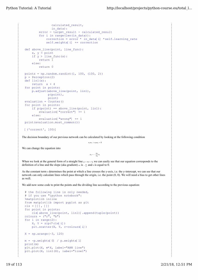
The decision boundary of our previous network can be calculated by looking at the following condition

We can change the equation into

When we look at the general form of a straight line , we can easily see that our equation corresponds to thedefinition of a line and the slope (aka gradient) is and is equal to 0.

As the constant term determines the point at which a line crosses the y-axis, i.e. the y-intercept, we can see that ournetwork can only calculate lines which pass through the origin, i.e. the point (0, 0). We will need a bias to get other linesas well.

We add now some code to print the points and the dividing line according to the previous equation:

# the following line is only needed,# if you use "ipython notebook":%matplotlib inline from matplotlib import pyplot as pltcls = [[], []]for point in points:

cls[above_line(point, lin1)].append(tuple(point))colours = ("r", "b")for i in range(2):

X, Y = zip(*cls[i])plt.scatter(X, Y, c=colours[i])

X = np.arange(-3, 120) m = -p.weights[0] / p.weights[1]print(m)plt.plot(X, m*X, label="ANN line")plt.plot(X, lin1(X), label="line1")

+ = 0x1w1 x2w2

= −x2w1

w2x1

y = mx+ b

m − w1

w2b

b


19 of 113 2/21/18, 12:51 PM

plt.legend()plt.show()

1.11082111934

We create a new dataset for our next experiments:

from matplotlib import pyplot as pltclass1 = [(3, 4), (4.2, 5.3), (4, 3), (6, 5), (4, 6), (3.7, 5.8),

(3.2, 4.6), (5.2, 5.9), (5, 4), (7, 4), (3, 7), (4.3, 4.3) ]class2 = [(-3, -4), (-2, -3.5), (-1, -6), (-3, -4.3), (-4, -5.6),

(-3.2, -4.8), (-2.3, -4.3), (-2.7, -2.6), (-1.5, -3.6),(-3.6, -5.6), (-4.5, -4.6), (-3.7, -5.8) ]

X, Y = zip(*class1)plt.scatter(X, Y, c="r")X, Y = zip(*class2)plt.scatter(X, Y, c="b")plt.show()

from itertools import chainp = Perceptron(2)def lin1(x):

return x + 4for point in class1:

p.adjust(1,p(point),point)

for point in class2:p.adjust(0,

p(point),point)

evaluation = Counter()for point in chain(class1, class2):

if p(point) == 1:evaluation["correct"] += 1



20 of 113 2/21/18, 12:51 PM

testpoints = [(3.9, 6.9), (-2.9, -5.9)]for point in testpoints:

print(p(point))

print(evaluation.most_common())

10[('correct', 12), ('wrong', 12)]

from matplotlib import pyplot as pltX, Y = zip(*class1)plt.scatter(X, Y, c="r")X, Y = zip(*class2)plt.scatter(X, Y, c="b")x = np.arange(-7, 10)y = 5*x + 10m = -p.weights[0] / p.weights[1]plt.plot(x, m*x)plt.show()

from matplotlib import pyplot as pltclass1 = [(3, 4, 3), (4.2, 5.3, 2.5), (4, 3, 3.8),

(6, 5, 2.7), (4, 6, 2.9), (3.7, 5.8, 4.2),(3.2, 4.6, 1.9), (5.2, 5.9, 2.7), (5, 4, 3.5),(7, 4, 2.7), (3, 7, 3.1), (4.3, 4.3, 3.8) ]

class2 = [(-3, -4, 7.6), (-2, -3.5, 6.9), (-1, -6, 8.6),(-3, -4.3, 7.4), (-4, -5.6, 7.9), (-3.2, -4.8, 5.3),(-2.3, -4.3, 8.1), (-2.7, -2.6, 7.3), (-1.5, -3.6, 7.8),(-3.6, -5.6, 6.8), (-4.5, -4.6, 8.3), (-3.7, -5.8, 8.7) ]

X, Y, Z = zip(*class1)plt.scatter(X, Y, Z, c="r")X, Y, Z = zip(*class2)plt.scatter(X, Y, Z, c="b")plt.show()


21 of 113 2/21/18, 12:51 PM

S I N G L E L AY E R W I T H B I A S

If two data clusters (classes) can be separated by a decision boundary in the form of a linear equation

they are called linearly separable.

Otherwise, i.e. if such a decision boundary does not exist, the two classes are called linearly inseparable. In this case, wecannot use a simple neural network.

For this purpose, we need neural networks with bias nodes, like the one in the following diagram:

Now, the linear equation for a perceptron contains a bias:

In the following section, we will introduce the XOR problem for neural networks. It is the simplest example of a nonlinearly separable neural network. I can be solved with an additional layer of neurons, which is called a hidden layer.

⋅ = 0∑i=1

n

xi wi

b+ ⋅ = 0∑i=1

n

xi wi


22 of 113 2/21/18, 12:51 PM

T H E X O R P R O B L E M F O R N E U R A L N E T W O R K S

The XOR (exclusive or) function is defined by the following truth table:

Input1 Input2 XOR Output

0 0 0

0 1 1

1 0 1

1 1 0

This problem can't be solved with a simple neural network. We need to introduce a new type of neural networks, anetwork with so-called hidden layers. A hidden layer allows the network to reorganize or rearrange the input data.

ANN with hidden layers:

The task is to find a line which separates the orange points from the blue points. But they can be separated by two lines,e.g. L1 and L2 in the following diagram:

To solve this problem, we need a network of the following kind, i.e with a hidden layer N1 and N2


23 of 113 2/21/18, 12:51 PM

The neuron N1 will determine one line, e.g. L1 and the neuron N2 will determine the other line L2. N3 will finally solveour problem:

NEURAL NETWORK WITH BIAS VALUES

We will come back now to our initial example with the random points above and below a line. We will rewrite the codeusing a bias value.


24 of 113 2/21/18, 12:51 PM

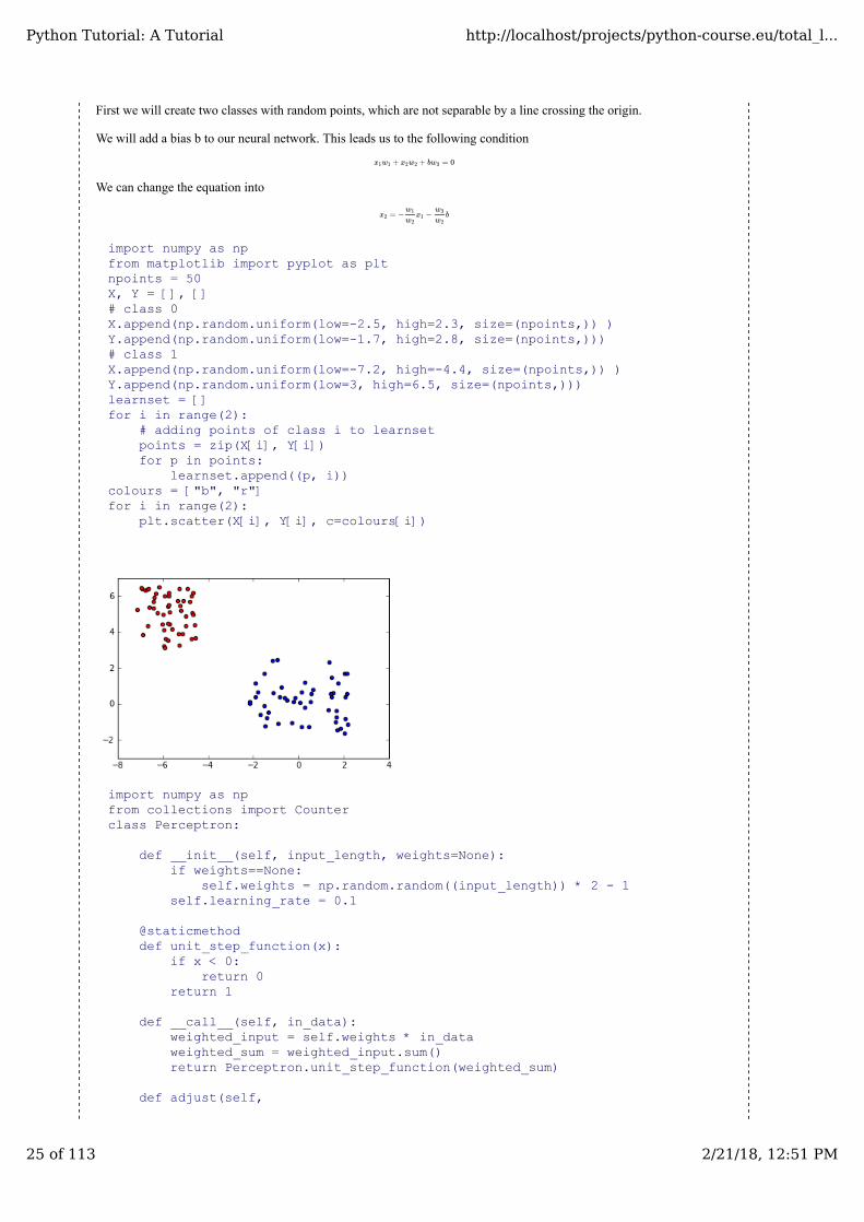
First we will create two classes with random points, which are not separable by a line crossing the origin.

We will add a bias b to our neural network. This leads us to the following condition

We can change the equation into

import numpy as npfrom matplotlib import pyplot as pltnpoints = 50X, Y = [], []# class 0X.append(np.random.uniform(low=-2.5, high=2.3, size=(npoints,)) )Y.append(np.random.uniform(low=-1.7, high=2.8, size=(npoints,)))# class 1X.append(np.random.uniform(low=-7.2, high=-4.4, size=(npoints,)) )Y.append(np.random.uniform(low=3, high=6.5, size=(npoints,)))learnset = []for i in range(2):

# adding points of class i to learnsetpoints = zip(X[i], Y[i])for p in points:

learnset.append((p, i))colours = ["b", "r"]for i in range(2):

plt.scatter(X[i], Y[i], c=colours[i])



self.weights = np.random.random((input_length)) * 2 - 1self.learning_rate = 0.1


if x < 0:return 0

return 1


def adjust(self,

+ + b = 0x1w1 x2w2 w3

= − − bx2w1

w2x1

w3

w2


25 of 113 2/21/18, 12:51 PM

target_result,calculated_result,in_data):


correction = error * in_data[i] *self.learning_rateself.weights[i] += correction

p = Perceptron(2)for point, label in learnset:

p.adjust(label,p(point),point)

evaluation = Counter()for point, label in learnset:

if p(point) == label:evaluation["correct"] += 1


print(evaluation.most_common())colours = ["b", "r"]for i in range(2):

plt.scatter(X[i], Y[i], c=colours[i])XR = np.arange(-8, 4) m = -p.weights[0] / p.weights[1]print(m)plt.plot(XR, m*XR, label="decision boundary")plt.legend()plt.show()

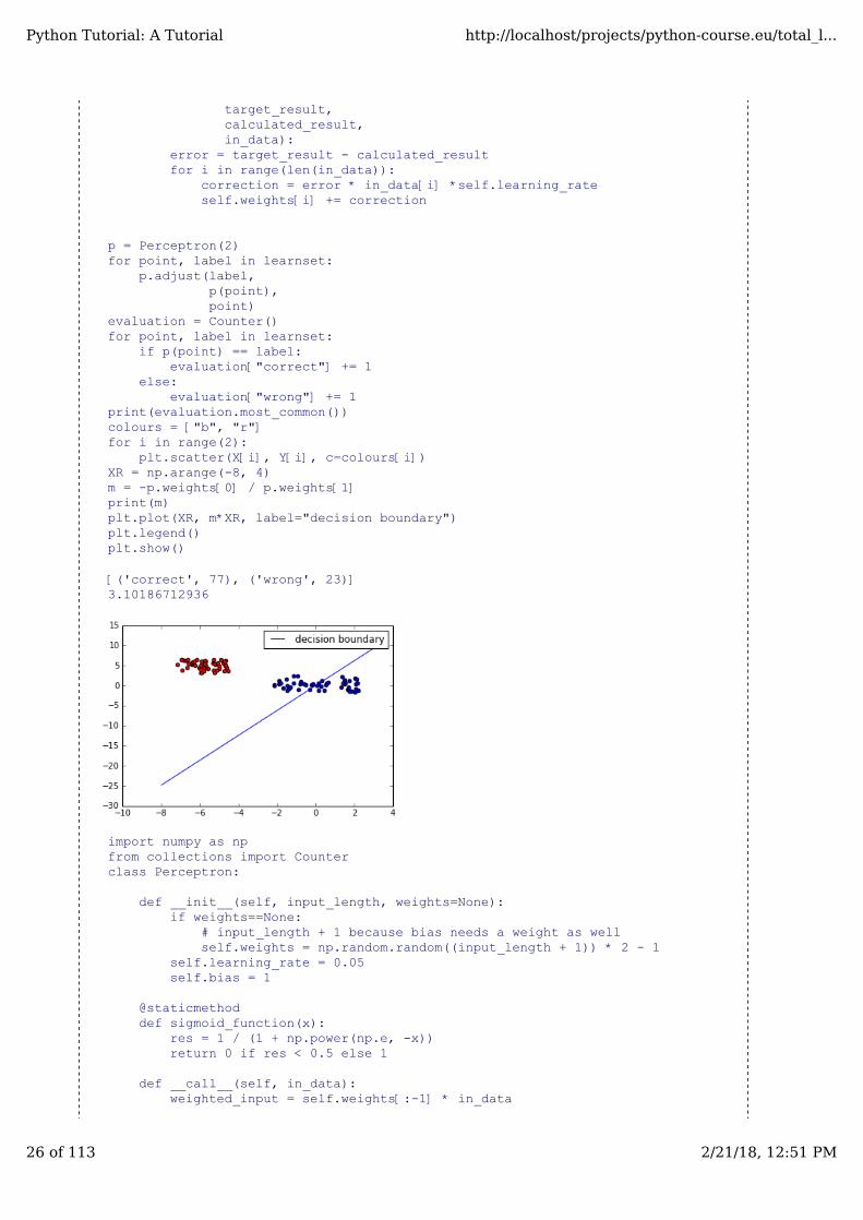
[('correct', 77), ('wrong', 23)]3.10186712936



# input_length + 1 because bias needs a weight as wellself.weights = np.random.random((input_length + 1)) * 2 - 1

self.learning_rate = 0.05self.bias = 1

@staticmethoddef sigmoid_function(x):

res = 1 / (1 + np.power(np.e, -x))return 0 if res < 0.5 else 1

def __call__(self, in_data):

weighted_input = self.weights[:-1] * in_data


26 of 113 2/21/18, 12:51 PM

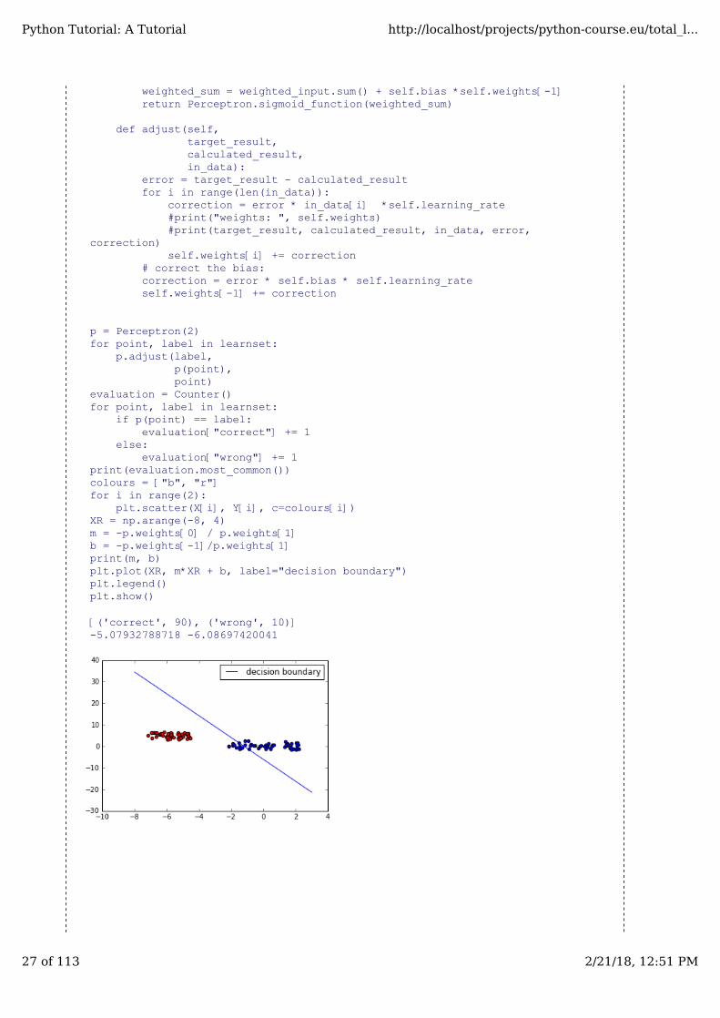
weighted_sum = weighted_input.sum() + self.bias *self.weights[-1]return Perceptron.sigmoid_function(weighted_sum)

def adjust(self,

target_result,calculated_result,in_data):


correction = error * in_data[i] *self.learning_rate#print("weights: ", self.weights)#print(target_result, calculated_result, in_data, error,

correction)self.weights[i] += correction

# correct the bias:correction = error * self.bias * self.learning_rateself.weights[-1] += correction

p = Perceptron(2)for point, label in learnset:

p.adjust(label,p(point),point)

evaluation = Counter()for point, label in learnset:

if p(point) == label:evaluation["correct"] += 1


print(evaluation.most_common())colours = ["b", "r"]for i in range(2):

plt.scatter(X[i], Y[i], c=colours[i])XR = np.arange(-8, 4) m = -p.weights[0] / p.weights[1]b = -p.weights[-1]/p.weights[1]print(m, b)plt.plot(XR, m*XR + b, label="decision boundary")plt.legend()plt.show()

[('correct', 90), ('wrong', 10)]-5.07932788718 -6.08697420041


27 of 113 2/21/18, 12:51 PM

We will need only one hidden layer with two neurons. One works like an AND gate and the other one like an OR gate.The output will "fire", when the OR gate fires and the AND gate doesn't.


28 of 113 2/21/18, 12:51 PM

N E U R O N A L N E T W O R K U S I N G P Y T H O N A N D N U M P Y

INTRODUCTION

We have introduced the basic ideas aboutneuronal networks in the previous chapterof our tutorial.

We pointed out the similarity betweenneurons and neural networks in biology.We also introduced very small articialneural networks and introduced decisionboundaries and the XOR problem.

The focus in our previous chapter had notbeen on efficiency.

We will introduce a Neural Network classin Python in this chapter, which will usethe powerful and efficient data structuresof Numpy. This way, we get a moreefficient network than in our previouschapter. When we say "more efficient", wedo not mean that the artificial neuralnetworks encountered in this chaper of ourtutorial are efficient and ready for real lifeusage. They are still quite slow comparedto implementations from sklearn forexample. The focus is to implement a very basic neural network and by doing this explaining the basic ideas. We want todemonstrate simple and easy to grasp networks.

Ideas like how the signal flow inside of a network works, how to implement weights. how to initialize weight matrices orwhat activation functions can be used.

We will start with a simple neural networks consisting of three layers, i.e. the input layer, a hidden layer and an outputlayer.

A SIMPLE ARTIFICIAL NEURAL NETWORK STRUCTURE

You can see a simple neural network structure in the following diagram. We have an input layer with three nodes These nodes get the corresponding input values . The middle or hidden layer has four nodes . The input ofthis layer stems from the input layer. We will discuss the mechanism soon. Finally, our output layer consists of the twonodes

We have to note that some would call this a two layer network, because they don't count the inputs as a layer.

, ,i1 i2 i3

, ,x1 x2 x3 , , ,h1 h2 h3 h4

,o1 o2


29 of 113 2/21/18, 12:51 PM

The input layer consists of the nodes , and . In principle the input is a one-dimensional vector, like (2, 4, 11). A one-dimensional vector is represented in numpy like this:

import numpy as npinput_vector = np.array([2, 4, 11])print(input_vector)

[ 2 4 11]

In the algorithm, which we will write later, we will have to transpose it into a column vector, i.e. a two-dimensional arraywith just one column:

import numpy as npinput_vector = np.array([2, 4, 11])input_vector = np.array(input_vector, ndmin=2).Tprint(input_vector, input_vector.shape)

[[ 2] [ 4] [11]] (3, 1)

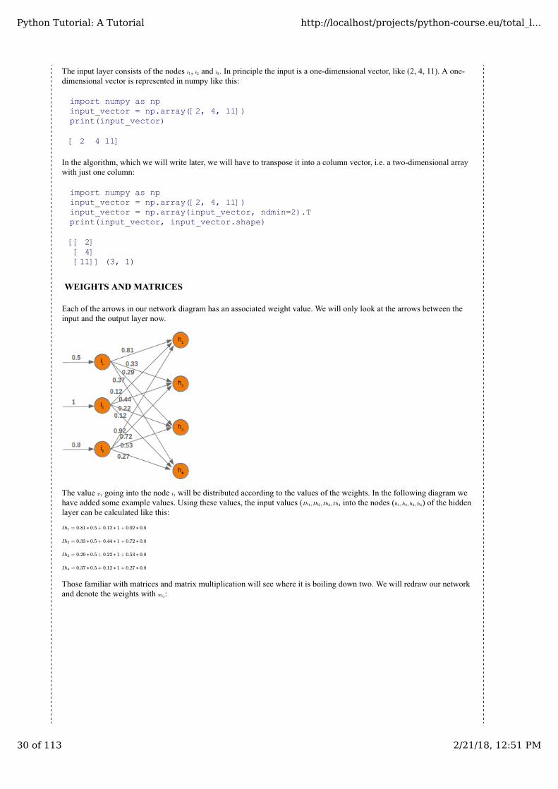
WEIGHTS AND MATRICES

Each of the arrows in our network diagram has an associated weight value. We will only look at the arrows between theinput and the output layer now.

The value going into the node will be distributed according to the values of the weights. In the following diagram wehave added some example values. Using these values, the input values ( into the nodes ( ) of the hiddenlayer can be calculated like this:

Those familiar with matrices and matrix multiplication will see where it is boiling down two. We will redraw our networkand denote the weights with :

i1 i2 i3

x1 i1

I , I , I , Ih1 h2 h3 h4 , , ,h1 h2 h3 h4

I = 0.81 ∗ 0.5 + 0.12 ∗ 1 + 0.92 ∗ 0.8h1

I = 0.33 ∗ 0.5 + 0.44 ∗ 1 + 0.72 ∗ 0.8h2

I = 0.29 ∗ 0.5 + 0.22 ∗ 1 + 0.53 ∗ 0.8h3

I = 0.37 ∗ 0.5 + 0.12 ∗ 1 + 0.27 ∗ 0.8h4

wij


30 of 113 2/21/18, 12:51 PM

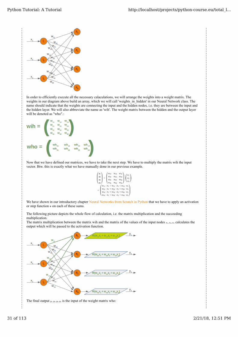
In order to efficiently execute all the necessary calaculations, we will arrange the weights into a weight matrix. Theweights in our diagram above build an array, which we will call 'weights_in_hidden' in our Neural Network class. Thename should indicate that the weights are connecting the input and the hidden nodes, i.e. they are between the input andthe hidden layer. We will also abbreviate the name as 'wih'. The weight matrix between the hidden and the output layerwill be denoted as "who".:

Now that we have defined our matrices, we have to take the next step. We have to multiply the matrix wih the inputvector. Btw. this is exactly what we have manually done in our previous example.

We have shown in our introductory chapter Neural Networks from Scratch in Python that we have to apply an activationor step function on each of these sums.

The following picture depicts the whole flow of calculation, i.e. the matrix multiplication and the succeedingmultiplication.The matrix multiplication between the matrix wih and the matrix of the values of the input nodes calculates theoutput which will be passed to the activation function.

The final output is the input of the weight matrix who:

=

⎛⎝⎜⎜⎜y1

y2

y3

y4

⎞⎠⎟⎟⎟

⎛⎝⎜⎜⎜w11

w21

w31

w41

w12

w22

w32

w42

w13

w23

w33

w43

⎞⎠⎟⎟⎟

⎛⎝⎜x1

x2

x3

⎞⎠⎟

=

⎛⎝⎜⎜⎜

⋅ + ⋅ + ⋅w11 x1 w12 x2 w13 x3

⋅ + ⋅ + ⋅w21 x1 w22 x2 w23 x3

⋅ + ⋅ + ⋅w31 x1 w32 x2 w33 x3

⋅ + ⋅ + ⋅w41 x1 w42 x2 w43 x3

⎞⎠⎟⎟⎟

Φ

, ,x1 x2 x3

, , ,y1 y2 y3 y4


31 of 113 2/21/18, 12:51 PM

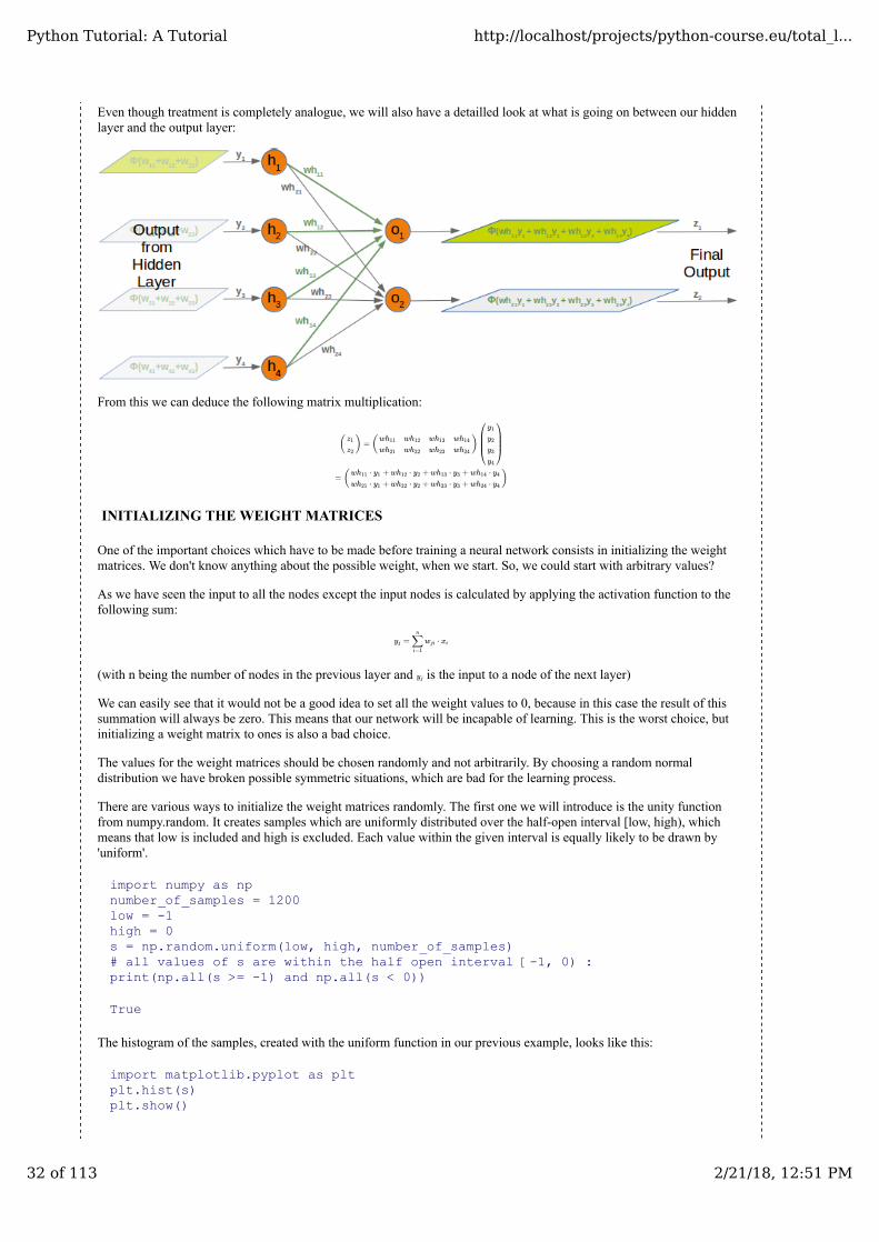
Even though treatment is completely analogue, we will also have a detailled look at what is going on between our hiddenlayer and the output layer:

From this we can deduce the following matrix multiplication:

INITIALIZING THE WEIGHT MATRICES

One of the important choices which have to be made before training a neural network consists in initializing the weightmatrices. We don't know anything about the possible weight, when we start. So, we could start with arbitrary values?

As we have seen the input to all the nodes except the input nodes is calculated by applying the activation function to thefollowing sum:

(with n being the number of nodes in the previous layer and is the input to a node of the next layer)

We can easily see that it would not be a good idea to set all the weight values to 0, because in this case the result of thissummation will always be zero. This means that our network will be incapable of learning. This is the worst choice, butinitializing a weight matrix to ones is also a bad choice.

The values for the weight matrices should be chosen randomly and not arbitrarily. By choosing a random normaldistribution we have broken possible symmetric situations, which are bad for the learning process.

There are various ways to initialize the weight matrices randomly. The first one we will introduce is the unity functionfrom numpy.random. It creates samples which are uniformly distributed over the half-open interval [low, high), whichmeans that low is included and high is excluded. Each value within the given interval is equally likely to be drawn by'uniform'.

import numpy as npnumber_of_samples = 1200low = -1high = 0s = np.random.uniform(low, high, number_of_samples)# all values of s are within the half open interval [-1, 0) :print(np.all(s >= -1) and np.all(s < 0))

True

The histogram of the samples, created with the uniform function in our previous example, looks like this:

import matplotlib.pyplot as pltplt.hist(s)plt.show()

( ) = ( )z1

z2

wh11

wh21

wh12

wh22

wh13

wh23

wh14

wh24

⎛⎝⎜⎜⎜y1

y2

y3

y4

⎞⎠⎟⎟⎟

= ( )w ⋅ + w ⋅ + w ⋅ + w ⋅h11 y1 h12 y2 h13 y3 h14 y4

w ⋅ + w ⋅ + w ⋅ + w ⋅h21 y1 h22 y2 h23 y3 h24 y4

= ⋅yj ∑i=1

n

wji xi

yj


32 of 113 2/21/18, 12:51 PM

The next function we will look at is 'binomial' from numpy.binomial:

binomial(n, p, size=None)

It draws samples from a binomial distribution with specified parameters, n trials and p probability of success where n is aninteger >= 0 and p is a float in the interval [0,1]. (n may be input as a float, but it is truncated to an integer in use)

s = np.random.binomial(100, 0.5, 1200)plt.hist(s)plt.show()

We like to create random numbers with a normal distribution, but the numbers have to be bounded. This is not the casewith np.random.normal(), because it doesn't offer any bound parameter.

We can use truncnorm from scipy.stats for this purpose.

The standard form of this distribution is a standard normal truncated to the range [a, b] — notice that a and b are definedover the domain of the standard normal. To convert clip values for a specific mean and standard deviation, use:

a, b = (myclip_a - my_mean) / my_std, (myclip_b - my_mean) / my_std

from scipy.stats import truncnorms = truncnorm(a=-2/3., b=2/3., scale=1, loc=0).rvs(size=1000)plt.hist(s)plt.show()


33 of 113 2/21/18, 12:51 PM

The function 'truncnorm' is difficult to use. To make life easier, we define a function 'truncated_normal' in the following tofascilitate this task:

def truncated_normal(mean=0, sd=1, low=0, upp=10):return truncnorm(

(low - mean) / sd, (upp - mean) / sd, loc=mean, scale=sd)X = truncated_normal(mean=0, sd=0.4, low=-0.5, upp=0.5)s = X.rvs(10000)plt.hist(s)plt.show()

Further examples:

X1 = truncated_normal(mean=2, sd=1, low=1, upp=10)X2 = truncated_normal(mean=5.5, sd=1, low=1, upp=10)X3 = truncated_normal(mean=8, sd=1, low=1, upp=10)import matplotlib.pyplot as pltfig, ax = plt.subplots(3, sharex=True)ax[0].hist(X1.rvs(10000), normed=True)ax[1].hist(X2.rvs(10000), normed=True)ax[2].hist(X3.rvs(10000), normed=True)plt.show()

We will create the link weights matrix now. 'truncated_normal' is ideal for this purpose. It is a good idea to choose random


34 of 113 2/21/18, 12:51 PM

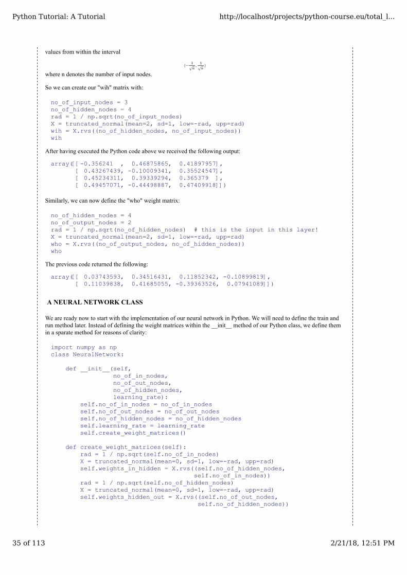
values from within the interval

where n denotes the number of input nodes.

So we can create our "wih" matrix with:

no_of_input_nodes = 3no_of_hidden_nodes = 4rad = 1 / np.sqrt(no_of_input_nodes)X = truncated_normal(mean=2, sd=1, low=-rad, upp=rad)wih = X.rvs((no_of_hidden_nodes, no_of_input_nodes))wih


array([[-0.356241 , 0.46875865, 0.41897957], [ 0.43267439, -0.10009341, 0.35524547], [ 0.45234311, 0.39339294, 0.365379 ], [ 0.49457071, -0.44498887, 0.47409918]])

Similarly, we can now define the "who" weight matrix:

no_of_hidden_nodes = 4no_of_output_nodes = 2rad = 1 / np.sqrt(no_of_hidden_nodes) # this is the input in this layer!X = truncated_normal(mean=2, sd=1, low=-rad, upp=rad)who = X.rvs((no_of_output_nodes, no_of_hidden_nodes))who

The previous code returned the following:

array([[ 0.03743593, 0.34516431, 0.11852342, -0.10899819], [ 0.11039838, 0.41685055, -0.39363526, 0.07941089]])

A NEURAL NETWORK CLASS

We are ready now to start with the implementation of our neural network in Python. We will need to define the train andrun method later. Instead of defining the weight matrices within the __init__ method of our Python class, we define themin a sparate method for reasons of clarity:

import numpy as npclass NeuralNetwork:

def __init__(self,no_of_in_nodes,no_of_out_nodes,no_of_hidden_nodes,learning_rate):

self.no_of_in_nodes = no_of_in_nodesself.no_of_out_nodes = no_of_out_nodesself.no_of_hidden_nodes = no_of_hidden_nodesself.learning_rate = learning_rate self.create_weight_matrices()

def create_weight_matrices(self):

rad = 1 / np.sqrt(self.no_of_in_nodes)X = truncated_normal(mean=0, sd=1, low=-rad, upp=rad)self.weights_in_hidden = X.rvs((self.no_of_hidden_nodes,

self.no_of_in_nodes))rad = 1 / np.sqrt(self.no_of_hidden_nodes)X = truncated_normal(mean=0, sd=1, low=-rad, upp=rad)self.weights_hidden_out = X.rvs((self.no_of_out_nodes,

self.no_of_hidden_nodes))

(− , )1n−−√

1n−−√


35 of 113 2/21/18, 12:51 PM

def train(self):pass

def run(self):

pass if __name__ == "__main__":

simple_network = NeuralNetwork(no_of_in_nodes = 3,no_of_out_nodes = 2,no_of_hidden_nodes = 4,learning_rate = 0.1)

print(simple_network.weights_in_hidden)print(simple_network.weights_hidden_out)

[[ 0.10607641 -0.05716482 0.55752363] [ 0.33701589 0.05461437 0.5521666 ] [ 0.11990863 -0.29320233 -0.43600856] [-0.18218775 -0.20794852 -0.39419628]][[ 4.82634085e-04 -4.97611184e-01 -3.25708215e-01 -2.61086173e-01] [ -2.04995922e-01 -7.08439635e-02 2.66347839e-01 4.87601670e-01]]

ACTIVATION FUNCTIONS, SIGMOID AND RELU

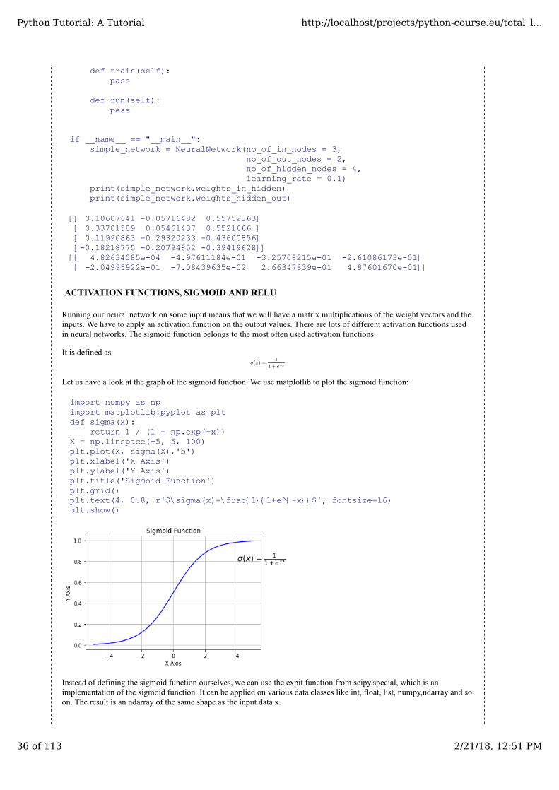
Running our neural network on some input means that we will have a matrix multiplications of the weight vectors and theinputs. We have to apply an activation function on the output values. There are lots of different activation functions usedin neural networks. The sigmoid function belongs to the most often used activation functions.

It is defined as

Let us have a look at the graph of the sigmoid function. We use matplotlib to plot the sigmoid function:

import numpy as npimport matplotlib.pyplot as pltdef sigma(x):

return 1 / (1 + np.exp(-x))X = np.linspace(-5, 5, 100)plt.plot(X, sigma(X),'b')plt.xlabel('X Axis')plt.ylabel('Y Axis')plt.title('Sigmoid Function')plt.grid()plt.text(4, 0.8, r'$\sigma(x)=\frac{1}{1+e^{-x}}$', fontsize=16)plt.show()

Instead of defining the sigmoid function ourselves, we can use the expit function from scipy.special, which is animplementation of the sigmoid function. It can be applied on various data classes like int, float, list, numpy,ndarray and soon. The result is an ndarray of the same shape as the input data x.

σ(x) =1

1 + e−x


36 of 113 2/21/18, 12:51 PM

from scipy.special import expitprint(expit(3.4))print(expit([3, 4, 1]))print(expit(np.array([0.8, 2.3, 8])))

0.967704535302[ 0.95257413 0.98201379 0.73105858][ 0.68997448 0.90887704 0.99966465]

ADDING A RUN METHOD

We can use this as the activation function of our neural network. As you most probably know, we can directly assign anew name, when we import the function:

from scipy.special import expit as activation_function

import numpy as npfrom scipy.special import expit as activation_functionfrom scipy.stats import truncnormdef truncated_normal(mean=0, sd=1, low=0, upp=10):

return truncnorm((low - mean) / sd, (upp - mean) / sd, loc=mean, scale=sd)

class NeuralNetwork:


self.no_of_in_nodes = no_of_in_nodesself.no_of_out_nodes = no_of_out_nodesself.no_of_hidden_nodes = no_of_hidden_nodesself.learning_rate = learning_rateself.create_weight_matrices()


""" A method to initialize the weight matrices of the neural network"""




def train(self, input_vector, target_vector):pass

def run(self, input_vector):"""

running the network with an input vector input_vector. input_vector can be tuple, list or ndarray """

# turning the input vector into a column vectorinput_vector = np.array(input_vector, ndmin=2).Toutput_vector = np.dot(self.weights_in_hidden, input_vector)output_vector = activation_function(output_vector)

output_vector = np.dot(self.weights_hidden_out, output_vector)output_vector = activation_function(output_vector)


37 of 113 2/21/18, 12:51 PM

return output_vector

There is still a train method missing. We can instantiate and run this network, but the results will not make sense. They arebased on the random weight matrices:

simple_network = NeuralNetwork(no_of_in_nodes=2,no_of_out_nodes=2,no_of_hidden_nodes=10,learning_rate=0.6)

simple_network.run([(3, 4)])


array([[ 0.66413143], [ 0.45385657]])

We can also define our own sigmoid function with the decorator vectorize from numpy:

@np.vectorizedef sigmoid(x):

return 1 / (1 + np.e ** -x)#sigmoid = np.vectorize(sigmoid)sigmoid([3, 4, 5])


array([ 0.95257413, 0.98201379, 0.99330715])

We add training support in our next class definition, i.e. we define the method 'train':

import numpy as [email protected] sigmoid(x):

return 1 / (1 + np.e ** -x)activation_function = sigmoidfrom scipy.stats import truncnormdef truncated_normal(mean=0, sd=1, low=0, upp=10):











38 of 113 2/21/18, 12:51 PM

def train(self, input_vector, target_vector):

# input_vector and target_vector can be tuple, list or ndarray

input_vector = np.array(input_vector, ndmin=2).Ttarget_vector = np.array(target_vector, ndmin=2).T

output_vector1 = np.dot(self.weights_in_hidden, input_vector)output_vector_hidden = activation_function(output_vector1)

output_vector2 = np.dot(self.weights_hidden_out, output_vector_hidden)output_vector_network = activation_function(output_vector2)

output_errors = target_vector - output_vector_network# update the weights:tmp = output_errors * output_vector_network * (1.0 -

output_vector_network) tmp = self.learning_rate * np.dot(tmp, output_vector_hidden.T)self.weights_hidden_out += tmp# calculate hidden errors:hidden_errors = np.dot(self.weights_hidden_out.T, output_errors)# update the weights:tmp = hidden_errors * output_vector_hidden * (1.0 -

output_vector_hidden)self.weights_in_hidden += self.learning_rate * np.dot(tmp,

input_vector.T)

def run(self, input_vector):# input_vector can be tuple, list or ndarrayinput_vector = np.array(input_vector, ndmin=2).Toutput_vector = np.dot(self.weights_in_hidden, input_vector)output_vector = activation_function(output_vector)



We will test our network with the same example, we created in the chapter [Neural Networks from Scratch](neural_networks.php):

import numpy as npfrom matplotlib import pyplot as pltdata1 = [((3, 4), (0.99, 0.01)), ((4.2, 5.3), (0.99, 0.01)),

((4, 3), (0.99, 0.01)), ((6, 5), (0.99, 0.01)),((4, 6), (0.99, 0.01)), ((3.7, 5.8), (0.99, 0.01)),((3.2, 4.6), (0.99, 0.01)), ((5.2, 5.9), (0.99, 0.01)),((5, 4), (0.99, 0.01)), ((7, 4), (0.99, 0.01)),((3, 7), (0.99, 0.01)), ((4.3, 4.3), (0.99, 0.01))]

data2 = [((-3, -4), (0.01, 0.99)), ((-2, -3.5), (0.01, 0.99)),((-1, -6), (0.01, 0.99)), ((-3, -4.3), (0.01, 0.99)),((-4, -5.6), (0.01, 0.99)), ((-3.2, -4.8), (0.01, 0.99)),((-2.3, -4.3), (0.01, 0.99)), ((-2.7, -2.6), (0.01, 0.99)),((-1.5, -3.6), (0.01, 0.99)), ((-3.6, -5.6), (0.01, 0.99)),((-4.5, -4.6), (0.01, 0.99)), ((-3.7, -5.8), (0.01, 0.99))]

data = data1 + data2np.random.shuffle(data)points1, labels1 = zip(*data1)X, Y = zip(*points1)plt.scatter(X, Y, c="r")points2, labels2 = zip(*data2)X, Y = zip(*points2)plt.scatter(X, Y, c="b")plt.show()


39 of 113 2/21/18, 12:51 PM

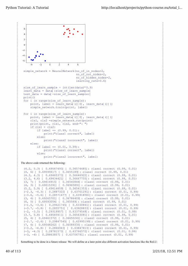
simple_network = NeuralNetwork(no_of_in_nodes=2,no_of_out_nodes=2,no_of_hidden_nodes=2,learning_rate=0.6)

size_of_learn_sample = int(len(data)*0.9)learn_data = data[:size_of_learn_sample]test_data = data[-size_of_learn_sample:]print()for i in range(size_of_learn_sample):

point, label = learn_data[i][0], learn_data[i][1]simple_network.train(point, label)

for i in range(size_of_learn_sample):

point, label = learn_data[i][0], learn_data[i][1]cls1, cls2 =simple_network.run(point)print(point, cls1, cls2, end=": ")if cls1 > cls2:

if label == (0.99, 0.01):print("class1 correct", label)

else:print("class2 incorrect", label)

else:if label == (0.01, 0.99):

print("class1 correct", label)else:

print("class2 incorrect", label)

The above code returned the following:

(4.2, 5.3) [ 0.69567493] [ 0.36574485]: class1 correct (0.99, 0.01)(4, 6) [ 0.69599417] [ 0.3655189]: class1 correct (0.99, 0.01)(4.3, 4.3) [ 0.69465373] [ 0.36646922]: class1 correct (0.99, 0.01)(3.2, 4.6) [ 0.69434421] [ 0.36667755]: class1 correct (0.99, 0.01)(3, 7) [ 0.69614915] [ 0.36540844]: class1 correct (0.99, 0.01)(4, 3) [ 0.69015391] [ 0.36965891]: class1 correct (0.99, 0.01)(5.2, 5.9) [ 0.69614659] [ 0.36541353]: class1 correct (0.99, 0.01)(-2.3, -4.3) [ 0.2887322] [ 0.63701291]: class1 correct (0.01, 0.99)(-3.6, -5.6) [ 0.28571677] [ 0.63918581]: class1 correct (0.01, 0.99)(3, 4) [ 0.69265701] [ 0.36786409]: class1 correct (0.99, 0.01)(6, 5) [ 0.69593054] [ 0.365569]: class1 correct (0.99, 0.01)(-1.5, -3.6) [ 0.29421745] [ 0.6330841]: class1 correct (0.01, 0.99)(-3.7, -5.8) [ 0.2855751] [ 0.63928833]: class1 correct (0.01, 0.99)(-2, -3.5) [ 0.29319957] [ 0.63379548]: class1 correct (0.01, 0.99)(3.7, 5.8) [ 0.69583411] [ 0.36563081]: class1 correct (0.99, 0.01)(5, 4) [ 0.69461572] [ 0.36650241]: class1 correct (0.99, 0.01)(-2.7, -2.6) [ 0.29847545] [ 0.62995199]: class1 correct (0.01, 0.99)(7, 4) [ 0.69548262] [ 0.36589335]: class1 correct (0.99, 0.01)(-3.2, -4.8) [ 0.2866943] [ 0.63847813]: class1 correct (0.01, 0.99)(-3, -4.3) [ 0.28781573] [ 0.63766572]: class1 correct (0.01, 0.99)(-3, -4) [ 0.28863857] [ 0.63706791]: class1 correct (0.01, 0.99)

Something to be done in a future release: We will define at a later point also different activation functions like the ReLU:


40 of 113 2/21/18, 12:51 PM

# alternative activation functiondef ReLU(x):

return np.maximum(0.0, x)# derivation of reludef ReLU_derivation(x):

if x <= 0:return 0

else:return 1

import numpy as npimport matplotlib.pyplot as pltX = np.linspace(-5, 5, 100)plt.plot(X, ReLU(X),'b')plt.xlabel('X Axis')plt.ylabel('Y Axis')plt.title('ReLU Function')plt.grid()plt.text(3, 0.8, r'$ReLU(x)=max(0.0, x)$', fontsize=16)plt.show()

NEURAL NETWORK WITH BIAS NODES

A bias node is a node that is always returning the same output. In other words: It is a node which is not depending onsome input and it does not have any input. The value of a bias node is often set to one, but it can be other values as well.Except 0 which doesn't make sense. If a neural network does not have a bias node in a given layer, it will not be able toproduce output in the next layer that differs from 0 when the feature values are 0. Generally speaking, we can say that biasnodes are used to increase the flexibility of the network to fit the data. Usually, there will be not more than one bias nodeper layer. The only exception is the output layer, because it makes no sense to add a bias node to this layer.

We can see from this diagram that our weight matrix will have one more column and the bias value is added to the input


41 of 113 2/21/18, 12:51 PM

vector:

Again, the situation for the weight matrix between the hidden and the outputlayer is similar:

The same is true for the corresponding matrix:

The following is a complete Python class implementing our network with bias nodes:





def __init__(self,no_of_in_nodes,no_of_out_nodes,no_of_hidden_nodes,learning_rate,bias=None):

self.no_of_in_nodes = no_of_in_nodesself.no_of_out_nodes = no_of_out_nodes

self.no_of_hidden_nodes = no_of_hidden_nodes

self.learning_rate = learning_rateself.bias = biasself.create_weight_matrices()


42 of 113 2/21/18, 12:51 PM

def create_weight_matrices(self):""" A method to initialize the weight matrices of the neural

network with optional bias nodes"""

bias_node = 1 if self.bias else 0

rad = 1 / np.sqrt(self.no_of_in_nodes + bias_node)X = truncated_normal(mean=0, sd=1, low=-rad, upp=rad)self.weights_in_hidden = X.rvs((self.no_of_hidden_nodes,

self.no_of_in_nodes + bias_node))rad = 1 / np.sqrt(self.no_of_hidden_nodes + bias_node)X = truncated_normal(mean=0, sd=1, low=-rad, upp=rad)self.weights_hidden_out = X.rvs((self.no_of_out_nodes,

self.no_of_hidden_nodes + bias_node))

def train(self, input_vector, target_vector):# input_vector and target_vector can be tuple, list or ndarray

bias_node = 1 if self.bias else 0if self.bias:

# adding bias node to the end of the inpuy_vectorinput_vector = np.concatenate( (input_vector, [self.bias]) )


output_vector1 = np.dot(self.weights_in_hidden, input_vector)output_vector_hidden = activation_function(output_vector1)

if self.bias:

output_vector_hidden = np.concatenate( (output_vector_hidden,[[self.bias]]) )

output_vector2 = np.dot(self.weights_hidden_out, output_vector_hidden)output_vector_network = activation_function(output_vector2)


output_vector_network) tmp = self.learning_rate * np.dot(tmp, output_vector_hidden.T)self.weights_hidden_out += tmp# calculate hidden errors:hidden_errors = np.dot(self.weights_hidden_out.T, output_errors)# update the weights:tmp = hidden_errors * output_vector_hidden * (1.0 -

output_vector_hidden)if self.bias:

x = np.dot(tmp, input_vector.T)[:-1,:] # ???? last element cut off, ???

else:x = np.dot(tmp, input_vector.T)

self.weights_in_hidden += self.learning_rate * x

def run(self, input_vector):# input_vector can be tuple, list or ndarray


43 of 113 2/21/18, 12:51 PM

if self.bias:# adding bias node to the end of the inpuy_vectorinput_vector = np.concatenate( (input_vector, [1]) )

input_vector = np.array(input_vector, ndmin=2).Toutput_vector = np.dot(self.weights_in_hidden, input_vector)output_vector = activation_function(output_vector)

if self.bias:

output_vector = np.concatenate( (output_vector, [[1]]) )



class1 = [(3, 4), (4.2, 5.3), (4, 3), (6, 5), (4, 6), (3.7, 5.8),(3.2, 4.6), (5.2, 5.9), (5, 4), (7, 4), (3, 7), (4.3, 4.3) ]

class2 = [(-3, -4), (-2, -3.5), (-1, -6), (-3, -4.3), (-4, -5.6),(-3.2, -4.8), (-2.3, -4.3), (-2.7, -2.6), (-1.5, -3.6),(-3.6, -5.6), (-4.5, -4.6), (-3.7, -5.8) ]

labeled_data = []for el in class1:

labeled_data.append( [el, [1, 0]])for el in class2:

labeled_data.append([el, [0, 1]]) np.random.shuffle(labeled_data)print(labeled_data[:10])data, labels = zip(*labeled_data)labels = np.array(labels)data = np.array(data)

[[(-1, -6), [0, 1]], [(-2.3, -4.3), [0, 1]], [(-3, -4), [0, 1]], [(-2, -3.5), [0, 1]], [(3.2, 4.6), [1, 0]], [(-3.7, -5.8), [0, 1]], [(4, 3), [1, 0]], [(4, 6), [1, 0]], [(3.7, 5.8), [1, 0]], [(5.2, 5.9), [1, 0]]]

simple_network = NeuralNetwork(no_of_in_nodes=2,no_of_out_nodes=2,no_of_hidden_nodes=10,learning_rate=0.1,bias=None)

for _ in range(20):

for i in range(len(data)):simple_network.train(data[i], labels[i])

for i in range(len(data)):print(labels[i])print(simple_network.run(data[i]))

[0 1][[ 0.06857234] [ 0.93333256]][0 1][[ 0.0694426 ] [ 0.93263667]][0 1][[ 0.06890567] [ 0.93314354]][0 1][[ 0.07398586] [ 0.92826171]][1 0][[ 0.91353761]


44 of 113 2/21/18, 12:51 PM

[ 0.08620027]][0 1][[ 0.06598966] [ 0.93595685]][1 0][[ 0.90963169] [ 0.09022392]][1 0][[ 0.9155282 ] [ 0.08423438]][1 0][[ 0.91531178] [ 0.08444738]][1 0][[ 0.91575254] [ 0.08401871]][1 0][[ 0.91164767] [ 0.08807266]][0 1][[ 0.06818507] [ 0.93384242]][0 1][[ 0.07609557] [ 0.92620649]][0 1][[ 0.06651258] [ 0.93543384]][1 0][[ 0.91411049] [ 0.08570024]][1 0][[ 0.91409934] [ 0.08567811]][0 1][[ 0.06711438] [ 0.93487441]][1 0][[ 0.91517701] [ 0.08458689]][1 0][[ 0.91550873] [ 0.08427926]][1 0][[ 0.91562321] [ 0.08414424]][0 1][[ 0.06613625] [ 0.93581576]][0 1][[ 0.0659944] [ 0.9359505]][0 1][[ 0.07744433] [ 0.92481335]][1 0][[ 0.91498511] [ 0.08485322]]


45 of 113 2/21/18, 12:51 PM

N E U R A L N E T W O R K

TESTING WITH MNIST

The MNIST database (Modified National Institute ofStandards and Technology database) of handwrittendigits consists of a training set of 60,000 examples, anda test set of 10,000 examples. It is a subset of a largerset available from NIST. Additionally, the black andwhite images from NIST were size-normalized andcentered to fit into a 28x28 pixel bounding box andanti-aliased, which introduced grayscale levels.

This database is well liked for training and testing inthe field of machine learning and image processing. Itis a remixed subset of the original NIST datasets. Onehalf of the 60,000 training images consist of imagesfrom NIST's testing dataset and the other half fromNist's training set. The 10,000 images from the testingset are similarly assembled.

The MNIST dataset is used by researchers to test andcompare their research results with others. The lowesterror rates in literature are as low as 0.21 percent.1

READING THE MNIST DATA SET

The images from the data set have the size 28 x 28. They are saved in the csv data files mnist_train.csv and mnist_test.csv.

Every line of these files consists of an image, i.e. 785 numbers between 0 and 255.

The first number of each line is the label, i.e. the digit which is depicted in the image. The following 784 numbers are thepixels of the 28 x 28 image.

%matplotlib inlineimport numpy as npimport matplotlib.pyplot as pltimage_size = 28 # width and lengthno_of_different_labels = 10 # i.e. 0, 1, 2, 3, ..., 9image_pixels = image_size * image_sizedata_path = "data/mnist/"train_data = np.loadtxt(data_path + "mnist_train.csv",

delimiter=",")test_data = np.loadtxt(data_path + "mnist_test.csv",

delimiter=",")

We map the values of the image data into the interval [0.01, 0.99] by dividing the train_data and test_data arrays by (255 *0.99 + 0.01)

This way, we have input values between 0 and 1 but not including 0 and 1.

fac = 255 *0.99 + 0.01train_imgs = np.asfarray(train_data[:, 1:]) / factest_imgs = np.asfarray(test_data[:, 1:]) / factrain_labels = np.asfarray(train_data[:, :1])test_labels = np.asfarray(test_data[:, :1])

We need the labels in our calculations in a one-hot representation. We have 10 digits from 0 to 9, i.e. lr = np.arange(10).


46 of 113 2/21/18, 12:51 PM

Turning a label into one-hot representation can be achieved with the command: (lr==label).astype(np.int)

We demonstrate this in the following:

import numpy as nplr = np.arange(10)for label in range(10):

one_hot = (lr==label).astype(np.int)print("label: ", label, " in one-hot representation: ", one_hot)

label: 0 in one-hot representation: [1 0 0 0 0 0 0 0 0 0]label: 1 in one-hot representation: [0 1 0 0 0 0 0 0 0 0]label: 2 in one-hot representation: [0 0 1 0 0 0 0 0 0 0]label: 3 in one-hot representation: [0 0 0 1 0 0 0 0 0 0]label: 4 in one-hot representation: [0 0 0 0 1 0 0 0 0 0]label: 5 in one-hot representation: [0 0 0 0 0 1 0 0 0 0]label: 6 in one-hot representation: [0 0 0 0 0 0 1 0 0 0]label: 7 in one-hot representation: [0 0 0 0 0 0 0 1 0 0]label: 8 in one-hot representation: [0 0 0 0 0 0 0 0 1 0]label: 9 in one-hot representation: [0 0 0 0 0 0 0 0 0 1]

We are ready now to turn our labelled images into one-hot representations. Instead of zeroes and one, we create 0.01 and0.99, which will be better for our calculations:

lr = np.arange(no_of_different_labels)# transform labels into one hot representationtrain_labels_one_hot = (lr==train_labels).astype(np.float)test_labels_one_hot = (lr==test_labels).astype(np.float)# we don't want zeroes and ones in the labels neither:train_labels_one_hot[train_labels_one_hot==0] = 0.01train_labels_one_hot[train_labels_one_hot==1] = 0.99test_labels_one_hot[test_labels_one_hot==0] = 0.01test_labels_one_hot[test_labels_one_hot==1] = 0.99

Before we start using the MNIST data sets with our neural network, we will have a look at same images:

for i in range(10):img = train_imgs[i].reshape((28,28))plt.imshow(img, cmap="Greys")plt.show()


47 of 113 2/21/18, 12:51 PM

DUMPING THE DATA FOR FASTER RELOAD

You may have noticed that it is quite slow to read in the data from the csv files.

We will save the data in binary format with the dump function from the pickle module:

import picklewith open("data/mnist/pickled_mnist.pkl", "bw") as fh:

data = (train_imgs,test_imgs,train_labels,test_labels,train_labels_one_hot,test_labels_one_hot)

pickle.dump(data, fh)

We are able now to read in the data by using pickle.load. This is a lot faster than using loadtxt on the csv files:

import picklewith open("data/mnist/pickled_mnist.pkl", "br") as fh:


48 of 113 2/21/18, 12:51 PM

data = pickle.load(fh)train_imgs = data[0]test_imgs = data[1]train_labels = data[2]test_labels = data[3]train_labels_one_hot = data[4]test_labels_one_hot = data[5]image_size = 28 # width and lengthno_of_different_labels = 10 # i.e. 0, 1, 2, 3, ..., 9image_pixels = image_size * image_size

CLASSIFYING THE DATA

We will use the following neuronal network class for our first classification:



return truncnorm((low - mean) / sd,(upp - mean) / sd,loc=mean,scale=sd)





""" A method to initialize the weight matrices of the neural network """

rad = 1 / np.sqrt(self.no_of_in_nodes)X = truncated_normal(mean=0,

sd=1,low=-rad,upp=rad)

self.wih = X.rvs((self.no_of_hidden_nodes,self.no_of_in_nodes))

rad = 1 / np.sqrt(self.no_of_hidden_nodes)X = truncated_normal(mean=0, sd=1, low=-rad, upp=rad)self.who = X.rvs((self.no_of_out_nodes,


def train(self, input_vector, target_vector):"""

input_vector and target_vector can be tuple, list or ndarray """


49 of 113 2/21/18, 12:51 PM


output_vector1 = np.dot(self.wih,

input_vector)output_hidden = activation_function(output_vector1)

output_vector2 = np.dot(self.who,

output_hidden)output_network = activation_function(output_vector2)

output_errors = target_vector - output_network# update the weights:tmp = output_errors * output_network \

* (1.0 - output_network) tmp = self.learning_rate * np.dot(tmp,

output_hidden.T)self.who += tmp# calculate hidden errors:hidden_errors = np.dot(self.who.T,

output_errors)# update the weights:tmp = hidden_errors * output_hidden * \

(1.0 - output_hidden)self.wih += self.learning_rate \

* np.dot(tmp, input_vector.T)

def run(self, input_vector):# input_vector can be tuple, list or ndarrayinput_vector = np.array(input_vector, ndmin=2).Toutput_vector = np.dot(self.wih,

input_vector)output_vector = activation_function(output_vector)

output_vector = np.dot(self.who,

output_vector)output_vector = activation_function(output_vector)


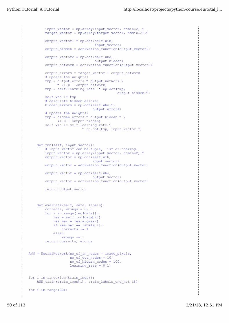
def evaluate(self, data, labels):corrects, wrongs = 0, 0for i in range(len(data)):

res = self.run(data[i])res_max = res.argmax()if res_max == labels[i]:

corrects += 1else:

wrongs += 1return corrects, wrongs

ANN = NeuralNetwork(no_of_in_nodes = image_pixels,no_of_out_nodes = 10,no_of_hidden_nodes = 100,learning_rate = 0.1)

for i in range(len(train_imgs)):

ANN.train(train_imgs[i], train_labels_one_hot[i])

for i in range(20):


50 of 113 2/21/18, 12:51 PM

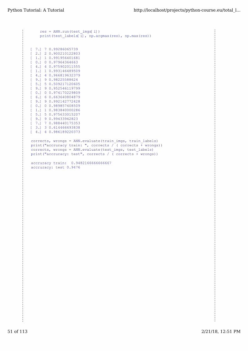
res = ANN.run(test_imgs[i])print(test_labels[i], np.argmax(res), np.max(res))

[ 7.] 7 0.99286065739[ 2.] 2 0.900210122803[ 1.] 1 0.991956401681[ 0.] 0 0.97964364663[ 4.] 4 0.975902011555[ 1.] 1 0.993146489509[ 4.] 4 0.966819632379[ 9.] 9 0.98225588624[ 5.] 5 0.509217120605[ 9.] 9 0.952546119799[ 0.] 0 0.974170229809[ 6.] 6 0.663640804879[ 9.] 9 0.992142772428[ 0.] 0 0.989857408509[ 1.] 1 0.983840000286[ 5.] 5 0.975633015207[ 9.] 9 0.99433942823[ 7.] 7 0.988440175353[ 3.] 3 0.614466693838[ 4.] 4 0.986189220373

corrects, wrongs = ANN.evaluate(train_imgs, train_labels)print("accruracy train: ", corrects / ( corrects + wrongs))corrects, wrongs = ANN.evaluate(test_imgs, test_labels)print("accruracy: test", corrects / ( corrects + wrongs))

accruracy train: 0.9482166666666667accruracy: test 0.9476


51 of 113 2/21/18, 12:51 PM

M U LT I P L E R U N S

We can repeat the training multiple times. Each run is called an "epoch".

epochs = 3NN = NeuralNetwork(no_of_in_nodes = image_pixels,

no_of_out_nodes = 10,no_of_hidden_nodes = 100,learning_rate = 0.1)

for epoch in range(epochs): print("epoch: ", epoch)for i in range(len(train_imgs)):

NN.train(train_imgs[i],train_labels_one_hot[i])

corrects, wrongs = NN.evaluate(train_imgs, train_labels)print("accruracy train: ", corrects / ( corrects + wrongs))corrects, wrongs = NN.evaluate(test_imgs, test_labels)print("accruracy: test", corrects / ( corrects + wrongs))

epoch: 0accruracy train: 0.9439833333333333accruracy: test 0.9431epoch: 1accruracy train: 0.9583833333333334accruracy: test 0.9546epoch: 2accruracy train: 0.9642accruracy: test 0.9548

We want to do the multiple training of the training set inside of our network. To this purpose we rewrite the method trainand add a method train_single. train_single is more or less what we called 'train' before. Whereas the new 'train' method isdoing the epoch counting. For testing purposes, we save the weight matrices after each epoch inthe list intermediate_weights. This list is returned as the output of train:









rad = 1 / np.sqrt(self.no_of_in_nodes)X = truncated_normal(mean=0,

sd=1,low=-rad,


52 of 113 2/21/18, 12:51 PM

upp=rad)self.wih = X.rvs((self.no_of_hidden_nodes,

self.no_of_in_nodes))rad = 1 / np.sqrt(self.no_of_hidden_nodes)X = truncated_normal(mean=0,


self.who = X.rvs((self.no_of_out_nodes,self.no_of_hidden_nodes))

def train_single(self, input_vector, target_vector):"""


output_vectors = []input_vector = np.array(input_vector, ndmin=2).Ttarget_vector = np.array(target_vector, ndmin=2).T





output_errors = target_vector - output_network# update the weights:tmp = output_errors * output_network * \

(1.0 - output_network) tmp = self.learning_rate * np.dot(tmp,

output_hidden.T)self.who += tmp# calculate hidden errors:hidden_errors = np.dot(self.who.T,

output_errors)# update the weights:tmp = hidden_errors * output_hidden * (1.0 - output_hidden)self.wih += self.learning_rate * np.dot(tmp, input_vector.T)

def train(self, data_array,

labels_one_hot_array,epochs=1,intermediate_results=False):

intermediate_weights = []for epoch in range(epochs):

print("*", end="")for i in range(len(data_array)):

self.train_single(data_array[i],labels_one_hot_array[i])

if intermediate_results:intermediate_weights.append((self.wih.copy(),

self.who.copy()))return intermediate_weights

def confusion_matrix(self, data_array, labels):

cm = {}for i in range(len(data_array)):

res = self.run(data_array[i])res_max = res.argmax()target = labels[i][0]if (target, res_max) in cm:


53 of 113 2/21/18, 12:51 PM

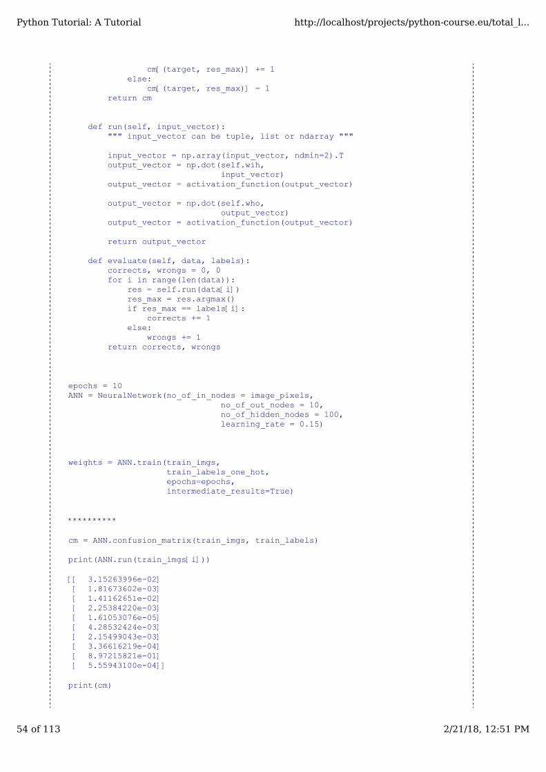
cm[(target, res_max)] += 1else:

cm[(target, res_max)] = 1return cm

def run(self, input_vector):

""" input_vector can be tuple, list or ndarray """

input_vector = np.array(input_vector, ndmin=2).Toutput_vector = np.dot(self.wih,





def evaluate(self, data, labels):

corrects, wrongs = 0, 0for i in range(len(data)):


corrects += 1else:


epochs = 10ANN = NeuralNetwork(no_of_in_nodes = image_pixels,


weights = ANN.train(train_imgs,train_labels_one_hot,epochs=epochs,intermediate_results=True)

**********

cm = ANN.confusion_matrix(train_imgs, train_labels) print(ANN.run(train_imgs[i]))

[[ 3.15263996e-02] [ 1.81673602e-03] [ 1.41162651e-02] [ 2.25384220e-03] [ 1.61053076e-05] [ 4.28532424e-03] [ 2.15499043e-03] [ 3.36616219e-04] [ 8.97215821e-01] [ 5.55943100e-04]]

print(cm)


54 of 113 2/21/18, 12:51 PM

{(5.0, 5): 5228, (0.0, 0): 5841, (4.0, 4): 5546, (1.0, 1): 6658, (9.0, 9): 5758, (2.0, 2): 5821, (3.0, 3): 5865, (6.0, 6): 5807, (7.0, 7): 6097, (8.0, 8): 5630, (7.0, 1): 30, (6.0, 0): 32, (9.0, 3): 29, (9.0, 0): 29, (5.0, 1): 4, (7.0, 8): 18, (1.0, 7): 8, (8.0, 1): 47, (3.0, 2): 56, (2.0, 0): 29, (5.0, 6): 38, (7.0, 0): 6, (4.0, 9): 191, (8.0, 2): 17, (2.0, 1): 14, (8.0, 5): 25, (5.0, 2): 6, (6.0, 4): 8, (0.0, 8): 35, (9.0, 2): 4, (3.0, 5): 51, (6.0, 8): 26, (4.0, 6): 35, (2.0, 7): 15, (6.0, 5): 29, (5.0, 8): 28, (2.0, 4): 12, (3.0, 7): 20, (5.0, 3): 67, (2.0, 6): 10, (4.0, 1): 8, (1.0, 4): 9, (8.0, 9): 30, (8.0, 7): 4, (3.0, 9): 38, (1.0, 8): 22, (3.0, 0): 26, (8.0, 6): 26, (8.0, 3): 36, (9.0, 5): 26, (9.0, 7): 21, (6.0, 1): 11, (7.0, 2): 32, (1.0, 9): 7, (7.0, 9): 57, (9.0, 1): 11, (9.0, 6): 4, (5.0, 9): 32, (8.0, 4): 21, (4.0, 2): 10, (2.0, 8): 25, (5.0, 7): 4, (1.0, 5): 6, (0.0, 2): 17, (1.0, 2): 22, (3.0, 8): 46, (3.0, 1): 8, (2.0, 5): 5, (6.0, 9): 2, (2.0, 9): 6, (0.0, 9): 5, (7.0, 4): 18, (9.0, 4): 38, (3.0, 6): 13, (3.0, 4): 8, (7.0, 6): 1, (8.0, 0): 15, (2.0, 3): 21, (0.0, 5): 1, (9.0, 8): 29, (4.0, 8): 35, (5.0, 0): 11, (1.0, 3): 8, (1.0, 6): 2, (0.0, 3): 4, (4.0, 0): 10, (6.0, 2): 2, (0.0, 6): 16, (7.0, 3): 5, (4.0, 7): 3, (4.0, 5): 3, (5.0, 4): 3, (6.0, 3): 1, (4.0, 3): 1, (0.0, 7): 1, (0.0, 4): 2, (7.0, 5): 1, (0.0, 1): 1}

for i in range(epochs): print("epoch: ", i)ANN.wih = weights[i][0]ANN.who = weights[i][1]


epoch: 0accruracy train: 0.9453166666666667accruracy: test 0.9448epoch: 1accruracy train: 0.95845accruracy: test 0.9519epoch: 2accruracy train: 0.96495accruracy: test 0.9581epoch: 3accruracy train: 0.9664166666666667accruracy: test 0.9577epoch: 4accruracy train: 0.9682accruracy: test 0.9575epoch: 5accruracy train: 0.9712833333333334accruracy: test 0.9579epoch: 6accruracy train: 0.97315accruracy: test 0.9573epoch: 7accruracy train: 0.9720833333333333accruracy: test 0.9587epoch: 8accruracy train: 0.9735666666666667accruracy: test 0.9591epoch: 9accruracy train: 0.97085accruracy: test 0.9569


55 of 113 2/21/18, 12:51 PM

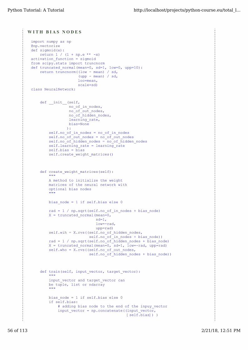
W I T H B I A S N O D E S






self.no_of_in_nodes = no_of_in_nodesself.no_of_out_nodes = no_of_out_nodes self.no_of_hidden_nodes = no_of_hidden_nodes self.learning_rate = learning_rateself.bias = biasself.create_weight_matrices()

def create_weight_matrices(self):"""

A method to initialize the weight matrices of the neural network with optional bias nodes """


rad = 1 / np.sqrt(self.no_of_in_nodes + bias_node)X = truncated_normal(mean=0,


self.wih = X.rvs((self.no_of_hidden_nodes,self.no_of_in_nodes + bias_node))

rad = 1 / np.sqrt(self.no_of_hidden_nodes + bias_node)X = truncated_normal(mean=0, sd=1, low=-rad, upp=rad)self.who = X.rvs((self.no_of_out_nodes,

self.no_of_hidden_nodes + bias_node))




# adding bias node to the end of the inpuy_vectorinput_vector = np.concatenate((input_vector,

[self.bias]) )


56 of 113 2/21/18, 12:51 PM


output_vector1 = np.dot(self.wih,input_vector)

output_hidden = activation_function(output_vector1)

if self.bias:output_hidden = np.concatenate((output_hidden,

[[self.bias]]) )

output_vector2 = np.dot(self.who,output_hidden)

output_network = activation_function(output_vector2)

output_errors = target_vector - output_network# update the weights:tmp = output_errors * output_network * (1.0 - output_network) tmp = self.learning_rate * np.dot(tmp, output_hidden.T)self.who += tmp# calculate hidden errors:hidden_errors = np.dot(self.who.T,

output_errors)# update the weights:tmp = hidden_errors * output_hidden * (1.0 - output_hidden)if self.bias:

x = np.dot(tmp, input_vector.T)[:-1,:] else:

x = np.dot(tmp, input_vector.T)self.wih += self.learning_rate * x

def run(self, input_vector):"""

input_vector can be tuple, list or ndarray """

if self.bias:# adding bias node to the end of the inpuy_vectorinput_vector = np.concatenate((input_vector, [1]) )

input_vector = np.array(input_vector, ndmin=2).Toutput_vector = np.dot(self.wih,


if self.bias:

output_vector = np.concatenate( (output_vector,[[1]]) )


output_vector)output_vector = activation_function(output_vector)return output_vector

def evaluate(self, data, labels):

corrects, wrongs = 0, 0for i in range(len(data)):


corrects += 1else:


57 of 113 2/21/18, 12:51 PM


ANN = NeuralNetwork(no_of_in_nodes=image_pixels,no_of_out_nodes=10,no_of_hidden_nodes=200,learning_rate=0.1,bias=None)


ANN.train(train_imgs[i], train_labels_one_hot[i])for i in range(20):

res = ANN.run(test_imgs[i])print(test_labels[i], np.argmax(res), np.max(res))

[ 7.] 7 0.991408237829[ 2.] 2 0.945947143112[ 1.] 1 0.989938832329[ 0.] 0 0.988126089612[ 4.] 4 0.962708218191[ 1.] 1 0.990239608255[ 4.] 4 0.98753488603[ 9.] 9 0.98375578053[ 5.] 9 0.438852313908[ 9.] 9 0.936706118303[ 0.] 0 0.958720609529[ 6.] 6 0.823852166595[ 9.] 9 0.986423262138[ 0.] 0 0.975261416069[ 1.] 1 0.992950534299[ 5.] 5 0.963848252707[ 9.] 9 0.99652758179[ 7.] 7 0.968342366695[ 3.] 3 0.808361646441[ 4.] 4 0.986540751733



VERSION WITH BIAS AND EPOCHS:





def __init__(self,


58 of 113 2/21/18, 12:51 PM

no_of_in_nodes,no_of_out_nodes,no_of_hidden_nodes,learning_rate,bias=None):

self.no_of_in_nodes = no_of_in_nodesself.no_of_out_nodes = no_of_out_nodes

self.no_of_hidden_nodes = no_of_hidden_nodes

self.learning_rate = learning_rateself.bias = biasself.create_weight_matrices()

def create_weight_matrices(self):"""

A method to initialize the weight matrices of the neural network with optional bias nodes"""


rad = 1 / np.sqrt(self.no_of_in_nodes + bias_node)X = truncated_normal(mean=0, sd=1, low=-rad, upp=rad)self.wih = X.rvs((self.no_of_hidden_nodes,

self.no_of_in_nodes + bias_node))rad = 1 / np.sqrt(self.no_of_hidden_nodes + bias_node)X = truncated_normal(mean=0,


self.who = X.rvs((self.no_of_out_nodes,self.no_of_hidden_nodes + bias_node))




# adding bias node to the end of the inpuy_vectorinput_vector = np.concatenate( (input_vector,

[self.bias]) )

output_vectors = []input_vector = np.array(input_vector, ndmin=2).Ttarget_vector = np.array(target_vector, ndmin=2).T



if self.bias:

output_hidden = np.concatenate((output_hidden,[[self.bias]]) )



output_errors = target_vector - output_network


59 of 113 2/21/18, 12:51 PM

# update the weights:tmp = output_errors * output_network * (1.0 - output_network)tmp = self.learning_rate * np.dot(tmp,

output_hidden.T)self.who += tmp

# calculate hidden errors:hidden_errors = np.dot(self.who.T,

output_errors)# update the weights:tmp = hidden_errors * output_hidden * (1.0 - output_hidden)if self.bias:

x = np.dot(tmp, input_vector.T)[:-1,:]else:


def train(self, data_array,

labels_one_hot_array,epochs=1,intermediate_results=False):


for i in range(len(data_array)):self.train_single(data_array[i],

labels_one_hot_array[i])if intermediate_results:

intermediate_weights.append((self.wih.copy(),self.who.copy()))

return intermediate_weights


if self.bias:


[self.bias]) )input_vector = np.array(input_vector, ndmin=2).Toutput_vector = np.dot(self.wih,


if self.bias:

output_vector = np.concatenate( (output_vector,[[self.bias]]) )






corrects += 1else:



60 of 113 2/21/18, 12:51 PM

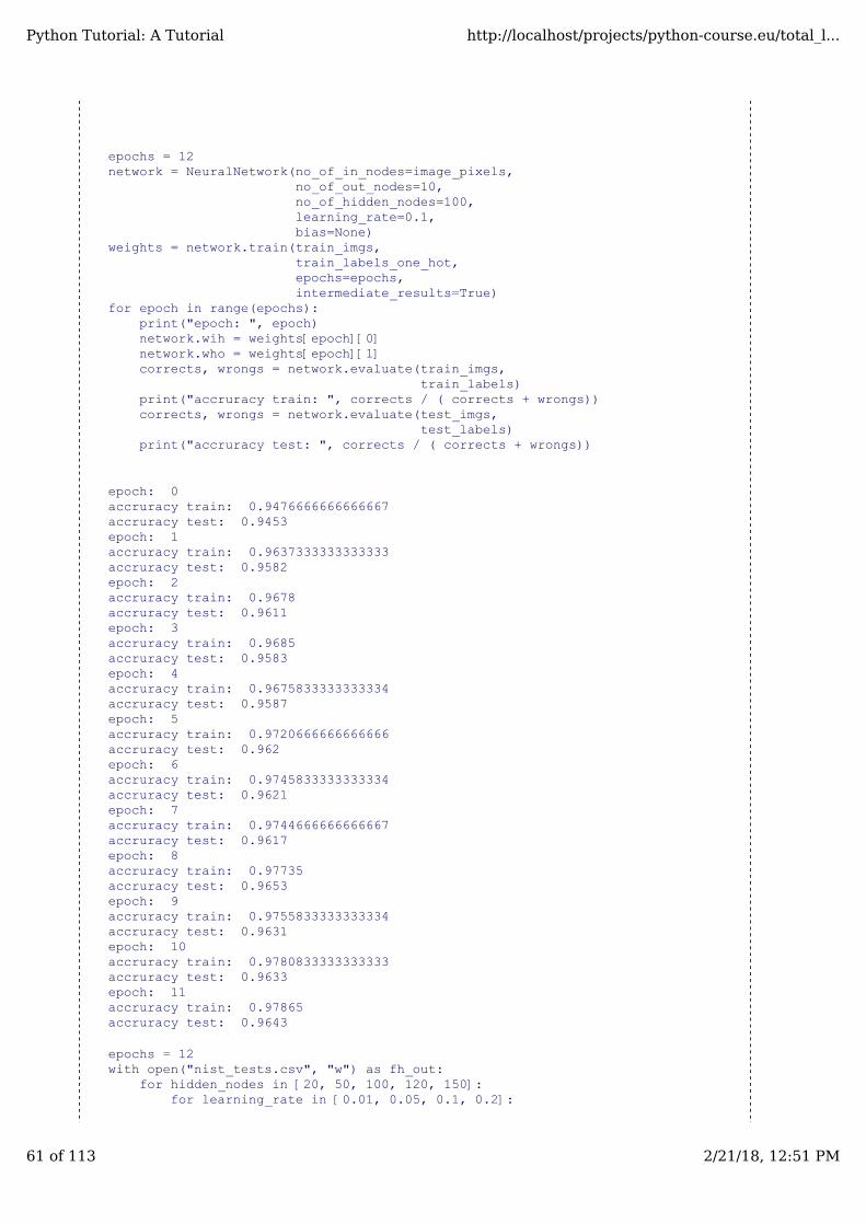
epochs = 12network = NeuralNetwork(no_of_in_nodes=image_pixels,

no_of_out_nodes=10,no_of_hidden_nodes=100,learning_rate=0.1,bias=None)

weights = network.train(train_imgs,train_labels_one_hot,epochs=epochs,intermediate_results=True)

for epoch in range(epochs): print("epoch: ", epoch)network.wih = weights[epoch][0]network.who = weights[epoch][1]corrects, wrongs = network.evaluate(train_imgs,

train_labels)print("accruracy train: ", corrects / ( corrects + wrongs))corrects, wrongs = network.evaluate(test_imgs,

test_labels)print("accruracy test: ", corrects / ( corrects + wrongs))

epoch: 0accruracy train: 0.9476666666666667accruracy test: 0.9453epoch: 1accruracy train: 0.9637333333333333accruracy test: 0.9582epoch: 2accruracy train: 0.9678accruracy test: 0.9611epoch: 3accruracy train: 0.9685accruracy test: 0.9583epoch: 4accruracy train: 0.9675833333333334accruracy test: 0.9587epoch: 5accruracy train: 0.9720666666666666accruracy test: 0.962epoch: 6accruracy train: 0.9745833333333334accruracy test: 0.9621epoch: 7accruracy train: 0.9744666666666667accruracy test: 0.9617epoch: 8accruracy train: 0.97735accruracy test: 0.9653epoch: 9accruracy train: 0.9755833333333334accruracy test: 0.9631epoch: 10accruracy train: 0.9780833333333333accruracy test: 0.9633epoch: 11accruracy train: 0.97865accruracy test: 0.9643

epochs = 12with open("nist_tests.csv", "w") as fh_out:

for hidden_nodes in [20, 50, 100, 120, 150]:for learning_rate in [0.01, 0.05, 0.1, 0.2]:


61 of 113 2/21/18, 12:51 PM

for bias in [None, 0.5]:network = NeuralNetwork(no_of_in_nodes=image_pixels,

no_of_out_nodes=10,no_of_hidden_nodes=hidden_nodes,learning_rate=learning_rate,bias=bias)

weights = network.train(train_imgs,train_labels_one_hot,epochs=epochs,intermediate_results=True)

for epoch in range(epochs): print("*", end="")network.wih = weights[epoch][0]network.who = weights[epoch][1]train_corrects, train_wrongs =

network.evaluate(train_imgs,

train_labels)

test_corrects, test_wrongs = network.evaluate(test_imgs,test_labels)

outstr = str(hidden_nodes) + " " + str(learning_rate) + " " + str(bias)

outstr += " " + str(epoch) + " "outstr += str(train_corrects / (train_corrects +

train_wrongs)) + " "outstr += str(train_wrongs / (train_corrects +

train_wrongs)) + " "outstr += str(test_corrects / (test_corrects +

test_wrongs)) + " "outstr += str(test_wrongs / (test_corrects + test_wrongs))

fh_out.write(outstr + "\n" )fh_out.flush()

The file nist_tests_20_50_100_120_150.csv contains the results from a run of the previous program.


62 of 113 2/21/18, 12:51 PM

N E T W O R K S W I T H M U LT I P L E H I D D E N L AY E R S

We will write a new neural network class, in which we can define an arbitrary number of hidden layers. The code is alsoimproved, because the weight matrices are now build inside of a loop instead redundant code:




def __init__(self,network_structure, # ie. [input_nodes, hidden1_nodes, ... ,

hidden_n_nodes, output_nodes]learning_rate,bias=None):

self.structure = network_structureself.learning_rate = learning_rateself.bias = biasself.create_weight_matrices()


bias_node = 1 if self.bias else 0self.weights_matrices = []

layer_index = 1no_of_layers = len(self.structure)while layer_index < no_of_layers:

nodes_in = self.structure[layer_index-1]nodes_out = self.structure[layer_index]n = (nodes_in + bias_node) * nodes_outrad = 1 / np.sqrt(nodes_in)X = truncated_normal(mean=2,


wm = X.rvs(n).reshape((nodes_out, nodes_in + bias_node))self.weights_matrices.append(wm)layer_index += 1



no_of_layers = len(self.structure)input_vector = np.array(input_vector, ndmin=2).Tlayer_index = 0# The output/input vectors of the various layers:res_vectors = [input_vector]while layer_index < no_of_layers - 1:

in_vector = res_vectors[-1]if self.bias:

# adding bias node to the end of the 'input'_vectorin_vector = np.concatenate( (in_vector,

[[self.bias]]) )res_vectors[-1] = in_vector


63 of 113 2/21/18, 12:51 PM

x = np.dot(self.weights_matrices[layer_index],in_vector)

out_vector = activation_function(x)# the output of one layer is the input of the next one:res_vectors.append(out_vector)layer_index += 1

layer_index = no_of_layers - 1target_vector = np.array(target_vector, ndmin=2).T# The input vectors to the various layersoutput_errors = target_vector - out_vector while layer_index > 0:

out_vector = res_vectors[layer_index]in_vector = res_vectors[layer_index-1]if self.bias and not layer_index==(no_of_layers-1):

out_vector = out_vector[:-1,:].copy()tmp = output_errors * out_vector * (1.0 - out_vector) tmp = np.dot(tmp, in_vector.T)

#if self.bias:# tmp = tmp[:-1,:]

self.weights_matrices[layer_index-1] += self.learning_rate * tmp

output_errors = np.dot(self.weights_matrices[layer_index-1].T,

output_errors)if self.bias:

output_errors = output_errors[:-1,:]layer_index -= 1

def run(self, input_vector):# input_vector can be tuple, list or ndarrayno_of_layers = len(self.structure)if self.bias:


[self.bias]) )in_vector = np.array(input_vector, ndmin=2).Tlayer_index = 1# The input vectors to the various layerswhile layer_index < no_of_layers:

x = np.dot(self.weights_matrices[layer_index-1],in_vector)

out_vector = activation_function(x)

# input vector for next layerin_vector = out_vectorif self.bias:

in_vector = np.concatenate( (in_vector,[[self.bias]]) )

layer_index += 1

return out_vector



corrects += 1


64 of 113 2/21/18, 12:51 PM

else:wrongs += 1

return corrects, wrongs

ANN = NeuralNetwork(network_structure=[image_pixels, 50, 50, 10],learning_rate=0.1,bias=None)


ANN.train(train_imgs[i], train_labels_one_hot[i])




65 of 113 2/21/18, 12:51 PM

N E T W O R K S W I T H M U LT I P L E H I D D E N L AY E R S A N D E P O C H S




def __init__(self,network_structure, # ie. [input_nodes, hidden1_nodes, ... ,

hidden_n_nodes, output_nodes]learning_rate,bias=None):

self.structure = network_structureself.learning_rate = learning_rateself.bias = biasself.create_weight_matrices()

def create_weight_matrices(self):X = truncated_normal(mean=2, sd=1, low=-0.5, upp=0.5)

bias_node = 1 if self.bias else 0self.weights_matrices = [] layer_index = 1no_of_layers = len(self.structure)while layer_index < no_of_layers:

nodes_in = self.structure[layer_index-1]nodes_out = self.structure[layer_index]n = (nodes_in + bias_node) * nodes_outrad = 1 / np.sqrt(nodes_in)X = truncated_normal(mean=2, sd=1, low=-rad, upp=rad)wm = X.rvs(n).reshape((nodes_out, nodes_in + bias_node))self.weights_matrices.append(wm)layer_index += 1

def train_single(self, input_vector, target_vector):# input_vector and target_vector can be tuple, list or ndarray

no_of_layers = len(self.structure) input_vector = np.array(input_vector, ndmin=2).Tlayer_index = 0# The output/input vectors of the various layers:res_vectors = [input_vector] while layer_index < no_of_layers - 1:

in_vector = res_vectors[-1]if self.bias:

# adding bias node to the end of the 'input'_vectorin_vector = np.concatenate( (in_vector,

[[self.bias]]) )res_vectors[-1] = in_vector

x = np.dot(self.weights_matrices[layer_index], in_vector)out_vector = activation_function(x)res_vectors.append(out_vector) layer_index += 1

layer_index = no_of_layers - 1target_vector = np.array(target_vector, ndmin=2).T# The input vectors to the various layers


66 of 113 2/21/18, 12:51 PM

output_errors = target_vector - out_vector while layer_index > 0:

out_vector = res_vectors[layer_index]in_vector = res_vectors[layer_index-1]if self.bias and not layer_index==(no_of_layers-1):

out_vector = out_vector[:-1,:].copy()tmp = output_errors * out_vector * (1.0 - out_vector) tmp = np.dot(tmp, in_vector.T)

#if self.bias:# tmp = tmp[:-1,:]

self.weights_matrices[layer_index-1] += self.learning_rate * tmp

output_errors = np.dot(self.weights_matrices[layer_index-1].T,

output_errors)if self.bias:

output_errors = output_errors[:-1,:]layer_index -= 1

def train(self, data_array,labels_one_hot_array,epochs=1,intermediate_results=False):


for i in range(len(data_array)):self.train_single(data_array[i], labels_one_hot_array[i])

if intermediate_results:intermediate_weights.append((self.wih.copy(),

self.who.copy()))return intermediate_weights

def run(self, input_vector):# input_vector can be tuple, list or ndarrayno_of_layers = len(self.structure)if self.bias:

# adding bias node to the end of the inpuy_vectorinput_vector = np.concatenate( (input_vector, [self.bias]) )

in_vector = np.array(input_vector, ndmin=2).Tlayer_index = 1# The input vectors to the various layerswhile layer_index < no_of_layers:

x = np.dot(self.weights_matrices[layer_index-1],in_vector)

out_vector = activation_function(x)

# input vector for next layerin_vector = out_vectorif self.bias:

in_vector = np.concatenate( (in_vector,[[self.bias]]) )

layer_index += 1

return out_vector


res = self.run(data[i])res_max = res.argmax()


67 of 113 2/21/18, 12:51 PM

if res_max == labels[i]:corrects += 1

else:wrongs += 1

return corrects, wrongs

epochs = 3ANN = NeuralNetwork(network_structure=[image_pixels, 80, 80, 10],

learning_rate=0.01,bias=None)

ANN.train(train_imgs, train_labels_one_hot, epochs=epochs)


[]



FOOTNOTES

1 Wan, Li; Matthew Zeiler; Sixin Zhang; Yann LeCun; Rob Fergus (2013). Regularization of Neural Network usingDropConnect. International Conference on Machine Learning(ICML).


68 of 113 2/21/18, 12:51 PM

D R O P O U T N E U R A L N E T W O R K S

INTRODUCTION

The term "dropout" is used for a technique which dropsout some nodes of the network. Dropping out can beseen as temporarily deactivating or ignoring neurons ofthe network. This technique is applied in the trainingphase to reduce overfitting effects. Overfitting is anerror which occurs when a network is too closely fit toa limited set of input samples.

The basic idea behind dropout neural networks is todropout nodes so that the network can concentrate onother features. Think about it like this. You watch lotsof films from your favourite actor. At some point youlisten to the radio and here somebody in an interview.You don't recognize your favourite actor, because youhave seen only movies and your are a visual type. Now,imagine that you can only listen to the audio tracks ofthe films. In this case you will have to learn todifferentiate the voices of the actresses and actors. Soby dropping out the visual part you are forced tp focuson the sound features!

This technique has been first proposed in a paper "Dropout: A Simple Way to Prevent Neural Networks from Overfitting"by Nitish Srivastava, Geoffrey Hinton, Alex Krizhevsky, Ilya Sutskever and Ruslan Salakhutdinov in 2014

We will implement in our tutorial on machine learning in Python a Python class which is capable of dropout.

MODIFYING THE WEIGHT ARRAYS

If we deactivate a node, we have to modify the weight arrays accordingly. To demonstrate how this can be accomplished,we will use a network with three input nodes, four hidden and two output nodes:

At first, we will have a look at the weight array between the input and the hidden layer. We called this array 'wih' (weightsbetween input and hidden layer).

Let's deactivate (drop out) the node . We can see in the following diagram what's happening:i2


69 of 113 2/21/18, 12:51 PM

This means that we have to take out every second product of the summation, which means that we have to delete thewhole second column of the matrix. The second element from the input vector has to be deleted as well.

Now we will examine what happens if we take out a hidden node. We take out the first hidden node, i.e. .

In this case, we can remove the complete first line of our weight matrix:

Taking out a hidden node affects the next weight matrix as well. Let's have a look at what is happening in the networkgraph:

h1


70 of 113 2/21/18, 12:51 PM

It is easy to see that the first column of the who weight matrix has to be removed again:

So far we have arbitrarily chosen one node to deactivate. The dropout approach means that we randomly choose a certainnumber of nodes from the input and the hidden layers, which remain active and turn off the other nodes of these layers.After this we can train a part of our learn set with this network. The next step consists in activating all the nodes again andrandomly chose other nodes. It is also possible to train the whole training set with the randomly created dropout networks.

We present three possible randomly chosen dropout networks in the following three diagrams:

Now it is time to think about a possible Python implementation.

We will start with the weight matrix between input and hidden layer. We will randomly create a weight matrix for 10 inputnodes and 5 hidden nodes. We fill our matrix with random numbers between -10 and 10, which are not proper weightvalues, but this way we can see better what is going on:

import numpy as npimport randominput_nodes = 10hidden_nodes = 5output_nodes = 7wih = np.random.randint(-10, 10, (hidden_nodes, input_nodes))wih

The above Python code returned the following result:

array([[ -6, -8, -3, -7, 2, -9, -3, -5, -6, 4], [ 5, 3, 7, -4, 4, 8, -2, -4, 7, 7], [ 9, -7, 4, 0, 4, 0, -3, -6, -2, 7], [ -8, -9, -4, -5, -9, 8, -8, -8, -2, -3], [ 3, -10, 0, -3, 4, 0, 0, 2, -7, -9]])

We will choose now the active nodes for the input layer. We calculate random indices for the active nodes:

active_input_percentage = 0.7active_input_nodes = int(input_nodes * active_input_percentage)active_input_indices = sorted(random.sample(range(0, input_nodes),

active_input_nodes))active_input_indices

The above Python code returned the following:

[0, 1, 2, 5, 7, 8, 9]

We learned above that we have to remove the column , if the node is removed. We can easily accomplish this for alldeactived nodes by using the slicing operator with the active nodes:

wih_old = wih.copy()

j ij


71 of 113 2/21/18, 12:51 PM

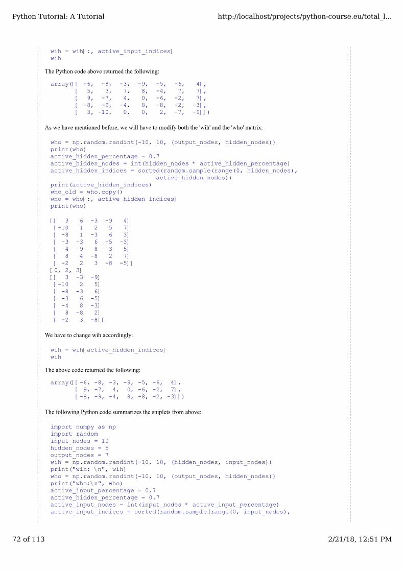
wih = wih[:, active_input_indices]wih


array([[ -6, -8, -3, -9, -5, -6, 4], [ 5, 3, 7, 8, -4, 7, 7], [ 9, -7, 4, 0, -6, -2, 7], [ -8, -9, -4, 8, -8, -2, -3], [ 3, -10, 0, 0, 2, -7, -9]])

As we have mentioned before, we will have to modify both the 'wih' and the 'who' matrix:

who = np.random.randint(-10, 10, (output_nodes, hidden_nodes))print(who)active_hidden_percentage = 0.7active_hidden_nodes = int(hidden_nodes * active_hidden_percentage)active_hidden_indices = sorted(random.sample(range(0, hidden_nodes),

active_hidden_nodes))print(active_hidden_indices)who_old = who.copy()who = who[:, active_hidden_indices]print(who)

[[ 3 6 -3 -9 4] [-10 1 2 5 7] [ -8 1 -3 6 3] [ -3 -3 6 -5 -3] [ -4 -9 8 -3 5] [ 8 4 -8 2 7] [ -2 2 3 -8 -5]][0, 2, 3][[ 3 -3 -9] [-10 2 5] [ -8 -3 6] [ -3 6 -5] [ -4 8 -3] [ 8 -8 2] [ -2 3 -8]]

We have to change wih accordingly:

wih = wih[active_hidden_indices]wih


array([[-6, -8, -3, -9, -5, -6, 4], [ 9, -7, 4, 0, -6, -2, 7], [-8, -9, -4, 8, -8, -2, -3]])

The following Python code summarizes the sniplets from above:

import numpy as npimport randominput_nodes = 10hidden_nodes = 5output_nodes = 7wih = np.random.randint(-10, 10, (hidden_nodes, input_nodes))print("wih: \n", wih)who = np.random.randint(-10, 10, (output_nodes, hidden_nodes))print("who:\n", who)active_input_percentage = 0.7active_hidden_percentage = 0.7active_input_nodes = int(input_nodes * active_input_percentage)active_input_indices = sorted(random.sample(range(0, input_nodes),


72 of 113 2/21/18, 12:51 PM

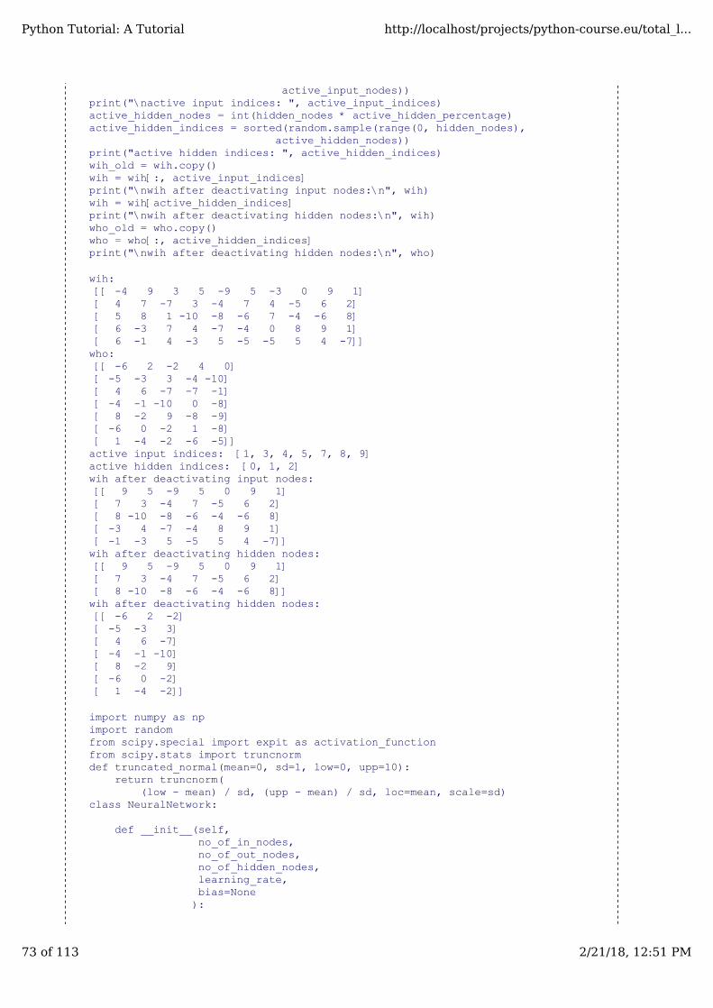
active_input_nodes))print("\nactive input indices: ", active_input_indices)active_hidden_nodes = int(hidden_nodes * active_hidden_percentage)active_hidden_indices = sorted(random.sample(range(0, hidden_nodes),

active_hidden_nodes))print("active hidden indices: ", active_hidden_indices)wih_old = wih.copy()wih = wih[:, active_input_indices]print("\nwih after deactivating input nodes:\n", wih)wih = wih[active_hidden_indices]print("\nwih after deactivating hidden nodes:\n", wih)who_old = who.copy()who = who[:, active_hidden_indices]print("\nwih after deactivating hidden nodes:\n", who)

wih: [[ -4 9 3 5 -9 5 -3 0 9 1] [ 4 7 -7 3 -4 7 4 -5 6 2] [ 5 8 1 -10 -8 -6 7 -4 -6 8] [ 6 -3 7 4 -7 -4 0 8 9 1] [ 6 -1 4 -3 5 -5 -5 5 4 -7]]who: [[ -6 2 -2 4 0] [ -5 -3 3 -4 -10] [ 4 6 -7 -7 -1] [ -4 -1 -10 0 -8] [ 8 -2 9 -8 -9] [ -6 0 -2 1 -8] [ 1 -4 -2 -6 -5]]active input indices: [1, 3, 4, 5, 7, 8, 9]active hidden indices: [0, 1, 2]wih after deactivating input nodes: [[ 9 5 -9 5 0 9 1] [ 7 3 -4 7 -5 6 2] [ 8 -10 -8 -6 -4 -6 8] [ -3 4 -7 -4 8 9 1] [ -1 -3 5 -5 5 4 -7]]wih after deactivating hidden nodes: [[ 9 5 -9 5 0 9 1] [ 7 3 -4 7 -5 6 2] [ 8 -10 -8 -6 -4 -6 8]]wih after deactivating hidden nodes: [[ -6 2 -2] [ -5 -3 3] [ 4 6 -7] [ -4 -1 -10] [ 8 -2 9] [ -6 0 -2] [ 1 -4 -2]]

import numpy as npimport randomfrom scipy.special import expit as activation_functionfrom scipy.stats import truncnormdef truncated_normal(mean=0, sd=1, low=0, upp=10):





73 of 113 2/21/18, 12:51 PM

self.no_of_in_nodes = no_of_in_nodesself.no_of_out_nodes = no_of_out_nodes self.no_of_hidden_nodes = no_of_hidden_nodes self.learning_rate = learning_rateself.bias = biasself.create_weight_matrices()


X = truncated_normal(mean=2, sd=1, low=-0.5, upp=0.5)

bias_node = 1 if self.bias else 0n = (self.no_of_in_nodes + bias_node) * self.no_of_hidden_nodesX = truncated_normal(mean=2, sd=1, low=-0.5, upp=0.5)self.wih = X.rvs(n).reshape((self.no_of_hidden_nodes,

self.no_of_in_nodes +bias_node))

n = (self.no_of_hidden_nodes + bias_node) * self.no_of_out_nodesX = truncated_normal(mean=2, sd=1, low=-0.5, upp=0.5)self.who = X.rvs(n).reshape((self.no_of_out_nodes,

(self.no_of_hidden_nodes +bias_node)))

def dropout_weight_matrices(self,active_input_percentage=0.70,active_hidden_percentage=0.70):

# restore wih array, if it had been used for dropoutself.wih_orig = self.wih.copy()self.no_of_in_nodes_orig = self.no_of_in_nodesself.no_of_hidden_nodes_orig = self.no_of_hidden_nodesself.who_orig = self.who.copy()

active_input_nodes = int(self.no_of_in_nodes *

active_input_percentage)active_input_indices = sorted(random.sample(range(0,

self.no_of_in_nodes),active_input_nodes))

active_hidden_nodes = int(self.no_of_hidden_nodes *active_hidden_percentage)

active_hidden_indices = sorted(random.sample(range(0,self.no_of_hidden_nodes),

active_hidden_nodes))

self.wih = self.wih[:, active_input_indices][active_hidden_indices]self.who = self.who[:, active_hidden_indices]

self.no_of_hidden_nodes = active_hidden_nodesself.no_of_in_nodes = active_input_nodesreturn active_input_indices, active_hidden_indices

def weight_matrices_reset(self,

active_input_indices,active_hidden_indices):

"""

self.wih and self.who contain the newly adapted values from the active nodes. We have to reconstruct the original weight matrices by assigning the new values from the active nodes """

temp = self.wih_orig.copy()[:,active_input_indices]temp[active_hidden_indices] = self.wihself.wih_orig[:, active_input_indices] = tempself.wih = self.wih_orig.copy()self.who_orig[:, active_hidden_indices] = self.whoself.who = self.who_orig.copy()


74 of 113 2/21/18, 12:51 PM

self.no_of_in_nodes = self.no_of_in_nodes_origself.no_of_hidden_nodes = self.no_of_hidden_nodes_orig



if self.bias:# adding bias node to the end of the input_vectorinput_vector = np.concatenate( (input_vector, [self.bias]) )

input_vector = np.array(input_vector, ndmin=2).Ttarget_vector = np.array(target_vector, ndmin=2).Toutput_vector1 = np.dot(self.wih, input_vector)output_vector_hidden = activation_function(output_vector1)

if self.bias:

output_vector_hidden = np.concatenate( (output_vector_hidden,[[self.bias]]) )

output_vector2 = np.dot(self.who, output_vector_hidden)output_vector_network = activation_function(output_vector2)


output_vector_network) tmp = self.learning_rate * np.dot(tmp, output_vector_hidden.T)self.who += tmp# calculate hidden errors:hidden_errors = np.dot(self.who.T, output_errors)# update the weights:tmp = hidden_errors * output_vector_hidden * (1.0 -

output_vector_hidden)if self.bias:

x = np.dot(tmp, input_vector.T)[:-1,:]else:


def train(self, data_array,labels_one_hot_array,epochs=1,active_input_percentage=0.70,active_hidden_percentage=0.70,no_of_dropout_tests = 10):

partition_length = int(len(data_array) / no_of_dropout_tests)

for epoch in range(epochs):print("epoch: ", epoch)for start in range(0, len(data_array), partition_length):

active_in_indices, active_hidden_indices = \

self.dropout_weight_matrices(active_input_percentage,

active_hidden_percentage)for i in range(start, start + partition_length):

self.train_single(data_array[i][active_in_indices],labels_one_hot_array[i])

self.weight_matrices_reset(active_in_indices,

active_hidden_indices)


75 of 113 2/21/18, 12:51 PM

def confusion_matrix(self, data_array, labels):

cm = {}for i in range(len(data_array)):

res = self.run(data_array[i])res_max = res.argmax()target = labels[i][0]if (target, res_max) in cm:

cm[(target, res_max)] += 1else:

cm[(target, res_max)] = 1return cm


if self.bias:

# adding bias node to the end of the input_vectorinput_vector = np.concatenate( (input_vector, [self.bias]) )

input_vector = np.array(input_vector, ndmin=2).Toutput_vector = np.dot(self.wih, input_vector)output_vector = activation_function(output_vector)

if self.bias:

output_vector = np.concatenate( (output_vector, [[self.bias]]) )

output_vector = np.dot(self.who, output_vector)output_vector = activation_function(output_vector)




corrects += 1else:


import picklewith open("data/mnist/pickled_mnist.pkl", "br") as fh:

data = pickle.load(fh)train_imgs = data[0]test_imgs = data[1]train_labels = data[2]test_labels = data[3]train_labels_one_hot = data[4]test_labels_one_hot = data[5]image_size = 28 # width and lengthno_of_different_labels = 10 # i.e. 0, 1, 2, 3, ..., 9image_pixels = image_size * image_size

In [ ]:

parts = 10partition_length = int(len(train_imgs) / parts)print(partition_length)start = 0for start in range(0, len(train_imgs), partition_length):

print(start, start + partition_length)

6000


76 of 113 2/21/18, 12:51 PM

0 60006000 1200012000 1800018000 2400024000 3000030000 3600036000 4200042000 4800048000 5400054000 60000

In [ ]:

epochs = 3simple_network = NeuralNetwork(no_of_in_nodes = image_pixels,


simple_network.train(train_imgs,train_labels_one_hot,active_input_percentage=1,active_hidden_percentage=1,no_of_dropout_tests = 100,epochs=epochs)

epoch: 0

In [ ]:

corrects, wrongs = simple_network.evaluate(train_imgs, train_labels)print("accruracy train: ", corrects / ( corrects + wrongs))corrects, wrongs = simple_network.evaluate(test_imgs, test_labels)print("accruracy: test", corrects / ( corrects + wrongs))


77 of 113 2/21/18, 12:51 PM

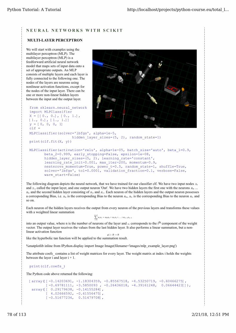
N E U R A L N E T W O R K S W I T H S C I K I T

MULTI-LAYER PERCEPTRON

We will start with examples using themultilayer perceptron (MLP). Themultilayer perceptron (MLP) is afeedforward artificial neural networkmodel that maps sets of input data onto aset of appropriate outputs. An MLPconsists of multiple layers and each layer isfully connected to the following one. Thenodes of the layers are neurons usingnonlinear activation functions, except forthe nodes of the input layer. There can beone or more non-linear hidden layersbetween the input and the output layer.

from sklearn.neural_networkimport MLPClassifierX = [[0., 0.], [0., 1.],[1., 0.], [1., 1.]]y = [0, 0, 0, 1]clf =MLPClassifier(solver='lbfgs', alpha=1e-5,

hidden_layer_sizes=(5, 2), random_state=1)print(clf.fit(X, y))

MLPClassifier(activation='relu', alpha=1e-05, batch_size='auto', beta_1=0.9, beta_2=0.999, early_stopping=False, epsilon=1e-08, hidden_layer_sizes=(5, 2), learning_rate='constant', learning_rate_init=0.001, max_iter=200, momentum=0.9, nesterovs_momentum=True, power_t=0.5, random_state=1, shuffle=True, solver='lbfgs', tol=0.0001, validation_fraction=0.1, verbose=False, warm_start=False)

The following diagram depicts the neural network, that we have trained for our classifier clf. We have two input nodes and , called the input layer, and one output neuron 'Out'. We have two hidden layers the first one with the neurons ...

and the second hidden layer consisting of and . Each neuron of the hidden layers and the output neuron possessesa corresponding Bias, i.e. is the corresponding Bias to the neuron , is the corresponding Bias to the neuron andso on.

Each neuron of the hidden layers receives the output from every neuron of the previous layers and transforms these valueswith a weighted linear summation

into an output value, where n is the number of neurons of the layer and corresponds to the ith component of the weightvector. The output layer receives the values from the last hidden layer. It also performs a linear summation, but a non-linear activation function

like the hyperbolic tan function will be applied to the summation result.

%matplotlib inline from IPython.display import Image Image(filename='images/mlp_example_layer.png')

The attribute coefs_ contains a list of weight matrices for every layer. The weight matrix at index i holds the weightsbetween the layer i and layer i + 1.

print(clf.coefs_)


[array([[-0.14203691, -1.18304359, -0.85567518, -4.53250719, -0.60466275], [-0.69781111, -3.5850093 , -0.26436018, -4.39161248, 0.06644423]]), array([[ 0.29179638, -0.14155284], [ 4.02666592, -0.61556475], [-0.51677234, 0.51479708],

X0

X1 H00

H04 H10 H11

B00 H00 B01 H01

= + +. . . +∑i=0

n−1

wixi w0x0 w1x1 wn−1xn−1

wi

g(⋅) : R→ R


78 of 113 2/21/18, 12:51 PM

[ 7.37215202, -0.31936965], [ 0.32920668, 0.64428109]]), array([[-4.96774269], [-0.86330397]])]

The summation formula of the neuronH00 is defined by:

which can be written as

because .

We can get the values for and fromclf.coefs_ like this:

clf.coefs_[0][0][0] and clf.coefs_[0][1][0]

print("w0 = ", clf.coefs_[0][0][0])print("w1 = ", clf.coefs_[0][1][0])

w0 = -0.142036912678w1 = -0.697811114978

The weight vector of can be accessed with

clf.coefs_[0][:,0]


array([-0.14203691, -0.69781111])

We can generalize the above to access a neuron in the following way:

for i in range(len(clf.coefs_)):number_neurons_in_layer = clf.coefs_[i].shape[1]for j in range(number_neurons_in_layer):

weights = clf.coefs_[i][:,j]print(i, j, weights, end=", ")print()

print()

0 0 [-0.14203691 -0.69781111], 0 1 [-1.18304359 -3.5850093 ], 0 2 [-0.85567518 -0.26436018], 0 3 [-4.53250719 -4.39161248], 0 4 [-0.60466275 0.06644423], 1 0 [ 0.29179638 4.02666592 -0.51677234 7.37215202 0.32920668], 1 1 [-0.14155284 -0.61556475 0.51479708 -0.31936965 0.64428109], 2 0 [-4.96774269 -0.86330397],

intercepts_ is a list of bias vectors, where the vector at index i represents the bias values added to layer i+1.

print(clf.intercepts_)

The above Python code returned the following output:

[array([-0.14962269, -0.59232707, -0.5472481 , 7.02667699, -0.87510813]), array([-3.61417672, -0.76834882]), array([ 8.48188176])]

= + + ∗∑i=0

n−1

wixi w0x0 w1x1 wB11 B11

= + +∑i=0

n−1

wixi w0x0 w1x1 wB11

= 1B11

w0 w1

=w0 =w1

H00

Hij


79 of 113 2/21/18, 12:51 PM

The main reason, why we train a classifier is to predict results for new samples. We can do this with the predict method.The method returns a predicted class for a sample, in our case a "0" or a "1" :

result = clf.predict([[0, 0], [0, 1],[1, 0], [0, 1],[1, 1], [2., 2.],[1.3, 1.3], [2, 4.8]])

Instead of just looking at the class results, we can also use the predict_proba method to get the probability estimates.

prob_results = clf.predict_proba([[0, 0], [0, 1],[1, 0], [0, 1],[1, 1], [2., 2.],[1.3, 1.3], [2, 4.8]])

print(prob_results)

[[ 1.00000000e+000 5.25723951e-101] [ 1.00000000e+000 3.71534882e-031] [ 1.00000000e+000 6.47069178e-029] [ 1.00000000e+000 3.71534882e-031] [ 2.07145538e-004 9.99792854e-001] [ 2.07145538e-004 9.99792854e-001] [ 2.07145538e-004 9.99792854e-001] [ 2.07145538e-004 9.99792854e-001]]

prob_results[i][0] gives us the probability for the class0, i.e. a "0" and results[i][1] the probabilty for a "1". i correspondsto the ith sample.

ANOTHER EXAMPLE

We will populate to clusters (class0 and class1) in a two dimensional space.

import numpy as npfrom matplotlib import pyplot as pltnpoints = 50X, Y = [], []# class 0X.append(np.random.uniform(low=-2.5, high=2.3, size=(npoints,)) )Y.append(np.random.uniform(low=-1.7, high=2.8, size=(npoints,)))# class 1X.append(np.random.uniform(low=-7.2, high=-4.4, size=(npoints,)) )Y.append(np.random.uniform(low=3, high=6.5, size=(npoints,)))learnset = []learnlabels = []for i in range(2):

# adding points of class i to learnsetpoints = zip(X[i], Y[i])for p in points:

learnset.append(p)learnlabels.append(i)

npoints_test = 3 * npointsTestX = np.random.uniform(low=-7.2, high=5, size=(npoints_test,))TestY = np.random.uniform(low=-4, high=9, size=(npoints_test,))testset = []points = zip(TestX, TestY)for p in points:

testset.append(p)colours = ["b", "r"]for i in range(2):

plt.scatter(X[i], Y[i], c=colours[i])plt.scatter(TestX, TestY, c="g")plt.show()


80 of 113 2/21/18, 12:51 PM

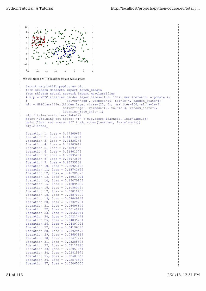
We will train a MLPClassifier for out two classes:

import matplotlib.pyplot as pltfrom sklearn.datasets import fetch_mldatafrom sklearn.neural_network import MLPClassifier# mlp = MLPClassifier(hidden_layer_sizes=(100, 100), max_iter=400, alpha=1e-4,# solver='sgd', verbose=10, tol=1e-4, random_state=1)mlp = MLPClassifier(hidden_layer_sizes=(20, 3), max_iter=150, alpha=1e-4,

solver='sgd', verbose=10, tol=1e-4, random_state=1,learning_rate_init=.1)

mlp.fit(learnset, learnlabels)print("Training set score: %f" % mlp.score(learnset, learnlabels))print("Test set score: %f" % mlp.score(learnset, learnlabels))mlp.classes_

Iteration 1, loss = 0.47209614Iteration 2, loss = 0.44614294Iteration 3, loss = 0.41336245Iteration 4, loss = 0.37903617Iteration 5, loss = 0.34893492Iteration 6, loss = 0.31801372Iteration 7, loss = 0.28795204Iteration 8, loss = 0.25973898Iteration 9, loss = 0.23339132Iteration 10, loss = 0.20923182Iteration 11, loss = 0.18742655Iteration 12, loss = 0.16785779Iteration 13, loss = 0.15037921Iteration 14, loss = 0.13479158Iteration 15, loss = 0.12095939Iteration 16, loss = 0.10880727Iteration 17, loss = 0.09810485Iteration 18, loss = 0.08870370Iteration 19, loss = 0.08049147Iteration 20, loss = 0.07329201Iteration 21, loss = 0.06696649Iteration 22, loss = 0.06140222Iteration 23, loss = 0.05650041Iteration 24, loss = 0.05217473Iteration 25, loss = 0.04835234Iteration 26, loss = 0.04497095Iteration 27, loss = 0.04196786Iteration 28, loss = 0.03929475Iteration 29, loss = 0.03690869Iteration 30, loss = 0.03477277Iteration 31, loss = 0.03285525Iteration 32, loss = 0.03112890Iteration 33, loss = 0.02957041Iteration 34, loss = 0.02815974Iteration 35, loss = 0.02687962Iteration 36, loss = 0.02571506Iteration 37, loss = 0.02465300


81 of 113 2/21/18, 12:51 PM

Iteration 38, loss = 0.02368203Iteration 39, loss = 0.02279213Iteration 40, loss = 0.02197453Iteration 41, loss = 0.02122149Iteration 42, loss = 0.02052625Iteration 43, loss = 0.01988283Iteration 44, loss = 0.01928600Iteration 45, loss = 0.01873112Iteration 46, loss = 0.01821413Iteration 47, loss = 0.01773141Iteration 48, loss = 0.01727976Iteration 49, loss = 0.01685633Iteration 50, loss = 0.01645859Iteration 51, loss = 0.01608425Iteration 52, loss = 0.01573129Iteration 53, loss = 0.01539788Iteration 54, loss = 0.01508238Iteration 55, loss = 0.01478333Iteration 56, loss = 0.01449938Iteration 57, loss = 0.01422935Iteration 58, loss = 0.01397216Iteration 59, loss = 0.01372683Iteration 60, loss = 0.01349248Iteration 61, loss = 0.01326831Iteration 62, loss = 0.01305360Iteration 63, loss = 0.01284768Iteration 64, loss = 0.01264995Iteration 65, loss = 0.01245986Iteration 66, loss = 0.01227692Iteration 67, loss = 0.01210067Iteration 68, loss = 0.01193067Iteration 69, loss = 0.01176657Iteration 70, loss = 0.01160798Iteration 71, loss = 0.01145461Iteration 72, loss = 0.01130613Iteration 73, loss = 0.01116229Iteration 74, loss = 0.01102282Iteration 75, loss = 0.01088750Iteration 76, loss = 0.01075610Iteration 77, loss = 0.01062842Iteration 78, loss = 0.01050428Iteration 79, loss = 0.01038351Iteration 80, loss = 0.01026593Iteration 81, loss = 0.01015136Iteration 82, loss = 0.01003970Iteration 83, loss = 0.00993082Iteration 84, loss = 0.00982460Iteration 85, loss = 0.00972093Iteration 86, loss = 0.00961971Iteration 87, loss = 0.00952082Iteration 88, loss = 0.00942417Iteration 89, loss = 0.00932969Training loss did not improve more than tol=0.000100 for two consecutive epochs. Stopping.Training set score: 1.000000Test set score: 1.000000


array([0, 1])

predictions = clf.predict(testset)predictions


array([1, 1, 0, 0, 0, 1, 1, 1, 0, 1, 1, 1, 1, 1, 1, 1, 1, 0, 1, 1, 1, 1, 1,


82 of 113 2/21/18, 12:51 PM

1, 0, 0, 0, 0, 1, 0, 0, 1, 0, 0, 1, 1, 0, 1, 1, 0, 0, 0, 1, 0, 1, 1, 1, 0, 1, 1, 0, 0, 1, 1, 0, 0, 1, 1, 1, 0, 0, 1, 0, 0, 0, 0, 1, 0, 1, 1, 1, 0, 1, 0, 0, 0, 0, 1, 0, 0, 0, 0, 1, 0, 1, 1, 0, 0, 1, 1, 0, 0, 1, 0, 1, 1, 1, 0, 0, 0, 1, 0, 1, 0, 0, 1, 0, 0, 1, 0, 0, 0, 0, 0, 1, 1, 0, 0, 0, 1, 0, 1, 1, 1, 0, 0, 0, 0, 0, 1, 1, 0, 1, 0, 1, 0, 0, 0, 0, 0, 1, 1, 0, 1, 0, 1, 1, 1, 1, 0])

testset = np.array(testset)testset[predictions==1]colours = ['#C0FFFF', "#FFC8C8"]for i in range(2):

plt.scatter(X[i], Y[i], c=colours[i])colours = ["b", "r"]for i in range(2):

cls = testset[predictions==i]Xt, Yt = zip(*cls)plt.scatter(Xt, Yt, marker="D", c=colours[i])

S c i k i t

Scikit-learn is a Python module merging classicmachine learning algorithms with the world ofscientific Python packages (NumPy, SciPy, matplotlib).


83 of 113 2/21/18, 12:51 PM

O U R L E A R N I N G S E T : " D I G I T S "

%matplotlib inline

import numpy as npfrom sklearn import datasets#iris = datasets.load_iris()digits = datasets.load_digits()print(type(digits))

<class 'sklearn.datasets.base.Bunch'>

The digits dataset is a dictionary-like objects, containing the actual data and some metadata.

print(digits.data)

[[ 0. 0. 5. ..., 0. 0. 0.] [ 0. 0. 0. ..., 10. 0. 0.] [ 0. 0. 0. ..., 16. 9. 0.] ..., [ 0. 0. 1. ..., 6. 0. 0.] [ 0. 0. 2. ..., 12. 0. 0.] [ 0. 0. 10. ..., 12. 1. 0.]]

digits.data contains the features, i.e. images of handwritten images of digits, which can be used for classification.

digits.target


array([0, 1, 2, ..., 8, 9, 8])

len(digits.data), len(digits.target)


(1797, 1797)

digits.target contain the labels, i.e. digits from 0 to 9 for the digits of digits.data. The data "digits" is a 2 D array with theshape (number of samples, number of features). In our case, a sample is an image of shape (8, 8):

print(digits.target[0], digits.data[0])print(digits.images[0])

0 [ 0. 0. 5. 13. 9. 1. 0. 0. 0. 0. 13. 15. 10. 15. 5. 0. 0. 3. 15. 2. 0. 11. 8. 0. 0. 4. 12. 0. 0. 8. 8. 0. 0. 5. 8. 0. 0. 9. 8. 0. 0. 4. 11. 0. 1. 12. 7. 0. 0. 2. 14. 5. 10. 12. 0. 0. 0. 0. 6. 13. 10. 0. 0. 0.][[ 0. 0. 5. 13. 9. 1. 0. 0.] [ 0. 0. 13. 15. 10. 15. 5. 0.] [ 0. 3. 15. 2. 0. 11. 8. 0.] [ 0. 4. 12. 0. 0. 8. 8. 0.] [ 0. 5. 8. 0. 0. 9. 8. 0.] [ 0. 4. 11. 0. 1. 12. 7. 0.] [ 0. 2. 14. 5. 10. 12. 0. 0.] [ 0. 0. 6. 13. 10. 0. 0. 0.]]


84 of 113 2/21/18, 12:51 PM

L E A R N I N G A N D P R E D I C T I N G

We want to predict for a given image, which digit it depicts. Our data set contains samples for the classes 0 (zero) to 9(nine). We will use these samples to fit an estimator so that we can predict unseen samples as well.

In scikit-learn, an estimator for classification is a Python object that implements the methods fit(X,y) and predict(T).

An example of an estimator is the class sklearn.svm.SVC that implements support vector classification. The constructor ofan estimator takes as arguments the parameters of the model, but for the time being, we will consider the estimator as ablack box:

from sklearn import svm # import support vector machineclassifier = svm.SVC(gamma=0.001, C=100.)classifier.fit(digits.data[:-3], digits.target[:-3])


SVC(C=100.0, cache_size=200, class_weight=None, coef0=0.0, decision_function_shape=None, degree=3, gamma=0.001, kernel='rbf', max_iter=-1, probability=False, random_state=None, shrinking=True, tol=0.001, verbose=False)

The classifier, which we have created with svm.SVC, is an estimator object. In general the scikit-learn API providesestimator objects, which can be any object that can learn from data. Learning can be done by classification, regression orclustering algorithm or a transformer that extracts/filters useful features from raw data.

All estimator objects expose a fit method that takes a dataset (usually a 2-d array):

classifier.predict(digits.data[-3:])

This gets us the following output:

array([8, 9, 8])

digits.target[-3:]

The above code returned the following result:

array([8, 9, 8])

digits.data[-3]

The previous code returned the following output:

array([ 0., 0., 1., 11., 15., 1., 0., 0., 0., 0., 13., 16., 8., 2., 1., 0., 0., 0., 16., 15., 10., 16., 5., 0., 0., 0., 8., 16., 16., 7., 0., 0., 0., 0., 9., 16., 16., 4., 0., 0., 0., 0., 16., 14., 16., 15., 0., 0., 0., 0., 15., 15., 15., 16., 0., 0., 0., 0., 2., 9., 13., 6., 0., 0.])

import matplotlib.pyplot as pltfrom PIL import Imageimg = Image.fromarray(np.uint8(digits.images[-2]))plt.gray()plt.imshow(img)plt.show()


85 of 113 2/21/18, 12:51 PM

plt.imshow(digits.images[-2], cmap=plt.cm.gray_r)

This gets us the following:

<matplotlib.image.AxesImage at 0x7f5ef7c42898>


86 of 113 2/21/18, 12:51 PM

I R I S D A T A S E T

The Iris flower data set is a multivariate data set introduced by Ronald Fisher in his 1936 paper "The use of multiplemeasurements in taxonomic problems as an example of linear discriminant analysis."

The data set consists of 50 samples from each of three species of Iris

Iris setosa,Iris virginica andIris versicolor).

Four features were measured from each sample the length and the width of the sepals and petals, in centimetres.

Based on the combination of these four features, Fisher developed a linear discriminant model to distinguish the speciesfrom each other.


87 of 113 2/21/18, 12:51 PM

S AV I N G T R A I N E D M O D E L S

It's possible to keep a trained model persistently with the pickle module.

In the following example, we want to demonstrate how to learn a classifier and save it for later usage with the picklemodule of Python:

from sklearn import svm, datasetsimport pickleiris = datasets.load_iris()clf = svm.SVC()X, y = iris.data, iris.targetclf.fit(X, y)

The previous code returned the following output:

SVC(C=1.0, cache_size=200, class_weight=None, coef0=0.0, decision_function_shape=None, degree=3, gamma='auto', kernel='rbf', max_iter=-1, probability=False, random_state=None, shrinking=True, tol=0.001, verbose=False)

fname = open("classifiers/iris.pkl", "bw")pickle.dump(clf, fname)# load the saved classifier:fname = open("classifiers/iris.pkl", "br")clf2 = pickle.load(fname)

clf2.predict(iris.data[::5])


array([0, 0, 0, 0, 0, 0, 0, 0, 0, 0, 1, 1, 1, 1, 1, 1, 1, 1, 1, 1, 2, 2, 2, 2, 2, 2, 2, 2, 2, 2])

iris.target[::5]

The above code returned the following result:

array([0, 0, 0, 0, 0, 0, 0, 0, 0, 0, 1, 1, 1, 1, 1, 1, 1, 1, 1, 1, 2, 2, 2, 2, 2, 2, 2, 2, 2, 2])

Now, we will do the same with joblib package from sklearn.externals. joblib is more efficient on big data:

from sklearn.externals import joblibjoblib.dump(clf, 'classifiers/iris2.pkl')clf3 = joblib.load('classifiers/iris2.pkl')clf3.predict(iris.data[::5])

The above code returned the following output:

array([0, 0, 0, 0, 0, 0, 0, 0, 0, 0, 1, 1, 1, 1, 1, 1, 1, 1, 1, 1, 2, 2, 2, 2, 2, 2, 2, 2, 2, 2])


88 of 113 2/21/18, 12:51 PM

S T A T I S T I C A L - L E A R N I N G F O R S C I E N T I F I C D A T AP R O C E S S I N G

We saw that the "iris dataset" consists of 150 observations of irises, i.e. the samples. Each oberservation is described byfour features (the length and the width of the sepals and petals).

In general, we can say that Scikit-learn deals with learning information from one or more datasets that are represented as2D arrays. Such an array can be seen as a list of multi-dimensional observations. The first axis of such an array is thesamples axis and the second one is the features axis.

SUPERVISED LEARNING

Supervised learning consists in the task of finding or deducing a function from labeled training data. The training dataconsist of a set of training examples. In other words: We have the actual data X and the corresponding "targets" y, alsocalled "labels". Often y is a one dimensional array.

An estimator in scikit-learn provides a fit method to fit the model: fit(X, y). It also supplies a predict method whichreturns predicted labels y for (unlabeled) observations X: predict(X) --> y.


89 of 113 2/21/18, 12:51 PM

I N S T A N C E B A S E D L E A R N I N G - - - K - N E A R E S T- N E I G H B O R

Instance based learning works directly on the learned samples, instead of creating rules compared to other classificationmethods.

Way of working: Each new instance is compared with the already existing instances. The instances are compared by usinga distance metric. The instance with the closest distance value detwermines the class for the new instance. Thisclassification method is called nearest-neighbor classification.

In [ ]:

### k-nearest-neighbor from Scratch

In [ ]:

import numpy as npfrom sklearn import datasetsiris = datasets.load_iris()iris_X = iris.datairis_y = iris.targetprint(iris_X[:8])

We create a learnsetfrom the sets above. We use permutation from np.random to split the data randomly:

np.random.seed(42)indices = np.random.permutation(len(iris_X))n_training_samples = 12iris_X_train = iris_X[indices[:-n_training_samples]]iris_y_train = iris_y[indices[:-n_training_samples]]iris_X_test = iris_X[indices[-n_training_samples:]]iris_y_test = iris_y[indices[-n_training_samples:]]print(iris_X_test)

[[ 5.7 2.8 4.1 1.3] [ 6.5 3. 5.5 1.8] [ 6.3 2.3 4.4 1.3] [ 6.4 2.9 4.3 1.3] [ 5.6 2.8 4.9 2. ] [ 5.9 3. 5.1 1.8] [ 5.4 3.4 1.7 0.2] [ 6.1 2.8 4. 1.3] [ 4.9 2.5 4.5 1.7] [ 5.8 4. 1.2 0.2] [ 5.8 2.6 4. 1.2] [ 7.1 3. 5.9 2.1]]

To determine the similarity between to instances, we need a distance function. In our example, the Euclidean distance isideal:

def distance(instance1, instance2):# just in case, if the instances are lists or tuples:instance1 = np.array(instance1)instance2 = np.array(instance2)

return np.linalg.norm(instance1 - instance2)

print(distance([4, 3, 2], [1, 1,1]))

3.74165738677

def get_neighbors(training_set, test_instance, k):distances = []for training_instance in training_set:

dist = distance(test_instance, training_instance[:-1])distances.append((training_instance, dist))

distances.sort(key=lambda x: x[1])neighbors = []


90 of 113 2/21/18, 12:51 PM

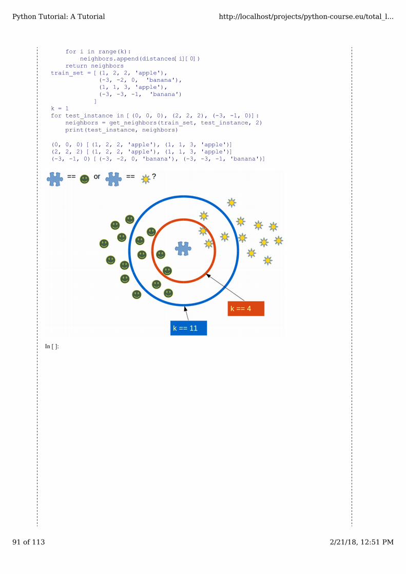
for i in range(k):neighbors.append(distances[i][0])

return neighborstrain_set = [(1, 2, 2, 'apple'),

(-3, -2, 0, 'banana'),(1, 1, 3, 'apple'),(-3, -3, -1, 'banana')]

k = 1for test_instance in [(0, 0, 0), (2, 2, 2), (-3, -1, 0)]:

neighbors = get_neighbors(train_set, test_instance, 2)print(test_instance, neighbors)

(0, 0, 0) [(1, 2, 2, 'apple'), (1, 1, 3, 'apple')](2, 2, 2) [(1, 2, 2, 'apple'), (1, 1, 3, 'apple')](-3, -1, 0) [(-3, -2, 0, 'banana'), (-3, -3, -1, 'banana')]

In [ ]:


91 of 113 2/21/18, 12:51 PM

N A I V E B AY E S C L A S S I F I E R

DEFINITION

In machine learning, a Bayes classifier is a simple probabilisticclassifier, which is based on applying Bayes' theorem. The featuremodel used by a naive Bayes classifier makes strong independenceassumptions. This means that the existence of a particular feature ofa class is independent or unrelated to the existence of every otherfeature.

Definition of independent events:

Two events E and F are independent, if both E and F have positiveprobability and if P(E|F) = P(E) and P(F|E) = P(F)

As we have stated in our definition, the Naive Bayes Classifier isbased on the Bayes' theorem. The Bayes theorem is based on theconditional probability, which we will define now:

CONDITIONAL PROBABILITY

stands for "the conditional probability of A given B", or "theprobability of A under the condition B", i.e. the probability of someevent A under the assumption that the event B took place. When in a random experiment the event B is known to haveoccurred, the possible outcomes of the experiment are reduced to B, and hence the probability of the occurrence of A ischanged from the unconditional probability into the conditional probability given B. The Joint probability is theprobability of two events in conjunction. That is, it is the probability of both events together. There are three notations forthe joint probability of A and B. It can be written as

or

The conditional probability is defined by

EXAMPLES FOR CONDITIONAL PROBABILITY

GERMAN SWISS SPEAKER

There are about 8.4 million people living in Switzerland. About 64 % of them speak German. There are about 7500million people on earth.

If some aliens randomly beam up an earthling, what are the chances that he is a German speaking Swiss?

We have the events

S: being Swiss

GS: German Speaking

The probability for a randomly chosen person to be Swiss:

If we know that somebody is Swiss, the probability of speaking German is 0.64. This corresponds to the conditionalprobability

So the probability of the earthling being Swiss and speaking German, can be calculated by the formula:

P(A|B)

P(A ∩B)

P(AB)

P(A,B)

P(A|B) =P(A ∩B)

P(B)

P(S) = = 0.001128.4

7500

P(GS|S) = 0.64

P(GS|S) =P(GS ∩ S)

P(S)


92 of 113 2/21/18, 12:51 PM

inserting the values from above gives us:

and

So our aliens end up with a chance of 0.07168 % of getting a German speaking Swiss person.

FALSE POSITIVES AND FALSE NEGATIVES

A medical research lab proposes a screening to test a large group of people for a disease. An argument against suchscreenings is the problem of false positive screening results.

Suppose 0,1% of the group suffer from the disease, and the rest is well:

and

The following is true for a screening test:

If you have the disease, the test will be positive 99% of the time, and if you don't have it, the test will be negative 99% ofthe time:

P("test positive" | "well") = 1 %

and

P("test negative" | "well") = 99 %.

Finally, suppose that when the test is applied to a person having the disease, there is a 1% chance of a false negative result(and 99% chance of getting a true positive result), i.e.

P("test negative" | "sick") = 1 %

and

P("test positive" | "sick") = 99 %

Sick Healthy Totals

Test result positive 99 999 1098

Test result negative 1 98901 98902

Totals 100 99900 100000

There are 999 False Positives and 1 False Negative.

Problem:

In many cases even medical professionals assume that "if you have this sickness, the test will be positive in 99 % of thetime and if you don't have it, the test will be negative 99 % of the time. Out of the 1098 cases that report positive resultsonly 99 (9 %) cases are correct and 999 cases are false positives (91 %), i.e. if a person gets a positive test result, theprobability that he or she actually has the disease is just about 9 %. P("sick" | "test positive") = 99 / 1098 = 9.02 %

BAYES' THEOREM

We calculated the conditional probability , which was the probability that a person speaks German, if he or she isknown to be Swiss. To calculate this we used the following equation:

What about calculating the probability , i.e. the probability that somebody is Swiss under the assumption that theperson speeks German?

0.64 =P(GS ∩ S)

0.00112

P(GS ∩ S) = 0.0007168

P(" sick ") = 0, 1

P(" well ") = 99, 9

P(GS|S)

P(GS|S) =P(GS,S)

P(S)

P(S|GS)


93 of 113 2/21/18, 12:51 PM

The equation looks like this:

Let's isolate on both equations :

As the left sides are equal, the right sides have to be equal as well:

This equation can be transformed into:

The result corresponts to Bayes' theorem

To solve our problem, - i.e. the probability that a person is Swiss, if we know that he or she speaks German - all we haveto do is calculate the right side. We know already from our previous exercise that

and

The number of German native speakers in the world corresponds to 101 millions, so we know that

Finally, we can calculate by substituting the values in our equation:

There are about 8.4 million people living in Switzerland. About 64 % of them speak German. There are about 7500million people on earth.

If the some aliens randomly beam up an earthling, what are the chances that he is a German speaking Swiss?

We have the events

: being Swiss : German Speaking

is the conditional probability of , given (posterior probability), is the prior probability of and the priorprobability of . is the conditional probability of given , called the likely-hood.

An advantage of the naive Bayes classifier is that it requires only a small amount of training data to estimate theparameters necessary for classification. Because independent variables are assumed, only the variances of the variablesfor each class need to be determined and not the entire covariance matrix.

P(S|GS) =P(GS,S)

P(GS)

P(GS,S)

P(GS,S) = P(GS|S)P(S)P(GS,S) = P(S|GS)P(GS)

P(GS|S) ∗ P(S) = P(S|GS)P(GS)

P(S|GS) =P(GS|S)P(S)

P(GS)

P(GS|S) = 0.64

P(S) = 0.00112

P(GS) = = 0.01346671017500

P(S|GS)

P(S|GS) = = = 0.0532276P(GS|S)P(S)

P(GS)0.64 ∗ 0.00112

0.0134667

S GS

P(S) = = 0.001128.4

7500

P(A|B) =P(B|A)P(A)

P(B)

P(A|B) A B P(B) B P(A)

A P(B|A) B A


94 of 113 2/21/18, 12:51 PM

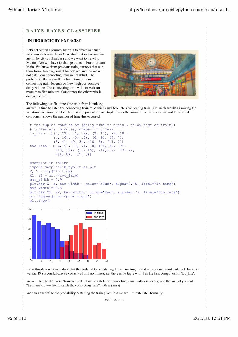
N A I V E B AY E S C L A S S I F I E R

INTRODUCTORY EXERCISE

Let's set out on a journey by train to create our firstvery simple Naive Bayes Classifier. Let us assume weare in the city of Hamburg and we want to travel toMunich. We will have to change trains in Frankfurt amMain. We know from previous train journeys that ourtrain from Hamburg might be delayed and the we willnot catch our connecting train in Frankfurt. Theprobability that we will not be in time for ourconnecting train depends on how high our possibledelay will be. The connecting train will not wait formore than five minutes. Sometimes the other train isdelayed as well.

The following lists 'in_time' (the train from Hamburgarrived in time to catch the connecting train to Munich) and 'too_late' (connecting train is missed) are data showing thesituation over some weeks. The first component of each tuple shows the minutes the train was late and the secondcomponent shows the number of time this occurred.

# the tuples consist of (delay time of train1, delay time of train2)# tuples are (minutes, number of times)in_time = [(0, 22), (1, 19), (2, 17), (3, 18),

(4, 16), (5, 15), (6, 9), (7, 7),(8, 4), (9, 3), (10, 3), (11, 2)]

too_late = [(6, 6), (7, 9), (8, 12), (9, 17),(10, 18), (11, 15), (12,16), (13, 7),(14, 8), (15, 5)]

%matplotlib inlineimport matplotlib.pyplot as pltX, Y = zip(*in_time)X2, Y2 = zip(*too_late)bar_width = 0.9plt.bar(X, Y, bar_width, color="blue", alpha=0.75, label="in time")bar_width = 0.8plt.bar(X2, Y2, bar_width, color="red", alpha=0.75, label="too late")plt.legend(loc='upper right')plt.show()

From this data we can deduce that the probability of catching the connecting train if we are one minute late is 1, becausewe had 19 successful cases experienced and no misses, i.e. there is no tuple with 1 as the first component in 'too_late'.

We will denote the event "train arrived in time to catch the connecting train" with (success) and the 'unlucky' event"train arrived too late to catch the connecting train" with (miss)

We can now define the probability "catching the train given that we are 1 minute late" formally:

S

M

P(S|1) = 19/19 = 1


95 of 113 2/21/18, 12:51 PM

We used the fact that the tuple is in 'in_time' and there is no tuple with the first component 1 in 'too_late'

It's getting critical for catching the connecting train to Munich, if we are 6 minutes late. Yet, the chances are still 60 %:

Accordingly, the probability for missing the train knowing that we are 6 minutes late is:

We can write a 'classifier' function, which will give the probability for catching the connecting train:

in_time_dict = dict(in_time)too_late_dict = dict(too_late)def catch_the_train(min):

s = in_time_dict.get(min, 0)if s == 0:

return 0else:

m = too_late_dict.get(min, 0)return s / (s + m)

for minutes in range(-1, 13):print(minutes, catch_the_train(minutes))

-1 00 1.01 1.02 1.03 1.04 1.05 1.06 0.67 0.43758 0.259 0.1510 0.1428571428571428511 0.1176470588235294112 0

A NAIVE BAYES CLASSIFIER EXAMPLE

GETTING THE DATA READY

We will use a file called 'person_data.txt'. It contains 100 random person data, male and female, with body sizes, weightsand gender tags.

import numpy as npgenders = ["male", "female"]persons = []with open("data/person_data.txt") as fh:

for line in fh:persons.append(line.strip().split())

firstnames = {}heights = {}for gender in genders:

firstnames[gender] = [ x[0] for x in persons if x[4]==gender]heights[gender] = [ x[2] for x in persons if x[4]==gender]heights[gender] = np.array(heights[gender], np.int)

for gender in ("female", "male"):

print(gender + ":")print(firstnames[gender][:10])print(heights[gender][:10])

female:

(1, 19)

P(S|6) = 9/9 + 6 = 0.6

P(S|6) = 6/9 + 6 = 0.4


96 of 113 2/21/18, 12:51 PM

['Stephanie', 'Cynthia', 'Katherine', 'Elizabeth', 'Carol', 'Christina', 'Beverly', 'Sharon', 'Denise', 'Rebecca'][149 174 183 138 145 161 179 162 148 196]male:['Randy', 'Jessie', 'David', 'Stephen', 'Jerry', 'Billy', 'Earl', 'Todd', 'Martin', 'Kenneth'][184 175 187 192 204 180 184 174 177 200]

Warning: There might be some confusion between a Python class and a Naive Bayes class. We try to avoid it by sayingexplicitly what is meant, whenever possible!

DESIGNING A FEATURE CLASS

We will now define a Python class "Feature" for the features, which we will use for classification later.

The Feature class needs a label, e.g. "heights" or "firstnames". If the feature values are numerical we may want to "bin"them to reduce the number of possible feature values. The heights from our persons have a huge range and we have only50 measured values for our Naive Bayes classes "male" and "female". We will bin them into ranges "130 to 134", "135 to139", "140 to 144" and so on by setting bin_width to 5. There is no way of binning the first names, so bin_width will beset to None.

The method frequency returns the number of occurrencies for a certain feature value or a binned range.

from collections import Counterimport numpy as npclass Feature:

def __init__(self, data, name=None, bin_width=None):self.name = nameself.bin_width = bin_widthif bin_width:

self.min, self.max = min(data), max(data)bins = np.arange((self.min // bin_width) * bin_width,

(self.max // bin_width) * bin_width,bin_width)

freq, bins = np.histogram(data, bins)self.freq_dict = dict(zip(bins, freq))self.freq_sum = sum(freq)

else:self.freq_dict = dict(Counter(data))self.freq_sum = sum(self.freq_dict.values())

def frequency(self, value):if self.bin_width:

value = (value // self.bin_width) * self.bin_widthif value in self.freq_dict:

return self.freq_dict[value]else:

return 0

We will create now two feature classes Feature for the height values of the person data set. One Feature class contains theheight for the Naive Bayes class "male" and one the heights for the class "female":

fts = {}for gender in genders:

fts[gender] = Feature(heights[gender], name=gender, bin_width=5)print(gender, fts[gender].freq_dict)

male {160: 5, 195: 2, 180: 5, 165: 4, 200: 3, 185: 8, 170: 6, 155: 1, 190: 8, 175: 7}female {160: 8, 130: 1, 165: 11, 135: 1, 170: 7, 140: 0, 175: 2, 145: 3, 180: 4, 150: 5, 185: 0, 155: 7}


97 of 113 2/21/18, 12:51 PM

BAR CHART OF FREQUENCY DISTRIBUTION

We printed out the frequencies of our bins, but it is a lot better to see these values dipicted in a bar chart. We will do thiswith the following code:

for gender in genders:frequencies = list(fts[gender].freq_dict.items())frequencies.sort(key=lambda x: x[1])X, Y = zip(*frequencies)color = "blue" if gender=="male" else "red"bar_width = 4 if gender=="male" else 3plt.bar(X, Y, bar_width, color=color, alpha=0.75, label=gender)

plt.legend(loc='upper right')plt.show()

We have to design now a Naive Bayes class in Python. We will call it NBclass. An NBclass contains one or more Featureclasses. The name of the NBclass will be stored in self.name.

class NBclass:

def __init__(self, name, *features):self.features = featuresself.name = name

def probability_value_given_feature(self,

feature_value,feature):

""" p_value_given_feature returns the probability p for a feature_value 'value' of the feature to occurr corresponds to P(d_i | p_j) where d_i is a feature variable of the feature i """

if feature.freq_sum == 0:return 0

else:return feature.frequency(feature_value) / feature.freq_sum

In the following code, we will create NBclasses with one feature, i.e. the height feature. We will use the Feature classes offts, which we have previously created:

cls = {}for gender in genders:

cls[gender] = NBclass(gender, fts[gender])

The final step for creating a simple Naive Bayes classifier consists in writing a class 'Classifier', which will use our classes'NBclass' and 'Feature'.

class Classifier:


98 of 113 2/21/18, 12:51 PM

def __init__(self, *nbclasses):self.nbclasses = nbclasses

def prob(self, *d, best_only=True):

nbclasses = self.nbclassesprobability_list = []for nbclass in nbclasses:

ftrs = nbclass.featuresprob = 1for i in range(len(ftrs)):

prob *= nbclass.probability_value_given_feature(d[i], ftrs[i])

probability_list.append( (prob, nbclass.name) )prob_values = [f[0] for f in probability_list]prob_sum = sum(prob_values)if prob_sum==0:

number_classes = len(self.nbclasses)pl = []for prob_element in probability_list:

pl.append( ((1 / number_classes), prob_element[1]))probability_list = pl

else:probability_list = [ (p[0] / prob_sum, p[1]) for p in

probability_list]if best_only:

return max(probability_list)else:

return probability_list

We will create a classifier with one feature class 'height'. We check it with values between 130 and 220 cm.

c = Classifier(cls["male"], cls["female"])for i in range(130, 220, 5):

print(i, c.prob(i, best_only=False))

130 [(0.0, 'male'), (1.0, 'female')]135 [(0.0, 'male'), (1.0, 'female')]140 [(0.5, 'male'), (0.5, 'female')]145 [(0.0, 'male'), (1.0, 'female')]150 [(0.0, 'male'), (1.0, 'female')]155 [(0.125, 'male'), (0.875, 'female')]160 [(0.38461538461538469, 'male'), (0.61538461538461542, 'female')]165 [(0.26666666666666666, 'male'), (0.73333333333333328, 'female')]170 [(0.46153846153846162, 'male'), (0.53846153846153855, 'female')]175 [(0.77777777777777779, 'male'), (0.22222222222222224, 'female')]180 [(0.55555555555555558, 'male'), (0.44444444444444448, 'female')]185 [(1.0, 'male'), (0.0, 'female')]190 [(1.0, 'male'), (0.0, 'female')]195 [(1.0, 'male'), (0.0, 'female')]200 [(1.0, 'male'), (0.0, 'female')]205 [(0.5, 'male'), (0.5, 'female')]210 [(0.5, 'male'), (0.5, 'female')]215 [(0.5, 'male'), (0.5, 'female')]

There are no persons - neither male nor female - in our learn set, with a body height between 140 and 144. That is thereason, our classifier can't base its result on learned data and therefore comes back with a fify-fifty result.

We can also train a classifier with our firstnames:

fts = {}cls = {}for gender in genders:

fts_names = Feature(firstnames[gender], name=gender)cls[gender] = NBclass(gender, fts_names)


99 of 113 2/21/18, 12:51 PM

c = Classifier(cls["male"], cls["female"])testnames = ['Edgar', 'Benjamin', 'Fred', 'Albert', 'Laura',

'Maria', 'Paula', 'Sharon', 'Jessie']for name in testnames:

print(name, c.prob(name))

Edgar (0.5, 'male')Benjamin (1.0, 'male')Fred (1.0, 'male')Albert (1.0, 'male')Laura (1.0, 'female')Maria (1.0, 'female')Paula (1.0, 'female')Sharon (1.0, 'female')Jessie (0.6666666666666667, 'female')

The name "Jessie" is an ambiguous name. there are about 66 boys per 100 girls with this name. We can learn from theprevious classification results that the probability for the name "Jessie" being "female" is about two-thirds, which iscalculated from our data set "person":

[person for person in persons if person[0] == "Jessie"]

We received the following result:

[['Jessie', 'Morgan', '175', '67.0', 'male'], ['Jessie', 'Bell', '165', '65', 'female'], ['Jessie', 'Washington', '159', '56', 'female'], ['Jessie', 'Davis', '174', '45', 'female'], ['Jessie', 'Johnson', '165', '30.0', 'male'], ['Jessie', 'Thomas', '168', '69', 'female']]

Jessie Washington is only 159 cm tall. If we have a look at the results of our Classifier, trained with heights, we see thatthe likelihood for a person 159 cm tall of being "female" is 0.875. So what about an unknown person called "Jessie" andbeing 159 cm tall? Is this person female or male?

To answer this question, we will train an Naive Bayes classifier with two feature classes, i.e. heights and firstnames:

cls = {}for gender in genders:

fts_heights = Feature(heights[gender], name="heights", bin_width=5)fts_names = Feature(firstnames[gender], name="names")cls[gender] = NBclass(gender, fts_names, fts_heights)

c = Classifier(cls["male"], cls["female"])for d in [("Maria", 140), ("Anthony", 200), ("Anthony", 153),

("Jessie", 188) , ("Jessie", 159), ("Jessie", 160) ]:print(d, c.prob(*d, best_only=False))

('Maria', 140) [(0.5, 'male'), (0.5, 'female')]('Anthony', 200) [(1.0, 'male'), (0.0, 'female')]('Anthony', 153) [(0.5, 'male'), (0.5, 'female')]('Jessie', 188) [(1.0, 'male'), (0.0, 'female')]('Jessie', 159) [(0.066666666666666666, 'male'), (0.93333333333333335, 'female')]('Jessie', 160) [(0.23809523809523817, 'male'), (0.76190476190476197, 'female')]

THE UNDERLYING THEORY

Our classifier from the previous example is based on the Bayes theorem:

where

P( |d) =cjP(d| )P( )cj cj

P(d)


100 of 113 2/21/18, 12:51 PM

is the probability of instance d being in class c_j, it is the result we want to calculate with our classifier

is the probability of generating the instance d, if the class is given

is the probability for the occurrence of class We didn't use it in our classifiers, because both classes in ourexample have been equally likely.

P(d) is the probability for the occurrence of an instance d It's not needed in the calculation, because it is the samefor all classes.

We had used only one feature in our previous examples, i.e. the 'height' or the name.

It's possible to define a Bayes Classifier with multiple features, e.g.

We get the following formula:

is only depending on the values of . This means that it is a constant as the values of the feature variables areknown.

In [ ]:

P( |d)cj

P(d| )cj cj

P( )cj cj

d = ( , , . . . , )d1 d2 dn

P( |d) = P( | )P( )cj1P(d)

∏i=1

n

di cj cj

1P(d)

, , . . .d1 d2 dn


101 of 113 2/21/18, 12:51 PM

N A I V E B AY E S C L A S S I F I E R W I T H S C I K I T

We have written Naive Bayes Classifiersfrom scratch in our previous chapter of ourtutorial. In this part of the tutorial onMachine Learning with Python, we want toshow you how to use ready-madeclassifiers. The module Scikit providesnaive Bayes classifiers "off the rack".

Our first example uses the "iris dataset"contained in the model to train and test theclassifier

# Gaussian Naive Bayesfrom sklearn importdatasetsfrom sklearn import metricsfrom sklearn.naive_bayesimport GaussianNB# load the iris datasetsdataset =datasets.load_iris()# fit a Naive Bayes model to the datamodel = GaussianNB()model.fit(dataset.data,dataset.target)print(model)# make predictionsexpected = dataset.targetpredicted = model.predict(dataset.data)# summarize the fit of the modelprint(metrics.classification_report(expected, predicted))print(metrics.confusion_matrix(expected, predicted))

GaussianNB() precision recall f1-score support 0 1.00 1.00 1.00 50 1 0.94 0.94 0.94 50 2 0.94 0.94 0.94 50avg / total 0.96 0.96 0.96 150[[50 0 0] [ 0 47 3] [ 0 3 47]]

We use our person data from the previous chapter of our tutorial to train another classifier in the next example:

import numpy as npdef prepare_person_dataset(fname):

genders = ["male", "female"]persons = []with open(fname) as fh:

for line in fh:persons.append(line.strip().split())

firstnames = []dataset = [] # weight and heightfor person in persons:

firstnames.append( (person[0], person[4]) )height_weight = (float(person[2]), float(person[3]))dataset.append( (height_weight, person[4]))

return datasetlearnset = prepare_person_dataset("data/person_data.txt")testset = prepare_person_dataset("data/person_data_testset.txt")print(learnset)


102 of 113 2/21/18, 12:51 PM

[((184.0, 73.0), 'male'), ((149.0, 52.0), 'female'), ((174.0, 63.0), 'female'), ((175.0, 67.0), 'male'), ((183.0, 81.0), 'female'), ((187.0, 60.0), 'male'), ((192.0, 96.0), 'male'), ((204.0, 91.0), 'male'), ((180.0, 66.0), 'male'), ((184.0, 52.0), 'male'), ((174.0, 53.0), 'male'), ((177.0, 91.0), 'male'), ((138.0, 37.0), 'female'), ((200.0, 82.0), 'male'), ((193.0, 79.0), 'male'), ((189.0, 79.0), 'male'), ((145.0, 59.0), 'female'), ((188.0, 53.0), 'male'), ((187.0, 81.0), 'male'), ((187.0, 99.0), 'male'), ((190.0, 81.0), 'male'), ((161.0, 48.0), 'female'), ((179.0, 75.0), 'female'), ((180.0, 67.0), 'male'), ((155.0, 48.0), 'male'), ((201.0, 122.0), 'male'), ((162.0, 62.0), 'female'), ((148.0, 49.0), 'female'), ((171.0, 50.0), 'male'), ((196.0, 86.0), 'female'), ((163.0, 46.0), 'female'), ((159.0, 37.0), 'female'), ((163.0, 53.0), 'male'), ((150.0, 39.0), 'female'), ((170.0, 56.0), 'female'), ((191.0, 55.0), 'male'), ((175.0, 37.0), 'male'), ((169.0, 78.0), 'female'), ((167.0, 59.0), 'female'), ((170.0, 78.0), 'male'), ((178.0, 79.0), 'male'), ((168.0, 71.0), 'female'), ((170.0, 37.0), 'female'), ((167.0, 58.0), 'female'), ((152.0, 43.0), 'female'), ((191.0, 81.0), 'male'), ((155.0, 48.0), 'female'), ((176.0, 61.0), 'male'), ((151.0, 41.0), 'female'), ((166.0, 59.0), 'female'), ((168.0, 46.0), 'male'), ((165.0, 65.0), 'female'), ((169.0, 67.0), 'male'), ((158.0, 43.0), 'female'), ((173.0, 61.0), 'male'), ((180.0, 74.0), 'male'), ((212.0, 59.0), 'male'), ((152.0, 62.0), 'female'), ((189.0, 67.0), 'male'), ((159.0, 56.0), 'female'), ((163.0, 58.0), 'female'), ((174.0, 45.0), 'female'), ((174.0, 69.0), 'male'), ((167.0, 47.0), 'male'), ((131.0, 37.0), 'female'), ((154.0, 74.0), 'female'), ((159.0, 59.0), 'female'), ((159.0, 58.0), 'female'), ((177.0, 83.0), 'female'), ((193.0, 96.0), 'male'), ((180.0, 83.0), 'female'), ((164.0, 54.0), 'male'), ((164.0, 64.0), 'female'), ((171.0, 52.0), 'male'), ((163.0, 41.0), 'female'), ((165.0, 30.0), 'male'), ((161.0, 61.0), 'female'), ((198.0, 75.0), 'male'), ((183.0, 70.0), 'female'), ((185.0, 71.0), 'male'), ((175.0, 58.0), 'male'), ((195.0, 89.0), 'male'), ((170.0, 66.0), 'female'), ((167.0, 61.0), 'female'), ((166.0, 65.0), 'female'), ((180.0, 88.0), 'female'), ((164.0, 55.0), 'male'), ((161.0, 53.0), 'female'), ((187.0, 76.0), 'male'), ((170.0, 63.0), 'female'), ((192.0, 101.0), 'male'), ((175.0, 56.0), 'male'), ((190.0, 100.0), 'male'), ((164.0, 63.0), 'male'), ((172.0, 61.0), 'female'), ((168.0, 69.0), 'female'), ((156.0, 51.0), 'female'), ((167.0, 40.0), 'female'), ((161.0, 18.0), 'male'), ((167.0, 56.0), 'female')]

# Gaussian Naive Bayesfrom sklearn import datasetsfrom sklearn import metricsfrom sklearn.naive_bayes import GaussianNBmodel = GaussianNB()#print(dataset.data, dataset.target)w, l = zip(*learnset)w = np.array(w)l = np.array(l)model.fit(w, l)print(model)w, l = zip(*testset)w = np.array(w)l = np.array(l)predicted = model.predict(w)print(predicted)print(l)# summarize the fit of the modelprint(metrics.classification_report(l, predicted))print(metrics.confusion_matrix(l, predicted))

GaussianNB()['female' 'male' 'male' 'female' 'female' 'male' 'female' 'female' 'female' 'female' 'female' 'female' 'female' 'female' 'male' 'female' 'male' 'female' 'female' 'female' 'male' 'female' 'female' 'male' 'male' 'female' 'female' 'male' 'male' 'male' 'female' 'female' 'male' 'male' 'male' 'female' 'female' 'male' 'female' 'male' 'male' 'female' 'female' 'male' 'female' 'male' 'male' 'female' 'male' 'female' 'female' 'female' 'male' 'female' 'female' 'male' 'female' 'female' 'male' 'female' 'female' 'male' 'female' 'female' 'female' 'female' 'male' 'female' 'female' 'female'


103 of 113 2/21/18, 12:51 PM

'female' 'female' 'male' 'male' 'female' 'female' 'male' 'male' 'female' 'female' 'male' 'male' 'female' 'male' 'male' 'male' 'female' 'male' 'female' 'female' 'male' 'male' 'female' 'male' 'female' 'female' 'female' 'male' 'female' 'male']['female' 'male' 'male' 'female' 'female' 'male' 'male' 'male' 'female' 'female' 'female' 'female' 'female' 'female' 'male' 'male' 'male' 'female' 'female' 'female' 'male' 'female' 'female' 'male' 'male' 'female' 'male' 'female' 'male' 'female' 'male' 'male' 'male' 'male' 'female' 'female' 'female' 'male' 'male' 'female' 'male' 'female' 'male' 'male' 'female' 'male' 'female' 'male' 'female' 'female' 'female' 'male' 'male' 'male' 'male' 'male' 'female' 'male' 'male' 'female' 'female' 'female' 'male' 'female' 'male' 'female' 'male' 'female' 'male' 'female' 'female' 'female' 'male' 'male' 'male' 'female' 'male' 'male' 'female' 'female' 'male' 'male' 'female' 'female' 'male' 'male' 'female' 'male' 'female' 'male' 'male' 'female' 'female' 'male' 'male' 'female' 'female' 'male' 'female' 'female'] precision recall f1-score support female 0.68 0.80 0.73 50 male 0.76 0.62 0.68 50avg / total 0.72 0.71 0.71 100[[40 10] [19 31]]

In [ ]:

In [ ]:


104 of 113 2/21/18, 12:51 PM

T E X T C A T E G O R I Z A T I O N A N D C L A S S I F I C A T I O N

INTRODUCTION

Document classification/categorization is a topic ininformation science, a science dealing with the collection,analysis, classification, categorization, manipulation,retrieval, storage and propagation of information.

This might sound very abstract, but there are lots of situationsnowadays, where companies are in need of automaticclassification or categorization of documents. Just think abouta large company with thousands of incoming mail pieces perday, both electronic or paper based. Lot's of these mail piecesare without specific addressee names or departments.Somebody has to read these texts and has to decide what kindof a letter it is ("change of address", "complaints letter","inquiry about products", and so on) and to whom the document should be proceeded. This "somebody" can be anautomated text classification system.

Automated text classification, also calledcategorization of texts, has a history, whichdates back to the beginning of the 1960s. Butthe incredible increase in available onlinedocuments in the last two decades, due to theexpanding internet, has intensified andrenewed the interest in automated documentclassification and data mining. In thebeginning text classification focussed onheuristic methods, i.e. solving the task byapplying a set of rules based on expertknowledge. This approach proved to be highlyinefficient, so nowadays the focus has turnedto fully automatic learning and clusteringmethods.

The task of text classification consists in assigning a document to one or more categories, based on the semantic contentof the document. Document (or text) classification runs in two modes:

The training phase and theprediction (or classification) phase.

The training phase can be divided into three kinds:

supervised document classification is performed by an external mechanism, usually human feedback, whichprovides the necessary information for the correct classification of documents,semi-supervised document classification, a mixture between supervised and unsupervised classification: somedocuments or parts of documents are labelled by external assistance,unsupervised document classification is entirely executed without reference to external information.

We will implement a text classifier in Python using Naive Bayes. Naive Bayes is the most commonly used text classifierand it is the focus of research in text classification. A Naive Bayes classifier is based on the application of Bayes' theoremwith strong independence assumptions. "Strong independence" means: the presence or absence of a particular feature of aclass is unrelated to the presence or absence of any other feature. Naive Bayes is well suited for multiclass textclassification.

FORMAL DEFINITION

Let C = { c1, c2, ... cm} be a set of categories (classes) and D = { d1, d2, ... dn} a set of documents.

The task of the text classification consists in assigning to each pair ( ci, dj ) of C x D (with 1 ≤ i ≤ m and 1 ≤ j ≤ n) a valueof 0 or 1, i.e. the value 0, if the document dj doesn't belong to ci


105 of 113 2/21/18, 12:51 PM

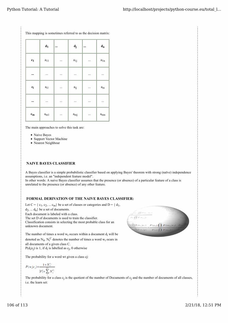
This mapping is sometimes referred to as the decision matrix:

d1 ... dj ... dn

c1 a11 ... a1j ... a1n

... ... ... ... ... ...

ci ai1 ... aij ... ain

... ... ... ... ... ...

cm am1 ... amj ... amn

The main approaches to solve this task are:

Naive BayesSupport Vector MachineNearest Neighbour

NAIVE BAYES CLASSIFIER

A Bayes classifier is a simple probabilistic classifier based on applying Bayes' theorem with strong (naïve) independenceassumptions, i.e. an "independent feature model".In other words: A naive Bayes classifier assumes that the presence (or absence) of a particular feature of a class isunrelated to the presence (or absence) of any other feature.

FORMAL DERIVATION OF THE NAIVE BAYES CLASSIFIER:

Let C = { c1, c2, ... cm} be a set of classes or categories and D = { d1,d2, ... dn} be a set of documents.Each document is labeled with a class.The set D of documents is used to train the classifier.Classification consists in selecting the most probable class for anunknown document.

The number of times a word wt occurs within a document di will be

denoted as Nit. NtC denotes the number of times a word wt ocurs in

all documents of a given class C.P(di|cj) is 1, if di is labelled as cj, 0 otherwise

The probability for a word wt given a class cj:

The probability for a class cj is the quotient of the number of Documents of cj and the number of documents of all classes,i.e. the learn set:


106 of 113 2/21/18, 12:51 PM

Finally, we come to the formula we need to classify an unknown document, i.e. the probability for a class cj given adocument di:

Unfortunately, the formula of P(c|di) we have just given is numerically not stable, because the denominator can be zerodue to rounding errors. We change this by calculating the reciprocal and reformulate the expression as a sum of stablequotients:

We can rewrite the previous formula into the following form, our final Naive Bayes classification formula, the one we willuse in our Python implementation in the following chapter:

FURTHER READING

There are lots of articles on text classification. We just name a few, which we have used for our work:

Fabrizio Sebastiani. A tutorial on automated text categorisation. In Analia Amandi and Alejandro Zunino (eds.),Proceedings of the 1st Argentinian Symposium on Artificial Intelligence (ASAI'99), Buenos Aires, AR, 1999, pp.7-35.Lewis, David D., Naive (Bayes) at Forty: The independence assumption in informal retrieval, Lecture Notes inComputer Science (1998), 1398, Issue: 1398, Publisher: Springer, Pages: 4-15K. Nigam, A. McCallum, S. Thrun and T. Mitchell, Text classification from labeled and unlabeled documents usingEM, Machine Learning 39 (2000) (2/3), pp. 103-134.


107 of 113 2/21/18, 12:51 PM

T E X T C L A S S I F I C A T I O N I N P Y T H O N

INTRODUCTION

In the previous chapter, we have deduced the formula for calculating the probabilitythat a document d belongs to a category or class c, denoted as P(c|d).

We have transformed the standard formular for P(c|d), as it is used in many treatises1,into a numerically stable form.

We use a Naive Bayes classifier for our implementation in Python. The formalintroduction into the Naive Bayes approach can be found in our previous chapter.

Python is ideal for text classification, because of it's strong string class with powerfulmethods. Furthermore the regular expression module re of Python provides the userwith tools, which are way beyond other programming languages.

The only downside might be that this Python implementation is not tuned forefficiency.

THE PYTHON IMPLEMENTATION

Warning: The implementation is in Python 3 and it is not compatible to Python 2.x!

DOCUMENT REPRESENTATION

The document representation, which is based on the bag of word model, is illustrated in the following diagram:

IMPORTS NEEDED

Our implementation needs the regular expression module re and the os module:

import re, os

BAGOFWORDS CLASS

class BagOfWords(object): """ Implementing a bag of words, words corresponding with their frequency of usages in a "document"


108 of 113 2/21/18, 12:51 PM

for usage by the Document class, DocumentClass class and the Pool class.""" def __init__(self): self.__number_of_words = 0 self.__bag_of_words = {} def __add__(self,other): """ Overloading of the "+" operator to join two BagOfWords """ erg = BagOfWords() sum = erg.__bag_of_words for key in self.__bag_of_words: sum[key] = self.__bag_of_words[key] if key in other.__bag_of_words: sum[key] += other.__bag_of_words[key] for key in other.__bag_of_words: if key not in sum: sum[key] = other.__bag_of_words[key] return erg def add_word(self,word): """ A word is added in the dictionary __bag_of_words""" self.__number_of_words += 1 if word in self.__bag_of_words: self.__bag_of_words[word] += 1 else: self.__bag_of_words[word] = 1 def len(self): """ Returning the number of different words of an object """ return len(self.__bag_of_words) def Words(self): """ Returning a list of the words contained in the object """ return self.__bag_of_words.keys() def BagOfWords(self): """ Returning the dictionary, containing the words (keys) with their frequency (values)""" return self.__bag_of_words def WordFreq(self,word): """ Returning the frequency of a word """ if word in self.__bag_of_words: return self.__bag_of_words[word] else: return 0

THE DOCUMENT CLASS

class Document(object): """ Used both for learning (training) documents and for testing documents. The optional parameter lear has to be set to True, if a classificator should be trained. If it is a test document learn has to be set to False. """ _vocabulary = BagOfWords()

def __init__(self, vocabulary): self.__name = "" self.__document_class = None self._words_and_freq = BagOfWords() Document._vocabulary = vocabulary


109 of 113 2/21/18, 12:51 PM

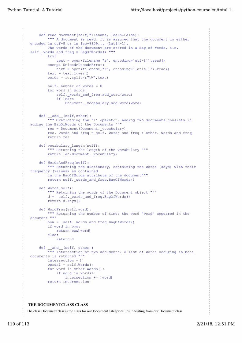
def read_document(self,filename, learn=False): """ A document is read. It is assumed that the document is either encoded in utf-8 or in iso-8859... (latin-1). The words of the document are stored in a Bag of Words, i.e. self._words_and_freq = BagOfWords() """ try: text = open(filename,"r", encoding='utf-8').read() except UnicodeDecodeError: text = open(filename,"r", encoding='latin-1').read() text = text.lower() words = re.split(r"\W",text)

self._number_of_words = 0 for word in words: self._words_and_freq.add_word(word) if learn: Document._vocabulary.add_word(word)

def __add__(self,other): """ Overloading the "+" operator. Adding two documents consists in adding the BagOfWords of the Documents """ res = Document(Document._vocabulary) res._words_and_freq = self._words_and_freq + other._words_and_freq return res def vocabulary_length(self): """ Returning the length of the vocabulary """ return len(Document._vocabulary) def WordsAndFreq(self): """ Returning the dictionary, containing the words (keys) with their frequency (values) as contained in the BagOfWords attribute of the document""" return self._words_and_freq.BagOfWords() def Words(self): """ Returning the words of the Document object """ d = self._words_and_freq.BagOfWords() return d.keys() def WordFreq(self,word): """ Returning the number of times the word "word" appeared in the document """ bow = self._words_and_freq.BagOfWords() if word in bow: return bow[word] else: return 0 def __and__(self, other): """ Intersection of two documents. A list of words occuring in both documents is returned """ intersection = [] words1 = self.Words() for word in other.Words(): if word in words1: intersection += [word] return intersection

THE DOCUMENTCLASS CLASS

The class DocumentClass is the class for our Document categories. It's inheriting from our Document class.


110 of 113 2/21/18, 12:51 PM

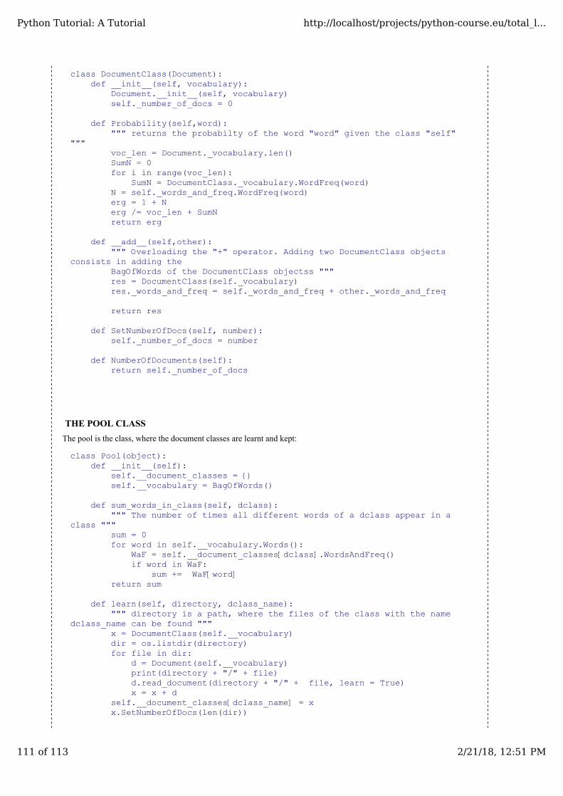
class DocumentClass(Document): def __init__(self, vocabulary): Document.__init__(self, vocabulary) self._number_of_docs = 0

def Probability(self,word): """ returns the probabilty of the word "word" given the class "self" """ voc_len = Document._vocabulary.len() SumN = 0 for i in range(voc_len): SumN = DocumentClass._vocabulary.WordFreq(word) N = self._words_and_freq.WordFreq(word) erg = 1 + N erg /= voc_len + SumN return erg

def __add__(self,other): """ Overloading the "+" operator. Adding two DocumentClass objects consists in adding the BagOfWords of the DocumentClass objectss """ res = DocumentClass(self._vocabulary) res._words_and_freq = self._words_and_freq + other._words_and_freq

return res

def SetNumberOfDocs(self, number): self._number_of_docs = number def NumberOfDocuments(self): return self._number_of_docs

THE POOL CLASS

The pool is the class, where the document classes are learnt and kept:

class Pool(object): def __init__(self): self.__document_classes = {} self.__vocabulary = BagOfWords() def sum_words_in_class(self, dclass): """ The number of times all different words of a dclass appear in a class """ sum = 0 for word in self.__vocabulary.Words(): WaF = self.__document_classes[dclass].WordsAndFreq() if word in WaF: sum += WaF[word] return sum def learn(self, directory, dclass_name): """ directory is a path, where the files of the class with the name dclass_name can be found """ x = DocumentClass(self.__vocabulary) dir = os.listdir(directory) for file in dir: d = Document(self.__vocabulary) print(directory + "/" + file) d.read_document(directory + "/" + file, learn = True) x = x + d self.__document_classes[dclass_name] = x x.SetNumberOfDocs(len(dir))


111 of 113 2/21/18, 12:51 PM

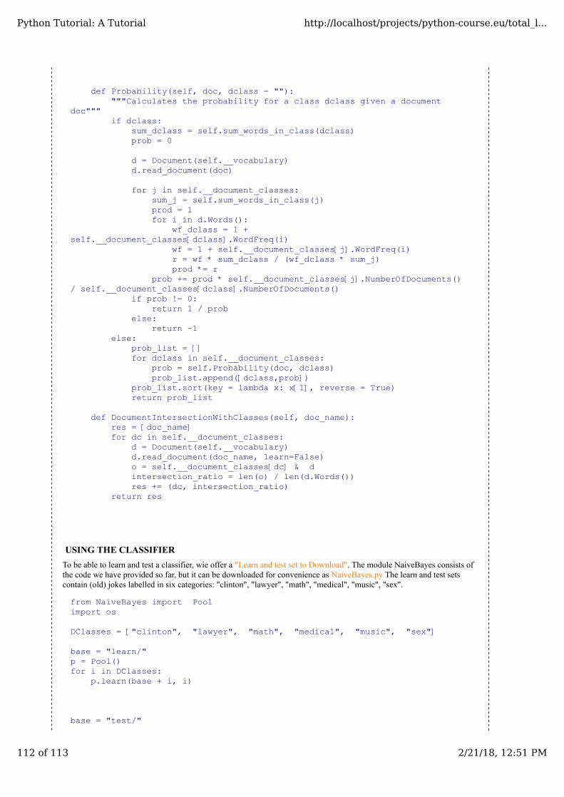
def Probability(self, doc, dclass = ""): """Calculates the probability for a class dclass given a document doc""" if dclass: sum_dclass = self.sum_words_in_class(dclass) prob = 0 d = Document(self.__vocabulary) d.read_document(doc)

for j in self.__document_classes: sum_j = self.sum_words_in_class(j) prod = 1 for i in d.Words(): wf_dclass = 1 + self.__document_classes[dclass].WordFreq(i) wf = 1 + self.__document_classes[j].WordFreq(i) r = wf * sum_dclass / (wf_dclass * sum_j) prod *= r prob += prod * self.__document_classes[j].NumberOfDocuments() / self.__document_classes[dclass].NumberOfDocuments() if prob != 0: return 1 / prob else: return -1 else: prob_list = [] for dclass in self.__document_classes: prob = self.Probability(doc, dclass) prob_list.append([dclass,prob]) prob_list.sort(key = lambda x: x[1], reverse = True) return prob_list

def DocumentIntersectionWithClasses(self, doc_name): res = [doc_name] for dc in self.__document_classes: d = Document(self.__vocabulary) d.read_document(doc_name, learn=False) o = self.__document_classes[dc] & d intersection_ratio = len(o) / len(d.Words()) res += (dc, intersection_ratio) return res

USING THE CLASSIFIER

To be able to learn and test a classifier, wie offer a "Learn and test set to Download". The module NaiveBayes consists ofthe code we have provided so far, but it can be downloaded for convenience as NaiveBayes.py The learn and test setscontain (old) jokes labelled in six categories: "clinton", "lawyer", "math", "medical", "music", "sex".

from NaiveBayes import Poolimport os

DClasses = ["clinton", "lawyer", "math", "medical", "music", "sex"]

base = "learn/"p = Pool()for i in DClasses: p.learn(base + i, i)

base = "test/"


112 of 113 2/21/18, 12:51 PM

for i in DClasses: dir = os.listdir(base + i) for file in dir: res = p.Probability(base + i + "/" + file) print(i + ": " + file + ": " + str(res))

The output of the previous program is contained in the file NaiveBayes_example_results.txt

Footnotes:1 Please see our "Further Reading" section of our previous chapter


113 of 113 2/21/18, 12:51 PM