machine learning: learning decision...

Machine Learning: Learning Decision Trees

Knut Hinkelmann

Prof. Dr. Knut Hinkelmann

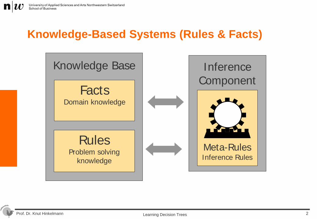
Knowledge-Based Systems (Rules & Facts)

Knowledge Base Inference Component

Facts Domain knowledge

Rules Problem solving

knowledge

Meta-Rules Inference Rules

Learning Decision Trees 2


Creating Knowledge Bases

Manual: Human expert builds rules Rules are often redundant, incomplete, inconsistent or inefficient This is also call Knowledge Engineering

Machine Learning: automatic derivation of rules from example data this is also called Data Mining or Rule Induction



What is Machine Learning?

Determine rules from data/facts

Improve performance with experience

Getting computers to program themselves

…



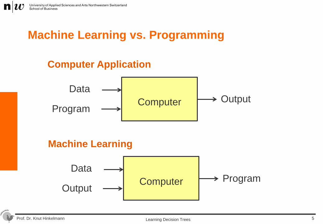
Machine Learning vs. Programming

Data

Program Output Computer

Data

Output Program Computer

Computer Application

Machine Learning



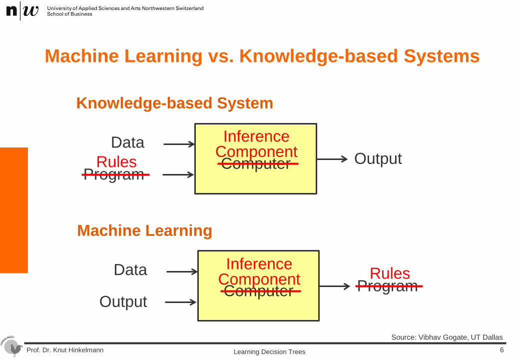
Machine Learning vs. Knowledge-based Systems

Source: Vibhav Gogate, UT Dallas

Data

Program Output Computer

Data

Output Program Computer

Knowledge-based System

Machine Learning

Rules

Rules

Inference Component

Inference Component



Types of Learning

Supervised learning Solutions/classes for examples are known Criteria for classes are learned

Unsupervised No prior knowledge classes have to be determined

Reinforcement occasional rewards



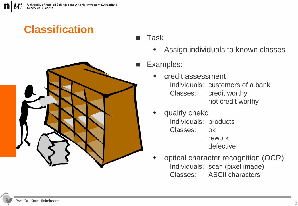
Classification Task

Assign individuals to known classes

Examples: credit assessment

Individuals: customers of a bank Classes: credit worthy

not credit worthy

quality chekc Individuals: products Classes: ok

rework defective

optical character recognition (OCR) Individuals: scan (pixel image) Classes: ASCII characters

8


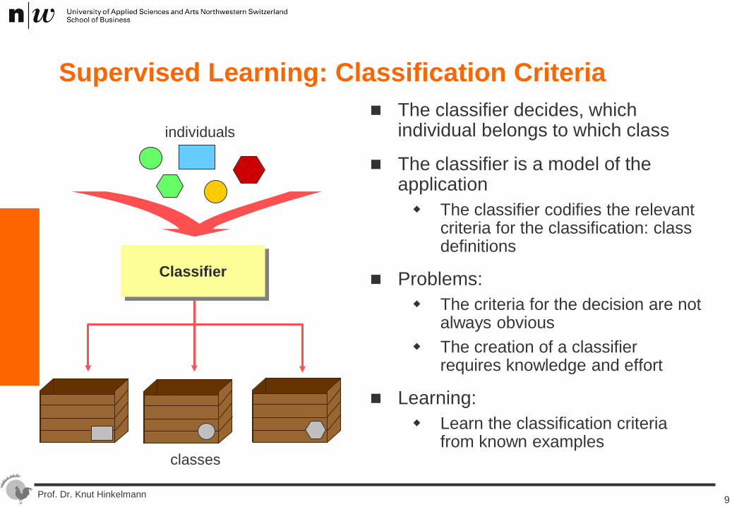
Supervised Learning: Classification Criteria The classifier decides, which

individual belongs to which class

The classifier is a model of the application The classifier codifies the relevant

criteria for the classification: class definitions

Problems: The criteria for the decision are not

always obvious The creation of a classifier

requires knowledge and effort

Learning: Learn the classification criteria

from known examples

Classifier

individuals

classes

9


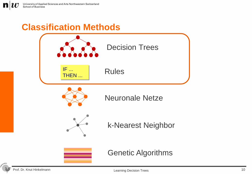
Classification Methods

Decision Trees

Neuronale Netze

Rules IF ... THEN ...

k-Nearest Neighbor

Genetic Algorithms



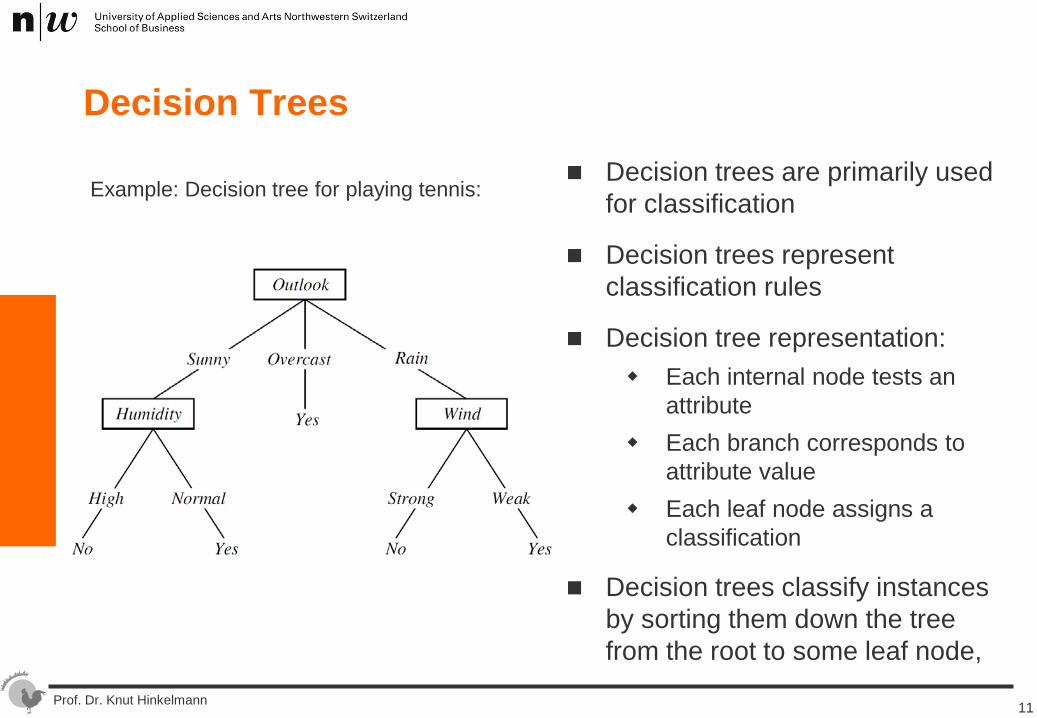
Decision Trees

Decision trees are primarily used for classification

Decision trees represent classification rules

Decision tree representation: Each internal node tests an

attribute Each branch corresponds to

attribute value Each leaf node assigns a

classification

Decision trees classify instances by sorting them down the tree from the root to some leaf node,

Example: Decision tree for playing tennis:

11


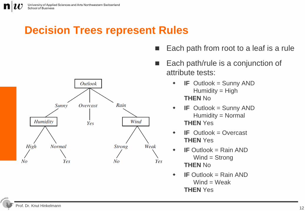
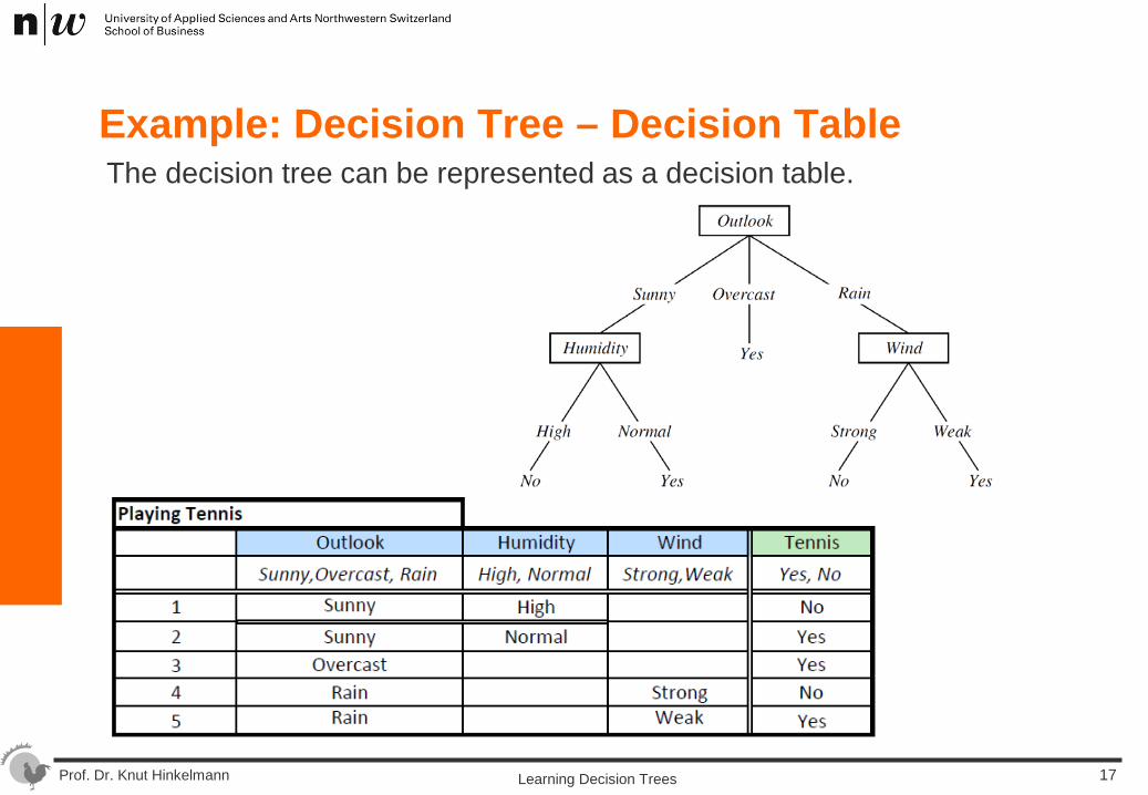
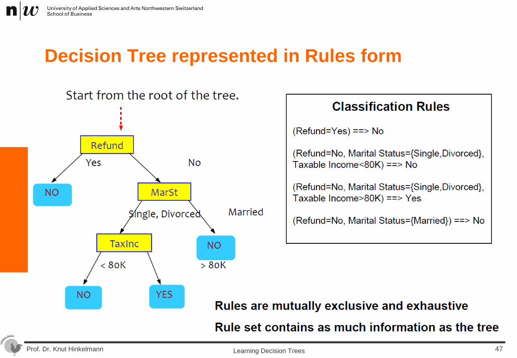
Decision Trees represent Rules Each path from root to a leaf is a rule

Each path/rule is a conjunction of attribute tests: IF Outlook = Sunny AND

Humidity = High THEN No

IF Outlook = Sunny AND Humidity = Normal THEN Yes

IF Outlook = Overcast THEN Yes

IF Outlook = Rain AND Wind = Strong THEN No

IF Outlook = Rain AND Wind = Weak THEN Yes

12


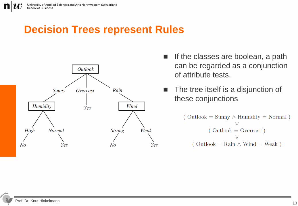
Decision Trees represent Rules

If the classes are boolean, a path can be regarded as a conjunction of attribute tests.

The tree itself is a disjunction of these conjunctions

13


Learning Decision Trees by Induction

Problem

Decision tree

Training data independent dependent ... ... ... ... ... ... ... ... ... ... ... ...

Induction

Induction = Generalisation from examples



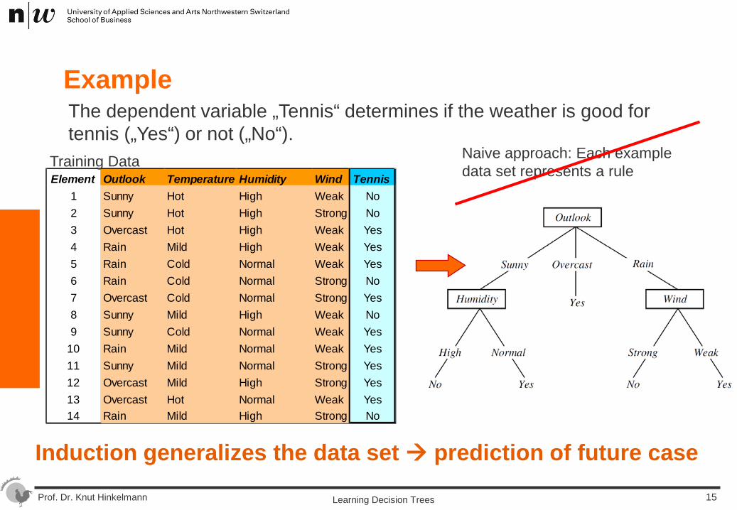
Example The dependent variable „Tennis“ determines if the weather is good for tennis („Yes“) or not („No“).

Element Outlook Temperature Humidity Wind Tennis1 Sunny Hot High Weak No2 Sunny Hot High Strong No3 Overcast Hot High Weak Yes4 Rain Mild High Weak Yes5 Rain Cold Normal Weak Yes6 Rain Cold Normal Strong No7 Overcast Cold Normal Strong Yes8 Sunny Mild High Weak No9 Sunny Cold Normal Weak Yes

10 Rain Mild Normal Weak Yes11 Sunny Mild Normal Strong Yes12 Overcast Mild High Strong Yes13 Overcast Hot Normal Weak Yes14 Rain Mild High Strong No

Training Data


Naive approach: Each example data set represents a rule

Induction generalizes the data set prediction of future case


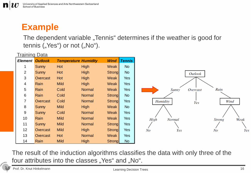
Example The dependent variable „Tennis“ determines if the weather is good for tennis („Yes“) or not („No“).

Element Outlook Temperature Humidity Wind Tennis1 Sunny Hot High Weak No2 Sunny Hot High Strong No3 Overcast Hot High Weak Yes4 Rain Mild High Weak Yes5 Rain Cold Normal Weak Yes6 Rain Cold Normal Strong No7 Overcast Cold Normal Strong Yes8 Sunny Mild High Weak No9 Sunny Cold Normal Weak Yes

10 Rain Mild Normal Weak Yes11 Sunny Mild Normal Strong Yes12 Overcast Mild High Strong Yes13 Overcast Hot Normal Weak Yes14 Rain Mild High Strong No

The result of the induction algorithms classifies the data with only three of the four attributes into the classes „Yes“ and „No“.

Training Data



Example: Decision Tree – Decision Table The decision tree can be represented as a decision table.



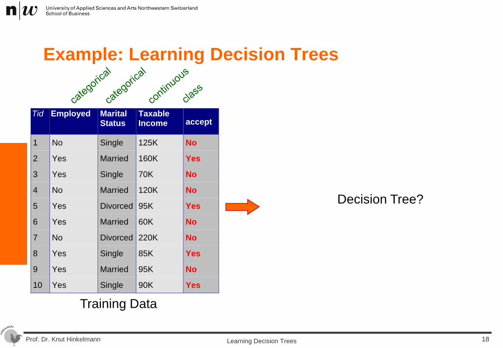
Example: Learning Decision Trees

Tid Employed Marital Status

Taxable Income accept

1 No Single 125K No

2 Yes Married 160K Yes

3 Yes Single 70K No

4 No Married 120K No

5 Yes Divorced 95K Yes

6 Yes Married 60K No

7 No Divorced 220K No

8 Yes Single 85K Yes


10 Yes Single 90K Yes 10

Training Data

Decision Tree?



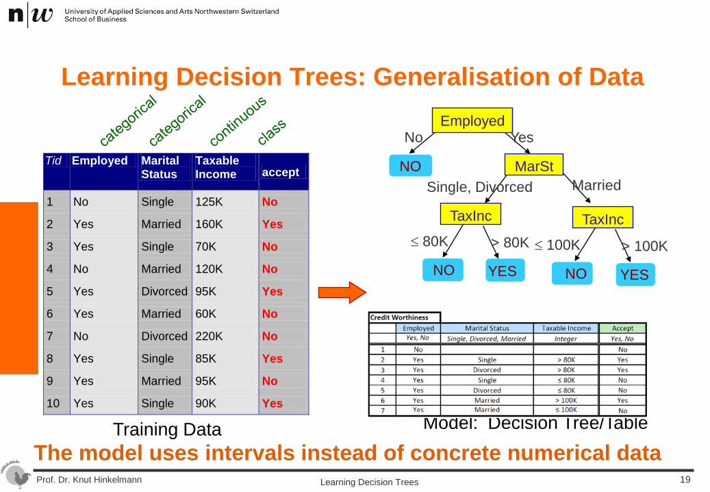
Learning Decision Trees: Generalisation of Data

Tid Employed Marital Status

Taxable Income accept

1 No Single 125K No

2 Yes Married 160K Yes

3 Yes Single 70K No

4 No Married 120K No

5 Yes Divorced 95K Yes


7 No Divorced 220K No

8 Yes Single 85K Yes


10 Yes Single 90K Yes 10

Training Data Model: Decision Tree/Table

Employed

MarSt

TaxInc

YES NO

NO

No Yes

Married Single, Divorced

≤ 80K > 80K TaxInc

YES NO

≤ 100K > 100K


The model uses intervals instead of concrete numerical data


Predictive Model for Classification

Given a collection of training records (training set) Each record consists of attributes, one of the attributes is the class The class is the dependent attribute, the other attributes are the

independent attributes

Find a model for the class attribute as a function of the values of the other attributes.

Goal: to assign a class to previously unseen records as accurately as possible.

Generalisation of data if training set does not cover all possible cases or data are too specific Induction



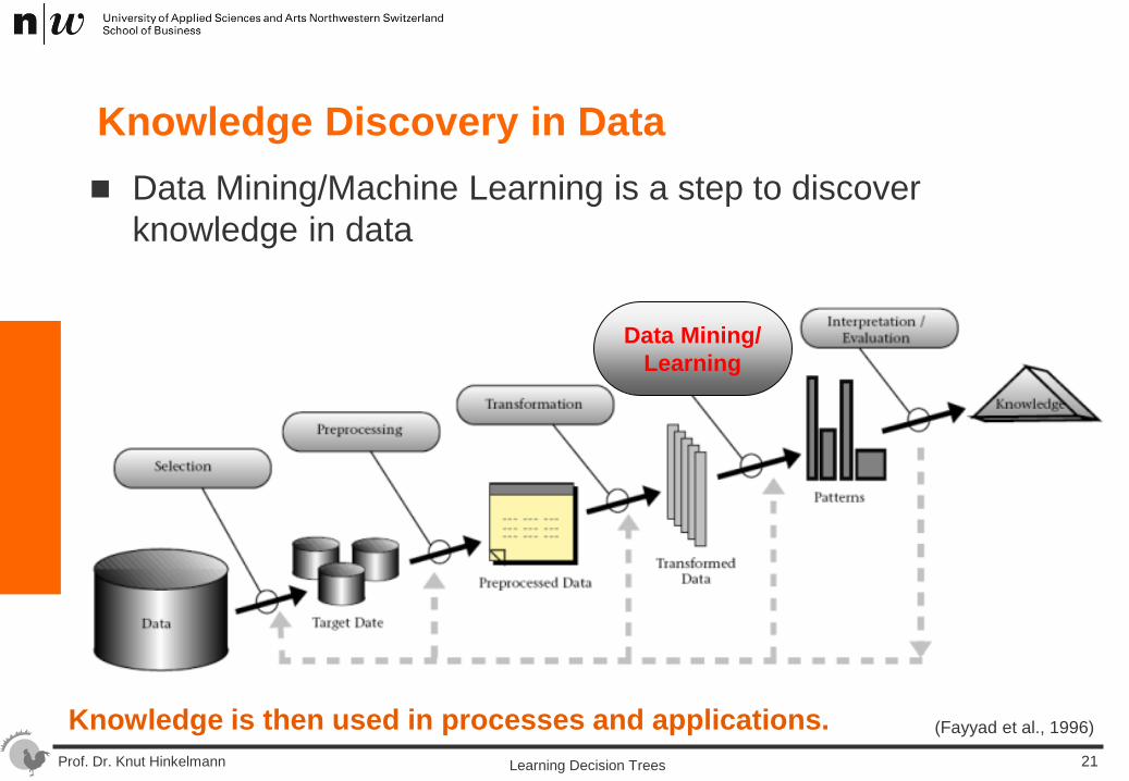
Knowledge Discovery in Data Data Mining/Machine Learning is a step to discover

knowledge in data

(Fayyad et al., 1996)

Data Mining/ Learning

Knowledge is then used in processes and applications. Learning Decision Trees 21


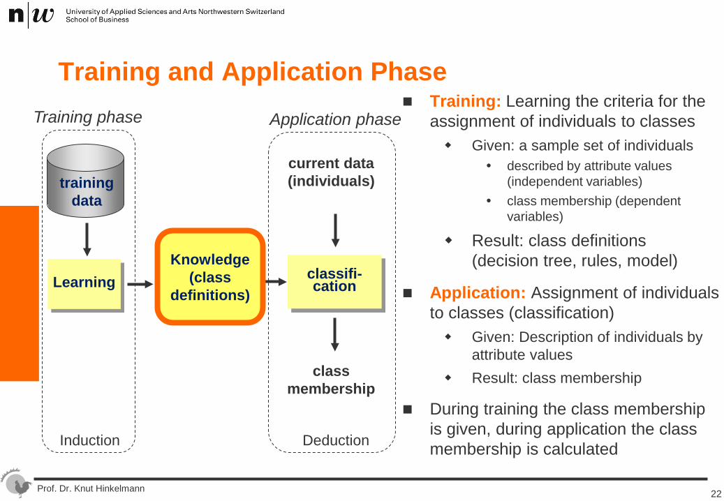
Training and Application Phase Training: Learning the criteria for the

assignment of individuals to classes Given: a sample set of individuals

described by attribute values (independent variables)

class membership (dependent variables)

Result: class definitions (decision tree, rules, model)

Application: Assignment of individuals to classes (classification) Given: Description of individuals by

attribute values Result: class membership

During training the class membership is given, during application the class membership is calculated

training data

current data (individuals)

class membership

Learning classifi-cation

Knowledge (class

definitions)

Training phase Application phase

Induction Deduction

22


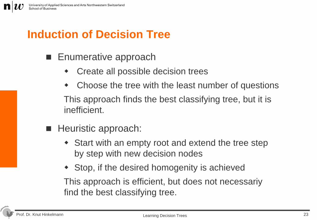
Induction of Decision Tree

Enumerative approach Create all possible decision trees Choose the tree with the least number of questions This approach finds the best classifying tree, but it is inefficient.

Heuristic approach: Start with an empty root and extend the tree step

by step with new decision nodes Stop, if the desired homogenity is achieved This approach is efficient, but does not necessariy find the best classifying tree.



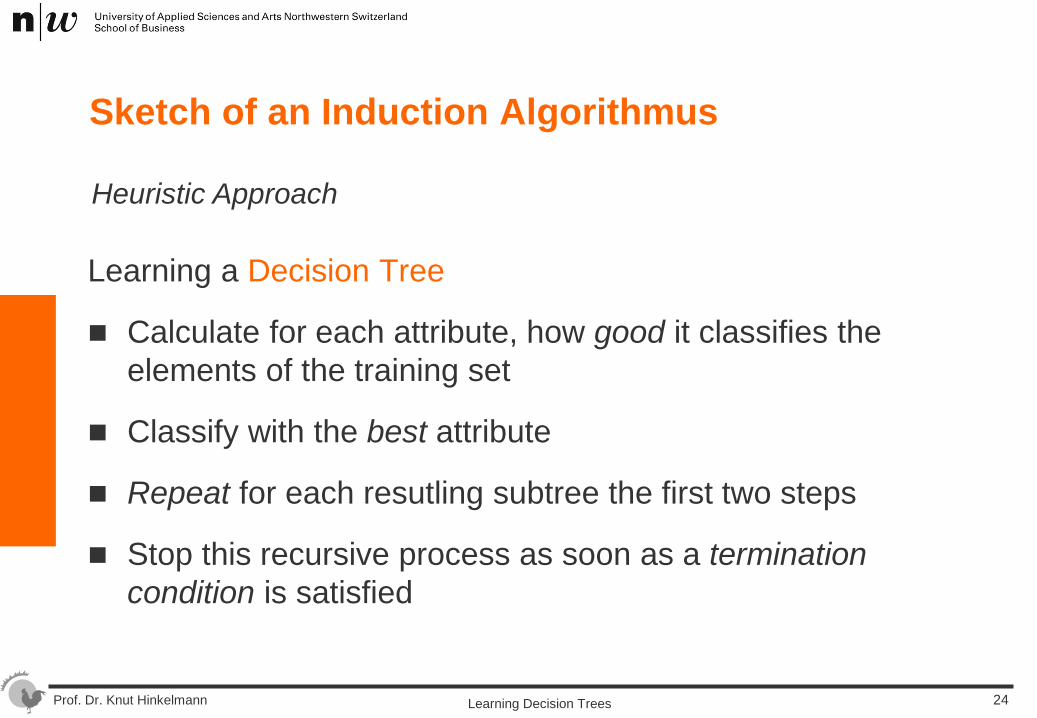
Sketch of an Induction Algorithmus

Learning a Decision Tree

Calculate for each attribute, how good it classifies the elements of the training set

Classify with the best attribute

Repeat for each resutling subtree the first two steps

Stop this recursive process as soon as a termination condition is satisfied

Heuristic Approach



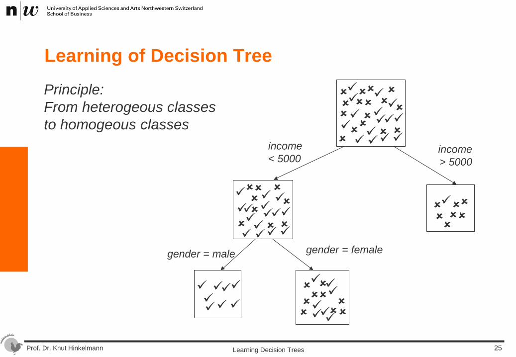
Learning of Decision Tree

Principle: From heterogeous classes to homogeous classes

income < 5000

income > 5000

gender = male gender = female



Types of Data

Discrete: endliche Zahl möglicher Werte Examples: marital status, gender Splitting: selection of values or groups of

values

Numeric infinite number of values on which an order is defined Examples: age, income Splitting: determine interval boundaries

For which kind of attributes is splitting easier?



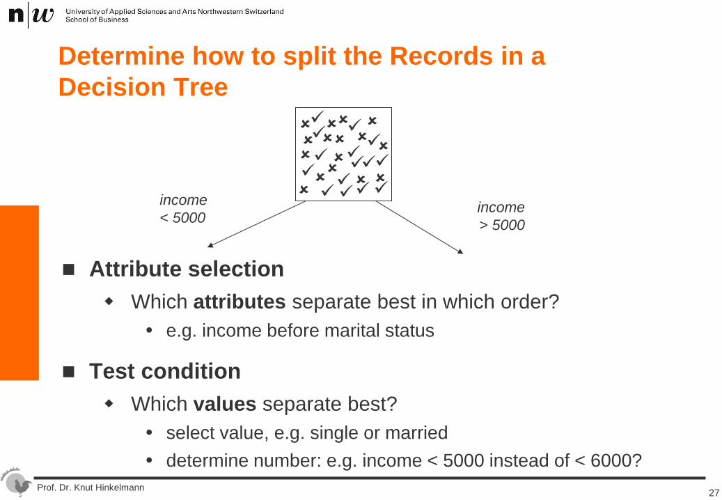
Determine how to split the Records in a Decision Tree

income < 5000

income > 5000

Attribute selection Which attributes separate best in which order?

e.g. income before marital status

Test condition Which values separate best?

select value, e.g. single or married determine number: e.g. income < 5000 instead of < 6000?

27


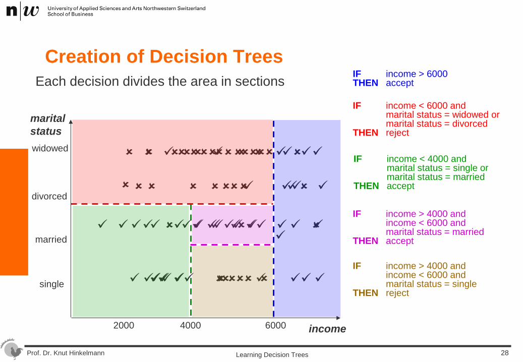
Creation of Decision Trees Each decision divides the area in sections

income

marital status widowed

2000 4000 6000

divorced

married

single

IF income > 6000 THEN accept

IF income > 4000 and income < 6000 and marital status = single THEN reject

IF income < 4000 and marital status = single or marital status = married THEN accept

IF income < 6000 and marital status = widowed or marital status = divorced THEN reject

IF income > 4000 and income < 6000 and marital status = married THEN accept



Generating Decision Trees ID3 is a basic decision learning algorithm.

It recursively selects test attributes and begins with the question "which attribute should be tested at the root of the tree? “

ID3 selects the attribute with the highest Information Gain

To calculate the information gain of an attribute one needs the Entropy of a classification the Expectation Value of the attribute



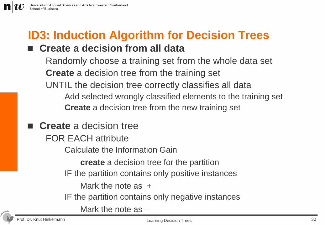
ID3: Induction Algorithm for Decision Trees Create a decision from all data

Randomly choose a training set from the whole data set Create a decision tree from the training set UNTIL the decision tree correctly classifies all data

Add selected wrongly classified elements to the training set Create a decision tree from the new training set

Create a decision tree FOR EACH attribute

Calculate the Information Gain create a decision tree for the partition

IF the partition contains only positive instances Mark the note as +

IF the partition contains only negative instances Mark the note as −



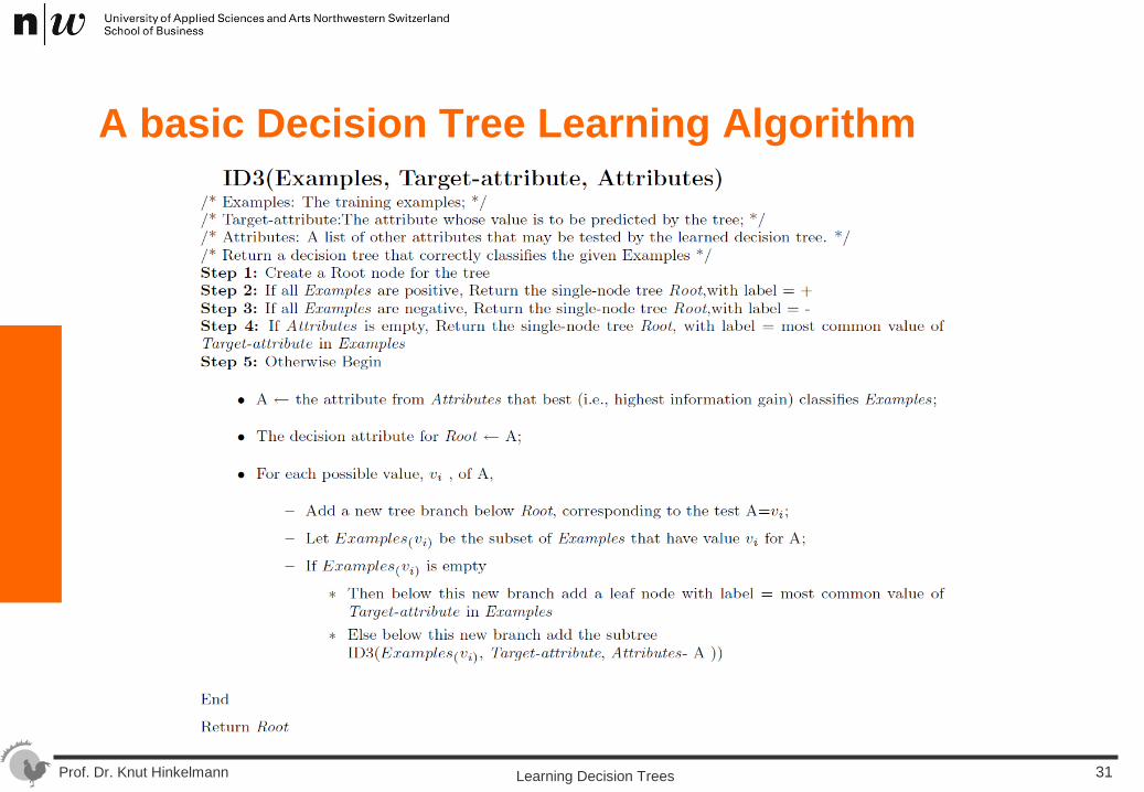
A basic Decision Tree Learning Algorithm



Entropy („disorder“)

Entropy is a measure of unpredictability of information content. The higher the information content, the lower the entropy

The more classification information a decision tree contains, the smaller the entropy

The goal of ID3 is to create a tree with minimal entropy



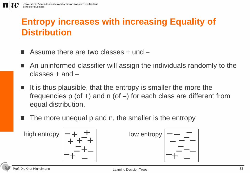
Entropy increases with increasing Equality of Distribution

Assume there are two classes + und −

An uninformed classifier will assign the individuals randomly to the classes + and −

It is thus plausible, that the entropy is smaller the more the frequencies p (of +) and n (of −) for each class are different from equal distribution.

The more unequal p and n, the smaller is the entropy

− + −

+ −

− −

−

− +

+

+ + +

high entropy

− − −

− −

− −

−

− −

+

− − −

low entropy



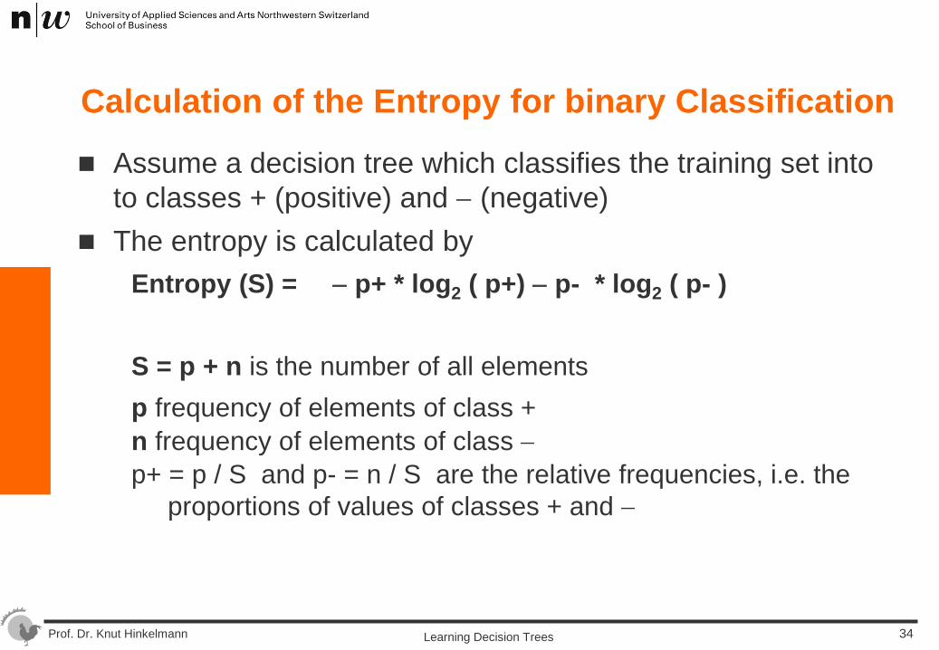
Calculation of the Entropy for binary Classification

Assume a decision tree which classifies the training set into to classes + (positive) and − (negative)

The entropy is calculated by Entropy (S) = − p+ * log2 ( p+) − p- * log2 ( p- ) S = p + n is the number of all elements p frequency of elements of class + n frequency of elements of class − p+ = p / S and p- = n / S are the relative frequencies, i.e. the

proportions of values of classes + and −



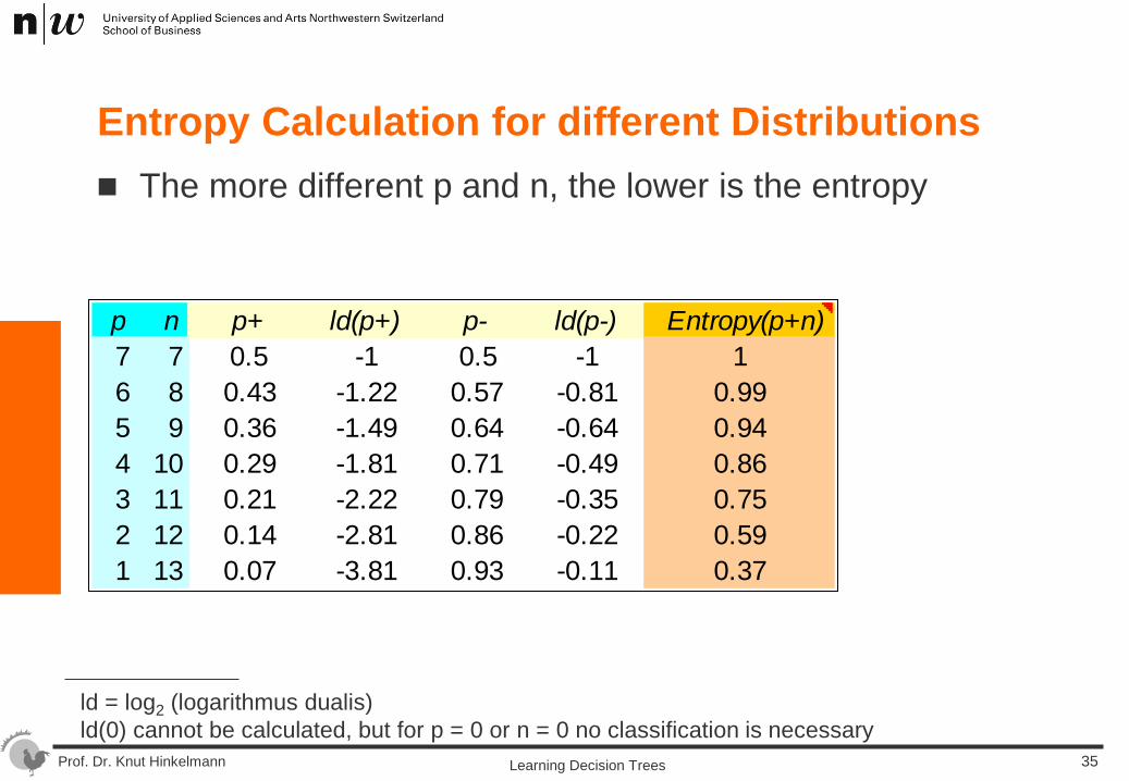
Entropy Calculation for different Distributions The more different p and n, the lower is the entropy

p n p+ ld(p+) p- ld(p-) Entropy(p+n)7 7 0.5 -1 0.5 -1 16 8 0.43 -1.22 0.57 -0.81 0.995 9 0.36 -1.49 0.64 -0.64 0.944 10 0.29 -1.81 0.71 -0.49 0.863 11 0.21 -2.22 0.79 -0.35 0.752 12 0.14 -2.81 0.86 -0.22 0.591 13 0.07 -3.81 0.93 -0.11 0.37

ld = log2 (logarithmus dualis) ld(0) cannot be calculated, but for p = 0 or n = 0 no classification is necessary



Expectation Value

The expectation value measures the

information, which is needed for

classification with attribute A



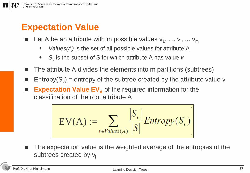
Expectation Value Let A be an attribute with m possible values v1, ..., vi, ... vm

Values(A) is the set of all possible values for attribute A Sv is the subset of S for which attribute A has value v

The attribute A divides the elements into m partitions (subtrees) Entropy(Sv) = entropy of the subtree created by the attribute value v Expectation Value EVA of the required information for the

classification of the root attribute A

The expectation value is the weighted average of the entropies of the

subtrees created by vi

EV(A) :=



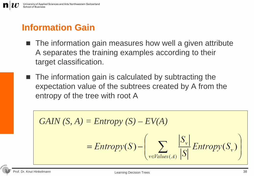
Information Gain The information gain measures how well a given attribute

A separates the training examples according to their target classification.

The information gain is calculated by subtracting the expectation value of the subtrees created by A from the entropy of the tree with root A

GAIN (S, A) = Entropy (S) – EV(A)



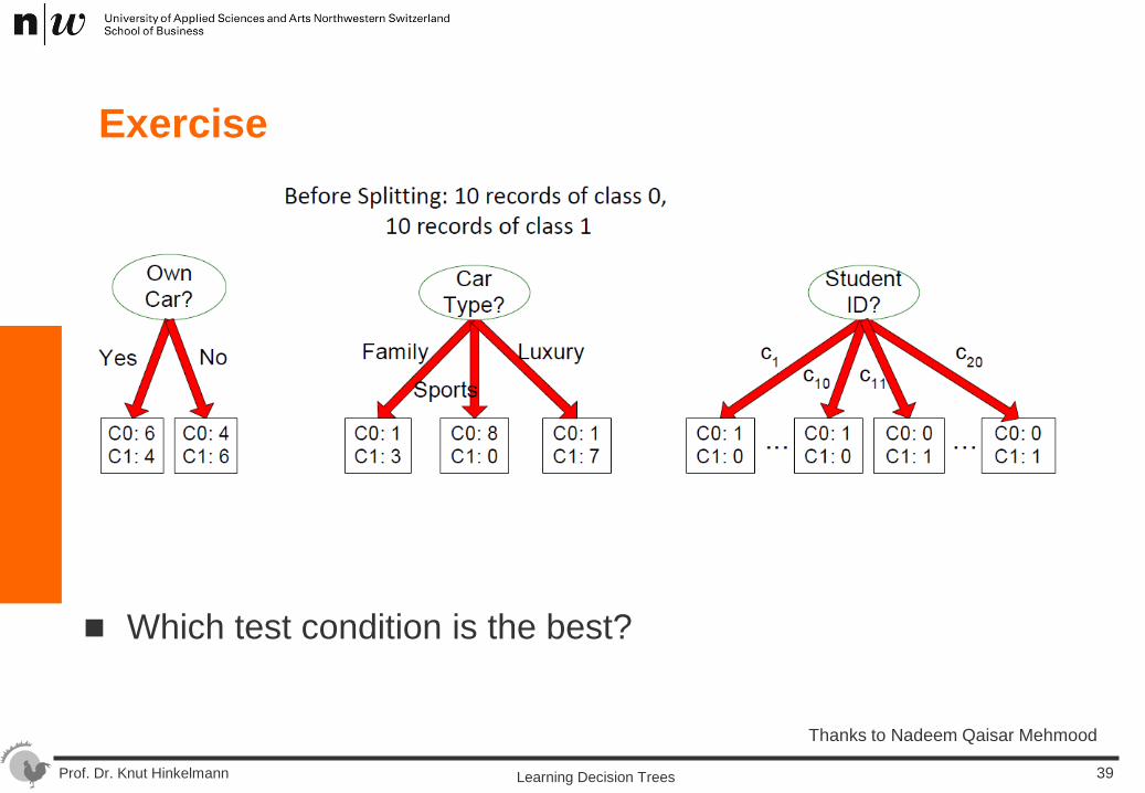
Exercise

Which test condition is the best?

Thanks to Nadeem Qaisar Mehmood



ID3: Information Gain for Attribute Selection

ID3 uses the Information Gain to select the test attribute

The recursive calculation of the attributes stops when either all partitions contain only positive or only negative elements or a user-defined threshold is achieved

On each level of the tree select the attribute

with the highest information gain



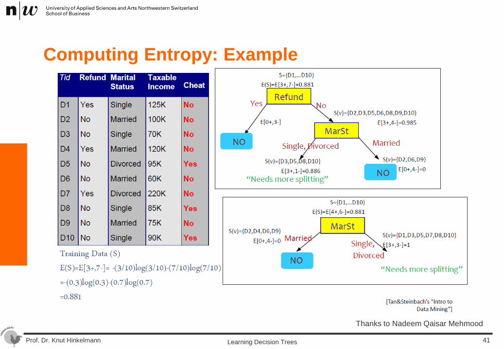
Computing Entropy: Example




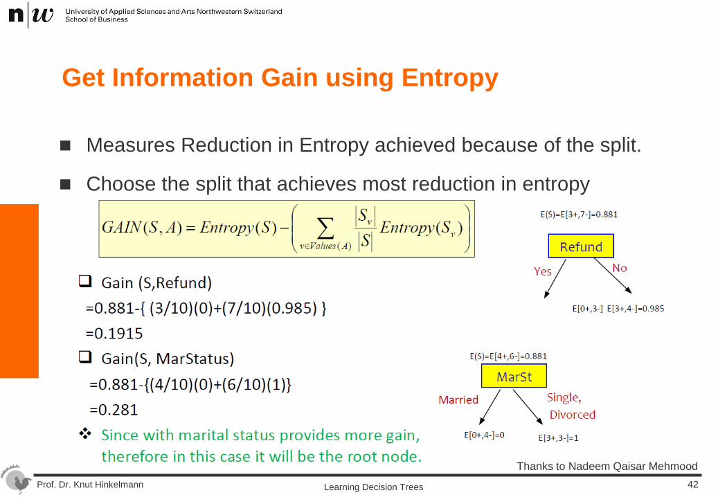
Get Information Gain using Entropy

Measures Reduction in Entropy achieved because of the split.

Choose the split that achieves most reduction in entropy




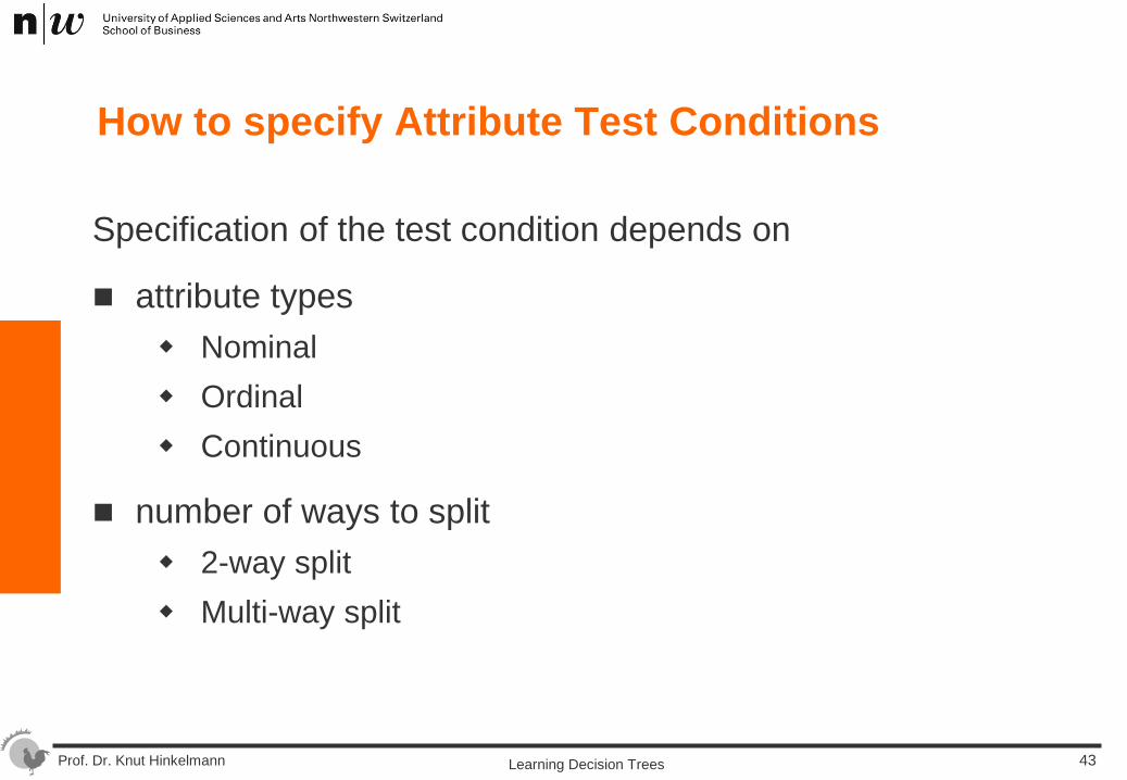
How to specify Attribute Test Conditions

Specification of the test condition depends on

attribute types Nominal Ordinal Continuous

number of ways to split 2-way split Multi-way split



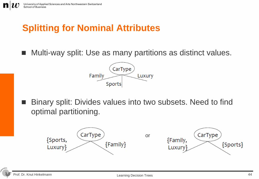
Splitting for Nominal Attributes

Multi-way split: Use as many partitions as distinct values.

Binary split: Divides values into two subsets. Need to find optimal partitioning.

or



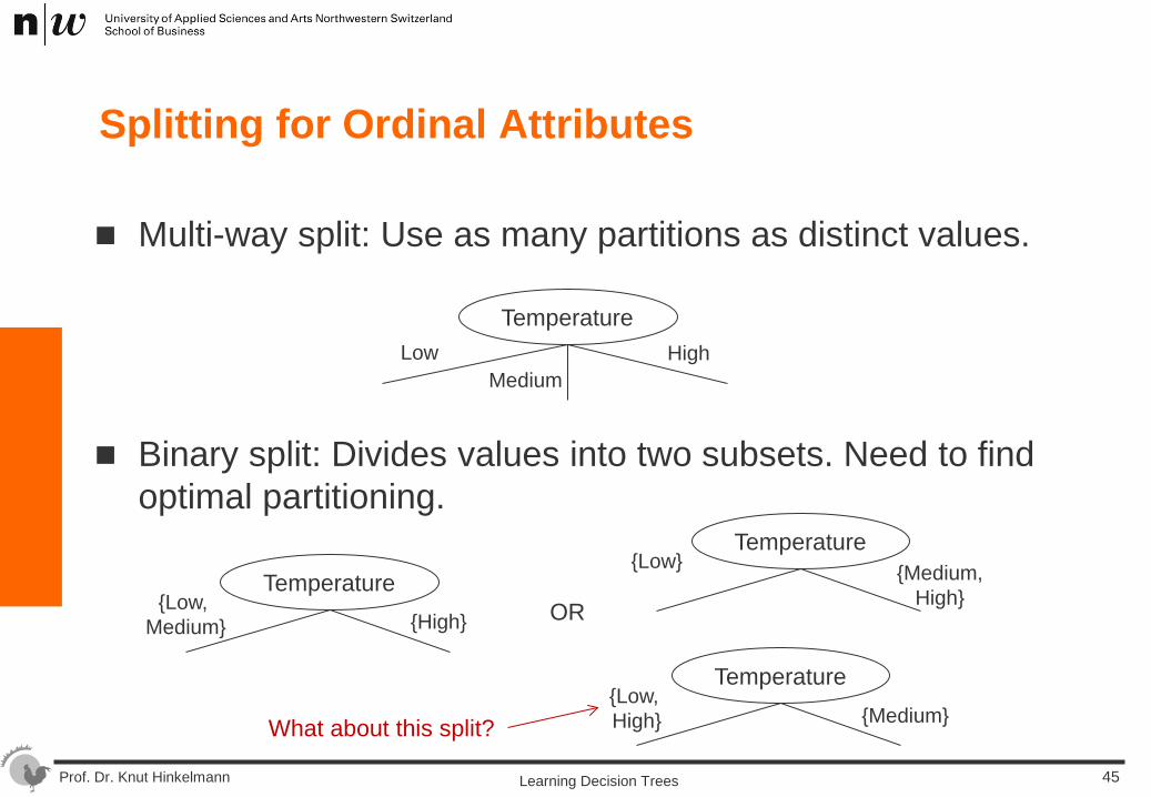
Splitting for Ordinal Attributes

Multi-way split: Use as many partitions as distinct values.

Binary split: Divides values into two subsets. Need to find optimal partitioning.

Temperature

Low Medium

High Temperature

{Low, Medium} {High}

Temperature {Low, High} {Medium}

Temperature {Low} {Medium,

High} OR

What about this split?



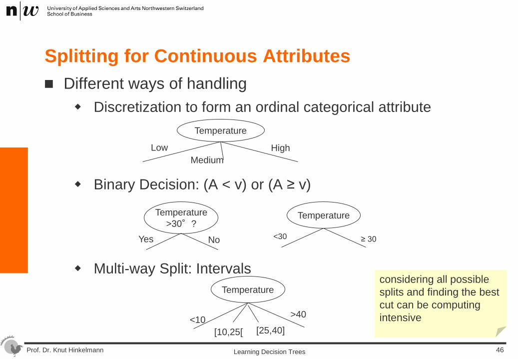
Splitting for Continuous Attributes Different ways of handling

Discretization to form an ordinal categorical attribute

Binary Decision: (A < v) or (A ≥ v)

Multi-way Split: Intervals

Temperature >30°?

Yes No

Temperature

<10 >40

[10,25[ [25,40]

Low Medium

High

Temperature

Temperature

<30 ≥ 30

considering all possible splits and finding the best cut can be computing intensive



Decision Tree represented in Rules form



Preference for Short Trees

Preference for short trees over larger trees, and for those with high information gain attributes near the root

Occam’s Razor: Prefer the simplest hypothesis that fits the data.

Arguments in favor: a short hypothesis that itts data is unlikely to be a coincidence

– compared to long hypothesis

Arguments opposed: There are many ways to define small sets of hypotheses

48 Learning Decision Trees


Overfitting

When there is noise in the data, or when the number of training examples is too small to produce a representative sample of the true target function, the rule set (hypothesis) overfits the training examples!!

Consider error of hypothesis h over training data: errortrain(h) entire distribution D of data: errorD(h)

Hypothesis h OVERFITS training data if there is an alternative hypothesis h0 such that errortrain(h) < errortrain(h0) errorD(h) > errorD(h0)

49 Learning Decision Trees


Avoiding Overfitting by Pruning

The classification quality of a tree can be improved by cutting weak branches

Reduced error pruning remove the subtree rooted at that node, make it a leaf, assign it the most common classification of the training

examples afiliated with that node.

To test accuracy, the data are separated in training set and valication set. Do until further pruning is harmful: Evaluate impact on validation set of pruning each possible node Greedily remove the one that most improves validation set accuracy



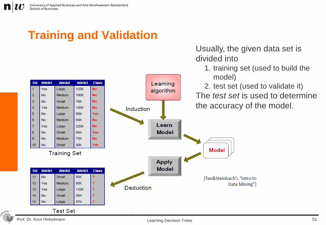
Training and Validation Usually, the given data set is divided into

1. training set (used to build the model)

2. test set (used to validate it) The test set is used to determine the accuracy of the model.



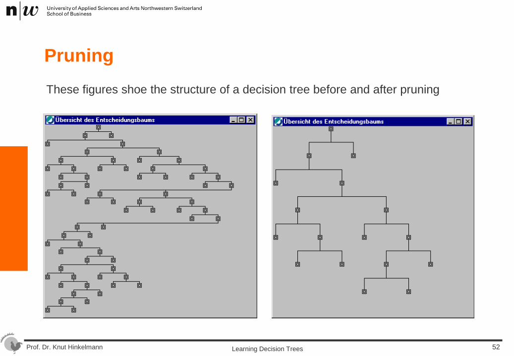
Pruning These figures shoe the structure of a decision tree before and after pruning



Generalisations Multiple Classes

Although the examples had only two classes, decision tree learning can be done also for more than two classes

Example: Quality okay, rework, defective

Probability The examples only had Boolean decisions

Example: IF income > 5000 and age > 30 THEN creditworthy

Generalisation: Probabilties for classification Example: IF income > 5000 and age > 30

THEN creditworthy with probability 0.92



Algorithms for Decision Tree Learning

Examples os algorithms for learning decision trees C4.5 (successor of ID3, predecessor of C5.0) CART (Classification and Regression Trees) CHAID (CHI-squared Automatic Interaction Detection)

A comparison 1) of various algorithms showed that the algorithms are similar with respect to classification

performance pruning increases the performance performance depends on the data and the problem.

1) D. Michie, D.J. Spiegelhalter und C.C. Taylor: Machine Learning, Neural and Statistical Classificaiton, Ellis Horwood 199


Prof. Dr. Knut Hinkelmann 55 Learning Decision Trees

Entroy (S) = 1

EV(OC) = 0.5 * E(S1) + 0.5 *E(S0)

=0.5 *(-0.6 log(0.6) – 0.4 log(0.4) + 0.5 (*(-0.4 log(0.4) – 0.6 log(0.6) = 0.97

machine learning: learning decision...

Documents