machine learning i week 14: sequence learning introduction · machine learning i week 14: sequence...
TRANSCRIPT

Machine Learning IWeek 14: Sequence Learning
Introduction
Alex Graves
Technische Universitat Munchen
29. January 2009
Alex Graves ML I – 15./16.01.2009
CogBotLabMachine Learning & Cognitive RoboticsCogBotLabMachine Learning & Cognitive Robotics
Literature
Pattern Recognition and Machine LearningChapter 13: Sequential DataChristopher M. Bishop
Machine Learning for Sequential Data: A ReviewThomas G. Dietterich, review paper
Markovian Models for Sequential DataYoshua Bengio, review paper
Supervised Sequence Labelling with Recurrent Neural NetworksAlex Graves, Ph.D. thesis
On IntelligenceJeff Hawkins
Alex Graves ML I – 15./16.01.2009
CogBotLabMachine Learning & Cognitive RoboticsCogBotLabMachine Learning & Cognitive Robotics

What is Sequence Learning?
Most machine learning algorithms are designed for independent,identically distributed (i.i.d.) data
But many interesting data types are not i.i.d.
In particular the successive points in sequential data are stronglycorrelated
Sequence learning is the study of machine learning algorithmsdesigned for sequential data. These algorithms should
1 not assume data points to be independent2 be able to deal with sequential distortions3 make use of context information
Alex Graves ML I – 15./16.01.2009
CogBotLabMachine Learning & Cognitive RoboticsCogBotLabMachine Learning & Cognitive Robotics

What is Sequence Learning Used for?
Time-Series PredictionTasks where the history of a time series is used to predict the next point.Applications include stock market prediction, weather forecasting, objecttracking, disaster prediction. . .
Sequence Labelling
Tasks where a sequence of labels is applied to a sequence of data.Applications include speech recognition, gesture recognition, proteinsecondary structure prediction, handwriting recognition. . .
For now we will concentrate on sequence labelling, but mostalgorithms are applicable to both
Alex Graves ML I – 15./16.01.2009
CogBotLabMachine Learning & Cognitive RoboticsCogBotLabMachine Learning & Cognitive Robotics

Definition of Sequence Labelling
Sequence labelling is a supervised learning task where pairs (x, t) ofinput sequences and target label sequences are used for training
The inputs x come from the set X = (Rm)∗ of sequences ofm-dimensional real-valued vectors, for some fixed m
The targets t come from the set T = L∗ of strings over the alphabetL of labels used for the task
In each pair (x, t) the target sequence is at most as long as the inputsequence: |t| ≤ |x|. They are not necessarily the same length
Definition (Sequence Labelling)
Given a training set A and a test set B, both drawn independently from afixed distribution DX×T , the goal is to use A to train an algorithmh : X 7→ T to label B in a way that minimises some task-specific errormeasure
Alex Graves ML I – 15./16.01.2009
CogBotLabMachine Learning & Cognitive RoboticsCogBotLabMachine Learning & Cognitive Robotics

Comments
We assume that the distribution DX×T that generates the data isstationary — i.e. the probability of some (x, t) ∈ DX×T remainsconstant over time (strictly speaking this does not apply to e.g.financial and weather data, because markets and climates changeover time)
Therefore the sequences (but not the individual data points) arei.i.d. This means that much of the reasoning underlying standardmachine learning algorithms also applies here, only at the level ofsequences and not points
Alex Graves ML I – 15./16.01.2009
CogBotLabMachine Learning & Cognitive RoboticsCogBotLabMachine Learning & Cognitive Robotics

Motivating Example
Online handwriting recognition is the recognition of words andletters from sequences of pen positions
The inputs are the x and y coordinates of the pen, so m is 2
The label alphabet L is just the usual Latin alphabet, possibly withextra labels for punctuation marks etc.
The error measure is the edit distance between the output of theclassifier and the target sequence
input → itput → utput → output
Alex Graves ML I – 15./16.01.2009
CogBotLabMachine Learning & Cognitive RoboticsCogBotLabMachine Learning & Cognitive Robotics
Online Handwriting with Non-Sequential Algorithms
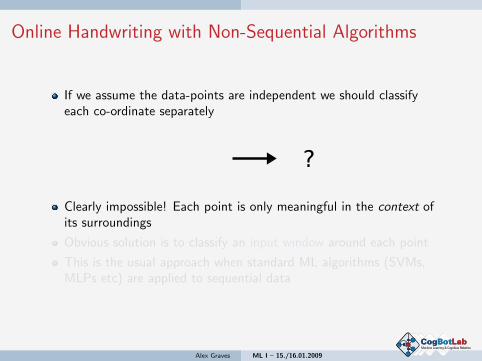
If we assume the data-points are independent we should classifyeach co-ordinate separately
Clearly impossible! Each point is only meaningful in the context ofits surroundings
Obvious solution is to classify an input window around each point
This is the usual approach when standard ML algorithms (SVMs,MLPs etc) are applied to sequential data
Alex Graves ML I – 15./16.01.2009
CogBotLabMachine Learning & Cognitive RoboticsCogBotLabMachine Learning & Cognitive Robotics

Online Handwriting with Non-Sequential Algorithms
If we assume the data-points are independent we should classifyeach co-ordinate separately
Clearly impossible! Each point is only meaningful in the context ofits surroundings
Obvious solution is to classify an input window around each point
This is the usual approach when standard ML algorithms (SVMs,MLPs etc) are applied to sequential data
Alex Graves ML I – 15./16.01.2009
CogBotLabMachine Learning & Cognitive RoboticsCogBotLabMachine Learning & Cognitive Robotics

Context and Input Windows
One problem is that it is difficult to determine in advance how bigthe window should be
Too small gives poor performance, too big is computationallyunfeasible (too many parameters)
Have to hand-tune for the dataset, depending on writing style, inputresolution etc.
Alex Graves ML I – 15./16.01.2009
CogBotLabMachine Learning & Cognitive RoboticsCogBotLabMachine Learning & Cognitive Robotics

Sequential Distortion and Input Windows
A deeper problem is that the same patterns often appear stretchedor compressed along the time axis in different sequences
In handwriting this is caused by variations in writing style
In speech it comes from variations in speaking rate, prosody etc.
Input windows are not robust to this because they ignore therelationship between the data-points. Even a 1 pixel shift looks likea completely different image!
This means poor generalisation and lots of training data needed
Alex Graves ML I – 15./16.01.2009
CogBotLabMachine Learning & Cognitive RoboticsCogBotLabMachine Learning & Cognitive Robotics
Hidden State Architectures
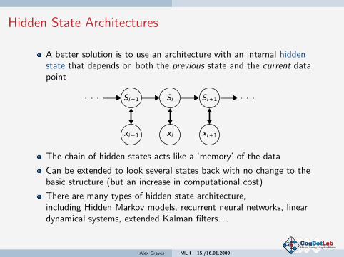
A better solution is to use an architecture with an internal hiddenstate that depends on both the previous state and the current datapoint
The chain of hidden states acts like a ‘memory’ of the data
Can be extended to look several states back with no change to thebasic structure (but an increase in computational cost)
There are many types of hidden state architecture,including Hidden Markov models, recurrent neural networks, lineardynamical systems, extended Kalman filters. . .
Alex Graves ML I – 15./16.01.2009
CogBotLabMachine Learning & Cognitive RoboticsCogBotLabMachine Learning & Cognitive Robotics

Advantages of Hidden State Architectures
Context is passed along by the ‘memory’ stored in the previousstates, so the problem of fixed-size input windows are avoided
Pr(sn|xi ) = Pr(sn|sn−1) Pr(sn−1|sn−2) . . .Pr(si |xi )
And typically require fewer parameters than input windows
Sequential distortions can be accommodated by slight changes tothe hidden state sequence. Similar sequences ‘look’ similar to thealgorithm.
The general principle is that the structure of the architecturematches the structure of the data. Put another way, hidden statearchitectures are biased towards sequential data.
Alex Graves ML I – 15./16.01.2009
CogBotLabMachine Learning & Cognitive RoboticsCogBotLabMachine Learning & Cognitive Robotics
Hidden Markov Models
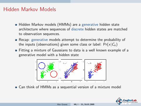
Hidden Markov models (HMMs) are a generative hidden statearchitecture where sequences of discrete hidden states are matchedto observation sequences.
Recap: generative models attempt to determine the probability ofthe inputs (observations) given some class or label: Pr(x |Ck)
Fitting a mixture of Gaussians to data is a well known example of agenerative model with a hidden state
Can think of HMMs as a sequential version of a mixture model
Alex Graves ML I – 15./16.01.2009
CogBotLabMachine Learning & Cognitive RoboticsCogBotLabMachine Learning & Cognitive Robotics

Hidden Markov Models
In a simple mixture model the observations are conditioned on thestates. This is still true for HMMs, but now the states areconditioned on the previous states as well
This creates the following joint distribution over states andobservations
Pr(x, s|θ) = Pr(s1|π)N∏
i=2
Pr(si |si−1,A)N∏
i=1
Pr(xi |si , φ)
where θ = {π,A, φ} are the HMM parameters and N is the sequencelength
Alex Graves ML I – 15./16.01.2009
CogBotLabMachine Learning & Cognitive RoboticsCogBotLabMachine Learning & Cognitive Robotics

HMM Parameters
Pr(s1 = k|π) = πk are the initial probabilities of the states
Pr(si = k|si−1 = j ,A) = Ajk is the matrix of transition probabilitiesbetween states. Note that some of its entries may be zero, since notall transitions are necessarily allowed
Pr(xi |si , φ) are the emission probabilities of the observations giventhe states. The form of Pr(xi |si , φ) depends on the task, and theperformance of HMMs depends critically on choosing a distributionable to accurately model the data. For cases where a single Gaussianis not flexible enough, mixtures of Gaussian and neural networks arecommon choices.
Pr(xi |si , φ) =n∏
k=1
aikN (xi |µi
k ,Σik)
Alex Graves ML I – 15./16.01.2009
CogBotLabMachine Learning & Cognitive RoboticsCogBotLabMachine Learning & Cognitive Robotics

Training and Using HMMs
Like most parametric models, HMMs are trained by adjusting theparameters to maximise the log-likelihood of the training data
log Pr(A|θ) =∑
(x,t)∈A
log∑
s
Pr(x, s|θ)
This can be done efficiently with the Baum-Welch algorithm
Once trained, we use the HMM to label a new data sequence x byfinding the state sequence s∗ that gives the highest joint probability
s∗ = arg maxs
p(x, s|θ).
This can be done with the Viterbi algorithm
Note: HMMs can be seen as a special case of probabilistic graphicalmodels (Bishop chapter 8). In this context Baum-Welch and Viterbiare special cases of the sum-product and max-sum algorithms.
Alex Graves ML I – 15./16.01.2009
CogBotLabMachine Learning & Cognitive RoboticsCogBotLabMachine Learning & Cognitive Robotics

Evaluation Problem
Given an observation sequence x and parameters θ what is the probabilityPr(x|θ)?
First need to compute Pr(s|θ). For example, with s = s1s2s3:
Pr(s|θ) = Pr(s1, s2, s3|θ)
= Pr(s1|θ)Pr(s2, s3 | s1, θ)
= Pr(s1|θ)Pr(s2 | s1, θ)Pr(s3 | s2, θ)
= π2A21A11A12
Then compute Pr(x|s, θ):
Pr(x | s, θ) = Pr(x1x2x3 | s1s2s3, θ)
= Pr(x1 | s1, θ)Pr(x2 | s2, θ)Pr(x3 | s3, θ) (1)
Alex Graves ML I – 15./16.01.2009
CogBotLabMachine Learning & Cognitive RoboticsCogBotLabMachine Learning & Cognitive Robotics

Evaluation Problem
Then use sum rule for probabilities to get
Pr(x|θ) =∑
s
Pr(s|θ)Pr(x|s, θ) (2)
PROBLEM: number of possible state sequences = | s |N
Alex Graves ML I – 15./16.01.2009
CogBotLabMachine Learning & Cognitive RoboticsCogBotLabMachine Learning & Cognitive Robotics

Unfold the HMM
If we unfold the state transition diagram of the above example, we obtaina lattice, or trellis, representation of the latent states. This makes iteasier to understand the following derivations.
Alex Graves ML I – 15./16.01.2009
CogBotLabMachine Learning & Cognitive RoboticsCogBotLabMachine Learning & Cognitive Robotics

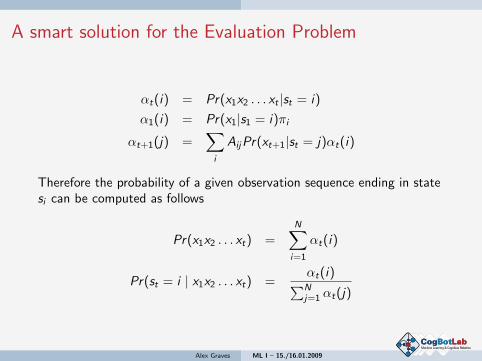
A smart solution for the Evaluation Problem
αt(i) = Pr(x1x2 . . . xt |st = i)
α1(i) = Pr(x1|s1 = i)πi
αt+1(j) =∑
i
AijPr(xt+1|st = j)αt(i)
Therefore the probability of a given observation sequence ending in statesi can be computed as follows
Pr(x1x2 . . . xt) =N∑
i=1
αt(i)
Pr(st = i | x1x2 . . . xt) =αt(i)∑Nj=1 αt(j)
Alex Graves ML I – 15./16.01.2009
CogBotLabMachine Learning & Cognitive RoboticsCogBotLabMachine Learning & Cognitive Robotics

The Viterbi Algorithm
Given an observation sequence x, which is the state sequence s with thehighest probability?
arg maxs
Pr(s|x1x2 . . . xT )
with Bayes
= arg maxs
Pr(x1x2 . . . xT | s)Pr(s)
Pr(x1x2 . . . xT )
= arg maxs
Pr(x1x2 . . . xT | s)Pr(s)
Again: Dynamic programming to the rescue!
Alex Graves ML I – 15./16.01.2009
CogBotLabMachine Learning & Cognitive RoboticsCogBotLabMachine Learning & Cognitive Robotics

The Viterbi Algorithm
The variable δt(i) is the maximum probability of
the existence of the state path s1s2 . . . st−1
ending in state i
and producing the output Pr(x1x2 . . . xt)
δt(i) = maxs1s2...st−1
Pr(s1s2 . . . st−1, st = i , x1x2 . . . xt)
Alex Graves ML I – 15./16.01.2009
CogBotLabMachine Learning & Cognitive RoboticsCogBotLabMachine Learning & Cognitive Robotics

The Viterbi Algorithm
So for any δt(j) we are looking for the most probable path of length tthat has as the last two states i and j .
But this is the most probable path (of length t − 1) to i followed by thetransition from i to j and the corresponding observation xt . Thus, themost probable path to j has i∗ as its penultimate state, with
i∗ = arg maxi
δt−1(i)AijPr(xt |st = j)
Henceδt(j) = δt−1(i∗)Ai∗jPr(xt |st = j)
Alex Graves ML I – 15./16.01.2009
CogBotLabMachine Learning & Cognitive RoboticsCogBotLabMachine Learning & Cognitive Robotics

Sequence Labelling with HMMsCould define a simple HMM with one state per labelBut for most data multi-state models are needed for each label, suchas this one used for a phoneme in speech recognition
Note that only left-to-right and self transitions are allowed. Thisensures that all observation sequences generated by the label passthrough similar ‘stages’For good performance, the states should correspond to ‘independent’observation segments within the labelCan concatenate label models to get higher level structures, such aswords
Alex Graves ML I – 15./16.01.2009
CogBotLabMachine Learning & Cognitive RoboticsCogBotLabMachine Learning & Cognitive Robotics

N-Gram Label Models
Using separate label models assumes that the observation sequencesgenerated by the labels are independent
But in practice this often isn’t true. e.g. in speech the pronunciationof a phoneme is influenced by those around it (co-articulation)
Usual solution is to use n-gram label models (e.g. triphones), withthe label generating the observations in the centre
Improves performance, but also increases the number of models(L→ Ln for L labels) and amount of training data required
Can reduce the parameter explosion by tying similar states indifferent n-grams
Alex Graves ML I – 15./16.01.2009
CogBotLabMachine Learning & Cognitive RoboticsCogBotLabMachine Learning & Cognitive Robotics

Duration Modelling
The only way an HMM can stay in the same state is by repeatedlymaking self-transitions
This means the probability of spending T timesteps in some state kdecays expontentially with T
Pr(T ) = (Akk)T (1− Akk) ∝ exp(−T ln Akk)
However this is usually an unrealistic model of state duration
One solution is to remove the self-transitions and model the durationprobability p(T |k) explicitly
When state k is entered, a value for T is first drawn from p(T |k)and T successive observations are then drawn from p(x |k)
Alex Graves ML I – 15./16.01.2009
CogBotLabMachine Learning & Cognitive RoboticsCogBotLabMachine Learning & Cognitive Robotics
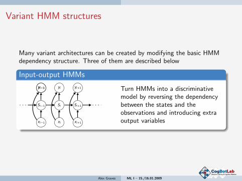
Variant HMM structures
Many variant architectures can be created by modifying the basic HMMdependency structure. Three of them are described below
Input-output HMMs
Turn HMMs into a discriminativemodel by reversing the dependencybetween the states and theobservations and introducing extraoutput variables
Alex Graves ML I – 15./16.01.2009
CogBotLabMachine Learning & Cognitive RoboticsCogBotLabMachine Learning & Cognitive Robotics

Variant HMM structures
Autoregressive HMMs
Add adding explicit dependenciesbetween the observations to improvelong-range context modelling
Factorial HMMs
Add extra chains of hidden states,thereby moving from a single-valuedto a distributed architecture andincreasing the memory capacity ofHMMs: O(log N)→ O(N)
Alex Graves ML I – 15./16.01.2009
CogBotLabMachine Learning & Cognitive RoboticsCogBotLabMachine Learning & Cognitive Robotics