(Machine) Learning from the COVID-19 Lockdown

about Electricity Market Performance with a Large

Share of Renewables

Christoph Graf∗ Federico Quaglia† Frank A. Wolak‡

October 21, 2020

Abstract

The negative demand shock due to the COVID-19 lockdown has reduced net demand

for electricity—system demand less amount of energy produced by intermittent re-

newables, hydroelectric units, and net imports—that must be served by controllable

generation units. Under normal demand conditions, introducing additional renewable

generation capacity reduces net demand. Consequently, the lockdown can provide

insights about electricity market performance with a large share of renewables. We

find that although the lockdown reduced average day-ahead prices in Italy by 45%,

re-dispatch costs increased by 73%, both relative to the average of the same magnitude

for the same period in previous years. We estimate a deep-learning model using data

from 2017–2019 and find that predicted re-dispatch costs during the lockdown period

are only 26% higher than the same period in previous years. We argue that the differ-

ence between actual and predicted lockdown period re-dispatch costs is the result of

increased opportunities for suppliers with controllable units to exercise market power

in the re-dispatch market in these persistently low net demand conditions. Our results

imply that without grid investments and other technologies to manage low net demand

conditions, an increased share of intermittent renewables is likely to increase costs of

maintaining a reliable grid.

Keywords: Net demand shock; Re-dispatch market power; Real-time grid operation;

Machine Learning; European electricity market

JEL Codes: C4; C5; D4; L9; Q4

∗Department of Economics, Stanford University, Stanford, CA 94305-6072, cgraf@stanford.edu. Financialsupport from the Austrian Science Fund (FWF), J-3917, and the Anniversary Fund of the OesterreichischeNationalbank (OeNB), 18306, is gratefully acknowledged.†Terna S.p.A., Viale Egidio Galbani, 70, 00156 Rome, Italy, federico.quaglia@terna.it.‡Program on Energy and Sustainable Development (PESD) and Department of Economics, Stanford

University, Stanford, CA 94305-6072, wolak@zia.stanford.edu.

1 Introduction

The response of governments around the world to the COVID-19 pandemic has led to nega-

tive demand shocks to almost all industries, particularly those in the energy sector. Oil-prices

plummeted and the West Texas Intermediate (WTI) futures contract for delivery in May

2020 went negative on April 20 reflecting the exhaustion of local oil storage capacity (Boren-

stein, 2020). Industrial production has halted, shops and offices were closed, and electrified

public transport operated at reduced service, all of which reduced the demand for electricity

and its pattern across time and space.

In this paper, we explore the consequences of the particularly strict lockdown in Italy

in the spring of 2020 on the performance of the country’s wholesale electricity market. The

lockdown significantly reduced the demand for controllable sources of electricity such as

thermal generation units and hydro units with storage capabilities. These units serve net

demand—the difference between system demand and supply of non-controllable sources that

include renewables such as wind, solar, non-storable hydro, and net imports.1

Consequently, the negative COVID-19 electricity demand shock translates into a negative

net demand shock because the supply of non-controllable sources were largely unchanged

during the lockdown. Therefore, lockdowns and their associated low net demand realizations

can provide insight into the challenges system operators may face as regions increase the share

of intermittent renewables in their electricity supply industries. In this sense, the COVID-19

lockdown provides a unique opportunity to analyze potential weaknesses of current electricity

market designs with a higher share of intermittent renewables envisioned by the climate

policy goals of many countries around the world.2

1Because renewables have a close to zero variable cost of producing energy, these resources will be almostalways operated when the underlying resource is available. Net-imports are deemed to be firm after the day-ahead market-clearing and are therefore another fixed source of supply for system operators to deal with inthe real-time re-dispatch process. Transmission system operators in Europe do have the ability to change netimports close to real-time but only in extreme situations to solve real-time security issues. New Europeanplatforms for trading balancing resources closer to real-time are also currently under consideration.

2Because of the intermittency of wind and solar energy production, an increase in wind and solar gen-eration capacity is likely to lead to a more volatile net demand than the equivalent average net demandreduction due to the lockdown demand reduction.

1

A back of envelope calculation reveals that the 20% decrease in business-as-usual (BAU)

demand caused by the lockdown in Italy is the equivalent to a 2.3 times higher output from

wind and solar energy at pre-COVID-19 demand levels.3 More than doubling the output from

wind and solar may sound overly ambitious but it is well within the targets for renewable

energy production in many countries around the world.

Intermittent renewables such as wind and solar, are likely to concentrate their production

within certain hours of the day, month, or year, which can significantly exacerbate the

re-dispatch cost increase we identify.4 From an environmental perspective, the first-order

effect of additional renewable capacity is that emissions will decrease because generation

from thermal units will be displaced. However, the intermittent nature of many renewable

technologies is likely to increase the importance of a second-order effect that causes a more

inefficient operation of remaining thermal generation units because of more start-ups and

faster ramps of these units (see e.g., Graf and Marcantonini, 2017; Kaffine et al., 2020).

The cost of additional start-ups and faster ramps associated with responding to the rapid

appearance and disappearance of wind and solar energy can scale rapidly with the amount

of renewable energy.5

A negative demand shock paired with lower input prices to produce electricity should

lead to lower electricity prices. In Figure 1, Panel (a), we show average hourly day-ahead

market electricity prices were down by 45% during the period of the lockdown compared

to BAU levels. However, in simplified electricity market designs that do not account for

intra-zonal transmission constraints and other relevant system security constraints in the

day-ahead market that exist in virtually all European countries and most wholesale markets

3Average hourly demand between March and April over the years 2017 to 2019 was 31.6 GWh andaverage hourly generation from wind and solar combined was 4.9 GWh. A 20% decrease in average demand(0.2 × 31.6 GWh = 6.32 GWh) is equivalent to an increase of hourly generation from wind and solar byfactor 2.3 to 11.22 GWh ( = 4.9 GWh + 6.32 GWh).

4For example, California produces more than double the amount of wind and solar energy in the summermonths relative to other months of the year.

5Schill et al. (2017) estimate that the overall number of start-ups would grow by 81% (costs by 119%)for Germany between 2013 and 2030 as the share of variable renewables is expected to grow from 14% to34% if no investments in more flexible technologies including storage are made.

2

outside of the United States, a re-dispatch process is necessary to adjust day-ahead market

schedules to ensure that they do not violate real-time transmission network and other system

security constraints (see, e.g., Graf et al., 2020a,b, for more details). Particularly in simplified

electricity market designs without an effective local market power mitigation mechanism in

place, this re-dispatch process is likely to become more costly as the share of intermittent

renewable resources increases because a larger share of the available controllable generation

capacity is likely to have to be adjusted in the re-dispatch process to achieve schedules that

are compatible with a secure operation of the grid.

In Figure 1, Panel (b), we show average hourly re-dispatch costs per MWh of demand up

by 108% relative to the average for the same time period in previous years, what we call the

BAU period.6 While the average BAU period re-dispatch costs per MWh of demand was

about 18% of the average day-ahead market price, it increased to 71% of the average daily

day-ahead market price during the lockdown. Furthermore, in the 20% highest re-dispatch

cost days during the lockdown, the average re-dispatch cost per MWh of demand exceeded

the average daily day-ahead market price.

The increase in re-dispatch costs during the lockdown has significantly reduced the cost

savings to final consumers due to the day-ahead market price decrease from lower net demand

during the lockdown. There are two major explanations for this result: First, this demand

shock created additional opportunities, not available to suppliers outside of the lockdown

period, to profit from the divergence between the network model used to clear the day-ahead

market and network constraints necessary to operate the grid in real-time as discussed in

Graf et al. (2020b).7 Second, this persistently low level of net demand is likely to require

6In absolute terms the re-dispatch costs are up by 73% relative to the same time period during previousyears. Figure D.1 compares the hourly average re-dispatch costs per week during the lockdown versus thesame time during previous years.

7In order to ensure a secure operation of the power system, generation units providing ancillary servicesshould be distributed throughout the transmission network. The probability that the schedules that emergefrom the day-ahead market meet this requirement decreases when a lower number of power plants aredispatched due to a low net demand. Particularly at low net demand levels, these locational requirementscreate relatively small local markets with a high concentration of generation ownership, which increases theability of each single market participant to affect outcomes in these local markets.

3

additional security constraints to be respected in operating the grid during a larger fraction

of hours of the day.

To compute a BAU re-dispatch cost counter-factual that allows us to distinguish between

these two determinants of increased re-dispatch costs, we estimate the relationship between

hourly re-dispatch costs using historical data on system conditions (including net demand)

from January 1, 2017 to December 31, 2019. We use a deep-learning neural network model

to predict BAU re-dispatch costs given system conditions during the lockdown period.8

We find that predicted BAU hourly re-dispatch costs given system conditions for the

lockdown period are only 26% higher than our BAU period re-dispatch costs. This counter-

factual estimate of the increase in re-dispatch costs is approximately one-third of the 73%

percent increase in the average hourly re-dispatch costs during the lockdown period relative

to our BAU period re-dispatch costs. These two results suggest that there are likely to be

new offer strategies that suppliers with controllable resources in their portfolio can employ

to exercise unilateral market power during the persistently low (net) demand hours that

occurred during the lockdown.9 However, we also recognize that some of this re-dispatch

cost increase could have been driven by an increased number of operating constraints that

must be respected during these persistent low-net demand conditions.

The result that a model estimated using data from 2017–2019 predicts re-dispatch costs

during the lockdown period that are a fraction of re-dispatch costs during the lockdown is

robust to a variety of different model specifications, including one that attempts to account

for dynamic ramping constraints throughout the day faced by controllable thermal resources.

We also use our BAU model to estimate how an increase in the amount of renewable energy

8Lago et al. (2018) find that deep-learning approaches outperform traditional regression based time-seriesforecasting methods to predict hourly electricity prices. Within the class of deep-learning models, they findthat a deep neural network with two layers outperformed other deep-learning models in terms of predictionaccuracy. Benatia et al. (2020) also deploy machine learning methods to study the effect of the pandemicon the French electricity market focusing mainly on day-ahead market performance and consequences of theprice drop for market participants.

9Note that our predictive model estimated over previous years embodies the ability of suppliers toexercise unilateral market power during the periodic low net demand levels that occur on weekends andholidays during this time period. Moreover, this time period also contains a number of low net demandperiods of a similar magnitude to those to that occurred during the lockdown period.

4

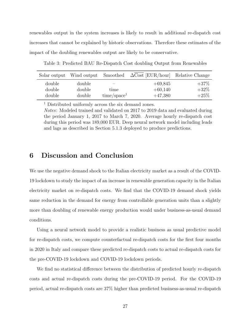
would affect re-dispatch costs without the lockdown demand reduction. We find that dou-

bling the output from renewable resources would increase re-dispatch costs by 37% during

the pre-lockdown period of January 1, 2017 to March 7, 2020. This result reinforces our con-

clusion that re-dispatch costs are likely to increase significantly as a result of an increasing

share of intermittent renewables at current demand levels.

Although the market response to an unexpected persistent net demand reduction caused

by the COVID-19 lockdown is likely to be different from a more gradual net demand reduction

caused by increased investments in wind and solar resources, our results demonstrate that

without investments in transmission expansions and other technologies for managing low

net demand as well as an effective local market power mitigation mechanism, the levels of

re-dispatch costs could rise rapidly. At these low net demand levels many system stability

constraints bind which can create new opportunities for suppliers providing these services to

increase the prices they are paid.

These results also underscore the need for regions with ambitious wind and solar energy

goals to adopt wholesale market designs that more closely match the economic model used

to set prices and generation output levels to the way the transmission network is actually

operated.10 Our results demonstrate that the opportunities for suppliers to profit from the

difference between the model used to operate the electricity market and how the grid is

actually operated scales rapidly as the average level of net demand falls.

The remainder of the paper is organized as follows. In Section 2, we describe the key fea-

tures of structure and operation of Italian electricity supply industry necessary to understand

our analysis. In Section 3, we show how the lockdown demand shock has affected market

outcomes in the Italian electricity market. In Section 4, we detail our approach to estimat-

ing the pre-COVID-19 relationship between system conditions and re-dispatch costs that

we subsequently use to predict counterfactual lockdown re-dispatch costs. In Section 5, we

10See Graf et al. (2020b) for an example of market participant behavior that can arise from a marketdesign that does not match the economic model used to set prices and output level to the way the system isactually operated.

5

present our results and investigate their robustness under alternative modeling assumptions.

We conclude the paper in Section 6.

2 The Operation of the Italian Wholesale Electricity

Market

The Italian wholesale electricity market consists of the European day-ahead market followed

by a series of domestic intra-day market sessions, and finally the real-time re-dispatch mar-

ket. The day-ahead market does not procure ancillary services, only energy. In the intra-day

market sessions, participants have the option to update the generation and demand sched-

ules that emerge from the day-ahead market or a previous intra-day market session. The

day-ahead market as well as all of the intra-day markets are zonal-pricing markets that ig-

nore transmission network constraints within the zone and other relevant generation unit

operating constraints in setting prices and generation unit output levels.11

Shortly after the day-ahead market clears, two out of the seven intra-day market sessions

are run, still one day in advance of actual system operation. After the clearing of the second

intra-day market, the first session of the re-dispatch market takes place. Five other re-

dispatch sessions will be run, one after each intra-day market session as well as a real-time

re-dispatch market session that clears every fifteen minutes.

In the real-time re-dispatch market, the objective is to balance any net demand forecast

errors but also to transform the schedules resulting from the zonal day-ahead and intra-

day market-clearing processes into final schedules that allow secure grid operation in real-

time by minimizing the combined as-offered and as-bid cost to change generation schedules.

Generation units that are needed to produce more output are paid as-offered to supply

this energy and generation units that are unable to produce as much energy because of

11Currently, the day-ahead market and intra-day markets consist of seven bidding zones (see Tables A.1and A.2 for more details).

6

a real-time operating constraint sell this energy as-bid. The solution to this optimization

problem accounts for a nodal network model, the possibility that equipment can fail, errors

in forecasts of demand or non-controllable generation, and ensures that technical parameters

such as frequency levels or voltage levels are within their security ranges. An offer to start-

up a unit or to change a unit’s configuration can be submitted to the real-time re-dispatch

market as well as price/quantity pairs to increase and decrease a units schedule. The re-

dispatch market is operated by the Italian transmission system operator (Terna). Between

2017 and 2019 the average annual real-time upward re-dispatch volume was 16 TWh and

downward re-dispatch volume was 19 TWh. More details on the market design can be found

in Graf et al. (2020a,b).

Graf et al. (2020b) find that market participants factor in the expected revenues they

can earn from being accepted in the re-dispatch market when they formulate their offers

into the day-ahead market. Suppliers recognize that the real-time operating levels of all

generation units must respect all network and generation unit-level operating constraints,

whether or not these constraints are accounted for in the day-ahead or the intra-day market-

clearing engine. Differences between the constraints on generation unit behavior that must

be respected in the day-ahead and intra-day markets and the additional constraints that

must be respected in the real-time operation of the transmission network are what create

the opportunities for suppliers to play what has come to be called the “INC/DEC Game.”

Ignoring the forecast error in locational net demand profiles between day-ahead and real-

time, demand for re-dispatch energy from a generation unit upward or downward arises if

a unit’s day-ahead market schedule is not compatible with secure operation of the grid in

real-time. The “INC/DEC Game” relies on the fact that the demand for re-dispatch from a

generation unit is endogenously determined by the owner’s day-ahead market offer and the

day-ahead market offers of other market participants. A high offer price in the day-ahead

market can cause a unit required to supply energy in real-time to fail to sell energy in the

day-ahead market. A low offer price in the day-ahead market can cause a unit that cannot

7

supply energy in real-time to sell energy in the day-ahead market.

This logic implies that a generation unit owner that is confident its unit is required to run

in real-time may offer this unit in the day-ahead market at extremely high price. The unit

would either be taken in the day-ahead market at this price or not taken in the day-ahead

market but subsequently taken in the re-dispatch market at this offer price or an even higher

offer price. The more confident the unit owner is that its unit will be needed to supply

energy in real-time regardless of its offer price in the re-dispatch market, the higher the offer

price the unit owner can submit into the day-ahead market.

Similar logic applies to the case of suppliers that are confident that their generation units

cannot supply energy in real-time because of a transmission network or other operating

constraint. In this case, the unit owner would submit a very low offer price into the day-

ahead market to ensure that it sells energy at the market-clearing zonal price. The more

confident the unit owner is that this energy cannot be supplied in real-time, the lower is the

offer price submitted into the day-ahead market. In the re-dispatch market this unit owner

will then buy back this energy at a bid price that is lower than the market-clearing zonal

price and earn the difference between the day-ahead zonal price and this bid price times the

amount of energy it is unable to supply.

In regions that employ zonal day-ahead and intra-day markets and operate a pay-as

offered and buy as-bid re-dispatch process, the opportunities for controllable generation units

to profit from the predictability of net demand conditions that make their units necessary to

operate or not operate are likely to increase as the amount intermittent renewable generation

increases.12 In Table 1, Panel A, we detail the actual installed capacity of wind and solar

between 2012 and 2020 in the Italian market. Installed capacities of solar has been steadily

increasing from 17 GW to 21 GW and of wind from 8 GW to 11 GW. In Panel B, we show

several projections for the years 2025, 2030, and 2040. Notably, solar capacity is projected

to more than double in two out of three scenarios for 2030. Wind capacity is also projected

12Investments in resources that provide flexibility, such as storage, demand response, and transmissionnetwork upgrades can reduce the frequency that these opportunities arise.

8

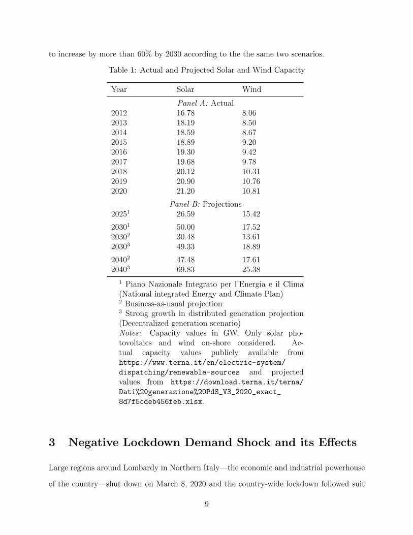
to increase by more than 60% by 2030 according to the the same two scenarios.

Table 1: Actual and Projected Solar and Wind Capacity

Year Solar Wind

Panel A: Actual2012 16.78 8.062013 18.19 8.502014 18.59 8.672015 18.89 9.202016 19.30 9.422017 19.68 9.782018 20.12 10.312019 20.90 10.762020 21.20 10.81

Panel B: Projections20251 26.59 15.42

20301 50.00 17.5220302 30.48 13.6120303 49.33 18.89

20402 47.48 17.6120403 69.83 25.38

1 Piano Nazionale Integrato per l’Energia e il Clima(National integrated Energy and Climate Plan)2 Business-as-usual projection3 Strong growth in distributed generation projection(Decentralized generation scenario)Notes : Capacity values in GW. Only solar pho-tovoltaics and wind on-shore considered. Ac-tual capacity values publicly available fromhttps://www.terna.it/en/electric-system/

dispatching/renewable-sources and projectedvalues from https://download.terna.it/terna/

Dati%20generazione%20PdS_V3_2020_exact_

8d7f5cdeb456feb.xlsx.

3 Negative Lockdown Demand Shock and its Effects

Large regions around Lombardy in Northern Italy—the economic and industrial powerhouse

of the country—shut down on March 8, 2020 and the country-wide lockdown followed suit

9

on March 10, 2020. In the days that followed, the lockdown became even more stringent by

narrowing the definition of what an essential business is. The strict lockdown was eased on

April 26, 2020.

In Figure 2, we show how the lockdown of effectively all non-essential businesses in a

response to the COVID-19 outbreak drastically reduced the national demand for electricity.

In Panel (a), we compare the BAU average weekly demand profile, that we define as the

hourly average demand in March and April during the years 2017 through 2019 for each hour

of the week, to the demand profile during the seven weeks of lockdown (March 9, 2020 until

April 26, 2020),13 where the first hour of the week is the hour beginning Monday at 00:00

AM. The figure demonstrates that the average hourly demand is lower in all hours of the

week during the lockdown period. In Panel (b), we show how the daily average of demand

has changed relative to the daily average demand for each day-of-week between January and

April over the years 2017 through 2019. Average daily demand for the lockdown period is

20% less than the average daily demand during same time period in 2017 through 2019.

An increasing number of electricity markets have a considerable share of non-controllable

supply. Non-controllable supply includes generation from renewables, such as wind, solar,

or hydro. In Europe, net-imports made through either long-term allocation processes or

the joint European day-ahead market-clearing are non-controllable in real time except for

emergency situations. Higher net imports and more output from non-controllable units will

reduce the demand that will be served by controllable generation units, including fossil-fuel

generators but also storage units.

We define the hourly net demand (ND) for controllable generation units for each bidding

zone z as follows

NDz = Dz −RESz −Hydroz − Impz, (1)

13We define the lockdown period throughout the paper to range between Sunday, March 8, 2020 andSunday, April 26, 2020. However, for the graphs showing weekly averages, we decided to skip hourlyobservations from Sunday, March 8, 2020, to obtain the same number of observations for each week.

10

whereas D is system demand, RES the supply from intermittent renewable sources such as

wind or solar, Hydro is non-dispatchable hydro production, such as generation from run-

of-river plants, and Imp is net imports from foreign countries. We use the same logic to

create day-ahead net demand forecast (NDFC) variables by replacing D and RES with their

day-ahead forecasts. Note that non-controllable hydro schedules as well as net imports from

foreign countries are firm after the day-ahead market-clearing.

Figure D.2 shows hourly net demand boxplots for the BAU period and the lockdown

periods. BAU period net demands are from hours in March to April for the years 2017

through 2019. Lockdown net demands are for hours between 2020-03-08 and 2020-04-26.

Boxes represent the interquartile range (IQR) and the upper and lower vertical bars are the

1 percentile and 99 percentile for that hour of the day. Diamonds represent outliers not

included in the 1 to 99 percentile range. The average hourly lockdown period net demand

was 21% lower than the BAU period average hourly net demand.

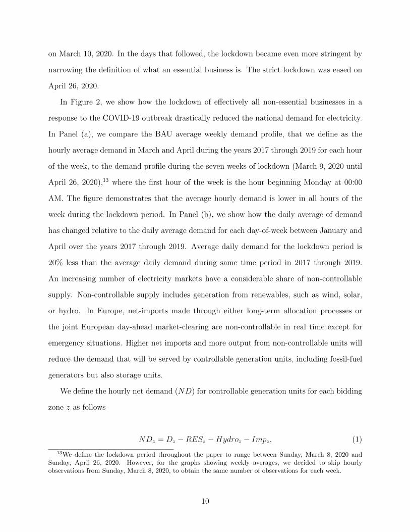
Panel (a) of Figure 3 plots the net demand duration curve for the years 2017 through

2019. Panel (b) plots the net demand duration curve for the lockdown period from 2020-03-

08 to 2020-04-26. Although the range of net demands from 2017 to 2019 is larger than the

range of net demands during the lockdown period, the range of net demand from 2017 to

2019 contains the range of net demands during the lockdown period. The shape of the net

demand duration curve in panel (a) is similar to the shape of the net demand duration curve

in panel (b). The major difference between the two curves is that much more probability

mass is concentrated in a much smaller range of low demand levels during the lockdown

period.

In Figure 1, Panel (a), we show how the negative demand shock affected day-ahead

electricity prices compared to BAU. As expected, a negative demand shock paired with lower

input prices to produce electricity led to lower electricity prices. Average lockdown period

hourly day-ahead market prices were down by 45% compared to average BAU period hourly

day-ahead market prices. Although these lower day-ahead market prices are good news for

11

the final consumer, in simplified European electricity market designs where system security

constraints are only accounted for in the real-time re-dispatch market, the final consumer

also pays the cost of re-dispatching generation units to achieve physically feasible generation

output levels to meet real-time demand at all locations in the transmission network.

In Figure 1, Panel (b), we show average hourly re-dispatch costs per MWh of demand

during lockdown and BAU period applying the same definition for BAU as above.14 We find

that average hourly re-dispatch costs per MWh of demand increased by 108% during the

lockdown compared to the BAU period. For some weeks during the lockdown, the average

re-dispatch cost per MWh of demand was almost as high as the day-ahead market price.

The sharp increase in the re-dispatch costs drastically reduces the electricity cost savings for

the final consumers due to the reduced electricity demand during the lockdown.

4 Estimating BAU Period Re-Dispatch Cost

In this section, we estimate a model that predicts the BAU period re-dispatch costs using

data on system conditions. This model is then used to predict re-dispatch costs during

the lockdown period. Because this model is estimated using data from 2017–2019, the

lockdown period predictions from this model cannot capture changes in offer behavior or

system security requirements caused by the persistent low net demand levels that occurred

during the lockdown period. This model can only use relationship between system conditions

and re-dispatch costs during weekends and holidays during the BAU period to predict re-

dispatch coss for comparable low net demand periods during the lockdown period.15

The main factors used to predict re-dispatch costs are the zonal net demands—the de-

mand within each zone that must to be served by controllable generation units. We also

14Hourly real-time re-dispatch costs are computed as the sum of the awarded incremental real-time re-dispatch quantities valued at the as-offered costs net of the sum of the awarded decremental real-timere-dispatch quantities valued at the as as-bid costs. As-offered costs to start-up a unit or to change a unit’sconfiguration are neglected.

15In fact, the lowest level of net demand found in our sample was observed in a pre-covid hour, i.e., on aSunday afternoon in June (2019-06-02, 2 pm to 3pm).

12

Figure 1: Electricity Prices versus Re-dispatch Costs

(a) (b)

Notes: Panel (a): Business-as-usual (BAU) day-ahead market electricity price calculated as the averageprice for each hour of the week over March and April in the years 2017–2019. Lockdown electricity pricecalculated as the average price between March 9, 2020 and April 26, 2020. Panel (b): BAU re-dispatchcosts calculated as the average costs per MWh of demand for each hour of the week over March and Aprilduring the years 2017–2019. Lockdown re-dispatch costs calculated as the average hourly costs per MWhof demand between March 9, 2020 and April 26, 2020. Shaded area around the mean values represents thepointwise 95% confidence interval. Data sources to derive the graph described in Table A.1.

include the day-ahead forecast of zonal net demands. It is important to include actual and

forecast zonal net demands because the re-dispatch quantities for each generation unit is the

difference between its real-time output and its day-ahead market schedule. For example if

demand was underestimated day-ahead, the demand for re-dispatch will be higher because of

the forecast error while it will be lower or even negative for an overestimation of day-ahead

demand. However, the uncertain forecast error is not the only reason for a (locational)

demand for re-dispatch. System operation constraints such as voltage regulation, reserve

requirements or nodal network constraints also drive the demand for re-dispatch actions.

We include zonal net demand levels because the spatial distribution of net demand reveals

(i) inter-zonal power flows16 and (ii) are useful predictors for whether system constraints

16Across-zone power flows are implicitly defined by zonal balances in a radial network and the currentItalian network configuration supports this assumption to a large extent. The zonal net demands result in so-called base-flows and the market power that includes the power to congest a network by market participantswith controllable units in their portfolio will affect the final flows through their offer behavior (see, e.g., Graf

13

Figure 2: Demand-Shock Due to Lockdown in Response to COVID-19 Pandemic

(a) (b)

Notes: Panel (a): Business-as-usual (BAU) demand (market load) calculated as the average demand for eachhour of the week over March and April in the years 2017–2019. Lockdown demand calculated as the averagedemand between March 9, 2020 and April 26, 2020. The first hour of the week starts on Monday 00:00 AM.Panel (b): Daily demand change relative to daily baseline demand, that is, the daily average demand foreach day-of-week between January and April over the years 2017–2019. Dotted vertical line indicates thedate of when the lockdown began (March 8, 2020). Data sources to derive the graph described in Table A.1.

will bind. We also include the day-ahead market price to control for the variable cost of

the marginal generation unit. We include a workday indicator variable that is equal to one

for days that are not weekend days nor holidays. Finally, we include an indicator for the

months December to April because the thermal capacity of overhead transmission lines is

higher during these months because of lower ambient temperatures levels. Note that our

goal is to predict hourly BAU re-dispatch costs for the current day given current system

conditions and not to predict re-dispatch costs for a day in the future. Therefore, we believe

it is legitimate to use data from the previous day and current day for this purpose.

We compiled data on the variables described above for the time period 2017-01-01 to

2020-04-26. A more detailed description of the variables and their sources can be found in

Table A.1. Descriptive statistics of relevant variables are presented in Table A.2.

Instead of using regression based models, we use a deep neural network model with

and Wolak, 2020, for more details on unilateral market power that includes congestion power in locationalmarkets).

14

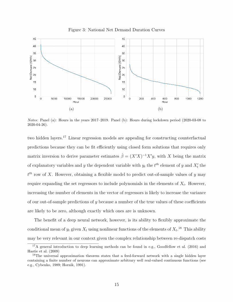
Figure 3: National Net Demand Duration Curves

(a) (b)

Notes: Panel (a): Hours in the years 2017–2019. Panel (b): Hours during lockdown period (2020-03-08 to2020-04-26).

two hidden layers.17 Linear regression models are appealing for constructing counterfactual

predictions because they can be fit efficiently using closed form solutions that requires only

matrix inversion to derive parameter estimates β = (X ′X)−1X ′y, with X being the matrix

of explanatory variables and y the dependent variable with yt the tth element of y and X ′t the

tth row of X. However, obtaining a flexible model to predict out-of-sample values of y may

require expanding the set regressors to include polynomials in the elements of Xt. However,

increasing the number of elements in the vector of regressors is likely to increase the variance

of our out-of-sample predictions of y because a number of the true values of these coefficients

are likely to be zero, although exactly which ones are is unknown.

The benefit of a deep neural network, however, is its ability to flexibly approximate the

conditional mean of yt given Xt using nonlinear functions of the elements of Xt.18 This ability

may be very relevant in our context given the complex relationship between re-dispatch costs

17A general introduction to deep learning methods can be found in e.g., Goodfellow et al. (2016) andHastie et al. (2009)

18The universal approximation theorem states that a feed-forward network with a single hidden layercontaining a finite number of neurons can approximate arbitrary well real-valued continuous functions (seee.g., Cybenko, 1989; Hornik, 1991).

15

and input variables. Consequently, if the researcher is willing to tolerate some bias in the

estimation of the conditional expectation of yt given Xt, an out-of-sample prediction of

ys given Xs that has smaller expected mean-squared error prediction is possible. A deep

neural network assumes E(yt|Xt) = f(Xt; β). The parameter vector β—called weights in the

machine learning jargon—of this nonlinear function are chosen to minimize the in-sample

mean-squared prediction error as well as accounting for the possibility of within-sample over-

fitting. In a two hidden layer neural network three functions are connected in a chain to form

f(x) = f (3)(f (2)(f (1)(x))), with f (1) being the first hidden layer, f (2) the second hidden layer,

and f (3) being the last layer, called the output layer. The learning algorithm’s objective is to

optimally use the layers to best approximate E(yt|Xt). We refer to Chapter 6 in Goodfellow et

al. (2016), or Chapter 11 in Hastie et al. (2009) for more details. The cost of this deep neural

network approach is that many model parameters have to be estimated in an iterative process

using numerical optimization methods, often with objective function penalties on certain

tuning parameters. We detail the model’s configuration and our strategies to circumvent

known potential shortcomings such as model uncertainty or over-fitting in Appendix C.

A major concern of all machine learning models is over-fitting. We address this issue by

using the method of cross-validation for model selection. The basic idea of this method is to

split the in-sample data ranging from January 1, 2017 to December 31, 2019 into a training

sample and a validation sample. The parameters are estimated on the training sample

and the validation sample is used to monitor out-of-training-sample performance (the mean

squared error, i.e., the average squared difference between the estimated re-dispatch cost and

the actual re-dispatch cost) and set the values of various tuning parameters in estimation

samples. The performance on the validation set is used as a proxy for the generalization

error and model selection is carried out using this measure see discussed in Rasmussen and

Williams (2006). We use a random 70:30 split, i.e., 70% of the data will be used for training

the model and 30% for validating the model. This approach will make the trained weights

(parameter estimates) more generally applicable rather than being too strongly tailored to

16

the estimation or training data. We also set aside a considerable part of the overall data

that is not presented to the algorithm for training or for validation (see Appendix B for more

details). We divide this out-of-sample data into “pre-lockdown”-data ranging from January

1, 2020 to March 7, 2020 and “lockdown”-data ranging from March 8, 2020 to April 26, 2020

(see Figure B.1 for a graphical summary of the design).

5 Results

In Figure 4, we present the out-of-sample prediction error for the pre-lockdown period (2020-

01-01 to 2020-03-07) and the lockdown period (2020-03-08 to 2020-04-26). The prediction

error is defined as the difference between predicted BAU re-dispatch cost from our neural

network model and actual re-dispatch cost. Hence a negative prediction error means that

we have underestimated the actual re-dispatch cost. The average hourly prediction error

during the BAU period is about −2, 000 EUR (a 1% percentage error relative to the average

predicted BAU re-dispatch cost) while the average prediction error during lockdown period is

orders of magnitude larger at −107, 000 EUR (a 37% percentage error relative to the average

predicted BAU re-dispatch cost. Furthermore, the prediction error distribution during the

lockdown period is more negatively skewed than the prediction error distribution during the

BAU period. A Wilcoxon Signed Rank test comparing the distributions of predicted versus

actual re-dispatch costs for the BAU period finds that these distributions are not statistically

different at the 5% level (p-value: 0.23).19 Applying the same test to the lockdown period

yields a p-value that is effectively zero, indicating that the distribution of predicted re-

dispatch costs during the lockdown period is statistically significantly different from the

distribution of actual re-dispatch costs during this same time period.

In Figure 5, Panel (a), we compare the daily re-dispatch costs to our predicted BAU

re-dispatch costs. We add a prediction error band around our point estimates to account for

19To derive the p-value an asymptotic normal approximation to the null distribution of the test statisticis used.

17

the uncertainty in the predictions. More precisely, we add the absolute value of the 0.025

quantile of the prediction error during the out-of-sample pre-lockdown period to the point

estimates of the lockdown period and subtract the 0.975 quantile from the point estimates.

The figure in Panel (a) shows that before the lockdown our model estimates are well within

the prediction bands, whereas that is not the case during the lockdown period. In Panel

(b), we zoom into the lockdown period and compare hourly values of the actual re-dispatch

costs and our predicted BAU re-dispatch costs, showing that realizations in some hours are

substantially larger than our predictions.

Overall, we find that the actual average hourly re-dispatch costs during the lockdown were

37% higher than our BAU estimates during the lockdown and our BAU estimates during

the lockdown are 26% higher than the average hourly re-dispatch costs during the same

time period in previous years. As noted earlier, the average hourly re-dispatch cost during

the lockdown is 73% higher than the average hourly re-dispatch costs during the same time

period in previous years. Therefore, roughly two-thirds of the increase in re-dispatch costs

during the lockdown can be attributed to the persistent low net demand conditions giving

market participants more opportunities to figure out schedule configurations that increase

the demand for re-dispatch actions. Furthermore, a higher demand for storage units is

created20 and amplified the impact of market power exercise, that cannot be explained by

the past relationship between system conditions and re-dispatch costs.21

The 37% increase in actual re-dispatch cost compared to our BAU predictions during the

lockdown amounts to 129 million EUR for the seven weeks of strict lockdown. In a world

20Low net demand hours may require to dispatch storage units to increase net demand for accommodatingsystem-relevant thermal generation units. The reservoir balance constraints of storage units make it necessaryto also release the stored electricity (in form of water) within a short period of time to have spare head-roomin the reservoirs to increase net demand again in the near future if necessary. Therefore, part of the availablestorage capacity may have considerable market power in settings with persistently low net demand becausethey face little competition in the market for increasing net-demand in real-time.

21Although average re-dispatch costs on non-business days before the lockdown are comparable to thoseon workdays during the lockdown, average hourly re-dispatch costs were 308,000 EUR for non-business daysbefore the lockdown and 332,000 EUR only on workdays during the lockdown. This yields a 8% increasedespite lower fuel costs during the lockdown period. The average hourly re-dispatch cost during lockdownusing all hours yields 395,000 EUR. Hence, an increase of over 25% compared to non-business days in Marchand April over the years 2017–2019.

18

with a large share of renewables, the reduced net demand situation would be permanent.

Hence, to put things into perspective and extrapolating this amount to an annual level

yields an increase in the re-dispatch cost by almost 1 billion EUR per year. As noted earlier,

the negative COVID-19 demand led to a net demand reduction that is the equivalent of

doubling renewable energy production in Italy. Consequently, using these numbers implies

the potential for a roughly 1 billion EUR increase re-dispatch costs associated with a roughly

doubling of renewable energy production in Italy under the existing market design.

Figure 4: Distribution Out-of-Sample Prediction Errors

Notes: The prediction error is defined as the difference between the predicted out-of-sample pre-lockdownre-dispatch costs and the actual re-dispatch costs realizations. Out-of-sample pre-lockdown period rangesfrom January 1, 2020 to March 7, 2020 and out-of-sample lockdown period from March 8, 2020 to April 26,2020.

19

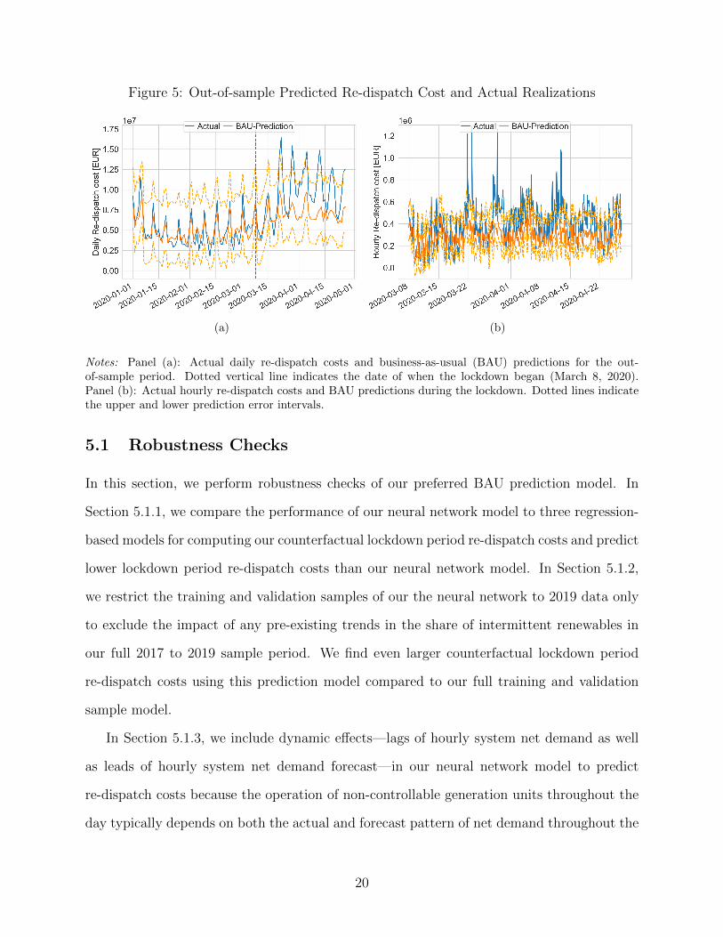
Figure 5: Out-of-sample Predicted Re-dispatch Cost and Actual Realizations

(a) (b)

Notes: Panel (a): Actual daily re-dispatch costs and business-as-usual (BAU) predictions for the out-of-sample period. Dotted vertical line indicates the date of when the lockdown began (March 8, 2020).Panel (b): Actual hourly re-dispatch costs and BAU predictions during the lockdown. Dotted lines indicatethe upper and lower prediction error intervals.

5.1 Robustness Checks

In this section, we perform robustness checks of our preferred BAU prediction model. In

Section 5.1.1, we compare the performance of our neural network model to three regression-

based models for computing our counterfactual lockdown period re-dispatch costs and predict

lower lockdown period re-dispatch costs than our neural network model. In Section 5.1.2,

we restrict the training and validation samples of our the neural network to 2019 data only

to exclude the impact of any pre-existing trends in the share of intermittent renewables in

our full 2017 to 2019 sample period. We find even larger counterfactual lockdown period

re-dispatch costs using this prediction model compared to our full training and validation

sample model.

In Section 5.1.3, we include dynamic effects—lags of hourly system net demand as well

as leads of hourly system net demand forecast—in our neural network model to predict

re-dispatch costs because the operation of non-controllable generation units throughout the

day typically depends on both the actual and forecast pattern of net demand throughout the

20

day. These models predict higher counterfactual lockdown period re-dispatch costs than our

preferred model, but the difference between the distribution of predicted re-dispatch costs

during the lockdown period from this model and the actual distribution of re-dispatch costs

during the lockdown period are still statistically different. In Section 5.1.4, we use a neural

network model estimated over our 2017 to 2019 period to predict the impact of doubling

of actual renewable output during 2017-01-01 to 2020-03-07. We find that predicted re-

dispatch costs during this time period are roughly 37% above actual re-dispatch costs during

this time period. This predicted increase in re-dispatch costs (due a doubling of renewable

output) relative to actual re-dispatch costs during the pre-lockdown period is larger than

the predicted increase in re-dispatch costs during the lockdown compared to BAU period re-

dispatch costs, i.e., average hourly re-dispatch costs during the same time period in previous

years.

5.1.1 Regression-based Models

In Table 2, Panel A, we present the pre-lockdown out-of-sample performance of several

regression-based models estimated over our 2017 to 2019 training and validation sample pe-

riod. Unlike in the deep-learning framework, we run the linear regressions on the combined

training and validation samples. We use the root mean square error (RMSE) metric22 evalu-

ated at pre-lockdown out-of sample observations and predictions to compare the performance

of all our models. Our preferred deep neural network specification described in Section 5

yields an RMSE of 81,676 EUR for the period 2020-01-01 to 2020-03-07 (the actual average

hourly re-dispatch cost for the same period yields 206,000 EUR) . Using the same set of

explanatory variables X =

[XC XI

]with XC containing the continuous variables (day-

ahead market price, zonal net demands, and zonal day-ahead net demand forecasts), and XI

the indicator variables (workday indicator variable and winter indicator variable), as input

in estimating a linear model by ordinary least squares yields an RMSE of 103,120 EUR.

22RMSE(y, y) =√T−1

∑Tt=1(yt − yt)2.

21

As discussed in Section 4, the advantage of the deep-learning framework is that it spec-

ifies a flexible nonlinear function for E(yt|Xt). A popular approach to account for more

flexible functional forms in regression based model is to include polynomial terms and in-

teraction terms. We therefore include 2nd degree polynomials and interaction terms of the

continuous explanatory variables. This modification of the regression model pushes the

pre-lockdown out-of-sample RMSE down to 85,904 EUR—a drastic improvement that is

nonetheless slightly higher than the goodness of fit of our deep neural network model. A

tempting strategy to reduce the pre-lockdown RMSE would be to add higher degree polyno-

mials and interaction terms. However, adding 3rd degree polynomials and interaction terms

of the columns of XC to the regression model actually drastically increases the pre-lockdown

out-of-sample RMSE to 104,505 EUR. This is a typical of out-of-sample prediction behavior

of an over-fitted linear regression model which can be mitigated by the use of our preferred

neural network approach.

All three regression models summarized in Table 2 yield lower total predicted BAU re-

dispatch costs during the lockdown than our neural network model. Therefore the actual

average re-dispatch costs relative to the average predicted BAU re-dispatch costs during the

lockdown are larger (+55% to +80% compared to +37% of our preferred deep neural network

model). In that sense, our preferred deep neural network model leads to a more conservative

conclusion on the additional re-dispatch cost increase during the lockdown compared to the

regression based model predictions.

5.1.2 Trend in In-sample Data

On an annual basis we find that re-dispatch costs have increased in 2019 to 1.83 billion EUR

compared to 1.53 billion in 2017 and 1.57 billion in 2018. A potential explanation could be

that the output from wind was higher in 2019; 19.9 TWh compared to 17.5 TWh in 2017

and 17.3 TWh in 2018. Wind capacity is mainly concentrated in the South of the country

where the transmission network is less extensive, which may explain this difference. To check

22

whether this trend in renewable output over our 2017 to 2019 training and validation sample

period could explain the level of our predicted re-dispatch cost increase during the lockdown

period, we train our model using only data from 2019. More precisely, we adapt the same

cross-validation strategy to circumvent over-fitting as before with the only difference that we

perform the random sample split on observations that occurred in the year 2019. All other

choices of how we implemented our preferred specification of the neural network including

hyper-parameter optimization are unchanged and so are the input variables. Instead of a

37% additional increase in the actual lockdown re-dispatch costs relative to the predicted

re-dispatch costs, we find a 43% increase when training our prediction model on this reduced

sample.

5.1.3 Dynamic Effects

Although, the day-ahead market is cleared hour by hour, market participants’ offer strategies

that determine the schedules of their conventional dispatchable units are likely to condition

on the recent past and forecasts of near future states of the system because of non-convexities

in the units’ production functions.23 Hence, we add 24 hours of lagged system net demand

variables to the set of explanatory variables.24 This modeling choice slightly decreases the

RMSE from 81,676 EUR to 80,863 EUR as presented in Table 2, Panel B. Adding 24 hour

of leads of the system net demand forecast25 slightly decreases the pre-lockdown out-of

sample RMSE to 80,363 EUR. If we were to choose a model based on pre-lockdown out-of-

sample performance, we would select the model with the 24 lagged hourly variables and 24

lead hourly variables. This model also yields a larger average predicted BAU re-dispatch

costs during the lockdown. Therefore the actual average re-dispatch costs relative to the

23They non-convexities include start-up and minimimum operating level costs and minimum up-time,minimum down-time, and ramping constraints.

24The regressor matrix in this specification is defined as X =

[XC XI

{Lk (

∑z NDz)

}k∈{1,...,24}

],

with L being the lag operator.25The regressor matrix in this specification is defined as X =[

XC XI{

Lk (∑

z NDz)}k∈{1,...,24}

{L−k

(∑z NDFC

z

)}k∈{1,...,24}

].

23

average predicted BAU re-dispatch costs during the lockdown are lower (+11% compared to

+37%). The prediction errors of both dynamic model specifications imply Wilcoxon signed

rank statistics indicating statistically significantly different distributions of predicted BAU

versus actual re-dispatch costs. Hence, the qualitative interpretation of our results remain

unchanged for these dynamic models to predict re-dispatch costs.

Table 2: Model Comparison based on Pre-Lockdown Out-of-sample Performance

Polynomials/Interactions1 Lags2 Leads3 RMSE4 Actual costPredicted BAU cost

5

Panel A: Linear regression model– – – 103,120 +82%

2nd degree – – 85,904 +55%2nd and 3rd degree – – 104,505 +80%

Panel B : Deep neural network– – – 81,676 +37%– 24 hours – 80,863 +17%– 24 hours 24 hours 80,363 +11%

1 nth degree polynomials and interaction terms of continuous explanatoryvariables, i.e., zonal net demands, zonal net demand forecasts, and day-ahead market price.2 Lags of system net demand.3 Leads of system net demand forecast.4 RMSE(y, y) =

√T−1

∑Tt=1(yt − yt)2.

5 Average actual hourly re-dispatch costs during lockdown relative to pre-dicted BAU re-dispatch costs.

5.1.4 Renewables and the Cost to Re-dispatch

One concern with our preferred results is that our predicted re-dispatch cost increase during

the lockdown may be a lower bound on re-dispatch cost increase associated with the equiva-

lent decrease in net demand from a larger share of intermittent renewables. That is because

the lockdown demand shock may have been more evenly distributed (over time and space)

than it would be the case if the share of intermittent renewables increased substantially. We

are not able to test this hypothesis directly because the lockdown re-dispatch cost observa-

tions resulted from a negative demand shock. However, we can analyze how the effect of an

24

increased share of solar and wind output would change the cost to re-dispatch the system

using our BAU prediction model.26 More precisely, we conduct three counterfactuals with

different assumptions on how the increased output of renewables will be distributed over

time and space. The overall reduction of zonal net demands is the same under all three

scenarios.

We use the dynamic model presented in Section 5.1.3 with the only exception that we

replace the day-ahead market price by the daily natural gas price to account changes in the

input fuel costs. There exists an ample literature on how more output from low variable cost

renewables will depress day-ahead market prices (see e.g., Sensfuß et al., 2008; Wurzburg

et al., 2013; Clo et al., 2015; Sanchez de la Nieta and Contreras, 2020) and on how more

output from renewables will affect the intra-day variance in hourly day-ahead market prices

(see e.g., Wozabal et al., 2016). Hence, when manipulating the output from renewables

we cannot treat the day-ahead market price as exogenous variable any longer and therefore

replace it by the daily gas price assuming that this price is unaffected by a modified aggregate

renewables output profile. We believe that applying a dynamic model is important in this

particular setting because especially solar with its unimodal output distribution will likely

change the operation of many conventional units.

The first counter-factual analysis involves scaling the existing locational (zonal) output

from wind and solar by factor two.27 The simplifying assumptions behind this scaling ap-

proach is that the frequency of binding intra-zonal transmission constraints will not increase.

Furthermore, we assume that weather patterns within a zone are comparable and that the

zonal distribution of additional renewable generation capacity will be equal to the current

26We refer to Gianfreda et al. (2018) for a graphical analysis detailing how the increase in capacity fromrenewables may have increased the real-time re-dispatch cost in Italy’s northern bidding zone comparing theyears 2006–2008 (almost no renewable capacity) to the years 2013–2015. Gianfreda et al. (2016) calculateprice premia between the Italian day-ahead (intra-day) market prices and awarded quantity-weighted averagereal-time re-dispatch market payments and find that renewables generally increase those. Bigerna et al.(2016) analyzes zonal Lerner indices during the period 2009 to 2013 for the main generators in the Italian day-ahead market and conclude that the exercise of market power in the day-ahead market has been surprisinglyreinforced in specific off-peak hours as a result from increased supply from renewables.

27Table 1, Panel B, shows several projections on the growth of wind and solar capacity in Italy and findthat wind and solar capacity may already be doubled in the next decade from now.

25

distribution. All other factors that define the zonal net demands and day-ahead forecasts

are unchanged.

We use our deep neural network model trained and validated on 2017 to 2019 data to

predict the hourly re-dispatch costs between 2017-01-01 and 2020-03-07 for the net demand

implied by our counterfactual renewable output. Table 3 shows that doubling the output

from solar and wind generation units leads to an increase in the predicted re-dispatch cost

by 37% (Table 3, first row). This percent increase is larger than the percent increase that

predicted lockdown re-dispatch costs are relative to our counterfactual BAU lockdown period

re-dispatch costs from past years (26%). One reason for this deviation may be that the larger

sample length is more informative and portrays a better overall picture. Another potential

explanation is that the variable output from renewables has greater impact on re-dispatch

costs than a persistent demand shock—a hypothesis we investigate in the next paragraphs.

The second counter-factual analysis aims to quantify the effect of intermittency and

temporal variation in the output of renewables. We therefore reduce the zonal net demands

and net demand forecasts uniformly by the sample average output of wind and solar units

in each zone.28 This exercise yields a predicted increase in the re-dispatch costs of 32%

(Table 3, second row) during period 2017-01-01 and 2020-03-07.

Lastly, we modify the spatial distribution smoothing the additional renewables along

time and space.29 This exercise yields a predicted increase in the hourly re-dispatch cost by

only 25% (Table 3, third row) for the period 2017-01-01 to 2020-03-07.

These findings emphasize the importance of the various seasonalities of renewable tech-

nologies, the importance of their location, as well as the associated forecast errors between

day-ahead prediction and real-time output of renewables. These final two estimates em-

phasize that increased spatial and temporal variation in renewables output as the share of

28We calculate the average actual output of solar and wind for each zone and net this value from eachzone’s net demand.

29We distributed the additional output from renewables uniformly across the six demand zones. Putdifferently, we calculate the average aggregate output of solar and wind units and net one sixth of this valuefrom the zonal net demands.

26

renewables output in the system increases is likely to result in additional re-dispatch cost

increases that cannot be explained by historic observations. Therefore these estimates of the

impact of the doubling renewables output are likely to be conservative.

Table 3: Predicted BAU Re-Dispatch Cost doubling Output from Renewables

Solar output Wind output Smoothed ∆Cost [EUR/hour] Relative Change

double double – +69,845 +37%double double time +60,140 +32%double double time/space1 +47,380 +25%

1 Distributed uniformly across the six demand zones.Notes : Modeled trained and validated on 2017 to 2019 data and evaluated duringthe period January 1, 2017 to March 7, 2020. Average hourly re-dispatch costduring this period was 189,000 EUR. Deep neural network model including leadsand lags as described in Section 5.1.3 deployed to produce predictions.

6 Discussion and Conclusion

We use the negative demand shock to the Italian electricity market as a result of the COVID-

19 lockdown to study the impact of an increase in renewable generation capacity in the Italian

electricity market on re-dispatch costs. We find that the COVID-19 demand shock yields

same reduction in the demand for energy from controllable generation units than a slightly

more than doubling of renewable energy production would under business-as-usual demand

conditions.

Using a neural network model to provide a realistic business as usual predictive model

for re-dispatch costs, we compute counterfactual re-dispatch costs for the first four months

in 2020 in Italy and compare these predicted re-dispatch costs to actual re-dispatch costs for

the pre-COVID-19 lockdown and COVID-19 lockdown periods.

We find no statistical difference between the distribution of predicted hourly re-dispatch

costs and actual re-dispatch costs during the pre-COVID-19 period. For the COVID-19

period, actual re-dispatch costs are 37% higher than predicted business-as-usual re-dispatch

27

costs. Blowing up this increase in re-dispatch costs during the COVID-19 period to an annual

value and using the fact that the demand reduction implies a doubling of renewable energy

production implies a roughly 1 billion EUR annual increase in re-dispatch costs associated

with doubling renewable output. We emphasize that this re-dispatch cost increase is not a

prediction of how these costs will scale with an increased wind and solar generation share.

They are only indicative of how much these costs could increase without system operators

making the necessary investments in transmission and other technologies to manage the

lower levels of net demand that result from an increased share of intermittent renewables.

There are several reasons why a substantial increase in the share of renewables may

have an even more severe effect on re-dispatch costs in the Italian market than a negative

demand shock. First, there is a difference in expected shape and location to net demand

from a reduction in gross demand versus an increase in intermittent renewables. In the

case of solar, an energy-equivalent increase would have a far more concentrated diurnal

(and seasonal) shape than an energy-equivalent decrease in gross demand, occurring across

all hours. For wind, the diurnal shape may not be as concentrated, but the location is. In

both of these situations—the more concentrated shape and concentrated location—one could

reasonably expect higher re-dispatch costs from the increase in renewables, as compared to

the decrease in gross demand. Second, going beyond hourly averages to hourly variances,

there is likely to be a big difference in the volatility of hourly net demand from an increase

in renewables versus a decrease in gross demand due to the former’s intermittency. We have

shown that both effects are present in our analyses of different counterfactual renewable

output increases in Section 5.1. However, as we learned from our lockdown period analysis

in Section 5 an additional re-dispatch cost increase is likely as result of persistently lower

net demands, so our estimate of the increase of re-dispatch costs is on the conservative side.

We should also note that our analysis points out the need for market power mitigation

mechanisms to deal with a new source of local market power—that due low levels of net

demand. Traditional market power mitigation mechanisms focus on high demand hours as

28

these were the hours were little supply capacity will be left to compete with each other to

serve demand. According to this logic, low demand hours are not typically thought to be

periods when suppliers can exercise unilateral market power because there is plenty of idle

generation capacity. However, commitment costs, system security constraints, or transmis-

sion constraints are the reasons for market power potential in low demand hours. Although

grid upgrades can help in relieving these system security constraints and, consequently, the

opportunities to exercise local market power, these investments can have long lead-times

(ranging from few years, in the case of devices located inside substations, to decades, in the

case of transmission lines) and in a dynamic environment it is hard to anticipate what will

be needed in years to decades from now. Therefore, dynamic on-line market power mitiga-

tion systems could be useful to mitigate high re-dispatch costs as seen during the lockdown.

Such systems have the capacity to properly mitigate local market power even when the power

system is affected by unexpected events.

References

Benatia, David, Clemence Alasseur, and Olivier Feron, “Ring the Alarm! Electricitymarkets, Renewables, and the Pandemic,” USAEE Working Paper 20-473 2020.

Bigerna, Simona, Carlo Andrea Bollino, and Paolo Polinori, “Renewable Energyand Market Power in the Italian Electricity Market,” The Energy Journal, 2016, 37 (SI),123–144.

Borenstein, Severin, “Petro Questions and (Some) Answers,” Energy Institute BlogMay 18, 2020, UC Berkeley 2020. https://energyathaas.wordpress.com/2020/05/18/petro-questions-and-some-answers.

Clo, Stefano, Alessandra Cataldi, and Pietro Zoppoli, “The merit-order effect in theItalian power market: The impact of solar and wind generation on national wholesaleelectricity prices,” Energy Policy, 2015, 77, 79–88.

Cybenko, George, “Approximation by Superpositions of a Sigmoidal Function,” Mathe-matics of Control, Signals, and Systems, 1989, 2, 303–314.

Gianfreda, Angelica, Lucia Parisio, and Matteo Pelagatti, “The Impact of RES inthe Italian Day-Ahead and Balancing Markets,” The Energy Journal, 2016, 37, 161–184.

, , and , “A review of balancing costs in Italy before and after RES introduction,”Renewable and Sustainable Energy Reviews, 2018, 91, 549–563.

29

Goodfellow, Ian, Yoshua Bengio, and Aaron Courville, Deep Learning, MIT Press,2016. http://www.deeplearningbook.org.

Graf, Christoph and Claudio Marcantonini, “Renewable energy and its impact onthermal generation,” Energy Economics, 2017, 66, 421–430.

and Frank A. Wolak, “Measuring the Ability to Exercise Unilateral Market Power inLocational-Pricing Markets: An Application to the Italian Electricity Market,” WorkingPaper 2020.

, Federico Quaglia, and Frank A. Wolak, “Market Performance Assessment in Loca-tional Markets with Non-convexities,” Working Paper 2020.

, , and , “Simplified Electricity Market Models with Significant Intermittent Renew-able Capacity: Evidence from Italy,” NBER Working Papers 27262, National Bureau ofEconomic Research 2020.

Hastie, Trevor, Robert Tibshirani, and Jerome Friedman, The Elements of Statisti-cal Learning: Data Mining, Inference, and Prediction, Springer Science & Business Media,2009.

Hornik, Kurt, “Approximation capabilities of multilayer feedforward networks,” NeuralNetworks, 1991, 4 (2), 251–257.

Kaffine, Daniel T., Brannin J. McBee, and Sean J. Ericson, “Intermittency andCO2 Reductions from Wind Energy,” The Energy Journal, 2020, 41 (01).

Lago, Jesus, Fjo De Ridder, and Bart De Schutter, “Forecasting spot electricityprices: Deep learning approaches and empirical comparison of traditional algorithms,”Applied Energy, 2018, 221, 386–405.

Li, Lisha, Kevin Jamieson, Giulia DeSalvo, Afshin Rostamizadeh, and AmeetTalwalkar, “Hyperband: A Novel Bandit-Based Approach to Hyperparameter Optimiza-tion,” Journal of Machine Learning Research, 2018, 18 (185), 1–52.

Rasmussen, Carl E. and Christopher K. I. Williams, Gaussian Processes for MachineLearning, MIT Press, 2006.

Sanchez de la Nieta, Agustın A. and Javier Contreras, “Quantifying the effect ofrenewable generation on day-ahead electricity market prices: The Spanish case,” EnergyEconomics, 2020, 90, 104841.

Schill, Wolf-Peter, Michael Pahle, and Christian Gambardella, “Start-up costs ofthermal power plants in markets with increasing shares of variable renewable generation,”Nature Energy, 2017, 2, 17050.

Sensfuß, Frank, Mario Ragwitz, and Massimo Genoese, “The merit-order effect: Adetailed analysis of the price effect of renewable electricity generation on spot marketprices in Germany,” Energy Policy, 2008, 36 (8), 3086–3094.

30

Wozabal, David, Christoph Graf, and David Hirschmann, “The effect of intermittentrenewables on the electricity price variance,” OR Spectrum, 2016, 38 (3), 687–709.

Wurzburg, Klaas, Xavier Labandeira, and Pedro Linares, “Renewable generationand electricity prices: Taking stock and new evidence for Germany and Austria,” EnergyEconomics, 2013, 40, S159–S171.

Yao, Yuan, Lorenzo Rosasco, and Andrea Caponnetto, “On Early Stopping in Gra-dient Descent Learning,” Constr Approx, 2007, 26, 289–315.

31

A Data Description

We use hourly data that spans between 2017-01-01 and 2020-04-26. In Table A.1, we detail

input data as well as their sources. The dependent variable (y) is the total hourly real-

time re-dispatch cost in the Italian electricity market.30 All other market data is used to

compute zonal net demands and net demand forecasts for dispatchable supply as described

in Equation 1. Our final regressor matrix contains zonal net demands, zonal net demand

forecasts, an indicator variable for workdays, and an indicator variable for winter. The

latter is important, as in winter more electricity can be transported through the existing

transmission network because outside temperatures are lower.

In Table A.2, we display the mean, standard deviation (Std), minimum (Min), and

maximum (Max) of each of the variables using our predictive modeling exercise.

B Research Design

In Figure B.1, we summarize the research design. After collecting the hourly data on the

variables described in Table A.1, we separate the data in a training and validation dataset

and in an out-of-sample dataset. The out-of-sample dataset contains data from the beginning

of the year 2020 until April 26, 2020 which was the day when the lockdown was eased. We

divide the out-of-sample dataset in a pre-lockdown period that lasts from January 1, 2020

until March 7, 2020 and in a lockdown period that covers the rest of the out-of sample data.

The in-sample data spans from January 1, 2017 to December 31, 2019 and we randomly take

70% of the days in the sample as training data and the remaining 30% as validation data.

We train the deep learning model on the training data and use the validation data to avoid

over-fitting of the model. Out-of-sample data is completely set-aside data that never has

been presented to the algorithm.

30Re-dispatch costs only include the costs to change the schedules from dispatchable units but do notinclude the costs to start up or to change a unit’s configuration.

32

We use the trained weights to predict hourly out-of-sample re-dispatch costs. The predic-

tion error of our model is calculated using out-of-sample pre-lockdown data. In a last step,

we calculate predicted BAU re-dispatch costs including a 95% prediction band. These pre-

dicted BAU re-dispatch costs are then compared to the actual re-dispatch cost realizations

during the lockdown and observations that lie outside of the prediction band are considered

to be excessive and associated with the special low-demand period.

Figure B.1: Research Design

C Deep Neural Network Configuration and Performance

We train a plain vanilla deep neural network with two hidden layers. We minimize the mean

squared error (MSE) given by T−1∑T

t=1(yt − yt)2, where y = (y1, y2, ..., yT )′ is the vector

of actual total re-dispatch costs and y = (y1, y2, ..., yT )′ the vector of their predictions. We

use Root Mean Square Propagation (RMSProp) as an optimizer that is a stochastic gradient

descent algorithm in which the learning rate is adapted for each of the parameters.

We set the maximum value of epochs to 1,500, but apply “early stopping” of the opti-

mization routine to avoid over-fitting (Yao et al., 2007). More precisely, we stop the routine

if the accuracy in the validation set worsens for five consecutive epochs. Optimizing hyper-

parameters applying a learning rate equal to 0.006, 48 neurons (n) in each of the two hidden

layers (makes 3,265 trainable parameters for our preferred model specification), and use of a

rectified linear unit (ReLU) activation function. We standardize each explanatory variable

33

by removing the mean and scaling to unit variance. Mean and variance of the training data

were applied to standardize the validation data. We account for model uncertainty by using

dropout that randomly switches off a fraction of the neurons in the neural network. This

technique aims at reducing over-fitting and to improve training performance. The hyper-

parameter optimization yields the optimal dropout fraction to be 0.1. The model is trained

using the libraries Tensorflow 2.1.0 and Keras 1.0.1. We use hyperband as a tuner to per-

form hyper-parameter optimization (Li et al., 2018). Optimal hyper-parameters and the

pre-defined set of hyper-parameters are presented in Table C.1. Note that hyper-parameters

are optimized using only training and validation data but not out-of-sample data.

The RMSE of our preferred specification of the deep neural network using out-of-sample

pre-lockdown observations and predictions yields 81,676 EUR.

D Additional Figures

Figure D.1 compares weekly BAU re-dispatch costs averaged over all hours in a week to

lockdown re-dispatch cost. BAU re-dispatch costs calculated as the average cost for each

hour of the week over March and April during the years 2017–2019. Lockdown re-dispatch

costs are calculated as the average hourly cost between 2020-03-09 and 2020-04-26.

Figure D.2 compares hourly system BAU net demands to system net demands under

lockdown.31 BAU net demands for each hour in March and April for the years 2017 to 2019.

Lockdown net demands for each hour between 2020-03-08 and 2020-04-26. Boxes represent

interquartile range (IQR) and upper and lower vertical bars equal to the 1 percent and 99

percent. Diamonds represent outliers not included in the 1–99 percentile.

31System net demand is defined as the sum over zonal net demands. Zonal net demands are defined inEquation 1.

34

Figure D.1: Hourly average Re-dispatch Cost

Notes: Business-as-usual (BAU) re-dispatch costs calculated as the average cost for each hour of the weekover March and April during the years 2017–2019. Lockdown re-dispatch costs calculated as the averagehourly cost between March 9, 2020 and April 26, 2020. Shaded area around the mean values represents the95% confidence interval. Data sources to derive the graph described in Table A.1.

Figure D.2: Net demand shock due to Lockdown as a Response to COVID-19 Pandemic

Notes: Business-as-usual (BAU) system hourly net demand defined as the sum of zonal net demands definedin Equation 1. BAU system net demands for each hour in March and April for the years 2017 to 2019.Lockdown net demands for each hour between March 8, 2020 and April 26, 2020. Boxes represent interquartilerange (IQR) and upper and lower vertical bars equal to the 1 percent and 99 percent. Diamonds representoutliers not included in the 1–99 percentile. Data sources to derive the graph described in Table A.1.

35

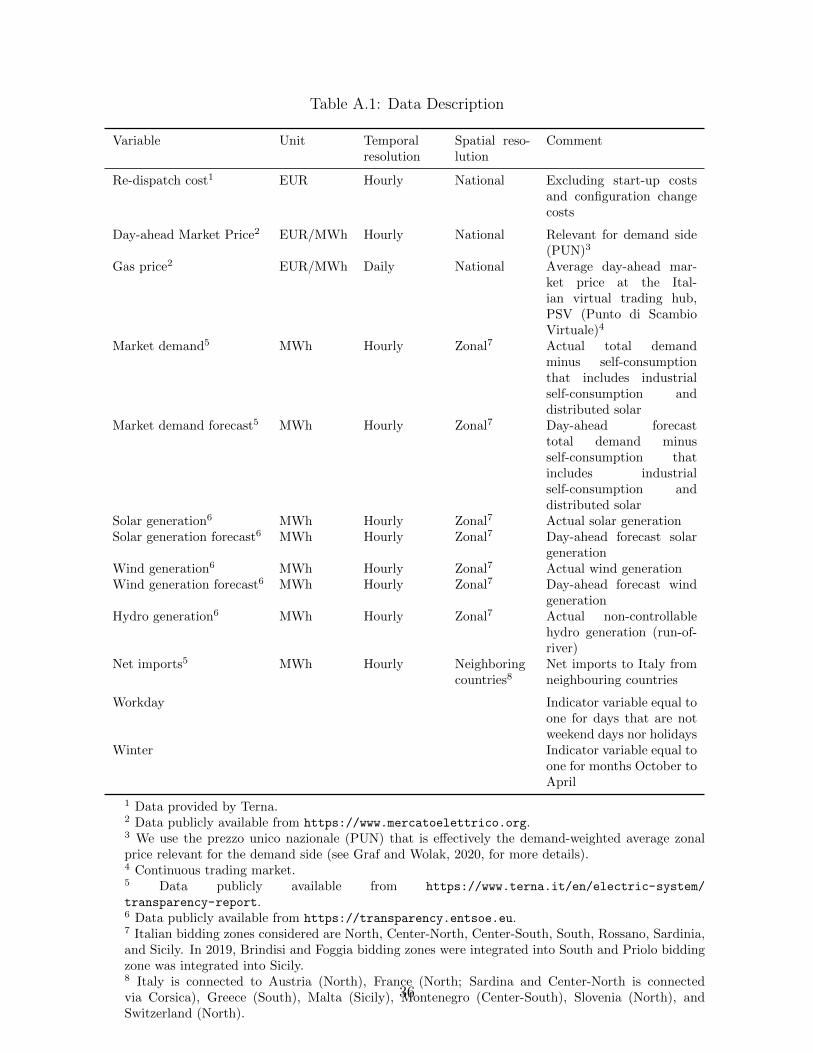
Table A.1: Data Description

Variable Unit Temporalresolution

Spatial reso-lution

Comment

Re-dispatch cost1 EUR Hourly National Excluding start-up costsand configuration changecosts

Day-ahead Market Price2 EUR/MWh Hourly National Relevant for demand side(PUN)3

Gas price2 EUR/MWh Daily National Average day-ahead mar-ket price at the Ital-ian virtual trading hub,PSV (Punto di ScambioVirtuale)4

Market demand5 MWh Hourly Zonal7 Actual total demandminus self-consumptionthat includes industrialself-consumption anddistributed solar

Market demand forecast5 MWh Hourly Zonal7 Day-ahead forecasttotal demand minusself-consumption thatincludes industrialself-consumption anddistributed solar

Solar generation6 MWh Hourly Zonal7 Actual solar generationSolar generation forecast6 MWh Hourly Zonal7 Day-ahead forecast solar

generationWind generation6 MWh Hourly Zonal7 Actual wind generationWind generation forecast6 MWh Hourly Zonal7 Day-ahead forecast wind

generationHydro generation6 MWh Hourly Zonal7 Actual non-controllable

hydro generation (run-of-river)

Net imports5 MWh Hourly Neighboringcountries8

Net imports to Italy fromneighbouring countries

Workday Indicator variable equal toone for days that are notweekend days nor holidays

Winter Indicator variable equal toone for months October toApril

1 Data provided by Terna.2 Data publicly available from https://www.mercatoelettrico.org.3 We use the prezzo unico nazionale (PUN) that is effectively the demand-weighted average zonalprice relevant for the demand side (see Graf and Wolak, 2020, for more details).4 Continuous trading market.5 Data publicly available from https://www.terna.it/en/electric-system/

transparency-report.6 Data publicly available from https://transparency.entsoe.eu.7 Italian bidding zones considered are North, Center-North, Center-South, South, Rossano, Sardinia,and Sicily. In 2019, Brindisi and Foggia bidding zones were integrated into South and Priolo biddingzone was integrated into Sicily.8 Italy is connected to Austria (North), France (North; Sardina and Center-North is connectedvia Corsica), Greece (South), Malta (Sicily), Montenegro (Center-South), Slovenia (North), andSwitzerland (North).

36

Table A.2: Descriptive Statistics

Variable Unit Location Count Mean Std Min Max

Re-dispatch cost EUR National 29,087 197,362 132,602 −107, 147 1,328,790

Day-ahead market price EUR/MWh National 29,087 54 16 0 170Gas Price EUR/MWh National 29,087 19 5 8 56

Net demand MWh North 29,087 9,930 3,964 561 23,633Net demand forecast MWh North 29,087 10,189 3,973 1,129 24,036

Net demand MWh Center-North 29,087 2,970 749 545 5,433Net demand forecast MWh Center-North 29,087 3,044 754 652 5,483

Net demand MWh Center-South 29,087 3,892 1,112 987 7,714Net demand forecast MWh Center-South 29,087 3,992 1,116 655 7,832

Net demand MWh South 29,087 1,523 1,110 −1, 979 4,672Net demand forecast MWh South 29,087 1,668 1,082 −2, 534 4,691

Net demand MWh Sardinia1 29,087 722 299 −559 1,532Net demand forecast MWh Sardinia1 29,087 734 297 −606 1,598

Net demand MWh Sicily 29,087 1,520 534 −163 3,550Net demand forecast MWh Sicily 29,087 1,565 528 −580 3,718

Net demand MWh Rossano2 29,087 −39 39 −180 0Net demand forecast MWh Rossano2 29,087 −40 36 −167 0

1 Net imports from Corsica are only considered in Sardinia’s net demand and net demand forecast.2 Limited production bidding zone with no demand.Notes: The data spans the period from January 1, 2017 to April 26, 2020. It is hourly data except for thegas price which is available on a daily basis. Missing values in the gas price time series and in any of thetime series used to construct zonal net demands and zonal net demand forecasts are linearly interpolated.

Table C.1: Optimal Hyper-parameters

Hyper-parameter Optimal value Possible values

Activation function ReLU ReLU, Tanh, SigmoidLearning rate 0.006161 Min: 1e-4; Max: 1e-2; “log-sampling”Dropout 0.1 0.1, 0.2, . . . , 0.5n1 48 16, 32, 48n2 48 16, 32, 48

37