Machine Learning for OR & FEIntroduction to Classification Algorithms

Martin HaughDepartment of Industrial Engineering and Operations Research

Columbia UniversityEmail: martin.b.haugh@gmail.com

Some of the figures in this presentation are taken from "An Introduction to Statistical Learning, withapplications in R" (Springer, 2013) with permission from the authors: G. James, D. Witten, T. Hastie

and R. Tibshirani (JWHT).Additional References: Chapter 4 of JWHT, Bishop’s PRML and HTF’s TESL.

OutlineIntroduction to Classificationk-Nearest NeighborsModel Fitting and AssessmentOptimal Bayes ClassifierNaive BayesClassification Using Linear RegressionLinear Discriminant Analysis (LDA)Assessing the Performance of a ClassifierQuadratic Discriminant Analysis (QDA)Logistic RegressionFeature Space Expansion With Basis FunctionsA Comparison of Classification MethodsAppendix: Reduced-Rank LDAAppendix: Adaptive k-Nearest Neighbors

2 (Section 0)

What is Classification?Goal is to predict a categorical outcome from a vector of inputs

- inputs can be quantitative, ordinal, or categorical- inputs could also be images, speech, text, networks, temporal data, spatial

data etc.

Classification algorithms require inputs to be encoded in quantitative form- can result in very high dimensional problems!

Simplest and most common type of classification is binary classification- email classification: spam or not spam?- sentiment analysis

- is the movie review good or bad?- is this good news for the stock or bad news?

- fraud detection- revenue management: will a person buy or not?- medical diagnosis: does a patient have a disease or not?- will somebody vote for Obama or not?- is somebody a terrorist or not?

But also have classification problems with multiple categories.3 (Section 1)

What is Classification?Classification often used as part of a decision support system.

There are many(!) different classification algorithms- will cover many of the best known algorithms- but will not have time to cover all of them such as neural networks,

ensemble methods etc.- will cover support vector machines later in the course.

Most classification algorithms can be categorized as generative or discriminative.Classification algorithms learn a classifier using training data

- then used to predict category or class for new inputs or test data.

Will use X or x to denote vector of inputs and G or Y to denote category orclass.

4 (Section 1)

Generative Classification AlgorithmsGenerative methods focus on modeling P(X,G) and then use G(X) as a classifierwhere

G(X) := argmaxG

P(G|X) = argmaxG

P(X|G)P(G)∑i P(X|Gi)P(Gi)

(1)

= argmaxG

P(X|G)P(G)

Examples include linear discriminant analysis (LDA), quadratic discriminantanalysis (QDA) and naive Bayes.

LDA and QDA assume Gaussian densities for P(X|G).

Naive Bayes assumesP(X|G) =

∏j

P(Xj |G)

so the features are independent conditional on G.- a strong and generally unrealistic assumption but naive Bayes still often

works very well in practice.5 (Section 1)

Discriminative Classification AlgorithmsDiscriminative methods focus on modeling P(G|X) directly

- examples include least squares or regression-based classifiers, logisticregression and Bayesian logistic regression.

Discriminative methods may also focus on minimizing the expected classificationerror directly without making any assumptions regarding P(X,G) or P(G|X).

Examples include:classification treesk-nearest neighborssupport vector machines (SVMs)(deep) neural networks.

6 (Section 1)

k-Nearest Neighborsk-nearest neighbors (k-NN) is a very simple classification algorithm.Given a new data-point, x, that needs to be classified, we find the k nearestneighbors of x and use majority voting of these neighbors to classify x.Need a metric to measure distance between data-points

- easy for quantitative variables and also straightforward for ordinal variables- generally a good idea (why?) to standardize features so they have mean 0

and variance 1

But constructing a metric not so straightforward for other variables includingcategorical variables, text documents, images, etc.

- choice of metric can be very important in these situations.

k is usually chosen by using separate training and test sets, or via cross-validation- to be covered soon.

Despite its simplicity, k-NN often works very well in practice but can becomputationally expensive to classify new points.k-NN’s can also be used for regression – k-NN regression

7 (Section 2)

k-Nearest Neighbors

A Demo of k-Nearest Neighbors by Antal van den Bosch

8 (Section 2)

Kernel Classificationk-NN gives equal weight to all k nearest neighbors but it may make more senseto give more weight to the closest neighbors –leads to kernel classification.

With kernel classification every training point, xi , gets a vote of K (x, xi) whenclassifying a new point, x.

e.g. A Gaussian-type kernel takes the form

K (x, xi) = e−d(x,xi)/σ2

where d(x, xi) is a distance measure between x and xi .

Question: What happens as σ →∞?

Question: What happens as σ → 0?

9 (Section 2)

Model AssessmentGoal of model selection: choose the model with the best predictions on new data.

Complex models generally fit a given training set better than less complex models- follows since more complex models have more flexibility- but often results in over-fitting in which case the fitted complex model does

not generalize well.

This is related to the bias-variance decomposition that we saw earlier when westudied regression.

Training error refers to classification error on the data-set that was used to trainthe classifier.

Test error refers to classification error on a new or holdout data-set that was notused to train the classifier

- provides an estimate of generalization error.

10 (Section 3)

Training Error Versus Test Error

Figure taken from Ben Taskar’s web-site at U Penn.

Training error generally declines as model complexity increases. Why?However, true error, i.e. test or generalization error, tends to decrease for a whileand then increase as it begins to over-fit the data.

11 (Section 3)

Approaches to Control Over-FittingMany approaches used to control over-fitting:

The Akaike information criterion (AIC) and Bayesian information criterion(BIC) penalize the effective # of parameters

- used in MLE settings when we can compute effective # of parameters.

Bayesian models control over-fitting naturally by modeling parameters asrandom variables

- estimation in these models therefore implicitly accounts for parameteruncertainty

- Bayesian models are very popular in statistics and ML.

Regularization approaches that explicitly penalize parameter magnitudesalong with the misclassification or prediction error in the objective function.Smaller magnitude parameters preferred to larger magnitude parameterswith degree of regularization controlled via a regularization parameter, λ.e.g. ridge regression solves

minβ

{12 ‖y− Xβ‖2 + λ · 1

2 ‖β‖22

}.

12 (Section 3)

Approaches to Control Over-FittingA standard approach is to use training, validation and test sets.

Another very useful technique is cross-validation- often the tool of choice- and also used to choose regularization parameters; e.g. λ in ridge regression.

For now will restrict ourselves to the training, validation and test set approach- will consider cross-validation later.

13 (Section 3)

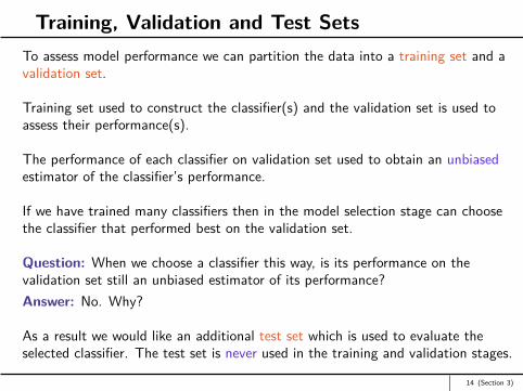
Training, Validation and Test SetsTo assess model performance we can partition the data into a training set and avalidation set.

Training set used to construct the classifier(s) and the validation set is used toassess their performance(s).

The performance of each classifier on validation set used to obtain an unbiasedestimator of the classifier’s performance.

If we have trained many classifiers then in the model selection stage can choosethe classifier that performed best on the validation set.

Question: When we choose a classifier this way, is its performance on thevalidation set still an unbiased estimator of its performance?Answer: No. Why?

As a result we would like an additional test set which is used to evaluate theselected classifier. The test set is never used in the training and validation stages.

14 (Section 3)

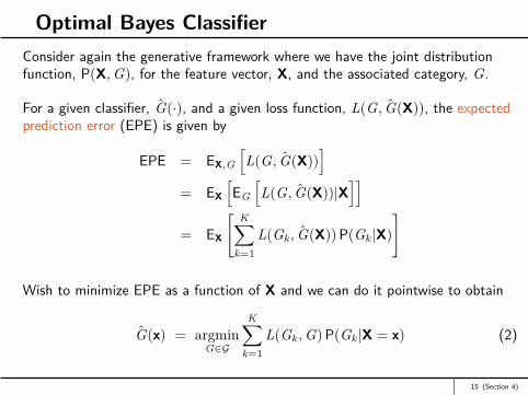
Optimal Bayes ClassifierConsider again the generative framework where we have the joint distributionfunction, P(X,G), for the feature vector, X, and the associated category, G.

For a given classifier, G(·), and a given loss function, L(G, G(X)), the expectedprediction error (EPE) is given by

EPE = EX,G

[L(G, G(X))

]= EX

[EG

[L(G, G(X))|X

]]= EX

[ K∑k=1

L(Gk , G(X)) P(Gk |X)]

Wish to minimize EPE as a function of X and we can do it pointwise to obtain

G(x) = argminG∈G

K∑k=1

L(Gk ,G) P(Gk |X = x) (2)

15 (Section 4)

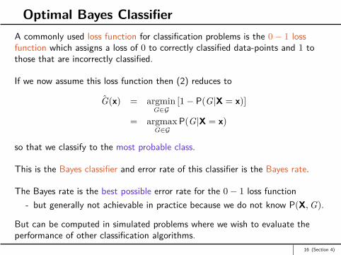
Optimal Bayes ClassifierA commonly used loss function for classification problems is the 0− 1 lossfunction which assigns a loss of 0 to correctly classified data-points and 1 tothose that are incorrectly classified.

If we now assume this loss function then (2) reduces to

G(x) = argminG∈G

[1− P(G|X = x)]

= argmaxG∈G

P(G|X = x)

so that we classify to the most probable class.

This is the Bayes classifier and error rate of this classifier is the Bayes rate.

The Bayes rate is the best possible error rate for the 0− 1 loss function- but generally not achievable in practice because we do not know P(X,G).

But can be computed in simulated problems where we wish to evaluate theperformance of other classification algorithms.

16 (Section 4)

Naive BayesRecall naive Bayes is a generative classifier that estimates P(X,G) and assumes

P(X|G) =∏

jP(Xj |G) (3)

so the features are independent conditional on G.

Since P(X,G) = P(X|G)P(G), naive Bayes estimates P(G) and the P(Xj |G)’sseparately via MLE and then classifies according to

G(x) = argmaxG∈G

P(G|X = x)

= argmaxG∈G

P(G)P(x|G)

= argmaxG∈G

P(G)∏

iP(xi |G)

Assumption (3) is strong and generally unrealistic- but when X is high-dimensional and categorical estimating P(X,G) is

generally (why?) not possible- so assumption (3) makes estimation much easier and naive Bayes still often

works very well in practice!17 (Section 5)

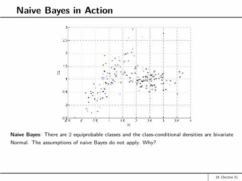
Naive Bayes in Action

Naive Bayes: There are 2 equiprobable classes and the class-conditional densities are bivariateNormal. The assumptions of naive Bayes do not apply. Why?

18 (Section 5)

Naive Bayes in Action

Naive Bayes: The contours of the fitted class-conditional densities. These densities are alsoassumed to be bivariate Normal. The naive Bayes classifier is given by the red curve.

19 (Section 5)

Naive Bayes and Text ClassificationNaive Bayes often works well when the data cannot support a more complexclassifier – this is the bias-variance decomposition again.Has been very successful in text classification or sentiment analysis

- e.g. is an email spam or not?

But how would you encode an email into a numerical input vector?A simple and common way to do this is via the bag-of-words model

- completely ignores the ordering of the words- stop-words such as “the”, “and”, “of”, “about” etc. are thrown out- words such as “walk”, “walking”, “walks” etc. all identified as “walk”

Email classification then done by assuming a given email comes from either a“spam” bag or a “non-spam”bag

- naive Bayes assumes P(spam|X) ∝ P(spam)∏

word∈email P(word|spam).

Bag-of-words also often used in document retrieval and classification- leads to the term-document matrix- also then need a measure of similarity between documents, e.g. cosine

distance possibly in TF-IDF version of term-document matrix.20 (Section 5)

Classification Using Linear RegressionThe 1-of-K encoding scheme uses K binary response variables to encode eachdata-point with

Yk ={

1, if G = k0, otherwise.

Linear regression approach to classification fits a linear regression with Yk as theresponse variable

- so K different linear regressions are performed.

Let fk(x) denote the fitted regression when Yk is the response variable. Classifierthen given by

G(x) := argmaxk∈G

fk(x)

so we simply classify to the largest component.

21 (Section 6)

Cons of Doing Classification Via RegressionLacks robustness to outliers like all least squares methods.

Masking is a major problem when there is more than two classes– not too surprising given that least-squares solutions correspond to MLE

estimates for conditional Gaussian distributions and not conditional Bernoullidistributions.

Figures on slides (26) and (44) demonstrate this masking phenomenon.

According to HTF all polynomial terms up to degree K − 1 might be needed toavoid this masking problem.

Masking not an issue with other classification techniques that we consider.

22 (Section 6)

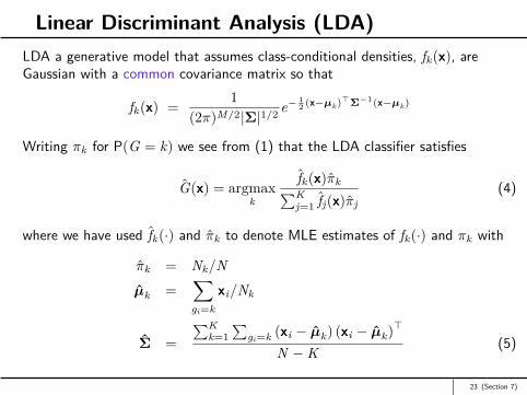
Linear Discriminant Analysis (LDA)LDA a generative model that assumes class-conditional densities, fk(x), areGaussian with a common covariance matrix so that

fk(x) = 1(2π)M/2|Σ|1/2 e− 1

2 (x−µk)>Σ−1(x−µk)

Writing πk for P(G = k) we see from (1) that the LDA classifier satisfies

G(x) = argmaxk

fk(x)πk∑Kj=1 fj(x)πj

(4)

where we have used fk(·) and πk to denote MLE estimates of fk(·) and πk with

πk = Nk/Nµk =

∑gi=k

xi/Nk

Σ =∑K

k=1∑

gi=k (xi − µk) (xi − µk)>

N −K (5)

23 (Section 7)

Linear Discriminant Analysis (LDA)Can also calculate log-ratio between two classes, k and l, to get

log P(G = k|X = x)P(G = l|X = x) = log πk

πl− 1

2 (µk + µl)> Σ

−1(µk − µl)

+ x>Σ−1

(µk − µl) (6)

Based on (6) can define the linear discriminant functions

δk(x) := x>Σ−1

µk + log πk −12 µ>k Σ

−1µk︸ ︷︷ ︸

kth intercept

(7)

for k = 1, . . . ,K .

LDA classifier of (4) then reduces to

G(x) = argmaxk

δk(x).

24 (Section 7)

Linear Discriminant Analysis (LDA)When there are just 2 classes it can be shown the linear regression and LDAclassifiers only differ in their intercepts

- not true for K > 2.

But since LDA is based on Gaussian assumptions and linear regression makes noprobabilistic assumptions, Hastie et al. suggest choosing the intercepts in (7) tominimize the classification error

- they report this works well in practice.

LDA does not suffer from the masking problem of linear regression.

25 (Section 7)

Figure 4.2 from HTF: The data come from three classes in R2 and are easily separated bylinear decision boundaries. The right plot shows the boundaries found by linear discriminantanalysis. The left plot shows the boundaries found by linear regression of the indicator responsevariables. The middle class is completely masked (never dominates).

−4 −2 0 2 4

−4

−2

02

4

−4 −2 0 2 4

−4

−2

02

4

X1X1

X2

X2

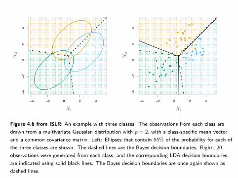
Figure 4.6 from ISLR: An example with three classes. The observations from each class aredrawn from a multivariate Gaussian distribution with p = 2, with a class-specific mean vectorand a common covariance matrix. Left: Ellipses that contain 95% of the probability for each ofthe three classes are shown. The dashed lines are the Bayes decision boundaries. Right: 20observations were generated from each class, and the corresponding LDA decision boundariesare indicated using solid black lines. The Bayes decision boundaries are once again shown asdashed lines.

The Default Data from ISLRISLR use LDA to obtain a classification rule for default / non-default on the basisof: (i) credit card balance and (ii) student status.

There were 10,000 training samples and the overall default rate was 3.33%.

The training error rate of LDA was 2.75%. But how good is this?

- note training error rate will usually be biased low and therefore lower thantest / generalization error

- for comparison, how well does the useless classifier that always predictsnon-default do?

We are often interested in breaking out the (training) error rate into the twopossible types of error:

1. False positives

2. False negatives.

This leads to the so-called confusion matrix.28 (Section 8)

The Confusion Matrix

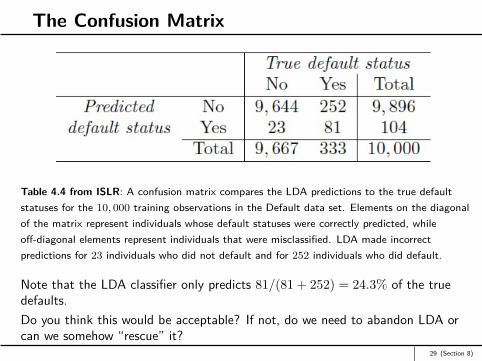
Table 4.4 from ISLR: A confusion matrix compares the LDA predictions to the true defaultstatuses for the 10, 000 training observations in the Default data set. Elements on the diagonalof the matrix represent individuals whose default statuses were correctly predicted, whileoff-diagonal elements represent individuals that were misclassified. LDA made incorrectpredictions for 23 individuals who did not default and for 252 individuals who did default.

Note that the LDA classifier only predicts 81/(81 + 252) = 24.3% of the truedefaults.Do you think this would be acceptable? If not, do we need to abandon LDA orcan we somehow “rescue” it?

29 (Section 8)

The Confusion Matrix for a Different Threshold

Table 4.5 from ISLR: A confusion matrix compares the LDA predictions to the true defaultstatuses for the 10, 000 training observations in the Default data set, using a modified thresholdvalue that predicts default for any individuals whose posterior default probability exceeds 20%.

We can rescue LDA by simply adjusting the threshold to emphasize one type oferror over another.In Table 4.5 we “predict“ default if the LDA model has

Prob (default = Yes |X = x) > 0.2.

What happens the overall training error rate with this new rule? Do we care?30 (Section 8)

The Tradeoff from Modifying the Threshold

0.0 0.1 0.2 0.3 0.4 0.5

0.0

0.2

0.4

0.6

Threshold

Err

or

Rate

Figure 4.7 from ISLR: For the Default data set, error rates are shown as a function of thethreshold value for the posterior probability that is used to perform the assignment. The blacksolid line displays the overall error rate. The blue dashed line represents the fraction ofdefaulting customers that are incorrectly classified, and the orange dotted line indicates thefraction of errors among the non-defaulting customers.

Domain specific knowledge required to decide on appropriate threshold- the ROC curve often used for this task.

31 (Section 8)

ROC Curve

False positive rate

Tru

e p

ositiv

e r

ate

0.0 0.2 0.4 0.6 0.8 1.0

0.0

0.2

0.4

0.6

0.8

1.0

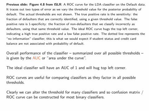
Previous slide: Figure 4.8 from ISLR: A ROC curve for the LDA classifier on the Default data.It traces out two types of error as we vary the threshold value for the posterior probability ofdefault. The actual thresholds are not shown. The true positive rate is the sensitivity: thefraction of defaulters that are correctly identified, using a given threshold value. The falsepositive rate is 1-specificity: the fraction of non-defaulters that we classify incorrectly asdefaulters, using that same threshold value. The ideal ROC curve hugs the top left corner,indicating a high true positive rate and a low false positive rate. The dotted line represents the“no information” classifier; this is what we would expect if student status and credit cardbalance are not associated with probability of default.

Overall performance of the classifier – summarized over all possible thresholds –is given by the AUC or “area under the curve”.

The ideal classifier will have an AUC of 1 and will hug top left corner.

ROC curves are useful for comparing classifiers as they factor in all possiblethresholds.

Clearly we can alter the threshold for many classifiers and so confusion matrix /ROC curve can be constructed for most binary classifiers.

Quadratic Discriminant Analysis (QDA)Drop equal covariance assumption and obtain quadratic discriminant functions

δk(x) := −12 log |Σk | − −

12 (x− µk)> Σ

−1k (x− µk) + log πk

QDA classifier is thenG(x) = argmax

kδk(x)

So decision boundaries between each pair of classes then given by quadraticfunctions of x.

LDA using linear and quadratic features generally gives similar results to QDA- QDA generally preferred due to greater flexibility at the cost of more

parameters to estimate.

LDA and QDA are popular and successful classifiers- probably because of the bias-variance decomposition and because the data

can often ”only support simple decision boundaries”.

34 (Section 9)

LDA with Quadratic Predictors v QDA

Figure 4.6 from HTF: Two methods for fitting quadratic boundaries. The left plot shows thequadratic decision boundaries for the data in Figure 4.1 (obtained using LDA in thefive-dimensional space X1, X2, X1X2, X2

1 , X22 ). The right plot shows the quadratic decision

boundaries found by QDA. The differences are small, as is usually the case.

35 (Section 9)

LDA v LDA with Quadratic Predictors

Figure 4.1 from HTF: The left plot shows some data from three classes, with linear decisionboundaries found by linear discriminant analysis. The right plot shows quadratic decisionboundaries. These were obtained by finding linear boundaries in the five-dimensional space X1,X2, X1X2,X2

1 , X22 . Linear inequalities in this space are quadratic inequalities in the original

space.36 (Section 9)

LDA v QDA

−4 −2 0 2 4

−4

−3

−2

−1

01

2

−4 −2 0 2 4

−4

−3

−2

−1

01

2

X1X1

X2

X2

Figure 4.9 from ISLR: Left: The Bayes (purple dashed), LDA (black dotted), and QDA (greensolid) decision boundaries for a two-class problem with Σ1 = Σ2. The shading indicates theQDA decision rule. Since the Bayes decision boundary is linear, it is more accuratelyapproximated by LDA than by QDA. Right: Details are as given in the left-hand panel, exceptthat Σ1 6= Σ2. Since the Bayes decision boundary is non-linear, it is more accuratelyapproximated by QDA than by LDA.

Note that LDA is superior (why?!) when true boundary is (close to) linear.37 (Section 9)

Logistic RegressionTwo possible classes encoded as y ∈ {0, 1} and assume

P(y = 1|x,w) =exp

(w>x

)1 + exp (w>x)

where w an m + 1-parameter vector and first element of x is the constant 1.

Follows that

P(y = 0|x,w) = 1− P(y = 1|x,w) = 11 + exp (w>x) .

Given N independently distributed data-points can write likelihood as

L(w) =N∏

i=1pi(w)yi (1− pi(w))1−yi

where pi(w) := P(yi = 1|xi ,w). Obtain w by maximizing the log-likelihood

l(w) =N∑

i=1

(yiw>xi − log

(1 + exp(w>xi)

))(8)

38 (Section 10)

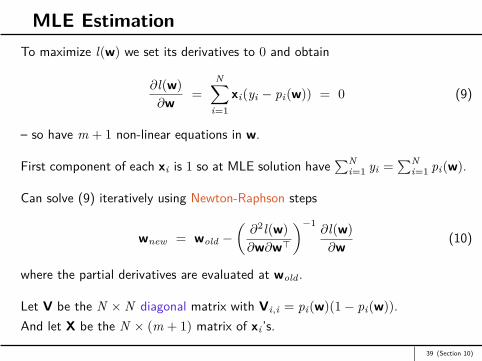
MLE EstimationTo maximize l(w) we set its derivatives to 0 and obtain

∂l(w)∂w =

N∑i=1

xi(yi − pi(w)) = 0 (9)

– so have m + 1 non-linear equations in w.

First component of each xi is 1 so at MLE solution have∑N

i=1 yi =∑N

i=1 pi(w).

Can solve (9) iteratively using Newton-Raphson steps

wnew = wold −(∂2l(w)∂w∂w>

)−1∂l(w)∂w (10)

where the partial derivatives are evaluated at wold .

Let V be the N ×N diagonal matrix with Vi,i = pi(w)(1− pi(w)).And let X be the N × (m + 1) matrix of xi ’s.

39 (Section 10)

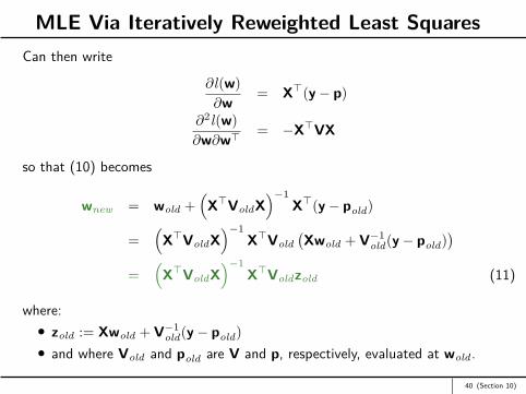
MLE Via Iteratively Reweighted Least SquaresCan then write

∂l(w)∂w = X>(y− p)

∂2l(w)∂w∂w> = −X>VX

so that (10) becomes

wnew = wold +(X>VoldX

)−1X>(y− pold)

=(X>VoldX

)−1X>Vold

(Xwold + V−1

old(y− pold))

=(X>VoldX

)−1X>Voldzold (11)

where:zold := Xwold + V−1

old(y− pold)and where Vold and pold are V and p, respectively, evaluated at wold .

40 (Section 10)

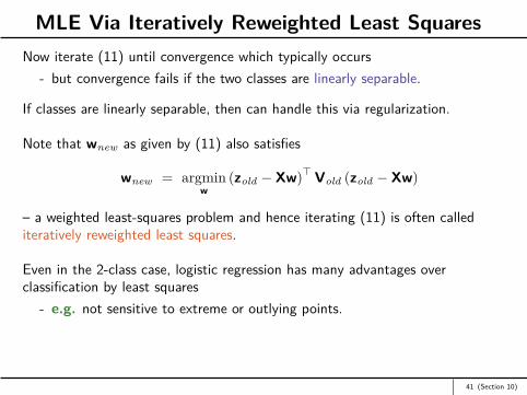
MLE Via Iteratively Reweighted Least SquaresNow iterate (11) until convergence which typically occurs

- but convergence fails if the two classes are linearly separable.

If classes are linearly separable, then can handle this via regularization.

Note that wnew as given by (11) also satisfies

wnew = argminw

(zold − Xw)>Vold (zold − Xw)

– a weighted least-squares problem and hence iterating (11) is often callediteratively reweighted least squares.

Even in the 2-class case, logistic regression has many advantages overclassification by least squares

- e.g. not sensitive to extreme or outlying points.

41 (Section 10)

−4 −2 0 2 4 6 8

−8

−6

−4

−2

0

2

4

−4 −2 0 2 4 6 8

−8

−6

−4

−2

0

2

4

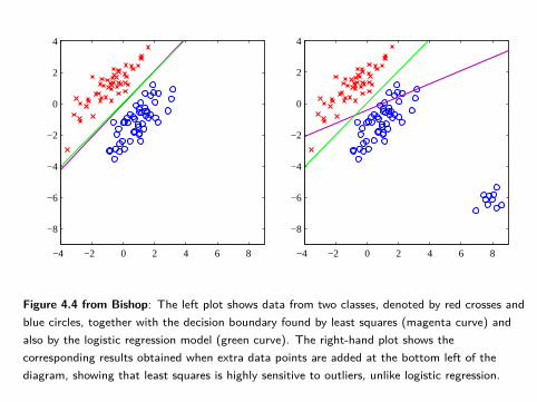
Figure 4.4 from Bishop: The left plot shows data from two classes, denoted by red crosses andblue circles, together with the decision boundary found by least squares (magenta curve) andalso by the logistic regression model (green curve). The right-hand plot shows thecorresponding results obtained when extra data points are added at the bottom left of thediagram, showing that least squares is highly sensitive to outliers, unlike logistic regression.

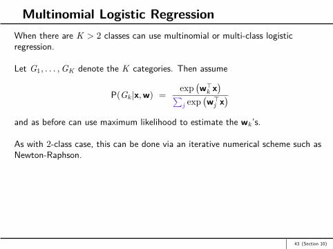
Multinomial Logistic RegressionWhen there are K > 2 classes can use multinomial or multi-class logisticregression.

Let G1, . . . ,GK denote the K categories. Then assume

P(Gk |x,w) =exp

(w>k x

)∑j exp

(w>j x

)and as before can use maximum likelihood to estimate the wk ’s.

As with 2-class case, this can be done via an iterative numerical scheme such asNewton-Raphson.

43 (Section 10)

−6 −4 −2 0 2 4 6−6

−4

−2

0

2

4

6

−6 −4 −2 0 2 4 6−6

−4

−2

0

2

4

6

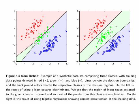
Figure 4.5 from Bishop: Example of a synthetic data set comprising three classes, with trainingdata points denoted in red (×), green (+), and blue (◦). Lines denote the decision boundaries,and the background colors denote the respective classes of the decision regions. On the left isthe result of using a least-squares discriminant. We see that the region of input space assignedto the green class is too small and so most of the points from this class are misclassified. On theright is the result of using logistic regressions showing correct classification of the training data.

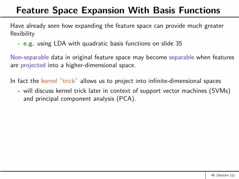
Feature Space Expansion With Basis FunctionsHave already seen how expanding the feature space can provide much greaterflexibility

- e.g. using LDA with quadratic basis functions on slide 35

Non-separable data in original feature space may become separable when featuresare projected into a higher-dimensional space.

In fact the kernel ”trick” allows us to project into infinite-dimensional spaces- will discuss kernel trick later in context of support vector machines (SVMs)

and principal component analysis (PCA).

45 (Section 11)

x1

x2

−1 0 1

−1

0

1

φ1

φ2

0 0.5 1

0

0.5

1

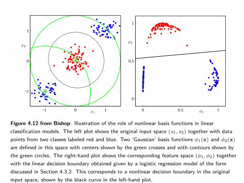
Figure 4.12 from Bishop: Illustration of the role of nonlinear basis functions in linearclassification models. The left plot shows the original input space (x1, x2) together with datapoints from two classes labeled red and blue. Two ‘Gaussian’ basis functions φ1(x) and φ2(x)are defined in this space with centers shown by the green crosses and with contours shown bythe green circles. The right-hand plot shows the corresponding feature space (φ1, φ2) togetherwith the linear decision boundary obtained given by a logistic regression model of the formdiscussed in Section 4.3.2. This corresponds to a nonlinear decision boundary in the originalinput space, shown by the black curve in the left-hand plot.

A Comparison of Classification Methods

KNN−1 KNN−CV LDA Logistic QDA

0.2

50

.30

0.3

50

.40

0.4

5

SCENARIO 1

KNN−1 KNN−CV LDA Logistic QDA

0.1

50

.20

0.2

50

.30

SCENARIO 2

KNN−1 KNN−CV LDA Logistic QDA

0.2

00

.25

0.3

00

.35

0.4

00

.45

SCENARIO 3

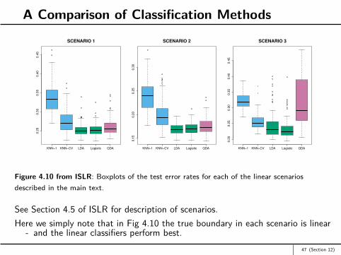
Figure 4.10 from ISLR: Boxplots of the test error rates for each of the linear scenariosdescribed in the main text.

See Section 4.5 of ISLR for description of scenarios.Here we simply note that in Fig 4.10 the true boundary in each scenario is linear

- and the linear classifiers perform best.47 (Section 12)

A Comparison of Classification Methods

KNN−1 KNN−CV LDA Logistic QDA

0.3

00

.35

0.4

0SCENARIO 4

KNN−1 KNN−CV LDA Logistic QDA

0.2

00

.25

0.3

00

.35

0.4

0

SCENARIO 5

KNN−1 KNN−CV LDA Logistic QDA

0.1

80

.20

0.2

20

.24

0.2

60

.28

0.3

00

.32

SCENARIO 6

Figure 4.11 from ISLR: Boxplots of the test error rates for each of the non-linear scenariosdescribed in the main text.

Here we note that in Fig 4.11 the true boundary in each scenario is non-linear- and the linear classifiers are no longer the best.

Aside: KNN-CV refers to KNN with K chosen via cross-validation- to be studied soon!

48 (Section 12)

Appendix: Reduced-Rank LDARecall our LDA analysis but now rewrite log-ratio in (6) as

log P(G = k|X = x)P(G = l|X = x) = log πk

πl− 1

2 (x− µk)> Σ−1

(x− µk)

+ 12 (x− µl)

> Σ−1

(x− µl) (12)

Now let SW := Σ = UDU> be the eigen decomposition of Σ where:U is an m ×m orthornormal matrixD is a diagonal matrix of the positive eigen values of Σ.

Consider now a change of variable with x∗ := D−1/2U>x- so that variance-covariance matrix of x∗ is the identity matrix- often called sphering the data.

Also implies µ∗k := D−12 U>µk are now the estimated class centroids and

(x− µk)> S−1W (x− µk) = ‖x∗ − µ∗k‖

22 .

49 (Section 13)

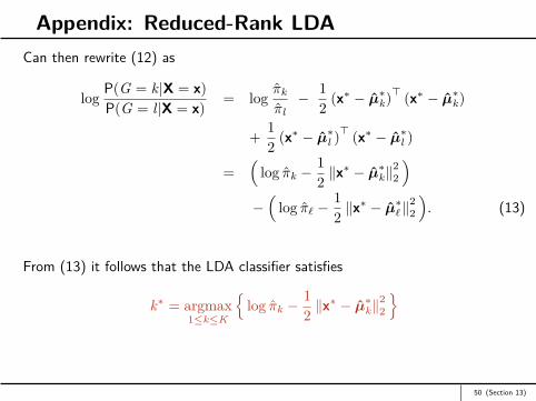
Appendix: Reduced-Rank LDACan then rewrite (12) as

log P(G = k|X = x)P(G = l|X = x) = log πk

πl− 1

2 (x∗ − µ∗k)> (x∗ − µ∗k)

+ 12 (x∗ − µ∗l )> (x∗ − µ∗l )

=(

log πk −12 ‖x

∗ − µ∗k‖22

)−(

log π` −12 ‖x

∗ − µ∗`‖22

). (13)

From (13) it follows that the LDA classifier satisfies

k∗ = argmax1≤k≤K

{log πk −

12 ‖x

∗ − µ∗k‖22

}

50 (Section 13)

Appendix: LDA in Spherical Coordinates

−2 2 6

−2

0

2

4

−2 2 6

−2

0

2

4

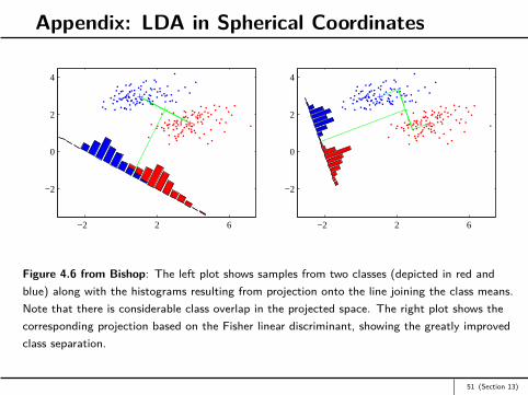
Figure 4.6 from Bishop: The left plot shows samples from two classes (depicted in red andblue) along with the histograms resulting from projection onto the line joining the class means.Note that there is considerable class overlap in the projected space. The right plot shows thecorresponding projection based on the Fisher linear discriminant, showing the greatly improvedclass separation.

51 (Section 13)

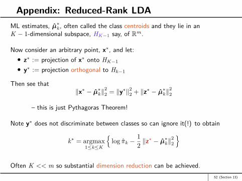
Appendix: Reduced-Rank LDAML estimates, µ∗k , often called the class centroids and they lie in anK − 1-dimensional subspace, HK−1 say, of Rm.

Now consider an arbitrary point, x∗, and let:z∗ := projection of x∗ onto HK−1

y∗ := projection orthogonal to Hk−1

Then see that‖x∗ − µ∗k‖

22 = ‖y∗‖2

2 + ‖z∗ − µ∗k‖22

– this is just Pythagoras Theorem!

Note y∗ does not discriminate between classes so can ignore it(!) to obtain

k∗ = argmax1≤k≤K

{log πk −

12 ‖z

∗ − µ∗k‖22

}

Often K << m so substantial dimension reduction can be achieved.52 (Section 13)

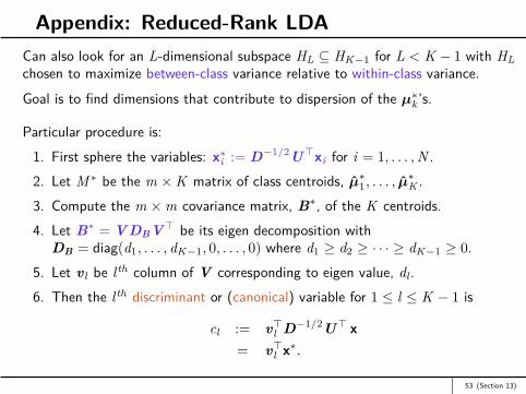
Appendix: Reduced-Rank LDACan also look for an L-dimensional subspace HL ⊆ HK−1 for L < K − 1 with HLchosen to maximize between-class variance relative to within-class variance.

Goal is to find dimensions that contribute to dispersion of the µ∗k ’s.

Particular procedure is:1. First sphere the variables: x∗i := D−1/2U>xi for i = 1, . . . ,N .2. Let M ∗ be the m ×K matrix of class centroids, µ∗1, . . . , µ

∗K .

3. Compute the m ×m covariance matrix, B∗, of the K centroids.4. Let B∗ = V DBV> be its eigen decomposition with

DB = diag(d1, . . . , dK−1, 0, . . . , 0) where d1 ≥ d2 ≥ · · · ≥ dK−1 ≥ 0.5. Let vl be lth column of V corresponding to eigen value, dl .6. Then the lth discriminant or (canonical) variable for 1 ≤ l ≤ K − 1 is

cl := v>l D−1/2U> x= v>l x∗.

53 (Section 13)

Appendix: Reduced-Rank LDAThese steps can be understood via:

A principal components analysis (PCA)Or by solving a generalized eigen-value problem

- the original approach of Fisher.

Discriminant function can now be written as

k∗ = argmax1≤k≤K

{log(πk)− 1

2

m∑`=1

(v>l (x∗ − µ∗k)

)2}

On Slide 55 we plot pairs of canonical variates for the “vowel data” of HTF.

Notice that the lower the coordinates, the more spread out the centroids.

54 (Section 13)

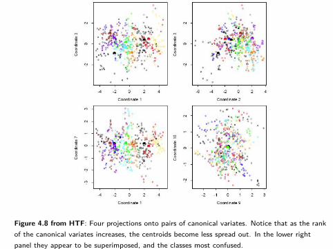
Figure 4.8 from HTF: Four projections onto pairs of canonical variates. Notice that as the rankof the canonical variates increases, the centroids become less spread out. In the lower rightpanel they appear to be superimposed, and the classes most confused.

Appendix: Classification Using Discriminant Subspaces

Projecting class centroids onto 2- or 3-dimensional discriminant subspaces aids invisualization.

However, also possible that performing classification in HL (instead of HK−1) forL < K − 1 might yield a superior classifier. Why?

Figure on Slide 57 plots training and test error against L, the dimension of thediscriminant subspace used for LDA, using the vowel data of Hastie et al.

- K = 11 classes and M = 10 variables- we see that L = 2 yields the best test error.

Figure on Slide 58 shows the corresponding optimal classification regions in H2.

56 (Section 13)

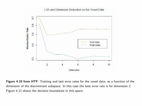
Figure 4.10 from HTF: Training and test error rates for the vowel data, as a function of thedimension of the discriminant subspace. In this case the best error rate is for dimension 2.Figure 4.11 shows the decision boundaries in this space.

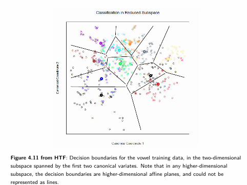
Figure 4.11 from HTF: Decision boundaries for the vowel training data, in the two-dimensionalsubspace spanned by the first two canonical variates. Note that in any higher-dimensionalsubspace, the decision boundaries are higher-dimensional affine planes, and could not berepresented as lines.

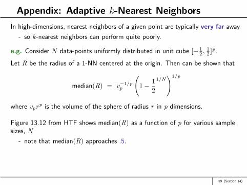
Appendix: Adaptive k-Nearest NeighborsIn high-dimensions, nearest neighbors of a given point are typically very far away

- so k-nearest neighbors can perform quite poorly.

e.g. Consider N data-points uniformly distributed in unit cube [− 12 ,

12 ]p.

Let R be the radius of a 1-NN centered at the origin. Then can be shown that

median(R) = v−1/pp

(1− 1

2

1/N)1/p

where vprp is the volume of the sphere of radius r in p dimensions.

Figure 13.12 from HTF shows median(R) as a function of p for various samplesizes, N

- note that median(R) approaches .5.

59 (Section 14)

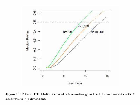
Figure 13.12 from HTF: Median radius of a 1-nearest-neighborhood, for uniform data with Nobservations in p dimensions.

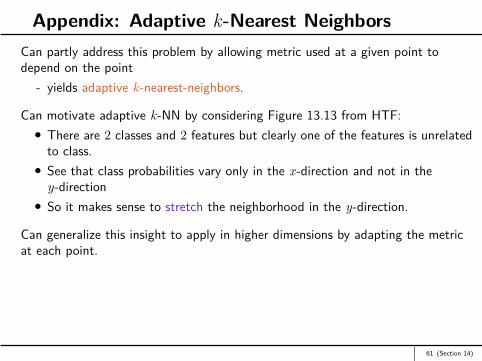
Appendix: Adaptive k-Nearest NeighborsCan partly address this problem by allowing metric used at a given point todepend on the point

- yields adaptive k-nearest-neighbors.

Can motivate adaptive k-NN by considering Figure 13.13 from HTF:There are 2 classes and 2 features but clearly one of the features is unrelatedto class.See that class probabilities vary only in the x-direction and not in they-directionSo it makes sense to stretch the neighborhood in the y-direction.

Can generalize this insight to apply in higher dimensions by adapting the metricat each point.

61 (Section 14)

Figure 13.13 from HTF: The points are uniform in the cube, with the vertical line separatingclass red and green. The vertical strip denotes the 5-nearest-neighbor region using only thehorizontal coordinate to find the nearest-neighbors for the target point (solid dot). The sphereshows the 5-nearest-neighbor region using both coordinates, and we see in this case it hasextended into the class-red region (and is dominated by the wrong class in this instance).

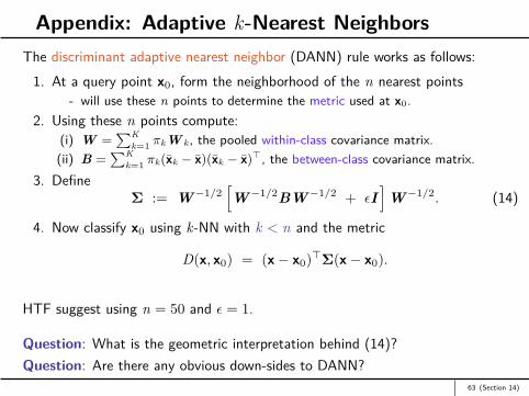
Appendix: Adaptive k-Nearest NeighborsThe discriminant adaptive nearest neighbor (DANN) rule works as follows:

1. At a query point x0, form the neighborhood of the n nearest points- will use these n points to determine the metric used at x0.

2. Using these n points compute:(i) W =

∑Kk=1 πkW k , the pooled within-class covariance matrix.

(ii) B =∑K

k=1 πk(xk − x)(xk − x)>, the between-class covariance matrix.3. Define

Σ := W−1/2[W−1/2BW−1/2 + εI

]W−1/2. (14)

4. Now classify x0 using k-NN with k < n and the metric

D(x, x0) = (x− x0)>Σ(x− x0).

HTF suggest using n = 50 and ε = 1.

Question: What is the geometric interpretation behind (14)?Question: Are there any obvious down-sides to DANN?

63 (Section 14)

Figure 13.14 from HTF: Neighborhoods found by the DANN procedure, at various query points(centers of the crosses). There are two classes in the data, with one class surrounding theother. 50 nearest-neighbors were used to estimate the local metrics. Shown are the resultingmetrics used to form 15-nearest-neighborhoods.

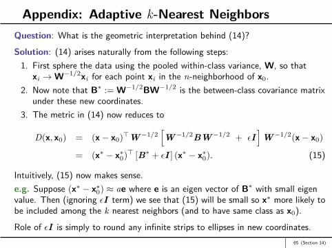
Appendix: Adaptive k-Nearest NeighborsQuestion: What is the geometric interpretation behind (14)?

Solution: (14) arises naturally from the following steps:1. First sphere the data using the pooled within-class variance, W, so that

xi →W−1/2xi for each point xi in the n-neighborhood of x0.2. Now note that B∗ := W−1/2BW−1/2 is the between-class covariance matrix

under these new coordinates.3. The metric in (14) now reduces to

D(x, x0) = (x− x0)>W−1/2[W−1/2BW−1/2 + εI

]W−1/2(x− x0)

= (x∗ − x∗0)> [B∗ + εI ] (x∗ − x∗0). (15)

Intuitively, (15) now makes sense.e.g. Suppose (x∗ − x∗0) ≈ ae where e is an eigen vector of B∗ with small eigenvalue. Then (ignoring εI term) we see that (15) will be small so x∗ more likely tobe included among the k nearest neighbors (and to have same class as x0).

Role of εI is simply to round any infinite strips to ellipses in new coordinates.65 (Section 14)