machine learning for numerical stabilization of advection

Machine learning for numerical stabilization of

advection-diffusion PDEs

Courses: Numerical Analysis for Partial Differential Equations -Advanced Programming for Scientific Computing

Margherita Guido, Michele Vidulis

Suprevisor: prof. Luca Dede

09/09/2019

Contents

1 Introduction 5

2 Problem: SUPG stabilization and Isogeometric analysis 7

2.1 Advection-diffusion problem . . . . . . . . . . . . . . . . . . . . . . . 7

2.1.1 Weak formulation and numerical discretization using FE . . . 8

2.2 SUPG stabilization . . . . . . . . . . . . . . . . . . . . . . . . . . . . 9

2.2.1 A Variational Multiscale (VMS) approach . . . . . . . . . . . 9

2.3 Isogeometric analysis . . . . . . . . . . . . . . . . . . . . . . . . . . . 11

2.3.1 B-Spline basis functions . . . . . . . . . . . . . . . . . . . . . 11

2.3.2 B-Spline geometries . . . . . . . . . . . . . . . . . . . . . . . 11

2.3.3 NURBS basis functions . . . . . . . . . . . . . . . . . . . . . 12

2.3.4 NURBS as trial space for the solution of the Advection-Diffusionproblem . . . . . . . . . . . . . . . . . . . . . . . . . . . . . . 12

2.3.5 Mesh refinement and convergence results . . . . . . . . . . . . 12

3 Artificial Neural Networks 15

3.1 Structure of an Artificial Neural Network . . . . . . . . . . . . . . . 15

3.1.1 Notation . . . . . . . . . . . . . . . . . . . . . . . . . . . . . . 15

3.1.2 Design of an ANN . . . . . . . . . . . . . . . . . . . . . . . . 16

3.2 Universal approximation property . . . . . . . . . . . . . . . . . . . . 17

3.3 Backpropagation and training . . . . . . . . . . . . . . . . . . . . . . 17

3.3.1 Some terminology . . . . . . . . . . . . . . . . . . . . . . . . 17

3.3.2 The learning algorithm . . . . . . . . . . . . . . . . . . . . . 18

4 A Neural Network to learn the stabilization parameter 21

4.1 Our Neural Network scheme . . . . . . . . . . . . . . . . . . . . . . . 21

4.2 Mathematical formulation of the problem . . . . . . . . . . . . . . . 22

4.3 Expected results . . . . . . . . . . . . . . . . . . . . . . . . . . . . . 24

4.4 Implementation aspects . . . . . . . . . . . . . . . . . . . . . . . . . 24

4.4.1 Keras . . . . . . . . . . . . . . . . . . . . . . . . . . . . . . . 24

4.4.2 C++ libraries . . . . . . . . . . . . . . . . . . . . . . . . . . . 25

5 Isoglib and OpenNN 27

5.1 Structure of IsoGlib . . . . . . . . . . . . . . . . . . . . . . . . . . . 27

5.1.1 Definition of the problem . . . . . . . . . . . . . . . . . . . . 27

5.1.2 Main steps in solving process . . . . . . . . . . . . . . . . . . 28

5.1.3 Export and visualization of the results . . . . . . . . . . . . . 28

5.2 Structure of OpenNN . . . . . . . . . . . . . . . . . . . . . . . . . . 28

5.2.1 Uses of the library . . . . . . . . . . . . . . . . . . . . . . . . 28

5.2.2 Vectors and matrices . . . . . . . . . . . . . . . . . . . . . . . 29

5.2.3 DataSet class . . . . . . . . . . . . . . . . . . . . . . . . . . . 29

5.2.4 NeuralNetwork class . . . . . . . . . . . . . . . . . . . . . . . 30

5.2.5 TrainingStrategy class . . . . . . . . . . . . . . . . . . . . . 30

5.2.6 LossIndex class . . . . . . . . . . . . . . . . . . . . . . . . . 30

5.2.7 OptimizationAlgorithm class . . . . . . . . . . . . . . . . . 31

5.2.8 Backpropagation . . . . . . . . . . . . . . . . . . . . . . . . . 31

3

4 CONTENTS

6 Implementation: interface of OpenNN and IsoGlib 356.1 SUPG solver in IsoGlib . . . . . . . . . . . . . . . . . . . . . . . . . 35

6.1.1 Our test class: SUPGdata . . . . . . . . . . . . . . . . . . . . 356.1.2 SUPGLocalMatrix class . . . . . . . . . . . . . . . . . . . . . 36

6.2 New OpenNN classes . . . . . . . . . . . . . . . . . . . . . . . . . . . 366.2.1 IsoglibInterface class . . . . . . . . . . . . . . . . . . . . . 366.2.2 Customized loss function: OutputFunction class . . . . . . . 38

6.3 SUPG example in OpenNN . . . . . . . . . . . . . . . . . . . . . . . 426.3.1 Data of the problem . . . . . . . . . . . . . . . . . . . . . . . 426.3.2 Training . . . . . . . . . . . . . . . . . . . . . . . . . . . . . . 426.3.3 Testing . . . . . . . . . . . . . . . . . . . . . . . . . . . . . . 43

7 Numerical Tests 457.1 Training of the network . . . . . . . . . . . . . . . . . . . . . . . . . 467.2 Prediction of the SUPG parameter . . . . . . . . . . . . . . . . . . . 477.3 Analysis of the results . . . . . . . . . . . . . . . . . . . . . . . . . . 487.4 L2 error trend in a different PDE . . . . . . . . . . . . . . . . . . . . 50

8 Conclusions 53

Bibliography 55

Chapter 1

Introduction

High-order numerical methods for the approximation of advection–diffusion PDEsbased on Galerkin finite element may be affected from numerical instabilities, whichoccur as spurious oscillations and compromise the solution accuracy.

A stabilized and strongly consistent method named Streamline Upwind Petrov-Galerkin Method (SUPG) can be obtained by adding a further term to the Galerkinapproximation (see (HB82) and (Q17, chap.13)). This term includes an elementwisestabilization parameter that should be carefully determined, since an exact formuladefining its optimal value is still lacking. Through the years, several approximationsof this coefficient have been proposed: we present the simplest and most used, tryingto frame the ideas that lead to their definition (see (HSF18) and (C97)).

The aim of our work is to exploit the universal approximation power of the Arti-ficial Neural Networks to reconstruct a suitable approximation of such stabilizationparameter. We train an Artificial Neural Network, implemented inside the C++ li-brary OpenNN (OpenNN), so that, once the parameters characterizing the problemand its discretization are known, we predict an optimal value of the stabilizationparameter. To train our network we developed a customized loss function that re-quires several numerical resolution of the stabilized PDE, for which we employ aC++ library (IsoGlib), based on Isogeometric analysis (CHB09).

We start presenting the problem in its theoretical framework, describing thefamily of PDE equations we want to solve, some instability issues and how they canbe confined, constructing a theoretical background for this problem. In Chapter 2we will also introduce Isogeometric Analysis, the technique that will be used to solvenumerically the PDEs problems. Chapter 3 is devoted to the description of Artifi-cial Neural Networks and the algorithm involved in their training, with particularattention to the description of how we designed our customized Neural Network. InChapter 4 our original problem is formalized, with the purpose of putting in com-munication the world of EDPs with the one of ANNs, and describing the effort wemade to realize our project. Chapter 5 contains a description of the libraries used forthe implementation (OpenNN and IsoGlib), while in Chapter 6 we will present theclasses we developed to interface them. Numerical results are presented in Chapter7 to demonstrate the performance of this network-based technique and results arecritically discussed comparing them with the known formulas. At the end (Chapter8) , possible further developments of this technique are presented. Indeed we startfrom the implementation of a neural network that works on a simplified version ofthe PDE problem but, once this network is tested, we already have in mind how tocustomize it for more complicated problems.

5

Chapter 2

Problem: SUPG stabilizationand Isogeometric analysis

2.1 Advection-diffusion problem

Advection–diffusion PDEs (see (Q17, chap.13)) are used to model a wide range ofphenomena such as semiconductor devices modeling, magnetostatics and electro-static flows, heat and mass-transfer and flows in porous media related to oil andgroundwater applications. The linear advection–diffusion equation on a domainΩ Ď Rd “ 2, 3 is a boundary value problem of the form:

#

Lu “ ´divpµpxq∇uq ` bpxq ¨∇u “ f in Ω

u “ 0 on BΩ(2.1)

where µpxq and bpxq are respectively the diffusion and advection coefficent. Inmany practical applications, the diffusion term ´divpµpxq∇uq is dominated by thetransport term bpxq ¨ ∇u. In such cases the solution can give rise to boundarylayers, namely regions, generally close to the boundary of Ω, where the solutionis characterized by strong gradients. From a numerical point of view, solvingthese types of advection-dominated problems using Galerkin Finite Element methodleads to nonphysical oscillation near the boundary layers. An example of this phe-nomenon can be seen in 2.1, obtained using the following data µ “ 10´4, β “ r1, 1sin Ω “ p0, 1q2 and a forcing term f such that the exact solution is given by:

uex “ ´atan´

px´0.5q2`py´0.5q2´ 116?

µ

¯

A challenging problem is to find numerical

scheme that works well in all types of regime, without increasing the computationaleffort to solve the PDE problem.

The goal of this project is to find an innovative way to code the SUPG stabi-lization method, exploiting Artificial Neural Networks to select the best value of thestabilization parameter.

7

8CHAPTER 2. PROBLEM: SUPG STABILIZATION AND ISOGEOMETRIC ANALYSIS

Figure 2.1: Numerical oscillations in 2D

2.1.1 Weak formulation and numerical discretization using FE

Let V “ H10 pΩq be the reference Sobolev space, let a : V ˆ V Ñ R be the bilinear

form

apu, vq “

ż

Ωµ∇u ¨∇v dΩ`

ż

Ωb ¨∇uv dΩ

and let F : V Ñ R be the linear functional

F pvq “

ż

Ωfv dΩ

The weak formulation of problem (2.1) reads

Find u P V : apu, vq “ F pvq @v P V (2.2)

The existence of a unique solution follows from the Lax-Milgram Theorem.By choosing a suitable family tVh, h ą 0u of finite dimensional subspaces of V

we can state the Galerkin formulation of the problem:

Find uh P Vh : apuh, vhq “ F pvhq @vh P Vh (2.3)

that is well posed thanks to the previous analysis. Moreover the Galerkin errorinequality gives:

‖u´ uh‖V ďM

αinfvhPVh ‖v ´ vh‖V (2.4)

where α “ µ0

1`C2Ω

and M “ ‖µ‖L8pΩq ` ‖b‖L8pΩq are the coercivity and continuity

constant of ap¨, ¨q, given µ0 the lower bound for the diffusive coefficient µ.By the definitions of α and M , the upper-bounding constant M

α of the errorbecomes larger (and, correspondingly, the estimate 2.4 meaningless) as the ratio‖b‖L8pΩq‖µ‖L8pΩq

grows and tends to infinity. This happens in the advection dominated

regime: in such cases the Galerkin method can give inaccurate solutions, presentingnumerical oscillations.

The dimensionless coefficient that measures the relation between transport anddiffusion is called Peclet number and is defined as

Pe “|b|h

2µ(2.5)

being h the dimension of the mesh. To understand the significance of the Pecletnumber it can be useful to look at the 1D problem:

#

´µu2 ` bu1 “ 0, 0 ă x ă 1

up0q “ 0, up1q “ 1

2.2. SUPG STABILIZATION 9

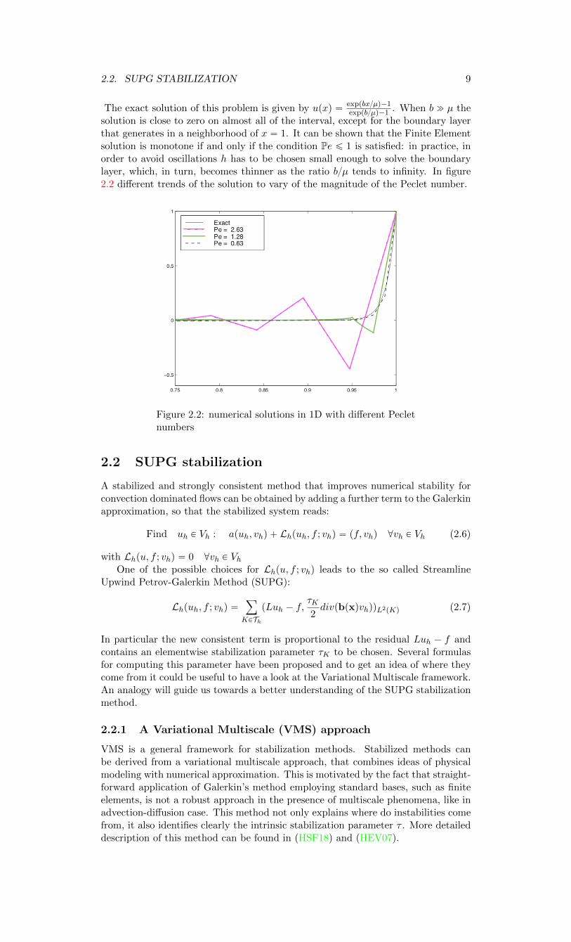
The exact solution of this problem is given by upxq “ exppbxµq´1exppbµq´1 . When b " µ the

solution is close to zero on almost all of the interval, except for the boundary layerthat generates in a neighborhood of x “ 1. It can be shown that the Finite Elementsolution is monotone if and only if the condition Pe ď 1 is satisfied: in practice, inorder to avoid oscillations h has to be chosen small enough to solve the boundarylayer, which, in turn, becomes thinner as the ratio bµ tends to infinity. In figure2.2 different trends of the solution to vary of the magnitude of the Peclet number.

Figure 2.2: numerical solutions in 1D with different Pecletnumbers

2.2 SUPG stabilization

A stabilized and strongly consistent method that improves numerical stability forconvection dominated flows can be obtained by adding a further term to the Galerkinapproximation, so that the stabilized system reads:

Find uh P Vh : apuh, vhq ` Lhpuh, f ; vhq “ pf, vhq @vh P Vh (2.6)

with Lhpu, f ; vhq “ 0 @vh P VhOne of the possible choices for Lhpu, f ; vhq leads to the so called Streamline

Upwind Petrov-Galerkin Method (SUPG):

Lhpuh, f ; vhq “ÿ

KPTh

pLuh ´ f,τK2divpbpxqvhqqL2pKq (2.7)

In particular the new consistent term is proportional to the residual Luh ´ f andcontains an elementwise stabilization parameter τK to be chosen. Several formulasfor computing this parameter have been proposed and to get an idea of where theycome from it could be useful to have a look at the Variational Multiscale framework.An analogy will guide us towards a better understanding of the SUPG stabilizationmethod.

2.2.1 A Variational Multiscale (VMS) approach

VMS is a general framework for stabilization methods. Stabilized methods canbe derived from a variational multiscale approach, that combines ideas of physicalmodeling with numerical approximation. This is motivated by the fact that straight-forward application of Galerkin’s method employing standard bases, such as finiteelements, is not a robust approach in the presence of multiscale phenomena, like inadvection-diffusion case. This method not only explains where do instabilities comefrom, it also identifies clearly the intrinsic stabilization parameter τ . More detaileddescription of this method can be found in (HSF18) and (HEV07).


The idea of the variational multiscale applied to problems that produce an in-accurate Galerkin solution is based on decomposing the solution in two terms. Anapproximation is made to determine one of them analytically, while the other oneis computed using Galerkin method, which will then be able to produce accuratesolutions.

In symbols, we write the exact solution u P V as the sum of uh and u˚ belong-ing respectively to the FE space Vh and to V ˚, which is any complement to it inV . Each VMS-type method depends on the way V ˚ is approximated. The samedecomposition is performed for the test functions.

Rewriting the weak formulation of the problem as

Find u P V : pLu, vq “ pf, vq @v P V (2.8)

where L is the second order differential operator corresponding to the advectiondiffusion equation, we can introduce the multiscale decomposition:

Find puh, u˚q P Vh ˆ V

˚ :

pLuh, vh ` v˚q ` pLu˚, vh ` v

˚q “ pf, vh ` v˚q @pvh, v

˚q P Vh ˆ V˚ (2.9)

By taking alternatively vh “ 0 and v˚ “ 0, we obtain the following system oftwo equations:

#

pLuh, vhq ` pLu˚, vhq “ pf, vhq @vh P Vh

pLuh, v˚q ` pLu˚, v˚q “ pf, v˚q @v˚ P V ˚

(2.10)

where the first equation is at grid scale while the second one at subgrid scale.The idea is, at first, to “solve” the subgrid scale equation approximating its

solution, then to substitute this solution in the grid scale equation.We rewrite the subgrid scale equation as:

pLu˚, v˚q “ pLuh ´ f, v˚q @v˚ P V ˚ (2.11)

which, in strong form, reads Lu˚ “ Luh ´ f . The expression for the infinitedimensional part of the solution follows:

u˚ “ L´1pLuh ´ fq

This solution results to be driven by Luh ´ f , that represents the residual of thesubgrid equation.

Now we make our approximation: since the inverse of the differential operatoris not easy to compute, we estimate it with the constant τ .

u˚ – τpLuh ´ fq (2.12)

Now we can substitute the approximation of u˚ in the grid scale equation:

pLuh, vhq ` pLpτpLuh ´ fqq, vhq “ pf, vhq @vh P Vh (2.13)

and, using the definition of L˚, adjoint operator of L, we get:

pLuh, vhq ` pτpLuh ´ fq, L˚vhq “ pf, vhq @vh P Vh (2.14)

Here we can see the analogy with the SUPG stabilization formulation where theadvective part of the differential operator L substitutes L˚ in 2.7. Indeed, thisformulation can be obtained with a similar procedure, leading to a stabilizationparameter τ strictly related to the approximate solution of the subproblem for u˚ PV ˚.

Using an advanced analysis based on, for example, the employment of Green’sfunction or maximum principle, several formulas for the approximation of tau canbe shown (see (HSF18, chap. 3.6)). In particular, for linear finite elements, τ canbe obtained as:

τ “h

2|b|pcothpPeq ´

1

Peq (2.15)

where Pe is the Peclet number defined in 2.5. This choice comes from the impositionof nodal exactness of the solution in 1D problems with uniform grids (see (C97)).Alternative formulas will be presented in section 4.3.

2.3. ISOGEOMETRIC ANALYSIS 11

2.3 Isogeometric analysis

Isogeometric Analysis ((CHB09),(Q17, chap.11)) – commonly abbreviated as IGA– is a technique for the spatial approximation of PDEs based on the so called isoge-ometric concept. Extensively developed in the last decade, IGA originally aimed atrestoring the centrality of the geometric representation of the computational domainin the numerical approximation of PDEs. In particular, it allows the exact repre-sentation of certain curved shapes, eliminating, for example in the case of a circularboundaries, the domain approximation from the sources of error. This approachconsiders Non-Rational Uniform B-Splines (NURBS) bases both for the construc-tion of the finite dimensional space and for the geometry representation. In this wayIGA gets perfectly integrated with CAD procedures that exploit the same kind offunctions.

We will provide a brief overview of NURBS–based IGA in the framework ofthe Galerkin method, starting from the definition of B–splines and NURBS basisfunctions and geometries. Then we will address the isogeometric concept and theapproximation properties of the Galerkin method.

2.3.1 B-Spline basis functions

B-splines are piecewise polynomials which are built from a linear combination ofbasis functions with local support and controlled continuity. They are built startingfrom a knot vector Ξ “ tξ1, ξ2, ..., ξn`p`1u, where p is the polynomial degree and nis the number of basis functions. The vector Ξ contains non-decreasing real values(possibly repeated) belonging to a parameter domain (usually r0, 1s). We indicateby mi the multiplicity of the i-th knot and we call element each of the intervalsdelimited by subsequent knots (leaving the possibility of having null size elementsin case of mi ě 1). We will consider only open knot vectors, meaning that first andlast nodes are taken with multiplicity p` 1.

A knot vector defines the set of basis functions through the following recursiverelation (Cox-de Boor formula)

Ni,0pξq “

#

1, ξ P rξi, ξi`1q

0, otherwise(2.16)

Ni,ppξq “ξ ´ ξiξi`1 ´ ξi

Ni,p´1pξq `ξi`p`1 ´ ξ

ξi`p`1 ´ ξi`1Ni`1,p´1pξq i “ 1, ..., n (2.17)

We indicated the i-th basis function of degree p as Ni,ppξq. All the basis functions arenon-negative, have a regularity degree at each knot which coincides with p´mi andare infinitely differentiable out of the knots. Moreover, each function has supportover p` 1 knots and shares the support with at most 2p` 1 other basis functions.A remarkable property of the set tNi,ppξqui for any fixed p is that it constitutes apartition of unity.

2.3.2 B-Spline geometries

Through a geometrical mapping, defined from the parametric domain into the physi-cal space Rd, B-Spline curves (or, more in general, surfaces and solids if as parameterspace Rk is chosen, with k ď d) can be defined starting from the basis functionspresented in the previous section. A set of control points belonging to the physicalspace, each one associated to a basis function, is needed too. Control points areindicated as tP iu

ni“1.

The B-Spline geometry φ : Ω Ñ Rd is defined as

φpξq “nÿ

i“1

P iNi,ppξq (2.18)

It is interesting to note that open knot vectors give rise to curves having extremacoinciding with the first and the last control points. It is not true, in general, thatthe other control points belong to the curve.


2.3.3 NURBS basis functions

B-Splines, being piecewise polynomials, does not ensure the exact representation ofconic sections. That is why NURBS are introduced.

To define the basis functions a set of real positive weights is needed: let’s indicateit with tw1, ..., wnu. The i´ th NURBS basis function of degree p is given by:

Ri,ppξq “Ni,ppξqwiW pξq

“Ni,ppξqwi

řnj“1Nj,ppξqwj

(2.19)

Note that Ri,p : Ω Ñ Rd is no more a piecewise polynomial; anyway, the letter p isstill used to indicate the degree of B-Splines from which NURBS are derived.

NURBS geometries can be generated with an analogous procedure to the oneused in the previous section.

2.3.4 NURBS as trial space for the solution of the Advection-Diffusion problem

The commonly indicated NURBS–based IGA relies on the very same NURBS basisfunctions first used to represent the computational domain of a PDE also to buildlater the finite dimensional trial space.

In standard finite elements it is the choice of the basis functions for the solutionthat conditions the meshing procedure. On the other hand, in isogeometric analysisthe basis is chosen to be suitable for the geometry, and then it is used for the solutionspace.

Let’s choose, in the Galerkin formulation (1.3), Vh as the space spanned by theNURBS basis functions:

Vh “ spantRi, uNhi“1

so that the Galerkin solution can be expressed as

uhpxq “Nhÿ

i“1

RiUi (2.20)

for some suitable coefficients Ui, known as control variables (also referred to asdegrees of freedom or DOFs). It can be shown that this produces a numericalsolution that converges to the exact one, since the NURBS basis functions satisfysome properties required by the Galerkin theory.

The NURBS basis is not an interpolatory basis as the finite element Lagrangianbasis. Indeed, if we assume that a control point P i lays in Ω, the value taken by theapproximate solution uh in such control point uhpP iq does not coincide in generalwith the corresponding control variable Ui. Moreover, some of the control pointsused to build the computational domain may even lay outside Ω; in those cases, theapproximate solution at these points is not defined.

2.3.5 Mesh refinement and convergence results

The convergence of the method is guaranteed by the theory of Galerkin methodsand isoparametric elements. The proof of the analogous result for classical finiteelements is complicated by the fact that it is hard to find suitable interpolationestimates using NURBS functions, because the basis functions are not polynomialand because they can have support over several elements. By introducing suitablefunctional spaces and deriving estimates on those spaces, an interpolation resultcan be obtained and it can be deduced that the order of convergence of the solutionobtained with isogeometric analysis using NURBS of degree p is the same as thatof classical finite elements of the same degree. In particular, provided the solutionand the domain are regular enough, the following estimates hold:

‖u´ uh‖L2 ď Chp`1 (2.21)

‖u´ uh‖H1 ď Chp (2.22)

2.3. ISOGEOMETRIC ANALYSIS 13

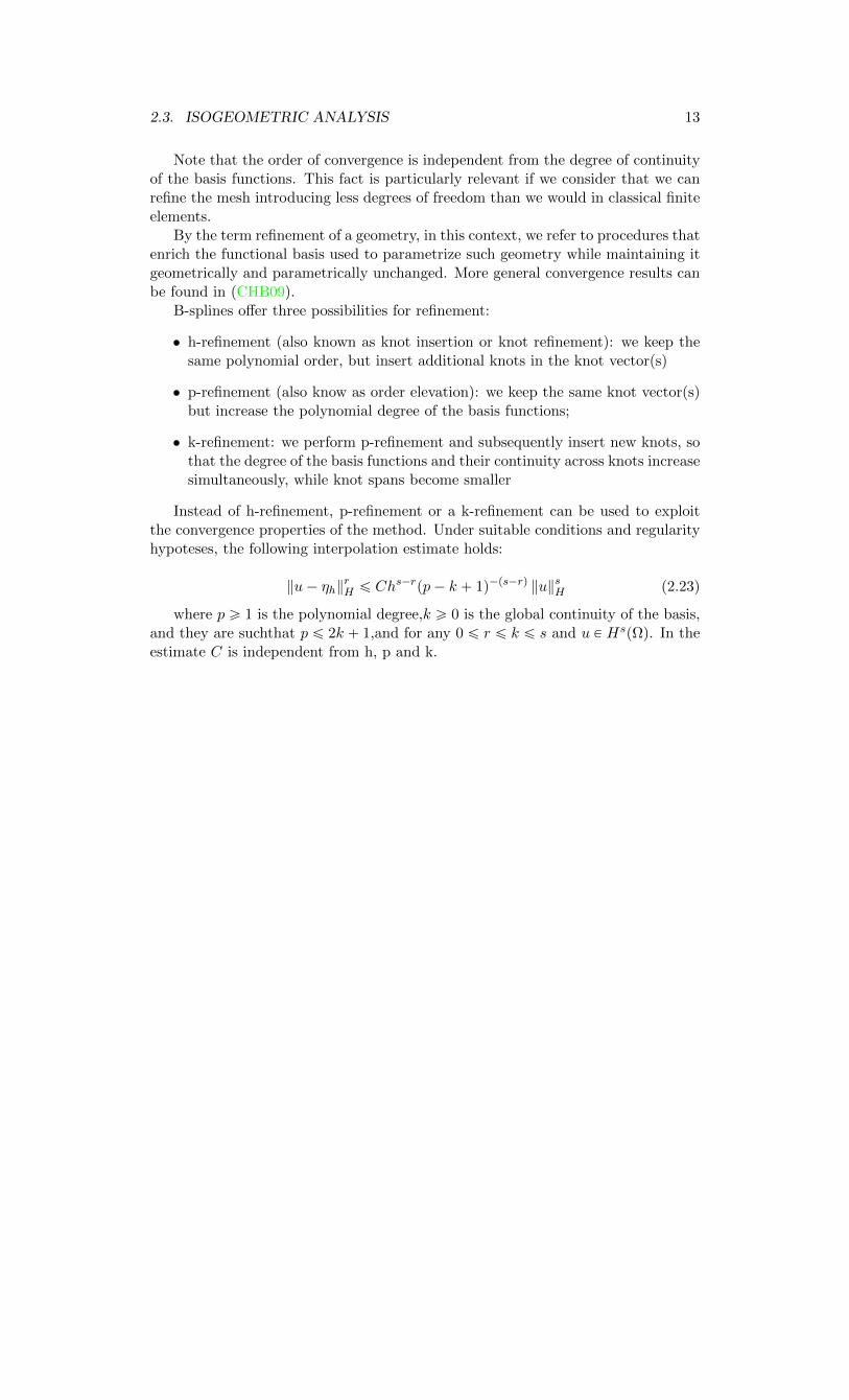
Note that the order of convergence is independent from the degree of continuityof the basis functions. This fact is particularly relevant if we consider that we canrefine the mesh introducing less degrees of freedom than we would in classical finiteelements.

By the term refinement of a geometry, in this context, we refer to procedures thatenrich the functional basis used to parametrize such geometry while maintaining itgeometrically and parametrically unchanged. More general convergence results canbe found in (CHB09).

B-splines offer three possibilities for refinement:

• h-refinement (also known as knot insertion or knot refinement): we keep thesame polynomial order, but insert additional knots in the knot vector(s)

• p-refinement (also know as order elevation): we keep the same knot vector(s)but increase the polynomial degree of the basis functions;

• k-refinement: we perform p-refinement and subsequently insert new knots, sothat the degree of the basis functions and their continuity across knots increasesimultaneously, while knot spans become smaller

Instead of h-refinement, p-refinement or a k-refinement can be used to exploitthe convergence properties of the method. Under suitable conditions and regularityhypoteses, the following interpolation estimate holds:

‖u´ ηh‖rH ď Chs´rpp´ k ` 1q´ps´rq ‖u‖sH (2.23)

where p ě 1 is the polynomial degree,k ě 0 is the global continuity of the basis,and they are suchthat p ď 2k ` 1,and for any 0 ď r ď k ď s and u P HspΩq. In theestimate C is independent from h, p and k.

Chapter 3

Artificial Neural Networks

In this chapter we will explain how Artificial Neural Networks (ANNs) work. Wewill describe their structure introducing the notation that will be used also in thefollowing chapter for the formalization of our problem and we will recall their fun-damental property of universal approximation of continuous functions (R96). Afterexplaining the meaning of some recurrent terms, we will describe the algorithm usedduring the training phase, highlighting the steps which are going to be modified byour original implementation.

3.1 Structure of an Artificial Neural Network

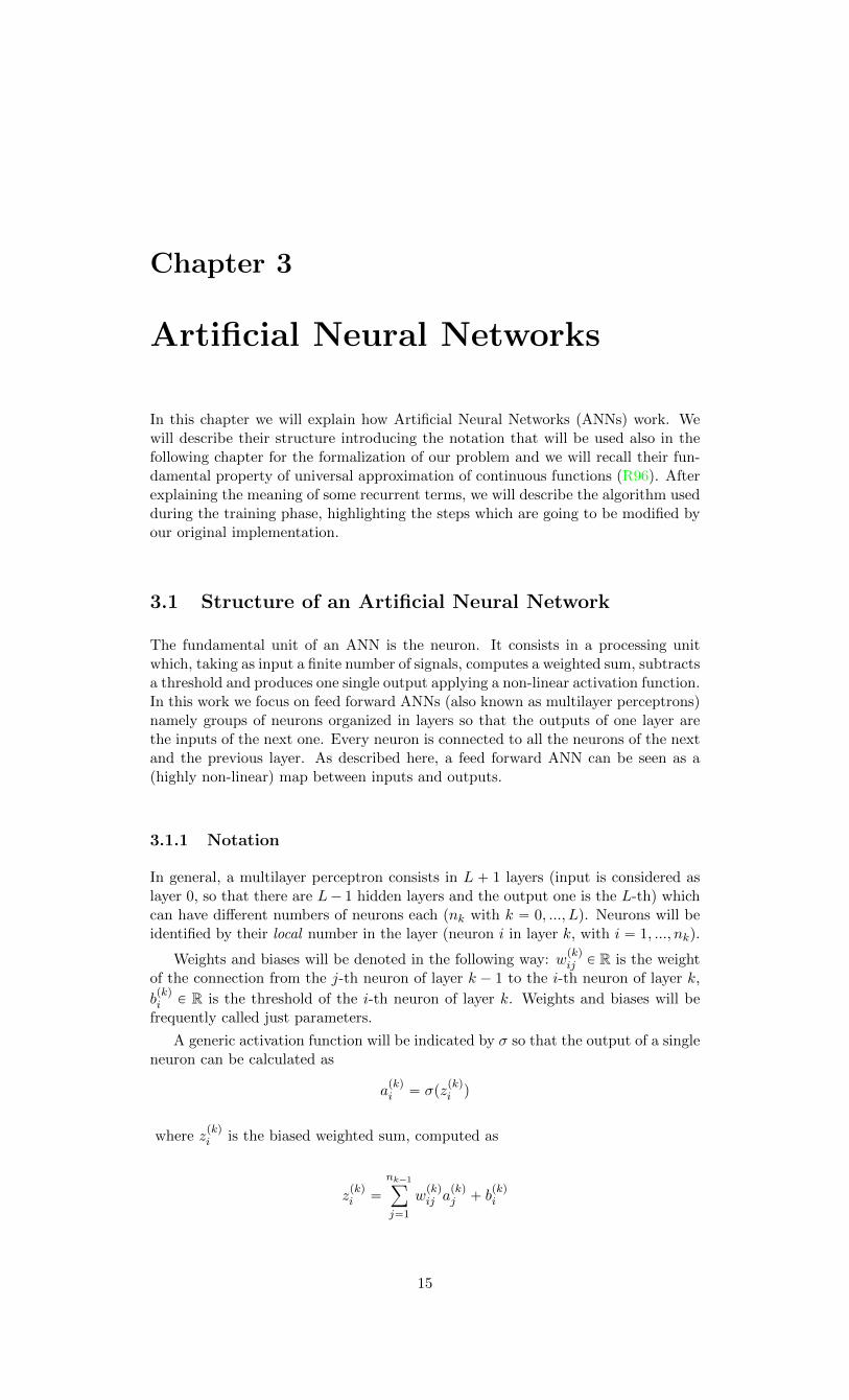
The fundamental unit of an ANN is the neuron. It consists in a processing unitwhich, taking as input a finite number of signals, computes a weighted sum, subtractsa threshold and produces one single output applying a non-linear activation function.In this work we focus on feed forward ANNs (also known as multilayer perceptrons)namely groups of neurons organized in layers so that the outputs of one layer arethe inputs of the next one. Every neuron is connected to all the neurons of the nextand the previous layer. As described here, a feed forward ANN can be seen as a(highly non-linear) map between inputs and outputs.

3.1.1 Notation

In general, a multilayer perceptron consists in L ` 1 layers (input is considered aslayer 0, so that there are L´ 1 hidden layers and the output one is the L-th) whichcan have different numbers of neurons each (nk with k “ 0, ..., L). Neurons will beidentified by their local number in the layer (neuron i in layer k, with i “ 1, ..., nk).

Weights and biases will be denoted in the following way: wpkqij P R is the weight

of the connection from the j-th neuron of layer k ´ 1 to the i-th neuron of layer k,

bpkqi P R is the threshold of the i-th neuron of layer k. Weights and biases will be

frequently called just parameters.

A generic activation function will be indicated by σ so that the output of a singleneuron can be calculated as

apkqi “ σpz

pkqi q

where zpkqi is the biased weighted sum, computed as

zpkqi “

nk´1ÿ

j“1

wpkqij a

pkqj ` b

pkqi

15

16 CHAPTER 3. ARTIFICIAL NEURAL NETWORKS

Figure 3.1: Neural network structure, and action of the i´ th neuron

3.1.2 Design of an ANN

Some features of an ANN, the ones which define its structure, have to be chosen apriori, before the training process takes place (actually, some of this characteristicscan be tuned during the model selection phase, which we will not describe being outof the scope of this project). For example, the number of hidden layers and the dis-tribution of neurons inside the ANN are two examples of so called hyperparameters,namely a group of parameters (that will not be updated during the training) whichnot only affects the performance of the ANN but also represents its actual definition.The number of layers and neurons which maximizes the learning capability of theANN depends on the specific application.

Another important design feature to be chosen is the set of activation functions.In this field there are few classical choices we will now present, remembering thatany Heaviside-like function mimicking the behavior of biological neurons can beaccepted. The most common activation functions are:

• hyperbolic tangent: sigmoidal function with output belonging to p´1, 1q

σpxq “ex ´ e´x

ex ` e´x

• logistic: sigmoidal function with output belonging to p0, 1q

σpxq “1

1` e´x

• rectified linear (relu): output is strictly positive

σpxq “

#

0 x ď 0

x x ą 0

• softplus: strictly monotone with output strictly positive

σpxq “ lnp1` exq

ANNs of the type described above can be employed in solving two kinds ofproblems: classification and approximation. The first one arises when there is apattern which needs to be identified, some features and some classes to which theobjects of the analysis belong. We will not go into the details of pattern recognitionsince our task falls under the second category. We only notice that proper activationfunctions have to be chosen to obtain as (discrete) output the classification of theinstance. Approximation tasks, instead, aim at recovering the continuous relationbetween inputs and outputs.

Note that, despite being the choice of the hyperparameters so important, thereare no universal rules to determine the best ANN setup to solve a generic problem.Anyway, the following fundamental result makes our effort justified.

3.2. UNIVERSAL APPROXIMATION PROPERTY 17

3.2 Universal approximation property

As we already pointed out, in an approximation problem an ANN can be seen as amap continuously linking in and out values. The following result (Cybenko, 1989.See (C89)) states that the set of feed forward ANNs with single hidden layer canapproximate any continuous function over a compact set.

Let σ : R Ñ R be a noncostant, bounded and continuous function (activationfunction). Let Im be the m-dimensional unit hypercube and CpImq the space ofreal-valued continuous functions on Im. Then the following theorem holds:

Theorem 1 @ε ą 0, @f P CpImq, DN P N, Dvi, bi P R, Dwi P Rm such that we maydefine

F pxq “Nÿ

i“1

viσpwTi x` bq

as an approximate realization of f, that is: |F pxq ´ fpxq| ă ε @x P Im.

The theorem can be reformulated in the framework of ANNs in the following way:

Theorem 2 Every ANN with a single hidden layer can approximate with arbitrarilysmall error any continuous function on a compact set, provided that a sufficientnumber of hidden neurons are employed.

3.3 Backpropagation and training

We will now describe the training algorithm, at first giving a rapid overview andthen, once the notation and some important terms are well understood, going intosome more technical details (see (R96, chap.7) for more detailed descriptions).

Learning, from the point of view of an ANN, means adapting to some sampleobservations (the training set), gaining in this way the ability to generalize andpredict results starting from inputs not included in the training set itself. The keyingredients for the learning phase are a loss function (which evaluates the currentperformance of the Neural Network) and an optimization algorithm (e.g. gradientdescent, which is responsible of finding the minimum of the loss).

The scheme of the algorithm is the following:

1. Weights and biases are randomly initialized.

2. Inputs are fed into the ANN and outputs are obtained forward-propagatingthe values; outputs are used to evaluate the loss function.

3. The gradient of the loss function with respect to every parameter is computed.

4. Weights and biases are updated according to the direction indicated by thegradient.

Steps 2, 3 and 4 are repeated until the algorithm stops because a terminationcondition is reached. Possible termination criteria adopted are the maximum num-ber of iterations, desired value of the loss function, time elapsed. Step 3 containsthe actual core of the algorithm and will be explained in detail in a while.

In the following section we will enumerate the most important concepts involvedin the training process, accompanying them with a brief explanation.

3.3.1 Some terminology

Loss function

Measures the performance of the ANN. Results obtained from the inputs are com-pared to targets through a suitable measure and the loss value summarizes thegoodness of the comparison. Classical examples are mean squared error measure(for approximation problems) and cross entropy (for classification).


Optimization algorithm

Needed to find the minimum of the loss function. Optimization algorithms can beclassified depending on two criteria: memory consumption and time to reach con-vergence. Usually the fastest ones need also more memory to be run: it’s the case ofLevenberg-Marquardt and quasi-Newton methods, which exploit the computationof second derivatives to accelerate convergence; gradient descent and conjugate gra-dient, instead, are better suited for optimization over big data sets, when memoryconsumption can become an issue.

Training set

It’s the set of instances (inputs and corresponding outputs) used to make the modellearn. Its values are fed into the Neural Network repeatedly until the predictedoutputs are close enough to the target values.

Validation (or selection) set

It is used during the learning phase too, but ANN parameters are not updated basedon its values. Inputs and targets are used to control overfitting: the loss computedon this data set (which contains values that the Neural Network meets for the firsttime) is compared to the one obtained with the training set; if the ANN performswell on training set but not on validation then overfitting happened and learningshould be stopped.

Testing set

Contains data used to test the performance of the ANN once it has been trained.

Epoch

Defines the time frame in which the whole data set in scanned once by the NeuralNetwork.

Batch

Usually, data instances are not processed one at a time; in fact, groups of inputsare chosen to calculate groups of outputs. The evaluation of the loss function takesinto account the results from the whole batch so that, during the update of theparameters, single values don’t spoil the generalization capability of the ANN.

Learning rate

States the magnitude of the decrease of the parameters during training. It can beconsidered the most important hyperparameter of an ANN, even if, differently fromthe layers and the neurons numbers, can be adapted during training.

3.3.2 The learning algorithm

The learning algorithm in its generality is called backpropagation. The idea isthe following: one of the parameters is slightly perturbed and the effect of thisperturbation over the value of the loss is observed. In this way the sensibility of theloss with respect to that specific parameter (namely: its derivative) is measured.Once the procedure is done for every parameter, the gradient of the loss function isknown and it is possible to update the parameters in order to reduce the loss valueduring the next iteration. In practice, the derivatives of the loss can be calculatedvia chain rule and this is the reason why the algorithm is named in this way.

To show how the differentiation process works in detail we need to select, withoutlosing generality, a specific loss function (from now on denoted by L ). Since we

3.3. BACKPROPAGATION AND TRAINING 19

used an approximation of an L2 norm in our implementation, (mean) squared errorcan be considered as the benchmark loss. Explicitly:

L “

nLÿ

i“1

papLqi ´ yiq

2looooomooooon

Ei

(3.1)

where yi, i “ 1, ..., nL are the target values (whose value is contained in the trainingset) corresponding to the nL outputs of the ANN, while Ei is the contribution tothe total error given by the i-th output.

Let’s analyze the algorithm in detail following the numeration of the steps in-troduced in the previous section. About steps 1 and 2 there are only a couple ofthings to be pointed out.

1. Parameters initialization: since the Neural Network is optimized to workwith signals of order zero, not only inputs have to be scaled but also the param-eters should respect some kind of constraint. That’s why, usually, initializationvalues are chosen randomly in the interval p´1, 1q.

2. Forward propagation: a batch of inputs is selected from the training setand processed by the ANN. Each neuron computes an affine transformation ofits (local) inputs applying its own activation function to the result. The valueof the local output of each neuron is saved for later use and, at the end of thepropagation, the global outputs of the Neural Network are available. They areused to evaluate the loss and check whether the ANN performances increased.

3. Backward propagation: here is where the gradient of the loss function iscalculated. Let’s start considering the simplest cases: the derivatives of theloss w.r.t. the weights of the connections between layer L ´ 1 and the layerof the outputs. Recalling the notation previously introduced, they can becomputed as:

BL

BwpLqij

“

nLÿ

i“1

BEi

BwpLqij

“

nLÿ

i“1

BEi

BapLqi

¨BapLqi

BzpLqi

¨BzpLqi

BwpLqij

(3.2)

with:BEi

BapLqi

“ 2papLqi ´ yiq (3.3)

BapLqi

BzpLqi

“ σ1pzpLqi q (3.4)

BzpLqi

BwpLqij

“ apL´1qj (3.5)

Note that, at this point, all the values in 3.3 are known thanks to the forwardpropagation performed in step 2.

Computing derivatives with respect to parameters belonging to previous layersis just a matter of applying the chain rule. We will show how it can be donefor a weight in the last but one layer; the procedure can then be generalizedto all the parameters of the ANN. In this case the derivative is:

BL

BwpL´1qij

“

nLÿ

t“1

BEt

BwpL´1qij

“

nLÿ

t“1

˜

BEt

BapLqt

¨BapLqt

BzpLqt

¨BzpLqt

BapL´1qj

¸

¨BapL´1qi

BzpL´1qi

¨BzpL´1qi

BwpL´1qij

(3.6)with:

BzpLqt

BapL´1qj

“ wpLqti (3.7)

and the value of the other terms understood from the previous formula.


Note that the derivative with respect to the biases can be written in the sameway just substituting the value of the last term, since for biases holds

Bzpkqi

Bbpkqi

“ 1 (3.8)

The gradient is now available and can be written (after a proper ordering ofthe parameters) as:

∇L “

«

BL

Bwp1q11

, . . . ,BL

Bwp1q1n1

, . . . ,BL

Bwp1qn21

, . . . ,BL

Bwp1qn2n1

,

BL

Bbp1q1

, . . . ,BL

Bbp1qn1

,BL

Bwp2q11

, . . . ,BL

BbpLqnL

ff

(3.9)

4. Parameters update: depending on the optimization algorithm selected fortraining, gradient is used to determine the ”best direction” of decrease inthe parameters space. The size of the increment has to be chosen wisely,large enough to decrease loss as much as possible but without overtaking theminimum. There is no general rule to set a priori an optimal learning rate; onthe contrary, this hyperparameter should be tuned during the specific epochexploiting specific algorithms. In simple ANN it is sometimes set and keptfixed during the whole training.

Chapter 4

A Neural Network to learn thestabilization parameter

Our idea is to construct a Neural Network that predicts the best value of the SUPGstabilization parameter (τ) given the coefficients that characterize the advection-diffusion PDE problem. To achieve this goal we exploit the structure of a multilayerperceptron described in the previous chapter, adding a couple of steps to the compu-tation of the loss function. This addition is required from the fact that, differentlyfrom what happens in a standard approximation problem, in which the trainingset contains directly the targets that have to be compared with the outputs of theNeural Network, in this case we do not know which is the best value of τ . What isavailable is the exact solution (possibly analytical, but the same idea holds also fora reference solution computed on a grid fine enough to resolve the boundary layers)that we use to bypass the direct comparison.

4.1 Our Neural Network scheme

The input candidates in our neural network are the coefficients that define theadvection-diffusion problem and the Finite Elements space (see figure 4.1), namely:

• element number k

• advection coefficient µpxq

• diffusion coefficient bpxq

• mesh granularity h

• polynomial degree of the Finite Element approximation p

In the actual implementation we will describe in chapter 6, we chose to consideras unique input the diffusion coefficient (which, moreover, we assumed constant inspace), while b, h and p are kept fixed. Moreover, the predicted value of τK will

Figure 4.1: Scheme of the ANN built to predict the SUPG parameter

21

22CHAPTER 4. A NEURAL NETWORKTO LEARN THE STABILIZATION PARAMETER

be assumed to be constant over the domain: in the following we will neglect thesubscript k that indicates the dependency from the specific element of the mesh.Possible developments of this simple (but not trivial) model will be discussed in theconclusions.

As can be seen from figure 4.1, we designed our ANN scheme in such a waythat its output can be interpreted as the value of the stabilization parameter. Atthis point, being the best value of τ the unknown object of interest, we needed toinvolve the exact solution in the computation of the error (note that, if an analyticalsolution is not available, a reference solution on a fine grid should be computed forevery training instance). An L2 norm error between the numerical solution obtainedfrom the stabilized Finite Elements and the reference one is computed, eventuallyapproximating it via proper quadrature rules.

To make the backpropagation process working we have to implement a properway to numerically differentiate the just introduced mapping - the one that asso-ciates to τ the value of the FE solution in Gauss quadrature points - since directcomputations via chain rule are not possible in this case.

4.2 Mathematical formulation of the problem

In this section we address the issue of translating in formal notation the training ofthe ANN presented above. To achieve this goal, we will make use of the notationintroduced in chapter 3. Moreover, we have seen that the characterizing element ofour scheme is the introduction of a new method to evaluate the correctness of theoutput, method which involves the computation of an integral over the domain. So,we will also need the formal language normally adopted for the analysis of PDEs,with particular attention to numerical aspects such as gaussian integration.

First, we write the loss function as:

L “

ż

Ωpuhpx; τq ´ upxqq2dΩ (4.1)

given u is the exact solution and uhpx; τq highlights the dependency of the FEsolution from the stabilization parameter. From now on we will drop the dependencyfrom τ to lighten notation a little bit. Obviously, the integral in 4.1 cannot becomputed exactly and a gaussian quadrature rule is needed to estimate its value.We indicate with xk and mk the Gauss points and the Gauss weights, respectively.Given the total number of elements nE , the (local) number of Gauss quadraturepoints nG and nG its total counterpart, we can write:

L «

nEÿ

j“1

nGÿ

k“1

mjk puhpx

jk; τq ´ upx

jkqq

2 “ FnGÿ

k“1

mk puhpxk; τq ´ upxkqq2 (4.2)

To write the equality in 4.2, a proper global ordering of the gaussian nodes have tobe performed. An example is depicted in figure 4.2. In analogy with the symbolsused in section 3.3.2 we can indicate the contribution of a single point to the totalerror with Ek “ puhpxk; τq ´ upxkqq

2, allowing to write the expression of the lossfunction as:

L «

nGÿ

k“1

mk Ek (4.3)

Notice the similarity of the 4.3 with 3.1: Ek recalls the term Ei and the values mkare just constants.

4.2. MATHEMATICAL FORMULATION OF THE PROBLEM 23

Figure 4.2: Numbering of Gauss points (in black) followsthe global numbering of the elements

At last, we recall that the ANN models the relation between the input µ andthe output τ exploiting its layered structure. The SUPG parameter can than beexpressed as:

τ “ σpapLq1 q “ σ

˜

nL´1ÿ

i“1

wpLq1i σpa

pL´1qi q ` b

pL´1qi

¸

“ ... “ fpµq (4.4)

Clearly, differentiating τ with respect to each one of the parameters of the ANNfollows the usual rule presented in the previous chapter.

We are now interested in calculating the gradient of the loss function in theparameter space (see 3.9). Once again, the chain rule comes into play: the derivativewith respect to, for example, the weight of a connection between layers L ´ 1 andL can be computed as:

BL

BwpLq1j

“

nGÿ

k“1

mk

BEk

BwpLq1j

“

nGÿ

k“1

mk

BEkBuhpxkq

¨Buhpxkq

BapLq1

¨BapLq1

BzpLq1

¨BzpLq1

BwpLq1j

(4.5)

Observing that in this case apLq1 coincides with τ , we can assign the following values

to the derivatives above:

BEkBuhpxkq

“ 2puhpxkq ´ upxkqq

Bτ

BzpLq1

“ σ1pzpLq1 q (4.6)

BzpLq1

BwpLq1j

“ apL´1qj

Note that the last two expressions are identical to the ones in 3.4 and 3.5, while thefirst one resembles 3.3. What does not have any analytic expression is the rate ofchange of the sampled solution w.r.t. the output of the Neural Network. We choseto estimate it numerically using a finite difference:

Buhpxkq

BapLq1

“Buhpxk; τq

Bτ«uhpxk; τ ` hq ´ uhpxk; τq

h(4.7)

where the parameter h has to be tuned.

As in the classical ANN differentiation, derivatives w.r.t. parameters belongingto previous layers can be computed via chain rule with no modification of what wehave shown in section 3.3.2.

24CHAPTER 4. A NEURAL NETWORKTO LEARN THE STABILIZATION PARAMETER

4.3 Expected results

In the analysis of the results we will be guided by a set of classical formulas that pre-dict the optimal value of the SUPG parameter. We list them in order of complexity,referring to chapter 2 and bibliography for their theoretical framing.

• In the first place we know that, using linear polynomials for the Finite Ele-ments approximation on a uniform mesh, the following formula represents agood estimate of the optimal value of the SUPG parameter:

τK “ δh

|bpxq|(4.8)

with δ subject to the only constraint of being positive. The same formula canbe adopted also in the case of polynomials of higher degree, provided that thefollowing inequality is satisfied:

δ ă kp4

being k a constant and p the polynomial degree (see (Q17, chap. 13)).

• The formula 2.15, that we rewrite here for convenience

τK “h

2|b|pcothpPeq ´

1

Peq (4.9)

guarantees an estimate that considers also the value of the diffusion coefficient,which is included in the definition of the Peclet number.

• In the end, the expression

τK “1

2|bpxq|hK

`4µpxqh2K

(4.10)

which is obtained from imposing a discrete version of the maximum principlein 1D, can be extended to multidimensional cases ((HEV07), (C97)) such asthe problems we will solve in chapter 7.

4.4 Implementation aspects

4.4.1 Keras

For the implementation of the Neural Network, our first choice was Keras, a high-level neural networks API, written in Python and capable of running on top ofTensorFlow, CNTK, or Theano. The easy and clear way of use of Keras helpedus in getting used to how a Neural Network works in practice: starting from someexamples we experimented different types of ANN frameworks and we started tounderstand how training is performed.

At this point, we began to code our network on Keras, using Matlab to solve thePDE problem and connecting it to Python through a Matlab engine. Proceeding inthe construction of the Neural Network we found out that Keras does not permitto write the differentiation of a function that is part of the network. Adding thecalculation of the solution as part of the loss function we introduced an external calland, since Keras uses symbolic auto-differentiation, it is not capable of computingthe derivative of compositions of functions that does not use TensorFlow symbolicoperations. Of course it cannot handle a function that uses an entire programwritten in Matlab.

4.4. IMPLEMENTATION ASPECTS 25

4.4.2 C++ libraries

Summing up, our aim is to implement a Neural Network in such a way that wecan customize it in the scheme and even in the differentiation process. Once weunderstood this was not possible using Keras, we decided to switch to a couple ofC++ libraries we will describe in depth in the next chapter.

Chapter 5

Isoglib and OpenNN

We chose to use as PDE solver the library IsoGlib, while we exploited OpenNN tobuild the Artificial Neural Network. Both the libraries are written in C++. In thefollowing sections we will present the structure of these libraries, focusing on thefeatures we have exploited most in this project.

5.1 Structure of IsoGlib

IsoGlib is a library for isogeometric analysis which takes care of defining and solvingdifferent kinds of PDE problems. We will describe this library adopting the perspec-tive of the user who needs to solve a specific advection-diffusion-reaction problem,with given geometry, boundary conditions and advection-diffusion-reaction param-eters. In the next chapter, after the overview of the existing features of IsoGliblibrary, we will show how we easily implemented the SUPG stabilization.

The process of solving a PDE with IsoGlib can be outlined as follows:

1. generation of a file containing information about geometry;

2. definition of a class specifying the values of the forcing term and ADR param-eters;

3. definition of a class which states how to assemble the local stiffness matrix;

4. creation of a problem and setup using the previously defined structures;

5. solution and export of the results.

5.1.1 Definition of the problem

The first ingredient for the setup is the geometry of the domain, which has to bedefined in external files. Those files (referred to as meshload data files from nowon) are created using Matlab scripts that employ the NURBS (NUR) package tohandle B-spline and NURBS geometries. To generate the meshload.dat we usedthe script Matlab Tools/createMeshes.m. It calls mesh <custom name>.m where,together with the geometry data, the user can store the connectivity information,fix the type of boundary conditions and, in case of Dirichlet ones, impose the valueof the solution on the boundary.

The forcing term and the coefficients can be set by the user overriding the meth-ods contained into the IsoGlib class data class interface, defined inCore/data.hpp. The data class can also be used to set information about the ex-act solution and its gradient, allowing error computation and convergence orderestimate.

The way data are used to assemble the stiffness matrix is ruled by anotherclass that inherits from LocalMatrixFast. Essentially, this class specifies how theintegration on each element is performed to construct the local stiffness matrixentries. For example, an adr local matrix object can be instantiated to solveadvection-diffusion problems but this choice can lead, as we already pointed out, to

27

28 CHAPTER 5. ISOGLIB AND OPENNN

inaccurate solutions in the case of advection dominated flows. In section 6.1.2 wewill describe how we introduced supg local matrix.

A class named Problem represent the implementation of the PDE. Besides con-taining two members that point at data class interface and LocalMatrixBase

(alias for local matrix class) objects, instances of this class also own pointers toTimeAdvancing and Solver classes.

5.1.2 Main steps in solving process

Despite its name recalling time dependent problems, a TimeAdvancing object im-plements the routines to solve also stationary PDEs. Its core method is

1 [ pub l i c ] v i r t u a l void TimeAdvancing : : computeSteadyStep ( So lve r ∗ s o l v e r )

which takes as unique argument a pointer to the abstract class Solver. A DefSolver

inheriting from the abstract class is available, implements the method

[ pub l i c ] void DefSo lver : : s o l v e ( bool assembleRHSOnly=f a l s e ) ov e r r i d e

and owns a member named m solver of type solve tangent class. This last objectimplements the method

[ pub l i c ] i n t s o l v e t a n g e n t c l a s s : : assemble ( s o l u t i o n c l a s s &so lu t i on ,l o c a l m a t r i x c l a s s &loca lMatr ix , bool inUnsteadySolve )

to perform assembly and, once the linear system has been built, solves it calling

[ pub l i c ] i n t s o l v e t a n g e n t c l a s s : : so lveSteady ( s o l u t i o n c l a s s &s o l u t i o n )

After this call the computed solution is available inside a solution class object,pointed by a SubProblem object which in turn is owned by the Problem one. Toaccess it it’s enough to write

prob lem instance . getSubProblem ( ) >ge tSo lu t i on ( ) >s o l r

since the sol r member of solution class is defined as public.

5.1.3 Export and visualization of the results

The class VTKExporter provides the required interface to export the solution in vtu

format, so that it can be analyzed using an application for scientific visualization,for example with ParaView. Note that, by default, the exporter produces a filecontaining the evaluation of the solution in more points than the number of thedofs, interpolating the numerical solution thanks to the knowledge of the basis ofthe discrete space.

5.2 Structure of OpenNN

OpenNN is a library which implements Artificial Neural Networks, from the buildingof the network itself to its training and utilization. We chose OpenNN becauseit allows a high degree of customization: in this sense, besides the choice of thehyperparameters, we noticed that the default classes can be extended by the userwithout particular limitations. As described in chapter 3, we want to customize ournetwork adding a new loss function, capable of computing the stabilized solutionof the problem, once the optimal value of the stabilization parameter has beenpredicted by the Neural Network. In the following sections we will describe somegeneral features of the library before exploring in detail the training routine. Section5.2.8 will allow us to reach the key point of our work in the following chapter.

5.2.1 Uses of the library

OpenNN is really versatile and allows to deal with different kind of problems inthe framework of machine learning. It can be used, for example, to achieve thefollowing goals: feature selection, classification and pattern recognition, clustering,

5.2. STRUCTURE OF OPENNN 29

regression. Only the last task is involved in our project. The library comes withsome already implemented examples which make use of benchmark datasets in thefield of machine learning. For example, pima indians diabetes and iris plant

are two prototypes of a pattern recognition tasks, while airfoil self noise andyacht hydrodynamics design exemplify function regression problems.

5.2.2 Vectors and matrices

The whole library relies upon two class templates: Vector and Matrix.

Vector class template

It’s a class template derived from the vector class in Standard Template Library,so every known method is still available and the common operations (such as con-struction, access, comparison ecc.) can be performed as usual. No new membersare introduced. Some ad hoc methods are defined to perform recurrent tasks inNeural Networks algorithms: for example, calculate L1 norm computes the normof a vector of doubles; dot performs the dot product between two vectors of thesame length; some specific methods allow to save and load a Vector from file.

Matrix class template

This class template inherits from Vector and adds three (private) members:rows number, columns number and header, containing the names of the columnsto mimic a data frame. The easiest way to initialize Matrix object is through aVector list. The reference operator is implemented by mean of round brackets,so that m(0,1) = 2 can be interpreted as: assign to the element in first row andsecond column the value 2 (indexing follows the usual rules of C++). Again, thereare methods implementing frequently needed tasks, such ascalculate columns minimums maximums (which is used to scale inputs before feed-ing them into the network) orcalculate sum squared error (which is called to compare outputs and targets andcompute the value of the loss function).

5.2.3 DataSet class

The data set contains all the information needed to build the model. Every col-umn represents a particular variable and each row corresponds to one sample. Datasets can be easily loaded from data file through a DataSet object, specifying theirname and the type of separator in the main (methods set data file name andset separator) and then calling load data. By default the last column has beenset as output and the remainder as inputs. To modify this behavior a pointer to thesubclass Variables is needed. Through the methodInstances::split random indices it’s also possible to modify the default subdi-vision of the data set into training, validation and testing sets (60%, 20% ad 20%respectively, with randomly chosen instances). Finally, this class implements someuseful preprocessing methods (e.g. scale inputs minimum maximum) to scale inputand outputs into the range of unity. Here is an example of the loading of a data setand the setup of an input and a target variable:

// Data load ing from f i l eDataSet da ta s e t ;da t a s e t . s e t d a t a f i l e n ame ( ”data/ sample data se t . txt ” ) ;

4 da ta s e t . s e t s e p a r a t o r ( ”Tab” ) ;da t a s e t . l oad data ( ) ;

// Var iab le c h a r a c t e r i z a t i o nVar iab l e s ∗ v a r i a b l e s p o i n t e r = da ta s e t . g e t v a r i a b l e s p o i n t e r ( ) ;

9 va r i a b l e s p o i n t e r >set name (0 , ”mu” ) ;v a r i a b l e s p o i n t e r >s e t u s e (0 , Var i ab l e s : : Input ) ;v a r i a b l e s p o i n t e r >set name (1 , ” do f 1 ” ) ;v a r i a b l e s p o i n t e r >s e t u s e (1 , Var i ab l e s : : Target ) ;


14 // Data s c a l i n gconst Vector< S t a t i s t i c s <double> > i n p u t s s t a t i s t i c s = da ta s e t .

scale inputs minimum maximum () ;const Vector< S t a t i s t i c s <double> > t a r g e t s s t a t i s t i c s = da ta s e t .

scale targets minimum maximum ( ) ;

5.2.4 NeuralNetwork class

The Artificial Neural Network in which we are interested in is a simple feed forwardANN. It is composed by an input layer, an output layer and one or more hiddenlayers of neurons in between. The simplest constructor of a NeuralNetwork objecttakes as arguments three integers: the number of inputs, the number of neuronsin the (unique) hidden layer, the number of outputs. A MultilayerPerceptron

object is built and the relative pointer inside the NeuralNetwork updated. Scalingand unscaling layers are added, respectively, before the the first layer of neuronsand after the last one, making use of the methods construct scaling layer andconstruct unscaling layer. Probabilistic layers (which rescale outputs so theycan be interpreted as probabilities) are available too, but are used only in patternrecognition problems which are outside the scope of our project. Here is an ex-ample of declaration of a simple NeuralNetwork, after a DataSet object has beeninstatiated:

// Neural Network i n i t i a l i z a t i o nconst s i z e t inputs number = va r i a b l e s p o i n t e r >get inputs number ( ) ;const s i z e t hidden perceptrons number = 12 ;

4 const s i z e t outputs number = va r i a b l e s p o i n t e r >get inputs number ( ) ;NeuralNetwork neura l network ( inputs number , hidden perceptrons number ,

outputs number ) ;

// Sca l i ng and unsca l i ng l a y e r s add i t i onneura l network . c o n s t r u c t s c a l i n g l a y e r ( ) ;

9 Sca l ingLayer ∗ s c a l i n g l a y e r p o i n t e r = neura l network .g e t s c a l i n g l a y e r p o i n t e r ( ) ;

s c a l i n g l a y e r p o i n t e r >s e t s t a t i s t i c s ( i n p u t s s t a t i s t i c s ) ;neura l network . c o n s t r u c t un s c a l i n g l a y e r ( ) ;Unscal ingLayer ∗ un s c a l i n g l a y e r p o i n t e r = neura l network .

g e t u n s c a l i n g l a y e r p o i n t e r ( ) ;u n s c a l i n g l a y e r p o i n t e r >s e t s t a t i s t i c s ( t a r g e t s s t a t i s t i c s ) ;

5.2.5 TrainingStrategy class

This class implements all the concepts needed for the training of the ANN. Themain ones are encapsulated into two abstract classes: LossIndex andOptimizationAlgorithm. Before exploring in detail their properties, notice thatthe construction of aTrainingStrategy object is very intuitive: it just takes as arguments two pointersto NeuralNetwork and DataSet.

5.2.6 LossIndex class

The choice of a proper loss function is one of the critical issues in the ANN designingprocess. This abstract class provides all the virtual methods that can be specializeddepending on the desired type of comparison between outputs and targets. Thismethods (properly overridden inside the derived classes) are called repeatedly duringthe training phase.

When a TrainingStrategy object is constructed the loss method member isset by default to NORMALIZED SQUARED ERROR; to change it there’s a proper setterwhich takes care also of updating the corresponding pointer, by means of which theobject derived from LossIndex becomes accessible to the user.

Many types of loss functions are already available and can be adapted to differentneeds. For example, CROSS ENTROPY ERROR can be adopted for binary classificationproblems and MINKOWSKI ERROR is preferable when dealing with outliers, since isless sensible to extreme value with respect to the standard MEAN SQUARED ERROR;


5.2.7 OptimizationAlgorithm class

The second fundamental step is the choice of the algorithm used for training.Serveral alternatives are available:GRADIENT DESCENT, CONJUGATE GRADIENT, QUASI NEWTON METHOD

and many others.The user can set a lot of properties of the class which affect the training routine,

such as the maximum numbers of epochs, the goal for the loss value, its minimumdecrease between two iterations and the maximum time of a run.

Here is an example of declaration, setup and use of a TrainingStrategy object:

// Train ing s t r a t e gy i n i t i a l i z a t i o n2 Tra in ingStrategy t r a i n i n g s t r a t e g y ( &neural network , &da ta s e t ) ;t r a i n i n g s t r a t e g y . s e t t r a in ing method ( Tra in ingStrategy : :

GRADIENT DESCENT) ;// Optimizat ion a lgor i thm setupGradientDescent ∗ g rad i en t de s c en t method po in t e r = t r a i n i n g s t r a t e g y .

g e t g r a d i e n t d e s c e n t p o i n t e r ( ) ;g rad i ent descent method po in te r >set maximum epochs number (10) ;

7 grad i ent descent method po in te r >s e t min imum los s dec rease ( 1 . 0 e´6) ;// Loss func t i on setupt r a i n i n g s t r a t e g y . s e t l o s s method ( Tra in ingStrategy : :MEANSQUAREDERROR)

;

// ANN t r a i n i n g12 Tra in ingStrategy : : Resu l t s r e s u l t s = t r a i n i n g s t r a t e g y . p e r f o rm t ra i n i ng

( )

5.2.8 Backpropagation

During the training process backpropagation takes place. We will briefly describethe main methods involved in the differentiation of the loss function, takingGradientDescent::perform training() as benchmark routine and focusing on themethods we need for our work. Moreover, NORMALIZED SQUARED ERROR is taken asreference loss function; the choice is motivated by the fact that our implementa-tion starts from this class and overrides some of its methods. For the theoreticaldescription of backpropagation we refer to section 3.3.

The most important variables defined inside perform training() are:[double] training loss: value of the loss function during training[Vector<double>] gradient: derivative of the loss with respect to parameters[double] training rate: rate of decrease of the loss function.

training loss (in epoch 0):

During the first scan of the data set the value of the loss (depending on the randomlyinitialized parameters) is computed calling the purely virtual method

[ pub l i c ] v i r t u a l double LossIndex : : c a l c u l a t e t r a i n i n g e r r o r ( ) const = 0

Its implementation contains a loop in which the error is computed exploiting thesubdivision of the data set into batches. Inputs are read and, through a pointer tothe MultilayerPerceptron object, method

[ pub l i c ] Matrix<double> Mult i l ayerPercept ron : : c a l c u l a t e ou tpu t s ( constMatrix<double>& inputs ) const

is called to obtain the corresponding outputs. Comparison between outputs andtargets is then implemented depending on the loss function chosen.With NORMALIZED SQUARED ERROR a summation of the squared differences betweenoutputs and targets is performed.

gradient:

Now the gradient can be computed and used to find the local steepest descentdirection. The method which overrides


[ pub l i c ] v i r t u a l Vector<double> LossIndex : :c a l c u l a t e t r a i n i n g e r r o r g r a d i e n t ( ) const = 0

updates his local variable training error gradient with the gradient of the batches.To do so four fundamental calls are necessary:

1.[ pub l i c ] FirstOrderForwardPropagationMult i l ayerPercept ron : : c a l c u l a t e f i r s t o r d e r f o rwa r d p r o p a g a t i o n (

const Matrix<double>&) const

Computes the value of all the activation functions and their derivatives for allthe inputs instances contained in the current batch. Values are saved in themembers of a FirstOrderForwardPropagation struct named[Vector<Matrix<double>>] layers activations

[Vector<Matrix<double>>] layers activation derivatives

both of dimensions (layers number) x (batch size) x (neurons number in thelayer).

2. The layers activations of the last layer are the outputs of the ANN andare passed as first argument to

[ pub l i c ] Matrix<double> NormalizedSquaredError : :c a l c u l a t e ou tpu t g r ad i e n t

( const Matrix<double>& outputs , const Matrix<double>& ta r g e t s )const

which returns the gradient of the loss function with respect to the outputs. Inthis specific case, being the loss a discrete sum of squared errors, return value isjust 2*(outputs-targets). The returned value is saved in the local variable[Matrix<double>] output gradient of dimensions (batch size) x (outputsnumber).

3. output gradient is passed as second argument to

[ pub l i c ] Vector<Matrix<double>> LossIndex : : c a l c u l a t e l a y e r s d e l t a( const Vector<Matrix<double>>& l a y e r s a c t i v a t i o n d e r i v a t i v e ,

const Matrix<double>& output grad i ent ) const

which finalizes the computation of the derivatives via chain rule.

4. Finally

[ pub l i c ] Vector<double> LossIndex : : c a l c u l a t e e r r o r g r a d i e n t( const Matrix<double>& inputs , const Vector< Matrix<double> >&

l a y e r s a c t i v a t i o n s , const Vector< Matrix<double> >&l a y e r s d e l t a ) const

is called passing the indicated arguments. This method is put in charge offilling the vector containing the gradient performing the last products be-tween computed derivatives and values obtained during the forward propa-gation. The method Vector::tuck in(const size t &, const Vector<T>

&) allows to build the gradient layer by layer.

It could be useful to notice the correspondences between OpenNN variables andtheoretical notation adopted in section 3.3. The indexes have the following meaning:i indicates the local neuron, k is the layer and b is the batch index, which is typicalof the implementation and does not have a theoretical counterpart. We recall thatindexing in C++ starts from 0.

• [Vector<double>] training error gradient[i-1] “ p∇L qi

• [Matrix<double>] targets(b,i-1) “ yi

• [Matrix<double>] outputs(b,i-1) “ apLqi


• [Vector<Matrix<double>>] layers activations[k-1](b,i-1)“ σpzpkqi q “

apkqi

• [Vector<Matrix<double>>] layers activation derivatives[k-1](b,i-1)

“ σ1pzpkqi q

• [Matrix<double>] output gradient(b,i-1) “ BEi

BapLqi

• [Vector<Matrix<double>>] layers delta[L-1](b,i-1) “ BEi

BapLqi

¨BapLqi

BzpLqi

training rate and training loss (in epoch ą 0)

The training direction is then deducted and used to establish the magnitude of thestep to be taken in the parameters space. A learning rate algorithm object,member of the selected OptimizationAlgorithm, is used to estimate the best train-ing rate and, meanwhile, to compute the updated value of the loss function. Themethod responsible of these computations is

Vector<double> LearningRateAlgorithm : : c a l c u l a t e d i r e c t i o n a l p o i n t (const double&, const Vector<double>&, const double&) const

The default algorithm employed is the Brent’s one. Golden section can be chosenas an alternative; otherwise the training rate can be set to a constant value.

Chapter 6

Implementation: interface ofOpenNN and IsoGlib

In this chapter we will describe the portion of the code we developed, the way it isintegrated into the OpenNN library and how it makes use of the SUPG stabilizationwe added to IsoGlib to solve PDEs.

6.1 SUPG solver in IsoGlib

Using the library IsoGlib we coded a solver for an Advection-Diffusion-Reactionproblem stabilized using the SUPG method.

6.1.1 Our test class: SUPGdata

This class contains the definition of all the parameters and data involved in ourproblem. It inherits from the IsoGlib class data class interface that alreadycontains all the methods needed to load the geometry and boundary conditionsdata from the mesh file.

Each one of the following functions compute the value of the parameters at thepoint (xx,yy,zz) at time t. All the methods are const and they override the baseclass ones.

void diff coeff(Real *outValues, Real xx, Real yy, Real zz, Real t)

returns the diffusion coefficent

void beta coeff(Real *outValues, Real xx, Real yy, Real zz, Real t)

returns the advection coefficient

void gamma coeff(Real *outValues, Real xx, Real yy, Real zz, Real t)

returns the reaction coefficent (in our tests it is always set to 0)

void source term(Real *outValues, Real xx, Real yy, Real zz, Real t)

returns the value of the right hand side of the PDE problem

void sol ex(Real *outValues, Real xx, Real yy, Real zz, Real tt)

returns the exact solution (if available) of the PDE problem

void grad sol ex(Real *outValues, Real xx, Real yy, Real zz, Real tt)

returns the gradient of the exact solution (if available) of the PDE problem

35

36CHAPTER 6. IMPLEMENTATION: INTERFACE OF OPENNNAND ISOGLIB

void lapl sol ex(Real *outValues, Real xx, Real yy, Real zz, Real tt)

returns the laplacian of the exact solution (if available) of the PDE problem

6.1.2 SUPGLocalMatrix class

This class, that inherits from the IsoGlib class LocalMatrixFast, defines how thestiffness matrix of the Finite Element solution of the problem is assembled.

The parameters of the problem are set using the data class interface object(in our case it will be of type SUPGdata). The main methods of this class are:integrate on gauss point and rhs on gauss point, both used for the assemblyphase, respectively for the stiffness matrix and the rhs.

In particular, in these function we added the SUPG stabilization implementation,coding the stabilization parameter as a private member of the class that can be setby the user.

An example of how our new classes interact and a solution to our problem isproduced, can be found in the folder isoglib/Tests/GuidoVidulisADRExactSol.This test has been the model from which we coded the solution of the PDE in theinterface class that we will describe right now.

6.2 New OpenNN classes

The main program of our work is built as an example for the OpenNN library, inorder to construct and train our network. In the following section we will describethe new classes we added in OpenNN library that are involved in the training of theANN.

6.2.1 IsoglibInterface class

This class represents the interface between the libraries IsoGlib and OpenNN.

Members

In its private members are stored all the data and information needed by IsoGlib tosolve our specific SUPG problem.

• [const char] *director name is the name of the directory where the pro-gram can find the mesh data file.

• unsigned nDof is the number of points in which IsoGlib calculate the solution.

• unsigned nElems is the number of elements of the mesh.

• unsigned nGaussPoints is the number of gauss point used for the numer-ical integration for each element.

• double h is the mesh refinement parameter.

• double tau scaling is the scaling value for the dimensionless stabilizatonparameter prerdicted by the network.

• SUPGdataBase * data pointer is a pointer to the IsoGlib object that con-tains the numerical setting of the advection diffusion problem that we areconsidering. In our case we provide 2 test cases, so two different classes thatinherit from SUPGdataBase.

• [Problem] pde prob is the IsoGlib object used to solve the PDE.

• [TimeAdvancing] timeAdvancing is the IsoGlib object that is used to differ-entiate a time dependent problem froma steady one.

• [supg local matrix *] localMatrix pointer points to the stiffness matrixused by IsoGlib to solve the PDE problem.

6.2. NEW OPENNN CLASSES 37

Public methods

The IsoGlibInterface constructor takes as input the name of the folder in whichmeshload.dat is located (results of the call to IsoGlib will be saved there too) andthe SUPGdataBase pointer; moreover it calls the private methodset problem resolution that immediately loads the mesh and initializes thepde prob member. The number of degrees of freedom, of mesh elements and gausspoints have to be set by the user by means of the method set nDof. This functiontake care of defining the mesh refinement and the scaling parameter for τ , too. In-deed the network works with dimensionless values, due to the scaling of the inputs,but the stabilization parameter needed to solve the PDE is a dimensional quantity.For this reason the scaling is performed using the characteristic values of the con-sidered problem and exploiting formula 4.8, which is the simplest way to obtain anestimate of the order of magnitude τ .

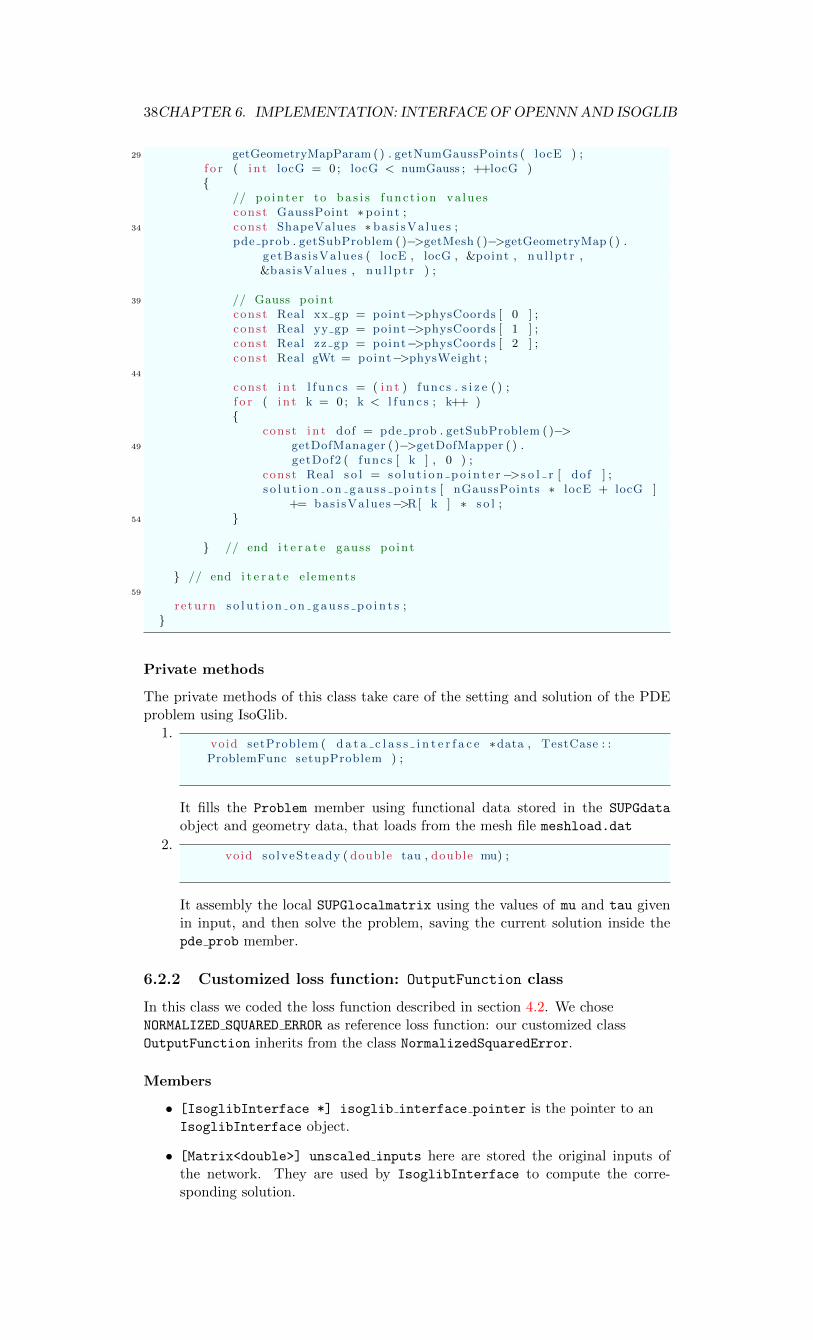
The main public method of this class[public] Vector <double> IsoglibInterface::calculate solution(

double tau, double mu) takes the input µ and the output τ of the network andreturns a vector containing the corresponding PDE solution, computed in the gausspoints of the mesh.

First, a scaling is computed for the value of tau predicted by the network, usingthe member tau scaling. After that, the private member solveSteady is calledand the solution of the problem is stored inside the pde prob member.

Through an IsoglibInterface object we are able to obtain the values neededto calculate our loss function, comparing the expected and the current solution.

To do this, we experimentally found out that perform a L2 discrete comparisonbetween the nodal values of the IsoGlib solution and exact solutions computed inthe same nodes, does not lead to a significant measurement of the performance ofthe approximation. Indeed it happened that the predicted solution was far awayfrom the exact one, but this type of loss indicated an optimal value.

To solve this problem we employ the most natural error measure in the fieldof PDEs: the L2 norm. We compute it through gaussian numerical integration, asdescribed in section 4.2.

For this reason, the second part of the function calculate solution changesthe nodes involved in the comparison, taking care of computing the value of thesolution in gauss points, using a loop on all the elements of the mesh.

[ pub l i c ] Vector <double> I s o g l i b I n t e r f a c e : : c a l c u l a t e s o l u t i o n ( doubletau , double mu)

double tau for EDP = tau ∗ t a u s c a l i n g ;

4 so lveSteady ( tau for EDP , mu) ;

// used to acce s s o l rs o l u t i o n c l a s s ∗ s o l u t i o n p o i n t e r = pde prob . getSubProblem ( ) >

ge tSo lu t i on ( ) ;9

// get e lements o f t h i s p roce s sconst i n t numMyElements = pde prob . getSubProblem ( ) >getMesh ( ) >

getNumMyElements ( ) ;

14 // s o l u t i o nVector<double> s o l u t i o n on gau s s p o i n t s ( numMyElements ∗

nGaussPoints , 0 ) ;

// compute value o f the s o l u t i o n on gauss po in t s f o r19 // each element

f o r ( i n t locE = 0 ; locE < numMyElements ; locE++ )

// elementconst Element &element = pde prob . getSubProblem ( ) >getMesh ( ) >

24 getGeometryMapParam ( ) . getLocalElement ( locE ) ;const v e c t i n t &funcs = element . f un c t i on s ;

// f o r each Gauss po in t si n t numGauss = pde prob . getSubProblem ( ) >getMesh ( ) >


29 getGeometryMapParam ( ) . getNumGaussPoints ( locE ) ;f o r ( i n t locG = 0 ; locG < numGauss ; ++locG )

// po in t e r to ba s i s f unc t i on va lue sconst GaussPoint ∗ point ;

34 const ShapeValues ∗ bas i sVa lue s ;pde prob . getSubProblem ( ) >getMesh ( ) >getGeometryMap ( ) .

ge tBas i sVa lues ( locE , locG , &point , nu l lp t r ,&bas i sValues , nu l l p t r ) ;

39 // Gauss po intconst Real xx gp = point >physCoords [ 0 ] ;const Real yy gp = point >physCoords [ 1 ] ;const Real zz gp = point >physCoords [ 2 ] ;const Real gWt = point >physWeight ;

44

const i n t l f u n c s = ( i n t ) funcs . s i z e ( ) ;f o r ( i n t k = 0 ; k < l f u n c s ; k++ )

const i n t dof = pde prob . getSubProblem ( ) >49 getDofManager ( ) >getDofMapper ( ) .

getDof2 ( funcs [ k ] , 0 ) ;const Real s o l = s o l u t i o n po i n t e r >s o l r [ dof ] ;s o l u t i o n on gau s s p o i n t s [ nGaussPoints ∗ locE + locG ]

+= bas i sValues >R[ k ] ∗ s o l ;54

// end i t e r a t e gauss po int

// end i t e r a t e e lements59

re turn s o l u t i o n on gau s s p o i n t s ;

Private methods

The private methods of this class take care of the setting and solution of the PDEproblem using IsoGlib.

1.void setProblem ( d a t a c l a s s i n t e r f a c e ∗data , TestCase : :ProblemFunc setupProblem ) ;

It fills the Problem member using functional data stored in the SUPGdata

object and geometry data, that loads from the mesh file meshload.dat

2.void so lveSteady ( double tau , double mu) ;

It assembly the local SUPGlocalmatrix using the values of mu and tau givenin input, and then solve the problem, saving the current solution inside thepde prob member.

6.2.2 Customized loss function: OutputFunction class

In this class we coded the loss function described in section 4.2. We choseNORMALIZED SQUARED ERROR as reference loss function: our customized classOutputFunction inherits from the class NormalizedSquaredError.

Members

• [IsoglibInterface *] isoglib interface pointer is the pointer to anIsoglibInterface object.

• [Matrix<double>] unscaled inputs here are stored the original inputs ofthe network. They are used by IsoglibInterface to compute the corre-sponding solution.


Private methods1.

[ p r i va t e ] Matrix<double> ca l cu l a t e PDE so lu t i on ( const Matrix<double>& tau va lues , const Vector<s i z e t > & ba t ch i nd i c e s )const ;

Calculates the solution of the PDE given the stabilization parameter pre-dicted by the neural network. Here batch indices indicates the indices ofthe instances contained in the current batch. They are used to select thecorresponding inputs.

Its implementation contains a loop over the current batch in which the solutionis computedVector<double> temp solution = isoglib interface pointer->

calculate solution(tau, mu); where mu is picked from the unscaled inputsand tau from the tau values, outputs of the network.

2.[ p r i va t e ]

Matrix<double> OutputFunction : : c a l c u l a t e l o s s d e r i v a t i v e ( constMatrix<double>& tau va lues , const Vector<s i z e t > &ba t ch i nd i c e s ) const

It computes the gradient of our loss function with respect to the stabilizationparameters. This method is involved in our customized backpropagation pro-cess, indeed the loss function is now composed by two function, and we haveto differentiate both of them.

First, the derivative of the normalized squared loss function with respect tothe PDE solution values is computed:Matrix<double> simple loss derivatives = PDE solutions - targets

Secondly, the derivative of the PDE solution with respect to the stabilizationparameter is computed.Matrix<double> PDE solutions derivatives =

calculate PDE solution derivative(tau values, batch indices)

This can be done thanks to the private membercalculate PDE solution derivative already described.

At the end, the implementation of this function contains a loop in which thecomposition of the two derivatives is computed, exploiting the subdivision ofthe dataset into batches.

3.[ p r i va t e ]Matrix<double> c a l c u l a t e PDE so l u t i on d e r i v a t i v e ( const Matrix<

double>& tau va lues , const Vector<s i z e t > & ba t ch i nd i c e s )const ;

This method calculates the derivative of the PDE solution with respect tothe stabilization parameter. Since the function that relates these two valuesinvolve a call to many IsoGlib functions, this derivative cannot be computeexactly, but it must be subject to an approximation. How we explained insection 4.2 we choose to approximate it using Numerical Differentiation.

In this method this approximation is obtained through two sequential call tothe function that computes the PDE solution:Vector<double> y = isoglib interface pointer->calculate solution(tau,

mu);

Vector<double> y forward =

isoglib interface pointer->calculate solution(tau + h, mu);

Vector<double> derivative = ( y forward - y ) / h;

Public methods that perform override

The following methods are directly involved in the training process and they overridethe version implemented inside the parent class NormalizedSquaredError. We will


describe them focusing on the differences with the description given in section 5.2.6.The idea is, given the stabilization parameter as output of the network, obtainthe corresponding PDE solution and then compare it with the target, using the”standard” normalized squared loss function .

1.[ pub l i c ] v i r t u a l double OutputFunction : : c a l c u l a t e t r a i n i n g e r r o r ( )

ov e r r i d e

In this method, the calculate the loss for the training dataset, we have addedthe call to the function that, given the output of the network, calculate thecorresponind PDE solution.

Matrix<double> PDE solutions = ca l cu l a t e PDE so lu t i on s ( outputs ,t r a i n i n g ba t ch e s [ s t a t i c c a s t <unsigned>( i ) ] ) ;

At this point, the normalized squared loss function is called to compare thissolution to the given targets.const double batch error =

PDE solutions.calculate sum squared error(targets);

2. The procedure just described is reapeated in other two overridden functions[public] double OutputFunction::calculate selection error() const

[public] double OutputFunction::calculate training error

(const Vector<double>& parameters) const

whose scope is the same, but are used in different points of the training pro-cess.

3.[ pub l i c ]Vector<double> OutputFunction : : c a l c u l a t e t r a i n i n g e r r o r g r a d i e n t ( )

This function is crucial in the backpropagation process and its parent classversion has been deeply described in section 5.2.8.

This call makes the difference with respect to the NormalizedSquaredError

version:const Matrix<double> output gradient =

calculate loss derivative

(first order forward propagation.layers activations[layers number-1],

training batches[static cast<unsigned>(i)]);

Indeed we have substituted the call to calculate output gradient, that cal-culates the derivative of the loss function with respect to the output of the net-work, with the call to the new private member calculate loss derivative.

This function still calculates the gradient of the loss function with respectto the outputs(stabilization parameters), but since we have enriched our lossfunction,this is now computed in a different way, as previously described.

Implementation of the private methods1.

/// \param tau va lue s S t a b i l i z a t i o n parameters [c u r r e n t b a t c h s i z e x 1 ]

/// \param ba t ch i nd i c e s Indeces o f the cur rent batch ,used to s e l e c t the inputs [ c u r r e n t b a t c h s i z e ]

3 /// \ re turn PDE s o l u t i o n s [c u r r e n t b a t c h s i z e x n Dof ]

Matrix<double> OutputFunction : : c a l cu l a t e PDE so lu t i on ( constMatrix<double>& tau va lues , const Vector<s i z e t > &ba t ch i nd i c e s ) const

unsigned elements number = i s o g l i b i n t e r f a c e p o i n t e r >

8 get nElems ( ) ;


unsigned gauss points number = i s o g l i b i n t e r f a c e p o i n t e r >get nGaussPoints ( ) ;

unsigned cu r r e n t b a t c h s i z e = ba t ch i nd i c e s . s i z e ( ) ;Matrix<double> s o l u t i o n s ( cu r r en t ba t ch s i z e ,

13 elements number∗ gauss points number ) ;

f o r ( s i z e t i = 0 ; i < c u r r e n t b a t c h s i z e ; i++)

Real mu = unsca l ed input s ( ba t ch i nd i c e s [ i ] , 0) ;18 Real tau = tau va lue s ( i , 0) ;

Vector<double> t emp so lut ion =i s o g l i b i n t e r f a c e p o i n t e r >c a l c u l a t e s o l u t i o n ( tau , mu) ;

23 s o l u t i o n s . s e t row ( i , t emp so lut ion ) ;

re turn s o l u t i o n s ;

2./// \param tau va lue s S t a b i l i z a t i o n parameters [

c u r r e n t b a t c h s i z e x 1 ]/// \param ba t ch i nd i c e s Indeces o f the cur rent batch ,

used to s e l e c t the inputs [ c u r r e n t b a t c h s i z e ]3 /// \ re turn Der iva t ive o f the l o s s func t i on

wrt the s t a b i l i z a t i o n parameter [ c u r r e n t b a t c h s i z e x 1 ]

Matrix<double> OutputFunction : : c a l c u l a t e l o s s d e r i v a t i v e ( constMatrix<double>& tau va lues , const Vector<s i z e t > &ba t ch i nd i c e s ) const

unsigned cu r r e n t b a t c h s i z e = ba t ch i nd i c e s . s i z e ( ) ;

8

Matrix<double> PDE solutions =ca l cu l a t e PDE so lu t i on ( tau va lues , b a t ch i nd i c e s ) ;

const Matrix<double> t a r g e t s =da ta s e t po i n t e r >g e t t a r g e t s ( ba t ch i nd i c e s ) ;

13

Matrix<double> s imp l e l o s s d e r i v a t i v e s =PDE solutions ´ t a r g e t s ;

Matrix<double> PDE so lu t i on s de r i va t i v e s =ca l cu l a t e PDE so l u t i on d e r i v a t i v e ( tau va lues ,

18 ba t ch i nd i c e s ) ;

Matrix<double>c ompo s ed l o s s d e r i v a t i v e s ( cu r r en t ba t ch s i z e , 1) ;

23 f o r ( i n t i = 0 ; i < c u r r e n t b a t c h s i z e ; i++)

c ompo s ed l o s s d e r i v a t i v e s ( i , 0) =s imp l e l o s s d e r i v a t i v e s . get row ( i ) .dot ( PDE so lu t i on s de r i va t i v e s . get row ( i ) ) ;

28

re turn compo s ed l o s s d e r i v a t i v e s ;

3./// \param tau va lue s S t a b i l i z a t i o n parameters [

c u r r e n t b a t c h s i z e x 1 ]/// \ re turn Der iva t ive o f the PDE so l u t i o n

wrt the s t a b i l i z a t i o n parameter [ c u r r e n t b a t c h s i z e x n Dof ]Matrix<double> OutputFunction : : c a l c u l a t e PDE so l u t i on d e r i v a t i v e

( const Matrix<double>& tau va lues , const Vector<s i z e t > &ba t ch i nd i c e s ) const

4 unsigned elements number = i s o g l i b i n t e r f a c e p o i n t e r >get nElems ( ) ;unsigned gauss points number = i s o g l i b i n t e r f a c e p o i n t e r >get nGaussPoints ( ) ;


9 unsigned cu r r e n t b a t c h s i z e = ba t ch i nd i c e s . s i z e ( ) ;Matrix<double> s o l u t i o n s d e r i v a t i v e s ( cu r r en t ba t ch s i z e ,

elements number∗ gauss points number ) ;

f o r ( i n t i = 0 ; i < c u r r e n t b a t c h s i z e ; i++)14

double mu = unsca l ed input s ( ba t ch i nd i c e s [ i ] , 0) ;double tau = tau va lue s ( i , 0) ;

double h = 0 . 1 ;19 Vector<double> y = i s o g l i b i n t e r f a c e p o i n t e r >

c a l c u l a t e s o l u t i o n ( tau , mu) ;Vector<double> y forward = i s o g l i b i n t e r f a c e p o i n t e r >

c a l c u l a t e s o l u t i o n ( tau + h , mu) ;Vector<double> d e r i v a t i v e = ( y forward ´ y ) / h ;

24

s o l u t i o n s d e r i v a t i v e s . s e t row ( i , d e r i v a t i v e ) ;

re turn s o l u t i o n s d e r i v a t i v e s ;29

6.3 SUPG example in OpenNN

In this customized example (OpenNN/examples/SUPG) is where we actually imple-mented the construction, training and testing of our neural network. Here we ex-ploited all the described features of OpenNNN library and all the new classes wewrote, to customize our network and carry out our idea.

6.3.1 Data of the problem

In the first part, the number of the Test Problem is settled, according with theref number, that indicates the mesh refinement. These information are enough toidentify the folders where the data file meshload.dat and the dataset SUPG.txt canbe found.

1 unsigned test number = 1 ;unsigned ref number = 3 ;s t r i n g dataset name = ”data/Test ”+ t o s t r i n g ( test number ) + ”/ r e f ” +

t o s t r i n g ( ref number )+ ”/SUPG. txt ” ;s t r i n g mesh load fo lde r = ”data/Test ” + t o s t r i n g ( test number ) + ”/ r e f ”

+ t o s t r i n g ( ref number ) ;

Then, loading the data from this txt file, a DataSet object is created,and thenumber of inputs and targets for the network are setted.

6.3.2 Training

The NeuralNetwork and TrainingStrategy objects are created, as described insection 5.2.4 and 5.2.5. In particular, for our network, we customized in this wayour TrainingStrategy object:

• We set GRADIENT DESCENT as algorithm used for the trainingtraining strategy.set training method( "GRADIENT DESCENT")

• We set the loss method such that the training prcoess uses our customizedloss function OutputFunction. The creation of the OutputFunction pointeris made giving in input the name of the folder where the mesh data file is storedand the data class (SUPGdata[numberoftest]) created accordingly to the testnumber. Some information about the PDE problem (gauss points number, el-ements number, dofs number) are then setted in the isoglibinterface pointer

stored in the output function pointer.

6.3. SUPG EXAMPLE IN OPENNN 43

1 SUPGdata1 data1 ;SUPGdata2 data2 ;SUPGdataBase∗ data po in t e r ;i f ( test number == 1 )

da ta po in t e r = &data1 ;6 e l s e i f ( test number == 2 )

da ta po in t e r = &data2 ;

OutputFunction ∗ ou tpu t f unc t i on po i n t e r = new OutputFunction (mesh load fo lder , da ta po in t e r )

11 t r a i n i n g s t r a t e g y . s e t l o s s i n d e x p o i n t e r ( ou tpu t f unc t i on po i n t e r )

To perform training, once all the data have been setted, the methodperform training() is calledconst TrainingStrategy::Results training strategy results =

training strategy.perform training() and all the crucial results are savedin a TrainingStrategy::Results object.

At the end of the training phase, we save the history of the training andvalidation errors, that we use (see 7) to analyze our numerical tests.

Vector<double> l o s s h i s t o r y =t r a i n i n g s t r a t e g y r e s u l t s .g r a d i e n t d e s c e n t r e s u l t s p o i n t e r >l o s s h i s t o r y ;

Vector<double> s e l e c t i o n h i s t o r y=t r a i n i n g s t r a t e g y r e s u l t s .g r a d i e n t d e s c e n t r e s u l t s p o i n t e r >s e l e c t i o n e r r o r h i s t o r y ;

s i z e t l o s s s i z e= l o s s h i s t o r y . s i z e ( ) ;

6.3.3 Testing

For the testing phase of our network, we used an object of type TestingAnalysis.In particular, through the function calculate target outputs is possible tocompute the outputs of the network corresponding to the testing inputs of thedataset, instances that have never been used in the training phase, so unknownfor the Neural Network.

1 Test ingAna lys i s t e s t i n g a n a l y s i s (&neural network , &da ta s e t ) ;

Vector<Matrix<double>> r e s u l t s = t e s t i n g a n a l y s i s .c a l c u l a t e t a r g e t o u t pu t s ( ) ;

To visualize the results, we scale the inputs using the inputs statistics

data, and the stabilization paremters (outputs) using the scaling coefficentsstored in the IsoglibI nterface pointer.

Chapter 7

Numerical Tests

We now present some numerical results obtained using Isogeometric elements of thefirst order to solve a two-dimensional advection-diffusion problem. For the testingphase of our network we chose a problem for which the value of the exact solutionis known. This choice simplified the creation of the dataset, since the targets canbe obtained with a simple function evaluation in the gauss nodes. However, thishypothesis can be removed: solving once on a very fine mesh is then needed (seesection 4.1).

The problem belongs to the family of PDEs 2.1, with the restrictions of µ andb constant in space. We fixed the domain Ω, the forcing term f , the mesh size hand the advection coefficient b, leaving only µ as variable. Its influence on the bestvalue of the stabilization parameter is the object of our interest.

The problem is defined given:

• Ω “ p0, 1q2

• b “ p1, 1q

• fpxq “ sinp2πxqrµp2` 4π2py ´ y2qq ` p1´ 2yqs2π cosp2πxqp2` 4π2py ´ y2qq

• g “ 0

so that the exact solution (represented in figure 7.1) is given by:

uex “ sinp2πxqpy ´ y2q

As we can see in Figure 7.2, the numerical solution obtained for µ “ 10´4

presents numerical oscillations.

Figure 7.1: Exact solution in the case µ “ 10´4

45

46 CHAPTER 7. NUMERICAL TESTS

Figure 7.2: Numerical oscillations in the case µ “ 10´4

7.1 Training of the network

For this Test Case we created the SUPGdata1 class where we stored all the termsdefining the PDE problem (see section 6.1.1 for more details). We tested our networkon different datasets, generated with a Matlab script. The script takes care ofevaluating the exact solution in the correct points (the gauss nodes), respecting theorder in which pointwise comparison is performed inside OpenNN during the trainingof the ANN.

The first problem we faced was the choice of the training set. We started con-sidering data sets with about 20 instances without obtaining satisfactory results, aswe can see in Figure 7.3 the magnitude of τ increases as the one of µ do the same,behaviour that is not aligned with theory.

Figure 7.3: Predicted τ values after training with a 20instances dataset

Then we tried distributing logarithmically the values of the input but predictionswere even worse. When we started taking big data sets the results became betterand better as the training set grows, suggesting that the number of instances is themain factor influencing the efficiency of the learning. So we decided to train ourANN with data sets of 200-300 instances.

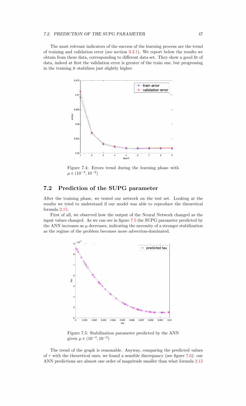
7.2. PREDICTION OF THE SUPG PARAMETER 47

The most relevant indicators of the success of the learning process are the trendof training and validation error (see section 3.3.1). We report below the results weobtain from these data, corresponding to different data set. They show a good fit ofdata, indeed at first the validation error is greater of the train one, but progressingin the training it stabilizes just slightly higher.

Figure 7.4: Errors trend during the learning phase withµ P p10´4, 10´2q

7.2 Prediction of the SUPG parameter

After the training phase, we tested our network on the test set. Looking at theresults we tried to understand if our model was able to reproduce the theoreticalformula 2.15.

First of all, we observed how the output of the Neural Network changed as theinput values changed. As we can see in figure 7.5 the SUPG parameter predicted bythe ANN increases as µ decreases, indicating the necessity of a stronger stabilizationas the regime of the problem becomes more advection-dominated.

Figure 7.5: Stabilization parameter predicted by the ANNgiven µ P p10´4, 10´2q

The trend of the graph is reasonable. Anyway, comparing the predicted valuesof τ with the theoretical ones, we found a sensible discrepancy (see figure 7.6): ourANN predictions are almost one order of magnitude smaller than what formula 2.15


states. To understand whether our code was performing correctly we needed tobetter analyze the norm we have chosen to measure the error during the training.

Figure 7.6: Predicted vs theoretical τ for µ P p10´4, 10´2q

7.3 Analysis of the results

First of all, we have verified that the numerical solutions computed using the stabi-lization parameter predicted by the network does not present numerical oscillations.In figure 7.7 we can see the stabilized (by the network) numerical solution, corre-sponding to µ “ 10´4. Analyzing figure 7.6, we can deduce that the theoreticalestimate is pessimist: it forecast a stabilization parameter that is greater than theone needed to eliminate oscillations.

Figure 7.7: Stabilized solution in the case µ “ 10´4

Since the aim of our Neural Network is to minimize the L2 norm between thestabilized and exact solution, we asked ourselves if the value of the parameter ob-tained with this procedure is coherent with the theoretical one. A priori, we donot have any guarantee that the best SUPG parameter from the point of view, forexample, of the respect of the Maximum Principle (see section 2.2.1) is the samethat minimizes the L2 error between exact and numerical solution. We used IsoGlibto solve the PDE problem with a fixed µ modifying the magnitude of τ in order tofind the value of the stabilization parameter that minimizes the L2 error. Exploiting

7.3. ANALYSIS OF THE RESULTS 49

the classes put in charge of errors computation already implemented inside IsoGlib,we found that an optimal SUPG parameter exists (See figure 7.8) in all the casestested, but does not coincide with the theoretical one.

Figure 7.8: The L2 error for µ “ 5 ¨ 10´4 computed fordifferent values of τ using IsoGlib. The function has a welldefined minimum, the corresponding value of τ is what wedefine optimal stabilization parameter.

Fixing different values of µ and looking for the minimum of the L2 error withrespect to τ we obtained the results shown in table 7.3 :

µ theoretical τ L2-optimal τ

1 ¨ 10´5 4.42 ¨ 10´2 9.56 ¨ 10´3

5 ¨ 10´5 4.42 ¨ 10´2 9.52 ¨ 10´3

1 ¨ 10´4 4.41 ¨ 10´2 9.46 ¨ 10´3

5 ¨ 10´4 4.39 ¨ 10´2 9.00 ¨ 10´3

1 ¨ 10´3 4.37 ¨ 10´2 8.43 ¨ 10´3

5 ¨ 10´3 4.17 ¨ 10´2 4.02 ¨ 10´3

Table 7.1: Comparison between values of τ predicted by 2.15 and by the ANN

As we can see the two values does not coincide. Since for the training of the ANNwe used an analogous metric to the one adopted by IsoGlib, we can expect our pre-diction coming from the (well working) ANN to be closer to the value we measuredexperimentally.

Comparing the predictions made by the ANN on the test set with the L2-optimalvalues just computed we can see the perfect agreement of the two.

In figure 7.10 we can see the optimal prediction after the complete training of theNeural Network. Besides, in figure 7.9 we report the τ predictions after a trainingwith just 2 epochs. It is clear how the forecasting of the value of τ gets better goingahead with the training.

This result suggests that the Neural Network is actually performing well, learn-ing from the data set how to minimize the L2 error between exact and numericalsolution. The discrepancy from the theoretical expectations could then be ascribedto the choice of the norm adopted in the loss function.


Figure 7.9: L2-optimal and predicted τ values, trainingwith 2 epochs

Figure 7.10: L2-optimal and predicted τ values, trainingwith 9 epochs

7.4 L2 error trend in a different PDE

Once we understood that the ANN worked correctly, we changed the test problem.We fixed:

• Ω “ p0, 1q2

• b “ p1, 1q

• g “ 0

and fpxq such that the exact solution is:

uex “1

10e4ypy ´ 1qpx´ 1qx

We expected, as formula 2.15 suggests, that the best SUPG parameter depends onlyon the value of the diffusion coefficient (once the other parameters have been fixed).Performing the same kind of analysis described in the previous section, we foundthat the best values for τ (with respect to L2 norm) corresponding to the same valueof µ were now different. In figure (7.11) this difference can be seen evidently.

7.4. L2 ERROR TREND IN A DIFFERENT PDE 51

Figure 7.11: L2-optimal τ for two different problems

As a consequence of this behavior of the network, any effort of approximating therelation between µ and τ have to be connected to the problem object of analysis.In practice: at the present state, our ANN can not be used, since training anddeployment must happen on the same PDE. Future developments will be discussedin the conclusions.

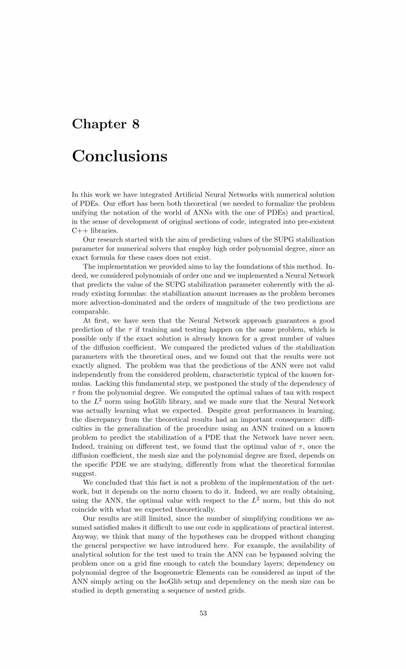
Chapter 8

Conclusions

In this work we have integrated Artificial Neural Networks with numerical solutionof PDEs. Our effort has been both theoretical (we needed to formalize the problemunifying the notation of the world of ANNs with the one of PDEs) and practical,in the sense of development of original sections of code, integrated into pre-existentC++ libraries.

Our research started with the aim of predicting values of the SUPG stabilizationparameter for numerical solvers that employ high order polynomial degree, since anexact formula for these cases does not exist.

The implementation we provided aims to lay the foundations of this method. In-deed, we considered polynomials of order one and we implemented a Neural Networkthat predicts the value of the SUPG stabilization parameter coherently with the al-ready existing formulas: the stabilization amount increases as the problem becomesmore advection-dominated and the orders of magnitude of the two predictions arecomparable.

At first, we have seen that the Neural Network approach guarantees a goodprediction of the τ if training and testing happen on the same problem, which ispossible only if the exact solution is already known for a great number of valuesof the diffusion coefficient. We compared the predicted values of the stabilizationparameters with the theoretical ones, and we found out that the results were notexactly aligned. The problem was that the predictions of the ANN were not validindependently from the considered problem, characteristic typical of the known for-mulas. Lacking this fundamental step, we postponed the study of the dependency ofτ from the polynomial degree. We computed the optimal values of tau with respectto the L2 norm using IsoGlib library, and we made sure that the Neural Networkwas actually learning what we expected. Despite great performances in learning,the discrepancy from the theoretical results had an important consequence: diffi-culties in the generalization of the procedure using an ANN trained on a knownproblem to predict the stabilization of a PDE that the Network have never seen.Indeed, training on different test, we found that the optimal value of τ , once thediffusion coefficient, the mesh size and the polynomial degree are fixed, depends onthe specific PDE we are studying, differently from what the theoretical formulassuggest.

We concluded that this fact is not a problem of the implementation of the net-work, but it depends on the norm chosen to do it. Indeed, we are really obtaining,using the ANN, the optimal value with respect to the L2 norm, but this do notcoincide with what we expected theoretically.

Our results are still limited, since the number of simplifying conditions we as-sumed satisfied makes it difficult to use our code in applications of practical interest.Anyway, we think that many of the hypotheses can be dropped without changingthe general perspective we have introduced here. For example, the availability ofanalytical solution for the test used to train the ANN can be bypassed solving theproblem once on a grid fine enough to catch the boundary layers; dependency onpolynomial degree of the Isogeometric Elements can be considered as input of theANN simply acting on the IsoGlib setup and dependency on the mesh size can bestudied in depth generating a sequence of nested grids.

53

Bibliography

[HB82] Hughes, Thomas J. R.; Brooks, A. N. (1982), A theoretical framework forPetrov-Galerkin methods with discontinuous weighting functions: application tothe streamline-upwind procedure

[Q17] Quarteroni, Alfio (2017), Numerical Models for Differential Problems,Springer International; 16, pp. 61-114, 267-292, 315-362

[CHB09] Cottrell,J.Austin; Hughes, Thomas J. R; Bazilevs, Yuri (2009) Isogeomet-ric Analysis, John Wiley Sons, Ltd, pp. 19-108.

[AQ11] Quarteroni, Alfio; Antonietti, Paola F.A. (2013), Numerical perfor-mance of discontinuous and stabilized continuous Galerkin methods for convec-tion–diffusion problems, Proceedings of the International Conference on Numer-ical Methods for Hyperbolic Equations: Theory and Applications pp. 75-85

[HSF18] Hughes, Thomas J. R.; Scovazzi, Guglielmo; Franca, Leopoldo P. (2018),Multiscale and Stabilized Methods, Encyclopedia of Computational MechanicsSecond Edition, pp. 1-64

[HEV07] Houzeaux, Guillaume; Eguzkitza Beatriz; Vazquez Mariano (2007), AVariational Multiscale Model Based on the Analytical Solution of the Approx-imate Subgrid Scale Equation, Preprint submitted to Comp. Meth. Appl. Mech.Eng., 2007

[C97] Codina, Ramon (1997), Comparison of some finite element methods for solv-ing the diffusion-convection-reaction equation, Computer Methods in AppliedMechanics and Engineering, 156, pp. 185-210

[C89] Cybenko, George (1989), Approximation by superpositions of a sigmoidalfunction, G. Math. Control Signal Systems 2, p. 303

[RDQ19] Regazzoni, Francesco; Dede, Luca; Quarteroni, Alfio (2019), Machinelearning for fast and reliable solution of time-dependent differential equations,Journal of Computational Physics num. 397

[OpenNN] OpenNN C++ library Copyright: Artificial Intelligence Techniques SL.Github page of OpenNNOpenNN website

[R96] Rojas, Raul (1996), Neural Networks - A Systematic Introduction, SpringerInternational, pp. 55-99, 151-184

[NUR] NURBS octave/MATLAB package Nurbs package webpage

55

https://github.com/Artelnics/OpenNN

http://www.opennn.net

http://octave.sourceforge.io/nurbs

machine learning for numerical stabilization of advection

Documents