Machine Learning for Multi-stepAhead Forecasting of Volatility

ProxiesJacopo De Stefani, Ir. - jdestefa@ulb.ac.beProf. Gianluca Bontempi - gbonte@ulb.ac.be

Olivier Caelen, PhD - olivier.caelen@worldline.comDalila Hattab, PhD - dalila.hattab@equensworldline.com

MIDAS 2017 - ECML-PKDDHotel Aleksandar Palace, Skopje, FYROM

Monday 18th September, 2017

Problem overview

25

30

35

40

45

First series CAC40 [2012−01−02/2013−11−04]

Last 47.255

Volume (100,000s):

345,721

0

10

20

30

40

50

Moving Average Convergence Divergence (12,26,9):

MACD: 1.335

Signal: 1.258

−3

−2

−1

0

1

2

3

Jan 022012

Mar 012012

May 022012

Jul 022012

Sep 032012

Nov 012012

Jan 022013

Mar 012013

May 022013

Jul 012013

Sep 022013

Nov 012013

2/32

What is volatility?

DefinitionVolatility is a statistical measure of the dispersion of returns for agiven security or market index.

0 20 40 60 80 100

−1

−0.5

0

0.5

1High volatility Low volatility

t [days]

r t

3/32

A closer look on data - Volatility proxies

0 0.2 0.4 0.6 0.8 1 1.2 1.4

9.8

10

10.2

P o0

P h0

P l0

P c0

P o1

P h1

P l1

P c1

Pre-opening

1− f f 1− f

Calendar Day 0 Calendar Day 1

t [days]

Pt

Volatility proxy

P otP htP ltP ct

σPt

4/32

Models for volatility

Volatility models

Pastvolatility

Average-based

HA

MAES

EWMA

STES

SimpleRegression

SR-AR

SR-TAR

SR-ARMA

RandomWalk

ARCH

Symmetric

ARCH (q)

GARCH(p,q)

Asymmetric

EGARCH(p,q)

GJR-GARCH(p,q)

QGARCH(p,q)

ST-GARCH(p,q)

RS-GARCH(p,q)Extended

Component-GARCH(p,q)

RGARCH(p,q)

MachineLearningUnivariateNN

k-NN

SVR

Multivariate

5/32

Models for volatility

Volatility models

Pastvolatility

Average-based

HA

MAES

EWMA

STES

SimpleRegression

SR-AR

SR-TAR

SR-ARMA

RandomWalk

ARCH

Symmetric

ARCH (q)

GARCH(p,q)

Asymmetric

EGARCH(p,q)

GJR-GARCH(p,q)

QGARCH(p,q)

ST-GARCH(p,q)

RS-GARCH(p,q)Extended

Component-GARCH(p,q)

RGARCH(p,q)

MachineLearningUnivariateNN

k-NN

SVR

Multivariate

5/32

Models for volatility

Volatility models

Pastvolatility

Average-based

HA

MAES

EWMA

STES

SimpleRegression

SR-AR

SR-TAR

SR-ARMA

RandomWalk

ARCH

Symmetric

ARCH (q)

GARCH(p,q)

Asymmetric

EGARCH(p,q)

GJR-GARCH(p,q)

QGARCH(p,q)

ST-GARCH(p,q)

RS-GARCH(p,q)Extended

Component-GARCH(p,q)

RGARCH(p,q)

MachineLearningUnivariateNN

k-NN

SVR

Multivariate

Established Research

5/32

Models for volatility

Volatility models

Pastvolatility

Average-based

HA

MAES

EWMA

STES

SimpleRegression

SR-AR

SR-TAR

SR-ARMA

RandomWalk

ARCH

Symmetric

ARCH (q)

GARCH(p,q)

Asymmetric

EGARCH(p,q)

GJR-GARCH(p,q)

QGARCH(p,q)

ST-GARCH(p,q)

RS-GARCH(p,q)Extended

Component-GARCH(p,q)

RGARCH(p,q)

MachineLearningUnivariateNN

k-NN

SVR

Multivariate

Established Research

Future Research

5/32

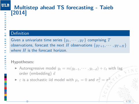
Multistep ahead TS forecasting - Taieb[2014]

DefinitionGiven a univariate time series {y1, · · · , yT } comprising Tobservations, forecast the next H observations {yT+1, · · · , yT+H}where H is the forecast horizon.

Hypotheses:I Autoregressive model yt = m(yt−1, · · · , yt−d) + εt with lag

order (embedding) dI ε is a stochastic iid model with µε = 0 and σ2

ε = σ2

6/32

Multistep ahead forecasting for volatilityState-of-the-art

NAR

m(σP)

· · · σPt−1][σPt−d

· · ·[σPt σPt+H ]

1 Input1 Output

Proposed modelNARX

m(σP, σX)

· · ·· · ·

σXt−1]σPt−1]

[σXt−d[σPt−d

· · ·[σPt σPt+H ]

2 inputs1 output

Future work

m(σP, · · · , σXM)

· · ·· · ·· · ·

σXMt−1 ]· · · ]σPt−1]

[σXMt−d

[· · ·[σPt−d

· · ·· · ·· · ·

[σPt[· · ·

[σXMt

σPt+H ]· · · ]σXMt+H ]

M + 1 inputsM + 1 outputs

7/32

Multistep ahead forecasting for volatilityState-of-the-art

NAR

m(σP)

· · · σPt−1][σPt−d

· · ·[σPt σPt+H ]

1 Input1 Output

Proposed modelNARX

m(σP, σX)

· · ·· · ·

σXt−1]σPt−1]

[σXt−d[σPt−d

· · ·[σPt σPt+H ]

2 inputs1 output

Future work

m(σP, · · · , σXM)

· · ·· · ·· · ·

σXMt−1 ]· · · ]σPt−1]

[σXMt−d

[· · ·[σPt−d

· · ·· · ·· · ·

[σPt[· · ·

[σXMt

σPt+H ]· · · ]σXMt+H ]

M + 1 inputsM + 1 outputs

7/32

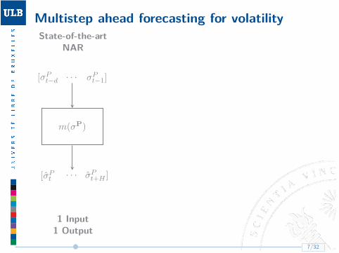
Multistep ahead forecasting for volatilityState-of-the-art

NAR

m(σP)

· · · σPt−1][σPt−d

· · ·[σPt σPt+H ]

1 Input1 Output

Proposed modelNARX

m(σP, σX)

· · ·· · ·

σXt−1]σPt−1]

[σXt−d[σPt−d

· · ·[σPt σPt+H ]

2 inputs1 output

Future work

m(σP, · · · , σXM)

· · ·· · ·· · ·

σXMt−1 ]· · · ]σPt−1]

[σXMt−d

[· · ·[σPt−d

· · ·· · ·· · ·

[σPt[· · ·

[σXMt

σPt+H ]· · · ]σXMt+H ]

M + 1 inputsM + 1 outputs

7/32

Multistep ahead forecasting for volatility

Direct method

I A single model fh for each horizon h.I Forecast at h step is made using hth model.I Dataset examples (d = 3, h = 3):

Direct NAR

x yσP

3 σP2 σP

1 σP5

σP4 σP

3 σP2 σP

6

... ... ... ...

σPT −5 σP

T −6 σPT −7 σP

T −2

Direct NARX

x yσP

3 σP2 σP

1 σX3 σX

2 σX1 σP

5

σP4 σP

3 σP2 σX

4 σX3 σX

2 σP6

... ... ... ... ... ... ...

σPT −5 σP

T −6 σPT −7 σX

T −5 σXT −6 σX

T −7 σPT −2

8/32

Experimental setup

m(σP, σX)

· · ·· · ·

σXt−1]σPt−1]

[σXt−d[σPt−d

· · ·[σPt σPt+H ]

2 TS Input1 TS Output

Data: Volatility proxies σX , σP from CAC40:I Price based

I σi family - Garman and Klass[1980]

I Return basedI GARCH (1,1) model - Hansen

and Lunde [2005]I Sample standard deviation

Models:I Feedforward Neural Networks

(NAR,NARX)I k-Nearest Neighbours (NAR,NARX)I Support Vector Regression (NAR,NARX)I Naive (w/o σX)I GARCH(1,1) (w/o σX)I Average (w/o σX)

9/32

Correlation meta-analysis (cf. Field [2001])

?

?

?

?

?

?

?

?

?

?

?

?

?

−1

−0.8

−0.6

−0.4

−0.2

0

0.2

0.4

0.6

0.8

1V

olu

me

σ 1 σ 6 σ 4 σ 5 σ 2 σ 3 r t σ 0 σ SD

25

0

σ SD

10

0

σ SD

50

σ G

Volume

σ1

σ6

σ4

σ5

σ2

σ3

rt

σ0

σSD

250

σSD

100

σSD

50

σG

I 40 time series(CAC40)

I Time range:05-01-2009 to22-10-2014

I 1489 OHLCsamples perTS

I Hierarchicalclusteringusing Ward Jr[1963]

I Allcorrelationsarestatisticallysignificant

10/32

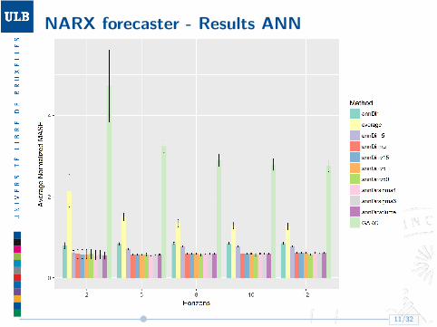
NARX forecaster - Results ANN

11/32

NARX forecaster - Results ANN

12/32

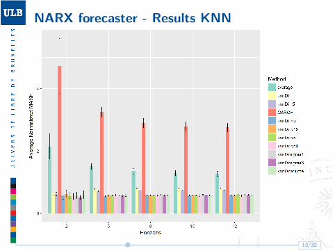
NARX forecaster - Results KNN

13/32

NARX forecaster - Results KNN

14/32

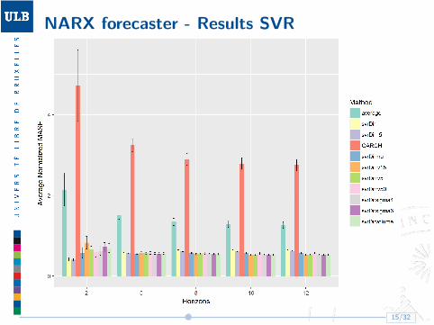
NARX forecaster - Results SVR

15/32

NARX forecaster - Results SVR

16/32

Conclusions

I Correlation clustering among proxies belonging to the samefamily, i.e. σit and σ

SD,nt .

I All ML methods outperform the reference GARCH method,both in the single input and the multiple input configuration.

I Only the addition of an external regressor, and for h > 8 bringa statistically significant improvement (paired t-test,pv=0.05).

I No model appear to clearly outperform all the others on everyhorizons, but generally SVR performs better than ANN andk-NN.

17/32

Thank you for your attention! Any questions/comments?jacopo.de.stefani@ulb.ac.be

Find the paper at:

18/32

Bibliography I

References

Tim Bollerslev. Generalized autoregressive conditionalheteroskedasticity. Journal of econometrics, 31(3):307–327,1986.

Andy P Field. Meta-analysis of correlation coefficients: a montecarlo comparison of fixed-and random-effects methods.Psychological methods, 6(2):161, 2001.

Mark B Garman and Michael J Klass. On the estimation ofsecurity price volatilities from historical data. Journal ofbusiness, pages 67–78, 1980.

19/32

Bibliography II

Peter R Hansen and Asger Lunde. A forecast comparison ofvolatility models: does anything beat a garch (1, 1)? Journal ofapplied econometrics, 20(7):873–889, 2005.

Rob J Hyndman and Anne B Koehler. Another look at measures offorecast accuracy. International journal of forecasting, 22(4):679–688, 2006.

Souhaib Ben Taieb. Machine learning strategies formulti-step-ahead time series forecasting. PhD thesis, Ph. D.Thesis, 2014.

Joe H Ward Jr. Hierarchical grouping to optimize an objectivefunction. Journal of the American statistical association, 58(301):236–244, 1963.

20/32

Appendix

21/32

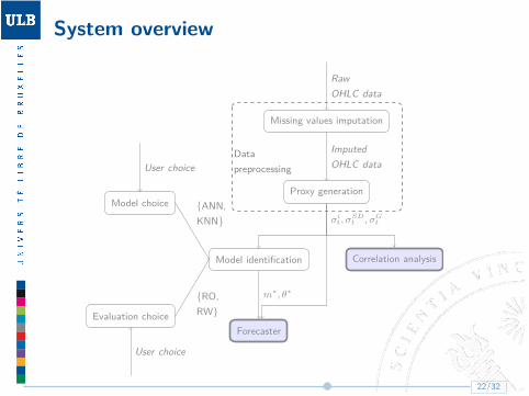
System overview

Missing values imputation

Proxy generation

Correlation analysisModel identification

Model choice

Evaluation choiceForecaster

RawOHLC data

ImputedOHLC data

σit, σ

SDt , σG

t

{ANN,KNN}

{RO,RW}

m∗, θ∗

User choice

User choice

Datapreprocessing

22/32

System overview

Missing values imputation

Proxy generation

Correlation analysisModel identification

Model choice

Evaluation choiceForecaster

RawOHLC data

ImputedOHLC data

σit, σ

SDt , σG

t

{ANN,KNN}

{RO,RW}

m∗, θ∗

User choice

User choice

Datapreprocessing

22/32

System overview

Missing values imputation

Proxy generation

Correlation analysisModel identification

Model choice

Evaluation choiceForecaster

RawOHLC data

ImputedOHLC data

σit, σ

SDt , σG

t

{ANN,KNN}

{RO,RW}

m∗, θ∗

User choice

User choice

Datapreprocessing

22/32

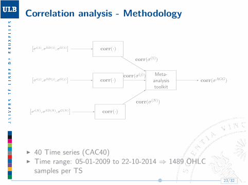
Correlation analysis - Methodology

[σi(1), σSD(1), σG(1)

]

[σi(j), σSD(j), σG(j)

]

[σi(N), σSD(N), σG(N)

]

corr(·)

corr(·)

corr(·)

Meta-analysistoolkit

corr(σAGG)

corr(σ(1))

corr(σ(j))

corr(σ(N))

I 40 Time series (CAC40)I Time range: 05-01-2009 to 22-10-2014 ⇒ 1489 OHLC

samples per TS23/32

NARX forecaster - Methodology

σJpOriginalDGP

Disturbances

d

Modelm∗(θ∗, σJ

p , σXp )

Structuralidentification

Parametricidentification

{ANN,KNN}{RO, RW}

σXp

eσJf

σJf

m∗(·, σJp , σXp ) θ∗

Model identification

24/32

Volatility proxies (1) - Garman and Klass [1980]I Closing prices

σ0(t) =

[ln

(P

(c)t+1

P(c)t

)]2

= r2t (1)

I Opening/Closing prices

σ1(t) = 12f ·

[ln

(P

(o)t+1

P(c)t

)]2

︸ ︷︷ ︸Nightly volatility

+ 12(1− f) ·

[ln(P

(c)t

P(o)t

)]2

︸ ︷︷ ︸Intraday volatility

(2)

I OHLC prices

σ2(t) = 12 ln 4 ·

[ln(P

(h)t

P(l)t

)]2

(3)

σ3(t) = a

f·

[ln

(P

(o)t+1

P(c)t

)]2

︸ ︷︷ ︸Nightly volatility

+ 1− a1− f · σ2(t)︸ ︷︷ ︸Intraday volatility

(4)

25/32

Volatility proxies (2) - Garman and Klass [1980]

I OHLC prices

u = ln(P

(h)t

P(o)t

)d = ln

(P

(l)t

P(o)t

)c = ln

(P

(c)t

P(o)t

)(5)

σ4(t) = 0.511(u− d)2 − 0.019[c(u+ d)− 2ud]− 0.383c2 (6)

σ5(t) = 0.511(u− d)2 − (2 ln 2− 1)c2 (7)

σ6(t) = a

f· log

(P

(o)t+1

P(c)t

)2

︸ ︷︷ ︸Nightly volatility

+ 1− a1− f · σ4(t)︸ ︷︷ ︸Intraday volatility

(8)

26/32

Volatility proxies (3)

I GARCH (1,1) model - Hansen and Lunde [2005]

σGt =

√√√√ω +p∑

j=1

βj(σGt−j)2 +

q∑i=1

αiε2t−i

where εt−i ∼ N (0, 1), with the coefficients ω, αi, βj fitted according toBollerslev [1986].

I Sample standard deviation

σSD,nt =

√√√√ 1n− 1

n−1∑i=0

(rt−i − r)2

where

rt = ln

(P

(c)t

P(c)t−1

)rn = 1

n

t∑j=t−n

rj

27/32

Hyndman and Koehler [2006] - Errormeasures

Error measures

Scaleindependant

MAPE

MdAPE

RMSPE

RMdSPE

sMAPE

sMdAPE

Scaledependant

MSE

RMSE

MAE

MdAE

RelativeErrors

MRAE

MdRAE

GMRAE

MASE

RelativeMeasures

RelX

Percent-Better

28/32

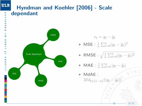
Hyndman and Koehler [2006] - Scaledependant

Scale dependant

MSE

RMSE

MAE

MdAEet = yt − yt

I MSE : 1n

∑nt=0(yt − yt)2

I RMSE :√

1n

∑nt=0(yt − yt)2

I MAE : 1n

∑nt=0 |yt − yt|

I MdAE :Mdt∈{1···n}(|yt − yt|)

29/32

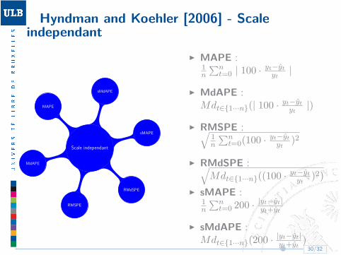
Hyndman and Koehler [2006] - Scaleindependant

Scale independant

MAPE

MdAPE

RMSPE

RMdSPE

sMAPE

sMdAPE

I MAPE :1n

∑nt=0 | 100 · yt−yt

yt|

I MdAPE :Mdt∈{1···n}(| 100 · yt−yt

yt|)

I RMSPE :√1n

∑nt=0(100 · yt−yt

yt)2

I RMdSPE :√Mdt∈{1···n}((100 · yt−yt

yt)2)

I sMAPE :1n

∑nt=0 200 · |yt−yt|

yt+yt

I sMdAPE :Mdt∈{1···n}(200 · |yt−yt|

yt+yt)30/32

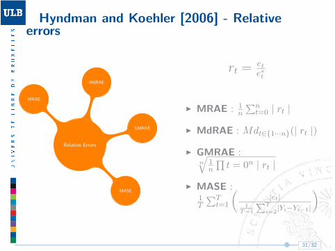
Hyndman and Koehler [2006] - Relativeerrors

Relative Errors

MRAE

MdRAE

GMRAE

MASE

rt = et

e∗t

I MRAE : 1n

∑nt=0 | rt |

I MdRAE : Mdt∈{1···n}(| rt |)

I GMRAE :n

√1n

∏t = 0n | rt |

I MASE :1T

∑Tt=1

(|et|

1T −1

∑T

i=2|Yi−Yi−1|

)

31/32

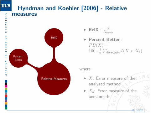
Hyndman and Koehler [2006] - Relativemeasures

Relative Measures

RelX

Percent-Better

I RelX : XXbench

I Percent Better :PB(X) =100 · 1

n

∑forecasts I(X < Xb)

where

I X: Error measure of theanalyzed method

I Xb: Error measure of thebenchmark

32/32