machine learning and multi-criteria decision analysis in...
TRANSCRIPT

Självständigt arbete på avancerad nivå Independent degree project - second cycle Civilingenjör, Industriell ekonomi Master of Science in Industrial Engineering and Management Machine learning and Multi-criteria decision analysis in healthcare A comparison of machine learning algorithms for medical diagnosis Victoria Hjalmarsson

Machine learning and Multi-criteria decision analysis in healthcare
Victoria Hjalmarsson 2018-06-11
ii
MITTUNIVERSITETET Avdelning för informations- och kommunikationssystem Examinator: Katarina Lindblad-Gidlund, [email protected] Handledare: Leif Olsson, [email protected] Författare: Victoria Hjalmarsson, [email protected] Utbildningsprogram: Civilingenjör Industriell ekonomi, 300 hp Huvudområde: Examensarbete inom industriell ekonomi, 30 hp Termin, år: 10, 2018
Machine learning and Multi-criteria decision analysis Abstract in healthcare
Victoria Hjalmarsson 2018-06-11
iii
Abstract Medical records consist of a lot of data. Nevertheless, in today’s digitized society it is difficult for humans to convert data into information and recognize hidden patterns. Effective decision support tools can assist medical staff to reveal important information hidden in the vast amount of data and support their medical decisions. The objective of this thesis is to compare five machine learning algorithms for clinical diagnosis. The selected machine learning algorithms are C4.5, Random Forest, Support Vector Machine (SVM), k-Nearest Neighbor (kNN) and Naïve Bayes classifier. First, the machine learning algorithms are applied on three publicly available datasets. Next, the Analytic hierarchy process (AHP) is applied to evaluate which algorithms are more suitable than others for medical diagnosis. Evaluation criteria are chosen with respect to typical clinical criteria and were narrowed down to five; sensitivity, specificity, positive predicted value, negative predicted value and interpretability. Given the results, Naïve Bayes and SVM are given the highest AHP-scores indicating they are more suitable than the other tested algorithm as clinical decision support. In most cases kNN performed the worst and also received the lowest AHP-score which makes it the least suitable algorithm as support for medical diagnosis.
Keywords: Analytical Hierarchy Process, Data mining, Healthcare management, MCDA

Machine learning and Multi-criteria decision analysis Table of Contents in healthcare
Victoria Hjalmarsson 2018-06-11
iv
Table of Content
Abstract ................................................................................................ iii 1 Introduction .................................................................................... 1
1.1 Overall objective.......................................................................... 2 1.2 Detailed problem statement ........................................................ 3 1.3 Scope .......................................................................................... 3
2 Theory ............................................................................................. 4 2.1 Machine learning ......................................................................... 4
2.1.1 Supervised and unsupervised machine learning................... 5 2.1.2 Machine learning algorithms ................................................. 6 2.1.3 Evaluation metrics ............................................................... 12 2.1.4 Weka ................................................................................... 16
2.2 Multi-criteria decision analysis................................................... 17 2.2.1 Weighted sum model .......................................................... 18 2.2.2 Analytic hierarchy process .................................................. 18 2.2.3 Application-Oriented Validation and Evaluation & Accurate multi-criteria decision making ........................................................ 24
2.3 Statistical metrics for medical evaluation .................................. 27 2.3.1 Sensitivity and Specificity .................................................... 27 2.3.2 Positive and negative predictive value ................................ 29 2.3.3 Reliability evaluation ........................................................... 29
2.4 Previous research ..................................................................... 30 3 Method .......................................................................................... 33
3.1 Method overview ....................................................................... 33 3.2 Data and information collection ................................................. 34 3.3 Machine learning modeling ....................................................... 35
3.3.1 Choice of software .............................................................. 35 3.3.2 Choice of machine learning algorithms ............................... 35 3.3.3 Evaluation metrics ............................................................... 35 3.3.4 Choice of datasets .............................................................. 37
3.4 Analytic hierarchy process ........................................................ 40

Machine learning and Multi-criteria decision analysis Table of Contents in healthcare
Victoria Hjalmarsson 2018-06-11
v
3.4.1 Sensitivity analysis .............................................................. 41 3.5 Method discussion .................................................................... 43
4 Results .......................................................................................... 45 4.1 Machine learning modeling ....................................................... 45 4.2 Analytic Hierarchy Process ....................................................... 47
5 Analysis ........................................................................................ 52 5.1 Ethical and social aspects ......................................................... 54
6 Conclusion ................................................................................... 56 Reference ............................................................................................ 58 Appendix A – AHP .............................................................................. 65

Machine learning and Multi-criteria decision analysis Introduction in healthcare
Victoria Hjalmarsson 2018-06-11
1
1 Introduction The traditional approach to turn data into useful information implies manual analysis and interpretation by one or more analysts. As data volumes grow intensely, the traditional approach becomes expensive, slow and less accurate. Considering a growing digitized society and the rapid technical advancement, companies focus on introducing digital solutions and benefit from innovation and automation. Knowledge discovery in data such as data mining and machine learning are essential contributors towards this digital transformation. Machine learning has become a common practice in a broad range of business problems; for instance, banks use it for fraud detection, supermarkets for customer targeting and product recommendation and in healthcare it is used for several reasons of one is as diagnosis support (Brink, Richards & Fetherolf, 2017).
The task of medical diagnosis is to define the medical situation given some clinical input such as symptoms or test results (Marsh et al. 2017). The healthcare industry has successively integrated computer technologies more and more, which has led to an increased interest of conducting research on machine learning in healthcare and made it an important component to healthcare. This, because classification models developed from machine learning algorithms can assist physicians in diagnosing diseases and provide empirical support to strengthen decisions (Zhao & Wang, 2010; Triantaphyllou, 2000). Several case studies have proposed various solutions on how to integrate machine learning as an expert system to support the task of medical diagnosis. A variety of problem-solving models have been proposed; especially in combination with cancer, diabetes, heart and skin diseases (Hussain et al. 2018; Xu et al. 2017; Alzahini et al. 2014; Chang & Chen, 2009). Based on different evaluation measures, where accuracy measures are the most common ones, the best model is recommended. The major drawback from these comparison approaches are that they often are quite one-sided. Besides accuracy, factors like usability, interpretability of results, efficiency and effectiveness (e.g. ease of updating the system with new or upgraded information) may be of importance. Therefore, it is required to analyze trade-offs between multiple criteria when choosing a suitable machine learning models (Lavesson et al. 2014).
One way that is frequently used to make decisions in many areas of science and education is multi-criteria decision analysis (MCDA) which

Machine learning and Multi-criteria decision analysis Introduction in healthcare
Victoria Hjalmarsson 2018-06-11
2
includes many different techniques. The universal concept of MCDA is to rank given alternatives by weighing criteria linked to the alternatives (Triantaphyllou, 2000). In this thesis, a MCDA approach is introduced to analyze a set of machine learning algorithms applied on medical datasets to predict if an individual is sick or healthy. The objective is to evaluate the algorithm’s predictive abilities and discuss how appropriate the machine learning algorithms under evaluation are as medical support systems for physicians.
This kind of study is significant for several reasons. First, to combine the area of computer science and management, and stress the importance of collaboration between departments and the presence of diversity in goal perspectives. This means it is important to understand both the business criteria and the machine learning criteria in order to create the best model, because often the same machine learning model needs to fulfil multiple goals arising from different departments (Witten, Frank & Hall, 2011). Second, today’s digital opportunities have the potential to support clinical decision making, leading to a better healthcare including a higher quality and efficiency in the process of diagnosis. However, Information technology (IT) is currently foremost used as administration tools and not as clinical support assisting physicians. But, Sweden has a tradition of openness and also a high availability of data, which is a good starting point for encouraging for and developing clinical support tools for diagnosis (McKinsey 2016). Technologies including machine learning cannot replace a physician’s expertise, but it can support them taking care of straightforward and time consuming diagnostic tasks and also assist in more demanding procedures like medical image recognition. Thus, potential benefits are increased diagnostics quality, where process time is expected to shorten, and diagnosis’ precision is expected to increase leading to expanded patient’s safety, reduced time to treatment along with shorter treatment time. Additionally, this will lead to a more cost-effective healthcare since staff and resources can be optimized and quality increased (Jian, 2015).
1.1 Overall objective The overall aim of this thesis is to emphasize the need for a thorough multi-criteria decision analysis in relation to machine learning evaluation. The purpose is to compare machine learning concepts stated as suitable for classification problems and for medical prediction. Then,

Machine learning and Multi-criteria decision analysis Introduction in healthcare
Victoria Hjalmarsson 2018-06-11
3
discuss why certain algorithms are more appropriate to support the task of medical diagnosis and what factors may influence the ranking.
1.2 Detailed problem statement The goal is to estimate the value of different machine learning algorithms and determine which ones are suitable as medical decision support to physicians. The approach is to apply machine learning algorithms on medical datasets and analyze the algorithms and their predictive results. Next, apply MCDA modified to suit decision making for healthcare, and create a concept on how to choose the right machine learning model to support medical diagnosis. The following questions shall be answered:
I. What machine learning algorithms are suitable to support medical diagnosis?
II. How do different evaluation criteria affect the recommendation of appropriate algorithms?
1.3 Scope The scope of this thesis is a comparison of machine learning algorithms suitable for classification problems. Algorithms are chosen based on popularity and frequency found in relevant literature and research, for instance in “Top 10 algorithms in data mining” and “Data Mining Practical Machine Learning Tools and Techniques” (Wu et al. 2008; Witten, Frank & Hall, 2011). Therefore, C4.5 algorithm, Naïve Bayes Classifier, Random Forest, Support Vector Machine and k-Nearest Neighbor are taken into account.
Due to difficulties of getting access to Medical Health Records by reason of technical and privacy concerns this study is limited to examine publicly accessible datasets available online for machine learning research in medicine and healthcare (UCI Machine Learning Repository, 2018).

Machine learning and Multi-criteria decision analysis Theory in healthcare
Victoria Hjalmarsson 2018-06-11
4
2 Theory This chapter presents theory of machine learning, MCDA, methods for medical test evaluation and previous research related to this study.
2.1 Machine learning The main difference between humans and computers are that humans are able to learn from experience and computers follow instructions. Though, by implementing machine learning, it is possible to make computers learn from past experience as well. In the context of computers, prior experience is represented by stored data. The goal of this learning is to identify patterns in data and make predictions about future events. This involves methods of data mining, machine learning and statistics (Brink, Richards & Fetherolf, 2016).
To understand machine learning properly it is helpful to understand the meaning of statistics and machine learning as well and how these three disciplines overlap:
Statistics is about the numbers; it is a field of mathematics focusing on collecting, analyzing and presenting data in order to find relevant properties (Schervish, 1995).
Data mining is about building data models based on tools and principles of statistics. The purpose is to detect patterns and relationships in data extracted from large databases that can explain some phenomena (Fayyad, Piatetsky-Shapiro & Smyth 1996).
Machine learning is about constructing algorithms that allow machines to learn from previous data without being explicitly programmed. Something is said to learn when it changes behavior in a way that makes it perform better in the future. The purpose of machine learning is to iteratively learn from data and adapt in order to improve, describe data or predict outcomes (Bramer, 2016).
In conclusion, there is no clear dividing line between statistics, data mining and machine learning. Both statistics and data mining deal with explaining and understanding data, mostly based on mathematical models. The idea is to discover patterns aiming to turn stored data into useful information, but they use different approaches. In contrast, machine learning is more concerned with algorithms and automating the process of identifying patterns in data. But, statistics and data mining concepts are the foundation to machine learning algorithms and are widely used when testing and evaluating machine learning models.
Machine learning and Multi-criteria decision analysis Theory in healthcare
Victoria Hjalmarsson 2018-06-11
5
The power of machine learning is to extract information automatically and uncover patterns by modelling data, train data and then learn from that data in the interest of improving the ability of decision making (Bramer, 2016).
When working with machine learning the following three terms, concept, instance and attribute, should be clear:
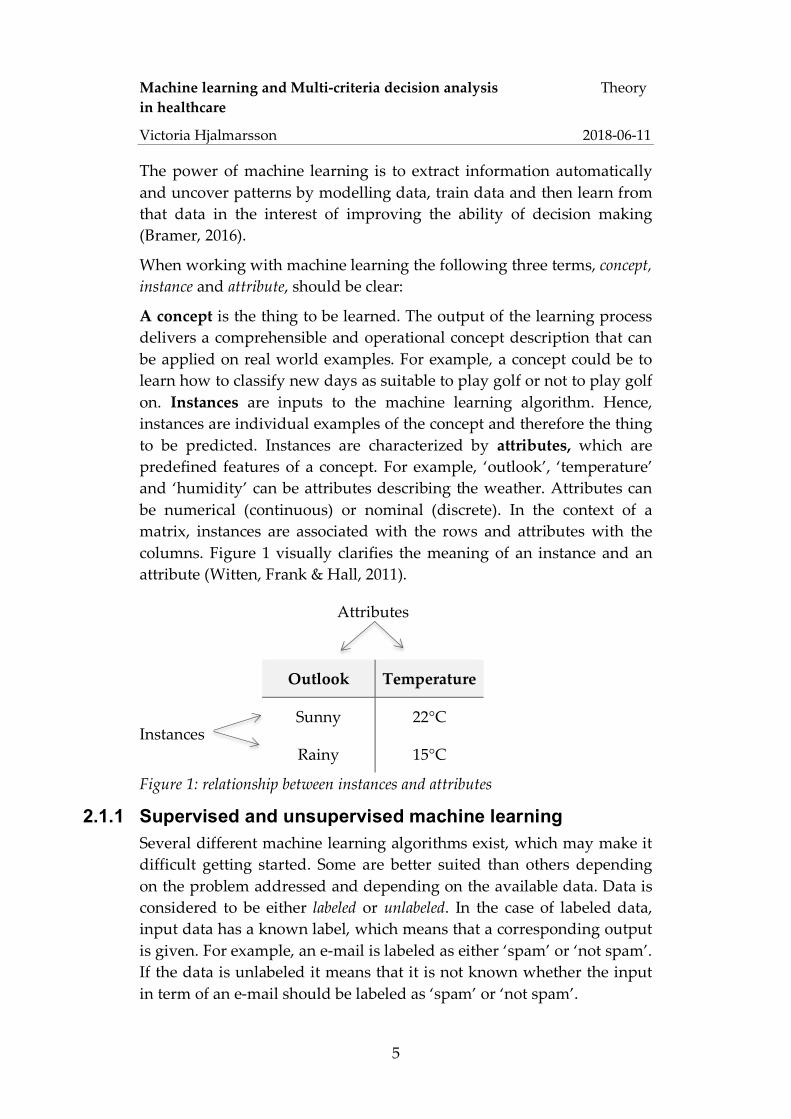
A concept is the thing to be learned. The output of the learning process delivers a comprehensible and operational concept description that can be applied on real world examples. For example, a concept could be to learn how to classify new days as suitable to play golf or not to play golf on. Instances are inputs to the machine learning algorithm. Hence, instances are individual examples of the concept and therefore the thing to be predicted. Instances are characterized by attributes, which are predefined features of a concept. For example, ‘outlook’, ‘temperature’ and ‘humidity’ can be attributes describing the weather. Attributes can be numerical (continuous) or nominal (discrete). In the context of a matrix, instances are associated with the rows and attributes with the columns. Figure 1 visually clarifies the meaning of an instance and an attribute (Witten, Frank & Hall, 2011).
Attributes
Outlook Temperature
Instances Sunny 22°C
Rainy 15°C
Figure 1: relationship between instances and attributes
2.1.1 Supervised and unsupervised machine learning Several different machine learning algorithms exist, which may make it difficult getting started. Some are better suited than others depending on the problem addressed and depending on the available data. Data is considered to be either labeled or unlabeled. In the case of labeled data, input data has a known label, which means that a corresponding output is given. For example, an e-mail is labeled as either ‘spam’ or ‘not spam’. If the data is unlabeled it means that it is not known whether the input in term of an e-mail should be labeled as ‘spam’ or ‘not spam’.

Machine learning and Multi-criteria decision analysis Theory in healthcare
Victoria Hjalmarsson 2018-06-11
6
A machine’s learning process it is often said to be either supervised or unsupervised (Han, Kamber & Pei, 2012):
Supervised learning operates on labeled datasets. The labeled dataset is split into a training - and a testing dataset to classify new instances by finding patterns. The training dataset is used to train the model by learning patters. The model is said to learn under supervision because it is being served the actual outcome of the training input. The test dataset, contains instanced which the machine has not been introduced to yet. It is used to determine how well the model has learned the given patterns, hence how well it predicts the class of new instances. Supervised learning solves classification and regression problems. Common supervised machine learning algorithms are linear regression, decision trees, support vector machines (SVM) and neural networks (Segaran, 2007).
Unsupervised learning operates on unlabeled data. There is no training dataset and no testing dataset, just a dataset. Hence, the machine learning algorithms is not trained with instances including the correct answer. Unsupervised learning is common when you are unsure what to look for. It is often used in clustering and association problems; common unsupervised machine learning algorithms are k-means and the Apriori algorithm. Assume the task is to group different fruit types, but at first, no additional information about the fruits is given. The first step is to select a piece of fruit and one of its characteristics, e.g. color. The fruits are separated based on color, resulting in for example a “red group” including apples and cherries; a “yellow group” including lemons and bananas. Next, another characteristic is chosen, e.g. size, and the fruits are rearranged. The outcome will be more specified; “red and big group” including apples; “red and small group” including cherries; “yellow and big group” including bananas and “yellow and small group” including lemons. In this manner the machine has processed the unlabeled data and has created a label for each different group. Now only one example of labeled data is needed to make the unsupervised learning algorithm effective and label unlabeled processed data (Segaran, 2007).
2.1.2 Machine learning algorithms The following section briefly presents five commonly used classification machine leaning algorithms, chosen based on popularity and how frequently they appear in context with medical diagnosis. Table 1 presents the 10 most popular algorithms obtained from a survey from

Machine learning and Multi-criteria decision analysis Theory in healthcare
Victoria Hjalmarsson 2018-06-11
7
the IEEE International Conference on Data mining (Wu et al. 2008). A more in-depth theory is presented in “Data Mining Practical Machine Learning Tools and Techniques” by Witten, Frank & Hall (2011). From previous studies it is observed that decision tree algorithms like C4.5 and Random Forest, SVM, kNN and Naïve Bayes algorithms are frequently tested classification algorithms for medical diagnosis of various diseases like cancer (Hussain et al. 2018), heart diseases (Alzahani et al. 2014; Ranganatha et al. 2013) and sepsis (Horng et al. 2017). Due to both popularity and frequent appearance in diverse medical areas, they are relevant for this study and therefore further explained below.
Table 1: Top 10 algorithms in data mining Algorithm Type
1. C4.5 algorithm Classification 2. k-Means Clustering 3. SVM Classification & Regression 4. Apriori algorithm Association rules 5. EM algorithm Statistical modeling 6. PageRank Link mining 7. AdaBoost Ensemble learning 8. k-Nearest Neighbor Classification 9. Naïve Bayes Classification 10. CART Classification
2.1.2.1 C4.5 algorithm C4.5 algorithm is a popular decision tree algorithm, which is a supervised machine learning method commonly used for classification. Decision tree algorithms follow the concept of divide and conquer. They work by recursively breaking down the problem into several sub-problems, identifying factors influencing the decision until they are simple enough to be solved directly. At last, the results of the sub-problems are merged and present a solution to the original problem. The sub-problems are arranged into a hierarchical tree structure summarized as a series of if-then statements in order to understand why a certain decision is made. To understand decision trees clearly, it is important to understand the following terminologies, which are also illustrated in figure 2 (Witten, Frank & Hall, 2011):
• Root node: Represent entire dataset and is divided into subsets; corresponds to an input attribute.

Machine learning and Multi-criteria decision analysis Theory in healthcare
Victoria Hjalmarsson 2018-06-11
8
• Splitting: Process of dividing a node into two or mode sub-nodes; each arc corresponds to a possible attribute value.
• Decision node: a node that can be split into further sub-nodes. It represents a test on an attribute, normally in terms of a true – false question and testing attributes to a constant.
• Leaf / Terminal Node: nodes that do not split; corresponds to the final predicted outcome (class / label)
• Branch / sub-tree: sub-section of the entire tree. Each branch represents a possible outcome to the test at the decision node.
• Pruning: process of reducing the size of the decision tree by removing sub-nodes from decision node. In other words, the opposite of splitting.
Figure 2: Components of a Decision Tree
Decision tree algorithms provide serval advantages; C4.5 is a simple algorithm providing quick results that users easily can understand and interpret. Next, decision trees can consider numerous possible outcomes of a decision and provide a framework to study the probability and payoffs of different decisions. Further, it can manage both nominal and numerical values and is capable of handling missing attribute values and filling them in with the most probable ones. On the other hand, results are quite imprecise compared to other machine learning techniques. Decision trees may sometimes also be unstable in the
Machine learning and Multi-criteria decision analysis Theory in healthcare
Victoria Hjalmarsson 2018-06-11
9
manner of the hierarchical structure; minor changes at the top may lead to drastic changes further down (Han, Kamber & Pei, 2012).
2.1.2.2 Random Forest Ensemble methods combine different individual classifiers and are used to increase the overall accuracy. Random forest is an ensemble method that combines several decision trees and from that forms a forest so to speak. Each decision tree is developed by attributes randomly selected at each node to determine the split. Similar to the nearest neighbor prediction approach, classification is based on majority voting where each decision tree has one vote. Compared to a single decision tree, the Random Forest algorithm reduces the problem of overfitting since results from several decision trees are combined. Further, Random Forest is flexible and does not need the input to be normalized. However, the algorithm is time-consuming and complex to construct and less intuitive compared to other algorithms (Han, Kamber & Pei, 2012).
2.1.2.3 Naïve Bayes classifier Naïve Bayes is a probabilistic classifier that uses Bayes' theorem to predict a class based on a set of attributes and probabilities of class membership. It calculates the posterior probability that a given instance belongs to a particular class. Let D be a training dataset of instances and associated class labels. Each instance is represented by an n-dimensional attribute vector, X = (x1, x2, ..., xn), describing n measurements on the instance from n attributes, A1, A2, ..., An. Next, assume there are m classes, denoted C1, C2, ..., Cm. The classifier predicts that a given instance, X, belongs to the class having the highest posterior probability, conditioned on X. That is, the Naïve Bayesian classifier predicts that instance X only belongs to class Ci if
𝑃(𝐶$|𝑋) > 𝑃)𝐶*+𝑋,𝑓𝑜𝑟1 ≤ 𝑗 ≤ 𝑚, 𝑗 ≠ 𝑖 (1)
P(Ci|X) is maximized and by Bayes’ Theorem defined as in equation 2.

Machine learning and Multi-criteria decision analysis Theory in healthcare
Victoria Hjalmarsson 2018-06-11
10
𝐵𝑎𝑦𝑒𝑠𝑡ℎ𝑒𝑜𝑟𝑒𝑚:𝑃(𝐶$|𝑋) =𝑃(𝑋|𝐶$) ∙ 𝑃(𝐶$)
𝑃(𝑋) (2)
where: C = class and X = instance,
P(X) = prior probability of instance,
P(C) = prior probability of class,
P(X|C) = Likelihood (probability of an instance given a class value)
P(C|X) = posterior probability (the probability of a class given an attribute vector)
The classifier is described as naïve since it assumes strong independence between attributes which usually is not the case on real life, and therefore seen as a drawback of the classifier. Another limitation of Naïve Bayes classifier is the so called Zero Frequency. This appears if an instance of the test dataset belongs to a class or includes an attribute value, which was not observed (has zero frequency) in the training dataset. As a consequence, the model assigns a zero probability which means the algorithms is unable to make a prediction. A common technique to overcome this issue is to use a smoothing technique; a simple and commonly used smoothing technique is called Laplace estimation. Benefits of the Naïve Bayes algorithm are that it is a simple algorithm, fast to implement and quickly predicts classes of instances of a test dataset. In cases when the assumption of independence is valid, the Naïve Bayes classifier often performs better compared to other models. It can handle both nominal and numerical values and is not sensitive to noisy data (Bramer, 2016; Ranganatha et al. 2013).
2.1.2.4 Support vector machine Support vector machine (SVM) was introduced by the work of Cortes and Vapnik (1995) on structural risk minimization and is related to the statistical learning theory (Vapnik, 1998). SVM is a classification algorithm that has gained on popularity in the past years. The goal is to find one or more optimal separating hyperplanes of the training set and maximize its margin to the support vectors. A support vector is the closest vector to the hyperplane. The margin is the distance between the two support vectors on either side of the hyperplane. To maximize the margin SVM searched for the hyperplane which is the furthest away from all data points from each class as shown in figure 3. SVM is commonly used for text classification such as spam detection and is suitable for smaller datasets containing little noise (Segaran Toby, 2007).

Machine learning and Multi-criteria decision analysis Theory in healthcare
Victoria Hjalmarsson 2018-06-11
11
Figure 3: Hyperplane with maximum margin between its support vectors,
(Han, Kamber & Pei, 2012)
The advantage of SVM is its precise results and parameters can be assigned weights, in that way more important parameters have a bigger impact than less important parameters when decisions are made. But, users have difficulties interpreting the model since the model’s way of reasoning can be challenging to understand. It is less successful on noisy datasets (Segaran, 2007).
2.1.2.5 Nearest neighbor k-Nearest-Neighbor (kNN) is a popular and simple instance-based learning algorithm. It follows the supervised learning principle and therefore uses training - and test datasets to classify instances based on similarities. The general idea is to compare new instances to existing training data and categorize them based on similarities. Usually, a distance function, normally the Euclidean function, is applied to determine which training instance is closest to the new instances and consequently assign the new instance to the same class, hence its nearest neighbor. The letter k referrers to the k nearest neighbors on which the classifier will base its predictions on. For instance, if k equals five, then the kNN-algorithm will look at the five closest training instances to the new instance. The algorithm then decides, by a majority vote, to which class the new instance belongs. Since kNN uses majority voting, it is favorable to choose k to be an odd number. This method is sometimes

Machine learning and Multi-criteria decision analysis Theory in healthcare
Victoria Hjalmarsson 2018-06-11
12
referred to as ‘lazy learning’ because the training phase is skipped, and instead new instances are directly compared to known instances. Instance based learning is effective for pattern recognition and is often used in chemical and biological structure analysis because of its adaptivity. However, a drawback is its highly sensitivity towards random variation, noisy and missing data, which reduces its predictive abilities (Han, Kamber & Pei, 2012; Bramer, 2016).
2.1.3 Evaluation metrics The main goal is to produce a generalized predictive model that is not exposed to overfitting. Machine learning models are evaluated using different statistical measures and with respect to the business problem. The most common metric is accuracy and error rate, but there are many more to choose from. Before explaining different metrics, the following terms need to be clear (Japkowicz & Shah, 2011):
I. Positive instances (P) or just Positives are instances belonging to the main class. For instance, a dataset containing class 1, ‘true’, and class 0, ‘false’, the main class corresponds to instances classified as class 1.
II. Negative instances (N) or just Negatives are instances belonging to the other classes.
III. True Positives (TP) are actual positive instances that are correctly predicted by the classification model.
IV. True Negatives (TN) are actual negative instances correctly predicted as negatives by the classifier.
V. False Positives (FP) are negative instances which have incorrectly been predicted as positives by the classifier.
VI. False Negatives (FN) are positive instances which have incorrectly been predicted as negatives by the classifier.
VII. Confusion matrix is a tool for analyzing how well a classifier can identify instances of different classes. It summarizes the above terminologies visually into a matrix shown in table 2. The number of TP and TN reflects how often the classifiers labels something correctly and FP and FN how often it labels something wrong. For a classifier to present good accuracy, ideally most of the instances would be denoted along the diagonal of the confusion matrix and remaining entries being close to zero. That is, FP and FN are zero. The grey entries of the confusion matrix in

Machine learning and Multi-criteria decision analysis Theory in healthcare
Victoria Hjalmarsson 2018-06-11
13
table 2 present additional rows or columns which do not necessarily need to be included; P′ is the number of instances that were labeled as positives (TP+FP) by the machine learning model and N′ is the number of instances that were predicted as negative (TN + FN). The total number of instances is TP + TN + FP + TN, or P+N, or P′ +N′.
Table 2: A general confusion matrix
Predicted class
Actual class
yes no Total
yes TP FN P
no FP TN N
Total P’ N’ P+N
Common evaluation metrics are (Japkowicz & Shah, 2011):
Accuracy, also called recognition rate, refers to the percentage of correctly classified instances. It is calculated as shown in equation 3.
𝐴𝑐𝑐𝑢𝑟𝑎𝑐𝑦 = 𝑇𝑃 + 𝑇𝑁𝑇𝑜𝑡𝑎𝑙 (3)
where Total = total number of instances in dataset
Error rate implies the rate of misclassifications, thus the percentage of instances that have been incorrectly classified by the classifier. Equation 4 presents a way to calculate the error rate.
𝐸𝑟𝑟𝑜𝑟𝑟𝑎𝑡𝑒 = 𝐹𝑃 + 𝐹𝑁𝑇𝑜𝑡𝑎𝑙 (4)
Sensitivity, also called recall, calculates the true positive rate according to equation 5. That is, the proportion of positive instances in the test dataset that are correctly predicted as positives.
𝑆𝑒𝑛𝑠𝑖𝑡𝑖𝑣𝑖𝑡𝑦 = 𝑇𝑃
𝑇𝑃 + 𝐹𝑁 =𝑇𝑃𝑃 (5)
Specificity is a measure of the true negative rate. Hence, an estimation of the probability of negative labels being correctly identified as negative instances. It is computed according to equation 6.

Machine learning and Multi-criteria decision analysis Theory in healthcare
Victoria Hjalmarsson 2018-06-11
14
𝑆𝑝𝑒𝑐𝑖𝑓𝑖𝑐𝑖𝑡𝑦 = 𝑇𝑁𝑁 (6)
False positive rate (FPR) represents the probability that the classifiers predict a false positive and is calculated as shown in equation 7.
𝐹𝑃𝑅 = 1 − 𝑆𝑝𝑒𝑐𝑖𝑓𝑖𝑐𝑖𝑡𝑦𝑜𝑟𝐹𝑃
𝐹𝑃 + 𝑇𝑁 (7)
Precision, also called positive predicted value, is an evaluation of exactness. In other words, precision specifies the proportion of instances labeled as positives in the test dataset that are actually positives.
𝑃𝑟𝑒𝑐𝑖𝑠𝑖𝑜𝑛 = 𝑇𝑃
𝑇𝑃 + 𝐹𝑃 =𝑇𝑃𝑃′
(8)
Kappa value is a statistical measure for reliability that compares the observed accuracy defined in equation 3 with random chance, (also called expected accuracy). The value lies in the range [0,1]. If the value is equal to one, it means perfect agreement between the machine learning model and the actual outcome of the test dataset. More detailed description of different kappa values are presented in table 3. The equation is most easily explained through the confusion matrix in table 2.
𝐾𝑎𝑝𝑝𝑎 = 𝑎𝑐𝑐𝑢𝑟𝑎𝑐𝑦 − 𝑒𝑥𝑝𝑒𝑐𝑡𝑒𝑑𝑎𝑐𝑐𝑢𝑟𝑎𝑐𝑦
1 − 𝑒𝑥𝑝𝑒𝑐𝑡𝑒𝑑𝑎𝑐𝑐𝑢𝑟𝑎𝑐𝑦 (9)
𝐸𝑥𝑝𝑒𝑐𝑡𝑒𝑑𝑎𝑐𝑐𝑢𝑟𝑎𝑐𝑦 = 𝑃U ∗ 𝑃 + 𝑁U ∗ 𝑁 (10)
Table 3: Meaning of different Kappa values Kappa value Degree of agreement
0.00 – 0.20 bad 0.21 – 0.40 weak 0.41 – 0.60 moderate 0.61 – 0.80 good 0.81 – 1.00 very good
Tenfold cross-validation is a common validation method to prevent a prediction model from overfitting. K-fold cross-validation splits the dataset into k parts. Thus, tenfold cross- validation splits the dataset into 10 parts. Each part is in turns used for testing and the rest for training

Machine learning and Multi-criteria decision analysis Theory in healthcare
Victoria Hjalmarsson 2018-06-11
15
hence the process is repeated k times until each set has been used as a test dataset. The process is summarized in four steps:
a. Decide a number of folds; k = 10 à tenfold cross-validation
b. Split the dataset intro k approximately equal parts: each set is used in turns for testing and remainder for training
c. Repeat the procedure k times
d. Error rate is the average of the 10 errors from each iteration
𝐸𝑟𝑟𝑜𝑟𝑟𝑎𝑡𝑒 =1𝑘X𝑒$
Y
$Z[
→110X𝑒$
[^
$Z[
(11)
Receiver Operation Characteristic curve and Area under Curve
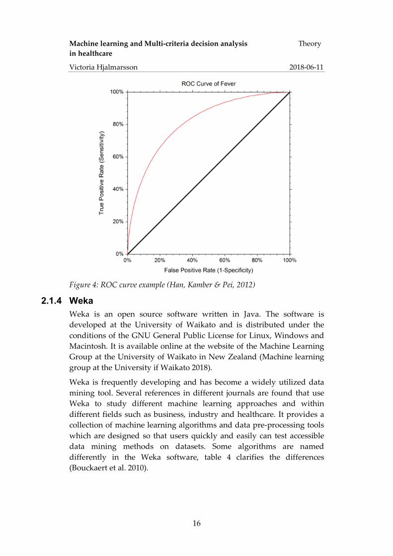
A Receiver Operating Characteristic (ROC) curve is a tool to graphically illustrate performance of a binary classifier. It illustrates the trade-off between the true positive rate (sensitivity) and the false positive rate (1-specificity) at different thresholds. That is, the balance between the rate at which the classifier is able to accurately predict positive instances versus the rate at which it mistakenly labels negative instances as positives at different sample sizes of the dataset. The accuracy of the classifier is calculated by the area under the curve (AUC). Thus, the greater the area under the ROC curve, the more accurate the classification model; a model with perfect accuracy will have an AUC equal to 1.0 (Han et al. 2012). Figure 6 present an example of a ROC curve, which is illustrate by the red line. The black line represents a random guess, where the chance is equality likely to predict a true positive as it is to predict a. false positive. The AUC of the random guess (black diagonal line) is equal to 0.5. From this it becomes clear that the closer the AUC value is to 0.5 the less accurate the model (Fawcett, 2006).
Machine learning and Multi-criteria decision analysis Theory in healthcare
Victoria Hjalmarsson 2018-06-11
16
Figure 4: ROC curve example (Han, Kamber & Pei, 2012)
2.1.4 Weka Weka is an open source software written in Java. The software is developed at the University of Waikato and is distributed under the conditions of the GNU General Public License for Linux, Windows and Macintosh. It is available online at the website of the Machine Learning Group at the University of Waikato in New Zealand (Machine learning group at the University if Waikato 2018).
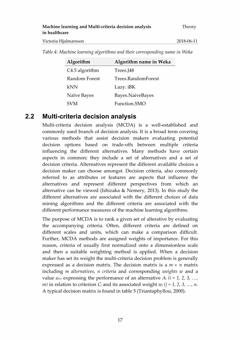
Weka is frequently developing and has become a widely utilized data mining tool. Several references in different journals are found that use Weka to study different machine learning approaches and within different fields such as business, industry and healthcare. It provides a collection of machine learning algorithms and data pre-processing tools which are designed so that users quickly and easily can test accessible data mining methods on datasets. Some algorithms are named differently in the Weka software, table 4 clarifies the differences (Bouckaert et al. 2010).
Machine learning and Multi-criteria decision analysis Theory in healthcare
Victoria Hjalmarsson 2018-06-11
17
Table 4: Machine learning algorithms and their corresponding name in Weka
Algorithm Algorithm name in Weka
C4.5 algorithm Trees.J48
Random Forest Trees.RandomForest
kNN Lazy. iBK
Naïve Bayes Bayes.NaiveBayes
SVM Function.SMO
2.2 Multi-criteria decision analysis Multi-criteria decision analysis (MCDA) is a well-established and commonly used branch of decision analysis. It is a broad term covering various methods that assist decision makers evaluating potential decision options based on trade-offs between multiple criteria influencing the different alternatives. Many methods have certain aspects in common; they include a set of alternatives and a set of decision criteria. Alternatives represent the different available choices a decision maker can choose amongst. Decision criteria, also commonly referred to as attributes or features are aspects that influence the alternatives and represent different perspectives from which an alternative can be viewed (Ishizaka & Nemery, 2013). In this study the different alternatives are associated with the different choices of data mining algorithms and the different criteria are associated with the different performance measures of the machine learning algorithms.
The purpose of MCDA is to rank a given set of alterative by evaluating the accompanying criteria. Often, different criteria are defined on different scales and units, which can make a comparison difficult. Further, MCDA methods are assigned weights of importance. For this reason, criteria of usually first normalized onto a dimensionless scale and then a suitable weighting method is applied. When a decision maker has set its weight the multi-criteria decision problem is generally expressed as a decision matrix. The decision matrix is a m ´ n matrix including m alternatives, n criteria and corresponding weights w and a value amn expressing the performance of an alternative Ai (i = 1, 2, 3, …, m) in relation to criterion Cj and its associated weight wj (j = 1, 2, 3, …, n. A typical decision matrix is found in table 5 (Triantaphyllou, 2000).

Machine learning and Multi-criteria decision analysis Theory in healthcare
Victoria Hjalmarsson 2018-06-11
18
Table 5: A general decision matrix
Criteria Alternatives C1
(w1 C2 w2
C3 w3
… …
Cn wn)
A1 a11 a12 a13 … a1n A2 a21 a22 a23 … a2n . . .
.
.
.
.
.
.
.
.
.
.
.
.
.
.
. Am am1 am2 am3 … amn
There are many ways to classify and choose appropriate MCDA models (Triantaphyllou, 2000). For this study a closer look is taken at methods that are stated to suit decision making in healthcare and found in previous research on how to integrate MCDA with the area of machine learning.
2.2.1 Weighted sum model Weighted sum model (WSM) is the earliest and one of the most frequently used MCDA methods. The model is based on the assumption of additive utility, which assumes that the total value of each alternative is equal to the sum of the product presented in equation 12. The best alternative is the one with the maximum value. The notation follows the decision matrix structure explained in table 5 (Fishburn, 1967).
𝐴$,_`abcdef =X𝑎$*𝑤*
h
*Z[
, 𝑓𝑜𝑟𝑖 = 1,2,3,… ,𝑚 (12)
2.2.2 Analytic hierarchy process The Analytic Hierarchy Process (AHP), introduced by Thomas Saaty (1977) in the 1970s, is a MCDA method which has been extensively studied and gained on popularity in different fields such as government, industry, healthcare, and education (Li, Zhang & Chu, 2012; Marsh et al. 2017). Countless references in several journals are found that use AHP in different fields like Socio-Economic Planning Science, European Journal of Operational research and Mathematical and Computer Modelling (Brunnelli, 2015; Vaidya & Kumar, 2004; Zeshui & Cuiping, 1999). AHP has also become a popular method to combine with other MCDA methods and to apply when deciding what machine

Machine learning and Multi-criteria decision analysis Theory in healthcare
Victoria Hjalmarsson 2018-06-11
19
learning algorithms to choose (Khanmohammadi & Rezaeiahari, 2014; Lavesson & Davidsson, 2008; Ali, Lee & Chung; 2017).
AHP assists decision makers to prioritize and proposing the best decision by helping them to capture subjective as well as objective aspects of a decision problem and adjust the decision accordingly. This, by reducing the complexity of decision problem into a sequence of pairwise comparisons, and then merging the results. The process is summarized into six sequential steps (Mu & Pereyra-Rojas, 2017):
Step 1 - Create a hierarchy
Structure the decision problem as a hierarchy of goal, criteria and alternatives, as shown in figure 5. Suppose the goal is ‘to buy a car’, related criteria are for example ‘cost’, ‘comfort’ and ‘safety’ and alternatives reflect the different car options, for example Mercedes, Toyota and BMW. The hierarchy structure provides a comprehensive overview of the decision problem, how to represent and quantify its elements, how these elements are related to the overall goals, and how alternatives can be evaluated. Another advantage is that elements of the hierarchy can relate to any aspect of the decision problem, that is both tangible or intangible aspects may be included.
Figure 5: Simple AHP hierarchy structure

Machine learning and Multi-criteria decision analysis Theory in healthcare
Victoria Hjalmarsson 2018-06-11
20
Step 2 – Employ a pairwise comparison
Each criterion is assigned a relative weight which reflects the priority in terms of importance amongst all criteria. Weights are derived by pairwise comparing the relative priority of two criteria at a time. The numerical scale developed by Saaty (2012) for comparison as shown in table 6 is applied for the pairwise comparison:
a) Establish a pairwise comparison matrix as in table 7 using Saaty’s comparison scale presented in table 6. Table 7 presents the relative pairwise priority for each criterion, which shows that criterion 1 is ‘moderate more important’ than criterion 2 and ‘extremely more important’ than criterion 3. It also becomes clear from the perspective of criterion 2 that the value corresponding to criterion 1 is the inverse of importance stated from the perspective of criterion 1.
b) Estimate relative weights of each criterion which is done by normalizing the comparison matrix of table 7. First, calculate the sum of each column, which corresponds to the values of the last row in table 7. Second, divide each cell of the same column by the sum of that column; results are presented in table 8. Third, calculate the average value of each row which represents the final weight of each criterion. Hence, criterion 1 is assigned a weight of 0.67, criterion 2 a weight of 0.27 and criterion 3 a weight of 0.06.
Table 6: Saaty's scale for pairwise comparision
Intensity of Importance Definition 1 Equal importance 3 Moderate more important 5 Strongly more important 7 Very strongly more important 9 Extremely more important
Intensities of 2, 4, 6, 8 may be used to express intermediate values.
Table 7: Comparison matrix of criteria Criterion 1 Criterion 2 Criterion 3
Criterion 1 1 3 9
Criterion 2 1/3 1 5
Criterion 3 1/9 1/5 1
Sum of column 1.44 4.20 15.00

Machine learning and Multi-criteria decision analysis Theory in healthcare
Victoria Hjalmarsson 2018-06-11
21
Table 8: Normalized comparison matrix including final weights of each criterion
Criterion 1 Criterion 2 Criterion 3 Weight
Criterion 1 0.69 0.71 0.60 0.67
Criterion 2 0.23 0.24 0.33 0.27
Criterion 3 0.08 0.05 0.07 0.06
Step 3 – Check for consistency in judgement.
In decision analysis consistency is a fundamental term that needs to be considered. Suppose a decision maker prefers alternative A twice as much as B and B twice as much as C. In order to be consistent, mathematically A is preferred four times as much as C. AHP contains a technique to determine how consistent or inconsistent a decision maker’s judgement is when defining the priorities in the comparison matrix (table 7). This, because priorities are derived by subjective preferences of decision makers. The technique calculates a Consistency ratio (CR) which compares the calculated Consistency index (CI) of the comparison matrix in question with a CI of a random-like matrix denoted as RI. The random-like matrix is a comparison matrix that contains randomly assigned priorities and therefore it is expected to be highly inconsistent. The RI reflects the average CI of 500 random-like matrices. Table 9 presents estimated RI values of matrices of different sizes provided by Saaty (2012). The CI is obtained by the following calculations:
a) Compute the weighted sum of each row (see equation 1) from the comparison matrix in table 7. Result is presented in table 10.
b) Calculate l: Divide the weighted sum by the corresponding weight of each criterion. For criterion 1 that is 2.04/0.67 = 3.06 as presented in table 10.
c) Calculate the average l of all criteria as presented in table 10.
d) Calculate the consistency index CI according to equation 13.
𝐶𝐼 =
𝜆nofenpf − 𝑛𝑛 − 1
where n = number of compared criteria (13)
e) Calculate the Consistency ratio CR according to equation 14, where the value of RI is found in table 9.

Machine learning and Multi-criteria decision analysis Theory in healthcare
Victoria Hjalmarsson 2018-06-11
22
𝐶𝑅 =
𝐶𝐼𝑅𝐼
where, 𝐶𝑅 = q ≤ 0.10 → 𝑎𝑐𝑐𝑒𝑝𝑡𝑎𝑏𝑙𝑒> 0.10 → 𝑖𝑛𝑐𝑜𝑛𝑠𝑖𝑠𝑡𝑒𝑛
(14)
Table 9: Consistency indices RI for radom-like comparison matrices n (number of compared elements) 3 4 5 6 7 8
RI 0.58 0.90 1.12 1.24 1.32 1.41
Table 10: Comparison matrix including weighted sum and l
Criterion 1
w1 = 0.67
Criterion 2
w2 = 0.27
Criterion 3
w1 = 0.06
Weighted sum
l
Criterion 1 0.67 0.80 0.57 2.04 3.06
Criterion 2 0.22 0.27 0.32 0.81 3.03
Criterion 3 0.07 0.05 0.06 0.19 3.01
Average l 3.03
The CI and the CR for this example is calculated as shown in equation 15 and 16 respectively.
𝐶𝐼 =3.03 − 33 − 1 = 0.01 (15)
𝐶𝑅 =0.010.58 = 0.03 (16)
The calculated consistency ratio CR is less than 0.10 which indicates that the comparison matrix established by a decision maker is reasonably consistent according to Saaty’s definition. This means the AHP analysis may continue without having to adjust any priorities in table 7.
Step 4 – Determine local priorities among the alternatives
The relative local priorities of the alternatives need to be defined with respect to each criterion. This is called the local priorities since these are only valid regarding each particular criterion.
Similar to step 2, each alternative needs to be pairwise compared, and with respect to each criterion. A decision problem with three alternatives requires three comparisons for each criterion. Thus, comparing alternative A with B, B with C and A with C for each

Machine learning and Multi-criteria decision analysis Theory in healthcare
Victoria Hjalmarsson 2018-06-11
23
criterion. The main question to ask for each comparison matrix is: With respect to the jth criterion, which alternative is preferred?
a. Establish a pairwise comparison matrix as explained in step 2 to compare the alternatives. Table 11 presents an example based on criteria 1 and a decision problem including two alternatives. Alternative 1 is ‘very strongly more important’ than alternative 2.
b. Calculate the local weights of each alternative by normalizing the comparison matrix of table 11 as explained in step 2. First, calculate the sum of each column. Second, divide each cell by the sum of that column. Third, calculate the average value of each row, which represents the local priority of each alternative. Column 4 in table 12 present the local priority of both alternatives with respect to criterion 1. This process is repeated for each criterion.
Table 11: Comparison matrix of alternatives
Criterion 1 Alternative 1 Alternative 2
Alternative 1 1 7
Alternative 2 1/7 1
Sum of column 1.14 8.00
Table 12: Normalized comparison matrix including final weights of each alternative
Criterion 1 Alternative 1 Alternative 2 local priority
Alternative 1 0.88 0.88 0.88
Alternative 2 0.13 0.13 0.13
Step 5 – Estimate the overall preferences for each alternative
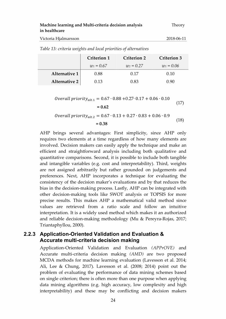
The overall priority of each alternative is determined by calculating the weighted sum including the criteria weights and the local priorities of each alternative. Consider the local priorities for alternatives and criterion weights presented in table 13. The overall preferences are calculated as the weighted sum; equations 17 and 18 presents the calculations for alternative 1 and alternative 2 respectively.
Machine learning and Multi-criteria decision analysis Theory in healthcare
Victoria Hjalmarsson 2018-06-11
24
Table 13: criteria weights and local priorities of alternatives
Criterion 1
w1 = 0.67
Criterion 2
w2 = 0.27
Criterion 3
w1 = 0.06
Alternative 1 0.88 0.17 0.10
Alternative 2 0.13 0.83 0.90
𝑂𝑣𝑒𝑟𝑎𝑙𝑙𝑝𝑟𝑖𝑜𝑟𝑖𝑡𝑦nwx.[ = 0.67 ∙ 0.88 +0.27∙ 0.17 + 0.06 ∙ 0.10
= 0.62 (17)
𝑂𝑣𝑒𝑟𝑎𝑙𝑙𝑝𝑟𝑖𝑜𝑟𝑖𝑡𝑦nwx.{ = 0.67 ∙ 0.13 + 0.27 ∙ 0.83 + 0.06 ∙ 0.9
= 0.38 (18)
AHP brings several advantages: First simplicity, since AHP only requires two elements at a time regardless of how many elements are involved. Decision makers can easily apply the technique and make an efficient and straightforward analysis including both qualitative and quantitative comparisons. Second, it is possible to include both tangible and intangible variables (e.g. cost and interpretability). Third, weights are not assigned arbitrarily but rather grounded on judgements and preferences. Next, AHP incorporates a technique for evaluating the consistency of the decision maker’s evaluations and by that reduces the bias in the decision-making process. Lastly, AHP can be integrated with other decision-making tools like SWOT analysis or TOPSIS for more precise results. This makes AHP a mathematical valid method since values are retrieved from a ratio scale and follow an intuitive interpretation. It is a widely used method which makes it an authorized and reliable decision-making methodology (Mu & Pereyra-Rojas, 2017; Triantaphyllou, 2000).
2.2.3 Application-Oriented Validation and Evaluation & Accurate multi-criteria decision making Application-Oriented Validation and Evaluation (APPrOVE) and Accurate multi-criteria decision making (AMD) are two proposed MCDA methods for machine learning evaluation (Lavesson et al. 2014; Ali, Lee & Chung, 2017). Lavesson et al. (2008; 2014) point out the problem of evaluating the performance of data mining schemes based on single criterion; there is often more than one purpose when applying data mining algorithms (e.g. high accuracy, low complexity and high interpretability) and these may be conflicting and decision makers

Machine learning and Multi-criteria decision analysis Theory in healthcare
Victoria Hjalmarsson 2018-06-11
25
might weight them differently. They suggest an application-oriented approach, named APPrOVE, inspired by several well-established MCDA methods including AHP and Large Preference Relation. The benefits from evaluating a data mining algorithm’s performance based on multi-criteria and the APPrOVE method is a customized evaluation, balancing trade-offs between multiple criteria rather than maximizing only one. This leads to more precise decisions because all goals are considered and analyzed, and criteria are weighted accordingly. APPrOVE involved four steps; 1) Identify quality attributes; 2) Prioritize attributes; 3) Metric selection; 4) Validation and evaluation (Lavesson et. al. 2014).
Ali, Lee & Chung (2017) developed the concept of APPrOVE further to what they named Accurate multi-criteria decision making (AMD) which is a methodology for recommending machine learning algorithms. Like Lavesson et al. (2008; 2014) they state the problem of current MCDA methods used in data mining lack suitable evaluation criteria; decision makers often don’t know the difference between different evaluation metrics and criteria are often equally prioritized. Further the AMD concept is quite similar to APPrOVE and is inspired by the concept of AHP, TOPSIS and inclusion of multiple quality attributes. It is broken down into four sequential phases:
I. Define the goal and objective for the data mining algorithms.
II. Select criteria and weights; first decision makers select relevant criteria in terms of ‘quality meta metrics’ (QMM) that match the goal and objectives. Next, appropriate evaluation metrics for each of the QMMs are chosen and lastly each metric is assigned a weight. This second phase matches step 1) and 2) of APPrOVE. Eight QMMs are identified, which are similar to the quality attributes options found in Lavesson et al. (2014):
a. Correctness measures the algorithm’s accuracy or error rate. Suggested evaluation metrics are amongst others accuracy, precision, or error rates like false positive rate.
b. Complexity refers to either computational complexity in terms of e.g. elapsed time or memory space complexity like tree size or number of rules.
c. Responsiveness determines computational efficiency regarding testing and execution time.

Machine learning and Multi-criteria decision analysis Theory in healthcare
Victoria Hjalmarsson 2018-06-11
26
d. Consistency denotes the level of performance on a certain dataset and is determined by the standard deviation.
e. Interpretability; compared to the other QMMS this is a more subjective estimation of interestingness and interpretability from a user’s perspective. Hence, it addresses how well the classifier’s reasoning and conclusion is understood by the user.
f. Reliability defines how trustworthy an algorithm is. Similar to correctness suitable metrics are error estimations, otherwise entropy is also a proposition.
g. Robustness considers the algorithm’s performance in relation to noisy data and missing values. For example, by examining sensitivity and AUC.
h. Separability is similar to robustness and is examined by visualizing ROC and AUC.
When relevant QMMs and corresponding evaluation metrics are selected, weights are assigned. Weighting follows the concept of AHP weighting explained in section 2.2.2.
III. Measure the algorithm’s performance; performance results of each QMM is generated for the algorithms that are being evaluated. Statistical significance and fitness tests are conducted. Results are summarized into a decision matrix including all criteria and algorithms.
IV. Rank and choose algorithms based on their performance results and criteria weights which is expressed as an aggregated score of multiple metrics. The evaluation process is inspired by TOPSIS which ranks alternatives according to their relative closeness to the ideal algorithm, a detailed description is found in (Triantaphyllou, 2000). Afterwards, the top m algorithms are presented for the user’s application.
After empirical analysis, experiments and comparisons with general accepted MCDA methods authors conclude that these proposed methods (APPrOVE and ADM) provide feasible methodologies and good results.

Machine learning and Multi-criteria decision analysis Theory in healthcare
Victoria Hjalmarsson 2018-06-11
27
2.3 Statistical metrics for medical evaluation In diagnostics it is important to have as safe tests as possible, that is results need to be certain and of high probabilities. A good test should be sensitive so that as few sick patients as passible are overlooked and simultaneously return as few false alerts as possible. Generally, test results are split into positive test (indicates some disease) and negative test (indicates health). The reliability of a test is crucial in order to draw conclusions from it. Test results are generally split into four categories (Ludvigsson & Ekbom, 2017; SBU, 2014):
a. True positives: sick patient classified as sick b. False positives: healthy patient classified as sick c. False negatives sick patient classified as healthy d. True negatives: healthy patient classified as healthy
The relationship between these four test results and a disease is illustrated in table 14, which reminds of a confusion matrix used in data mining explained in section 2.1.3 (Ludvigsson & Ekbom, 2017; SBU, 2014).
Table 14: Relationship between test results and disease
Positive test Negative test Sick a. True positive b. False negative
Not sick (healthy) c. False positive d. True negative
Based on these four categories, diagnostic tests are evaluated in several ways, however there are basically two main concepts that lie to ground for the remaining evaluation methods; these are sensitivity and specificity. Furthermore, the positive predictive value and the negative predictive values are major metrics as is often various reliability measures such as the kappa value (SBU, 2014).
2.3.1 Sensitivity and Specificity Sensitivity and specificity estimates how reliable a test is. In the content of clinical diagnostics sensitivity refers to the probability for a positive test result when a disease is present. Thus, sensitivity returns the proportion of sick people who correctly have been identified by a test. As explained in section 2.1 it states to the positive test rate and is calculated according to equation 5.
Specificity refers to the probability for a negative test results when the patient is healthy. Hence, the proportion of healthy patients who have

Machine learning and Multi-criteria decision analysis Theory in healthcare
Victoria Hjalmarsson 2018-06-11
28
been correctly diagnosed as not sick through a test and is calculated as presented in equation 6. Both sensitivity and specificity are defined on a range from 0 to 100. The closer to 100 the better or accurate the test, as explained via ROC curves in section 2.1 (SBU, 2014).
I some situations, sensitivity is more important while in other cases specificity might be of greater importance. Sensitivity is more central when a disease cannot be missed. For instance, life-threatening diseases that can be cured, like tuberculosis. However, a test that has to identify all sick patients often also brings along some healthy ones. Therefore, usually several tests are necessary in order to guarantee that a patient really is sick. Since a test with high specificity declares a patient to be healthy, specificity is more important in the case where physicians want to be completely sure that a person really is suffering from a disease. For example, before starting a life-threatening treatment. This means, that even though cancer is strongly suspected, a biopsy is usually established before starting the treatment (Ludvigsson & Ekbom, 2017). Table 15 presents a structure of factors that are significant for different clinical tests.
Table 15: Factors that are significant for clinical tests (SBU, 2014)
Prevalence of disease Occurrence of disease in the test group Damages of healthy being classified as ill à requirement for specificity
1. risks of treating healthy individuals 2. treatment costs 3. ethical consequences
Damages of sick being classified as healthy à requirement for sensitivity
1. risks of not getting treatment 2. population risks (infection spread) 3. genetic risks
When talking about sensitivity, specificity and ROC-curves, the term cut-off often occurs. Cut-off is the boundary between positive and negative and affects both sensitivity and specificity of a test. A low cut-off implies that all sick will be identified and therefore the test has a high sensitivity. But, at the same time some healthy patients will also be diagnosed as sick, since a high sensitivity means a low specificity leading to some healthy patients receiving a false positive test result. A high cut-off implies low sensitivity such that all sick patients are not identified. Nevertheless, physicians can be sure that all healthy patients are correctly diagnosed with a negative test results and actually are
Machine learning and Multi-criteria decision analysis Theory in healthcare
Victoria Hjalmarsson 2018-06-11
29
well. Thus, testes with a high cut-off denotes high specificity (Ludvigsson & Ekbom, 2017).
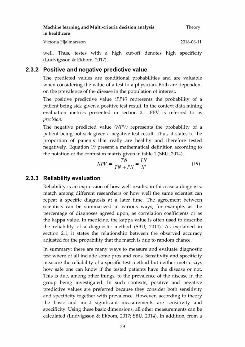
2.3.2 Positive and negative predictive value The predicted values are conditional probabilities and are valuable when considering the value of a test to a physician. Both are dependent on the prevalence of the disease in the population of interest. The positive predictive value (PPV) represents the probability of a patient being sick given a positive test result. In the context data mining evaluation metrics presented in section 2.1 PPV is referred to as precision. The negative predicted value (NPV) represents the probability of a patient being not sick given a negative test result. Thus, it states to the proportion of patients that really are healthy and therefore tested negatively. Equation 19 present a mathematical definition according to the notation of the confusion matrix given in table 1 (SBU, 2014).
𝑁𝑃𝑉 =𝑇𝑁
𝑇𝑁 + 𝐹𝑁 =𝑇𝑁𝑁′
(19)
2.3.3 Reliability evaluation Reliability is an expression of how well results, in this case a diagnosis, match among different researchers or how well the same scientist can repeat a specific diagnosis at a later time. The agreement between scientists can be summarized in various ways; for example, as the percentage of diagnoses agreed upon, as correlation coefficients or as the kappa value. In medicine, the kappa value is often used to describe the reliability of a diagnostic method (SBU, 2014). As explained in section 2.1, it states the relationship between the observed accuracy adjusted for the probability that the match is due to random chance.
In summary; there are many ways to measure and evaluate diagnostic test where of all include some pros and cons. Sensitivity and specificity measure the reliability of a specific test method but neither metric says how safe one can know if the tested patients have the disease or not. This is due, among other things, to the prevalence of the disease in the group being investigated. In such contexts, positive and negative predictive values are preferred because they consider both sensitivity and specificity together with prevalence. However, according to theory the basic and most significant measurements are sensitivity and specificity. Using these basic dimensions, all other measurements can be calculated (Ludvigsson & Ekbom, 2017; SBU, 2014). In addition, from a

Machine learning and Multi-criteria decision analysis Theory in healthcare
Victoria Hjalmarsson 2018-06-11
30
cost sensitive perspective, it is of higher cost to falsely label deadly sick patients as not sick rather than misclassify healthy patients (Han, Kamber, Pei, 2012). As a conclusion, sensitivity and specificity are considered as very important criteria, followed by first PPV and at last NPV and Kappa value.
2.4 Previous research Machine learning in health care is a topic gaining popularity amongst researchers. There are a lot of machine learning techniques and tools available. Different researchers use different approaches or compare different methods to determine which one is more suitable. This has lead in a variety of problem-solving methods. For instance, Horng et al. (2017) created a machine learning model for early sepsis detection using SVM. Their purpose was to demonstrate the benefit of including free text data, such as nurse’s triage, in addition to structured data, like vital signs and demographics. In conclusion, successively adding free text kept improving the model’s predictive ability, as well as giving a broader understanding why the patient is at the emergency department. Another research integrated machine learning algorithms like Multi-Layer perceptron and Support vector machine for breast cancer detection. They proposed a new three-class classification technique for classifying breast cancer (including classes normal, benign, malignant) which usually uses a two-class classification technique (including classes normal, abnormal). Validation results based in statistical evaluation including ROC curves and accuracy show the significance of proposed scheme as compared to existing schemes (Jadoon et al. 2017). Similarly, machine learning in terms of SVM was tested as support tool for classification of Alzheimer’s disease patients. Evaluation established ROC curve analysis present high accuracy of 0.8582. From this, authors concluded that the suggested machine learning concept is suitable as computer aided classification of Alzheimer’s disease (Jongkreangkrai et al. 2016). Another study applied machine learning algorithms like random forest and logistic regression to obtain predictive models of type 2 diabetes complications. Based on high accuracies (up to 0.838) that the different predictive models achieved and for the fact that they are easy to translate into the clinical practice these models are found to be a suitable as clinical support (Dagliati et al. 2018).
Even though it is shown that machine learning concepts present accurate predicting abilities in classifying diseases in several ways, it is not shown how accurate these abilities are relative to the abilities of

Machine learning and Multi-criteria decision analysis Theory in healthcare
Victoria Hjalmarsson 2018-06-11
31
physicians and how these proposed models affect the overall diagnosis quality. A study reviewing the effect of applying neural network methods for medical analysis addresses these thoughts. Conclusions state that machine learning schemes can support diagnosis, especially for new and rare diseases where physicians accurately diagnose 79.97 % and this level was increased to 91.1% when diagnoses were established with the support of the neural network algorithm and an expert system (Brause 2001).
Further, it is of interest to identify critical factors that are significant for medical predictions and that increase the diagnosis abilities. Above mentioned studies follow the same evaluation structure. Each study is evaluated based on accuracy in terms ROC curves analysis, success rate and averaged or balanced accuracy. A study conducted by Lavesson & Davidsson (2008) examine the problem of evaluating the performance of data mining schemes based on only one criteria such as accuracy. They propose a novel multi-criteria evaluation measure based on several well-established methods like Data Envelopment Analysis (DEA) and the Simple and Intuitive measure for MCDA (Soares, Costa & Brazdil, 2000). Results show that evaluating performance of a machine learning model based on multi-criteria provides a customized evaluation balancing the trade-off between multiple criteria rather than maximizing only one. This is significant because different business problems have different goals and therefore different criteria may be more or less important. This concept was taken further, and, in another study, they created a methodology named APPrOVE and other researchers build upon that and established an accurate multi-criterion decision-making methodology (AMD) which is presented in section 2.2. AMD empirically examines and then ranks the classification model. Ranking is established by combining a weighted average F-score, execution times of training and testing the model and consistency measures (Ali, Lee & Chung 2017; Lavesson et al. 2014).
Additionally, it is not to forget that machine learning also has its weaknesses. Where humans can rely on knowledge and experience, a machine learning model can make predictions based on existing data, hence machine learning is well suited for predictions based on already seen data. Therefore, it is quite difficult to make accurate predictions based on new data, which the computer has not seen before because it is most likely to be misinterpreted (Segaran 2007). Since the practice of medicine is continually evolving regarding new technology and social phenomena the target is not fixed. Therefore, humans’ knowledge and

Machine learning and Multi-criteria decision analysis Theory in healthcare
Victoria Hjalmarsson 2018-06-11
32
experience can be of more value for medical diagnosis than machine learning algorithms, which mainly use historical data form medical health records to find patterns. Another limit of machine learning is the risk of possible overfitting; predictions are usually based on associations without any regards to fundamental theory. If only few examples are included in the training set, outcome will possibly not reflect reality accurately (Chen & Ash, 2017). Considering these limitations, it has to be acknowledged that results from the predictive machine learning models might not always mirror reality correctly. These aspects need to be considered when evaluating whether or not a machine learning model is sufficient enough as a clinical support tool.
Previous studies state that several machine learning algorithms are suitable as clinical support tools for diagnosing different types of diseases; increased accuracy and sensitivity lead to more correct diagnoses. Yet, there is still little research conducted on how these solutions add value to healthcare and to the process of diagnosis assessment. Since previous research has resulted in a variety of possible solutions for what machine learning schemes to implement, this study is concerned with creating a concept to evaluate different models from a management point of view. The evaluation focuses on how suitable different machine learning algorithms are to support physicians to predict whether a patient is sick or healthy. This thesis evaluates and compares different machine learning algorithms using MCDA in order to reduce the bias when choosing suitable machine learning techniques for medical diagnosis. The goal is to present a method on how to choose appropriate evaluation criteria and how to include multiple criteria during evaluation of the different machine learning techniques. This research is interesting for decision makers in healthcare; on one hand as a decision support for healthcare management dealing with investment opportunities, on the other as medical classification support assisting physicians in their everyday work of diagnosing patients. The results of this study contribute with knowledge and perspectives on how machine learning algorithms can be compared and preferred, and simultaneously reducing the bias of decision makers during the decision-making process. Furthermore, it indicates what algorithms are more suitable than others for a hospital setting. Results also emphasize the need of combining the perspective of computer science with the point of view of management and decision analysis in order to achieve more accurate and efficient final decisions.

Machine learning and Multi-criteria decision analysis Method in healthcare
Victoria Hjalmarsson 2018-06-11
33
3 Method Chapters 3.1 to 3.5 describe methods used during this study. It begins with covering an overview involving the overall approach followed by methods for data and information collection. Next, it is described how machine learning algorithms and MCDA concepts are applied in this particular thesis. Finally, a detailed method discussion is presented explaining why selected methods are preferred.
3.1 Method overview This is a retrospective cohort study following a quantitative research approach including a multi-criteria decision analysis. Retrospective study means that data is collected after the incident has occurred. The researcher looks backwards, examining the situation before the outcome of interest has happened, and tries to expose potential factors which triggered the particular outcome. Retrospective investigations are typical in medical research; a cohort of individuals sharing common symptoms are compared to a different group of people who are not exposed to those symptoms, to determine a symptom’s influence on the outcome of a disease or death (Supino & Borer, 2012). Quantitative research implies quantifying data and generalizing results from a sample of the population of interest using structured techniques in order to explain or predict something using hard data and numbers. (Creswell, 2003).
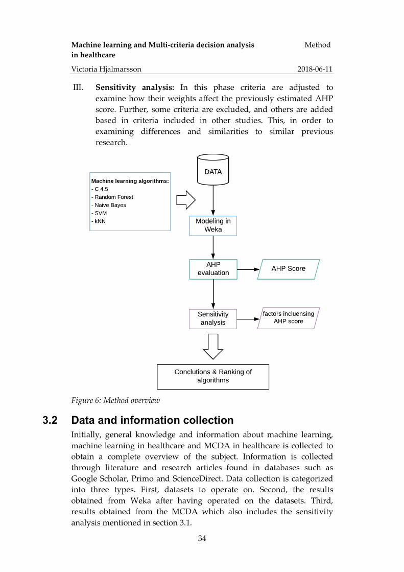
The core of this study is to run five different machine learning algorithms suited for classification and extract results from three different medical datasets. Next, use these results as input for a multi-criteria decision analysis and determine what algorithms and why are the most suitable for medical diagnostics predictions. The overall method approach is visualized in figure 6 and can be divided into three sequential phases:
I. Machine learning modeling: In this phase selected machine learning algorithms are applied on the selected datasets and run though the Weka software.
II. Multi-criteria decision analysis: In this phase the performance results and selected quality metrics are weighted, and each machine learning algorithm is assigned a score related to how suitable they are as a clinical support model.
Machine learning and Multi-criteria decision analysis Method in healthcare
Victoria Hjalmarsson 2018-06-11
34
III. Sensitivity analysis: In this phase criteria are adjusted to examine how their weights affect the previously estimated AHP score. Further, some criteria are excluded, and others are added based in criteria included in other studies. This, in order to examining differences and similarities to similar previous research.
Figure 6: Method overview
3.2 Data and information collection Initially, general knowledge and information about machine learning, machine learning in healthcare and MCDA in healthcare is collected to obtain a complete overview of the subject. Information is collected through literature and research articles found in databases such as Google Scholar, Primo and ScienceDirect. Data collection is categorized into three types. First, datasets to operate on. Second, the results obtained from Weka after having operated on the datasets. Third, results obtained from the MCDA which also includes the sensitivity analysis mentioned in section 3.1.

Machine learning and Multi-criteria decision analysis Method in healthcare
Victoria Hjalmarsson 2018-06-11
35
3.3 Machine learning modeling For each dataset the same process is repeated, and the same machine learning algorithms are applied.
3.3.1 Choice of software Weka is chosen for this thesis because it is simple tool easily understood that includes various machine learning algorithms well suited for this study. Further, Witten, Frank & Hall (2011) claims that Weka facilitates the process of applying and comparing machine learning algorithms. Thus, Weka is commonly used for comparing different algorithms (Fatima & Pasha, 2017; Othman & Yau, 2007; Soni et al. 2011; Solanki, Ashokkumar V. 2014). Algorithms are evaluated with the default setting of Weka, which is tenfold cross-validation (Machine learning group at the University if Waikato 2018).
3.3.2 Choice of machine learning algorithms Machine learning algorithms are chosen based on popularity and frequency of appearance in earlier similar studies as explained in chapter 2.1 and 2.4. Additionally, the list of appropriate machine learning algorithms are narrowed down to widely used machine learning algorithms for classification problems. The following five algorithms are selected:
a. C4.5 algorithm (Wiharto,Kusnanto&Herianto,2016) b. k-Nearest-Neighbor (Shouman,Turner&Stocker,2012) c. Naïve Bayes (Jian,Anju2015) d. Random Forest (Xuetal.2017) e. Support Vector Machine (Guyonetal.2002)
3.3.3 Evaluation metrics There is a variety of performance measures to choose from and the difficulty is to choose the appropriate ones. A common issue is that users do not comprehend the particular meaning of each performance measures and therefore struggle with choosing appropriate metrics (Ali, Lee & Chung 2017). To avoid this problem the QMMs for evaluating machine learning models presented by Ali, Lee & Chung (2017) together with the basic measures for medical evaluations presented in chapter 2.3 are considered when selecting performance metrics for this study. The selected metrics are summarized in table 16. QMMs are picked based on the given definitions in chapter 2.2.3 and how appropriate they appear to be for the machine learning task in mind. Performance metrics for
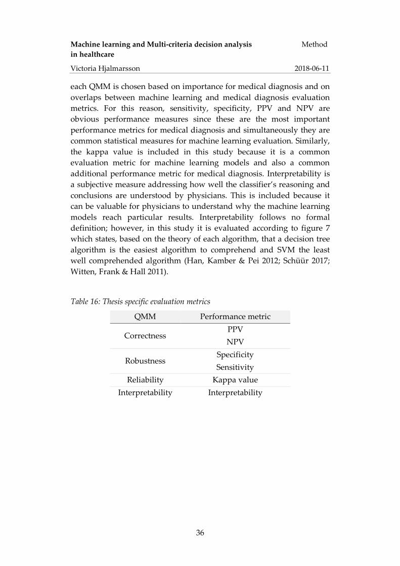
Machine learning and Multi-criteria decision analysis Method in healthcare
Victoria Hjalmarsson 2018-06-11
36
each QMM is chosen based on importance for medical diagnosis and on overlaps between machine learning and medical diagnosis evaluation metrics. For this reason, sensitivity, specificity, PPV and NPV are obvious performance measures since these are the most important performance metrics for medical diagnosis and simultaneously they are common statistical measures for machine learning evaluation. Similarly, the kappa value is included in this study because it is a common evaluation metric for machine learning models and also a common additional performance metric for medical diagnosis. Interpretability is a subjective measure addressing how well the classifier’s reasoning and conclusions are understood by physicians. This is included because it can be valuable for physicians to understand why the machine learning models reach particular results. Interpretability follows no formal definition; however, in this study it is evaluated according to figure 7 which states, based on the theory of each algorithm, that a decision tree algorithm is the easiest algorithm to comprehend and SVM the least well comprehended algorithm (Han, Kamber & Pei 2012; Schüür 2017; Witten, Frank & Hall 2011).
Table 16: Thesis specific evaluation metrics
QMM Performance metric
Correctness PPV NPV
Robustness Specificity Sensitivity
Reliability Kappa value Interpretability Interpretability

Machine learning and Multi-criteria decision analysis Method in healthcare
Victoria Hjalmarsson 2018-06-11
37
Figure 7: Comparison of interpretability and accuracy of different machine learning algorithms (Schüür, 2017)
3.3.4 Choice of datasets Since the objective of this thesis is to evaluate machine learning algorithms regarding their suitability as a support in healthcare, public available datasets for machine learning research in medicine and healthcare are examined. Since healthcare is a broad term the selection of dataset has been as broad as possible considering the limitation of using publicly available dataset. As a result, three medical datasets are selected covering three diseases; breast cancer, heart disease and diabetes, which are explained below.
Mammographic Mass Data Set The Mammographic Mass dataset is a public dataset containing a Breast Imaging and Reporting Data System (BI-RADS) assessment from 2007. The purpose is to diagnostically predict whether or not a patient has breast cancer. It includes 961 samples; 516 belong to class ‘benign’ and 445 to class ‘malignant’. Patients assigned to the benign class do not have breast cancer whereas patients classified as malignant have strong evidence of having breast cancer. Table 17 presents an overview of the mammographic mass dataset (UCI Machine Learning Repository, 2018).

Machine learning and Multi-criteria decision analysis Method in healthcare
Victoria Hjalmarsson 2018-06-11
38
Table 17: Overview of the Mammographic Mass dataset
Attribute Data type Attribute values Meaning of attribute value
BI-RADS assessment
Ordinal
0 Assessment incomplete
1 Negative
2 Benign findings
3 Probably benign
4 Suspicious abnormality
5 Highly suggestive of malignancy
Age Integer [18, 96] Patient’s age in years
Shape Nominal
1 Round
2 Oval
3 Lobular
4 Irregular
Margin Nominal
1 Circumscribes
2 Microlobulated
3 Obscured
4 Ill-defined
5 Speculated
Density Ordinal
1 High
2 Iso
3 Low
4 Fat-containing
Severity (target)
Binominal 0
1
Benign
Malignant
Heart-statlog dataset The hear-statlog dataset is a public dataset available at OpenML (2018). It includes 13 attributes and 270 instances were of 150 belong to class 1 ‘absent’ and 120 to class 2 ‘present’. The purpose is to predict whether or

Machine learning and Multi-criteria decision analysis Method in healthcare
Victoria Hjalmarsson 2018-06-11
39
not a patient has a heart disease. Table 18 presents an overview of the heart-statlog dataset (OpenML, 2018)
Table 18: Overview of the heart-statlog dataset
Attribute Data type Attribute values
Age Numeric [29, 77]
Sex Numeric 0 (Female)
1 (Male)
Chest pain type Numeric [1, 4]
Resting blood pressure Numeric [94, 200]
Serum cholesterol mg/dl Numeric [126, 564]
Fasting blood sugar > 120 mg/dl Numeric [0, 1]
resting electrocardiographic results Numeric [0, 2]
maximum heart rate achieved Numeric [71, 202]
exercise induced angina Numeric [0, 1]
Oldpeak Numeric [0, 6]
slope of the peak exercise Numeric [0, 3]
number of major vessels Numeric [0, 3]
Thal;
3=normal; 6=fixed defect; 7= reversible defect Numeric {3, 6, 7}
Outcome (target) Nominal present
absent
Pima Indians Diabetes Dataset
The Pima Indians Diabetes Dataset is a public dataset from the National Institute of Diabetes and Digestive and Kidney Diseases from year 1990 containing eight attributes and one target variable of female patients. It includes 768 instances were of 500 belong to class 0 and 268 to class 1. Patients assigned to the class 1 are interpreted as “tested positive for diabetes”. The goal is to identify if or if not, a patient has diabetes. Table

Machine learning and Multi-criteria decision analysis Method in healthcare
Victoria Hjalmarsson 2018-06-11
40
19 presents an overview of the Pima Indians Diabetes Dataset (Machine learning group at the University if Waikato 2018).
Table 19: Overview of the Pima Diabetes dataset
Attribute Data type Attribute values
Pregnancies Numeric [0, 17]
Glucose Numeric [0, 199]
Blood Pressure Numeric [0, 122]
Skin Thickness Numeric [0, 99]
Insulin Numeric [0, 846]
BMI Numeric [0, 67]
Diabetes pedigree function Numeric [0, 3]
Age Numeric [21, 81]
Outcome (target) Numeric 0
1
3.4 Analytic hierarchy process As explained in section 2.2.2, AHP is a frequently occurring method for MCDA in many scientific areas including machine learning and healthcare and therefore seen as an appropriate method to include in this thesis (Li, Zhang & Chu, 2012; Schmidt et al. 2015; Thakkar et al. 2016). Both methods, APPrOVE proposed by Lavesson et al. (2014) and the ADM proposed by Ali, Lee & Chung (2017) which this research is inspired by, include AHP. The benefit of applying AHP, is that the machine learning algorithms are evaluated by multi-criteria expanding the perspective and factors influencing the final decision of what machine learning algorithm to choose. Further, the bias of decision makers is reduced since the AHP includes a consistency check in judgement. The approach follows as stated in chapter 2.2 and is shortly summarized below:
I. Construct a hierarchy including goal, criteria and alternatives.
a. Goal: predict whether a disease is present or not

Machine learning and Multi-criteria decision analysis Method in healthcare
Victoria Hjalmarsson 2018-06-11
41
b. Criteria refer to the performance metrics presented in table 16; PPV, NPV, Sensitivity, Specificity, Kapa value and Interpretability
c. Alternatives refer to the five machine learning algorithms applied on each dataset presented in 3.3.2; C.4.5, Random Forest, Naïve Bayes, SVM and kNN.
II. Pairwise comparison between the performance metrics and estimate relative weights for each one Weights are derived by stated importance in relevant literature presented in section 2.3 and by table 6, Saaty’s (2012) scale for comparison. Since weights usually are derived based on reasoning of an expert group and decision makers weights can be varied in numerous ways depending on the subjective judgement of experts. For this reason, seven scenarios are established for the weighting process of criteria which are presented below in chapter 3.4.1.
III. Check for consistency in judgement of priority of criteria
IV. Pairwise comparison of machine learning algorithms: Based on the results extracted from Weka for each performance metric, the machine learning algorithms are compared following Saaty’s scale of comparison presented in table 6 and assigned a local priority.
V. Estimate the AHP score describing the overall preference among the different machine learning algorithms
All calculations are performed in Microsoft Excel.
3.4.1 Sensitivity analysis The sensitivity analysis is about varying the weights of the criteria and examine how this affects the AHP scores of each machine learning algorithm. Seven scenarios are defined:
Scenario 1:
• Sensitivity and specificity equally and more important than other criteria because these to metrics are fundamental and most significant measurements (SBU, 2014)
• PPV and NPV are more important than Kappa value and Interpretability since these are more common measurements according to research (Ludvigsson & Ekbom, 2017; SBU, 2014).

Machine learning and Multi-criteria decision analysis Method in healthcare
Victoria Hjalmarsson 2018-06-11
42
• Interpretability is more important than the Kappa value because in the context of medicine medical staff need to recognize factors on which the machine bases its conclusions on.
Scenario 2: Sensitivity is the most important criteria and PPV is more important than NPV:
o Considering table 15; risk of a sick patient missing out on treatment and population risks are higher prioritized
o From a cost sensitive perspective, it is costlier to incorrectly predict a sick patient as healthy (Han, Kamber & Pei, 2012)
Scenario 3: Sensitivity, Specificity, PPV and NPV equally important because these are most frequently used for clinical evaluation (Ludvigsson & Ekbom, 2017; SBU, 2014).
Scenario 4: All criteria are equally important
Scenario 5: Interpretability is excluded and accuracy is included. All criteria are of equal importance.
Scenario 6: interpretability is excluded and AUC is included. All criteria are of equal importance.
Scenario 5 and 6 are included in this research because similar previously conducted reports have included these criteria (Horng et al. 2017; Jadoon et al. 2017; Kartal et al. 2016). The idea is to compare similarities and differences to other research and to the above scenarios.
Scenario 7: Add a physician’s diagnostics statistics as a seventh alternative; as criteria Sensitivity, specificity, PPV, NPV and interpretability are included. According to current statistics for screening of breast cancer (Socialstyrelsen, 2014):
• Sensitivity = 0.7 • Specificity = 0.9 • PPV = 0.12 • NPV = 0.99
The seventh scenario is established for the mammographic masses dataset only.

Machine learning and Multi-criteria decision analysis Method in healthcare
Victoria Hjalmarsson 2018-06-11
43
3.5 Method discussion This study follows the scientific method referred to as a quantitative research (Creswell, 2003). A deductive approach including an experimental design is used to verify the possibility of integrating machine learning to support physicians’ diagnoses for various diseases and to determine the impact of different machine learning algorithms in healthcare. This is achieved by analyzing outcomes from different machine learning algorithms through well-established statistical analysis and mathematical modeling.
Researchers should consider two criteria, validity and reliability, in scientific work. The goal is to reach the highest possible levels of both criteria to ensure good quality of work (Björklund & Paulsson, 2012).
Validity represents the level of relevance; it answers the question whether the right thing was measured according to the researcher’s intensions (Creswell 2003). By considering various perspectives validity may increase; to achieve high validity in this study, a detailed literature review of machine learning and MCDA is conducted in order to make sure the best suited methods are chosen. During information and data gathering several sources are used, among these are printed literature and scientific articles, which strengthen validity. Furthermore, validity is strengthened because this research is based on well-established scientific methods, like AHP and frequently studied machine learning algorithms like C4.5 algorithm and SVM (Wu et al. 2008). AHP has proven to be common practice for decision making in many areas including healthcare and data mining (Dolan 2010; Marsh et al. 2017; Rahimi, Gandy & Mogharreban 2007; Triantaphyllou 2000), sometimes also in combination with other MCDA methods (Lavesson et al. 2014; Ali, Lee & Chung, 2017). AHP is based on the concept of Saaty (2012), presented by Triantaphyllou (2000) in ‘Multi-criteria decision making methods: A comparative study’ and also explained by Mu & Pereyra-Rojas (2017) in ‘Practical Decision Making’. As for machine learning, theory and the practice is based on several previously published articles about machine learning in healthcare and machine learning combined with MCDA (Ali, Lee & Chung, 2017; Dagliati, 2018; Horng et al. 2017) together with printed literature by Witten, Frank & Hall (2011) and Han, Kamber & Pei (2012).
The datasets available online are based on real patient data, however data is collected from 2007 or earlier. Since the practice of medicine is continually evolving regarding new technology and social phenomena

Machine learning and Multi-criteria decision analysis Method in healthcare
Victoria Hjalmarsson 2018-06-11
44
the target is not fixed and the validity of the datasets from 2007 or earlier can therefore be questioned in 2018. However, keep in mind that no comparable datasets are available online for researchers without applying for an ethics approval and consent from an ethics review board. The validity can possibly be increased by the hypothesis that if the selected methods not perform well on the selected datasets then they will not perform well on new updated datasets either.
Reliability indicates the degree of how reliable the conducted research and chosen measurements are; that is how probable it is to obtain the same results repeatedly (Creswell 2003). During this study, methods and models are documented and explained how they are used specifically for this study, which strengthens reliability. High reliability is assured due to the usage of public available datasets online. Hence, anyone can download the datasets and apply the described methods throughout Chapter 3. Further, Weka is an open source data mining software selected due to its wide use in research on data mining and machine learning. Weka’s default performance evaluation methods are used which is 10-fold cross-validation. This increases reliability because other researchers can achieve the same results if the study is repeated. Also, the decision concept is developed using AHP and common machine learning algorithms, which are well established, tested and verified methods. Nevertheless, there is no unambiguous way to create models and therefor a model can contain some degree of subjectivity. This means that it is not likely that two models created by two different people will be identical even if they follow the same theory.

Machine learning and Multi-criteria decision analysis Results in healthcare
Victoria Hjalmarsson 2018-06-11
45
4 Results Chapters 4.1 and 4.2 describe results from this study. It begins with results extracted from Weka defining the performance of the machine learning algorithms. Next, results from the AHP analysis is presented.
4.1 Machine learning modeling Tables 20 to 22 present outputs extracted from Weka describing each performance metric for each machine learning algorithm. Values highlighted green imply what algorithm performs the best and values highlighted red denote what algorithm performs the worst in that particular evaluation metric.
Table 20: Weka performance results for the mammographic masses dataset Correctness Robustness Reliability
PPV NPV Sensitivity Specificity Kappa Accuracy AUC
SVM 0,851 0,798 0,734 0,891 0,631 0.819 0.812
Naïve Bayes 0,792 0,855 0,837 0,813 0,647 0.842 0.896
kNN 0,798 0,805 0,761 0,836 0,560 0.802 0.849
C4.5 algorithm 0,819 0,832 0,789 0,850 0,649 0.826 0.850
Random Forest 0,812 0,826 0,791 0,844 0,544 0.820 0.870
Table 21: Weka performance results for the heart-statlog dataset Correctness Robustness Reliability
PPV NPV Sensitivity Specificity Kappa Accuracy AUC
SVM 0,835 0,845 0,800 0,873 0,676 0.841 0.837
Naïve Bayes 0,833 0,840 0,792 0,873 0,668 0.837 0.898
kNN 0,715 0,782 0,733 0,767 0,499 0.752 0.750
C4.5 algorithm 0,739 0,788 0,733 0,793 0,527 0.767 0.744
Random Forest 0,797 0,829 0,783 0,840 0,624 0.815 0.899

Machine learning and Multi-criteria decision analysis Results in healthcare
Victoria Hjalmarsson 2018-06-11
46
Table 22: Weka performance results for the diabetes dataset Correctness Robustness Reliability
PPV NPV Sensitivity Specificity Kappa Accuracy AUC
SVM 0,740 0,785 0,541 0,898 0,468 0.773 0.720
Naïve Bayes 0,678 0,802 0,612 0,844 0,466 0.763 0.819
kNN 0,580 0,759 0,530 0,794 0,330 0.702 0.560
C4.5 algorithm 0,632 0,790 0,597 0,814 0,416 0.738 0.751
Random Forest 0,667 0,801 0,612 0,836 0,457 0.758 0.820
Table 23 presents a summary of the Weka performance results. In summary it is fair to say that kNN tends to perform worse than the remaining algorithms and SVM and Naïve Bayes generally perform very well, especially when examining table 21 and 22 presenting the results from the heart-statlog dataset and the diabetes dataset. For the mammographic masses dataset Weka performance output are more spread; Naïve Bayes and SVM both represent the best and worst performances, kNN is only assigned the worst performance on accuracy.
Table 23: Summation of best and worst performing algorithm according to Weka results
QMM Best performing algorithm Worst performing algorithm
PPV SVM (always) kNN (twice)
Naïve Bayes (ones)
NPV Naïve Bayes (twice)
SVM (ones)
kNN (twice)
SVM (ones)
Sensitivity Naïve Bayes (twice)
SVM (ones)
kNN (twice)
C4.5 algorithm (ones)
SVM (ones)
Specificity SVM (always)
Naïve Bayes (ones)
kNN (twice)
Naïve Bayes (ones)

Machine learning and Multi-criteria decision analysis Results in healthcare
Victoria Hjalmarsson 2018-06-11
47
Kappa Value SVM (twice)
C4.5 algorithm (ones)
kNN (twice)
Random Forest (ones)
Accuracy SVM (twice)
Naïve Bayes (ones) kNN (always)
AUC Random Forest (twice)
Naïve Bayes (ones)
SVM (ones)
C4.5 algorithm (ones)
kNN (ones)
4.2 Analytic Hierarchy Process For each scenario, the results from the AHP analysis include the pairwise comparison matrices of criteria (table 24 to 28), final criteria weights (table 29) and the overall preference order of machine learning alternatives (table 30 to 32). The pairwise comparison matrices of the machine learning algorithms are presented in appendix A. In conclusion, Naïve Bayes and SVM are identified as the most suitable algorithms and kNN commonly as the least recommended algorithm to integrate as clinical support.
Table 24: Comparison matrix of criteria, Scenario 1 Comparison matrix of criteria
Sensitivity Specificity PPV NPV Kappa Interpretability
Sensitivity 1.00 1.00 3.00 3.00 5.00 5.00
Specificity 1.00 1.00 3.00 3.00 5.00 5.00
PPV 0.33 0.33 1.00 1.00 3.00 3.00
NPV 0.33 0.33 1.00 1.00 3.00 3.00
Kappa 0.20 0.20 0.33 0.33 1.00 0.33
Interpretability 0.20 0.20 0.33 0.33 3.00 1.00
Table 25: Comparison matrix of criteria, Scenario 2 Comparison matrix of criteria
Sensitivity Specificity PPV NPV Kappa Interpretability
Sensitivity 1.00 3.00 3.00 4.00 5.00 5.00
Specificity 0.33 1.00 2.00 2.00 5.00 5.00

Machine learning and Multi-criteria decision analysis Results in healthcare
Victoria Hjalmarsson 2018-06-11
48
PPV 0.33 0.50 1.00 3.00 3.00 3.00
NPV 0.25 0.50 0.33 1.00 3.00 3.00
Kappa 0.20 0.20 0.33 0.33 1.00 0.33
Interpretability 0.20 0.20 0.33 0.33 3.00 1.00
Table 26: Comparison matrix of criteria, Scenario 3 Comparison matrix of criteria
Sensitivity Specificity PPV NPV Kappa Interpretability
Sensitivity 1.00 1.00 1.00 1.00 3.00 3.00
Specificity 1.00 1.00 1.00 1.00 3.00 3.00
PPV 1.00 1.00 1.00 1.00 3.00 3.00
NPV 1.00 1.00 1.00 1.00 3.00 3.00
Kappa 0.33 0.33 0.33 0.33 1.00 0.33
Interpretability 0.33 0.33 0.33 0.33 3.00 1.00
Table 27: Comparison matrix of criteria, Scenario 4, 5 and 6 Comparison matrix of criteria
Sensitivity Specificity PPV NPV Kappa Interpretability
Sensitivity 1.00 1.00 1.00 1.00 1.00 1.00
Specificity 1.00 1.00 1.00 1.00 1.00 1.00
PPV 1.00 1.00 1.00 1.00 1.00 1.00
NPV 1.00 1.00 1.00 1.00 1.00 1.00
Kappa 1.00 1.00 1.00 1.00 1.00 1.00
Interpretability/
Accuracy / AUC 1.00 1.00 1.00 1.00 1.00 1.00
Table 28: Comparison matrix of criteria, Scenario 7 Comparison matrix of criteria
Sensitivity Specificity PPV NPV Interpretability
Sensitivity 1.00 3.00 3.00 3.00 5.00
Specificity 0.33 1.00 3.00 3.00 5.00
PPV 0.33 0.33 1.00 3.00 3.00
NPV 0.33 0.33 0.33 1.00 3.00

Machine learning and Multi-criteria decision analysis Results in healthcare
Victoria Hjalmarsson 2018-06-11
49
Interpretability 0.20 0.20 0.33 0.33 1.00
Table 29: Final weight of each criterion and each scenario Criteria weights for each scenario
Criteria weight 1 weight 2 weight 3 weight 4-6 weight 7
Sensitivity 0.31 0.39 0.21 0.17 0.41
Specificity 0.31 0.22 0.21 0.17 0.27
PPV 0.13 0.16 0.21 0.17 0.16
NPV 0.13 0.11 0.21 0.17 0.11
Kappa 0.05 0.05 0.06 0.17 -
Interpretability 0.07 0.07 0.09 0.17 0.05
Accuracy - - - 0.17 -
AUC - - - 0.17 -
Consistency ratio 0.04 0.07 0.02 0.00 0.07
Table 30: AHP scores, mammographic mass dataset Scenario Algorithm 1 2 3 4 5 6 7
Naïve Bayes 0.290 0.322 0.282 0.275 0.308 0.334 0.259 SVM 0.275 0.242 0.265 0.250 0.263 0.247 0.185
C4.5 algorithm 0.187 0.190 0.204 0.237 0.195 0.190 0.149 Random Forest 0.142 0.144 0.142 0.126 0.132 0.143 0.128
kNN 0.106 0.102 0.106 0.112 0.101 0.086 0.086 Physician - - - - - - 0.193
Table 31: AHP scores, heart-statlog dataset Scenario Algorithm 1 2 3 4 5 6
Naïve Bayes 0.323 0.318 0.319 0.311 0.343 0.348 SVM 0.335 0.334 0.326 0.307 0.355 0.323
C4.5 algorithm 0.088 0.091 0.093 0.118 0.071 0.055 Random Forest 0.186 0.186 0.194 0.182 0.186 0.230
kNN 0.067 0.071 0.068 0.082 0.045 0.044
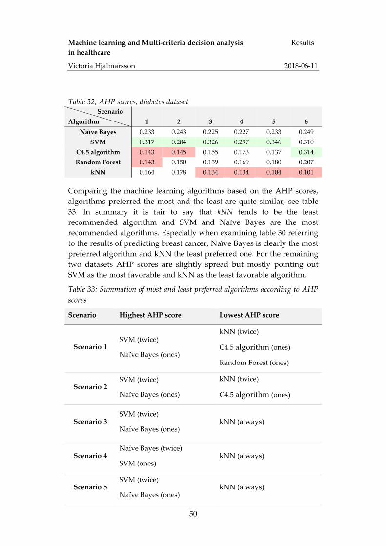
Machine learning and Multi-criteria decision analysis Results in healthcare
Victoria Hjalmarsson 2018-06-11
50
Table 32; AHP scores, diabetes dataset Scenario Algorithm 1 2 3 4 5 6
Naïve Bayes 0.233 0.243 0.225 0.227 0.233 0.249 SVM 0.317 0.284 0.326 0.297 0.346 0.310
C4.5 algorithm 0.143 0.145 0.155 0.173 0.137 0.314 Random Forest 0.143 0.150 0.159 0.169 0.180 0.207
kNN 0.164 0.178 0.134 0.134 0.104 0.101
Comparing the machine learning algorithms based on the AHP scores, algorithms preferred the most and the least are quite similar, see table 33. In summary it is fair to say that kNN tends to be the least recommended algorithm and SVM and Naïve Bayes are the most recommended algorithms. Especially when examining table 30 referring to the results of predicting breast cancer, Naïve Bayes is clearly the most preferred algorithm and kNN the least preferred one. For the remaining two datasets AHP scores are slightly spread but mostly pointing out SVM as the most favorable and kNN as the least favorable algorithm.
Table 33: Summation of most and least preferred algorithms according to AHP scores
Scenario Highest AHP score Lowest AHP score
Scenario 1 SVM (twice)
Naïve Bayes (ones)
kNN (twice)
C4.5 algorithm (ones)
Random Forest (ones)
Scenario 2 SVM (twice)
Naïve Bayes (ones)
kNN (twice)
C4.5 algorithm (ones)
Scenario 3 SVM (twice)
Naïve Bayes (ones) kNN (always)
Scenario 4 Naïve Bayes (twice)
SVM (ones) kNN (always)
Scenario 5 SVM (twice)
Naïve Bayes (ones) kNN (always)

Machine learning and Multi-criteria decision analysis Results in healthcare
Victoria Hjalmarsson 2018-06-11
51
Scenario 6 Naïve Bayes (twice)
C4.5 algorithm (ones) kNN (always)
Scenario 7 Naïve Bayes kNN
Machine learning and Multi-criteria decision analysis Analysis
in healthcare
Victoria Hjalmarsson 2018-06-11
52
5 Analysis The goal of this study is to examine what machine learning algorithms suit clinical predictions on different disease. The purpose is to emphasize the importance of MCDA when deciding what algorithms seem more ideal than others. Next, to stress the importance of thinking about and choosing the right QMMs and performance metrics when evaluating the selected machine learning algorithms. Many researchers point out the significance of selecting appropriate QMMs related to the particular scope of interest when validating machine learning algorithm (Lavesson et al. 2008; 2014; Ali, Lee & Chung 2017). In this case medical diagnosis is the defined scope. A drawback of this study is the process of selecting QMMs. Several studies, among them Ali, Lee & Chung (2017) and Lavesson et al. (2014), select QMMs by including a group of experts who discuss and rate all QMMs and from that determine which ones to include during the MCDA. In this case, QMMs are chosen based on previous research in the field of machine learning and healthcare. From that, common performance measures are evaluated and either included or excluded. However, seven scenarios are considered for the weighting processes of criteria which evens out the fact of excluding an expert group.
Comparing table 23 presenting the best and worst performing algorithms in Weka with table 33 presenting the highest and lowest AHP scores for each scenario, it is clear that there is some correlation between these results. In the majority of times (12 out of 21) SMV is the best performing algorithm, followed by Naïve Bayes (7 times), and Random Forest and C4.5 algorithm performed the best twice and ones respectively. From table 33 it is read that SVM is recommend 9 times, Naïve Bayes 8 times and C4.5 algorithm ones.
C4.5 is favored when AUC is included in the AHP evaluation. The interesting fact is that Random Forest performed the best twice on this criterion and C4.5 algorithm only denoted an overall average performance in Weka and yet, C4.5 is the favored algorithm according to AHP. This confirms the statement from, amongst others, Triantaphyllou (2000) that MCDA affects the overall outcome of what alternatives are more preferred than others, and that MCDA is significant when comparing different machine learning algorithms with each other. The factor that makes C4.5 preferred in this case, is foremost its interpretability advantages compared to the other algorithms which is an important criterion for clinical diagnosis since doctors need to

Machine learning and Multi-criteria decision analysis Analysis
in healthcare
Victoria Hjalmarsson 2018-06-11
53
understand the algorithms reasoning, especially in the case of different opinions. When comparing at what time Naïve Bayes is preferred over SVM in the AHP analysis no clear answer is determined. As in the case of C 4.5 the factor of interpretability may be crucial since Naïve Bayes is easier to follow than SVM. When examining tables 21 and 22 together with tables 31 and 32 it is clear that Naïve Bayes does not need to outperform SVM in Weka in order to achieve a higher AHP score. This also confirms the theory of no single performance metric is superior to others (Lavesson et al. 2008; 2014). This statement is further strengthened by the remark of Ali, Lee & Chung (2017) declaring the importance of including the right QMMs by inspecting the mammographic masses dataset further and the performance scores of the AUC. For the cancer dataset, Naïve Bayes and SVM which are assigned the highest AHP scores both perform the worst at several performance outputs in Weka. But, looking at the overall performance including the different QMMs they are still the best suited machine learning algorithms, which matches results from several different studies that compared different machine learning algorithms with each other (Horng et al. 2017; Alzahani et al. 2014). Another interesting observation is that SVM is outperformed in each dataset regarding the AUC score. AUC is frequently used evaluation metric in previous studies either combined with other metrics or as a single evaluation metric. If AUC would have been the only criteria in this study SVM would have been the least recommended algorithm.
For the mammographic masses dataset, the algorithms are compared to the performance of a physician on the criteria sensitivity, specificity, PPV, NPV and interpretability. The AHP score for the physician is higher than the scores of all algorithms but Naïve Bayes which outperforms all. Compared to the Weka results a physician achieves the lowest sensitivity and PPV results compared to all machine learning algorithms and outperforms all algorithms on specificity and NPV. Further it is assigned, together with C4.5 algorithm, the highest interpretability score. A physician’s prediction abilities include only extreme values similar to Naïve Bayes and SVM and therefore is seems reasonable that a physician’s AHP score lies between the scores of these two algorithms. On the other hand, from an ethical point of view it is questionable if results from the machine learning models are sufficient enough as a diagnostics support tool for breast cancer since the machine learning models underperform on specificity and NPV and only Naïve Bayes received a higher AHP score compared to the performance of a

Machine learning and Multi-criteria decision analysis Analysis
in healthcare
Victoria Hjalmarsson 2018-06-11
54
physician. The fact the all algorithms outperform a physician on sensitivity and PPV strengthens the idea of integrating machine learning as a diagnostics tool. However, to make a correct decision more information and research is necessary. It is of value to determine the optimal trade-off between different metrics. Further, it is of interest to determine whether the algorithms and a physician misclassify the same patients or different ones. If different patients are misclassified, then the machine learning algorithms can be an actual clinical support contributing to a more efficient healthcare.
For the mammographic masses dataset, the AHP scores always point out Naïve Bayes to be the most ideal and kNN as the least preferred algorithm which indicates some sort of consistency in the evaluation. This is strengthened by the other datasets as well and by table 34 where kNN is mostly assigned the lowest AHP scores and SVM and Naïve Bayes usually the highest AHP scores. This means that, no matter how weights are varied the same results are obtained. However, this can also suggest that there are one or more important factors missing.
Another limitation of this study is the risk of possible overfitting; machine learning predictions are based on associations without studying fundamental theory. The datasets that are used during this study only include 916, 270 and 768 instances for the mammographic masses, heart-statlog and the diabetes dataset respectively. Further, the diabetes dataset is relatively unbalances. These factors may negatively influence the performance results extracted from Weka, such that that the outcome possibly does not reflect reality accurately.
It is recommended to repeat this study in the presence of an expert group including both physicians and experts in machine learning and decision analysis in order to review the selected QMMs and the weighting process and also use updated and self-collected datasets.
5.1 Ethical and social aspects Methods such as machine learning to detect diseases and determine diagnoses entail some critical aspects regarding ethics. The use of patients’ data can affect the integrity of patients. Therefore, it is important to consider the circumstances at which machine learning could violate patient’s privacy and how generated information about patients could be misused. It is important to have a written ethics approval and consent before starting the study. Further, patient’s journals need to be encrypted so that no personal details are exposed.

Machine learning and Multi-criteria decision analysis Analysis
in healthcare
Victoria Hjalmarsson 2018-06-11
55
For this study three datasets available online from reliable sources where included. The datasets were already encrypted and no personal information about any patient was revealed.
Additionally, is not to forget; where physicians rely on knowledge and experience, a machine learning model relies on historic data. For a machine it is quite difficult to make accurate predictions based on new and unseen data. Since the practice of medicine is continually evolving regarding new technology and social phenomena a doctors’ knowledge and experience is very valuable for medical diagnosis. For this reason, it is important to emphasize that a doctor can never be replaced by a machine, however the machine may be an efficient compliment which can improve diagnostics and reduce time to treatment, stress among medical staff and several resource costs.
Machine learning and Multi-criteria decision analysis Conclusion in healthcare
Victoria Hjalmarsson 2018-06-11
56
6 Conclusion The overall goal of this thesis was to stress the need for a thorough MCDA in relation to machine learning evaluation. The purpose was to evaluate the value of five different machine learning algorithms as a diagnostic decision support for physicians and determine which algorithms are more suitable than others as medical support.
The five machine learning algorithms that have been examined are C4.5, Random Forest, Naïve Bayes, SVM and kNN. First all algorithms were applied on three medical datasets; the mammographic masses dataset, heart-statlog dataset and diabetes dataset. The machine learning algorithms were executed in Weka because this is a popular data mining software and well suited to compare different machine learning algorithms. The algorithms were compared on eight performance metrics; sensitivity, specificity, PPV, NPV, Kappa value, interpretability, accuracy and AUC. Next, a MCDA in term of AHP was established. The performance metrics were integrated as criteria and the five different machine learning algorithms as different alternatives. Further, a sensitivity analysis was integrated in the AHP by including seven scenarios, in which weights for the criteria were varied in order to determine what factors influence the overall preference amongst machine learning algorithms.
The study has been conducted with great care to fulfill its purpose by answering the original research questions that lead to the following results:
What machine learning algorithms are suitable to support medical diagnosis? From table 33 which summarizes the results from the AHP analysis it is clear that Naïve Bayes and SVM are recommended as suitable diagnostics support to medical staff. kNN leans to be the least preferred algorithm and therefore not recommended as a clinical decision support.
How do different evaluation criteria affect the recommendation of appropriate algorithms? When examining results from both Weka and the AHP analysis it becomes clear that there are some correlation between the algorithm’s predictive performance and the AHP score. However, algorithms performing the best do not necessarily achieve the highest AHP scores. This because multiple criteria are taken into account at once in order to

Machine learning and Multi-criteria decision analysis Conclusion in healthcare
Victoria Hjalmarsson 2018-06-11
57
optimize the decision regarding its medical tasks. Therefore, the weighting process of the criteria is an important step which need a thorough discussion among experts. This to make sure the right criteria are being evaluated and prioritized. One example of how this is crucial is shown by scenario 6 where the criteria interpretability was replaced by the frequently used metric AUC. According to the Weka performance results SMV was outperformed by all remaining algorithms indicating it would not be a suitable algorithm in the case of a single criteria evaluation. Yet, SVM was assigned the second highest AHP. Another example is verifying the significance of both the weighting process and inclusion of multiple criteria, is the comparison between the machine learning algorithms and the diagnostics statistical evaluation of a physician. The physician outperformed the machine learning algorithms on specificity, NPV and interpretability and received lower performances than all algorithms on sensitivity and PPV, which according to the weights are more important than the other criteria. Yet, the physician was assigned the second highest AHP; a lower score than Naïve Bayes and a better one than SVM. For this reason, it is confirmed that no evaluation metric is superior to all others. Nevertheless, depending on the setting and prediction task some metrics are more important than others. In the context of medical diagnostics QMMs including sensitivity, specificity, PPV, NPV and interpretability where considered more important than other typical evaluation metrics like error rate or training and testing time.
There are several directions for future work: First, to repeat this study in the presence of an expert group including both physicians and experts in machine learning and decision analysis in order to review the selected QMMs and the weighting process. Second, to repeat this study and use up to date and self-collected datasets. Third, compare the AHP scores with other MCDA methods, for example with the TOPSIS method or combine methods to identify similarities and differences in preference of machine learning algorithms. Fourth, to compare the machine learning results with results from medical staff who have diagnosed the same patients in order to examine similarities and differences in classifications. It is of interest to determine whether the machine learning model and medical staff misclassify the same patients or different ones. This could help decision makers to adjust criteria and to increase the benefits of implementing machine learning into the process of diagnostics by trying to decrease errors made by both physicians and by the machine by bringing out the best from both.

Machine learning and Multi-criteria decision analysis Reference in healthcare
Victoria Hjalmarsson 2018-06-11
58
Reference Ali, Rahman; Lee, Sungyoung, & Chung, C. Tae. 2017. Accurate multi-criteria decision making methodology for recommending machine learning algorithm. Expert Systems With Applicatins 71: 257-278. Doi: https://doi.org/10.1016/j.eswa.2016.11.034
Alzahani, Salha M. et al. 2014. An overview of data mining techniques applied for heart disease diagnostics and prediction. Lecture notes on Information Theory 2(4). Doi: 10.12720/lnit.2.4.310-315
Beheshti, Iman, Demirel, Hasan and Matsuda, Hiroshi. 2017. Classification of Alzheimer's disease and prediction of mild cognitive impairment-to-Alzheimer's conversion from structural magnetic resource imaging using feature ranking and a genetic algorithm. Computers in Biology and Medicine 83: 109-119. Doi: https://doi.org/10.1016/j.compbiomed.2017.02.011
Björklund, Maria & Paulsson, Ulf. 2012. Seminarieboken: att skriva, presentera och opponera. 2nd edition. Studentlitteratur, Lund.
Bouckaert, Remco R. et al. 2010. WEKA – Experiences with java open-source project. Journal of Machine Learning Research 11: 2533-2541.
Bramer, Max. 2016. Principles of Data Mining. 3rd edition. Springer Verlag.
Brause, Rüdiger, W. 2001. Medical Analysis and Diagnosis by Neural Networks. Crespo J., Maojo V., Martin F. (eds) Medical Data Analysis. ISMDA 2001. Lecture Notes in Computer Science 2199. Springer, Berlin, Heidelberg
Brink, Henrik; Richards, Joseph W. & Fetherolf, Mark. 2017. Real-World Machine Learining. Manning Publications, New York.
Brunnelli, M. 2015. Introduction to the Analytic Hierarchy Process. Springer Verlag, Berlin.
Chang, Chun-Lang & Chen, Chih-Hoa. 2009. Applying decision tree and neural network to increase quality of dermatologic diagnosis. Expert Systems with Applications 36(2): 4035-4041.
Chen, H. Jonathan & Ash, M. Steven. 2017. Machine Learning in Prediction in Medicine – Beyond the Peak of Inflated Expectations. The

Machine learning and Multi-criteria decision analysis Reference in healthcare
Victoria Hjalmarsson 2018-06-11
59
New England Journal of Medicine 376(26): 2507-2509. Doi: 10.1056/NEJMp1702071
Cortes, Corinna & Vapnik, Vladimir. 1995. Support-Vector Networks. Machine Learning 20(3): 273-297.
Creswell, W. John. 2003. Research Design Qualitative, Quantitative, and Mixed Methods Approaches. 2nd edition. London: Sage Publications, Inc.
Dagliati, Arianna et al. 2018. Machine Learning Methods Predict Diabetes Complications. Journal of Diabetes Science and Technology 12(2):295-302. Doi: 10.1177/1932296817706375
Dolan, James G. 2010. Multi-Criteria Clinical Decision Support: A Primer on the Use of Multiple-Criteria Decision-Making Methods to Promote Evidence-Based, Patient-Centered Healthcare. Patient-Patient-Centered-Outcome-Res 3(4): 229. Doi: https://doi.org/10.2165/11539470-000000000-00000
Fatima, Meherwar & Pasha, Maruf. 2017. Survey of Machine Learning Algorithms for Disease Diagnostic. Journal of Intelligent Learning Sytems and Applications 9: 1-16.’
Fawcett, Tom. 2006. An introduction to ROC analysis. Pattern Recognition Letters 27(8): 861-874.
Fayyad, Usama; Piatetsky-Shapiro, Greogory & Smyth, Padhraic. 1996. From data mining to knowledge discovery in databases. AI Magazine 17(3):37-54.
Fishburn, Peter. C. 1967. Additive Utilities with Incomplete Sets: Application to Priorities and Assignments. Operations Research 15(3): 537-542.
Guyon, Isabelle et al. 2002. Gene Selection for Cancer Classificatin using Support Vector Machines. Machine learning 46(1-3): 389-422.
Han, Jiawei; Kamber, Micheline & Pei, Jian. 2012. Data Mining: Concepts and Techniques. 3rd edition. San Francisco: Morgan Kaufmann Publisher.
Horng, Steven et al. 2017. Creating an automated trigger for sepsis clinical decision support at emergency department triage using machine learning. PLOS ONE 12(4). doi: e0174708.

Machine learning and Multi-criteria decision analysis Reference in healthcare
Victoria Hjalmarsson 2018-06-11
60
Hussain, L. et al. 2018. Prostate cancer detection using machine learning techniques by employing combination of feature extracting strategies. Cancer Biomark 21(2): 393-413. Doi: 10.3233/CBM-170643.
Ishizaka, A. & Nemery, P. 2013. Multi-criteria decision analysis: Methods and software. John Wiley and Sons, West Sussex, UK.
Jadoon M. Mohin et al. 2017. Classification of mammograms for breast cancer detection based on curvelet transform and multi-layer perceptron. Biomedical research 28(10): 4311- 4315.
Japkowicz, Nathalie & Shah, Mohak. 2011. Evaluating Learning Al- gorithms: A Classification Perspective. Cambridge University Press; USA.
Jian, Anju. 2015. Machine learning techniques for medical diagnosis: a review. 2nd International Conference on Science, Technology and Management, New Delhi, India.
Jongkreangkrai, C. et al. 2016. Computer-aided classification of Alzheimer’s disease based on support vector machine with combination of cerebral image features in MRI. Journal of Physics: Conference Series 694.
Kartal Hanan et al. 2016. An integrated analytic decision framework of machine learning with multi-criteria decision making for multi-attribute inventory classification. Computers & Industrial Engineering 101: 599-613.
Khanmohammadi, Sina & Rezaeiahari, Mandana. 2014. AHP based classification algorithm selection for clinical decision support system development. Procedia Computer Science 36: 328-334.
Lavesson, Niklas & Davidsson, Paul. 2008. Generic Methods for Multi-criteria Evaluation. SIAM International Conference in data mining, Atlanta, Georgia.
Lavesson, Niklas et al. 2014. A method for evaluation of learning components. Automated Software Engineering 21(1): 41-63. Doi: https://doi.org/10.1007/s10515-013-0123-1
Li, Qingshan; Zhang, Lihang & Chu, Hua. 2012. An AHP-Based Assessment Model for Clinical Diagnosis and Decision. Artificial

Machine learning and Multi-criteria decision analysis Reference in healthcare
Victoria Hjalmarsson 2018-06-11
61
Intelligence and Computational Intelligence. Lecture notes in Computer Science 7530. Springer, Berlin, Heidelberg.
Ludvigsson, Jonas F. & Ekbom, Anders. 2017. Medicink statistik – diagnostiska tester. Internetmedicin AB. Doi: https://www.internetmedicin.se/page.aspx?id=3282
Machine Learning Group at the University of Waikato. 2018. Weka 3: Data mining software in Java. https://www.cs.waikato.ac.nz/ml/weka/ (Viewed: 2018-01-12)
Marsh, Kevin et al. 2017. Multi-Criteria Decision Analysis to Support Healthcare Decisions. Springer International Publishing. eBook.
McKinsey, (2016). Värdet av digital teknik i den svenska vården. McKinsey & Company.
Mu, Enrique & Pereyra-Rojas, Milagros. 2017. Practical Decision Making. Springer International Publishing.
OpenML. 2018. Heart-statlog. https://www.openml.org/d/53 (Viewed 2018-03-07)
Othman bin, Mohd F. & Yau, Thomas M. S. 2007. Comparison of Different Classification Techniques Using WEKA for Breast Cancer. 3rd Kuala Lumpur International Conference on Biomedical Engineering 2006. Proceeding. Part of the IFMBE Proceedings, vol. 15. Springer, Berlin, Heidelberg.
Rahimi, Shahram; Gandy, Lisa & Mogharreban, Namdar. 2007. A Web-based High-Performance Multicriteria Decision Support System for Medical Diagnosis. International Journal of Intelligent Systems. 22: 1083–1099. Doi: 10.1002/int.20238
Ranganatha, S. et al. 2013. Medical data mining and analysis for heart disease dataset using classification techniques. National Conference on Challenges in Research & Technology in the Coming Decades.
Saaty, Thomas L. 1977. A scaling method for priorities in hierarchical structures. Journal of Mathematical Psychology. 15(3): 234-281. Doi: https://doi.org/10.1016/0022-2496(77)90033-5

Machine learning and Multi-criteria decision analysis Reference in healthcare
Victoria Hjalmarsson 2018-06-11
62
Saaty, Thomas L. 2012. Decision Making for Leaders: The Analytic Hierarchy Process for Decisions in a Complex World. 3rd Edition. Pittsburgh: RWS Publications.
Schmidt, Katharia et al. 2015. Applying the Analytical Hierarchy Process in healthcare research: A systematic literature review and evaluation of reporting. BMC Medical Informatics & Decision Making 15:112.
Smith, Megan, Higgs, Joy & Ellis, Elizabeth. 2008. Factors influencing clinical decision making. 3rd ed. Butterworth Heinemann Elsevier, pp 89 -100.
Soni, Jyoti et al. 2011. Predictive Data Mining for Medical Diagnosis: An Overview of Heart Disease Prediction. Internatinal Journal of Computer Applications 17(8): 43-48.
Supino, Phyllis G. & Borer, Jeffery S. 2012. Principles of Research Methodology. Springer Verlag: New York.
Statens Beredning för Medicinsk och Social Utvärdering (SBU). 2014. Statistiska begrepp i medicinsk utvärderingar. Bilagadel.
Schüür, Friederike. 2017. Why your relationship is likely to last (or not): using local interpretable Model – Agnostic Explanation. Cloudera Fast Forward Labs. [Blog]. 1st September. http://blog.fastforwardlabs.com/2017/09/01/LIME-for-couples.html (Viewed 2018-04-20)
Schervish, Mark J. 1995. Theory of Statistics. Springer-Verlag, New York.
Segaran, Toby. 2007. Programming Collective Intelligence. O’Reilly Media, Sebastopol
Shouman, Mai; Turner, Tim & Stocker, Rob. 2012. Applying k-Nearest Neighbor in Diagnosing Heart Disease Patients. International Journal of Information and Education Technology 2(3).
Soares, Carlos; Costa, J. & Brazdil, Pavel B. 2000. A simple and intuitive measure for multi-criteria evaluation of classification algorithms. In ECML2000 Workshop on Meta-Learning: Building Automatic Advice Strategies for Model Selection and Method Combination, 87– 96. 2000, Barcelona. Springer Science.

Machine learning and Multi-criteria decision analysis Reference in healthcare
Victoria Hjalmarsson 2018-06-11
63
Socialstyrelsen. 2014. Screening för bröstcancer.
Solanki, Ashokkumar V. 2014. Data Mining Techniques Using Weka classification for Sickle Cell Disease. International Journal of Computer Science and Information Technologies 5(4): 5857-5860.
Thakkar, Kunal et al. 2016. AHP and Machine Learning Techniques for Wine Recommendation. International Journal of Computer Science and Information Technologies 7(5): 2349-2352.
Triantaphyllou, Evangelos. 2000. Multi-criteria decision making methods: A comparative study. Dordrecht: Kluwer Academic Publishers.
UCI Machine Learning Repository. 2018. Mammographic Mass Data Set. http://archive.ics.uci.edu/ml/datasets/Mammographic+Mass (Viewed 2018-03-07)
Vaidya, O.S. & Kumar, S. 2004. Analytic hierarchy process: an overview of applications. European Journal of Operational Research 169(1), 1–29.
Vapnik, Vladimir. 1998. Statistical learning theory. John Wiley & Sons, New Jersey.
Wiharto, Wiharto; Kusnanto, Hari; Herianto, Herianto. 2016. Interpretation of Clinical Data Based on C4.5 Algorithm for the Diagnosis of Colonary Heart Disease. Healthcare Informatics Research 22(3): 186-195.
Witten, H. Ian; Frank, Eibe & Hall A. Mark. 2011. Data Mining Practical Machine Learning Tools and Techniques. 3rd edition. Morgan Kaufman, San Francisco.
Wu, Xindong et al. 2008. Top 10 algorithms in data mining. Knowledge and Information Systems. 14(1):1-37. Doi: https://doi.org/10.1007/s10115-007-0114-2 (Viewed 2018-02-19)
Xu, Weifeng et al. 2017. Risk prediction of type II diabetes based on random forest model. IEEE Conference, India. Doi: 10.1109/AEEICB.2017.7972337
Zeshui, X. & Cuiping, W. 1999. A consistency improving method in the analytic hierarchy process. European Journal of Operational Research 116: 443–449.

Machine learning and Multi-criteria decision analysis Reference in healthcare
Victoria Hjalmarsson 2018-06-11
64
Zhao, Jitao & Wang, Ting. 2010. A general framework for medical data mining. Future Information Technology and Management Engineering, 2010 International IEEE Conference, Changzhou, China.
Machine learning and Multi-criteria decision analysis Appendix A – AHP in healthcare
Victoria Hjalmarsson 2018-06-11
65
Appendix A – AHP This section presents results extracted from excel for step 4 explained in section 2.2.2 addressing the AHP method.
For the pairwise comparison of the five machine learning algorithms an interval is defined corresponding to Saaty’s scale of comparison. This, to ensure that the comparisons are consistent and depending on the performance results extracted from Weka. The interval reflects the difference between the same criteria of two different algorithms. For example, if PPV equal 0.5 for SVM and 0.2 for kNN, then the difference 0.3 indicates that SVM is ‘moderate more important’ than kNN according to table 34.
Table 34: Saaty's scale of comparison including a specified intervals
Saaty’s scale of comparison
Intensity Definition Intervals
1 Equal importance ≤ 0.020
3 Moderate more important 0.021-0.040
5 Strongly more important 0.041-0.060
7 Very strongly more important 0.061 -0.080
9 Extremely important 0.081 ≤
For each criteria a pairwise comparison matrix of alternatives, hence the five machine learning algorithms need to be established. Thus, for each dataset eight comparison matrices are generated. Tables 35 – 55 present the pairwise comparison of alternatives and the corresponding normalized comparison matrices for the mammographic masses; tables 56 – 71 represent the heart-statlog dataset and tables 72 – 87 the diabetes dataset.
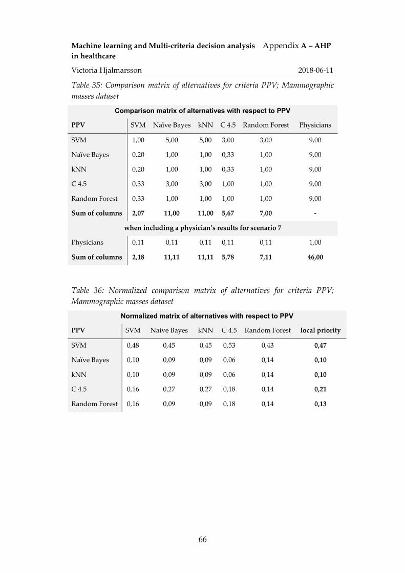
Machine learning and Multi-criteria decision analysis Appendix A – AHP in healthcare
Victoria Hjalmarsson 2018-06-11
66
Table 35: Comparison matrix of alternatives for criteria PPV; Mammographic masses dataset
Comparison matrix of alternatives with respect to PPV
PPV SVM Naïve Bayes kNN C 4.5 Random Forest Physicians
SVM 1,00 5,00 5,00 3,00 3,00 9,00
Naïve Bayes 0,20 1,00 1,00 0,33 1,00 9,00
kNN 0,20 1,00 1,00 0,33 1,00 9,00
C 4.5 0,33 3,00 3,00 1,00 1,00 9,00
Random Forest 0,33 1,00 1,00 1,00 1,00 9,00
Sum of columns 2,07 11,00 11,00 5,67 7,00 -
when including a physician’s results for scenario 7
Physicians 0,11 0,11 0,11 0,11 0,11 1,00
Sum of columns 2,18 11,11 11,11 5,78 7,11 46,00
Table 36: Normalized comparison matrix of alternatives for criteria PPV; Mammographic masses dataset
Normalized matrix of alternatives with respect to PPV
PPV SVM Naive Bayes kNN C 4.5 Random Forest local priority
SVM 0,48 0,45 0,45 0,53 0,43 0,47
Naïve Bayes 0,10 0,09 0,09 0,06 0,14 0,10
kNN 0,10 0,09 0,09 0,06 0,14 0,10
C 4.5 0,16 0,27 0,27 0,18 0,14 0,21
Random Forest 0,16 0,09 0,09 0,18 0,14 0,13

Machine learning and Multi-criteria decision analysis Appendix A – AHP in healthcare
Victoria Hjalmarsson 2018-06-11
67
Table 37: Normalized comparison matrix of alternatives for criteria PPV; scenario 7; Mammographic masses dataset
Normalized matrix of alternatives with respect to PPV; scenario 7
PPV SVM Naive Bayes kNN C 4.5 Random Forest Physicians local priority
SVM 0,46 0,45 0,45 0,52 0,42 0,20 0,42
Naïve Bayes 0,09 0,09 0,09 0,06 0,14 0,20 0,11
KNN 0,09 0,09 0,09 0,06 0,14 0,20 0,11
C 4.5 0,15 0,27 0,27 0,17 0,14 0,20 0,20
Random Forest 0,15 0,09 0,09 0,17 0,14 0,20 0,14
Physicians 0,05 0,01 0,01 0,02 0,02 0,02 0,02
Table 38: Comparison matrix of alternatives for criteria NPV; Mammographic masses dataset
Comparison matrix of alternatives with respect to NPV
NPV SVM Naïve Bayes kNN C 4.5 Random Forest Physician
SVM 1,00 0,20 1,00 0,33 0,33 0.11
Naïve Bayes 5,00 1,00 5,00 3,00 3,00 0.11
kNN 1,00 0,20 1,00 0,33 0,33 0.11
C 4.5 3,00 0,33 3,00 1,00 1,00 0.11
Random Forest 3,00 0,33 3,00 1,00 1,00 0.11
Sum of columns 13,00 2,07 13,00 5,67 5,67 -
when including a physician’s results for scenario 7
Physicians 9.00 9.00 9.00 9.00 9.00 1.00
Sum of columns 22.00 11.07 22.00 14.67 14.67 1.56

Machine learning and Multi-criteria decision analysis Appendix A – AHP in healthcare
Victoria Hjalmarsson 2018-06-11
68
Table 39: Normalized comparison matrix of alternatives for criteria NPV; Mammographic masses dataset
Normalized matrix of alternatives with respect to NPV
NPV SVM Naïve Bayes kNN C 4.5 Random Forest local priority
SVM 0,08 0,10 0,08 0,06 0,06 0,07
Naïve Bayes 0,38 0,48 0,38 0,53 0,53 0,46
kNN 0,08 0,10 0,08 0,06 0,06 0,07
C 4.5 0,23 0,16 0,23 0,18 0,18 0,20
Random Forest 0,23 0,16 0,23 0,18 0,18 0,20
Table 40: Normalized comparison matrix of alternatives for criteria NPV; scenario 7; Mammographic masses dataset
Normalized matrix of alternatives with respect to NPV; scenario 7
NPV SVM Naive Bayes kNN C 4.5 Random Forest Physicians local priority
SVM 0,05 0,02 0,05 0,02 0,02 0,07 0,04
Naïve Bayes 0,23 0,09 0,23 0,20 0,20 0,07 0,17
kNN 0,05 0,02 0,05 0,02 0,02 0,07 0,04
C 4.5 0,14 0,03 0,14 0,07 0,07 0,07 0,09
Random Forest 0,14 0,03 0,14 0,07 0,07 0,07 0,09
Physicians 0,41 0,81 0,41 0,61 0,61 0,64 0,58
Table 41: Comparison matrix of alternatives for criteria Interpretability; Mammographic masses dataset
Comparison matrix of alternatives with respect to Interpretability
Interpretability SVM Naïve Bayes kNN C 4.5 Random Forest Physician
SVM 1,00 0,33 0,25 0,20 0,50 0.20
Naïve Bayes 3,00 1,00 0,50 0,33 2,00 0.50
KNN 4,00 2,00 1,00 0,50 3,00 0.33
C 4.5 5,00 3,00 2,00 1,00 4,00 1.00
Random Forest 2,00 0,50 0,33 0,25 1,00 0.25
Sum of columns 15,00 6,83 4,08 2,28 10,50 -
when including a physician’s results for scenario 7
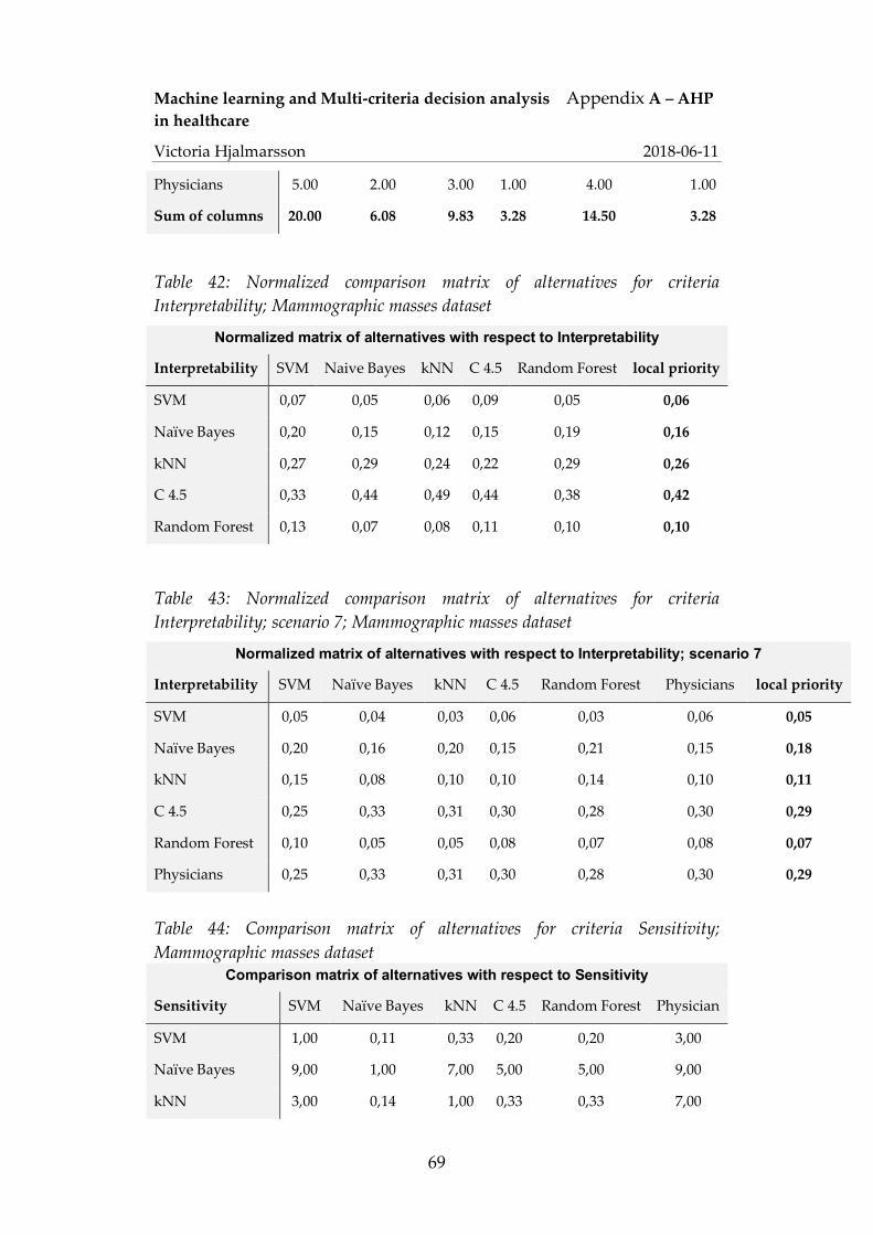
Machine learning and Multi-criteria decision analysis Appendix A – AHP in healthcare
Victoria Hjalmarsson 2018-06-11
69
Physicians 5.00 2.00 3.00 1.00 4.00 1.00
Sum of columns 20.00 6.08 9.83 3.28 14.50 3.28
Table 42: Normalized comparison matrix of alternatives for criteria Interpretability; Mammographic masses dataset
Normalized matrix of alternatives with respect to Interpretability
Interpretability SVM Naive Bayes kNN C 4.5 Random Forest local priority
SVM 0,07 0,05 0,06 0,09 0,05 0,06
Naïve Bayes 0,20 0,15 0,12 0,15 0,19 0,16
kNN 0,27 0,29 0,24 0,22 0,29 0,26
C 4.5 0,33 0,44 0,49 0,44 0,38 0,42
Random Forest 0,13 0,07 0,08 0,11 0,10 0,10
Table 43: Normalized comparison matrix of alternatives for criteria Interpretability; scenario 7; Mammographic masses dataset
Normalized matrix of alternatives with respect to Interpretability; scenario 7
Interpretability SVM Naïve Bayes kNN C 4.5 Random Forest Physicians local priority
SVM 0,05 0,04 0,03 0,06 0,03 0,06 0,05
Naïve Bayes 0,20 0,16 0,20 0,15 0,21 0,15 0,18
kNN 0,15 0,08 0,10 0,10 0,14 0,10 0,11
C 4.5 0,25 0,33 0,31 0,30 0,28 0,30 0,29
Random Forest 0,10 0,05 0,05 0,08 0,07 0,08 0,07
Physicians 0,25 0,33 0,31 0,30 0,28 0,30 0,29
Table 44: Comparison matrix of alternatives for criteria Sensitivity; Mammographic masses dataset
Comparison matrix of alternatives with respect to Sensitivity
Sensitivity SVM Naïve Bayes kNN C 4.5 Random Forest Physician
SVM 1,00 0,11 0,33 0,20 0,20 3,00
Naïve Bayes 9,00 1,00 7,00 5,00 5,00 9,00
kNN 3,00 0,14 1,00 0,33 0,33 7,00

Machine learning and Multi-criteria decision analysis Appendix A – AHP in healthcare
Victoria Hjalmarsson 2018-06-11
70
C 4.5 5,00 0,20 3,00 1,00 1,00 9,00
Random Forest 5,00 0,20 3,00 1,00 1,00 9,00
Sum of columns 23.00 1.65 14.33 7.53 7.53 -
when including a physician’s results for scenario 7
Physician 0,33 0,11 0,14 0,11 0,11 1,00
Sum of columns 23,33 1,77 14,48 7,64 7,64 38,00
Table 45: Normalized comparison matrix of alternatives for criteria Sensitivity; Mammographic masses dataset
Normalized matrix of alternatives with respect to Sensitivity
Sensitivity SVM Naive Bayes KNN C 4.5 Random Forest local priority
SVM 0,04 0,07 0,02 0,03 0,03 0,04
Naïve Bayes 0,39 0,60 0,49 0,66 0,66 0,56
KNN 0,13 0,09 0,07 0,04 0,04 0,08
C 4.5 0,22 0,12 0,21 0,13 0,13 0,16
Random Forest 0,22 0,12 0,21 0,13 0,13 0,16
Table 46: Normalized comparison matrix of alternatives for criteria Sensitivity; scenario 7; Mammographic masses dataset
Normalized matrix of alternatives with respect to Sensitivity; scenario 7
Sensitivity SVM Naïve Bayes kNN C 4.5 Random Forest Physician local priority
SVM 0,04 0,06 0,02 0,03 0,03 0,08 0,04
Naïve Bayes 0,39 0,57 0,48 0,65 0,65 0,24 0,50
kNN 0,13 0,08 0,07 0,04 0,04 0,18 0,09
C 4.5 0,21 0,11 0,21 0,13 0,13 0,24 0,17
Random Forest 0,21 0,11 0,21 0,13 0,13 0,24 0,17
Physician 0,01 0,06 0,01 0,01 0,01 0,03 0,02

Machine learning and Multi-criteria decision analysis Appendix A – AHP in healthcare
Victoria Hjalmarsson 2018-06-11
71
Table 47: Comparison matrix of alternatives for criteria Specificity; Mammographic masses dataset
Comparison matrix of alternatives with respect to Specificity
Specificity SVM Naïve Bayes kNN C 4.5 Random Forest Physicians
SVM 1,00 7,00 5,00 5,00 5,00 1,00
Naïve Bayes 0,14 1,00 0,33 0,33 0,33 0,11
kNN 0,20 3,00 1,00 1,00 1,00 0,14
C 4.5 0,20 3,00 1,00 1,00 1,00 0,20
Random Forest 0,20 3,00 1,00 1,00 1,00 0,20
Sum of columns 1.74 17.00 8.33 8.33 8.33 -
when including a physician’s results for scenario 7
Physician 1,00 9,00 7,00 5,00 5,00 1,00
Sum of columns 2,74 26,00 15,33 13,33 13,33 2,65
Table 48: Normalized comparison matrix of alternatives for criteria Specificity; Mammographic masses dataset
Normalized matrix of alternatives with respect to specificity
Specificity SVM Naïve Bayes kNN C 4.5 Random Forest local priority
SVM 0,57 0,41 0,60 0,60 0,60 0,56
Naïve Bayes 0,08 0,06 0,04 0,04 0,04 0,05
kNN 0,11 0,18 0,12 0,12 0,12 0,13
C 4.5 0,11 0,18 0,12 0,12 0,12 0,13
Random Forest 0,11 0,18 0,12 0,12 0,12 0,13

Machine learning and Multi-criteria decision analysis Appendix A – AHP in healthcare
Victoria Hjalmarsson 2018-06-11
72
Table 49: Normalized comparison matrix of alternatives for criteria Specificity; scenario 7; Mammographic masses dataset
Normalized matrix of alternatives with respect to specificity; scenario 7
Specificity SVM Naïve Bayes kNN C 4.5 Random Forest Physician local priority
SVM 0,36 0,27 0,33 0,38 0,38 0,38 0,35
Naïve Bayes 0,05 0,04 0,02 0,03 0,03 0,04 0,03
kNN 0,07 0,12 0,07 0,08 0,08 0,05 0,08
C 4.5 0,07 0,12 0,07 0,08 0,08 0,08 0,08
Random Forest 0,07 0,12 0,07 0,08 0,08 0,08 0,08
Physician 0,36 0,35 0,46 0,38 0,38 0,38 0,38
Table 50: Comparison matrix of alternatives for criteria Kappa value; Mammographic masses dataset
Comparison matrix of alternatives with respect to Kappa value
Kappa SVM Naïve Bayes kNN C 4.5 Random Forest
SVM 1,00 1,00 7,00 1,00 9,00
Naïve Bayes 1,00 1,00 9,00 1,00 9,00
kNN 0,14 0,11 1,00 0,11 1,00
C 4.5 1,00 1,00 9,00 1,00 9,00
Random Forest 0,11 0,11 1,00 0,11 1,00
Sum of columns 3,25 3,22 27,00 3,22 29,00
Table 51: Normalized comparison matrix of alternatives for criteria Kappa value; Mammographic masses dataset
Normalized matrix of alternatives with respect to Kappa value
Kappa SVM Naïve Bayes kNN C 4.5 Random Forest local priority
SVM 0,31 0,31 0,26 0,31 0,31 0,30
Naïve Bayes 0,31 0,31 0,33 0,31 0,31 0,31
kNN 0,04 0,03 0,04 0,03 0,03 0,04
C 4.5 0,31 0,31 0,33 0,31 0,31 0,31
Random Forest 0,03 0,03 0,04 0,03 0,03 0,03

Machine learning and Multi-criteria decision analysis Appendix A – AHP in healthcare
Victoria Hjalmarsson 2018-06-11
73
Table 52: Comparison matrix of alternatives for criteria Accuracy; Mammographic masses dataset
Comparison matrix of alternatives with respect to Accuracy
Accuracy SVM Naive Bayes KNN C 4.5 Random Forest
SVM 1,00 0,33 1,00 1,00 1,00
Naïve Bayes 3,00 1,00 3,00 1,00 3,00
KNN 1,00 0,33 1,00 3,00 1,00
C 4.5 1,00 1,00 0,33 1,00 1,00
Random Forest 1,00 0,33 1,00 1,00 1,00
Sum of columns 7,00 3,00 6,33 7,00 7,00
Table 53: Normalized comparison matrix of alternatives for criteria Accuracy; Mammographic masses dataset
Normalized matrix of alternatives with respect to Accuracy
Accuracy SVM Naïve Bayes kNN C 4.5 Random Forest local priority
SVM 0,14 0,11 0,16 0,14 0,14 0,14
Naïve Bayes 0,43 0,33 0,47 0,14 0,43 0,36
kNN 0,14 0,11 0,16 0,43 0,14 0,20
C 4.5 0,14 0,33 0,05 0,14 0,14 0,16
Random Forest 0,14 0,11 0,16 0,14 0,14 0,14
Table 54: Comparison matrix of alternatives for criteria AUC; Mammographic masses dataset
Comparison matrix of alternatives with respect to AUC
AUC SVM Naïve Bayes kNN C 4.5 Random Forest
SVM 1,00 0,11 0,33 0,33 0,20
Naïve Bayes 9,00 1,00 5,00 5,00 3,00
kNN 3,00 0,20 1,00 1,00 0,33
C 4.5 3,00 0,20 1,00 1,00 1,00
Random Forest 5,00 0,33 3,00 1,00 1,00
Sum of columns 21,00 1,84 10,33 8,33 5,53
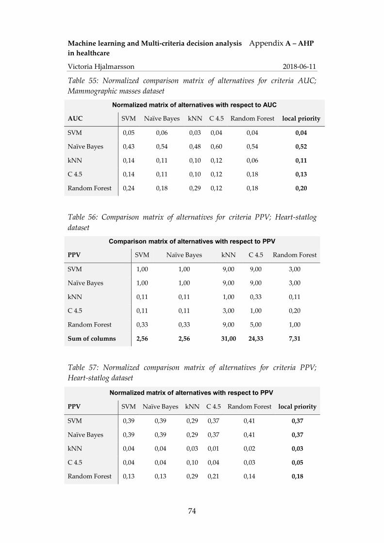
Machine learning and Multi-criteria decision analysis Appendix A – AHP in healthcare
Victoria Hjalmarsson 2018-06-11
74
Table 55: Normalized comparison matrix of alternatives for criteria AUC; Mammographic masses dataset
Normalized matrix of alternatives with respect to AUC
AUC SVM Naïve Bayes kNN C 4.5 Random Forest local priority
SVM 0,05 0,06 0,03 0,04 0,04 0,04
Naïve Bayes 0,43 0,54 0,48 0,60 0,54 0,52
kNN 0,14 0,11 0,10 0,12 0,06 0,11
C 4.5 0,14 0,11 0,10 0,12 0,18 0,13
Random Forest 0,24 0,18 0,29 0,12 0,18 0,20
Table 56: Comparison matrix of alternatives for criteria PPV; Heart-statlog dataset
Comparison matrix of alternatives with respect to PPV
PPV SVM Naïve Bayes kNN C 4.5 Random Forest
SVM 1,00 1,00 9,00 9,00 3,00
Naïve Bayes 1,00 1,00 9,00 9,00 3,00
kNN 0,11 0,11 1,00 0,33 0,11
C 4.5 0,11 0,11 3,00 1,00 0,20
Random Forest 0,33 0,33 9,00 5,00 1,00
Sum of columns 2,56 2,56 31,00 24,33 7,31
Table 57: Normalized comparison matrix of alternatives for criteria PPV; Heart-statlog dataset
Normalized matrix of alternatives with respect to PPV
PPV SVM Naïve Bayes kNN C 4.5 Random Forest local priority
SVM 0,39 0,39 0,29 0,37 0,41 0,37
Naïve Bayes 0,39 0,39 0,29 0,37 0,41 0,37
kNN 0,04 0,04 0,03 0,01 0,02 0,03
C 4.5 0,04 0,04 0,10 0,04 0,03 0,05
Random Forest 0,13 0,13 0,29 0,21 0,14 0,18

Machine learning and Multi-criteria decision analysis Appendix A – AHP in healthcare
Victoria Hjalmarsson 2018-06-11
75
Table 58: Comparison matrix of alternatives for criteria NPV; Heart-statlog dataset
Comparison matrix of alternatives with respect to NPV
NPV SVM Naïve Bayes kNN C 4.5 Random Forest
SVM 1,00 1,00 7,00 5,00 1,00
Naïve Bayes 1,00 1,00 5,00 5,00 1,00
kNN 0,14 0,20 1,00 1,00 0,20
C 4.5 0,20 0,20 1,00 1,00 0,20
Random Forest 1,00 1,00 5,00 5,00 1,00
Sum of columns 3,34 3,40 19,00 17,00 3,40
Table 59: Normalized comparison matrix of alternatives for criteria NPV; Heart-statlog dataset
Normalized matrix of alternatives with respect to NPV
NPV SVM Naïve Bayes kNN C 4.5 Random Forest local priority
SVM 0,30 0,29 0,37 0,29 0,29 0,31
Naïve Bayes 0,30 0,29 0,26 0,29 0,29 0,29
kNN 0,04 0,06 0,05 0,06 0,06 0,05
C 4.5 0,06 0,06 0,05 0,06 0,06 0,06
Random Forest 0,30 0,29 0,26 0,29 0,29 0,29
Table 60: Comparison matrix of alternatives for criteria Interpretability; Heart-statlog dataset
Comparison matrix of alternatives with respect to Interpretability
Interpretability SVM Naïve Bayes kNN C 4.5 Random Forest
SVM 1,00 0,33 0,25 0,20 0,50
Naïve Bayes 3,00 1,00 0,50 0,33 2,00
kNN 4,00 2,00 1,00 0,50 3,00
C 4.5 5,00 3,00 2,00 1,00 4,00
Random Forest 2,00 0,50 0,33 0,25 1,00
Sum of columns 15,00 6,83 4,08 2,28 10,50

Machine learning and Multi-criteria decision analysis Appendix A – AHP in healthcare
Victoria Hjalmarsson 2018-06-11
76
Table 61: Normalized comparison matrix of alternatives for criteria Interpretability; Heart-statlog dataset
Normalized matrix of alternatives with respect to Interpretability
Interpretability SVM Naïve Bayes kNN C 4.5 Random Forest local priority
SVM 0,07 0,05 0,06 0,09 0,05 0,06
Naïve Bayes 0,20 0,15 0,12 0,15 0,19 0,16
kNN 0,27 0,29 0,24 0,22 0,29 0,26
C 4.5 0,33 0,44 0,49 0,44 0,38 0,42
Random Forest 0,13 0,07 0,08 0,11 0,10 0,10
Table 62: Comparison matrix of alternatives for criteria Sensitivity; Heart-statlog dataset
Comparison matrix of alternatives with respect to sensitivity
Sensitivity SVM Naïve Bayes kNN C 4.5 Random Forest
SVM 1,00 1,00 7,00 7,00 1,00
Naïve Bayes 1,00 1,00 5,00 5,00 1,00
kNN 0,14 0,20 1,00 1,00 1,00
C 4.5 0,14 0,20 1,00 1,00 1,00
Random Forest 1,00 1,00 1,00 1,00 1,00
Sum of columns 3,29 3,40 15,00 15,00 5,00
Table 63: Normalized comparison matrix of alternatives for criteria Sensitivity; Heart-statlog dataset
Normalized matrix of alternatives with respect to Sensitivity
Sensitivity SVM Naïve Bayes kNN C 4.5 Random Forest local priority
SVM 0,30 0,29 0,47 0,47 0,20 0,35
Naïve Bayes 0,30 0,29 0,33 0,33 0,20 0,29
kNN 0,04 0,06 0,07 0,07 0,20 0,09
C 4.5 0,04 0,06 0,07 0,07 0,20 0,09
Random Forest 0,30 0,29 0,07 0,07 0,20 0,19

Machine learning and Multi-criteria decision analysis Appendix A – AHP in healthcare
Victoria Hjalmarsson 2018-06-11
77
Table 64: Comparison matrix of alternatives for criteria Specificity; Heart-statlog dataset
Comparison matrix of alternatives with respect to specificity
Specificity SVM Naïve Bayes kNN C 4.5 Random Forest
SVM 1,00 1,00 9,00 9,00 3,00
Naïve Bayes 1,00 1,00 9,00 9,00 3,00
kNN 0,11 0,11 1,00 0,33 0,14
C 4.5 0,11 0,11 3,00 1,00 0,20
Random Forest 0,33 0,33 7,00 5,00 1,00
Sum of columns 2,56 2,56 29,00 24,33 7,34
Table 65: Normalized comparison matrix of alternatives for criteria Specificity; Heart-statlog dataset
Normalized matrix of alternatives with respect to specificity
Specificity SVM Naïve Bayes kNN C 4.5 Random Forest local priority
SVM 0,39 0,39 0,31 0,37 0,41 0,37
Naïve Bayes 0,39 0,39 0,31 0,37 0,41 0,37
kNN 0,04 0,04 0,03 0,01 0,02 0,03
C 4.5 0,04 0,04 0,10 0,04 0,03 0,05
Random Forest 0,13 0,13 0,24 0,21 0,14 0,17
Table 66: Comparison matrix of alternatives for criteria Kappa value; Heart-statlog dataset
Comparison matrix of alternatives with respect to Kappa value
Kappa SVM Naïve Bayes kNN C 4.5 Random Forest
SVM 1,00 1,00 9,00 9,00 5,00
Naïve Bayes 1,00 1,00 9,00 9,00 5,00
kNN 0,11 0,11 1,00 0,33 0,11
C 4.5 0,11 0,11 3,00 1,00 0,11
Random Forest 0,20 0,20 9,00 9,00 1,00
Sum of columns 2,42 2,42 31,00 28,33 11,22
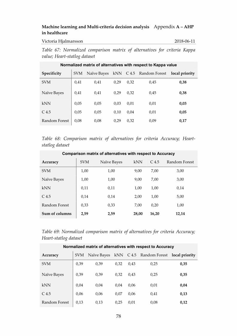
Machine learning and Multi-criteria decision analysis Appendix A – AHP in healthcare
Victoria Hjalmarsson 2018-06-11
78
Table 67: Normalized comparison matrix of alternatives for criteria Kappa value; Heart-statlog dataset
Normalized matrix of alternatives with respect to Kappa value
Specificity SVM Naïve Bayes kNN C 4.5 Random Forest local priority
SVM 0,41 0,41 0,29 0,32 0,45 0,38
Naïve Bayes 0,41 0,41 0,29 0,32 0,45 0,38
kNN 0,05 0,05 0,03 0,01 0,01 0,03
C 4.5 0,05 0,05 0,10 0,04 0,01 0,05
Random Forest 0,08 0,08 0,29 0,32 0,09 0,17
Table 68: Comparison matrix of alternatives for criteria Accuracy; Heart-statlog dataset
Comparison matrix of alternatives with respect to Accuracy
Accuracy SVM Naïve Bayes kNN C 4.5 Random Forest
SVM 1,00 1,00 9,00 7,00 3,00
Naïve Bayes 1,00 1,00 9,00 7,00 3,00
kNN 0,11 0,11 1,00 1,00 0,14
C 4.5 0,14 0,14 2,00 1,00 5,00
Random Forest 0,33 0,33 7,00 0,20 1,00
Sum of columns 2,59 2,59 28,00 16,20 12,14
Table 69: Normalized comparison matrix of alternatives for criteria Accuracy; Heart-statlog dataset
Normalized matrix of alternatives with respect to Accuracy
Accuracy SVM Naïve Bayes kNN C 4.5 Random Forest local priority
SVM 0,39 0,39 0,32 0,43 0,25 0,35
Naïve Bayes 0,39 0,39 0,32 0,43 0,25 0,35
kNN 0,04 0,04 0,04 0,06 0,01 0,04
C 4.5 0,06 0,06 0,07 0,06 0,41 0,13
Random Forest 0,13 0,13 0,25 0,01 0,08 0,12
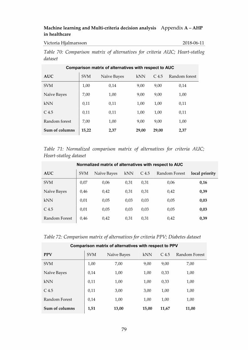
Machine learning and Multi-criteria decision analysis Appendix A – AHP in healthcare
Victoria Hjalmarsson 2018-06-11
79
Table 70: Comparison matrix of alternatives for criteria AUC; Heart-statlog dataset
Comparison matrix of alternatives with respect to AUC
AUC SVM Naïve Bayes kNN C 4.5 Random forest
SVM 1,00 0,14 9,00 9,00 0,14
Naïve Bayes 7,00 1,00 9,00 9,00 1,00
kNN 0,11 0,11 1,00 1,00 0,11
C 4.5 0,11 0,11 1,00 1,00 0,11
Random forest 7,00 1,00 9,00 9,00 1,00
Sum of columns 15,22 2,37 29,00 29,00 2,37
Table 71: Normalized comparison matrix of alternatives for criteria AUC; Heart-statlog dataset
Normalized matrix of alternatives with respect to AUC
AUC SVM Naïve Bayes kNN C 4.5 Random Forest local priority
SVM 0,07 0,06 0,31 0,31 0,06 0,16
Naïve Bayes 0,46 0,42 0,31 0,31 0,42 0,39
kNN 0,01 0,05 0,03 0,03 0,05 0,03
C 4.5 0,01 0,05 0,03 0,03 0,05 0,03
Random Forest 0,46 0,42 0,31 0,31 0,42 0,39
Table 72: Comparison matrix of alternatives for criteria PPV; Diabetes dataset
Comparison matrix of alternatives with respect to PPV
PPV SVM Naïve Bayes kNN C 4.5 Random Forest
SVM 1,00 7,00 9,00 9,00 7,00
Naïve Bayes 0,14 1,00 1,00 0,33 1,00
kNN 0,11 1,00 1,00 0,33 1,00
C 4.5 0,11 3,00 3,00 1,00 1,00
Random Forest 0,14 1,00 1,00 1,00 1,00
Sum of columns 1,51 13,00 15,00 11,67 11,00

Machine learning and Multi-criteria decision analysis Appendix A – AHP in healthcare
Victoria Hjalmarsson 2018-06-11
80
Table 73: Normalized comparison matrix of alternatives for criteria PPV; Diabetes dataset
Normalized matrix of alternatives with respect to PPV
PPV SVM Naïve Bayes kNN C 4.5 Random Forest local priority
SVM 0,66 0,54 0,60 0,77 0,64 0,64
Naïve Bayes 0,09 0,08 0,07 0,03 0,09 0,07
kNN 0,07 0,08 0,07 0,03 0,09 0,07
C 4.5 0,07 0,23 0,20 0,09 0,09 0,14
Random Forest 0,09 0,08 0,07 0,09 0,09 0,08
Table 74: Comparison matrix of alternatives for criteria NPV; Diabetes dataset
Comparison matrix of alternatives with respect to NPV
NPV SVM Naïve Bayes kNN C 4.5 Random Forest
SVM 1,00 1,00 3,00 1,00 1,00
Naïve Bayes 1,00 1,00 5,00 1,00 1,00
kNN 0,33 0,20 1,00 0,33 0,20
C 4.5 1,00 1,00 3,00 1,00 1,00
Random Forest 1,00 1,00 5,00 1,00 1,00
Sum of columns 4,33 4,20 17,00 4,33 4,20
Table 75: Normalized comparison matrix of alternatives for criteria NPV; Diabetes dataset
Normalized matrix of alternatives with respect to NPV
NPV SVM Naïve Bayes kNN C 4.5 Random Forest local priority
SVM 0,23 0,24 0,18 0,23 0,24 0,22
Naïve Bayes 0,23 0,24 0,29 0,23 0,24 0,25
kNN 0,08 0,05 0,06 0,08 0,05 0,06
C 4.5 0,23 0,24 0,18 0,23 0,24 0,22
Random Forest 0,23 0,24 0,29 0,23 0,24 0,25

Machine learning and Multi-criteria decision analysis Appendix A – AHP in healthcare
Victoria Hjalmarsson 2018-06-11
81
Table 76: Comparison matrix of alternatives for criteria Interpretability; Diabetes dataset
Comparison matrix of alternatives with respect to Interpretability
Interpretability SVM Naïve Bayes kNN C 4.5 Random Forest
SVM 1,00 0,33 0,25 0,20 0,50
Naïve Bayes 3,00 1,00 0,50 0,33 2,00
kNN 4,00 2,00 1,00 0,50 3,00
C 4.5 5,00 3,00 2,00 1,00 4,00
Random Forest 2,00 0,50 0,33 0,25 1,00
Sum of columns 15,00 6,83 4,08 2,28 10,50
Table 77: Normalized comparison matrix of alternatives for criteria Interpretability; Diabetes dataset
Normalized matrix of alternatives with respect to Interpretability
Interpretability SVM Naïve Bayes kNN C 4.5 Random Forest local priority
SVM 0,07 0,05 0,06 0,09 0,05 0,06
Naïve Bayes 0,20 0,15 0,12 0,15 0,19 0,16
kNN 0,27 0,29 0,24 0,22 0,29 0,26
C 4.5 0,33 0,44 0,49 0,44 0,38 0,42
Random Forest 0,13 0,07 0,08 0,11 0,10 0,10
Table 78: Comparison matrix of alternatives for criteria Sensitivity; Diabetes dataset
Comparison matrix of alternatives with respect to sensitivity
Sensitivity SVM Naïve Bayes kNN C 4.5 Random Forest
SVM 1,00 0,14 1,00 0,20 0,14
Naïve Bayes 7,00 1,00 9,00 1,00 1,00
kNN 1,00 0,11 1,00 7,00 9,00
C 4.5 5,00 1,00 0,14 1,00 1,00
Random Forest 7,00 1,00 0,11 1,00 1,00
Sum of columns 21,00 3,25 11,25 10,20 12,14

Machine learning and Multi-criteria decision analysis Appendix A – AHP in healthcare
Victoria Hjalmarsson 2018-06-11
82
Table 79: Normalized comparison matrix of alternatives for criteria Sensitivity; Diabetes dataset
Normalized matrix of alternatives with respect to sensitivity
Sensitivity SVM Naïve Bayes kNN C 4.5 Random Forest local priority
SVM 0,05 0,04 0,09 0,02 0,01 0,04
Naïve Bayes 0,33 0,31 0,80 0,10 0,08 0,32
kNN 0,05 0,03 0,09 0,69 0,74 0,32
C 4.5 0,24 0,31 0,01 0,10 0,08 0,15
Random Forest 0,33 0,31 0,01 0,10 0,08 0,17
Table 80: Comparison matrix of alternatives for criteria Specificity; Diabetes dataset
Comparison matrix of alternatives with respect to specificitet
Specificity SVM Naïve Bayes kNN C 4.5 Random Forest
SVM 1,00 5,00 9,00 9,00 7,00
Naïve Bayes 0,20 1,00 5,00 3,00 1,00
kNN 0,11 0,20 1,00 1,00 5,00
C 4.5 0,11 0,33 1,00 1,00 3,00
Random Forest 0,14 1,00 0,20 0,33 1,00
Sum of columns 1,57 7,53 16,20 14,33 17,00
Table 81: Normalized comparison matrix of alternatives for criteria Specificity; Diabetes dataset
Normalized matrix of alternatives with respect to specificity
Specificity SVM Naïve Bayes kNN C 4.5 Random Forest local priority
SVM 0,64 0,66 0,56 0,63 0,41 0,58
Naïve Bayes 0,13 0,13 0,31 0,21 0,06 0,17
kNN 0,07 0,03 0,06 0,07 0,29 0,10
C 4.5 0,07 0,04 0,06 0,07 0,18 0,08
Random Forest 0,09 0,13 0,01 0,02 0,06 0,06

Machine learning and Multi-criteria decision analysis Appendix A – AHP in healthcare
Victoria Hjalmarsson 2018-06-11
83
Table 82: Comparison matrix of alternatives for criteria Kappa value; Diabetes dataset
Comparison matrix of alternatives with respect to Kappa value
Kappa SVM Naïve Bayes kNN C 4.5 Random Forest
SVM 1,00 1,00 9,00 5,00 1,00
Naïve Bayes 1,00 1,00 9,00 5,00 1,00
kNN 0,11 0,11 1,00 0,11 0,11
C 4.5 0,20 0,20 9,00 1,00 0,20
Random Forest 1,00 1,00 9,00 5,00 1,00
Sum of columns 3,31 3,31 37,00 16,11 3,31
Table 83: Normalized comparison matrix of alternatives for criteria Kappa Value; Diabetes dataset
Normalized matrix of alternatives with respect to Kappa value
Kappa SVM Naïve Bayes kNN C 4.5 Random Forest local priority
SVM 0,30 0,30 0,24 0,31 0,30 0,29
Naïve Bayes 0,30 0,30 0,24 0,31 0,30 0,29
kNN 0,03 0,03 0,03 0,01 0,03 0,03
C 4.5 0,06 0,06 0,24 0,06 0,06 0,10
Random Forest 0,30 0,30 0,24 0,31 0,30 0,29
Table 84: Comparison matrix of alternatives for criteria Accuracy; Diabetes dataset
Comparison matrix of alternatives with respect to accuracy
Accuracy SVM Naïve Bayes kNN C 4.5 Random Forest
SVM 1,00 1,00 7,00 3,00 1,00
Naïve Bayes 1,00 1,00 7,00 3,00 1,00
kNN 0,14 0,14 1,00 0,33 0,20
C 4.5 0,33 0,33 3,00 1,00 1,00
Random Forest 1,00 1,00 5,00 1,00 1,00
Sum of columns 3,48 3,48 23,00 8,33 4,20

Machine learning and Multi-criteria decision analysis Appendix A – AHP in healthcare
Victoria Hjalmarsson 2018-06-11
84
Table 85: Normalized comparison matrix of alternatives for criteria Accuracy; Diabetes dataset
Normalized matrix of alternatives with respect to Kappa
Accuracy SVM Naïve Bayes kNN C 4.5 Random Forest local priority
SVM 0,29 0,29 0,30 0,36 0,24 0,30
Naïve Bayes 0,29 0,29 0,30 0,36 0,24 0,30
kNN 0,04 0,04 0,04 0,04 0,05 0,04
C 4.5 0,10 0,10 0,13 0,12 0,24 0,14
Random Forest 0,29 0,29 0,22 0,12 0,24 0,23
Table 86: Comparison matrix of alternatives for criteria AUC; Diabetes dataset
Comparison matrix of alternatives with respect to accuracy
AUC SVM Naïve Bayes kNN C 4.5 Random Forest
SVM 1,00 0,11 9,00 0,33 0,11
Naïve Bayes 9,00 1,00 9,00 7,00 1,00
kNN 0,11 0,11 1,00 0,11 0,11
C 4.5 3,00 0,14 9,00 1,00 0,14
Random Forest 9,00 1,00 9,00 7,00 1,00
Sum of columns 22,11 2,37 37,00 15,44 2,37
Table 87: Normalized comparison matrix of alternatives for criteria AUC; Diabetes dataset
Normalized matrix of alternatives with respect to AUC
AUC SVM Naïve Bayes kNN C 4.5 Random forest local priority
SVM 0,05 0,05 0,24 0,02 0,05 0,08
Naïve Bayes 0,41 0,42 0,24 0,45 0,42 0,39
kNN 0,01 0,05 0,03 0,01 0,05 0,03
C 4.5 0,14 0,06 0,24 0,06 0,06 0,11
Random Forest 0,41 0,42 0,24 0,45 0,42 0,39