Machine LearningAlgorithms in

Computational Learning Theory

ShangxuanXiangnanKunPeiyongHancheng

TIANHE

JIGUAN

WANG

25th Jan 2013

Outlines

1. Introduction2. Probably Approximately Correct Framework (PAC)

PAC Framework Weak PAC-Learnability Error Reduction

3. Mistake Bound Model of Learning Mistake Bound Model Predicting from Expert Advice

The Weighted Majority Algorithm Online Learning from Examples

The Winnow Algorithm

4. PAC versus Mistake Bound Model5. Conclusion6. Q & A

2

Machine Learning

3

Machine cannot learn but can be trained.

Machine Learning

Definition"A computer program is said to learn from experience E with

respect to some class of tasks T and performance measure P, if its performance at tasks in T, as measured by P, improves with experience E".

---- Tom M.Mitchell Algorithm types

Supervised learning : Regression, Label Unsupervised learning : Clustering, Data Mining Reinforcement learning : Act better with observations.

4

Machine Learning

Other Examples Medical diagnosis Handwritten character recognition Customer segmentation (marketing) Document segmentation (classifying news) Spam filtering Weather prediction and climate tracking Gene prediction Face recognition

5

Computational Learning Theory

Why learning works Under what conditions is successful learning

possible and impossible? Under what conditions is a particular learning

algorithm assured of learning successfully?

We need particular settings (models) Probably approximately correct (PAC) Mistake bound models

6

Probably Approximately Correct Framework (PAC)

PAC Learnability Weak PAC-Learnability Error Reduction Occam’s Razor

7

PAC Learning

PAC Learning Any hypothesis that is consistent with a

sufficiently large set of training examples is unlikely to be wrong.

Stationarity : The future being like the past. Concept: An efficiently computable function of a

domain. Function : {0,1} n -> {0,1} . A concept class is a collection of concepts.

8

PAC Learnability

Learnability

Requirements for ALG ALG must, with arbitrarily high probability (1-), output a hypothesis having arbitrarily low error(). ALG must do as efficiently as in time that grows at most polynomially with 1/and 1/

9

PAC Learning for Decision Lists

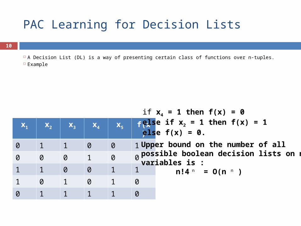
A Decision List (DL) is a way of presenting certain class of functions over n-tuples. Example

10

x1 x2 x3 x4 x5 f(x)

0 1 1 0 0 1

0 0 0 1 0 0

1 1 0 0 1 1

1 0 1 0 1 0

0 1 1 1 1 0

if x4 = 1 then f(x) = 0else if x2 = 1 then f(x) = 1else f(x) = 0.

Upper bound on the number of allpossible boolean decision lists on n variables is :

n!4 n = O(n n )

PAC Learning for Decision Lists

Algorithms : A greedy approach (Rivest, 1987)1. If the example set S is empty, halt.2. Examine each term of length k until a term t is found s.t. all examples in S which make t true are of the same type v.3. Add (t, v) to decision list and remove those examples from S.4. Repeat 1-3. Clearly, it runs in polynomial time.

11

What does PAC do?

12

A supervised learning framework to classify data

How can we use PAC?

Use PAC as a general framework to guide us on efficient sampling for machine learning

Use PAC as a theoretical analyzer to distinguish hard problems from easy problems

Use PAC to evaluate the performance of some algorithms

Use PAC to solve some real problems

13

What we are going to cover?

Explore what PAC can learn

Apply PAC to real data with noise

Give a probabilistic analysis on the performance of PAC

14

PAC Learning for Decision Lists

Algorithms : A greedy approach

15

x1 x2 x3 x4 x5 f(x)

0 1 1 0 0 1

0 0 0 1 0 0

1 1 0 0 1 1

1 0 1 0 1 0

0 1 1 1 1 0

Analysis of Greedy Algorithm

The output

16

Performance Guarantee

PAC Learning for Decision Lists

1. For a given S, by partitioning the set of all concepts that agree with f on S into a “bad” set and a “good”, we want to achieve

2. Consider any h, the probability that we pick S such that h ends up in bad set is

3.

4. Putting together

17

The Limitation of PAC for DLs

18

x1 x2 f(x)

0 0 10 1 01 0 01 1 1

What if the examples are like below?

Other Concept Classes

Decision tree : Dts of restricted size are not PAC-learnable, although those of arbitrary size are.

AND-formulas: PAC-learnable. 3-CNF formulas: PAC-learnable. 3-term DNF formulas: In fact, it turns out that it is an

NP-hard problem, given S, to come up with a 3-term DNF formula that is consistent with S. Therefore this concept class is not PAC-learnable—but only for now, as we shall soon revisit this class with a modified definition of PAC-learning.

19

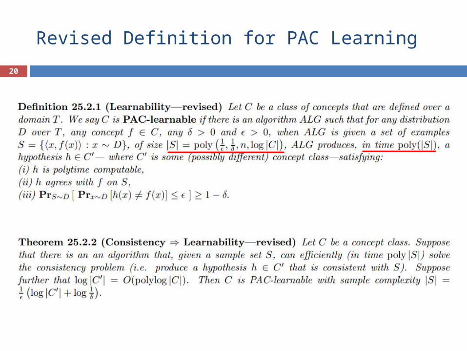
Revised Definition for PAC Learning

20

Weak PAC-Learnability

21

Benefits:To loose the requirements for a highly accurate algorithmTo reduce the running time as |S| can be smallerTo find a “good” concept using the simple algorithm A

Confidence Boosting Algorithm

22

Boosting the Confidence

23

Boosting the Confidence

24

Boosting the Confidence

25

The basic idea exploits the fact that you can learn a little on every distribution and with more iterations we can get much lower error rate.

Error Reduction by Boosting

26

Detailed Steps: 1. Some algorithm A produces a hypothesis that has

an error probability of no more than p = 1/2−γ (γ>0). We would like to decrease this error probability to 1/2−γ with γ > γ.′ ′

2. We invoke A three times, each time with a slightly different distribution and get hypothesis h1, h2 and h3, respectively.

3. Final hypothesis then becomes h=Maj(h1, h2,h3).

Error Reduction by Boosting

27

Learn h1 from D1 with error p Modify D1 so that the total weight of incorrectly marked

examples are 1/2, thus we get D2. Pick sample S2 from this distribution and use A to learn h2.

Modify D2 so that h1 and h2 always disagree, thus we get D3. Pick sample S3 from this distribution and use A to learn h3.

Error Reduction by Boosting

28

The total error probability h is at most 3p^2−2p^3, which is less than p when p (0,1/2). The proof of how to get this probability ∈is shown in [1].

Thus there exists γ > γ such that the error probability of our new ′hypothesis is at most 1/2−γ .′

Error Reduction by Boosting

[1] http://courses.csail.mit.edu/6.858/lecture-12.ps

29

Error Reduction by Boosting

30

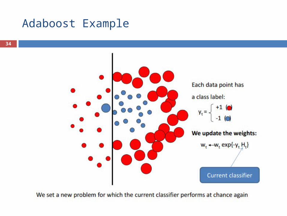
Defines a classifier using an additive model:

Adaboost

31

Adaboost

32

Adaboost Example

33

Adaboost Example

34

Adaboost Example

35

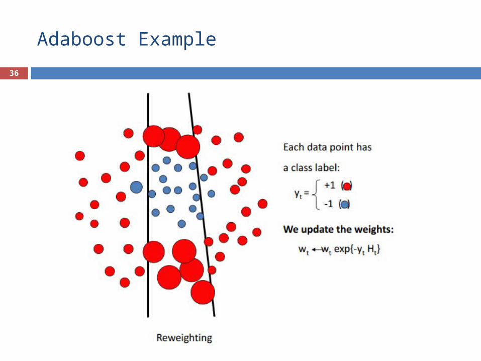
Adaboost Example

36

Adaboost Example

37

Adaboost Example

38

Error Reduction by Boosting

39

Fig. Error curves for boosting C4.5 on the letter dataset as reported by Schapire et al.[]. Training and test error curves are lower and upper curves respectively.

PAC learning conclusion

Strong PAC learning Weak PAC learning Error reduction and boosting

40

Mistake Bound Model of Learning

Mistake Bound Model Predicting from Expert Advice

The Weighted Majority Algorithm Online Learning from Examples

The Winnow Algorithm

41

Mistake Bound Model of Learning | Basic Settings

x – examples c – the target function, ct ∈ C x1, x2… xt an input series at the tth stage

1. The algorithm receives xt

2. The algorithm predicts a classification for xt, bt

3. The algorithm receives the true classification, ct(x).

a mistake occurs if ct(xt) ≠ bt

42

Mistake Bound Model of Learning | Basic Settings

A hypotheses class C has an algorithm A with mistake M: if for any concept c ∈ C, and for any ordering of examples, the total number of mistakes ever made by A is bounded

by M.

43

Mistake Bound Model of Learning | Basic Settings

Predicting from Expert Advice The Weighted Majority Algorithm

Online Learning from Examples The Winnow Algorithm

44

Predicting from Expert Advice

Predicting from Expert Advice The Weighted Majority Algorithm

Deterministic Randomized

45

Predicting from Expert Advice | Basic Flow

Combining Expert AdviceCombining Expert Advice

Prediction

Truth

Assumption: prediction ∈ {0, 1}.

46

Predicting from Expert Advice | Trial

(1) Receiving

prediction from experts

(2) Making its own

prediction

(3) Being told the correct answer

47

Predicting from Expert Advice | An Example

Task : predicting whether it will rain today. Input : advices of n experts ∈ {1 (yes), 0 (no)}. Output : 1 or 0. Goal : make the least number of mistakes.

Expert 1 Expert 2 Expert 3 Truth

21 Jan 2013 1 0 1 1

22 Jan 2013 0 1 0 1

23 Jan 2013 1 0 1 1

24 Jan 2013 0 1 1 1

25 Jan 2013 1 0 1 1

48

The Weighted Majority Algorithm | Deterministic

49

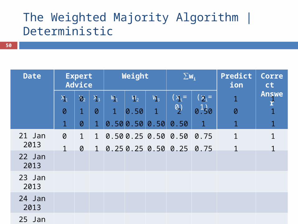
The Weighted Majority Algorithm | Deterministic

Date Expert Advice Weight ∑wi Prediction Correct Answerx1 x2 x3 w1 w2 w3 (xi=0) (xi=1)

21 Jan 2013

22 Jan 2013

23 Jan 2013

24 Jan 2013

25 Jan 2013

1

0

1

0

1

0

1

0

1

0

1

0

1

1

1

1

1

0.50

0.50

0.25

1

0.50

0.50

0.25

0.25

1

1

0.50

0.50

0.50

1

2

0.50

0.50

0.25

2

0.50

1

0.75

0.75

1

0

1

1

1

1

1

1

1

1

50

The Weighted Majority Algorithm | Deterministic

Proof: Let

M := # of mistakes made by Weight Majority algorithm. W := total weight of all experts (initially = n).

A mistaken prediction: At least ½ W predicted incorrectly.

In step 3 total weight reduced by a factor of ¼ (= ½ W x ½). W ≤ n(¾)M

Assuming the best expert made m mistakes. W ≥ ½m

So, ½m ≤ n(¾)M M ≤ 2.41(m + lgn).

51

The Weighted Majority Algorithm | Randomized

View as Probability

Multiply by β

52

The Weighted Majority Algorithm | Randomized

Advantages Dilutes the worst case:

Worst Case: slightly > ½ of the weights predicted incorrectly. Simple Version: make a mistake and reduce total weight by ¼. Randomized Version: has a 50/50 chance to predicate correctly.

Selecting an expert with probability proportional to its weight: Feasibility: (e.g., when weights cannot be easily combined). Efficiency: (e.g., when the experts are programs to be run or

evaluated).

53

The Weighted Majority Algorithm | Randomized

54

The Weighted Majority Algorithm | Randomized

β = ½ then M < 1.39m + 2ln n β = ¾ then M < 1.15m + 4ln n Adjusting β to make the “competitive ratio” as close to 1 as desired.

55

Mistake Bound Model of Learning

Mistake Bound Model Predicting from Expert Advice

The Weighted Majority Algorithm Online Learning from Examples

The Winnow Algorithm

56

Online Learning from Examples

Weighted Majority Algorithm is “learning from expert advice” Recall Offline learning V.S. Online Learning

Offline learning: training dataset => learning the model parameters Online learning: each “training” instance comes like a stream =>

update the model parameters after receiving each instance Recall the Mistake Bound Model (Online learning):

At each iteration:

Goal: Minimize the number of mistakes made.

Receive a feature vector

x

Receive x’s true label: c

Predict x’s label: b

Update the model params

57

Winnow Algorithm

Simple Winnow Algorithm: Each input vector x = {x1, x2, … xn}, xi {0, 1}∈ Assume the target function is the disjunction of r

relevant variables. I.e. f(x) = xt1 V xt2 V … V xtr

Winnow algorithm provides a linear separator

58

Winnow Algorithm

Initialize: weights w1 = w2 = … = wn=1 Iterate:

Receive an example vector x = {x1, x2, … xn} Predict:

Output 1 if Output 0 otherwise

Get the true label Update if making a mistake:

False positive error: for each xi = 1: wi = 2*wi False negative error: for each xi = 1: wi = wi/2

59

Difference with Weighted Majority Algorithm?

Analysis of Simple Winnow

Assumption: the target function is the disjunction of r relevant variables and remains unchanged

Bound: #total mistakes ≤ 2 + 3r(1+log n) Analysis & Proof

False Positive errors: The true label is +1 because at least ONE relevant variable(xt) is 1 Error is caused by x w∙ < n => wt < n Update rule: wt = wt * 2 => #error when xt=1 is at most (1+log n) The false positive error bound is r(1+log n)

False Negative error: The similar analysis procedure can get the bound 2+2r(1+log n)

60

Extensions of Winnow…

Examples are not exactly match the target function: Error bound is O(r m∙ c + r lg n)∙

mc is the errors made by the target function It means Winnow has a O(r)-competitive error bound.

The target function may change with time: Imagine an adversary(enemy) changes the target function by

adding or removing variables. The error bound is O(cA ∙ log n)

61

Extensions of Winnow…

The feature variable is continuous rather than boolean Theorem: if the target function is embedding-closed, then

Winnow can also be learned in the Infinite-Attribute model

By adding some randomness in the algorithm, the bound can be further improved.

62

PAC versus MBM (Mistake Bound Model)

Intuitively, MBM is stronger than PAC MBM gives the determinant error upper bound PAC guarantees the mistake with constant probability

A natural question: if we know A learns some concept class C in the MBM, can A learn the same C in the PAC model? Answer: Of course! We can construct APAC in a

principled way [1]

63

Conclusion

PAC (Probably Approximately Correct) Easier than MBM model since examples are restricted to

be coming from a distribution. Strong PAC and weak PAC Error reduction and boosting

MBM(Mistake Bound Model) Stronger bound than PAC: exactly upper bound of errors 2 representative algorithms

Weighted Majority: for online expert learning Winnow: for online linear classifier learning

Relationship between PAC and MBM

64

Q & A

65

References

[1] Tel Aviv University’s Machine Lecture: http://www.cs.tau.ac.il/~mansour/ml-course-10/scribe4.pdf Machine Learning Theory http://www.cs.ucla.edu/~jenn/courses/F11.html http://www.staff.science.uu.nl/~leeuw112/soiaML.pdf PAC www.cs.cmu.edu/~avrim/Talks/FOCS03/tutorial.ppt http://www.autonlab.org/tutorials/pac05.pdf http://www.cis.temple.edu/~giorgio/cis587/readings/pac.html Occam’s Razor http://www.cs.iastate.edu/~honavar/occam.pdf The Weighted Majority Algorithm http://www.mit.edu/~9.520/spring08/Classes/online_learning_2008.pdf http://users.soe.ucsc.edu/~manfred/pubs/C50.pdf http://users.soe.ucsc.edu/~manfred/pubs/J24.pdf The Winnow Algorithm http://www.cc.gatech.edu/~ninamf/ML11/lect0906.pdf http://stat.wharton.upenn.edu/~skakade/courses/stat928/lectures/lecture19.pdf http://www.cc.gatech.edu/~ninamf/ML10/lect0121.pdf

66

Supplementary Slides67

Chernoff’s Bound

Chernoff bounds are another kind of tail bound. Like Markoff and Chebyshev, they bound the total amount of probability of some random variable Y that is in the “tail”, i.e. far from the mean.

For detailed derivation for Chernoff bounds, you may refer to http://www.cs.cmu.edu/afs/cs/academic/class/15859-f04/www/scribes/lec9.pdf

http://www.cs.berkeley.edu/~jfc/cs174/lecs/lec10/lec10.pdf

68

Proof of Theorem 2 (1/2)

69

Proof of Theorem 2 (2/2)

70

Corollary 3:

71