SYNTHESIS OF BIOPROCESSES USING PHYSICAL PROPERTIES DATA

M.A. Steffens, E.S. Fraga and I.D.L. Bogle 1

Department of Chemical Engineering, University College London.

Short title: Bioprocess Synthesis.

November 24, 2000

1Corresponding author: I.D.L. Bogle, Department of Chemical Engineering, University CollegeLondon, Torrington Place, London, WC1E 7JE. Phone: +44 (0)171 419 3803. Fax: +44 (0)171 383 2348.Email: d.bogle@ucl.ac.uk.

Abstract

The aim of this paper is to illustrate and evaluate a synthesis technique for bioprocesses.Physical property information is used to screen candidate units thereby reducing the sizeof the synthesis problem. In this way only units which exploit large property differencesbetween components in a stream are selected. This is important for bioprocesses becauseof the large number of components and wide range of unit operations which are available.The screening technique and bioprocess unit design methodologies have been incorporatedwithin an implicit enumeration algorithm which was developed for chemical process syn-thesis and is implemented in the Java language. An important advantage is its ability togenerate a ranked list of N flowsheets which may subsequently be analysed in more detail.

Two case studies are used to evaluate the bioprocess synthesis technique. The first systeminvolves a product which is secreted from the host organism while the second has signifi-cantly different characteristics in that the product is intracellular and forms inclusion bodies.The second case study, in particular, is a large synthesis problem with 12 unit operations and20 contaminant compounds considered. The results show that the synthesis methodologyidentifies a set of economically optimal flowsheets in a reasonable computational time whichdemonstrates its ability to deal with large synthesis problems. Using the synthesis method-ology we can generate bioprocesses which are optimal in a system wide, rather than unit byunit, sense.

Keywords: process synthesis, bioprocesses, physical properties, optimisation.

1 Introduction

New product development is an integral part of the biochemical production industry dueto the large range of biological products which are potentially valuable to society. Once anew product has been developed in the laboratory, however, a process which can produceand purify the product in large quantities is required. The success of a biochemical com-pounds manufacturing company may depend on the ability to design such a process in aneconomically optimal way (Leser and Asenjo, 1992; Wheelwright, 1987). For bioprocessesin particular, it is important to choose the optimal system as early as possible in the designprocedure. This is because a process’ characteristics are fixed once approved by the relevantregulatory body. Subsequent changes must go through a further expensive approval process(Petrides et al., 1995).

Bioprocess flowsheets are often synthesised in a sequential fashion, proceeding from oneunit to the next until product specifications are met (Wheelwright, 1987). Individual unitsare subsequently optimised to improve plant performance. Although this approach mayproduce economically adequate processes, alternative designs may be more profitable. Toavoid this problem we require a systematic synthesis and design procedure which considersthe overall process, rather than individual units (Wheelwright, 1987).

There currently exists a large body of literature on systematic process synthesis and designmethods for chemical processes. These can be broadly classified into heuristic based ap-proaches, such as the work by Douglas (1988), and algorithmic techniques (e.g. Fraga andMcKinnon, 1994; Friedler et al., 1996; Grossman and Kravanja 1995; Smith and Pantelides,1995). The same abundance of literature does not exist for bioprocess synthesis techniques.Notable exceptions include work presented by Petrides (1994), who developed a synthesisprocedure which uses expert knowledge to select unit operations. Lienqueo et al. (1996) de-scribe a synthesis methodology which uses a combination of expert knowledge and physicalproperties data to synthesise downstream purification flowsheets. Both of these approachesare capable of synthesising economically favorable processes and represent significant ad-vances in the field of bioprocess synthesis. However, two important characteristics of thesynthesis techniques should be noted:

1. the use of expert knowledge may lead to the elimination of novel flowsheets whichseem to contravene prevailing experience yet have interesting or desirable features.

2. both synthesis techniques treat the recovery and high resolution purification sectionsof a bioprocess as separate entities. This means that although each section of the plantmay be optimally designed, the same cannot be said of the whole process.

Algorithms which are based on mathematical optimisation techniques provide a more rigor-ous approach to synthesis which allows us to avoid the above two shortcomings. However,when attempting to apply optimisation methods to solve the bioprocess synthesis problemwe encounter several major obstacles:

� Unit operations commonly used for downstream purification generally separate com-ponents non-sharply. A non-sharp separation is one in which the feed components aredistributed between the effluent streams.

1

� A large selection of unit operations is available.

� Biological streams generally contain a large number of compounds.

These characteristics lead to a large number of alternative feasible flowsheets and, therefore,a correspondingly large search space for the synthesis algorithm (Fraga, 1996b; Lienqueo etal., 1996). Synthesis problems of this size are difficult to solve using numerical optimisationtechniques.

Fraga (1998) described the Jacaranda synthesis package which is capable of tackling problemswith the characteristics described above. It is based on the use of discretisation to convertthe mixed integer nonlinear programming (MINLP) problem into a graph generation andsearch problem. Continuous variables, such as stream compositions and properties and unitdesign parameters, are mapped to a discrete space using discretisation parameters chosenby the user. In this paper we extend the Jacaranda process synthesis package to incorporatebioprocess synthesis.

On application of the technique, however, the authors found that the use of discretisationalone was not sufficient to make bioprocess synthesis problems tractable. Therefore, thenumber of synthesis alternatives is further reduced by screening candidate units using phys-ical properties data. In this way we select units which best exploit the physical propertiesdifferences between the components in a bioprocess stream. The technique is evaluated byapplying it to the synthesis of flowsheets for the purification of two industrially producedbiochemical products.

2 The Bioprocess Synthesis Methodology

The Jacaranda system (Fraga, 1998) is a software implementation of an implicit enumerationprocedure for automated synthesis. Based on a discrete programming approach, Jacarandais suitable for solving the downstream purification flowsheet synthesis problem because ithas the following features:

� Many numerical synthesis algorithms require the user to specify a superstructure con-taining all possible flowsheet alternatives beforehand (e.g. Grossman and Kravanja,1995; Smith and Pantelides, 1995). Defining a superstructure is difficult for biochem-ical systems which have many components, a large number of possible units and usenon-sharp separators. In addition, the optimal flowsheet is not guaranteed to be in-cluded within the superstructure. Jacaranda, however, simultaneously generates andsearches the superstructure using a discrete implicit enumeration method.

� The screening methodology is easily incorporated into the search procedure and sig-nificantly reduces ( � 50%) the size of the superstructure as we will show later.

� Complex models may be included because a discrete optimisation is used thereby mak-ing the algorithm computationally efficient. This is particularly useful for bioprocesseswhich are often operated in a batch fashion (Petrides, 1994). Unit models for batchprocesses often consist of sets of time dependent differential equations which must

2

be integrated (e.g. Steffens et al., 1999). In addition the search procedure imposes norequirements on the models convexity and continuity.

Jacaranda has been implemented in the JAVA language and uses two basic data structures,or classes, which are required to synthesise a process flowsheet: the Stream and UnitModelclasses. As the name suggests the Stream class is a data structure which represents a processstream. For instance, in the synthesis of bioprocesses a stream class may contain informa-tion on the concentrations of each component (e.g. cells, secreted proteins etc), the physicalproperties for each component and the stream flow rate.

Also required is a UnitModel class for each type of unit operation which the user wishes toconsider during the synthesis procedure. UnitModel classes contain the physical propertiesscreening steps along with design equations which are used to determine the composition,flow and number of streams leaving each unit. In addition, capital and operating costs areestimated within UnitModel classes. A detailed discussion of the bioprocess unit design andcost estimation techniques used in this work is presented later.

To convert the synthesis problem from a mixed integer non-linear program (MINLP) into adiscrete optimisation problem the Jacaranda package converts all continuous variables intodiscrete values. In bioprocess synthesis, there are two types of continuous variables whichmust be discretised:

� stream characteristics such as components flow rates. The discretisation level (or baseflow) for these variables may be chosen by the user. For example, the base flow rate forwater may be set to 5

�������. This means that the mass flow of water will be rounded

to the nearest multiple of 5 for each stream created during a synthesis run.

� unit design parameters such as the operating pH in an ion-exchange column. Designparameters may be considered as degrees of freedom during synthesis and design. Arange and discretisation level for design parameters can also be specified by the user.For example, the pH in an ion-exchange column may be allowed to vary from 4 to 8in steps of 2. The synthesis method designs the unit at each of the discrete values andevaluates each design.

The Jacaranda algorithm uses implicit enumeration to simultaneously generate and searchall possible flowsheets in the discrete space in a depth first manner. To begin with, the feedstream is passed to each unit model and if a unit can process the stream then the compositionand state of any stream(s) leaving the unit are calculated. From there the same procedure isrepeated for each new stream. The algorithm continues until units which do not produce anystreams are encountered. Such terminating units, or product tanks, are defined so as onlyto accept streams which contain a product at the desired purity. Computational efficiency isachieved in two ways:

1. Dynamic programming: Due to the discrete nature of the synthesis methodology it ispossible for streams with the same composition and properties to arise via differentsynthesis routes. When stream characteristics are identical, the flowsheeting possibil-ities for processing the stream are also identical. In the Jacaranda process synthesis

3

package computational effort is reduced by identifying situations in which identicalstreams arise, and synthesising the corresponding flowsheets only once. Of course wecan only check whether streams have the same composition in a discrete sense. To dothis the Stream class must have a unique ‘key’ string for identification purposes (Fraga,1996b).

2. Cost pruning: branches in the search graph may be pruned if their cost exceeds that ofa different alternative before the branch has been exhaustively searched.

We now discuss the bioprocess unit design and costing methods in detail.

2.1 Unit Design Techniques

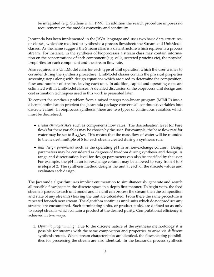
The bioprocess unit design procedure consists of a preliminary screening procedure fol-lowed by the actual design calculations which are used to determine effluent stream charac-teristics and cost information. The design procedure is summarised in Figure 1.

1. Check constraints

Pass

Pass

Design Ok

3. Binary ratio check

4. Design unit, determine effluent

stream characteristics and estimate costs

Fail

Begin

Design Failed

2. Choose design parameters

5. Move to next set of parameters

Fail

Figure 1: The bioprocess unit screening and design procedure

In general, bioprocesses can be considered to consist of two subprocesses: fermentation anddownstream purification (Lienqueo et al., 1996). In this paper we focus upon the downstreampurification section of the process. The effects of fermenter design issues on bioprocess syn-thesis have been investigated elsewhere (Steffens et al., 1999).

2.1.1 Screening Units During Synthesis

The bioprocess synthesis algorithm developed in this work uses physical properties infor-mation to screen units thereby reducing the search space. This is advantageous becausebioprocesses usually involve non-sharp separations and have many different available tech-nologies which makes the search space large. Two types of tests are used to eliminate unitswhich are not feasible for a particular separation:

4

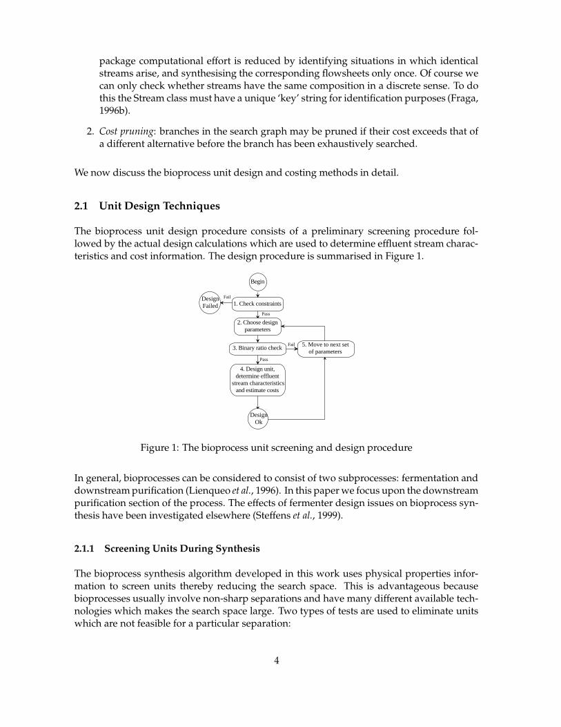
1. Design constraints which are physical limits on pieces of equipment. For example,packed bed chromatography columns cannot process streams which contain solids.Table 1 summarises the design constraints used in this work.

2. The binary ratio check which utilises the concept of a key property, or driving force,which each unit exploits to achieve separation. This is discussed in more detail below.

Table 1: Bioprocess unit design constraintsUnit Constraints � Source

Ultrafilter �� ����������� ������ � Asenjo (1990) pp 210������� ���! �"!#�%$&��' ���! �"!#Microfilter �(�! �)�*���*�+�,�� � Asenjo (1990) pp 210� $.- ��' ���! �"!# Ho and Sirkar (1992) pp577Diafilter �/��������� ������ � Asenjo (1990) pp 210������0 ���! �"!#Centrifuge � � ��� �1- � � ' �! �"!# Kennedy and Cabral (1993) pp 169Rotary drum filter � �2�! �3�*�4�5�� � Gabler (1985)���1-6�87 �:95;&"1; Kennedy and Cabral (1993) pp 87Chromatography �����<7 �! �"!# Leser and Asenjo (1992)column No solids in the feedHomogeniser � �1- �=7�' �! �"!# Wheelwright (1991) pp64

The use of physical properties information for bioprocess synthesis is not a new concept.In the downstream processing design methodology described by Wheelwright (1987), it isrecommended that the engineer selects units which exploit the greatest differences in phys-ical properties between components. Leser and Asenjo (1992) go a step further and definea separation coefficient which is a function of the physical properties difference betweencomponents and may be used to choose between high resolution purification operations.

In this work we use a method developed by Jaksland et al. (1995) for chemical process syn-thesis to screen out infeasible unit operations for bioprocesses. Each separation process,whether chemical or biochemical, exploits specific property differences to facilitate purifica-tion of the various components in a stream. In this synthesis approach the key driving force,and corresponding property, utilised by each technology is identified (Table 2). To determinethe applicability of any particular unit operation for the separation of a pair of componentsthe ratio of this property (binary ratio) is calculated for each pair. If it is large enough thenthe unit is considered feasible for the separation.

A simple test is used to identify candidate separation operations by comparing two numbers:

1. Binary ratios: the potential driving force for the separation of any two components isquantified by calculating the ratio of the physical property governing the separation inthe unit being considered (binary ratio).>

See ? 6 for symbol definitions

5

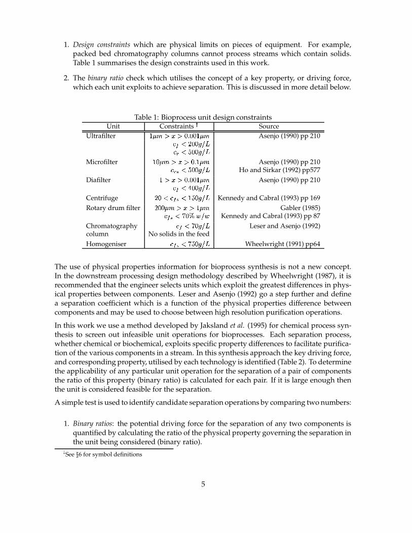
Table 2: Physical properties used by bioprocess unit operationsUnit Operation Physical property @ Source

Centrifugation Settling velocity 1.1Conventional filtration Size (particle) 1.1Rotary drum filtration Size (particle) 1.1Microfiltration Size (particle) 3.0 Jaksland et al. (1995)Ultrafiltration Size (molecular) 3.0 Jaksland et al. (1995)Diafiltration Size (molecular) 3.0 Jaksland et al. (1995)Ion exchange Net charge 2.5Gel chromatography log(Mol. Wt.) 1.05Hydrophobic Int. Chr. Hydrophobicity 1.5

2. Feasibility indices: the binary ratios are then compared to feasibility indices, A , whichare predefined constants for each separation technology. The indices define how largethe binary ratio must be before a separation is feasible. Suggested values for A areshown in Table 2. Where sources are omitted recommended values were based on ananalysis of the sensitivity of the synthesis results to the feasibility indices. Details of theinvestigation, which was performed using the first case study system, are presentedbelow.

In combination, the design constraints and physical properties screening techniques reducethe problem size thereby making the synthesis problem simpler to solve without eliminat-ing economically desirable processes. When a candidate unit passes the screening tests fora particular separation we proceed with the design and costing calculations for that unit.These are now described in detail.

2.1.2 Design and Cost Estimation Techniques

Two different approaches are used to determine the effluent stream characteristics for a sep-aration unit depending upon the unit type: splitting or fractionating units. The former oper-ate in a more traditional chemical engineering sense, that is by splitting the incoming streaminto two with significantly different composition, hence achieving separation. The latter,however, generally operate batchwise and produce several fractions or cuts. Chromatog-raphy columns, where the various components are eluted sequentially, are a particularlycommon example of a fractionating unit.

Stream Splitting Units

Units which operate in a stream splitting sense are designed using a similar concept to thatused in shortcut distillation design. The design procedure is based on the assumption thateach unit operation exploits a particular physical property to achieve separation (Table 2).Initially, a list of the feed components, ordered in terms of this physical property, is generat-ed. Two ‘key’ components are selected as an adjacent pair from this list. Prior to any designcalculations, the binary ratio of the two key components is calculated and compared withthe feasibility index for the unit under consideration. If the binary ratio is greater than thefeasibility index, the design calculations are performed.

6

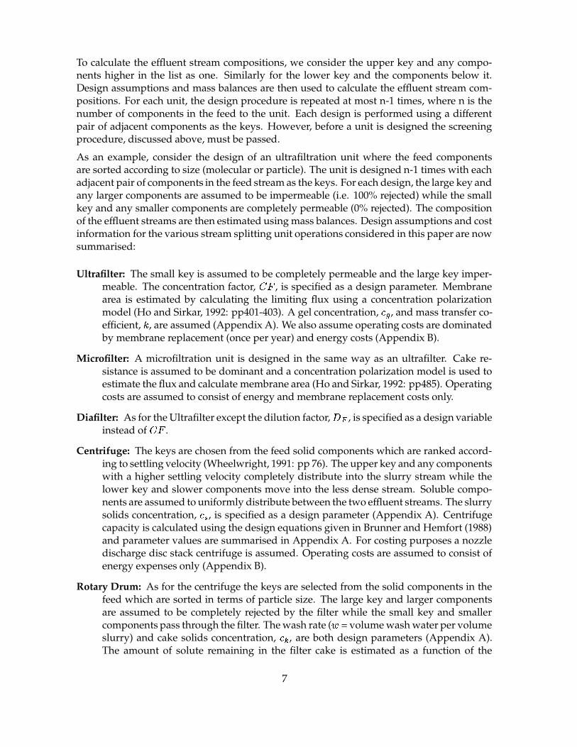
To calculate the effluent stream compositions, we consider the upper key and any compo-nents higher in the list as one. Similarly for the lower key and the components below it.Design assumptions and mass balances are then used to calculate the effluent stream com-positions. For each unit, the design procedure is repeated at most n-1 times, where n is thenumber of components in the feed to the unit. Each design is performed using a differentpair of adjacent components as the keys. However, before a unit is designed the screeningprocedure, discussed above, must be passed.

As an example, consider the design of an ultrafiltration unit where the feed componentsare sorted according to size (molecular or particle). The unit is designed n-1 times with eachadjacent pair of components in the feed stream as the keys. For each design, the large key andany larger components are assumed to be impermeable (i.e. 100% rejected) while the smallkey and any smaller components are completely permeable (0% rejected). The compositionof the effluent streams are then estimated using mass balances. Design assumptions and costinformation for the various stream splitting unit operations considered in this paper are nowsummarised:

Ultrafilter: The small key is assumed to be completely permeable and the large key imper-meable. The concentration factor, BDC , is specified as a design parameter. Membranearea is estimated by calculating the limiting flux using a concentration polarizationmodel (Ho and Sirkar, 1992: pp401-403). A gel concentration, E:F , and mass transfer co-efficient,

�, are assumed (Appendix A). We also assume operating costs are dominated

by membrane replacement (once per year) and energy costs (Appendix B).

Microfilter: A microfiltration unit is designed in the same way as an ultrafilter. Cake re-sistance is assumed to be dominant and a concentration polarization model is used toestimate the flux and calculate membrane area (Ho and Sirkar, 1992: pp485). Operatingcosts are assumed to consist of energy and membrane replacement costs only.

Diafilter: As for the Ultrafilter except the dilution factor, GIH , is specified as a design variableinstead of BDC .

Centrifuge: The keys are chosen from the feed solid components which are ranked accord-ing to settling velocity (Wheelwright, 1991: pp 76). The upper key and any componentswith a higher settling velocity completely distribute into the slurry stream while thelower key and slower components move into the less dense stream. Soluble compo-nents are assumed to uniformly distribute between the two effluent streams. The slurrysolids concentration, E�J , is specified as a design parameter (Appendix A). Centrifugecapacity is calculated using the design equations given in Brunner and Hemfort (1988)and parameter values are summarised in Appendix A. For costing purposes a nozzledischarge disc stack centrifuge is assumed. Operating costs are assumed to consist ofenergy expenses only (Appendix B).

Rotary Drum: As for the centrifuge the keys are selected from the solid components in thefeed which are sorted in terms of particle size. The large key and larger componentsare assumed to be completely rejected by the filter while the small key and smallercomponents pass through the filter. The wash rate ( K = volume wash water per volumeslurry) and cake solids concentration, E�L , are both design parameters (Appendix A).The amount of solute remaining in the filter cake is estimated as a function of the

7

wash rate (Kennedy and Cabral, 1993: pp 90). To estimate the filter area we assume aconstant specific cake resistance (Belter et al., 1988). For parameter values see AppendixA. Operating costs include energy and filter aid expenses only (Appendix B).

Fractionating Units

Chromatography columns, which fractionate rather than split, cannot be designed using thekey component technique. The elution profile must be estimated so that the amount of eachcontaminant which leaves with the desired product can be estimated.

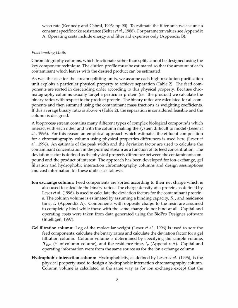
As was the case for the stream splitting units, we assume each high resolution purificationunit exploits a particular physical property to achieve separation (Table 2). The feed com-ponents are sorted in descending order according to this physical property. Because chro-matography columns usually target a particular protein (i.e. the product) we calculate thebinary ratios with respect to the product protein. The binary ratios are calculated for all com-ponents and then summed using the contaminant mass fractions as weighting coefficients.If this average binary ratio is above A (Table 2), the separation is considered feasible and thecolumn is designed.

A bioprocess stream contains many different types of complex biological compounds whichinteract with each other and with the column making the system difficult to model (Leser etal., 1996). For this reason an empirical approach which estimates the effluent compositionfor a chromatography column using physical properties differences is used here (Leser etal., 1996). An estimate of the peak width and the deviation factor are used to calculate thecontaminant concentration in the purified stream as a function of its feed concentration. Thedeviation factor is defined as the physical property difference between the contaminant com-pound and the product of interest. The approach has been developed for ion-exchange, gelfiltration and hydrophobic interaction chromatography columns and design assumptionsand cost information for these units is as follows:

Ion exchange column: Feed components are sorted according to their net charge which isalso used to calculate the binary ratios. The charge density of a protein, as defined byLeser et al. (1996), is used to calculate the deviation factors for the contaminant protein-s. The column volume is estimated by assuming a binding capacity, MON , and residencetime, PRQ (Appendix A). Components with opposite charge to the resin are assumedto completely bind while those with the same charge do not bind at all. Capital andoperating costs were taken from data generated using the BioPro Designer software(Intelligen, 1997).

Gel filtration column: Log of the molecular weight (Leser et al., 1996) is used to sort thefeed components, calculate the binary ratios and calculate the deviation factor for a gelfiltration column. Column volume is determined by specifying the sample volume,M JTS%U (% of column volume), and the residence time, P Q (Appendix A). Capital andoperating information were from the same source as for the ion exchange column.

Hydrophobic interaction column: Hydrophobicity, as defined by Leser et al. (1996), is thephysical property used to design a hydrophobic interaction chromatography column.Column volume is calculated in the same way as for ion exchange except that the

8

binding fraction, CWV , for each component is assumed to have a linear relationship withthe hydrophobicity, X . Cost information is also from Intelligen (1997).

In addition to the separation units described thus far there are two important processeswhich do not separate components and, therefore, do not fit into either category: homogeni-sation and renaturation. Their design and cost assumptions are now discussed:

Homogeniser: We assume a high pressure homogeniser and specify the percentage recov-ery (Appendix A). The average size of the cell debris is also specified. Operating costsconsist of energy expenditure only (Appendix B).

Renaturing tank: When the product protein forms inclusion bodies a solubilisation and re-naturing tank is required. This unit is designed by specifying a residence time, P Q , andyield, Y (Appendix A). The incoming stream is diluted with water to achieve a spec-ified protein concentration (Appendix A). Capital costs are estimated as for a stirredtank and chemical costs are assumed to be the major operating expense (Appendix B).

In addition to capital and operating costs, we must estimate the value of the product andbalance this against expenses. A logical way to do this is to use a negative cost (i.e. revenue)for any product which meets the required specifications. However, a cost scheme whichincorporates solely positive cost data is advantageous to make best use of cost pruning inthe synthesis algorithm. To achieve this we have used the following scheme: zero cost forany product leaving the process which meets specifications; and a positive cost for productwhich does not (i.e. wasted product). This cost scheme drives the synthesis process towardsthe production of on-specification product without using negative costs.

2.2 Enhancements to Jacaranda

The Jacaranda system provides an extensible framework for process synthesis. Through thedefinition of appropriate Stream and UnitModel classes, the search procedure is extended toinclude screening based on physical properties. However, there are two aspects of Jacarandawhich have been enhanced to cater for the special properties of biochemical process synthe-sis:

1. The large size of the search space makes it worthwhile to introduce an extra pruningoperation.

2. The ability to generate a ranked list of N solutions, instead of just the optimal flow-sheet, has been enhanced to increase the diversity of solutions presented for any givenvalue of N.

These two extensions are now described in more detail.

9

2.2.1 Heuristic Leaf Pruning

At each node in the search graph, the system considers each of the available units in turn. Ifa unit can handle the stream associated with the node, the set of discrete alternative designsare then processed. The outputs of each alternative become new nodes in the recursivesearch procedure. Because the search only backtracks when a node can only be processed byunits which are final product or waste tanks, the depth of the search graph can be arbitrarilylarge when non-sharp separations are allowed. The ability to selectively but automaticallyprune some of the branches in the search procedure is necessary in these cases to ensure thatsolutions can be found in reasonable time.

The system has been extended to allow the depth-first search to terminate when a stream isfound to match the criteria associated with a product or waste tank. Instead of consideringall units that can handle a given stream, the order of the units in the problem definitionbecomes a heuristic which can eliminate unnecessary searching. For example, if units areordered so that the main product tank comes first, any stream which is a valid product willnot be processed further.

Although the addition of this heuristic to the search procedure reduces the search space, itdoes so fully under user control. Only those product or waste tank units which have strictcriteria will typically be placed at the beginning of the list of units. In Section 3.1, we use acase study to quantify the reduction in the size of the search space which can be achievedusing the leaf prune feature.

2.2.2 Enhancing N-best diversity

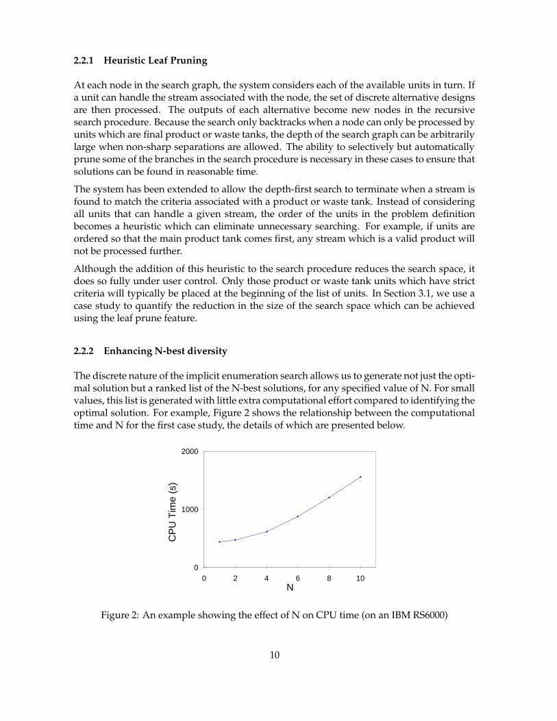
The discrete nature of the implicit enumeration search allows us to generate not just the opti-mal solution but a ranked list of the N-best solutions, for any specified value of N. For smallvalues, this list is generated with little extra computational effort compared to identifying theoptimal solution. For example, Figure 2 shows the relationship between the computationaltime and N for the first case study, the details of which are presented below.

0

1000

2000

0 2 4 6 8 10N

CP

U T

ime

(s)

Figure 2: An example showing the effect of N on CPU time (on an IBM RS6000)

10

The list of solutions generated by the synthesis algorithm should differ in aspects which areof interest to the designer. For example, generating several solutions which have identicalstructure but differ in some operating condition may not provide enough diversity for thedesign engineer.

For biochemical processes, this diversity may not be enough due to the variety of processingsteps, the degree of non-sharpness and uncertainty in cost models. For example, considera stream with three components, ABC, of which A is the desired product and B and C arewaste products. Figure 3 shows two possible solutions to the synthesis problem (note: aBCdenotes a stream containing a small amount of A and significant amounts of B and C).

ABC aBC

A

Separation process

Product tank

Waste tank

ABC aBC

A

Separation process

Product tank

Separation process

Waste tank

Waste tank

aB

C

Figure 3: An example showing lack of solution diversity

For the engineer, there is really only one interesting feature which is common to both solu-tions: the product A is separated from the initial stream first. However, it is possible thatboth of the structures presented in Figure 3 are cheaper than any more interesting alterna-tives which would not be presented if the engineer had only asked for the two best solutions.

To increase the diversity of flowsheets generated by the synthesis algorithm we have extend-ed the procedure for encoding of solution structures, which is used to compare solutions, toinclude the concept of interesting product nodes. Any structure which does not lead to aninteresting product, as defined by the user, is encoded simply as ”...”. In the example above,if only a product tank is marked as interesting the two solutions in Figure 3 have the sameencoding which means a different alternative would be ranked second thereby increasingthe diversity.

3 Results

Two case studies have been chosen to illustrate the use of the synthesis algorithm and thenew BioStream and UnitModel classes. Firstly we wish to synthesise a downstream flow-sheet for a process where a protein which is secreted from S. Cerevisae is to be purified. Incontrast, the second case study involves the purification of bovine somatotropin (BST), a

11

product which forms inclusion bodies within the E. coli host cells. We now discuss the casestudy details and synthesis results in detail.

3.1 A Secreted Protein

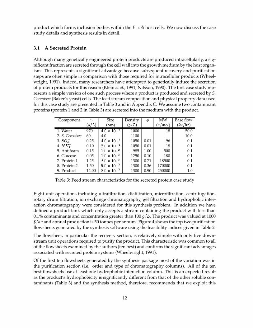
Although many genetically engineered protein products are produced intracellularly, a sig-nificant fraction are secreted through the cell wall into the growth medium by the host organ-ism. This represents a significant advantage because subsequent recovery and purificationsteps are often simple in comparison with those required for intracellular products (Wheel-wright, 1991). Indeed, many researchers have attempted to genetically induce the secretionof protein products for this reason (Klein et al., 1991; Nilsson, 1990). The first case study rep-resents a simple version of one such process where a product is produced and secreted by S.Cerevisae (Baker’s yeast) cells. The feed stream composition and physical property data usedfor this case study are presented in Table 3 and in Appendix C. We assume two contaminantproteins (protein 1 and 2 in Table 3) are secreted into the medium with the product.

Component ��Z Size Density [ MW Base flow( �"!# ) ( � ) ( +"\# ) ( +"1�O]\^ ) ( _: +"!`+a )

1. Water 970 0 � ��bc���+d�e 1000 18 50.02. S. Cerevisae 60 4.0 1100 10.03. fhg de 0.25 0 � ��bi�(��d�e 1050 0.01 96 0.14. j�kmle 0.10 � � ��bi�(��d�e 1050 0.01 18 0.15. Antifoam 0.15 �2� ��bc���+don 985 1.00 500 0.16. Glucose 0.05 �2� ��bc���+dop 1250 0.10 180 0.17. Protein 1 1.25 � � ��bc���+dop 1300 0.71 18500 0.18. Protein 2 1.50 ' � ��bc���+dop 1300 0.36 170000 0.19. Product 12.00 q+� ��bc���+dop 1300 0.90 250000 1.0

Table 3: Feed stream characteristics for the secreted protein case study

Eight unit operations including ultrafiltration, diafiltration, microfiltration, centrifugation,rotary drum filtration, ion exchange chromatography, gel filtration and hydrophobic inter-action chromatography were considered for this synthesis problem. In addition we havedefined a product tank which only accepts a stream containing the product with less than0.1% contaminants and concentration greater than 100

���:r. The product was valued at 1000s �����

and annual production is 50 tonnes per annum. Figure 4 shows the top two purificationflowsheets generated by the synthesis software using the feasibility indices given in Table 2.

The flowsheet, in particular the recovery section, is relatively simple with only five down-stream unit operations required to purify the product. This characteristic was common to allof the flowsheets examined by the authors (ten best) and confirms the significant advantagesassociated with secreted protein systems (Wheelwright, 1991).

Of the first ten flowsheets generated by the synthesis package most of the variation was inthe purification section (i.e. order and type of chromatography columns). All of the tenbest flowsheets use at least one hydrophobic interaction column. This is an expected resultas the product’s hydrophobicity is significantly different from that of the other soluble con-taminants (Table 3) and the synthesis method, therefore, recommends that we exploit this

12

Fermentor

Hydrophobic interaction

chromatography

Ultrafilter

Product tank

Water Buffer +

waste proteins

Buffer + waste

proteins

Water + buffer

Ultrafilter

Hydrophobic interaction

chromatography Rotary drum filter

Cells + filter aid

Fermentor

Hydrophobic interaction

chromatography

Ultrafilter

Product tank

Water Buffer +

waste proteins

Buffer + waste

proteins

Water + buffer

Ultrafilter

Ion exchange

chromatography Rotary drum filter

Cells + filter aid

# 1

# 2

Figure 4: Best two flowsheets identified by the synthesis software

difference. Ion exchange columns also featured in many of the flowsheets generated by thesynthesis software.

The alternatives considered by the synthesis software for cell removal included rotary drumfiltration, centrifugation and cross flow filtration. In the biotechnology industry this deci-sion is a contentious one at present as all three technologies have associated advantages anddisadvantages. In particular, the analysis presented by Tutunjian (1986) showed that crossflow filters have lower capital and operating costs when separating streams containing s-maller bacterial cells (e.g. E. coli). However, for larger cells, as is the case here, centrifugesand rotary drum filters are capable of a higher throughput and, therefore, become more eco-nomical. The synthesis procedure chose rotary drum filtration for cell removal in all of theten best flowsheets because it had a higher predicted product recovery than centrifugationand was more economical than cross flow filtration for this case study.

It is useful to examine several statistics of the synthesis problem including:

1. The percentage of units which were screened due to physical constraints. This statisticrepresents the number of times all units operations were considered infeasible becausea physical constraint was not satisfied, divided by the total number of times the unitswere considered.

2. The percentage of units which were screened using binary ratios out of those whichpassed physical constraint screening (Step 1 in Figure 1).

3. The number of unique synthesis problems (i.e. unique streams) which is indicative ofthe superstructure size.

13

4. The number of repeated problems which did not have to be solved because they hadalready been encountered during the synthesis. This tells us whether the dynamic pro-gramming aspect of the algorithm is well suited for downstream purification synthesisproblems.

5. The number of cost pruning operations.

6. The maximum search depth.

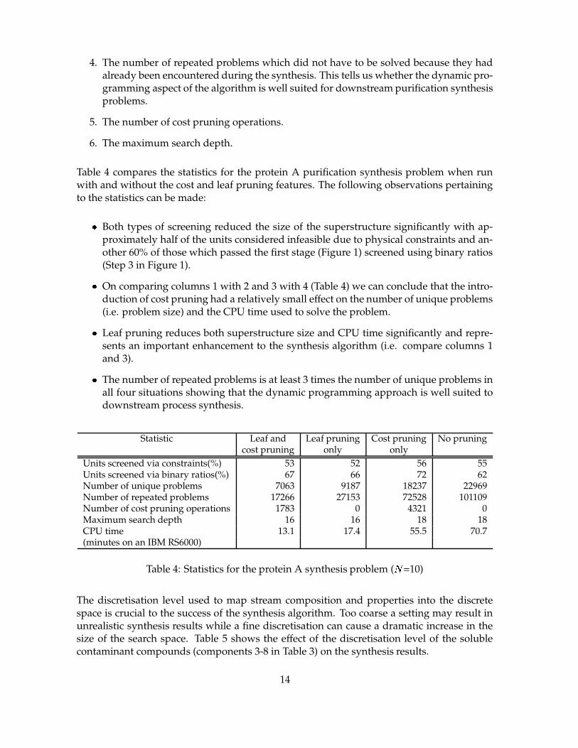
Table 4 compares the statistics for the protein A purification synthesis problem when runwith and without the cost and leaf pruning features. The following observations pertainingto the statistics can be made:

� Both types of screening reduced the size of the superstructure significantly with ap-proximately half of the units considered infeasible due to physical constraints and an-other 60% of those which passed the first stage (Figure 1) screened using binary ratios(Step 3 in Figure 1).

� On comparing columns 1 with 2 and 3 with 4 (Table 4) we can conclude that the intro-duction of cost pruning had a relatively small effect on the number of unique problems(i.e. problem size) and the CPU time used to solve the problem.

� Leaf pruning reduces both superstructure size and CPU time significantly and repre-sents an important enhancement to the synthesis algorithm (i.e. compare columns 1and 3).

� The number of repeated problems is at least 3 times the number of unique problems inall four situations showing that the dynamic programming approach is well suited todownstream process synthesis.

Statistic Leaf and Leaf pruning Cost pruning No pruningcost pruning only only

Units screened via constraints(%) 53 52 56 55Units screened via binary ratios(%) 67 66 72 62Number of unique problems 7063 9187 18237 22969Number of repeated problems 17266 27153 72528 101109Number of cost pruning operations 1783 0 4321 0Maximum search depth 16 16 18 18CPU time 13.1 17.4 55.5 70.7(minutes on an IBM RS6000)

Table 4: Statistics for the protein A synthesis problem ( t =10)

The discretisation level used to map stream composition and properties into the discretespace is crucial to the success of the synthesis algorithm. Too coarse a setting may result inunrealistic synthesis results while a fine discretisation can cause a dramatic increase in thesize of the search space. Table 5 shows the effect of the discretisation level of the solublecontaminant compounds (components 3-8 in Table 3) on the synthesis results.

14

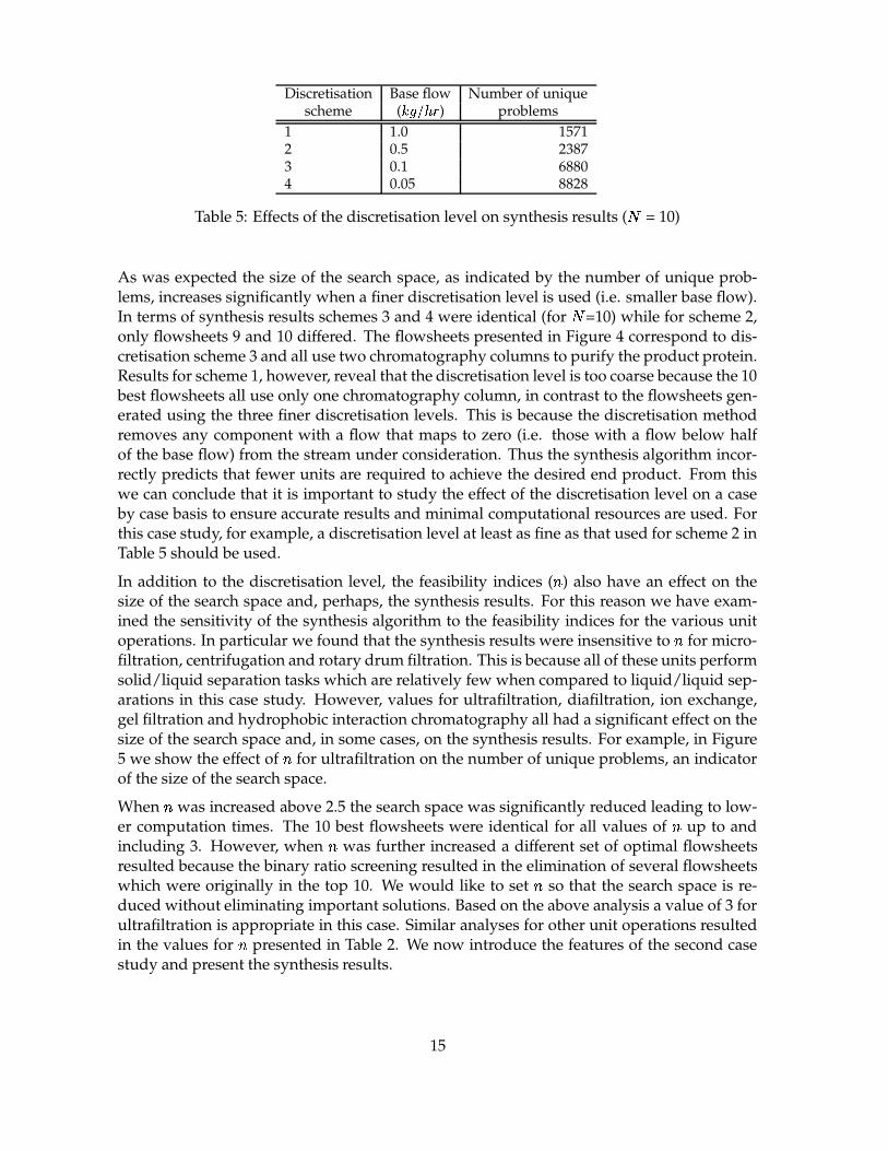
Discretisation Base flow Number of uniquescheme ( _� �"�`�a ) problems

1 1.0 15712 0.5 23873 0.1 68804 0.05 8828

Table 5: Effects of the discretisation level on synthesis results ( t = 10)

As was expected the size of the search space, as indicated by the number of unique prob-lems, increases significantly when a finer discretisation level is used (i.e. smaller base flow).In terms of synthesis results schemes 3 and 4 were identical (for t =10) while for scheme 2,only flowsheets 9 and 10 differed. The flowsheets presented in Figure 4 correspond to dis-cretisation scheme 3 and all use two chromatography columns to purify the product protein.Results for scheme 1, however, reveal that the discretisation level is too coarse because the 10best flowsheets all use only one chromatography column, in contrast to the flowsheets gen-erated using the three finer discretisation levels. This is because the discretisation methodremoves any component with a flow that maps to zero (i.e. those with a flow below halfof the base flow) from the stream under consideration. Thus the synthesis algorithm incor-rectly predicts that fewer units are required to achieve the desired end product. From thiswe can conclude that it is important to study the effect of the discretisation level on a caseby case basis to ensure accurate results and minimal computational resources are used. Forthis case study, for example, a discretisation level at least as fine as that used for scheme 2 inTable 5 should be used.

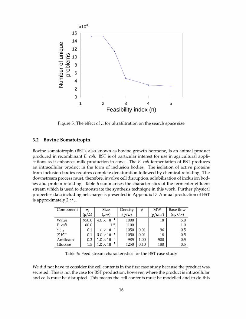
In addition to the discretisation level, the feasibility indices ( A ) also have an effect on thesize of the search space and, perhaps, the synthesis results. For this reason we have exam-ined the sensitivity of the synthesis algorithm to the feasibility indices for the various unitoperations. In particular we found that the synthesis results were insensitive to A for micro-filtration, centrifugation and rotary drum filtration. This is because all of these units performsolid/liquid separation tasks which are relatively few when compared to liquid/liquid sep-arations in this case study. However, values for ultrafiltration, diafiltration, ion exchange,gel filtration and hydrophobic interaction chromatography all had a significant effect on thesize of the search space and, in some cases, on the synthesis results. For example, in Figure5 we show the effect of A for ultrafiltration on the number of unique problems, an indicatorof the size of the search space.

When A was increased above 2.5 the search space was significantly reduced leading to low-er computation times. The 10 best flowsheets were identical for all values of A up to andincluding 3. However, when A was further increased a different set of optimal flowsheetsresulted because the binary ratio screening resulted in the elimination of several flowsheetswhich were originally in the top 10. We would like to set A so that the search space is re-duced without eliminating important solutions. Based on the above analysis a value of 3 forultrafiltration is appropriate in this case. Similar analyses for other unit operations resultedin the values for A presented in Table 2. We now introduce the features of the second casestudy and present the synthesis results.

15

0

2

4

6

8

10

12

14

16

1 2 3 4 5

Feasibility index (n)

Num

ber

of u

niqu

e pr

oble

ms

x103

Figure 5: The effect of A for ultrafiltration on the search space size

3.2 Bovine Somatotropin

Bovine somatotropin (BST), also known as bovine growth hormone, is an animal productproduced in recombinant E. coli. BST is of particular interest for use in agricultural appli-cations as it enhances milk production in cows. The E. coli fermentation of BST producesan intracellular product in the form of inclusion bodies. The isolation of active proteinsfrom inclusion bodies requires complete denaturation followed by chemical refolding. Thedownstream process must, therefore, involve cell disruption, solubilisation of inclusion bod-ies and protein refolding. Table 6 summarises the characteristics of the fermenter effluentstream which is used to demonstrate the synthesis technique in this work. Further physicalproperties data including net charge is presented in Appendix D. Annual production of BSTis approximately 2 P � Y .

Component � Z Size Density [ MW Base flow( +"\# ) ( � ) ( �"!# ) ( �"\�u]\^ ) ( _� �"�`�a )

Water 950.0 0 � ��bi�(��d�e 1000 18 5.0E. coli 60.0 1.5 1100 1.0fvg de 0.1 �2� ��bc����dop 1050 0.01 96 0.5jmk le 0.1 ' � ��bc����d�e 1050 0.01 18 0.5Antifoam 0.3 ��� ��bc����dw 985 1.00 500 0.5Glucose 1.5 ��� ��bc����dop 1250 0.10 180 0.5

Table 6: Feed stream characteristics for the BST case study

We did not have to consider the cell contents in the first case study because the product wassecreted. This is not the case for BST production, however, where the product is intracellularand cells must be disrupted. This means the cell contents must be modelled and to do this

16

we make several simplifying assumptions:

� Cells are assumed to contain 13 dissolved proteins along with the inclusion bodies.These proteins were identified as the most abundant, apart from the product, in atypical E. coli cell and were subsequently characterised in work presented by Leseret al. (1996). Data for all biochemicals also include a titration curve (i.e. charge as afunction of pH) which is used for ion exchange chromatography selection and design(Appendix E).

� Inclusion bodies are assumed to contain 50% BST with the remainder approximated asa single contaminating protein (Appendix D).

� Cell debris is assumed to consist of cell wall material only and the average particle sizeis specified as part of the homogeniser design procedure (Appendix A).

The composition and physical properties of the E. coli cells used for this case study is pre-sented in Table 7.

Component % w/w x (g/L) Size ( � ) Base Flow ( _: +"!`+a )Water 70 1000 0 � �ybi�(��d�eCell wall material 7 1150 0.65Soluble proteins 18 1300 Appendix EInclusion bodies 5 1270 0.4

Table 7: E. coli cell composition for the BST case study

Eleven different unit operations were considered in the synthesis procedure including: mi-crofiltration, centrifugation, ultrafiltration, diafiltration, rotary drum filtration, homogenisa-tion, denature/refolding tanks, cation exchange, anion exchange, hydrophobic interactionchromatography and gel filtration. Feasibility indices used for this case study were present-ed in Table 2. In addition we have defined two terminating units: a product tank whichaccepts streams containing BST at the desired concentration (300

��:r) and purity (99.9%)

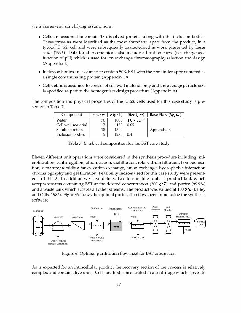
and a waste tank which accepts all other streams. The product was valued at 100s ���

(Baileyand Ollis, 1986). Figure 6 shows the optimal purification flowsheet found using the synthesissoftware.

Fermentor

Homogeniser

Refolding tank Anion

exchanger Gel

filtration

Ultrafilter (concentration)

Product Tank

Centrifuge

Diafiltration Concentration and Diafiltration

Water + soluble medium components

Water + soluble cell contents

Water + urea

Urea

Water

Water Water

Figure 6: Optimal purification flowsheet for BST production

As is expected for an intracellular product the recovery section of the process is relativelycomplex and contains five units. Cells are first concentrated in a centrifuge which serves to

17

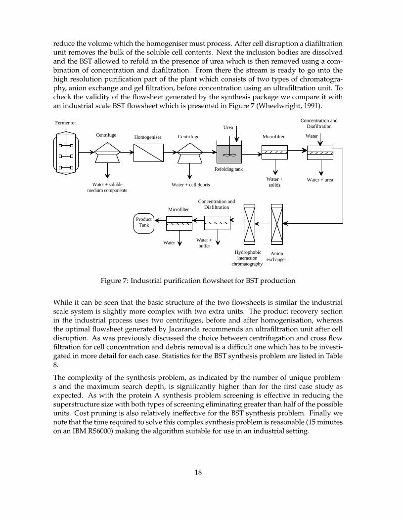
reduce the volume which the homogeniser must process. After cell disruption a diafiltrationunit removes the bulk of the soluble cell contents. Next the inclusion bodies are dissolvedand the BST allowed to refold in the presence of urea which is then removed using a com-bination of concentration and diafiltration. From there the stream is ready to go into thehigh resolution purification part of the plant which consists of two types of chromatogra-phy, anion exchange and gel filtration, before concentration using an ultrafiltration unit. Tocheck the validity of the flowsheet generated by the synthesis package we compare it withan industrial scale BST flowsheet which is presented in Figure 7 (Wheelwright, 1991).

Fermentor

Homogeniser

Refolding tank

Anion exchanger

Hydrophobic interaction

chromatography

Product Tank

Centrifuge

Concentration and Diafiltration

Water + soluble medium components

Water + urea

Urea

Water + buffer

Water

Water + cell debris

Centrifuge

Water + solids

Microfilter

Concentration and Diafiltration

Water

Microfilter

Figure 7: Industrial purification flowsheet for BST production

While it can be seen that the basic structure of the two flowsheets is similar the industrialscale system is slightly more complex with two extra units. The product recovery sectionin the industrial process uses two centrifuges, before and after homogenisation, whereasthe optimal flowsheet generated by Jacaranda recommends an ultrafiltration unit after celldisruption. As was previously discussed the choice between centrifugation and cross flowfiltration for cell concentration and debris removal is a difficult one which has to be investi-gated in more detail for each case. Statistics for the BST synthesis problem are listed in Table8.

The complexity of the synthesis problem, as indicated by the number of unique problem-s and the maximum search depth, is significantly higher than for the first case study asexpected. As with the protein A synthesis problem screening is effective in reducing thesuperstructure size with both types of screening eliminating greater than half of the possibleunits. Cost pruning is also relatively ineffective for the BST synthesis problem. Finally wenote that the time required to solve this complex synthesis problem is reasonable (15 minuteson an IBM RS6000) making the algorithm suitable for use in an industrial setting.

18

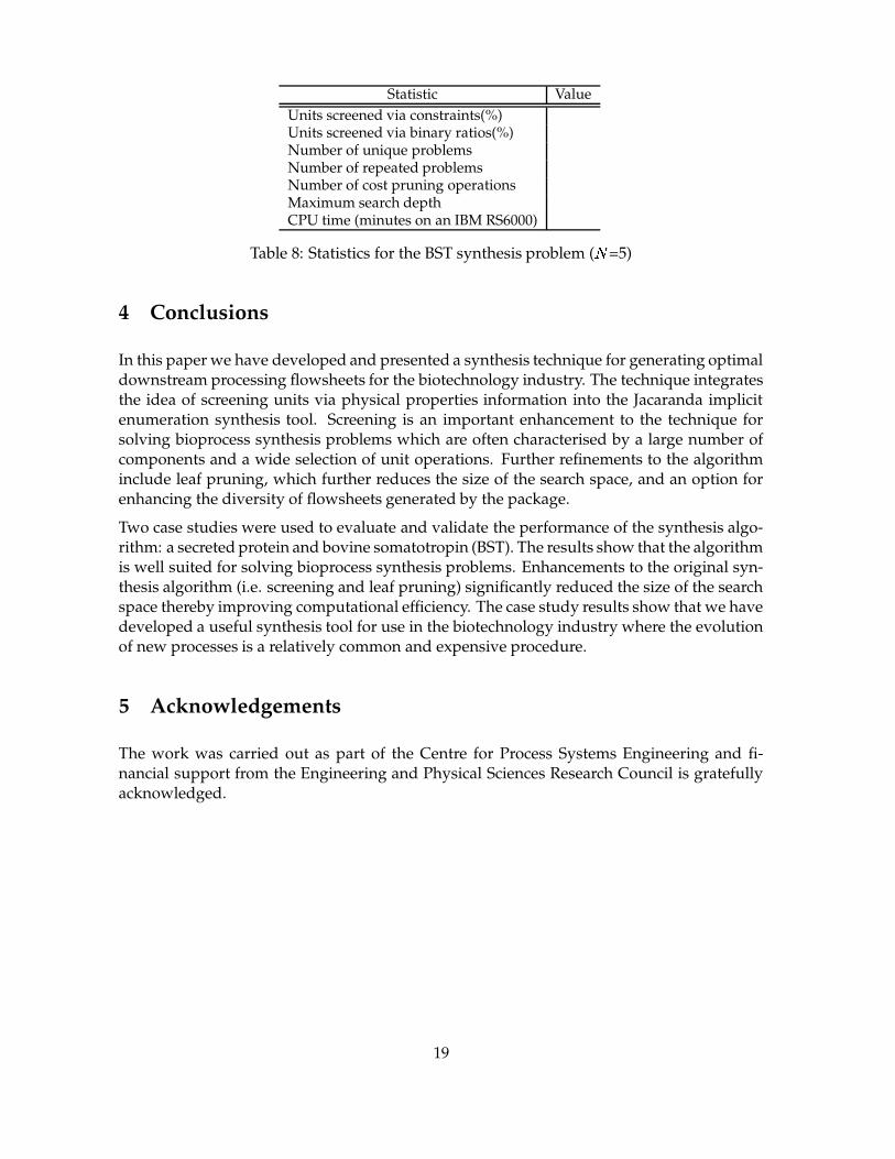
Statistic ValueUnits screened via constraints(%)Units screened via binary ratios(%)Number of unique problemsNumber of repeated problemsNumber of cost pruning operationsMaximum search depthCPU time (minutes on an IBM RS6000)

Table 8: Statistics for the BST synthesis problem ( t =5)

4 Conclusions

In this paper we have developed and presented a synthesis technique for generating optimaldownstream processing flowsheets for the biotechnology industry. The technique integratesthe idea of screening units via physical properties information into the Jacaranda implicitenumeration synthesis tool. Screening is an important enhancement to the technique forsolving bioprocess synthesis problems which are often characterised by a large number ofcomponents and a wide selection of unit operations. Further refinements to the algorithminclude leaf pruning, which further reduces the size of the search space, and an option forenhancing the diversity of flowsheets generated by the package.

Two case studies were used to evaluate and validate the performance of the synthesis algo-rithm: a secreted protein and bovine somatotropin (BST). The results show that the algorithmis well suited for solving bioprocess synthesis problems. Enhancements to the original syn-thesis algorithm (i.e. screening and leaf pruning) significantly reduced the size of the searchspace thereby improving computational efficiency. The case study results show that we havedeveloped a useful synthesis tool for use in the biotechnology industry where the evolutionof new processes is a relatively common and expensive procedure.

5 Acknowledgements

The work was carried out as part of the Centre for Process Systems Engineering and fi-nancial support from the Engineering and Physical Sciences Research Council is gratefullyacknowledged.

19

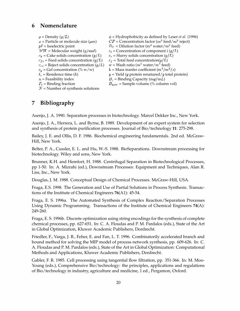
6 Nomenclature

x = Density ( �"!# ) [ = Hydrophobicity as defined by Leser et al. (1996)� = Particle or molecule size ( � ) z&{ = Concentration factor ( � p feed/ � p reject)|�} = Isoelectric point ~�� = Dilution factor ( �Op water/ �Op feed)���

= Molecular weight ( �"\�u]\^ ) � Z = Concentration of component i ( �"!# )��� = Cake solids concentration ( +"\# ) ��- = Slurry solids concentration ( +"\# )���1- = Feed solids concentration ( �"!# ) ��� = Total feed concentration( �"!# )�%$.- = Reject solids concentration ( �"!# ) ; = Wash ratio ( �4p water/ �Op feed)��� = Gel concentration (% w/w) k = Mass tranfer coefficient ( ��p�"1�On("�� )� $ = Residence time ( ` ) � = Yield ( protein renatured/ total protein)@ = Feasibility index �&� = Binding Capacity ( �� �"\�u# ){ Z = Binding fraction � -���� = Sample volume (% column vol)j = Number of synthesis solutions

7 Bibliography

Asenjo, J. A. 1990. Separation processes in biotechnology. Marcel Dekker Inc., New York.

Asenjo, J. A., Herrera, L. and Byrne, B. 1989. Development of an expert system for selectionand synthesis of protein purification processes. Journal of Bio/technology 11: 275-298.

Bailey, J. E. and Ollis, D. F. 1986. Biochemical engineering fundamentals. 2nd ed. McGraw-Hill, New York.

Belter, P. A., Cussler, E. L. and Hu, W.-S. 1988. BioSeparations. Downstream processing forbiotechnology. Wiley and sons, New York.

Brunner, K.H. and Hemfort, H. 1988. Centrifugal Separation in Biotechnological Processes,pp 1-50. In: A. Mizrahi (ed.), Downstream Processes: Equipment and Techniques, Alan R.Liss, Inc., New York.

Douglas, J. M. 1988. Conceptual Design of Chemical Processes. McGraw-Hill, USA.

Fraga, E.S. 1998. The Generation and Use of Partial Solutions in Process Synthesis. Transac-tions of the Institute of Chemical Engineers 76(A1): 45-54.

Fraga, E. S. 1996a. The Automated Synthesis of Complex Reaction/Separation ProcessesUsing Dynamic Programming. Transactions of the Institute of Chemical Engineers 74(A):249-260.

Fraga, E. S. 1996b. Discrete optimization using string encodings for the synthesis of completechemical processes, pp. 627-651. In: C. A. Floudas and P. M. Pardalos (eds.), State of the Artin Global Optimization, Kluwer Academic Publishers, Dordrecht.

Friedler, F., Varga, J. B., Feher, E. and Fan, L. T. 1996. Combinatorily accelerated branch andbound method for solving the MIP model of process network synthesis, pp. 609-626. In: C.A. Floudas and P. M. Pardalos (eds.), State of the Art in Global Optimization: ComputationalMethods and Applications, Kluwer Academic Publishers, Dordrecht.

Gabler, F. R. 1985. Cell processing using tangential flow filtration, pp. 351-366. In: M. Moo-Young (eds.), Comprehensive Bio/technology: the principles, applications and regulationsof Bio/technology in industry, agriculture and medicine, 1 ed., Pergamon, Oxford.

20

Grossman, I. E. and Kravanja, Z. 1995. Mixed Integer Non-linear Programming Techniquesfor Process Systems Engineering. Computers and chemical engineering 19(Suppl.): S83-S88.

Ho, W. S. and Sirkar, K. S. 1992. Membrane Handbook. 1st ed. Van Nostrand Reinhold, NewYork.

Intelligen, Inc. 1997. BioPro Designer User Guide.

Jaksland, C. A., Gani, R. and Lien, K. M. 1995. Separation process design and synthesis basedon thermodynamic insights. Chemical engineering science 50(3): 511-530.

Kennedy, J. F. and Cabral, J. M. S. 1993. Recovery Processes for Biological Materials. JohnWiley and Sons, Chichester.

Klein, B. K., Hill, S. R., Devine, C. S., Rowold, E., Smith, C. E., Galosy, S. and Olins, P. O.1991. Secretion of active bovine somatotropin in Esherischia coli. Bio/technology 9: 869-872.

Leser, E. W. and Asenjo, J. A. 1992. Rational Design of Purification Processes For Recombi-nant Proteins. Journal of Chromatography-Biomedical Applications 584(1): 43-57.

Leser, E. W., Lienqueo, M. E. and Asenjo, J. A. 1996. Implementation in an Expert-Systemof a Selection Rationale For Purification Processes For Recombinant Proteins. Annals of theNew York Academy of Sciences 782: 441-455.

Lienqueo, M. E., Leser, E. W. and Asenjo, J. A. 1996. An Expert-System For the Selection andSynthesis of Multistep Protein Separation Processes. Computers and Chemical Engineering20(SA): S 189-S 194.

Nilsson, B. 1990. Fusions to Staphylococcal protein A. Methods in Enzymology 185: 144.

Peters, M. S. and Timmerhaus, K. D. 1991. Plant design and economics for chemical engi-neers. 4th ed. McGraw Hill, New York.

Petrides, D. P. 1994. Biopro Designer - an Advanced Computing Environment For Model-ing and Design of Integrated Biochemical Processes. Computers and Chemical Engineering18(SS): S621-S625.

Petrides, D. P., Calandranis, J. and Cooney, C. 1995. Computer-Aided-Design TechniquesFor Integrated Biochemical Processes. Genetic Engineering News 15(16): 10.

Reisman, H. 1988. Economic analysis of fermentation processes. CRC Press, Boca Raton.

Smith, E. M. and Pantelides, C. C. 1995. Design of Reaction/Separation networks usingdetailed models. Computers and chemical engineering 19(Suppl.): S83-S88.

Steffens, M. A., Fraga, E. S. and Bogle, I. D. L. 1999. Optimal System Wide Design for Biopro-cesses. Bioprocesses. To be presented at the 9th European Symposium on Computer Aided ProcessEngineering: ESCAPE-9, Budapest.

Tutunijian, R. S. 1985. Cell separations with holllow fiber membranes, pp. 367-381. In: M.Moo-Young (eds.), Comprehensive Bio/technology: the principles, applications and regula-tions of Bio/technology in industry, agriculture and medicine, 1 ed., Pergamon, Oxford.

Wheelwright, S. M. 1987. Designing downstream processes for large-scale protein purifica-tion. Bio/technology 5: 789.

Wheelwright, S. M. 1991. Protein purification: design and scale up of downstream process-ing. Hanser, Munich.

21

A Unit design parameters

Unit Parameter valuesUltrafilter E1F���������K � K� �3�����m�<�\�o��� �¢¡ � �¢£ ��¤

B¥C¦���o����� ¡ � � ¡Microfilter E1F��¨§��+��K � K� �3���©���<�\�o��ª �¢¡ � �¢£ ��¤

B¥C¦���o����� ¡ � � ¡Diafilter E1F���������K � K� �3�����m�<�\�o��� �¢¡ � �¢£ ��¤

G4H<��«o���y� ¡ � � ¡Centrifuge E!J¬�)�!��� ���:r

Bowl speed = 963¤ �®­

Number of discs = 72Disc opening angle = «�¯�°Inner diameter = 0.072 �Outer diameter = 0.162 �Dynamic viscosity = 1.02

���� � ¤Rotary drum filter E\LD��«�����K � K

K��3�������¢¡K�±�P�² +� �¢¡´³®²2²!µCake resistance = �o�����<�\� ­�­ � �����Pressure drop = ¶�¯ ��· ±Filtrate viscosity = ���������� ����� � ��¤Cycle time = �!¯�� ¤

Ion exchange Maximum diameter = 1.0 �chromatography PRQ = 5

�M�N = 20 � ��� �¢¸Column length = 0.25 �

Gel filtration Maximum diameter = 1.0 �M JTS%U = 5 %Column length = 0.5 �

Hydrophobic interaction Maximum diameter = 1.0 �chromatography MDN = 20 � ��� � r

P.Q = 5�

Column length = 0.25 �Homogenisation Cell debris size = 0.65 ¹®�

Recovery = 99 %

Solubilisation and P�Q = 44�

renaturing tank Y = 80 %Assume a solution of 3Mguanidine HCl is used

22

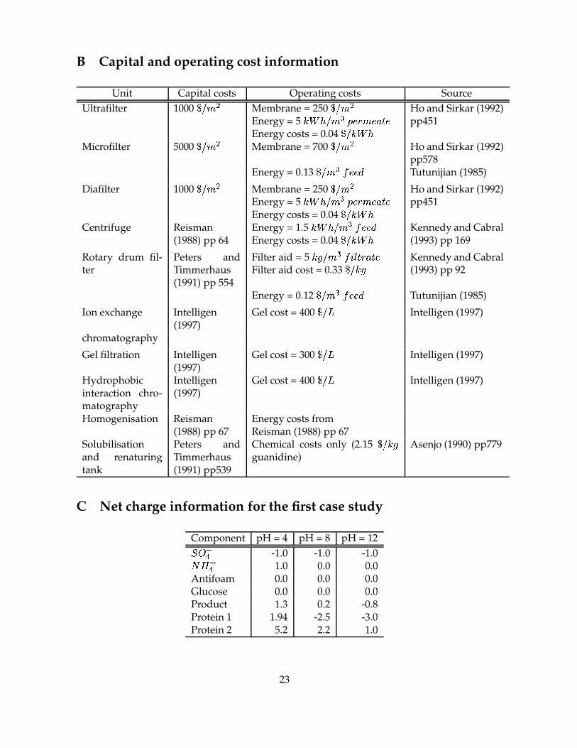
B Capital and operating cost information

Unit Capital costs Operating costs SourceUltrafilter 1000

s � � £ Membrane = 250s � � £

Energy = 5�»º¼�´� ��¡¾½¿² ��²�±+P�²

Energy costs = 0.04s ���»º��

Ho and Sirkar (1992)pp451

Microfilter 5000s � �*£ Membrane = 700

s � ��£ Ho and Sirkar (1992)pp578

Energy = 0.13s � � ¡ ³®²2²!µ Tutunijian (1985)

Diafilter 1000s � �*£ Membrane = 250

s � ��£Energy = 5

�»º¼�´� � ¡ ½¿² ��²�±+P�²Energy costs = 0.04

s ���»º��Ho and Sirkar (1992)pp451

Centrifuge Reisman(1988) pp 64

Energy = 1.5�»º��¿� ��¡ ³®²2²!µ

Energy costs = 0.04s ���»º�� Kennedy and Cabral

(1993) pp 169

Rotary drum fil-ter

Peters andTimmerhaus(1991) pp 554

Filter aid = 5����� ��¡/³¿ÀÁ¸ÂP ±�P�²

Filter aid cost = 0.33s ����� Kennedy and Cabral

(1993) pp 92

Energy = 0.12s � �*¡&³®²2²!µ Tutunijian (1985)

Ion exchange Intelligen(1997)

Gel cost = 400s �:r

Intelligen (1997)

chromatography

Gel filtration Intelligen(1997)

Gel cost = 300s �:r

Intelligen (1997)

Hydrophobicinteraction chro-matography

Intelligen(1997)

Gel cost = 400s �:r

Intelligen (1997)

Homogenisation Reisman(1988) pp 67

Energy costs fromReisman (1988) pp 67

Solubilisationand renaturingtank

Peters andTimmerhaus(1991) pp539

Chemical costs only (2.15s �����

guanidine)Asenjo (1990) pp779

C Net charge information for the first case study

Component pH = 4 pH = 8 pH = 12Ã6Ä �Å -1.0 -1.0 -1.0t�Æ=ÇÅ 1.0 0.0 0.0Antifoam 0.0 0.0 0.0Glucose 0.0 0.0 0.0Product 1.3 0.2 -0.8Protein 1 1.94 -2.5 -3.0Protein 2 5.2 2.2 1.0

23

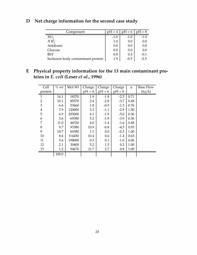
D Net charge information for the second case study

Component pH = 4 pH = 6 pH = 8Ã6Ä �Å -1.0 -1.0 -1.0t�Æ ÇÅ 1.0 0.0 0.0Antifoam 0.0 0.0 0.0Glucose 0.0 0.0 0.0BST 0.8 0.4 -0.1Inclusion body contaminant protein 1.9 -0.5 -2.5

E Physical property information for the 13 main contaminant pro-teins in E. coli (Leser et al., 1996)

Cell % wt Mol Wt Charge Charge Charge X Base Flowprotein pH = 4 pH = 6 pH = 8 (

�������)

1 16.1 18370 1.9 -1.8 -2.5 0.712 10.1 85570 2.4 -2.8 -3.7 0.483 6.6 53660 1.8 -0.5 -1.3 0.764 7.9 120000 3.3 -1.1 -2.9 1.505 6.9 203000 4.1 -1.9 -5.0 0.366 3.6 69380 5.2 -1.9 -3.9 0.367 11.0 48320 4.0 -1.4 -1.6 0.488 9.7 93380 10.9 -0.8 -4.5 0.939 10.7 69380 1.1 0.0 -0.3 1.0010 8.6 114450 10.4 0.6 -1.4 0.6311 5.6 198000 0.3 0.1 -1.0 0.0612 2.1 30400 5.2 1.5 0.2 1.0013 1.2 94670 11.7 2.7 0.8 1.00

100.0

24