MA 331 Intermediate MA 331 Intermediate StatisticsStatistics

Fall 2006Fall 2006

Webpage:Webpage:

http://www.math.stevens.edu/http://www.math.stevens.edu/~ifloresc/Teaching/2006-2007/~ifloresc/Teaching/2006-2007/

index331.htmlindex331.html

Instructor : Ionut FlorescuInstructor : Ionut Florescu OfficeOffice: Kidde 227 Phone 201-216-5452: Kidde 227 Phone 201-216-5452 Office hoursOffice hours: TTh 11:00-12:00, or by : TTh 11:00-12:00, or by

appointment.appointment. Please print off the course information Please print off the course information

posted on web.posted on web. EmailEmail:: ifloresc@stevens.eduifloresc@stevens.edu MailboxMailbox: in Math. Dept office.: in Math. Dept office.

GradesGrades

Homework (30%) – almost every week, Homework (30%) – almost every week, usually due on Thursdays. usually due on Thursdays.

Quizzes and attendance (10%) – there will Quizzes and attendance (10%) – there will be a few quizzes given during the course be a few quizzes given during the course of the semester. Attendance is not of the semester. Attendance is not mandatory, however if you get into the mandatory, however if you get into the habit of skipping the lecture I will deduct habit of skipping the lecture I will deduct points. Participation in the lecture is points. Participation in the lecture is rewarded here as well.rewarded here as well.

Final exam (30%) – during the finals week, Final exam (30%) – during the finals week, closed books/notes.closed books/notes.

Grades (cont.)Grades (cont.) Project (30%) There are two parts of the Project (30%) There are two parts of the

project. The students are supposed to work project. The students are supposed to work in groups of maximum 4.in groups of maximum 4.

For the first part of the project you will be For the first part of the project you will be required to find an interesting dataset required to find an interesting dataset suitable for analysis. You will write a proposal suitable for analysis. You will write a proposal detailing a description and interesting detailing a description and interesting features of the dataset, questions that would features of the dataset, questions that would be useful to answer, and proposed methods.be useful to answer, and proposed methods.

For the second part of the project you will For the second part of the project you will implement methods learned in class to implement methods learned in class to analyze the dataset from the first part of the analyze the dataset from the first part of the project.project.

Grades (cont.)Grades (cont.)

You should assume regular cutoffs You should assume regular cutoffs (90%-100% A etc.), however depending (90%-100% A etc.), however depending on the performance of the class the on the performance of the class the final percentages may be curved.final percentages may be curved.

R is needed for the class. You will need R is needed for the class. You will need to use it for the project and homework to use it for the project and homework problems and I may test your problems and I may test your knowledge of R in the exam and knowledge of R in the exam and quizzes.quizzes.

TextbooksTextbooks

Introduction to the Practice of Introduction to the Practice of StatisticsStatistics, , 4th edition4th edition, by David S. , by David S. Moore and George P. McCabe.Moore and George P. McCabe.

Introductory Statistics with R, Introductory Statistics with R, by by Peter Dalgaard.Peter Dalgaard.

Data, Data, Data, all around us !Data, Data, Data, all around us !

We use data to answer research We use data to answer research questionsquestions

What evidence does data provide?What evidence does data provide?Example 1:Example 1:Subject SBP HR BG Age Weight TreatmentSubject SBP HR BG Age Weight Treatment11 120 84 100 45 140 1120 84 100 45 140 122 160 75 233 52 160 1160 75 233 52 160 133 95 63 92 44 110 295 63 92 44 110 2. . . . . . .. . . . . . .

How do I make sense of these How do I make sense of these numbers without some meaningful numbers without some meaningful summary?summary?

Example 2Example 2

Study to assess the effect of exercise on Study to assess the effect of exercise on cholesterol levels. One group exercises and cholesterol levels. One group exercises and other does not. Is cholesterol reduced in other does not. Is cholesterol reduced in exercise group?exercise group? people have naturally different levelspeople have naturally different levels respond differently to same amount of respond differently to same amount of

exercise (e.g. genetics)exercise (e.g. genetics) may vary in adherence to exercise regimenmay vary in adherence to exercise regimen diet may have an effectdiet may have an effect exercise may affect other factors (e.g. exercise may affect other factors (e.g.

appetite, energy, schedule)appetite, energy, schedule)

What is statistics?What is statistics?

• Recognize the randomness, the Recognize the randomness, the variability in data.variability in data.

• ““the science of understanding data the science of understanding data and making decisions in face of and making decisions in face of variability”variability”

• Design the studyDesign the study• Analyze the collected Data Analyze the collected Data **• Discover what data is telling you…Discover what data is telling you…

Structure of the courseStructure of the course Part I: Data:Part I: Data:

Analysis and productionAnalysis and production Examine, organize and summarizeExamine, organize and summarize Basic data analysisBasic data analysis Preliminary descriptive statisticsPreliminary descriptive statistics

Part II: Statistical InferencePart II: Statistical Inference Introduction to probability conceptsIntroduction to probability concepts Formal Method of drawing conclusionsFormal Method of drawing conclusions Formal Statistical TestsFormal Statistical Tests Testing the reliability of conclusionsTesting the reliability of conclusions

Part III: Advanced Statistical InferencePart III: Advanced Statistical Inference Analyzing relationships between 2 or more variables Analyzing relationships between 2 or more variables

Chapter 1Chapter 1 IndividualsIndividuals – objects described by a set of data – objects described by a set of data

(people, animals, things)(people, animals, things) VariableVariable – characteristic of an individual, takes – characteristic of an individual, takes

different values for different subjects.different values for different subjects. The three questions to ask : The three questions to ask :

Why: Purpose of study?Why: Purpose of study? Who: Members of the sample, how many?Who: Members of the sample, how many? What: What did we measure (the variables) and in What: What did we measure (the variables) and in

what units?what units? Example: Example:

In a study on how the In a study on how the time spent partyingtime spent partying affects the affects the GPAGPA variables like variables like ageage, , student’s majorstudent’s major, , heightheight, , weightweight were also recorded… were also recorded…

Variable types:Variable types:

Categorical Categorical – outcomes fall into – outcomes fall into categoriescategories

QuantitativeQuantitative – outcome is a number – outcome is a number ContinuousContinuous : height, weight, distance : height, weight, distance

Can take any value within a rangeCan take any value within a range Discrete Discrete : number of phone calls made every : number of phone calls made every

week, number of accidents on SR 26, number week, number of accidents on SR 26, number of students getting A in Stat 501 this Fallof students getting A in Stat 501 this Fall

Can not take all possible values (integers here)Can not take all possible values (integers here) Arithmetic operations like addition subtraction, etc. Arithmetic operations like addition subtraction, etc.

are meaningfulare meaningful

Information on employees of CyberStat

Distribution of a variable:Distribution of a variable:

What values a variable takesWhat values a variable takes How often the variable takes those values How often the variable takes those values

(frequency)(frequency)

Preliminary Analysis of Variables and Preliminary Analysis of Variables and their distributions:their distributions: Display variables graphically (with pictures)Display variables graphically (with pictures) Basic Descriptive Statistics (with numbers)Basic Descriptive Statistics (with numbers)

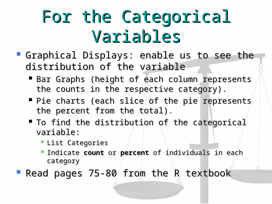
For the Categorical VariablesFor the Categorical Variables

Graphical Displays: enable us to see the Graphical Displays: enable us to see the distribution of the variabledistribution of the variable Bar Graphs (height of each column represents the Bar Graphs (height of each column represents the

counts in the respective category).counts in the respective category). Pie charts (each slice of the pie represents the Pie charts (each slice of the pie represents the

percent from the total).percent from the total). To find the distribution of the categorical variable:To find the distribution of the categorical variable:

List CategoriesList Categories Indicate Indicate countcount or or percentpercent of individuals in each of individuals in each

categorycategory

Read pages 75-80 from the R textbookRead pages 75-80 from the R textbook

Bar GraphBar Graph

Pie ChartPie Chart

ExerciseExercise

Example:Example:You are interested in studying the You are interested in studying the

distribution of various majors of 400 distribution of various majors of 400 students enrolled in an undergraduate students enrolled in an undergraduate program at a small university.program at a small university.

The following data is provided for you:The following data is provided for you: MajorMajor Number of StudentsNumber of Students Percent of Percent of

StudentsStudents MathMath 6565

16.25%16.25% StatStat 2020 5%5% EngineeringEngineering 250250 62.5%62.5% Health SciencesHealth Sciences 6565 16.25%16.25%

Quantitative Variables-Graphical Quantitative Variables-Graphical DisplayDisplay

Deviations from 24,800 nanoseconds

66 observations taken in July-Sept, 66 observations taken in July-Sept, 18821882

Variable: passage time, scaled and Variable: passage time, scaled and centered. centered.

Individual observations are different Individual observations are different since the environment of every since the environment of every measurement is slightly differentmeasurement is slightly different

We will examine the nature of the We will examine the nature of the variation of the quantitative variable variation of the quantitative variable by drawing graphsby drawing graphs

Graphical tools for quantitative dataGraphical tools for quantitative data

Stemplots Stemplots HistogramsHistograms

The stemplot is a simple version of the histogram used for The stemplot is a simple version of the histogram used for small datasets, that can be done by hand. small datasets, that can be done by hand.

Steps to construct a stemplot:Steps to construct a stemplot: Separate the value for each observation into the Separate the value for each observation into the stem stem and and

the the leafleaf.. The leaf is the final digit and the stem is made of all the The leaf is the final digit and the stem is made of all the

other digits.other digits. Write stems in a vertical column ordered.Write stems in a vertical column ordered. Write the smallest on the top and draw a vertical line to the Write the smallest on the top and draw a vertical line to the

right of the column.right of the column. Write each leaf next to the corresponding stemWrite each leaf next to the corresponding stem Write them increasingly from the stemWrite them increasingly from the stem

Stemplot exampleStemplot example

Example 1.4 Example 1.4 Numbers of home runs that Babe Ruth hit in each of Numbers of home runs that Babe Ruth hit in each of

his 15 years with the New York Yankees:his 15 years with the New York Yankees:54 59 35 41 46 25 47 60 54 46 49 46 41 34 2254 59 35 41 46 25 47 60 54 46 49 46 41 34 22 Step 1: Sort the data, sort the stems.Step 1: Sort the data, sort the stems.2 3 4 5 62 3 4 5 6 Step 2: Write the stems in increasing orderStep 2: Write the stems in increasing order22334 4 5566

Write the leaves against the stem in Write the leaves against the stem in increasing orderincreasing order

2 2 52 2 5

3 4 5 3 4 5

4 1 1 6 6 6 7 94 1 1 6 6 6 7 9

5 4 4 95 4 4 9

6 06 0

Back-to-back stemplotBack-to-back stemplot

Compare the numbers of Babe Ruth Compare the numbers of Babe Ruth hits and Mark McGwire hitshits and Mark McGwire hits

9 9 22 29 32 32 33 39 39 42 49 52 9 9 22 29 32 32 33 39 39 42 49 52 58 65 7058 65 70

0 9 90 9 9 11 5 2 2 2 95 2 2 2 9 5 4 3 2 2 3 9 9 5 4 3 2 2 3 9 9 9 7 6 6 6 1 1 4 2 99 7 6 6 6 1 1 4 2 9 9 4 4 5 2 89 4 4 5 2 8 0 6 50 6 5 7 07 0

Histograms (example)Histograms (example)

Histogram (cont)Histogram (cont) Within any set of numbers, a range exists Within any set of numbers, a range exists

where the variable takes on different values.where the variable takes on different values. Range = Maximum Value – Minimum ValueRange = Maximum Value – Minimum Value

Steps to constructing a histogram:Steps to constructing a histogram: Order dataOrder data Divide data into intervals (classes) of equal widthDivide data into intervals (classes) of equal width To choose interval width: Look to the range of the To choose interval width: Look to the range of the

data (from the minimum value to the maximum data (from the minimum value to the maximum value) and decide on how big the width should be value) and decide on how big the width should be so you would have about 5 to 9 classesso you would have about 5 to 9 classes

Count the number of observations in each Count the number of observations in each interval (class)interval (class)

GraphGraph

Frequency TableFrequency Table

ClassClass CountCount PercePercentnt

ClassClass CountCount PercePercentnt

0.1-5.00.1-5.0 3030 6060 20.1-2520.1-25 11 22

5.1-5.1-10.010.0

1010 2020 25.1-3025.1-30 22 44

10.1-1510.1-15 44 88 30.1-3530.1-35 00 00

15.1-2015.1-20 22 44 35.1-4035.1-40 11 22

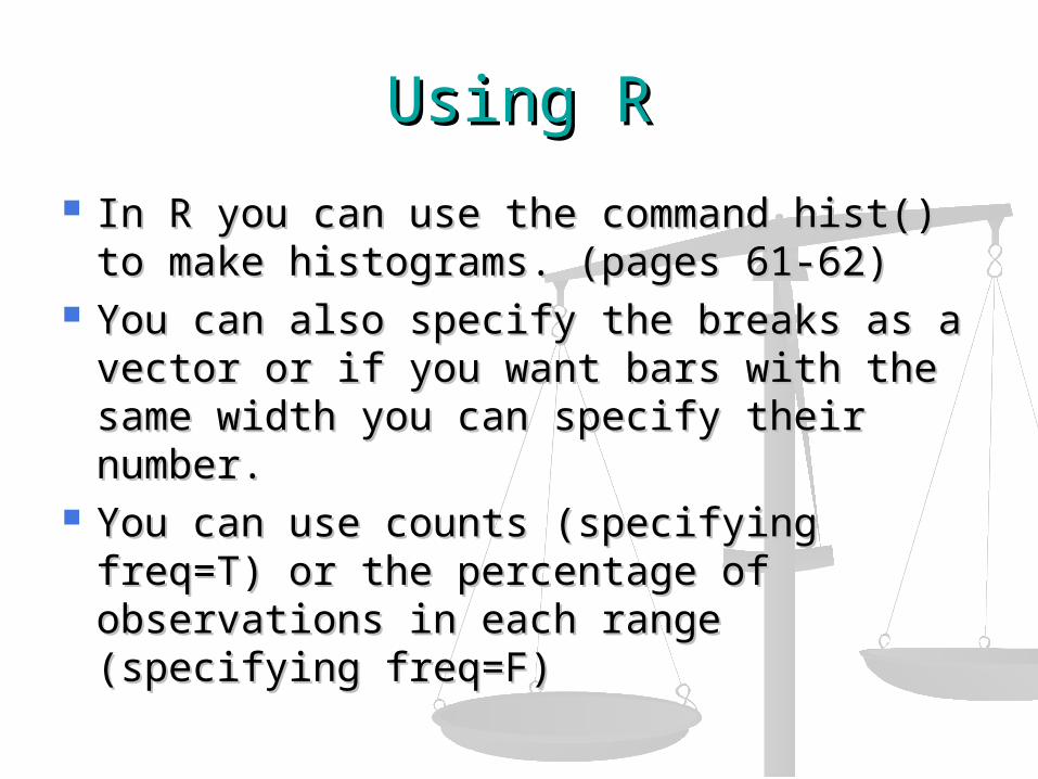
Using RUsing R

In R you can use the command hist() to In R you can use the command hist() to make histograms. (pages 61-62)make histograms. (pages 61-62)

You can also specify the breaks as a You can also specify the breaks as a vector or if you want bars with the same vector or if you want bars with the same width you can specify their number.width you can specify their number.

You can use counts (specifying freq=T) You can use counts (specifying freq=T) or the percentage of observations in or the percentage of observations in each range (specifying freq=F)each range (specifying freq=F)

Examining distributionsExamining distributions Describe the pattern – shape, center and Describe the pattern – shape, center and

spread.spread. Shape –Shape –

How many modes (peaks)?How many modes (peaks)? Symmetric or skewed in one direction (right tail Symmetric or skewed in one direction (right tail

longer or left)longer or left) Center – midpointCenter – midpoint Spread –range between the smallest and Spread –range between the smallest and

the largest values.the largest values. Look for outliers – individual values that do Look for outliers – individual values that do

not match the overall pattern.not match the overall pattern.

What do you see?What do you see?

Shape: Right skewed, unimodalShape: Right skewed, unimodal Center: about 5%Center: about 5% Spread : 0-40% with only one state Spread : 0-40% with only one state

more than 30%more than 30% Remember: Histograms only Remember: Histograms only

meaningful for quantitative datameaningful for quantitative data Is that extreme observation on the Is that extreme observation on the

right an outlier? right an outlier?

Newcomb’s data (dealing with Newcomb’s data (dealing with outliers)outliers)

OutliersOutliers

Check for recording errorsCheck for recording errors Violation of experimental conditionsViolation of experimental conditions Discard it only if there is a valid Discard it only if there is a valid

practical or statistical reason, not practical or statistical reason, not blindly!blindly!

Time plots. Newcomb’s data.

At the beginning much variationAt the beginning much variation Measurements stabilizing, less Measurements stabilizing, less

variation at a later time.variation at a later time.

Time seriesTime series

Plot observations over time (time on Plot observations over time (time on the x axis)the x axis)

Trend – persistent, long-term rise or fallTrend – persistent, long-term rise or fall Seasonal variation – a pattern that Seasonal variation – a pattern that

repeats itself at known regular intervals repeats itself at known regular intervals of time.of time.

Gasoline price data: Increasing trend, Gasoline price data: Increasing trend, small seasonal variations, increase in small seasonal variations, increase in spring and summer, slump in fall.spring and summer, slump in fall.

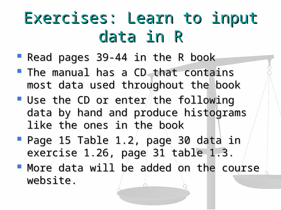
Exercises: Learn to input data in RExercises: Learn to input data in R

Read pages 39-44 in the R bookRead pages 39-44 in the R book The manual has a CD that contains most The manual has a CD that contains most

data used throughout the book data used throughout the book Use the CD or enter the following data by Use the CD or enter the following data by

hand and produce histograms like the hand and produce histograms like the ones in the bookones in the book

Page 15 Table 1.2, page 30 data in Page 15 Table 1.2, page 30 data in exercise 1.26, page 31 table 1.3.exercise 1.26, page 31 table 1.3.

More data will be added on the course More data will be added on the course website.website.

SummarySummary

Categorical and Quantitative variableCategorical and Quantitative variable Graphical tools for categorical Graphical tools for categorical

variablevariableBar Chart, Pie ChartBar Chart, Pie Chart For quantitative variable:For quantitative variable:Stem and leaf plot, histogramStem and leaf plot, histogram Describe: Shape, center, spreadDescribe: Shape, center, spread Watch out for patterns and Watch out for patterns and

deviations from patterns.deviations from patterns.