m5 east tunnels air quality monitoring project report july ... · south eastern sydney public...

SOUTH EASTERN SYDNEY PUBLIC HEALTH UNIT

& NSW DEPARTMENT OF HEALTH

M5 EAST TUNNELS AIR QUALITY

MONITORING PROJECT

REPORT JULY 2003

1

This report has been prepared by the investigators: Toni Cains, Santo Cannata, Kelly-Anne Ressler, Vicky Sheppeard and Mark Ferson

2

CONTENTS

LIST OF TABLES ............................................................................................4

LIST OF GRAPHS ...........................................................................................5

LIST OF FIGURES ..........................................................................................6

1. EXECUTIVE SUMMARY...........................................................................7

2. BACKGROUND.....................................................................................9 The M5 East Freeway ....................................................................... 9 Air Pollution ...................................................................................10 Carbon Monoxide............................................................................10 Particulate matter...........................................................................11 Nitrogen dioxide .............................................................................12 BTEX gases....................................................................................12 Benzene........................................................................................13 Toluene.........................................................................................13 Ethylbenzene .................................................................................13 Xylene ..........................................................................................13

3. THE STUDY ......................................................................................14 Aim/Objective ................................................................................14 Methodology ..................................................................................14

4. RESULTS .........................................................................................17 Transit Characteristics .....................................................................17 Cabin Carbon Monoxide ...................................................................19 External Carbon Monoxide ...............................................................21 Comparison with RTA CO monitors ....................................................22 Cabin Carbon Dioxide......................................................................24 External Carbon Dioxide ..................................................................26 PM2.5 - Dustrak ...............................................................................28 PM2.5 - Gravimetric ..........................................................................30 Cabin Nitrogen Dioxide ....................................................................31 External Nitrogen Dioxide ................................................................32 Benzene........................................................................................35 Toluene.........................................................................................36 Ethylbenzene .................................................................................37 Xylene ..........................................................................................38 Trends in pollutants ........................................................................39

5. DISCUSSION AND FINDINGS ................................................................43

6. ACKNOWLEDGMENTS ..........................................................................51

7. GLOSSARY .......................................................................................52

APPENDIX A: SUMMARY OF AIR QUALITY STANDARDS ........................................53

APPENDIX B: DAILY RECORD MONITORING SHEET .............................................54

APPENDIX C: CSIRO ANALYTICAL METHODS....................................................56

APPENDIX D: CALCULATIONS OF EXPOSURE INCREMENT FOR NON-THRESHOLD

POLLUTANTS ..............................................................................................56

REFERENCES ..............................................................................................65

3

LIST OF TABLES Table 1: Time taken (minutes) to traverse the tunnel for each trip direction during active sampling

Table 2: Average speed of the study vehicle compared with all traffic.

Table 3: RTA traffic statistics during study monitoring periods

Table 4: Trip averages for cabin CO by ventilation type (ppm)

Table 5: Trip averages for external CO (ppm) by trip direction

Table 6: Correlation between external CO and fixed monitors westbound afternoon.

Table 7: Correlation between external CO and fixed monitors eastbound afternoon.

Table 8: Trip averages for cabin CO2 (ppm) by ventilation type

Table 9: Trip averages for external CO2 (ppm) by trip direction

Table 10: Trip averages for cabin PM2.5 (µg/m3) Dustrak by ventilation type

Table 11: PM2.5 Gravimetric monitoring results

Table 12: Cabin NO2 levels (ppbv) by ventilation type

Table 13: Concentrations of BTEX gases (ppbv) including outlier

Table 14: Concentrations of BTEX gases (ppbv) excluding outlier

Table 15: Cabin benzene concentrations (ppbv) by ventilation type (including outlier)

Table 16: Cabin benzene concentrations (ppbv) by ventilation type (excluding outlier)

Table 17: Cabin toluene concentrations (ppbv) by ventilation type (including outlier)

Table 18: Cabin toluene concentrations (ppbv) by ventilation type (excluding outlier)

Table 19: Cabin ethylbenzene concentration (ppbv) by ventilation type (including outlier)

Table 20: Cabin ethylbenzene concentration (ppbv) by ventilation type (excluding outlier)

Table 21: Cabin xylene concentrations (ppbv) by ventilation type (including outlier)

Table 22: Cabin xylene concentrations (ppbv) by ventilation type (excluding outlier)

Table 23: Ratio of external pollutant levels to cabin pollutant levels by ventilation type

Table 24: PM2.5, CO and NO2 concentrations during the Sydney bushfires compared to the whole study period

4

LIST OF GRAPHS Graph 1: Trip averages for cabin CO ventilation type (ppm)

Graph 2: Averaged one-second cabin CO exposure (ppm) by time in tunnel

Graph 3: Trip averages for external CO (ppm) by trip direction

Graph 4: Averaged one-second external CO concentration (ppm) by time in tunnel

Graph 5: Trip averages for cabin CO2 (ppm) by ventilation type

Graph 6: Averaged one-second cabin CO2 exposure (ppm) by time in tunnel

Graph 7: Trip averages for external CO2 (ppm) by trip direction

Graph 8: Averaged one-second external CO2 concentration (ppm) by time in tunnel

Graph 9: Trip averages for cabin PM2.5 (µg/m3) by ventilation type

Graph 10: Averaged one-second cabin PM2.5 (µg/m3) exposure by time in tunnel

Graph 11: Cabin NO2 (ppbv) by ventilation type

Graph 12: Distribution of external NO2 (ppbv)

Graph 13: External NO2 versus cabin NO2 (when windows are closed)

Graph 14: Cabin benzene exposure (ppbv) by ventilation type

Graph 15: Cabin toluene exposure (ppbv) by ventilation type

Graph 16: Cabin ethylbenzene exposure (ppbv) by ventilation type

Graph 17: Cabin xylene exposure (ppbv) by ventilation type

Graph 18: Cabin PM2.5 Dustrak and CO Windows up, air conditioning on and recirculating

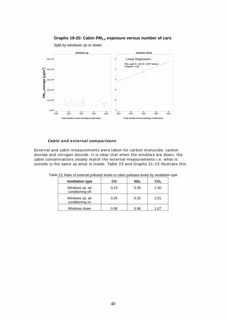
Graph 19-20: Cabin PM2.5 exposure versus number of cars split by windows up or down

Graph 21: Cabin (windows down) and external CO concentrations (ppm)

Graph 22: Cabin (windows down) and external CO2 concentrations (ppm)

Graph 23: Cabin (windows down) and external NO2 concentrations (ppbv)

Graph 24: Comparison of PM2.5 levels

Graph 25: Comparison of nitrogen dioxide levels

Graph 26: Comparison of carbon monoxide levels

Graph 27: Comparison of benzene levels

5

LIST OF FIGURES Figure 1: M5 East freeway tunnel ventilation system schematic

Figure 2: M5 East tunnel road grades

Figure 3: Penetration of particulate matter to the respiratory system

6

1. EXECUTIVE SUMMARY The effects of human exposure to air pollutants has been the subject of scientific research and government activity for several decades. Accumulating evidence demonstrates that exposure to air pollutants is associated with adverse health effects. Recently research has focussed on exposure in “micro environments” such as inside motor vehicles. Recent trends of population expansion, increased average vehicle kilometres travelled and increased vehicle ownership rates in cities such as Sydney, has resulted in over-congestion of surface roads. One response has been to build road tunnels. In December 2001, the M5 East freeway was opened to traffic and within six months in excess of 82,000 vehicles were using it daily. This freeway includes twin 4 kilometre tunnels (the longest in Australia), ventilated via a single exhaust stack. As it services major freight interchanges it carries a high proportion of trucks in comparison with other Sydney road tunnels. The combination of high usage (with higher truck numbers) and the ventilation characteristics of the tunnel mean that there is on occasion visible haze in the tunnels. A key health concern in managing the air quality in tunnels is exposure to carbon monoxide, which is controlled by tunnel ventilation. On a number of occasions since opening, incidents such as breakdowns and accidents have necessitated closure of a tunnel to ensure that motorists are not exposed to excessive levels of carbon monoxide. In response to community concerns regarding in-tunnel pollution levels we proposed this study to monitor pollutant levels in vehicles to the NSW Roads and Traffic Authority. The purpose of this study is to quantify exposure to several common motor vehicle pollutants during peak periods. We also wished to determine what impact vehicle ventilation has on pollutant levels. We collected carbon monoxide (CO), carbon dioxide and fine particles over 94 trips and nitrogen dioxide(NO2), BTEX gases and fine particles over 372 trips, during a six week period. Transit times through the tunnels varied between 3-18 minutes. All CO levels measured during our study were within World Health Organization guidelines, so that any adverse acute health impacts for tunnel users from CO are unlikely. Carbon monoxide levels were significantly lower when the cabin was closed. There are no appropriate guidelines for NO2 exposure in a setting such as this. However, NO2 levels in open vehicles were similar to those previously shown to be associated with health effects on asthmatics exposed for fifteen to thirty minutes. This study has highlighted the need to better understand and manage NO2 in road tunnels. We recommend that NSW government agencies with a role in the management of road tunnels collaborate to investigate international advances in this area and develop appropriate NO2 guidelines for tunnels. Pending these investigations, we would advise motorists in open vehicles and motorcyclists, to avoid using the tunnels when transits are likely to be prolonged, particularly if they suffer from asthma. Our study found that closing the car windows and switching the vehicle ventilation to recirculate can reduce exposures by approximately 70-75% for CO and NO2, 80% for fine particles and 50% for BTEX gases. These benefits can be achieved whether or not the air conditioning system is in use.

7

In summary we have demonstrated that for a range of transits with the cabin open or closed during peak hour through the M5 East tunnels, motorists are unlikely to encounter air pollution that would lead to acute health impacts. We have demonstrated that the simple act of closing the vehicle cabin is an effective precautionary measure to reduce exposure to pollutants when using road tunnels.

8

2. BACKGROUND

The M5 East Freeway The M5 East freeway connects the M5 at King Georges Road, Beverley Hills with General Holmes Drive, Kyeemagh and the Eastern Distributor. The freeway is subject to peak flows eastbound in the morning and westbound in the afternoon. The M5 East tunnel forms part of the freeway route, between Bexley Rd and Marsh St Arncliffe [1]. At 4 kilometres in length, the M5 East tunnel is currently the longest road tunnel in Australia. The tunnel opened in December 2001 and after six months was used by over 82,000 vehicles daily [2]. The RTA advises that the Operations and Maintenance Reports indicate that in the 12 months from March 2002 to February 2003, 6.9% of traffic was heavy vehicles. The tunnel is ventilated utilising a closed system (ie to avoid exhausting from portals) and fresh air is supplied through an air intake at Duff Street Arncliffe. Jet fans operate against traffic flow at exit portals, and with traffic flow in the Marsh Street entry, to assist the movement of air to an exhaust location. Exhaust air is extracted without filtration through a single stack located approximately 900m north of the tunnel near Turrella railway station [2] (fig 1). Figure 1: M5 East Freeway Tunnel Ventilation System Schematic

Air intake Exhaust Air

Concerns have been raised in Parliament and the media about perceived poor air quality in the tunnels and it has been alleged that some truck drivers avoid using the tunnels because of air quality. A condition of consent for the freeway was that the tunnels be operated in compliance with the World Health Organization (WHO) 15-minute guideline for carbon monoxide under all conditions [3]. On a number of occasions the level of carbon monoxide inside the tunnels has exceeded this WHO guideline at a single

9

stationary tunnel monitor. These elevated CO readings were related to times when a breakdown or accident caused traffic congestion in a tunnel. The performance of the tunnel remains under scrutiny from the RTA, the community and the Parliament. Fig 2: M5 East tunnel height limits and road grades

In order to respond to public concern about possible health risks to people travelling in the tunnel, the South Eastern Sydney Public Health Unit submitted a proposal to the NSW Roads and Traffic Authority to undertake an air-monitoring project. The proposal was to measure carbon monoxide, nitrogen dioxide, fine particles and benzene and related compounds in the cabin while traversing the tunnel in the morning and afternoon peak periods.

Air Pollution In considering potential adverse health effects of air pollutants it is important to consider both the magnitude and the length of any exposure. These considerations are reflected in standard setting for air pollutants. In Australia, the National Environment Protection Council (NEPC) sets ambient air quality standards. Standards have been set for each of the criteria air pollutants including: carbon monoxide, nitrogen dioxide, and small airborne particles. These standards form the National Environment Protection Measure for Ambient Air Quality (Air NEPM). The Air NEPM was made on 26 June 1998, developed by Governments, health professionals and the community [4]. The WHO has developed a number of air quality guidelines that are also useful benchmarks against which to judge air pollutant exposures. In using any standard (or guideline) it is important to consider both the concentration level and the length of exposure nominated in the standard. It can also be important to consider the health evidence on which the standard is based. Appendix A lists Air NEPM and other relevant air quality standards. Standards are not available for most motor vehicle pollutants for the brief exposures typically found in tunnels.

Carbon Monoxide Carbon monoxide (CO) is a colourless, odourless gas and is the most common pollutant by mass in the atmosphere. The main source of carbon monoxide in the ambient air of a city, such as Sydney, is petrol-fuelled motor vehicles; smaller quantities are produced by diesel-fuelled vehicles and other combustion processes. Carbon monoxide levels, therefore, tend to be greatest in areas of high traffic density [5].

10

Health effects of exposure to CO are related to the formation of carboxyhaemoglobin (COHb) in the blood, which reduces the capacity of the blood to carry oxygen and impairs the release of oxygen from haemoglobin. Approximately 80-90 % of the absorbed CO binds with haemoglobin to form COHb, the affinity of haemoglobin for CO is 200-250 times that for oxygen. The toxic effects of CO first become evident in organs and tissues with high oxygen consumption, such as the brain, heart and exercising skeletal muscle. The developing foetus is also particularly vulnerable. Severe hypoxia due to acute CO poisoning may cause both reversible, short-lasting, neurological deficits and severe, often delayed, neurological damage, or even death. The effects include impaired coordination, tracking, driving ability, vigilance and cognitive performance at COHb levels as low as 5.1-8.2%. Endogenous production of CO results in COHb levels of 0.4-0.7% in healthy subjects [3]. In 1999 the WHO set guidelines for 15-minute average exposure of 87 ppm and 30-minute average exposure of 50 ppm. These guidelines are designed to offer protection in situations where more intense exposure can occur, for example in heavy traffic in urban canyons, enclosed car parks or tunnels [3].

Particulate matter Particulate matter is used to describe a range of solids suspended in air. Secondary particles are formed in the atmosphere as a result of interaction of gases with other pollutants. Particles are categorized as respirable (0.1-2.5 microns, which is referred to as PM2.5), or inhalable (2.5-10 microns). Estimation of PM10 includes all particles less than 10microns. Particles from the burning of petrol and diesel are a complex mixture of sulphate, nitrate, ammonium, hydrogen ions, elemental organic compounds, metals, poly nuclear aromatics, lead, cadmium, vanadium, copper, zinc, nickel, amongst others. Larger particles (PM10) tend to be produced by mechanical processes (eg. wind erosion) as well as combustion, whereas PM2.5 is generally produced by combustion processes such as motor vehicle exhaust and solid fuel heater emissions [6].

Fig. 3: Penetration of particulate matter to the respiratory system.

[7] Original source [8]

Acute health effects of particulates include increased daily mortality, increased rates of hospital admissions for exacerbation of respiratory and heart diseases,

11

fluctuations in the prevalence of bronchodilator use and cough and peak flow reductions [3]. Particulate air pollution is especially harmful to people with lung disease such as asthma and chronic obstructive pulmonary disease (COPD), which includes chronic bronchitis and emphysema, as well as people with heart disease. Exposure to particulate air pollution can trigger asthma attacks and cause wheezing, coughing, and respiratory irritation in individuals with sensitive airways. Recent research has also linked exposure to relatively low concentrations of particulate matter with premature death. Those at greatest risk are the elderly and those with pre-existing respiratory or heart disease [7]. Fine particles (PM2.5) are of particular health concern because they can be inhaled deep into the lungs where they can be absorbed into the bloodstream or remain embedded for long periods (refer fig.3). Australian studies have also shown adverse health effects associated with exposure to particulate matter [9], [10], [11], [12], [13]. Current studies have been unable to define a threshold below which no health effects occur. Recent studies suggest that even low levels of fine particle exposure are associated with health effects. There are no standards available against which to judge the potential effects of short-term (less than 24-hour) exposure to high levels of fine particles.

Nitrogen dioxide Nitrogen oxides (NOx) refer to a collection of highly reactive gases containing nitrogen and oxygen, most of which are colourless and odourless. NOx gases form when fuel is burned; automobiles, along with industrial, commercial and residential sources, are primary producers of nitrogen oxides. In Sydney, motor vehicles account for about 70% of emissions of nitrogen oxides, industrial facilities account for 24% and other mobile sources account for about 6% [5]. In terms of health effects, nitrogen dioxide (NO2) is the only oxide of nitrogen of concern. NO2 can cause inflammation of the respiratory system and increase susceptibility to respiratory infection. Exposure to elevated levels of NO2 has also been associated with increased mortality, particularly related to respiratory disease, and increased hospital admissions for asthma and heart disease patients [10]. Chamber studies, where people were exposed to varying concentrations of NO2

for 30 minutes to several hours, have demonstrated adverse impacts on asthmatics at levels over 200ppbv. The National Environment Protection Council (NEPC) adopted a NO2 standard of 120ppbv or 245 µg/m3 for a one-hour average by applying a safety factor to the 200ppbv level found in the chamber studies [4]. In recent years, peak levels in metropolitan Sydney have ranged from 90 -130ppbv, and it has been uncommon for the daily Air NEPM standard to be exceeded [5].

BTEX gases

BTEX is a term referring collectively to the volatile organic compounds benzene, toluene, ethylbenzene, and xylene. They are commonly found together in crude petroleum and petroleum products such as petrol. BTEX are also produced on the scale of megatons per year as bulk chemicals for industrial use as solvents and for the manufacture of pesticides, plastics, and synthetic fibres.

12

The only standards available for short-term exposure to air toxics are occupational standards. Levels in some occupational settings are many times higher than are found in road tunnels or other areas open to the public.

Benzene Acute (short-term) inhalational exposure of humans to benzene may cause drowsiness, dizziness, headaches, as well as eye, skin, and respiratory tract irritation, and, at high levels, unconsciousness [14]. Benzene is a genotoxic human carcinogen, and can also cause anaemia through bone marrow depression. Acute effects have not been observed below 500ppbv. As there is concern that exposure at lower levels over a life-time could be associated with developing cancer, some countries have set a benzene standard for ambient air. As these standards relate to long-term exposure they typically use a one-year averaging period.

Toluene

Toluene is added to petrol, used to produce benzene, and used as a solvent. Acute exposure to toluene can cause respiratory or neurological irritation, which may manifest as headache. Acute effects have not been observed under 100ppm.

Ethylbenzene The primary sources of ethylbenzene in the environment are the petroleum industry and the use of petroleum products. Ethylbenzene exposure causes eye and respiratory irritation, and neurological effects such as dizziness. High levels are required to produce these effects (1000ppm).

Xylene Xylene is an aromatic hydrocarbon which exists in three isomeric forms: ortho, meta and para. Acute exposure to high concentrations of xylene can result in neurological effects such as headache, nausea and dizziness in humans. These seem to occur above 100ppm.

13

3. THE STUDY

Aim/Objective The overall aim of the project was to measure carbon monoxide, carbon dioxide, nitrogen dioxide, fine particles and BTEX gases (benzene, toluene, ethylbenzene, xylenes) inside a vehicle, and carbon monoxide and nitrogen dioxide levels outside a vehicle travelling in the M5East tunnel during peak traffic periods and to compare these results to published air quality standards where appropriate. The study also aimed to determine if recommendations could be made regarding cabin ventilation settings in order to decrease exposure to air pollutants.

Methodology Pilot Study A pilot study was undertaken to assess the minimum exposure time required for analysis of nitrogen dioxide and BTEX passive samplers prior to beginning the project. These passive samplers have not been used routinely for monitoring short exposure periods in previous investigations. The pilot study was undertaken in a well-maintained, government vehicle with windows down, whilst traversing the westbound tunnel in the afternoon peak period between 4–6 pm with one nitrogen dioxide sampler and one BTEX metal tube exposed in-cabin. Both samples were sent the following day to CSIRO Division of Atmospheric Research for analysis. This pilot demonstrated that 90 minutes in the tunnel was adequate exposure for the passive samplers. It also demonstrated that the number of trips required to accumulate a 90-minute minimum exposure by only measuring one tunnel morning and afternoon was impractical. We further noted that traffic conditions in both tunnels in the afternoon peak were heavy. Therefore, it was determined that the 90-minute passive sampler exposure time would include eastbound and westbound tunnels in the morning period between 7–9 am and westbound and eastbound tunnels in the afternoon between 4-6 pm. Sample Size Calculation We needed to determine the minimum number of samples required to detect a difference in air quality between ventilation scenarios. Sample size calculations were based on a recent study monitoring in cabins of commuters to Central Sydney Area Health Service. Preliminary mean cabin nitrogen dioxide levels were 30ppbv, with a standard deviation of 14. It was estimated that a sample size of 10 was enough to confidently detect a 50% difference in levels.

Study Execution Air monitoring was undertaken over 32 consecutive weekdays between 30 October and 12 December 2002. The monitoring equipment was installed in a well-maintained, government 2000 model Toyota Camry Station Wagon and operated by the same person throughout the study. The vehicle was driven by a second officer in the left-hand lane on all tunnel trips. A daily record sheet was designed (see Appendix B) and was completed during each trip. The details recorded were the total time taken to travel through the tunnels each day, the number of trips in each tunnel in the morning peak and

14

afternoon peak periods, and general comments relating to incidents in tunnels, subjective traffic volume and subjective consideration of visibility in the tunnels. Six officers rotated the driver’s role. Cabin Monitoring 1. Measurements were taken of the CO, CO2, PM2.5, NO2 and BTEX gases inside the vehicle whilst traversing the tunnel. 2. Vehicle Ventilation Three different ventilation types were used in cabin during the monitoring which attempted to replicate real case scenarios. The ventilation scenario was randomly selected each day. In all cases the external air vent was closed. The three types were: Ventilation Type 1 –Air conditioner off, windows closed, recirculating air Ventilation Type 2- Air conditioner on, windows closed, recirculating air, Ventilation Type 3 –Three windows open, air conditioner off. 3. Carbon Monoxide and Carbon Dioxide were measured using a TSI Q – Trak Indoor Air Monitor (Model 8551) (manufactured in Minneapolis, Minnesota, US and supplied by Kenelec Scientific Victoria, Australia). Separate measurements were taken in the eastbound tunnel during the morning peak period between 7-9 am; in the westbound tunnel in the afternoon peak period between 4-6 pm; and in the eastbound tunnel in the afternoon between 4-6 pm. The device was programmed to log every second and to calculate trip averages. 4. PM2.5 was measured using a TSI DUSTRAK Aerosol Monitor (Model 8520) (manufactured in Minneapolis, Minnesota, US and supplied by Kenelec Scientific Victoria, Australia). Separate measurements were taken in the eastbound tunnel during the morning peak period between 7-9 am; in the westbound tunnel in the afternoon peak period between 4-6 pm; and in the eastbound tunnel in the afternoon between 4-6 pm. The device was programmed to log every second and to calculate a trip average for PM2.5. 5. PM2.5 was also measured gravimetrically using an MicroVol 1100 Low Flow-rate Sampler (Ecotech, Melbourne, Australia) fitted with a size selective inlet of 2.5microns. Particulate was collected on a stretched Teflon filter that was changed every 5 days. Particles were collected over a 90-minute period per day during travels in both tunnels in the morning and afternoon peaks. Each single measurement was thus a weekly total covering all ventilation types. 6. Nitrogen Dioxide was measured using a passive sampler (supplied by the CSIRO Atmospheric Research Branch, Aspendale, Vic., see Appendix C) which was located centrally within the vehicle. Passive gas samplers operate on the principle of molecular diffusion of a gas onto a filter coated with a sorbent species, integrated over the time of exposure. In order to accumulate the required minimum 90-minute exposure period the sampler was exposed each day during consecutive trips through the eastbound and westbound tunnels in the morning peak period between 7-9 am; and in the afternoon peak period between 4-6pm. The number of trips per day ranged between 8-16. Between tunnel transits the samplers were capped. Each single measurement was thus a daily total for a specified ventilation type. These samplers have been validated by CSIRO against standard methods for estimating nitrogen dioxide [15]. 7. BTEX gases were measured using a passive BTEX sampler (supplied by the CSIRO Atmospheric Research Branch, Aspendale, Vic., see Appendix C). In order to accumulate the required minimum 90-minute exposure period the sampler was

15

exposed each day during consecutive trips through the eastbound and westbound tunnels in the morning peak period between 7-9 am and in the afternoon peak period between 4-6pm. The number of trips per day varied from 8-16. Between tunnel transits the samplers were capped. Each single measurement was thus a daily total for a specified ventilation type. This method complies with the International Standards Organization method for passive sampling of BTEX gases. External Monitoring 1. External measurements were taken of carbon monoxide, carbon dioxide and nitrogen dioxide simultaneously with the cabin monitoring. 2. Carbon monoxide and carbon dioxide were measured using a TSI Q–Trak monitor with the probe fixed to the roof of the car. The protocol outlined above for cabin monitoring was replicated for external monitoring. 3. Nitrogen dioxide was measured using a passive sampler that was attached to the outside of the vehicle whilst traversing the tunnel. The protocol outlined above for cabin monitoring was replicated for external monitoring.

Other Data Sources Data on traffic counts and fixed tunnel air monitoring for carbon monoxide was obtained from the RTA. The RTA records averages of carbon monoxide at 15–minute intervals, the reading used for comparison in this study was the one taken closest to the time of the researchers traversing the tunnel. NSW Environment Protection Authority provided ambient air quality data from the permanent stations at Earlwood and Rozelle. Analysis All information collected from the TSI Dustrak and the two TSI Q-Traks were downloaded each day into the Trak Pro software program. These devices were programmed to monitor every second, and provided readings for CO, CO2, PM2.5, temperature and humidity. The CSIRO, RTA and NSW EPA provided data in spreadsheet format. Values for individual xylene isomers were added to obtain a total xylene level. All data were entered or merged and analysed using SPSS version 11.5.1. Differences between ventilation scenarios were tested using the independent samples t-test; comparisons of study monitoring and fixed tunnel monitors were tested using Pearson’s correlation.

16

4. RESULTS

Transit Characteristics Monitoring dates The main study was undertaken for 32 consecutive weekdays between 30 October and 12 December 2002. The monitoring was undertaken at a time free from school holidays and public holidays. Two additional days were used to replace the afternoon of 19 November when the tunnel was closed and the afternoon of 20 November when the NO2 passive sampler dislodged from the vehicle during the final afternoon trip. Vehicle ventilation Ventilation type 1 (windows closed, recirculating air, air conditioning off) was used for a total of 10 days. Ventilation type 2 was used for 12 days (windows closed, recirculating air, air conditioning on). For 10 days we used ventilation type 3 (windows open, air conditioning off). Travel times through the M5 tunnels The number of trips through the tunnels each day varied from 8 to 16. Active sampling was taken during the first trip through each tunnel morning and afternoon. The mean trip time for active sampling was 6.39 minutes (Table 1).

Table 1: Time taken (minutes) to traverse a tunnel for each trip direction during active sampling

Trip Direction N Minimum Maximum Mean

Morning east 32 3.39 10.41 4.81

Afternoon west 31 3.57 18.07 9.98

Afternoon east 31 3.32 12.06 4.66 On two occasions the time taken to traverse a tunnel was greater than 15 minutes as a result of multiple vehicle breakdowns. The daily duration monitoring time (passive sampling) through the tunnels ranged from 71 – 100 minutes. A total of 372 trips (2723 minutes) were made monitoring the air quality inside the M5 East tunnels. Speed A comparison of the study vehicle speeds with traffic flow is provided in Table 2. The study vehicle travelled in the left-hand lane on each trip, thus its speed was lower than the average for all vehicles.

Table 2: Average speed of the study vehicle compared with all traffic.

Trip Direction Average actual trip speed of the study vehicle (km/hr)

Average speed of all vehicles* (km/hr) (RTA data)

Morning east 52.0 56.4

Afternoon west 27.0 41.0

Afternoon east 54.5 74.1 *Average speed of all vehicles travelling in the tunnel for the corresponding one-hour period. Further data from the RTA (Table 3) revealed that the total number of vehicles travelling through the tunnels for the one-hour period when monitoring took place ranged from 1993 to 4106 (mean, 3137). Analysis of vehicle size showed that an

17

average of 93.7% of vehicles were classified as short (<6m in length), 3.3% were medium in length (6-12m) and 3% were long (>12m).

Table 3: RTA traffic statistics during study monitoring periods

Minimum Maximum Mean Std. Deviation

Average speed of all vehicles in both lanes (km/h)

27.1 77.0 57.2 15.0

Total number of cars travelling in both lanes during 1 hr period.

1993 4106 3138 612

Total number of short vehicles (<6m) 1848 3881 2939 582

Total number of medium vehicles (6-12m) 44 204 104 31

Total number of long vehicles (>12m) 34 135 94 21 Tunnel Ventilation RTA advise that the tunnel ventilation system was run at full capacity (six exhaust fans) during the period of sampling, in accordance with Change Order No. 113, except for the afternoon of December 4, when bushfires affected the main tunnel power supply. On this afternoon only four fans could be operated from 1600hrs to 1700hrs and only two fans from 1700hrs to 1800hrs.

18

Cabin Carbon Monoxide The trip averages for cabin CO ranged from 0-35ppm, with a mean of all trip averages of 10.4ppm. Trip sampling time varied from 3 to 18 minutes. Trip direction An analysis of concentrations by trip direction shows that cabin CO levels were significantly lower in the morning compared with travelling in the afternoon (p=0.05). There was no significant difference in CO levels when travelling through the west tunnel in the afternoon, compared to travelling east (p=0.62). Ventilation An examination of CO level by vehicle ventilation type (Table 4 and Graph 1) shows that levels of CO inside a cabin are greatly reduced when the windows are closed (p=0.000). The use of an air conditioning system does not significantly affect CO concentration (p=0.72).

Table 4: Trip averages for cabin CO by ventilation type (ppm)

Ventilation type N Minimum Maximum Mean Std. Deviation

Windows up, air conditioning off 30 0 11.9 4.67 3.07

Windows up, air conditioning on 34 0 10.5 4.93 2.71

Windows down 30 11.4 35.0 21.7 5.97

Graph 1: Trip averages for cabin CO by ventilation type

CO guideline 15-minute average (WHO)


Mean duration = 6.65 i Mean duration = 6.13

i

mean duration = 6.65 i

Windows up, air conditioning off Windows up, air conditioning on

Windows down

Ventilation Type

0

25

50

75

Cab

in C

O, t

rip a

vera

ge (p

pm)

!!!!

!

!!

!

!

!!

!!

!!!!

!!!

!!

!!

!

!

!!

! !

!!

!!!

!

!

!!!

!!!!

!!

!

!

!!

!!

!

!!!!

!

!

!

!!

! ! ! ! !

! ! !

!

! !

! ! !

! ! !

!

!

! !

!

! !

! ! ! ! ! !

50

87

19

Variation of exposure during journey The cabin CO concentration for each second of every trip through the tunnels has been averaged and graphed against time for each ventilation type (Graph 2). The graphs indicate that the longer a vehicle is in a tunnel, the more CO the passengers are exposed to. When the windows are open, exposure is immediate. The dip in level mid-trip reflects the ventilation design of the tunnels (fresh air in-take at mid-point). When the windows are up, the exposure to CO is greatly reduced, and increase over time is gradual. 30.

20.

10.

Window s dow n n=30Window s up, air conditioning off n=30Window s up, air conditioning on n=34

Category

Graph 2: Averaged one-second cabin CO exposure (ppm) by time in tunnel

0.00 2.00 4.00 6.00 8.00 10.00

Time (minutes)

00

00

00

ppm

Maximum CO Concentrations During the study the trip CO exposure did not exceed the 15-minute WHO guideline of 87 ppm.

20

External Carbon Monoxide The trip averages for external CO ranged from 5.3-38.7ppm, with a mean of all trip averages of 20.6ppm. Trip direction Table 5 shows the trip external carbon monoxide levels for each direction. The external CO concentration was significantly lower in the morning compared with the afternoon trip (p=0.001), however there was no difference between the west and east trip in the afternoon (p=0.42).

Table 5: Trip averages for external CO (ppm) by trip direction

Trip Direction N Minimum Maximum Mean Std. Deviation

Morning east 32 5.3 37.2 17.2 4.87

Afternoon west 31 6.5 34.4 21.6 6.52

Afternoon east 31 6.7 38.7 23.2 9.06

Graph 3 compares the average external CO concentration for each trip direction and to the WHO 15- and 30-minute average guidelines.

Graph 3: Trip averages for external CO (ppm) by



Mean duration = 4.8 i

Mean duration = 10 i

Mean duration = 4.7 i

morning east afternoon west afternoon east

Trip Direction

20

40

60

80

Exte

rnal

CO

, trip

ave

rage

(ppm

)

! ! ! ! ! ! !

!

! ! !

!

! ! ! ! ! ! ! ! ! ! ! ! ! ! ! ! ! ! ! !

!

! ! ! !

!

! ! !

!

!

!

! ! ! ! ! !

!

! ! ! ! ! ! ! !

! !

! !

! ! !

!

!

!

!

!

!

! ! !

!

!

! !

!

!

!

!

! !

!

! !

!

! ! !

!

!

87

50

21

Variation of exposure during journey The external CO concentration for every second of each trip through the tunnels has been averaged and graphed against time (n=94 trips), (Graph 4). The external CO concentration displays a similar pattern to that for cabin when the windows are down. A similar drop and then rise again can be seen mid-journey.

Graph 4: Averaged one-second external CO concentration (ppm) by time in tunnel

0.00 2.00 4.00 6.00 8.00 10.00

time (minutes)

10.00

20.00

30.00

Aver

age

exte

rnal

CO

(ppm

)

Comparison with RTA CO monitors

There are eight CO monitors used by the RTA inside the M5 East tunnels, four in each direction. The eastbound monitors are ACO301, ACO302, AQS301 and AQS302. The westbound monitors are ACO403, ACO604, AQS403 and AQS404. We used Pearson's correlation test to see if any fixed tunnel CO monitors correlated with cabin or external CO levels. The CO level used for this comparison, as provided by the RTA, was that taken at the closest 15-minutes to the study vehicle monitoring. Correlation with cabin CO There was no correlation between cabin CO and fixed tunnel monitors for the closed cabin scenarios. For the open cabin scenarios, cabin CO levels were correlated with monitor AQS403 (R=0.651, P=0.042) for the westbound afternoon trip. For the eastbound afternoon trip cabin CO levels (windows open) were correlated with monitors AQS301 (R=0.848, P=0.002), ACO302 (R=0.723, P=0.018) and AQS302 (R=0.778, P=0.008). There was no correlation between cabin CO (windows down) and fixed tunnel monitors for the morning eastbound trip. Correlation with external CO We found that in the mornings, only monitor ACO301 correlated with external CO levels for the eastbound trip (R =0.432, P=0.014). For the eastbound and westbound afternoon trips, external CO levels were highly correlated with all monitors (Tables 6-7). Of the monitors that were well correlated with the external trip levels, the most predictive was AQS301 for the eastbound afternoon trip, which was related to external CO by the equation:

22

AQS301ppm = external COppm*1.36 +20.02

Thus, if AQS301 recorded a 15-minute average of 50ppm, one could expect that the external trip level during that time would be approximately 22ppm (ie: (50-20.02)/1.36).

Table 6: Correlation between external CO and fixed monitors westbound afternoon.

RTA westbound CO monitor ACO403 Pearson Correlation .473

Sig. (2-tailed) .007

RTA westbound CO monitor ACO604 Pearson Correlation .373


RTA westbound CO monitor AQS403 Pearson Correlation .568


RTA westbound CO monitor AQS404 Pearson Correlation .575


Table 7: Correlation between external CO and fixed monitors eastbound afternoon.

RTA eastbound CO monitor AQS301 Pearson Correlation .907


RTA eastbound CO monitor ACO301 Pearson Correlation .624


RTA eastbound CO monitor ACO302 Pearson Correlation .577


RTA eastbound CO monitor AQS302 Pearson Correlation .590


23

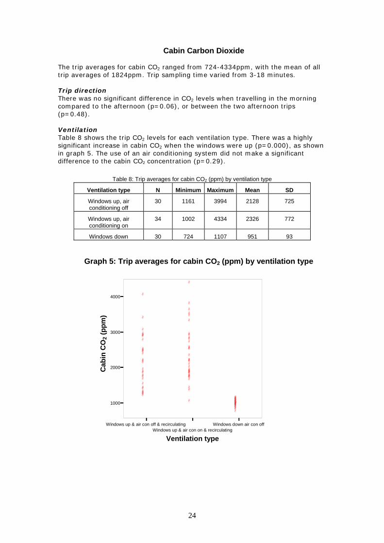
Cabin Carbon Dioxide The trip averages for cabin CO2 ranged from 724-4334ppm, with the mean of all trip averages of 1824ppm. Trip sampling time varied from 3-18 minutes. Trip direction There was no significant difference in CO2 levels when travelling in the morning compared to the afternoon (p=0.06), or between the two afternoon trips (p=0.48). Ventilation Table 8 shows the trip CO2 levels for each ventilation type. There was a highly significant increase in cabin CO2 when the windows were up (p=0.000), as shown in graph 5. The use of an air conditioning system did not make a significant difference to the cabin CO2 concentration (p=0.29).

Table 8: Trip averages for cabin CO2 (ppm) by ventilation type

Ventilation type N Minimum Maximum Mean SD

Windows up, air conditioning off

30 1161 3994 2128 725

Windows up, air conditioning on

34 1002 4334 2326 772

Windows down 30 724 1107 951 93

Graph 5: Trip averages for cabin CO2 (ppm) by ventilation type

Windows up & air con off & recirculating Windows up & air con on & recirculating

Windows down air con off

Ventilation type

1000

2000

3000

4000

Cab

in C

O2 (

ppm

)

!

!

!

!

!

!

!

!

!

!

!

! !

!

!

!

!

!

!

!!

!

!

!

!!

!

!

!!

!

! ! !

!!!!!

!

! !

!

! !

!

!

! !

!!!!!!

!

!

!

!!!

!

!

!

!!

!

!!!

!

!

!

!

!

!

!

!

!

!!!

!

!

!

!!!!!!!

!

!

24

Variation of exposure during journey The CO2 concentration for each second of every trip through the tunnels has been averaged and graphed against time for each ventilation type (Graph 6). The graphs indicate that the longer a vehicle is in a tunnel, the higher the CO2 concentration. When the windows are up, the exposure to CO2 is increased. 3000.

2000.

1000.

Windows down n=30 Windows up, air conditioning off n=30 Windows up, air conditioning on n=34

Category

Graph 6: Averaged one-second cabin CO2 exposure (ppm) by time in tunnel

0.00 2.00 4.00 6.00 8.00 10.00

Time (minutes)

00

00

00

ppm

25

External Carbon Dioxide The trip averages for external CO2 ranged from 594-1502 ppm, with a mean of all trip averages of 911ppm. Trip direction Table 9 shows the trip averages for external CO2 according to trip direction. External CO2 results are also represented in Graph 7. Trip averages were significantly higher in morning compared with afternoon trips (p=0.002); there were also significantly higher trip average levels of CO2 in the eastbound afternoon trip compared with the westbound trip (p=0.01).

Table 9: Trip averages for external CO2 (ppm) by trip direction

Trip Direction N Minimum Maximum Mean SD

Morning east 32 632 1502 980 140

Afternoon west 31 594 1033 824 109

Afternoon east 31 604 1318 927 187

Graph 7: Trip averages for external CO2 (ppm) by trip direction

morning east afternoon west afternoon east

Trip Direction

600

800

1000

1200

1400

Exte

rnal

CO

2 (pp

m)

! !

!

!

!

!

!

!

!

!

!

!

!

!

!

! !

!

! !

!

!

!

!!

! !

!

!

!

!

! ! !

!

!

!

!

!!

!

!

!

! !

!!

!

!

!

!

!!

!!

!

!

!

!

!

!

!

!

!

!

!

!!

!

!

!

!

!

!

!

!

!

! !

! !

!

!

!

!

!

!!

! !

!!

!

!

26

Variation of exposure during journey The external CO2 concentration for each second of every trip through the tunnels has been averaged and graphed against time (n=94 trips), (Graph 8). The external CO2 concentration demonstrates a decrease mid-tunnel due to the tunnels’ ventilation design.

Graph 8: Averaged one-second external CO2 concentration (ppm) by time in tunnel

0.00 2.00 4.00 6.00 8.00 10.00

time (minutes)

600.00

700.00

800.00

900.00

1000.00

Aver

age

exte

rnal

CO

2 (pp

m)

27

PM2.5 - Dustrak Monitoring of PM2.5 was performed only in the cabin. The trip averages for cabin PM2.5 level was in the range 10-526 µg/m3, with a mean of all trip averages of 163µg/m3. Sampling varied from 3-18 minutes. Trip direction An analysis by trip direction shows that the mean of trip average PM2.5 level when travelling eastbound in the morning was 175 µg/m3; for westbound trips in the afternoon, 151 µg/m3; and for eastbound trips in the afternoon, 162 µg/m3. These differences were not statistically significant (p=0.63). Ventilation An analysis of PM2.5 concentrations by type of cabin ventilation showed that trip averages were significantly reduced when the cabin windows were closed (p=0.000). The use of an air conditioning system had no significant effect on PM2.5 levels (p= 0.22). The trip averages for cabin PM2.5 levels by ventilation type are shown in Table 10 and Graph 9.

Table 10: Trip averages for cabin PM2.5 (µg/m3) Dustrak by ventilation type



30 15 268 64 52


34 10 113 51 25

Windows down 30 133 526 388 106

Graph 9: Trip averages for cabin PM2.5 (µg/m3) by ventilation type


Windows down

Ventilation type

0.00

100.00

200.00

300.00

400.00

500.00

PM2.

5 (µ

g/m

3 )

! ! !

! ! ! ! ! ! !

!

!

!!

!

!

!!

!

!

!

!!!

!!!!!!!!

!

!

!!!!!!

!

! ! ! ! !

! ! !

!

!

!

!

!

!

!

!

!

!

!

!

! ! ! !

!!

!

!!

!

!

!

!

!!!

!!

!

!

!

! ! !

!

!

!

!

!

!

!

!

!

28

Variation of exposure during journey The PM2.5 concentration for each second of every trip through the tunnels has been averaged and graphed against time for each ventilation type (Graph 10). The graphs indicate that the longer a vehicle is in a tunnel, the more PM2.5 the passengers are exposed to. When the windows are open, exposure is immediate, and at mid-journey, there is an air exchange, causing a decrease in PM2.5 concentration. When the windows are up, the exposure to PM2.5 is greatly reduced, and there is a gradual increase over time. Graph 10: Averaged one-second cabin PM2.5 exposure (µg/m3) by time in tunnel

Windows down Category

Windows up, air conditioning off =30 nWindows up, air conditioning on

600

PM2.

5 (µ

g/m

3 )

400

200

0.00 2.00 8.00 10.00 4.00 6.00

Time

29

PM2.5 - Gravimetric

One cumulative gravimetric PM2.5 measurement was taken per week. These values are given in Table 11. The mean PM2.5 level for the study was 89µg/m3.

Table 11: PM2.5 Gravimetric monitoring results

Week Number of days

Accumulated time Results (µg/m3)

Percent of time spent monitoring

with windows down (%)

Week 1

30/10-5/11

5 7 hrs 5 mins 51.8 21

Week 2

6/11-12/11

5 7 hrs 55 mins 99.6 38

Week 3

13/11-20/11

6 8 hrs 18 mins 62.2 42

Week 4

21/11-27/11

5 7 hrs 38 mins 90.7 39

Week 5

28/11-4/12

5 7 hrs 1 min 135.4 21

Week 6

5/12-12/12

6 9 hrs 96.3 34

As the concentrations were collected under a variety of ventilation types over weekly trips through the tunnels, an analysis by trip direction or ventilation type is not possible. The study average level for PM2.5 for this method can be compared to the study average using Dustrak of 162µg/m3. This indicates that the Dustrak significantly overestimated the actual fine particle levels in the vehicles.

30

Cabin Nitrogen Dioxide The daily readings for cabin NO2 were in the range 29.5-250ppbv, with a mean of 101ppbv. Samplers were exposed for an average of 88 minutes (range 71 – 100). Trip direction As there was only one NO2 measurement per day an analysis by trip direction is not possible. Ventilation An analysis according to ventilation (Table 12 and Graph 11) shows that NO2 levels are significantly reduced when the cabin windows are closed (p=0.000). The use of an air conditioning system had no significant effect on NO2 levels (p= 0.30).

Table 12: Cabin NO2 levels (ppbv) by ventilation type



10 37.7 154 65.9 35.6


12 29.5 114 52.4 23.8

Windows down 10 151.4 250 195 31.8

Graph 11: Cabin NO2 (ppbv) by ventilation type


Windows down

Ventilation type

50.00

100.00

150.00

200.00

250.00

Cab

in N

O2 (

ppbv

)

!!!

!!!

!!!

!!!

! ! !

! ! !

!!!

! ! !

!

! ! ! ! ! !

!!!

! ! ! ! ! ! !!!

!!!!!!

!!!

!!!

! ! !

!!!

!!!

! ! !

!!!

!!!

! ! ! ! ! !

!!!

!!!

!!!!!!

!!!

31

External Nitrogen Dioxide The daily readings for external NO2 were in the range 144-477ppbv, with a mean of 207ppbv. As there was only one NO2 measurement per day, an analysis by trip direction is not possible.

Graph 12: Distribution of external NO2 (ppbv)

200.00

300.00

400.00

Exte

rnal

NO

2 (pp

bv)

!!!

!!!

!!!!!!

!!!!!!

!!!

!!!

!

!!!

!!!

!!!

!!!

!!!

!!!

!!!!!!!!!

!!!

!!!

!!!

!!!

!!!!!!!!!!!!

!!!

!!!

!!!

!!!

!!!

Graph 13: External NO2 versus cabin NO2 (when windows are closed)

Linear Regression:

50.00 100.00 150.00 200.00 250.00

Cabin NO2 (ppbv)

200.00

300.00

400.00

500.00

600.00

Exte

rnal

NO

2 (pp

bv)

!!!

! ! !

! ! ! !!!

! ! ! ! ! ! !!!

!

! ! ! ! ! !

! ! !

! ! ! ! ! !

! ! ! ! ! ! ! ! !

! ! !

!!!

!!!! ! !

! ! !

External NO2 (ppbv) = 93.54 + 2.00 * no2inppbR-Square = 0.67

Graph 13 demonstrates that there is a significant relationship between external and cabin NO2 levels when the windows are closed.

32

NO2 outliers On 7 November we recorded the maximum external NO2 level of 477 ppbv and the maximum cabin NO2 level for ventilation type 1 of 154 ppbv. An examination of data collection, analysis and entry could not account for this outlier. The cabin and external levels for CO, PM2.5 and BTEX were unremarkable for this day. We reviewed the RTA M5 East air monitoring data and EPA ambient air data for this period. All four M5 East stations recorded monthly maxima for 1-hour and 24-hour nitrogen dioxide on 8 November, as well as high levels for carbon monoxide. EPA RPI data suggest bushfire impacts in Sydney East on 8 November. It seems unlikely that external conditions are related to the high in-tunnel nitrogen dioxide levels we recorded on 7 November. Pearson’s correlation test showed there was no relationship between ambient NO2 levels as measured by the EPA and the tunnel NO2 levels monitored during this study (p=0.40).

33

BTEX Concentrations of the BTEX gases (benzene, toluene, ethylbenzene and 3 xylene isomers) were measured inside the vehicle. One measurement for each gas was obtained for each day. The mean, maximum and minimum concentrations for each are given in Tables 13-14. Outliers Maximum concentrations of benzene and toluene were recorded on 28 November. The concentration of xylene was also high for this day, but was not the highest level measured. Concentrations recorded were up to twice that of the next highest concentration. This occurred when the windows were up and the air conditioning was off. Values recorded were much higher than even the highest value obtained when the windows were down. An examination of sampling procedure, data entry and analysis could not account for this outlier. Review of operator practices (sampler sealing, refuelling, etc) also did not account for this reading. The following analysis is conducted with and without this outlier.

Table 13: Concentrations of BTEX gases (ppbv) including outlier

Gas N Minimum Maximum Mean SD

Benzene (ppbv) 32 4.8 59.3 14.3 10.2

Toluene (ppbv) 32 12.9 86.2 26.7 14.4

Ethylbenzene (ppbv) 32 1.8 17.3 4.75 3.00

Xylene (ppbv) 32 8.3 57.5 23.7 12.2

Table 14: Concentrations of BTEX gases (ppbv) excluding outlier

Gas N Minimum Maximum Mean SD

Benzene (ppbv) 31 4.8 27.1 12.8 6.14

Toluene (ppbv) 31 12.9 49.0 24.8 9.65

Ethylbenzene (ppbv) 31 1.8 17.3 4.65 2.97

Xylene (ppbv) 31 8.3 57.5 23.0 11.7

34

Benzene A maximum benzene concentration of 59.3ppbv was recorded on 28 November with ventilation type 1 (windows up, vents closed, air conditioning off). The next highest benzene level for any ventilation type was 27.1ppbv. The next highest benzene level for ventilation type 1 was 12.5 ppbv on 11/12/02. When the outlier is included, the average benzene concentration is not significantly reduced when the cabin windows are closed (p=0.08). However, when the outlier is excluded there is a significant reduction in benzene levels when the cabin windows are closed (p=0.00). The use of an airconditioning system does not significantly affect the cabin benzene concentration (p=0.46), even when the outlier is excluded (p=0.28). Refer tables 15 -16 and graph 14.

Table 15: Cabin benzene concentrations (ppbv) by ventilation type (including outlier)


Windows up & air conditioning off 10 5.1 59.3 14.0 16.1

Windows up & air conditioning on 12 4.8 16.2 10.5 3.48

Windows down 10 4.9 27.1 19.0 6.48

Table 16: Cabin benzene concentrations (ppbv) by ventilation type (excluding outlier)


Windows up, air conditioning off 9 5.1 12.5 9.00 2.27

Windows up, air conditioning on 12 4.8 16.2 10.48 3.48

Windows down 10 4.9 27.1 19.01 6.48

Graph 14: Cabin benzene exposure (ppbv) by ventilation type

Benzene outlier

Windows up, air conditioning offWindows up, air conditioning on

Windows down

Ventilation type

10.00

20.00

30.00

40.00

50.00

60.00

Ben

zene

con

cent

ratio

n (p

pbv)

!!!!!!

!!!!!!!!!

!!! !!!

!!!!

!!!

!!!!!!!!!

!!!!!!

!!!

!!!

!!!!!!

!!!!!!

!!! !!!

!!!!!!

!!!!!!

!!!

!!!

!!!

!!!!!!

35

Toluene A maximum toluene concentration of 86.2ppbv was recorded on 28 November, at the same time as the benzene outlier discussed in the previous section. The next highest toluene concentration for this ventilation type was 21.9ppbv, and for any ventilation type was 49ppbv (windows down). Even when this outlier is included there is a significant reduction in toluene concentration inside the cabin when the windows are closed (p=0.025, compared to p=0.000 when the outlier is excluded). The use of air conditioning does not make a significant difference to toluene concentration (p=0.65 compared to p=0.05 when the outlier is excluded). Refer Tables 17-18 and Graph 15.

Table 17: Cabin toluene concentrations (ppbv) by ventilation type (including outlier)




Windows down 10 21.4 49.0 35.1 9.54

Table 18: Cabin toluene concentrations (ppbv) by ventilation type (excluding outlier)




Windows down 10 21.4 49.0 35.1 9.54

Graph 15: Cabin toluene exposure (ppbv) by ventilation type

toluene outlier


Windows down

Ventilation type

20.00

40.00

60.00

80.00

Tolu

ene

conc

entr

atio

n (p

pbv)

!!!

!!!!!!!!! !!!

!!! !!!

!!!!

!!!

!!!!!!

!!!

!!!

!!!

!!!

!!!

!!!!!!

!!!

!!!

!!! !!!

!!!!!!!!!

!!!

!!!

!!!

!!!

!!!!!!

36

Ethylbenzene The average ethylbenzene concentration measured inside the study vehicle was 4.75 ppbv (range 1.8-17.3ppbv). The maximum ethylbenzene concentration (17.3ppbv) was recorded on 10 December, when the windows were down. The next highest value recorded was 8.90ppbv, and was also when the windows were down. There is a significant reduction in ethylbenzene concentration when the car windows are up (p=0.01). Excluding the outlier does not change this reduction. Turning on the air conditioning system did not make a significant difference to the ethylbenzene concentration (p=0.86). The minimum, maximum and mean concentrations for each ventilation type, with and without the outlier are given in Tables 19-20.

Table 19: Cabin ethylbenzene concentration (ppbv) by ventilation type (including outlier)




Windows down 10 1.90 17.3 6.73 4.25

Table 20: Cabin ethylbenzene concentration (ppbv) by ventilation type (excluding outlier)




Windows down 9 1.90 8.90 5.56 2.19

Graph 16: Cabin ethylbenzene exposure (ppbv) by ventilation type

ethylbenzene outlier


Windows down

Ventilation type

4.00

8.00

12.00

16.00

Ethy

lben

zene

con

cent

ratio

n (p

pbv)

!!!!!!

!!!!!!

!!!

!!! !!!!!!!

!!!

!!!!!!

!!!!!!

!!!

!!!

!!!!!!

!!!!!!

!!!!!! !!! !!!

!!!

!!!

!!!!!!

!!!!!!

!!!

!!!

37

Xylene Three xylene isomers (p-, m- and o-xylene) were measured inside the study vehicle as it traversed the tunnel. A xylene outlier for ventilation type 1 occurred on 6 November, which was a different occasion to the other outliers. Cabin xylene concentration was significantly reduced when the windows were closed (p=0.002). Excluding the outlier did not change this reduction. Turning on the air conditioning system did not make a significant difference to the xylene concentration (p=0.96). Minimum, maximum and mean concentrations for each ventilation state, with and without the outlier, are given in Tables 21-22.

Table 21: Cabin xylene concentrations (ppbv) by ventilation type (including outlier)

Ventilation Type N Minimum Maximum Mean SD



Windows down 10 13.4 57.5 33.0 15.0

Table 22: Cabin xylene concentrations (ppbv) by ventilation type (excluding outlier)

Ventilation Type N Minimum Maximum Mean SD



Windows down 10 13.4 57.5 33.03 15.0

Graph 17: Cabin xylene exposure (ppbv) by ventilation type

xylene outlier

Windows up, air conditioning of fWindows up, air conditioning on

Windows down

Ventilation type

10.00

20.00

30.00

40.00

50.00

xyle

ne c

once

ntra

tion

(ppb

v)

!!!!!!

!!!!!! !!!!!! !!!!!!!!!!!!!!!!!!!!!!!!!

!!!!!! !!!

!!!!!! !!!!!! !!! !!!!!!!!!!!!

!!!

!!!

!!!!!!

!!!

38

Trends in pollutants

How did the different pollutants correlate?

There was no association between cabin NO2 and cabin PM2.5, or between cabin NO2 and cabin CO, however the different collection methodologies employed do make an association unlikely. The trip CO and PM2.5 for ventilation type 2 did demonstrate an association (graph 18).

m3)

(u

g/

PM

Graph 18: Cabin PM2.5 Dustrak and CO Windows up, air conditioning on and recirculating

0.0 10.0 20.0 30.0

In-Cabin CO (ppm)

0.00

100.00

200.00

300.00

400.00

500.00

2.5

! !

!

! ! !!!

! ! ! ! ! ! !

! ! ! ! ! !

! ! !

! ! ! ! ! !!

!!

pm2.5 average (ug/m3) = 26.77 + 5.09 * incoaveR-Square = 0.31

Number of cars

An analysis of pollutants by number of cars in the tunnel did not show any relationship. This analysis was limited due to the way data on number of cars was collected. The pollutants analysed were measured over a short time period, ie trip durations ranged from 3-18 minutes. Data on number of cars provided by the RTA are for one-hour periods corresponding to the times when the study was being conducted. When concentrations of pollutants were split according to two ventilation types (windows up or windows down), a relationship with number of cars could be seen for PM2.5 when the windows were down, but not for any other pollutant measured (Graphs 19 & 20).

39

windows up windows down

Graphs 19-20: Cabin PM2.5 exposure versus number of cars

Split by windows up or down

Linear Regression:

2000 2500 3000 3500 4000 Total number of cars traveling in both lanes

0.00

100.00

200.00

300.00

400.00

500.00

PM2.

5 av

erag

e (µ

g/m

3 )

!

!

!

!! !

!

! ! !

!

!

! ! !

! ! ! !

!! !!

! ! ! ! ! !

! !

!

! ! ! ! ! !

!!

! !

! !

! ! !

!

! !

! ! !

! ! ! ! ! !

! !

!

!!

2000 2500 3000 3500 4000 Total number of cars traveling in both lanes

! !

!

!

!

!

!

!

! !

!

! !

!!

! !

! !

!

!

!

!

!

!

!

!

!

!

!

PM2.5 (µg/m3) = 101.76 + 0.09 * totlcarsR-Square = 0.29

Cabin and external comparisons

External and cabin measurements were taken for carbon monoxide, carbon dioxide and nitrogen dioxide. It is clear that when the windows are down, the cabin concentrations closely match the external measurements i.e. what is outside is the same as what is inside. Table 23 and Graphs 21-23 illustrate this.

Table 23: Ratio of external pollutant levels to cabin pollutant levels by ventilation type

Ventilation type CO NO2 CO2


0.23 0.30 2.30


0.25 0.25 2.51

Windows down 0.98 0.96 1.07

40

windows down

Cabin CO (ppm)External CO (ppm)

Category

Graph 21: Cabin (windows down) and external CO concentrations (ppm)

Dot/Lines show Means

06.11.02 18.11.02 30.11.02 11.12.02

Date of Monitoring

17.5

20.0

22.5

25.0

27.5 pp

m

Cabin CO2 (ppm)External CO2 (ppm)

Category

Graph 22: Cabin (windows down) and external CO2 concentrations (ppm)

06.11.02 18.11.02 30.11.02 11.12.02

Date of Monitoring

850

900

950

1000

1050

ppm

Cabin NO2 (ppbv) External NO2 (ppbv)

Category

Graph 23: Cabin (windows down) and external NO2 concentrations (ppbv)

06.11.02 18.11.02 30.11.02 11.12.02

Date of Monitoring

160.00

200.00

240.00

280.00

ppbv

41

The Sydney Bushfires December 2002 Major bushfires occurred in the Sydney area over 4-8 December 2002. EPA pollution indices were high, and PM10 readings, as recorded at M5 East freeway air quality monitoring stations, were above the 24-hour air quality standard. The study was monitoring air quality inside the M5 tunnel during this period. Mean PM2.5, CO and NO2 levels for the 4-6 December (excluding the weekend of 7-8 December) are given in Table 24. These values were not significantly different to those measured during the whole study period.

Table 24: PM2.5, CO and NO2 concentrations during the Sydney bushfires compared to the whole study period

Mean/Range during bushfires

Mean/range for whole period

PM2.5 (Dustrak) (ug/m3) 141 (19-524) 163 (10-526)

NO2 external (ppbv) 160 (144-188) 207 (144-476)

NO2 cabin (ppbv) 89.4 (42-169) 101 (29.5-250)

CO external (ppm) 17.4 (7-28) 20.6 (5-39)

CO cabin (ppm) 8.4 (0.1-16.7) 10.4 (0.1-35)

42

5. DISCUSSION AND FINDINGS General This is the first publication in Australia of concentrations of a range of pollutants from the cabin and exterior of a vehicle traversing a road tunnel. For all pollutants measured there were highly significant differences in exposure levels between an open cabin and a closed cabin. The use of a single vehicle for many journeys means that the variability found should derive mainly from variations in tunnel pollutant levels rather than vehicle factors, apart from that tested – ventilation. However the generalisability of these findings to other vehicles is unknown. It is likely that the closed cabin scenario approximates a best-case scenario, as the vehicle was relatively new and well maintained. The windows down scenario may approximate a worst-case, such as may be experienced by motorcyclists or in older vehicles. The long exposure period required for passive sampling (nitrogen dioxide and air toxics) means that the monitoring period does not reflect the typical commuter exposure in the tunnel. The lower sensitivity of passive sampling devices meant that each was exposed for 8 –16 trips per day, an unlikely number of trips for any individual. The need to expose the passive samplers in the non-peak tunnel (morning, westbound) will tend to underestimate the exposure in the peak directions, however this impact is lessened by the ventilation characteristics of the tunnel – air in the first half of the westbound tunnel is derived mainly from the eastbound tunnel, and fresh air exchange occurs at the mid-point. While the sampling methodologies we employed are not specified by current Australian standards, most of these measures have been extensively validated against standard methodologies [15-17]. The Dustrak is acknowledged as having less external validity, depending on the source of particles it is sampling [18], however, we were able to correct this error by using a recognised collection method simultaneously. The carbon monoxide measurements are also validated by strong correlations between levels recorded by the RTA at fixed monitors inside the tunnels and our external levels during afternoon trips. Further validation of these instruments is demonstrated by identical or similar concentrations measured internally and externally when the windows were open. The different methodology for nitrogen dioxide – a passive diffusion sampler – yielded a similar correlation for this ventilation scenario. While it was not a primary focus of this investigation, there appears to be little relationship between tunnel pollutant levels and ambient air. This is not unexpected, due to the concentration of pollutant sources in the tunnel, but would require further investigation to completely explore any relationship. In the two ventilation scenarios with closed windows and vents there was no effect of the use of the air-conditioning system on pollutant levels. Thus these two scenarios can be considered together. Carbon Monoxide We showed that when the vehicle windows are open, carbon monoxide levels increase rapidly from a low background level and parallel the tunnel carbon monoxide levels. As the main tunnel air intake is around the mid-point, CO levels drop here, then rise rapidly again. When the vehicle cabin is closed, carbon monoxide accumulates gradually during the transit, and the impact of the mid-trip fresh air cannot be discerned. This confirms observations from previous studies that air exchange into a closed cabin is relatively slow. At 10 minutes

43

closed cabin levels were on average 6.5ppm, compared to average tunnel levels around 20ppm. This equates to around 2 air changes per hour for this moving vehicle. Work done by the California Air Resources Board in 1997, found that air changes were around 2 per hour for a stationary Ford Explorer with windows closed and vents on recirculate, and rose to around 13 per hour when the vehicle was moving at freeway speeds [19].

Closed cabin CO levels were on average 25% of open cabin levels. The maximum trip exposure for the open cabin of 35ppm did not exceed the 15-minute WHO guideline of 87ppm. The WHO guidelines are set to be protective of the most susceptible individuals – those with ischaemic heart disease and foetuses - from the effects of carbon monoxide. The guidelines are also protective against the acute neurological effects of carbon monoxide such as impaired driving ability. As the longest trip was 18-minutes, comparison to the 30-minute WHO guideline is not warranted; however, trip values were also all below this level. Instantaneous peak values (78ppm) did not approach established limits, such as the Worksafe Australia Short-Term Exposure Limit of 400ppm. Given these findings, tunnel carbon monoxide levels do not pose a risk to public health. Significant differences were observed between morning and afternoon for the cabin and external CO measures. While not reflected in the correlation tests performed, this is probably related to vehicle numbers in the tunnel, which are high in both directions in the afternoon. The lack of correlation between closed cabin CO levels and fixed tunnel monitors demonstrates that individual fixed monitors provide a poor estimate of a motorist’s exposure to CO while in a tunnel if the car cabin is closed. Carbon Dioxide We measured carbon dioxide simultaneously with carbon monoxide to determine if the closed cabin scenario was likely to result in levels that are uncomfortable for occupants. Occupant perceptions of air quality suggest that carbon dioxide concentrations above 1000ppm indicate an inadequate supply of fresh air in mechanically ventilated buildings[20]. Outdoor levels generally range between 400 – 500ppm. We found that the mean trip CO2 with the windows down was 950ppm, however the levels were substantially increased when the windows were wound up. Occupants may thus perceive the cabin conditions as “stuffy” with the windows up and air intake off. The mean levels of CO2 measured external to the vehicle in the tunnel were similar to the levels measured in the cabin with windows down. No carbon dioxide levels reached the level thought to be associated with health effects, around 5000ppm. Observational studies have shown an effect on blood acid balance after several weeks’ exposure at this level, but no effects were observed after 6 hours [21]. It is important to note that CO2 levels are dependent on the number of occupants in the vehicle when window are closed. For vehicles with only one occupant, closed cabin trip levels should be halved, approximately 1100ppm. Of course, if the number of occupants is greater than two, levels will be correspondingly higher. Fine Particles PM2.5 was measured with similar methods to CO and CO2 as well as with gravimetric collection by MicroVol. The pattern of findings with active sampling was similar to CO, however trip averages for fine particles in the closed cabin scenario were only about 15% of the open cabin level. While the Dustrak is a useful methodology, and enables the demonstration of changes in fine particle levels over time as well as relative concentrations, problems with its calibration relative to standard particle methodologies are well recognised [18]. The fine

44

particle levels recorded with the MicroVol are more appropriately compared to health-based dose-response effects. Our MicroVol measurement of PM2.5 used gravimetric collection over all trips during a week. It thus reflects an average level of exposure for all ventilation scenarios. Comparing the two particle collection methods it would appear that the Dustrak overestimated PM2.5 by around 80%. By comparison, a recent Sydney commuter study where exposures were measured for 5 hours in a car found a cabin PM2.5 of 25µg/m3 using a Microvol [23]. We found levels nearly four times this averaged across all ventilation scenarios. Ambient PM2.5 levels during the study period were 17µg/m3 or about 20% of the measured levels in the vehicle. While some investigators have suggested that adverse health effects of fine particles may occur in response to short-term (less than an hour) exposures [24], fine particle standards are based on well-established 24-hour exposure dose-response effects. Individuals with pre-existing heart or lung disease are most susceptible to the effects of fine particles, and effects of increased levels have also been demonstrated on asthmatic children [10], [25], [26]. As there are no health guidelines for fine particle exposure for less than 24-hours, it cannot be predicted whether exposures to these high levels over a usual trip length of 6-minutes, or even during a traffic stoppage, would have an adverse effect on motorists’ health. We provide calculations as to the impact commuting may have on fine particle exposures in Appendix D, which demonstrate that the impact of using the tunnels is small on daily particle exposure. Svartengren exposed asthmatic volunteers to tunnel air in Stockholm for 30-minutes and subsequently assessed lung function for 18 hours. PM2.5 levels averaged 95µg/m3 (range 60-262) in a car with windows closed and fan on measured with a Tapered Element Oscillating Microbalance (TEOM). The measures from a TEOM are comparable to gravimetric collection, and this level is similar to our MicroVol levels, which were collected across the range of ventilation scenarios. Adverse respiratory effects to PM2.5 exposure appeared mild compared to nitrogen dioxide. Subjects with exposure in excess of 100 µg/m3 had a slightly greater early reaction to allergen challenge [27]. Nitrogen dioxide Nitrogen dioxide concentrations were measured simultaneously in cabin and externally with passive samplers. The two measures were very similar on days when the windows in the car were down. While cabin levels were much lower than external levels when the cabin was closed, there was still a strong relationship between external and cabin levels. Air NEPM standards have been developed for application to ambient air, thus the situation we are measuring is not an appropriate application of these standards. The nitrogen dioxide standard is however derived from observations that adverse effects are observed in asthmatics exposed to concentrations above 200 – 300ppbv over 30 to 60minutes [4]. Our collection period is comparable to this trial exposure. It is unlikely that our measures represent any individual’s exposure, as at least four consecutive typical transits of the tunnel are required to accumulate this exposure. However, as tunnel transits can take up to 30minutes, equivalent to the minimum exposure period where the effect on asthmatics is established, there is some justification for comparing worst-case tunnel nitrogen dioxide exposures with this adverse effect level. However, we are also aware that longer transits are associated with incidents such as accidents and breakdowns, in which case the tunnel ventilation is switched to incident mode, emitting air via the portals to rapidly reduce pollutant levels. Our measures do not allow us to identify whether or not incident mode ventilation effectively reduced NO2

exposure.

45

The mean nitrogen dioxide exposure for the open cabin scenario was 195ppbv, and on two occasions the exposure was at or above 200ppbv. Most results from the external measurements also exceeded this level. By contrast, the maximum level experienced with the cabin closed was 154ppbv. Typically ambient NO2 levels in Sydney are well below the standard, and it is uncommon for the Air NEPM standard to be exceeded [5]. In the recent Sydney commuter study, average cabin NO2 levels were below even the minimum cabin level in the tunnels (in type 2 ventilation category) of 29.5ppbv[23]. Thus NO2

exposures in the tunnels represent a significant increase above usual cabin levels, particularly if the windows are open. The usual exposure period for tunnel users is however relatively short. NO2 has rarely been reported from vehicles or tunnels. In Svartengren’s study of asthmatics in a Stockholm tunnel, NO2 levels averaged 141ppbv, compared to the average in this study of 101ppbv. Svartengren determined that subjects exposed to tunnel NO2 levels above 146ppbv for 30 minutes had a significantly greater early reaction following allergen exposure as well as reduced lung function and more asthmatic symptoms compared to those with lower exposure [27]. In our study the concentrations measured with open windows all exceeded 146ppbv. Only on one day in the closed cabin scenario was this level exceeded. There is little information available to determine the minimum length of exposure to NO2 that may precipitate an effect in asthmatics. A Swedish investigator, Barck [described in 28], exposed asthmatics to 240ppbv NO2 for 15minutes and found an increased inflammatory response after allergen challenge. Thus it appears high levels of NO2 can impact on asthmatics following exposures shorter than the 30 minutes previously established. This has obvious implications for situations such as road tunnels. Based on these recent findings of the effect of NO2 on asthmatics, road authorities in Europe are considering setting guidelines for NO2 in road tunnels [28]. We recommend that agencies in NSW should develop a better understanding of NO2

levels in our road tunnels, and work towards developing guidelines to control NO2

exposure, as has occurred for CO. Pending these investigations, motorists can minimise NO2 exposure by closing windows and switching ventilation to recirculate. At present, we also advise road users in open vehicles, such as motorcyclists, who suffer from asthma, to avoid using the tunnels when transit times are likely to be prolonged. BTEX Gases Our study also showed a similar pattern for BTEX gases – levels were in general twice as high with the open cabin scenario compared to the closed cabin. Compared to other studies that have measured these gases in vehicles, levels were not particularly high. It is already established that levels in vehicles are significantly higher than ambient levels (in Sydney these are 1-2ppbv), and that factors such as road congestion and car maintenance and age play an important role in determining in-vehicle levels [19, 29]. No previous studies have focussed on levels in vehicles using tunnels, except for Weisel who found that levels increased 1.5–4 times in a tunnel compared to other New York City commutes [29]. Internationally, in-vehicle benzene levels have varied from around 3ppbv to around 20ppbv, the exception being Chan’s study in Taipei, where the average level in cars was 78ppbv [30]. Benzene levels were previously documented in Sydney cars by Duffy in 1996. Samples were collected during 8 commutes along two congested surface routes, and averaged 22ppbv in post-1986 vehicles. Duffy used three ventilation scenarios – all had windows closed, and varied the use of

46

air conditioner and vents. There was no consistent effect of the scenarios on in-cabin levels, but the study was limited in its ability to detect a difference due to the limited number of samples. The significantly lower levels found in our vehicle for the closed car scenario compared to Duffy may reflect improved vehicle body or exhaust system manufacture. An important factor highlighted by Duffy and other previous researchers is that exposure to BTEX gases is significantly higher in older vehicles. However it is unlikely that any vehicle would experience a higher exposure in the tunnels than our open cabin scenario unless that vehicle were a strong source of BTEX gases due to a malfunctioning exhaust system. In this case, however, occupant exposure would be higher whether or not the vehicle was using a tunnel. Overall, while we have confirmed previous commuter studies demonstrating that BTEX gas levels in vehicles are significantly higher than ambient levels, even the peak levels are several orders of magnitude below those associated with acute health effects. Published acute health lowest effect levels for air toxics include 7.6parts per million for benzene (lowest observed affect level for bone marrow toxicity) [31], 88 parts per million for toluene (neurological effects on workers) [3], around 200parts per million ethylbenzene (eye irritation) [32] and 70 parts per million for xylene (neurological effects) [3]. It is important to note that all these units are parts per million, thus around 1000 times higher than the levels we found in the vehicle cabin. As benzene is a genotoxic carcinogen, it is recommended that exposures should be as low as possible. However, for normal commuters, use of the tunnels even with windows down, does not make a substantial difference to long-term benzene exposure (App D). Unless individuals traversed the tunnels many times per day it is unlikely that exposures from the tunnels would contribute significantly to life-time exposure; however, it is important to note that closing the cabin to tunnel air reduces exposures by approximately half. Comparison to other exposures We present a compilation of pollutant levels measured in other microenvironments in Sydney to provide a context for the levels found in the tunnel. These represent varying collection periods, but as far as possible we have tried to present comparable collection periods to those in this study. An important feature to remember is that the exposure duration in the tunnel is usually short compared to the time spent in most of these other microenvironments, which reduces the likelihood of adverse health impacts.

47

Graph 24: Comparison of PM2.5 levels

0

50

100

150

200

250

300

350

weeklycabin

closed open NSWhomes

commutercar

insidehome near

freeway

outsidehome near

freeway

DarlingHarbour

mic

rogr

ams/

cubi

c m

etre

minmeanmax

For this comparison, we have adjusted the Dustrak readings obtained in open and closed cabin modes by 80% to allow comparison with fine particles collected by more standard methods. The results provided for NSW homes were collected over one week as PM10 and the levels demonstrated here have been adjusted assuming a PM10 to PM2.5 ratio of 0.7 [33]. These indoor levels were collected during winter, with a focus on areas with high prevalence of wood heaters, and included homes where smoking occurred. Those from inside and outside homes near a freeway were collected over 24hours in non-smoking residences in the autumn [34]. Results for commuter cars were collected over 5 hours in spring [23]. The Darling Harbour levels are derived from 10-minute data undertaken outdoors for the Cross City Tunnel project to reflect a peak urban site [35]. This comparison demonstrates that while similar peak levels are found in other microenvironments for PM2.5, the mean level in the tunnels with the windows down is significantly higher than all other microenvironments that have been assessed in Sydney.

Graph 25: Comparison of nitrogen dioxide levels

0

50

100

150

200

250

300

closed open NSW homes commuter car Darling Harbour

ppbv min

meanmax

This comparison of exposure to nitrogen dioxide in microenvironments is sourced from the studies detailed above. The NSW homes levels were averaged over a week, in a range of homes including those using unflued gas appliances, which are strong sources of nitrogen dioxide. Calculated 1-hour levels during unflued appliance use were much higher (20 – 291ppb, median 112ppb) [36].

48

Similarly to the PM2.5 comparison, while peak levels in other settings may be similar in some cases to those found in the tunnels, the tunnel range with open windows demonstrates a significantly elevated mean. The length of exposure in the tunnel is conversely typically much shorter than the other microenvironments, so that the increased level may not translate to an increased risk of health effects.

Graph 26: Comparison of carbon monoxide levels

0

5

10

15

20

25

30

35

40

closed open Darling Harbour 10-min

Darling Harbour 1-hour

Rozelle

ppm min

meanmax

We are aware of less local monitoring in microenvironments for CO than for fine particles and nitrogen dioxide. The comparisons provided here are from the Cross City Tunnel Representations Report, representing a peak urban site in Darling Harbour, and the ambient EPA monitor at Rozelle. A mean value for the 10-minute Darling Harbour data was not published, which limits our ability to make a comparison between the tunnel and peak urban exposure. Again, while the peak values in Darling Harbour are similar to those found in the tunnels, the mean tunnel level appears to be considerably higher.

Graph 27: Comparison of benzene levels

0

5

10

15

20

25

30

closed open BTEX study Perth hot spots Sydney CBD

ppbv

min

mean

max

Additional data sources used in the comparison of benzene include the data in the Environment Australia Technical Report No. 6 – BTEX Personal Exposure Monitoring in Four Australian Cities [32]. The BTEX study results are those from 24-hour sampling of non-smoking volunteers in Sydney, Melbourne, Perth and

49

Adelaide. Part of this report focussed on 12-hour sampling of probable hot spots in Perth. The peak 12-hour level for benzene was in a basement car park. Due to the low concentration of benzene in petrol in Western Australia, it could be expected that levels in a Sydney car park are higher, by a factor of up to three. The Sydney CBD values are the reported 24-hour range from the EA publication. Similarly to most of the other pollutant comparisons made here, the tunnel values only differ substantially from other microenvironments in the mean of the open cabin scenario. While this does seem to represent a significant increase in exposure, the impact of this on health is likely to be small, as all exposures are well below known acute effect levels, and the impact from the short time spent in the tunnel on life-time exposure is very small (App D). Conclusions During the six weeks of peak hour commutes when we sampled in the tunnels we did not find pollutant exposures that exceeded established guidelines. Pollutant levels when the windows were open were significantly higher than when the cabin was closed. Even closed cabin pollutant levels were higher than those found in most other settings. Due to the short transit time this increased level of pollutants known to be associated with chronic effects is unlikely to have a significant impact on health, however closing the vehicle cabin is a simple precautionary measure, and consistent with WHO advice on reduction of life-time exposure to carcinogens. We have identified that road tunnel ventilation systems may need to manage NO2

in a similar way as is currently done for CO, and recommend that NSW agencies collaborate on improving our understanding of tunnel NO2 levels and determining whether short-term exposure guidelines need to be developed. As at times tunnel transits can be prolonged, and pollutant levels may be higher than during our sampling, we believe that a precautionary approach is for commuters to close the vehicle cabin while in road tunnels so that any potential acute impact of elevated pollutant exposure can be minimised. Pending a better understanding of NO2 levels in tunnels we would advise that motorists in open vehicles and motor cyclists avoid using the tunnels when transits are likely to be prolonged, particularly if they suffer from asthma.

50

6. ACKNOWLEDGMENTS The authors gratefully acknowledge many people who made this study possible. We wish to offer huge thanks to all persons in the South Eastern Sydney Public Health Unit who greatly assisted with the project and those persons include Steven Hatzi, Diane Smith, Lauren Booth, Angela Wong and Professor Bernard Stewart. We also seek to gratefully acknowledge the dedication of Rob Gillett, Principal Project Scientist and Jennifer Powell, (Experimental Scientist), of the CSIRO Division of Atmospheric Research who provided air monitoring advice, analysis of samples and ongoing support. Steve Faulkner (M5 East Freeway Development Manager, RTA Motorway Services Branch) who regularly provided traffic statistics. Michael Chertok (Acting Senior Policy Analyst, Air Quality & Physical Hazards, Environmental Health Branch, NSW Health) who provided details of current and past research into this area.

51

7. GLOSSARY Active sampling - Pollutants samples are collected by drawing air into the collector such as a filter or chemical solution for a known period of time. BTEX gases - benzene, toluene, ethylbenzene and xylene Cabin Monitoring – air sampling within the vehicle CSIRO – Commonwealth Scientific and Industrial Research Organisation EPA – NSW Environment Protection Authority Exposure – The dose of pollutant which a person could receive during time spent in a given environment External Monitoring – air sampling outside the vehicle Gravimetric – denoting a method of analysing compound bodies by finding the weight of their elements IARC – International Agency for Research on Cancer µg/m3 - micrograms per cubic metre – a measure of concentration Mean – The sum of all the measurements in a data set divided by the number of measurements in the data set NEPC – National Environment Protection Council, Australia Passive sampling - A sample integrated over a defined exposure time (typically a week to a month) is collected by molecular diffusion to a pollutant-specific absorbent material. Pearson Correlation Co-efficient –A measure of linear association between two variables. Values of the correlation coefficient range from -1 to 1. The sign of the coefficient indicates the direction of the relationship, and its absolute value indicates the strength, with larger absolute values indicating stronger relationships. ppbv – parts per billion – a measure of concentration ppm – parts per million – a measure of concentration Standard Deviation (SD) –A measure of dispersion around the mean. In a normal distribution, 68% of cases fall within one SD of the mean and 95% of cases fall within 2 SD. RTA – New South Wales Roads and Traffic Authority US EPA – United States Environment Protection Agency WHO – World Health Organization

52

APPENDIX A: SUMMARY OF AIR QUALITY STANDARDS

Pollutant Standard Time Average Country Institution

120ppbv 1 hr Australia NEPC [4]

98ppbv 1 hr International WHO [3]

250ppbv 1 hr US (California) SCAQMD [37]

NO2

150 ppb 1 hr UK UK [38]

9 ppm 8 hr Australia NEPC [4]

87 ppm

50 ppm

25 ppm

10 ppm

15 min

30 min

1 hr

8 hr

International

guidelines

WHO [3]

35 ppm 1 hr US USEPA [39]

9 ppm

20 ppm

8 hr

1 hr

US (California) SCAQMD [37]

CO

10 ppm 8 hr UK UK [38]

50 µg/m3 24 hr Australia NEPC [4]

150 µg/m3 24 hr US USEPA [39]

50 µg/m3 24 hr US (California) SCAQMD [37]

PM 10

50 µg/m3 24 hr UK UK [38]

25 µg/m3 24 hour Australia NEPC [6]

Advisory reporting standard for non-peak sites

65 µg/m3 24 hr US USEPA [40]

30 µg/m3 24 hr Canada NEPC [6]

PM 2.5

25 µg/m3 24 hr New Zealand proposed interim guideline [6]

10ppm (3.2 mg/m3) 15 min limit US NIOSH STEL--National Institute of Occupational Safety and Health's

short term exposure limit [41]

Benzene

5 ppbv (16.25 µg/m3) long term - annual

UK UK [38]

53

APPENDIX B: DAILY RECORD MONITORING SHEET

Daily Record Sheet

Date: ___________________________

Ventilation Type: Windows up & air con off with external air intake

Windows up & air con on & recirculating

Windows down air con off

Passive Sampling ID Numbers

CABIN

Nitrogen Dioxide _________________________ BTEX ____________________

PM2.5____________________________________________________________

EXTERNAL

Nitrogen Dioxide ___________________________________________________

TRIP DIRECTION: MORNING EAST Research Officers: TC SC SH Other ___________

Criteria Number of trips

Total Duration

CO (in)

PM 2.5

CO (out)

Incidents: ___________________________________________________________________________________________________________________________________________________________________________________________________

54

TRIP DIRECTION: AFTERNOON WEST Research Officers: TC DS SH Other ____

Number of trips

Total Duration

CO (cabin)

PM 2.5

CO (external)

Incidents: ___________________________________________________________________________________________________________________________________________________________________________________________________

TRIP DIRECTION: AFTERNOON EAST Research Officers: TC DS SH Other ___________

Criteria Total Number of trips

Total Duration

CO (cabin)

PM 2.5

CO (external)

BTEX, PM2.5, NO2

Incidents: ___________________________________________________________________________________________________________________________________________________________________________________________________

55

APPENDIX C: CSIRO ANALYTICAL METHODS According to Ferm (1991) the ambient concentration of the gas of interest, Cx, may be calculated from a knowledge of the amount trapped on the sorbant filter located at the end of the sampler tube, X, the mean absolute temperature, T, during sampling, the diffusion coefficient of the gas of interest, Dx, and a number of geometric factors:

+++=

R

LBL

N

N

F

F

R

R

x AL

AL

AL

AL

TDX

C x , (1)

where: LR is the length of the stagnant tube, AR is the cross-sectional area of the tube, LF the thickness of the membrane filter, AF the total area of pores in the membrane (calculated from the exposed area, AR and the filter porosity), LN is the thickness of the stainless steel screen, AN open area of the stainless steel screen, LLBL is the thickness of the laminar boundary layer that exists in contact with the external face of the sampler. Ferm (1991) measured the laminar boundary layer thickness under a range of ambient atmospheric conditions and suggested a mean value of order 1.5 ± 0.6 mm for LLBL. The first three terms in parenthesis represent the resistances due to diffusion along the stagnant sampler tube, diffusion through the membrane, and diffusion through the stainless steel screen. All three are geometrically fixed. The final term represents diffusion through the laminar boundary layer, the thickness of which will vary with atmospheric turbulence. The membrane filters employed on the samplers were 25 mm MFS, PTFE Cat. No. J100A025A, while the paper filters employed as the trapping medium were 24 mm Whatman paper filters, Cat. No. 1440024. Blanks on the paper filters were virtually eliminated by a clean-up procedure in which the filters were washed in high purity (HPLC-grade) water, twice in AR grade methanol, and dried in a stream of high purity nitrogen. The coating solution for the NO2 sampler was 0.44g NaOH plus 3.95g NaI made up to 50 ml with AR grade methanol. In both cases 50 µl of coating solution was added by pipette to a paper filter that was then placed directly into a sampler body under clean laboratory conditions. Samplers were sent to and from the field in sealed plastic bottles as recommended by Ferm (1991). The reaction to trap NO2(g) on the filter can be expressed as follows :

2NO2 + 3I− → 2NO2− + I3

−.

After exposure the sample filters were extracted in 5 ml HPLC-grade water in sealed plastic bags. The NO2 filter extracts were analysed colorimetrically at 540 nm for nitrite, after mixing with a diazotizing reagent (Ferm, 1991). More Detailed Experimental Section Upon receipt of the sealed sampler, the paper filter is removed and sealed in a small clean polythene bag and stored at 4°C for later analysis. It is extracted in 5 cm3 of Milli-Q water. A NaI solution of 0.79 g NaI l-1 of Milli-Q water is made up and used for dilution of standards so that sample and standards have the same NaI concentration :

56

Table 1. Standard nitrite concentrations. 100 µM 100 µl of 0.1 M NaNO2 diluted with

NaI solution to 100 cm3. (=100 cm3)

75 µM 1.5 cm3 of 100 µM std + 0.5 cm3 of NaI solution. (= 2 cm3) 50 µM 1.0 cm3 of 100 µM std + 1.0 cm3 of NaI solution. (= 2 cm3) 20 µM 400 µl of 100 µM std + 1.6 cm3 of NaI solution. (= 2 cm3) 10 µM 200 µl of 100 µM std + 1.8 cm3 of NaI solution. (= 2 cm3)

5 µM 100 µl of 100 µM std + 1.9 cm3 of NaI solution. (= 2 cm3) 2 µM 40 µl of 100 µM std + 1.96 cm3 of NaI solution. (= 2 cm3)

Reagent solution The following three chemicals should be weighed into a 100 cm3 volumetric flask. The chemicals are dissolved by the addition of Milli-Q water to make a solution of 100 cm3. The solution must be freshly made for each analysis period.

0.8 g sulfanilamide 0.02 g N-1-Naphthylethylenediamine dihydrochloride (NEDA) 0.8 ml H3PO4 Measurement A 2 cm3 aliquot of each standard and of each sample are placed into separate 30 cm3 Nalgene plastic bottles to which an equal amount (2 cm3) of the reagent is added. The solution turns pink. The spectrophotometer is adjusted to a wavelength of λ = 540 nm with the visible lamp turned on and in absorption mode. The samples are left for a 15 minute period so they can fully react, then the absorbances of the samples and standards are measured with the spectrophotometer.

Calculation of ambient NO2 concentration A straight line is fitted to the standards using a least squares regression program. The line is then used to calculate the NO2- concentration in the sample solutions. The concentration of NO2(g) can be calculated in nanomoles m-3 in the same way as for the acid gases, using EV = 5 cm3 and the appropriate diffusion coefficient:

NO2 (g) = L × EV × [SO42−]

T × DC Where : L = total air resistance = 41.2 m-1 EV = extraction volume (cm3)

[SO42-] = sulfate concentration (µmoles l-1 )

T = sampling time (seconds) DC = diffusion coefficient (1.54 x 10-5 m2 sec-1 for NO2)

This figure for NO2(g) can then be converted to ppbv using :

p = n × R × T V

Where : n = number of moles (in a m3) R = gas constant = 0.08206 l atm mol-1 K-1 T = temperature during sampling (°K) V = air volume (=1000 l)

57

BTEX Sampling

Principles of passive gas sampling Diffusive monitoring is a technique that uses the physical process of gas diffusion to collect gases of interest on a solid adsorbent. Such a technique has several important advantages. Some of these are that the sampler is very small, light, uses no power and generates no noise. This makes them eminently suitable for use in personal sampling where high frequency sampling is not required. To be effective, diffusive monitors must be capable of maintaining the following conditions during the sampling process:

• ambient concentration of the components of interest at the surface of the monitor

• zero concentration of the components at the surface of the absorbent material

• a linear concentration gradient between the two (see Figure 1 below).

Figure 1. Principles of diffusive sampling

Under these conditions, Fick’s 1st law of Diffusion applies and components will migrate to the adsorbent at a rate, which is dependent on:

• The path-length between the top surface of the monitor and the adsorbent bed

• The cross-sectional area of the sampler • The time of exposure • The diffusion coefficient of the analyte through air

58

• The ambient concentration of the components

This can be expressed by the formula:

(1)60 1

ZADUm

××=

Where: Um = sampling rate (cm3 min-1)

D1 = diffusion coefficient through air of the vapour under study (cm2 s-1).

A = cross-sectional area of the sampling tube (cm2). Z = path-length of the air gap (cm). In this case, for the ATD 400 Perkin-Elmer tube, A = 0.2 cm2 and Z = 1.5 cm.

If the gas mixing ratio is required in ppmv a published uptake rate can be used or else it can be calculated from the following expression:

Up =60 × D1 × A × MWgas

Vm × Z(2)

where : Up = Uptake rate (ng ppm-1.min-1). MWgas = molecular weight of gas of interest (g). Vm = molar volume (L). The mixing ratio (C) of a compound in ppbv can then be calculated from:

C =Wt ×1000

Up × T(3)

where :

Wt is the mass of sample adsorbed on the Chromosorb 106 in the tube (ng)

BTEX sampler design The aim of the sampling procedure is to adsorb BTEX (benzene, toluene, ethyl benzene, o-xylene, m-xylene and p-xylene) gases onto the absorbent bed during the period of exposure. The adsorbent is packed into a stainless steel tube 6.35 mm diameter and 90 mm in length. For this study the BTEX samplers will be packed with Chromosorb 106. Figure 2 shows a diagram of a BTEX sampler fitted with a diffusion cap. The BTEX samplers will be pre-cleaned before each sampling period by heating under a stream of ultra high purity helium and then sealed with Swagelok caps using PTFE ferrules. The cap should be tightened to ensure that the BTEX sampler is sealed to at least 3 psi; this is sufficient to allow for the lower pressure the BTEX samplers will experience during transportation by air. The BTEX samplers will be transported by airfreight, tightly sealed in a metal container. Charcoal bags will be added to absorb any BTEX gases in the unlikely event they penetrate the metal container.

59

Figure 2. Diagram of a BTEX sampler BTEX Analysis Adsorbed BTEX species are desorbed by heating the tubes under a stream of ultra

high purity helium gas in a Perkin Elmer ATD 400 thermal desorber (automated

thermal desorber). The desorbed species are transferred through a heated line to a

Perkin Elmer AutoSystem XL gas chromatograph where they are separated by an SGE

BP 20 column and detected with a flame ionization detector. Table 1 gives details of

the column and temperature program used for the analysis.

Table 1. Gas Chromatography conditions

Item Description Column 25 m x 0.32mn I.D. fused silica capillary

column with 1.0 µm BP20 bonded phase Injector ATD 400 (mode 2) Carrier gas Helium 50psig Oven Temperature 60°C for 6 minutes programmed at

20°C min-1 to 220°C Detector Flame Ionization Detector

A test calibration has been carried out using the Perkin Elmer system. Peak areas were

determined by integration using a Turbochrom workstation and converted to mass

after injection of standards. The standard is a mixture of benzene, toluene, ethyl

benzene, m-xylene and o-xylene with mixing ratios of 10.1 ppm, 10.1 ppm, 10.1 ppm,

10.1 ppm and 10.0 ppm respectively and an accuracy of ± 2% (Scott Specialty Gases,

San Bernadino, CA, USA). Since the chemical properties of p-xylene are similar to

m-xylene the m-xylene calibration was applied to p-xylene.

60

The calibration was carried out by loop injection onto the ATD during each analytical

run. For all calibrations the loop was flushed for 1minute with the BTEX standard at a

flow rate of between 50 and 60 cm3 min-1. The loop volume was 812 µl and it was

heated to 80°C (353K). The mass of each species injected during each calibration is

given in Table 2 and was calculated as follows:

(4)TR

MWCVmass gasgasloop

×××

=

Where : R = gas constant (0.082054 l atm mol-1 K-1) T = temperature (353K) Vloop = loop volume (0.000812 l) MWgas = molecular weight of gas of interest (g). Cgas = gas concentration (ppmv)

Table 2. Mass of gases for one ATD loop injection

Gas Mass injected (ng) Benzene 22.15 Toluene 26.12 Ethyl-benzene 30.12 m-xylene and p-xylene 30.12 o-xylene 29.82

Therefore, dividing this mass by the peak area, gives the mass per unit area ratio

and multiplication of this ratio by the peak area of each species gives the mass of

each species collected by the passive sampler.

The ATD 400 enables the analysis of up to 50 samples and entire procedure can be

automated from desorption of the sample tube to the final printed report. The system

utilizes a unique electrically-cooled, packed cold trap minimizing the risk of

blockages by ice-plug formation and allowing compatibility with samples containing

significant amounts of water.

There are two modes of operation to be used in the pilot trial:

• Mode 1 is tube conditioning which is employed to purge the tubes

before they are used.

61

• Mode 2 is a two stage desorption that allows the tubes to be

analysed; Table 3 shows the ATD 400 settings employed during

the mode 2 desorption stage.

Table 3. ATD 400 Conditions for mode 2.

Procedure Setting Mode 2 Primary desorption 220°C Primary desorption time 1 min Transfer line temperature 200°C Cold trap low temp -30°C Cold trap high temp 200°C Inlet split flow No Primary desorption Time Depends on experiment Transfer line temperature Depends on experiment Valve temperature 175°C Cold trap hold 1 min Trap fast Yes

Analysis of the BTEX samplers was performed at CSIRO Atmospheric Research, Aspendale, Victoria.

62

APPENDIX D: CALCULATIONS OF EXPOSURE INCREMENT FOR NON-THRESHOLD POLLUTANTS PM2.5

Assuming: Ambient concentration: 17µg/m3

Usual commuting cabin concentration: 25µg/m3

Cabin concentration in M5 tunnel: 89µg/m3

Commute duration#: 79mins/day Tunnel duration: 13mins/day Cigarettes/day 0 Exposure to ETS: 0 Home heating: electric Then: Daily PM2.5 exposure = (time *ambient+ time(commuting-tunnel) *commute + timetunnel*tunnel)/24 ambient

= (1361mins*17µg/m3 + 66mins*25µg/m3 + 13mins*89µg/m3)/24 = 18µg/m3

By contrast, for a similar commuter not using the tunnel, daily PM2.5 exposure is estimated to be 17.4µg/m3. Benzene Assuming: Ambient concentration²: 1.4ppbv

Usual commuting cabin concentration: 12.1ppbv

Cabin concentration in M5 tunnel (windows down): 19ppbv

Commute duration: 79mins/day Tunnel duration: 13mins/day Cigarettes/day 0 Exposure to ETS: 0 Home heating: electric Then: Daily benzene exposure = (timeambient*ambient+ time(commuting-tunnel) *commute + timetunnel*tunnel)/24 = (1361mins*1.4ppbv + 66mins*12.1ppbv + 13mins*19ppbv)/24

63

= 2.05ppbv

The exposure for a similar commuter not using the tunnel, is not substantially different at 1.98ppbv. Following the methodology of Wadge and Salisbury (National Environmental Health Forum Monograph, Benzene, 1997), the impact on lifetime benzene exposure can be calculated as follows: Assuming a respiration rate of 0.83m3/hour, and a conversion of 1ppbv benzene to 3.24µg/m3, and using a scenario of living in a suburb and commuting daily by car to Sydney CBD for 79 minutes round trip: Intake during commuting: Using tunnel: (13min*61.6µg/m3 + 66min*39.2µg/m3 ) * 79min * 0.83 m3/60min= 46.9µg Alternate commute (39.2µg/m3 *79min)*79min*0.83 m3/60min = 42.8µg Intake from 8.5hr to 9.7µg/m3 (3ppbv) ambient city benzene: (9.7µg/m3 *8.5hr) * 0.83m3/hour = 68.6µg Intake from 14.2hr to 1.3µg/m3 (0.4ppbv) ambient suburban benzene: (1.3µg/m3 * 14.2) * 0.83m3/hour = 15.3µg On a lifetime basis, assuming a working life of 40years, with commuting 5 days/week and 48 weeks/year: Intake during commuting using tunnel: 5 days/week * 48 weeks/year * 40years * 46.9µg = 450 240µg benzene Intake during commuting alt route: 5 days/week * 48 weeks/year * 40years * 42.8µg = 410 880µg benzene Intake over 40years, excluding commuting: (5 days/week * 48 weeks/year * 40years * 68.6µg) + (5 days/week * 48 weeks/year * 40years * 15.3µg) + (124days/year * 1.3µg/m3 * 24hours * 0.83m3/hour) = 808 651µg benzene Total working life benzene exposure (including tunnel): =1 258 891µg benzene Thus commuting contributes approximately 36% of benzene exposure. The working life benzene exposure can be reduced by about 3% by avoiding the tunnel, or closing the vehicle windows. By contrast, Wadge and Salisbury estimated that additional intake of benzene for a 20 cigarette/day smoker would be 8 760 000µg (approx 700% increase). ²from NSW EPA “Ambient Air Quality Research Project (1996 – 2001) Dioxins, Organics, Polycyclic Aromatic Hydrocarbons and Heavy Metals” sourced at http://www.epa.nsw.gov.au/publications/dioxinsorganicsetc.pdf , June 2003. Assuming a commuter spends 9 hours a day at CBD levels (3ppbv) and the remainder of the day at suburban levels (0.4ppbv) # from NSW Transport Data Centre – typical commute duration in Sydney.

64

http://www.epa.nsw.gov.au/publications/dioxinsorganicsetc.pdf

REFERENCES 1. Sinclair Knight Merz, M5 East Sub-regional Air Quality Management Plan.

2002, RTA: Sydney.

2. Sinclair Knight Merz, M5 Motorway East Before and After Opening Traffic Study. 2003: St Leonards.

3. World Health Organisation, Air quality guidelines. 1999, WHO, Geneva.

4. National Environment Protection Council, National Environment Protection Measure for Ambient Air Quality. 1998, NEPC: Adelaide. p. 15.

5. Environment Protection Authority NSW, NSW State of the Environment 2000 (SoE 2000). 2000, EPA, NSW, Sydney.

6. National Environment Protection Council, Discussion Paper: Setting a PM2.5 Standard in Australia. 2002, NEPC: Adelaide. p. 55.

7. Roychowdhury A. and Kumar P. Killer Particles: Deadly Particles. Down to Earth 8(14). 1999.

8. Wilson R. and Spengler J. Particles in Our Air, Concentrations and Health Effects. 1996: Harvard University Press, Harvard, USA.

9. Petroeschevsky A. Simpson RW. Thalib L. and Rutherford S. Associations between outdoor air pollution and hospital admissions in Brisbane, Australia. Archives of Environmental Health, 2001. 56(1): p. 16.

10. Morgan G. Corbett S. Wlodarczyk J. Lweis P. Air pollution and daily mortality in Sydney, Australia, 1989 through 1993. American Journal of Public Health, 1998. 88(5): p. 759-64.

11. Simpson RW. et al. Associations between outdoor air pollution and daily mortality in Brisbane, Australia. Archives of Environmental Health, 1997. 52(6): p. 442-54.

12. Simpson R. et al. Effects of ambient particle pollution on daily mortality in Melbourne, 1991-1996. Journal of Exposure Analysis and Environmental Epidemiology, 2000. 10(5): p. 488-96.

13. Environment Protection Authority Vic, Ambient air pollution and daily hospital admissions in Melbourne 1994-1997. 2001, EPA Victoria: Melbourne. p. 84.

14. US Environmental Protection Agency, Air Toxics Website Benzene Hazard Assessment. 2002, USEPA.

15. Ayers GP. et al. Validation Of Passive Diffusion Samplers For So2 And No2 Under Australian Conditions. Atmospheric Environment, 1998. 32: p. 3587-3592.

16. http://www.tsi.com/iaq/products/qtrak/qtrak_support.htm#specifications, Accessed on July 1, 2003.

17. International Standards Organisation DIS16017-2, September 1998.

18. Sourced at http://www.tsi.com/exposure/products/dusttrak/dusttrak.htm, Accessed on July 1, 2003.

19. Rodes CS. et al. Measuring Concentrations of Selected Air pollutants Inside California Vehicles. 1998, Californial Air Resources Board.

65

20. Western Australian Taskforce on Passive Smoking in Public Places, Task force on passive smoking. 1997, University of WA Department of Public Health: Perth. p. Appendices.

21. Tomes Plus Hazard Text. Sourced at http://csi.micromedex.com, Accessed July 1, 2003.

23. Chertok M. Voukelatos A. Sheppeard V. Rissel C. Comparison of commuter pollutant exposures by transport mode. In preparation.

24. Peters A. Dockery DW. Muller JE. Mittleman MA. Increased particulate air pollution and the triggering of myocardial infarction. Circulation, 2001. 103(23): p. 2810-2815.

25. Lewis PR. et al. Outdoor air pollution and children's respiratory symptoms in the steel cities of New South Wales. Medical Journal of Australia, 1998. 169: p. 459-463.

26. Goldberg MS. et al. Identifying subgroups of the general population that may be susceptible to short-term increases in particulate air pollution: a time-series study in Montreal, Quebec. Research Report (Health Effects Institute), 2000(97): p. 7-113; discussion 115-20.

27. Svartengren M. et al. Short-term exposure to air pollution in a road tunnel enhances the asthmatic response to allergen. The European Respiratory Journal : Official Journal of the European Society For Clinical Respiratory Physiology, 2000. 15(4): p. 716-24.

28. Swedish National Road Administration, Air Quality in Road Tunnels: Health Effects of Nitrogen Dioxide and Aspects on Co-pollutants. 2003: Sweden.

29. Duffy BL. Nelson PF. Exposure to emissions of Benzene, 1,3-butadiene and CO in the cabins of moving motor vehicles. 1996, CSIRO: Sydney. p. 41.

30. Batterman SA. Peng C-Y. Braun J. Levels and composition of volitile organic compounds on commuting routes in Detroit, Michigan. Atmospheric Environment, 2002. 36: p. 6015-6030.

31. National Industrial Chemicals Notification and Assessment Scheme, NICNAS Priority Existing Chemical Assessment Report No21. 2001, National Industrial Chemicals Notification and Assessment Scheme: Sydney.

32. Environment Australia, Technical Report No6 BTEX Personal Exposure Monitoring in Four Australian Cities. 2003: Canberra.

33. Sheppeard V, Corbett S. Morgan G. Indoor Air Pollution in New South Wales. The 16th International Clean Air and Environment Conference, Clean Air Society of Australia and New Zealand. 2002. Christchurch.

34. Sheppeard V. Corbett S. Goldthorpe I. Capon A. Fine Particle Levels Near A Busy Motorway. The 16th International Clean Air and Environment Conference, Clean Air Society of Australia and New Zealand. 2002. Christchurch.

35. Roads and Traffic Authority, Cross City Tunnel Representations Report, Appendix 9 Air Quality Monitoring Report. 2001, Holmes Air Sciences: Sydney.

36. Sheppeard V, Unpublished data.

37. South Coast Air Quality Management District, Proposed Draft 2003 Air Quality Management Plan. 2003, South Coast Air Quality Management District: Los Angeles.

38. Department of the Environment, Transport and the Regions in partnership with the Scottish Executive, The National Assembly for Wales and the

66

Department of the Environment in Northern Ireland. The Air Quality Strategy for England, Scotland, Wales and Northern Ireland. 2000: London.

39. The South Coast Air Quality Management District, Smog and Health. 1996, AQMD (California).

40. US Environmental Protection Agency, 1997 Summary Report: Particulate Matter. 1997, USEPA.

41. US Environmental Protection Agency, National Air Toxics Program: The Integrated Urban Strategy Report to Congress. 2001, USEPA.

67

m5 east tunnels air quality monitoring project report july ... · south eastern sydney public...

Documents