m ossbauer spectroscopy - mitweb.mit.edu/8.13/www/jlexperiments/jlexp13.pdf · with the germanium...

Mossbauer Spectroscopy

MIT Department of Physics(Dated: November 29, 2012)

The Mossbauer effect and some of its applications in ultra-high resolution gamma-ray spectroscopyare explored. The Zeeman splittings, quadrupole splittings, and chemical shifts of the 14 keVMossbauer gamma-ray line emitted in the recoilless decay of the first excited state of the 57Fe nucleusare measured in iron and in various iron compounds and alloys. From the data and knowledge of themagnetic moment of the 57Fe ground state one determines the magnetic moment of the first excitedstate. Strength of the magnetic field at the sites of the iron nuclei in metallic iron, Fe2O3, and Fe3O4

are determined. The natural line width of the 14 keV transition is determined from measurementsof the absorption line profiles in sodium ferrocyanide absorbers of various thicknesses. Relativistictime dilation is demonstrated by a measurement of the temperature coefficient of the energy of the14 keV absorption lines in enriched iron.

PREPARATORY PROBLEMS

1. Derive an exact relativistic expression for the re-coil energy of the nucleus of mass M that emits agamma ray of energy E, and evaluate it for an ironnucleus and E = 14.4 keV.

2. Suppose the above atom is embedded in an ironcrystalite which has a mass of 10−6g grams andis free to move. Compute the recoil energy of thecrystal. If the emission of the gamma ray is “recoil-less”, i.e. the nucleus does not acquire momentumrelative to the center of mass of the crystal, whatwould be the energy shift of the gamma ray photondue to the recoil of the crystal?

3. Draw an energy level diagram of the 5726Fe nucleus

in a magnetic field and show the transitions whichgive rise to the Zeeman pattern you expect to seein this experiment.

4. Why is the multiplicity of energy levels of a nu-cleus due to electric quadrupole interaction withan electric field gradient acting alone (quadrupolesplitting) less than the multiplicity of levels due tomagnetic dipole interaction with a magnetic field(Zeeman splitting)?

5. How fast must the source be moved relative to theabsorber to shift the frequency of resonant absorp-tion by the natural line width?

6. Why can’t you do this experiment with the 6.4 keVphotons also emitted by the source?

I. INTRODUCTION

The resolution of a spectrum measurement is charac-terized by the ratio E/∆E, where E is the energy of thespectrum line and ∆E is a measure of the line width ,e.g. the full width at half maximum. The NaI scintilla-tion spectrometer in the Compton experiment producesa spectrum of 662 keV gamma rays with a resolution ofabout 10. At the same energy the spectrum obtained

with the germanium solid state cryogenic detector in theX-ray Physics experiment has a resolution of 200. Thehigh resolution gratings used in the hydrogenic atom ex-periment for measurements in the visible portion of thespectrum has a resolution on the order of 5× 104.

Now imagine spectroscopy with a resolution of1012! “Recoilless” emission and resonance absorptionof gamma radiation by nuclei discovered by RudolfMossbauer in 1957 makes possible such ultra-high reso-lution spectroscopy in the gamma-ray region of the spec-trum. Mossbauer spectroscopy has been used in manyareas of physics and chemistry, for example in the de-termination of life-times of excited nuclear states, in themeasurement of nuclear magnetic moments, in the studyof electric and magnetic fields in atoms and crystals, andin the testing of special relativity and the equivalenceprinciple. The phenomenon itself is also of great inter-est. In this experiment you will observe the Mossbauereffect and explore several of its applications in ultra-highresolution spectroscopy.

Mossbauer himself provided a particularly lucid in-troduction to the physics and application of recoillessgamma-ray emission and absorption in his 1961 NobelLecture which is available in the Junior Lab E-Library[1]. More technical discussions are found in [2, 3]. Anexcellent reference is “The Mossbauer Effect” by HansFrauenfelder [4] which contains historical and theoreti-cal background and reprints of articles bearing on all thetopics in this set of experiments.

You will use as the source of recoilless gamma rays acommercial Mossbauer source consisting of 57

27Co diffusedinto a platinum substrate. The 57

27Co nucleus decays byK-electron capture to an excited state of 57

26Fe accordingto the scheme shown in Figure 1. The newly created ironatom settles down in the crystal lattice of the substrateand the d-shell vacancies in its electronic structure arefilled in such a way as to eliminate the magnetic fieldat the nucleus. 91% of the excited iron nuclei decay bygamma-ray emission to the first excited state (3/2-). Thelatter has a comparatively long half-life of 9.8 × 10−8

seconds (beware that both Melissinos (2003) and Fraun-felder (1962) list the lifetime incorrectly as 0.14 µs) anddecays to the ground state with the emission of 14.4 keV

Id: 13.mossbauer.tex,v 1.107 2012/11/29 15:19:39 abirkel Exp

Id: 13.mossbauer.tex,v 1.107 2012/11/29 15:19:39 abirkel Exp 2

1/2

3/2

5/2 -

-

-

spin-parity

Fe57

7/2 -

electron capture

1/2

9% 0.122 MeV 91%

0 stable ground state of Fe

-7

57

Mossbauer line

Co57

1/2

0.137 Mev ( t =270 days )

0.01437 Mev ( t = 1.4 x 10 s )

FIG. 1. Decay scheme of 5727Co. The 14.4-keV transition 3/2−

− > 1/2 is the one used in many Mossbauer experiments.From http://isotopes.lbl.gov/.

gamma rays of which a substantial fraction are emittedwithout recoil or Doppler broadening. The natural linewidth of the 14.4 keV line is Γ = h ln 2

2πτ1/2= 4.7× 10−9 eV

corresponding to a fractional width of ≈ 3×10−13. In theabsence of a field, the magnetic substates of the excitedand ground states are degenerate. Under this conditionthe spectrum of gamma rays from the recoilless emissionsappears as a single ultra-narrow line on top of a Doppler-broadened and recoil-shifted “normal” emission line, asillustrated in Figure 2a.

In a similar way, absorbers containing 5726Fe can have

ultra-narrow recoilless resonance absorption lines on topof a normal Doppler-broadened and recoil-shifted 14.4keV line. Mossbauer absorption lines may be shiftedslightly in energy with respect to the emission line byvirtue of the different electronic environments of the nu-clei in the source and the absorber (the “chemical” shift),and they may be split by the interactions between thenuclear magnetic dipole and/or electric quadrupole mo-ments with internal or external fields in the absorber(Zeeman or electric quadrupole splittings). In a famousexperiment that tested the red shift predicted by the gen-eral theory of relativity, the shift was caused by a ≈ 100foot difference in height of the source and absorber!

Figure 2b is a schematic representation of the absorp-tion cross section of 57Fe++ in an ionic compound inwhich the iron nuclei are in a nonuniform electric fieldwhich produces an electric quadrupole splitting ∆ε inaddition to an isomer shift δε (see below). The measure-ment process in Mossbauer spectroscopy uses the Dopplershift produced by controlled motion of the source to scanthe emission line back and forth in energy over the ab-sorption spectrum of a sample containing the same iso-tope in its ground state and in a particular chemical orphysical environment of interest. The advantage of usinga source with a single emission line for performing sucha scan is apparent from a consideration of the complica-tions that occur if a multi-line source is used to scan the

FIG. 2. (a) Schematic plots against energy, E, of (top) theintensity, I(E), of gamma rays from a single line Mossbauersource moving with velocity v relative to a Mossbauer ab-sorber, and (bottom) absorption cross section σ(E) of theabsorber. (b) Schematic plot of counting rate C(V) of a de-tector exposed to the gamma rays after they have traversedthe absorber against velocity V. In (a) the energy separationof the two absorption lines is ∆ε , and the Doppler shift dueto the motion of the source is δε . In (b) the velocity separa-tion of the two lines is ∆V = c∆ε

E0, where E0 is approximately

the average energy of the two lines.

absorption spectrum of a multi-line absorber.A primary objective of this experiment is to determine

the width of the convolved recoilless emission and ab-sorption lines of the 14.4 keV transition in 57

26Fe. Thevelocity width Γν corresponding to a given energy widthΓ is given by the simple formula Γν = cΓ/E0 where E0

is the mean energy (14.4 keV) of the gamma rays in theline, and c is the speed of light. The velocity width cor-responding to the natural line width estimated above is1 × 10−4 m s−1. Clearly, one will require a velocity res-olution at least an order of magnitude smaller to obtaina useful profile of the line shape.

Suppose that the recoilless photons are emitted with adistribution in energy, I(E), centered around E0. Whenthe source moves at a velocity V toward the absorber, aphoton emitted with energy E in the rest frame of thesource has an energy

E′ = E

(1 +

V

c

)(1)

in the rest frame of the absorber. (By convention, posi-tive velocity indicates the source moving toward the ab-sorber.) Call σ(E) the cross-section for absorption bythe absorber atoms of photons of energy E, and call ηthe effective area of the detector which we assume to beconstant over the narrow energy range of the 14.4 keVline. Then the counting rate when the emitter is moving


with velocity V will be

C(V ) = η

∫ ∞0

I(E)e−σ(E′)Nx

A dE, (2)

where x is the thickness of the absorber in g cm−2, Ais the atomic weight, and N = 6.022 x 1023 mol−1 isAvogadro’s number. We assume that both the emissionline intensity and the absorption cross section have theLorentzian form, i.e.

I(E) =I0(Γ

2 )2

(E − E0)2 + (Γ2 )2

, and (3)

σ(E) =σ0(Γ

2 )2

(E − E0 −∆E)2 + (Γ2 )2

, (4)

where ∆E is the intrinsic shift of the resonance energyin the absorber relative to the source due to chemical orother effects, and I0 and σ0 are the values at the linecenters. The counting rate of a detector placed in thebeam of gamma rays after the beam has traversed theabsorber is then

C(V ) = ηI0

∫ ∞0

dE(Γ

2 )2

(E − E0)2 + (Γ2 )2

e−

σ0Γ2

2

(E[1+VC

]−E0−∆E)2+( Γ2

)2NxA. (5)

For thin absorbers σ0NxA � 1, and one can obtain an

approximate expression for the line profile by expandingthe exponential factor in Eqn. 5 and keeping only thefirst two terms. The integral can then be evaluated bycontour integration in the complex plane to obtain

C(V ) = C0

(1− B

(E0Vc −∆E)2 + Γ2

), (6)

where C0 is a constant that depends on the strengthof the source and the thickness of the absorber and Bis a constant that depends only on the thickness of thesource. This function has a minimum at V = ∆E

E c and a

full width at half maximum (FWHM) of 2cΓE0

. For thickabsorbers one must resort to numerical integration ofequation (5). Figure 3 shows the line profiles for var-ious thicknesses of absorber corresponding to values ofα = σ0Nx

A ranging from 0.1 to 10. The width of theabsorption line at half amplitude clearly increases withincreasing absorber thickness in the range of thicknesswhere nearly all the recoilless emission is absorbed nearthe line center, i.e. in the range of “line saturation”. Onecan correct for this saturation effect by measuring the linewidth as a function of absorber thickness and extrapolat-ing to zero thickness. (Note that in an actual observationthe non-recoilless emission causes a background countingrate that does not vary with velocity but does decreasewith increasing thickness of the absorber.)

Many interesting effects can be observed in absorptionspectra; several are discussed below.

��

FIG. 3. Calculated shapes of recoilless gamma-ray absorp-tion lines for various thicknesses of absorber. The normalizedcounting rates are plotted as functions of velocity expressedin units of cΓ

E0−∆E≈ cΓ

E0.

II. OBSERVABLE EFFECTS

II.1. Zeeman splitting in an internal magnetic field

The nucleus of an iron atom in metallic iron and certainiron compounds is in an intense magnetic field producedprimarily by unpaired electrons of the same atom. Sinceboth the nuclear states involved in the 14.4 keV transi-tion have spin and associated magnetic moments, bothare split by the interactions between the nuclear mag-netic moment and the magnetic field of the electrons. Inan isolated atom the effect of this interaction on opticaltransitions is characterized as hyperfine splitting. Whenthe atom is bound in a crystal lattice the orientation ofthe internal magnetic field due to the electrons is fixedwith respect to the lattice. As a result, the effect of theelectronic magnetic field on the energy of the nucleus maybe thought of and analyzed simply as the Zeeman effectin a new context. The number of absorption peaks andtheir separations depend on the angular momenta andassociated magnetic moments of the absorber nucleus ineach state. A measurement of the internal Zeeman split-ting can be combined with knowledge of the magneticmoment of the ground state (which can be derived fromother experiments) to deduce the magnetic field at theiron nucleus in the absorber, and the magnetic momentof the first excited state.

II.2. Isomer shift

If the chemical environment of the iron nuclei in thesource and absorber are different then the electron den-sities will, in general, be different. Since the electromag-netic interaction between the electrons and the nucleusdepends, albeit only slightly, on the electron density atthe nucleus and on the nuclear radius, and since the ra-dius of the iron nucleus changes slightly in the 14.4 keVtransition, there is, in general, a shift of the resonance


32

1

34

1

Unpolarized Polarized (theta = 90)

FIG. 4. Expected relative intensities of the Zeeman patternof 57Fe for an unpolarized absorber and for an absorber po-larized perpendicular to the direction of propagation[5].

energy from source to absorber if the host materials aredifferent. This is called the “isomer shift” because the ex-cited states of nuclei were originally called isomers. Themagnitude of the shift depends on the s-electron den-sity at the nucleus. If there is greater electron density atthe absorbing nucleus than at the emitting nucleus, addi-tional energy must be given to the gamma-ray by movingthe source toward the absorber. There are differences onthe order of a factor of ten between the isomeric shiftsof Fe in the +2 and+3 ionization states in the lattice,and these differences may easily be measured. An iso-mer shift in a Zeeman or quadrupole pattern appears asa shift of the “center of gravity” of the lines.

II.3. Electric Quadrupole Splitting

The nucleus may be in an electric field with a gradientdue to nearby ions with unfilled atomic levels. If thenucleus has a quadrupole (or higher) electric moment,i.e. if its electric charge distribution is not sphericallysymmetric, its energy levels will be split by amounts thatdepend on the projections of its spin in the direction ofthe field gradient. The ground state is shifted by thequadrupole interaction, and the first excited level is splitinto two levels: thus two transitions with energies ∆E2±12∆E3, are possible, yielding two absorption peaks, asshown in Figure 2.

II.4. Anisotropic emission by polarized nuclei

Each of the possible transitions that give rise to theZeeman spectrum of lines of an absorber with 57Fe nu-clei in a strong internal magnetic field has a particularanisotropic radiation pattern relative to the direction ofthe field. The orientation of the internal field of a ferro-magnetic material can be controlled by a much weakerexternal field. Thus changes in the relative intensities ofthe lines in the Zeeman pattern can be caused by placingthe absorber in the field of a strong permanent magnet.Figure 4 shows the expected intensities of the Zeemanabsorption lines in an absorber with no preferred orien-tation (unmagnetized) and in an absorber magnetized ina direction perpendicular to the direction of propagation.

II.5. Effect of time dilation on the frequency of the14.4 keV line

Vibration frequencies of atoms in a crystal at roomtemperature are of the order of 1013 Hertz. Therefore, a57Fe nucleus in its first excited state makes many oscil-lations before it decays and, is whizzing around with amean square velocity of ≈ kT

m during this time. Accord-ing to the special theory of relativity, a clock aboard themoving nucleus runs slow relative to one at rest in thelaboratory by the fraction

1

γ=

√1− v2

c2. (7)

Thus the center energy of a Mossbauer line emittedfrom a source at temperature T is shifted down in energyby an amount of the order 〈( vc )2〉E = kT

mc2E, where E isthe unshifted energy. The center energy of an absorptionline is similarly shifted.

This effect was discovered in the gravitational red-shiftexperiment by Pound and Rebka (1960). They had totake special care in their experiment to maintain thesource and absorber at the same temperature within afraction of a degree so that the temperature shifts didnot mask the gravitational red shift.

The temperature effect provides a clear demonstrationof the so-called “twin paradox” of special relativity andresolves any doubt as to whether the accelerations in-volved in return trips negate the dilation of time sufferedby clocks in motion. The exact theory of the effect canbe found in the collection of reprints contained in [4].

III. APPARATUS

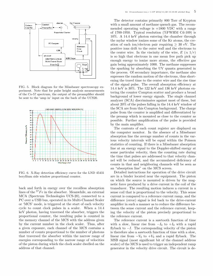
Figure 5 is a schematic of the experimental arrange-ment. A beryllium side window proportional gas counter(LND Model 45431, see Melissinos, p 181) and associ-ated measurement chain are used to selectively detectthe 14.4 keV photons emitted by excited 57Fe nucleiproduced by the beta decay of 57Co in a specially pre-pared “Mossbauer” source (i.e. 57Co diffused into a plat-inum substrate). An efficiency curve for the proportionalcounter is shown in Figure 6. Some of the 14.4 keVphotons are emitted by nuclei that share the recoil mo-mentum with macroscopic bits of the matter in whichthey are imbedded (“recoilless emission”) with the resultthat their fractional spread in energy, or line width, ∆E

E ,

is extraordinarily narrow, of the order of 10−12.A sample containing 57Fe atoms in an environment

that permits recoilless absorption of 14.4 keV photons, isplaced between the source and the proportional counter.The source is mounted on a piston which moves back andforth with a velocity that is a periodic sawtooth functionof time. This motion causes a corresponding sawtoothDoppler shift in the energies of the photons that traversethe sample. In effect, the narrow emission line is swept


FIG. 5. Block diagram for the Mossbauer spectroscopy ex-periment. Note that for pulse height analysis measurementsof the Co-57 spectrum, the output of the preamplifier shouldbe sent to the ‘amp in’ input on the back of the UCS20.

FIG. 6. X-Ray detection efficiency curve for the LND 45431beryllium side window proportional counter.

back and forth in energy over the recoilless absorptionlines of the 57Fe in the absorber. Meanwhile, an externalMCA (Spectrum Technologies UCS-20), connected to aPC over a USB bus, operated in its Multi-Channel Scaleror ‘MCS’ mode, is triggered at the start of each velocitycycle to count clock pulses in a scaler. When a 14.4keV photon, having traversed the absorber, triggers theproportional counter, the resulting pulse is counted inthe memory channel of the MCS with the address givenby the current number in the clock scaler. Thus, aftera given exposure, each channel of the MCS contains anumber of counts proportional to the number of photonsthat traversed the absorber within the narrow range ofenergies corresponding to the narrow range of velocitiesof the piston during which the clock scaler dwelled on theaddress of that channel.

The detector contains primarily 800 Torr of Kryptonwith a small amount of methane quench gas. The recom-mended operating voltage is +1800 VDC with a rangeof 1700-1950. Typical resolution (%FWHM Cd-109) is10%. A 14.4 keV photon entering the chamber throughthe mylar window ionizes some of the Kr atoms, the cre-ation of each ion/electron pair requiring ≥ 30 eV. Thepositive ions drift to the outer wall and the electrons tothe center wire. In the viscinity of the wire, E (∝ 1/r)is so high that electrons in one mean free path pick upenough energy to ionize more atoms, the effective gasgain being approximately 1000. The methane suppressesthe sparking by absorbing the UV quanta generated inthe process. Of secondary importance, the methane alsosupresses the random motion of the electrons, thus short-ening the travel time to the center wire and the rise timeof the signal pulse. The overall absorption efficiency at14.4 keV is 30%. The 122 keV and 136 keV photons en-tering the counter Compton scatter and produce a broadbackground of lower energy signals. The single channelanalyzer (SCA) discriminates against most of these, butabout 20% of the pulses falling in the 14.4 keV window ofthe SCA are from this Compton background. The chargepulse from the counter is amplified and differentiated bythe preamp which is mounted as close to the counter aspossible. Further amplification of the pulse is providedby the main amplifier.

The contents of each count register are displayed onthe computer monitor. In the absence of a Mossbauerabsorption line the average number of counts in the var-ious velocity intervals will be equal within the Poissonstatistics of counting. If there is a Mossbauer absorptionline at an energy equal to the Doppler-shifted energy atsome particular velocity, then the counting rate duringthe time that pulses are addressed to that velocity chan-nel will be reduced, and the accumulated deficiency ofcounts in that and neighboring channels will be seen asan “absorption line” on the MCS screen.

Detailed instructions for operation of the drive circuitare in a binder located near the equipment. The pistonon which the source is mounted is driven by the mag-netic force produced by a drive current in the coil of thetransducer. The resulting motion induces a current in asense coil that is proportional to the velocity. This sensecurrent is compared to a reference current ramp, and thedifference (error) signal is fed back to the drive-currentamplifier in such a manner as to reduce the difference be-tween the sense current and the reference current, keep-ing the velocity of the piston precisely proportional tothe reference current.

The reference current is a sawtooth function of timewith a slow, linear rise from −I0 to +I0 with a rapidflyback to −I. The corresponding velocity of the pistonis therefore also a sawtooth function of time with a slow,linear rise from −V0 to +V0 and a rapid flyback. TheMSB signal (most significant bit of the channel addressscaler) of the MCS is used to trigger an independent rampgenerator in the velocity drive circuit. The circuit is de-


signed for a nominal trigger rate of 6 Hz; it functionssatisfactorily at ≈ 5 Hz which is the closest rate that canbe obtained from the MCA with the thumb wheels set at[2] and [2]: (200 µs per channel). It is essential that thissetting be used. The thumb wheel on the Austin driveadjusts the amplitude of the motion, and hence, with thefixed frequency, the amplitude of the velocity sweep (therotary switch just below the thumb wheel is not used).

Display both the drive and velocity signals on an os-cilloscope and check that 1) the velocity ramp is linearand 2) the drive signal has an average value near zeroand is not in high frequency oscillation. The gain in theservo feedback loop, controlled by the FIDELITY knob,should be adjusted to achieve a linear velocity ramp.Start with the knob in the fully Counter-Clockwise po-sition and then cautiously increase until you hear a highpitched tone or until the DRIVE signal begins to oscil-late at about 12 kHz. Then, back it off slightly. If youhear a sound emanating from the drive motor, the gainis way too high. The D.C. component should be zero (ornearly so), both on the oscilloscope and as seen on thetwo LED’s just below and on either side of the velocitythumbwheel switch. The COMP. AMP.0 adjustment (oneither front panel or on the top of the unit) is used to zeroout the D.C. component. At lower velocities, both LED’swill be off when adjusted properly. The proper setting ofthe FIDELITY control is essential to obtaining good andreproducible Mossbauer spectra. There should be a slightringing after each point in the DRIVE waveform wherethe sense of the acceleration changes, but this should dieout rapidly. The ASYM UL potentiometer control onthe top of the unit is used for the flyback generator andshould be set for the best straight VELOCITY waveform.

1. Caution #0: If anything requires adjust-ment such as changing the thumbwheels toadjust the velocity range, or even if you sim-ply wish to erase the MCS spectrum (clear-ing the spectrum reinitializes the bistableMSB output) from the software interface, besure to turn off the MOTOR switch and turnoff the software before making the change.Wait about 30 seconds before turning on themotor switch. This allows the unit to stabi-lize after the bistable has been removed andreapplied.

2. Caution #1: The motor switch on the elec-tronic drive generator should be ON onlywhen the MCS is in the ‘acquire’ mode sothe motors are receiving proper ramp volt-ages.

3. Caution #2: Do not touch the fragile win-dow on the proportional counter detector.

FIG. 7. Typical Co-57 pulse height spectrum acquired by theSpectech UCS-20 multi-channel analyzer. Distance betweenCo-57 and proportional counter detector window is ∼10cm.Integration time = 100s. Co-57 had ∼5mCi of activity.

III.1. Mossbauer Start-Up Check List

1. Setup the apparatus as shown in Figure 5.

2. Turn on the power switch of the electronics rackand adjust the thumb wheels on the Mossbauerdrive to 80. Place the knob marked “Fidelity” inroughtly the central position. (leave the Mossbauerdrive switch in OFF position). Turn on the powerswitch to the SPECTECH UCS-20 Universal Com-puter Spectrometer.

3. Run the UCS20 Software from the adjacent Win-dows XP Computer desktop.

4. Use the software menu bar (Settings –Amp/HV/ADC) to turn on the high voltagebias to the propotional counter at +1800 VDC.Also set the conversion gain to 2048.

5. Set the Canberra 816 Amplifier gain to approxi-mately 20.

6. Remove any absorber present in the circular aper-ture between the Co-57 source and the proportionalcounter detector. Adjust the carriage holding thesource so that it is about 10 cm away from the de-tector window.

7. Run the MCA in pulse height analysis mode forabout 60 seconds and examine the resultant spec-trum. It should appear similar to Figure 7. Adjustthe gain controls so that the pulses in the strong6.4 keV iron K-line have an amplitude of about2.0 volts. Identify the fainter 14.4 keV Mossbauerline at about twice the amplitude of the iron K-line. Hint: a stack of papers roughly the size ofthis labguide will block the 6.4 keV line but passthe 14.4 keV line.


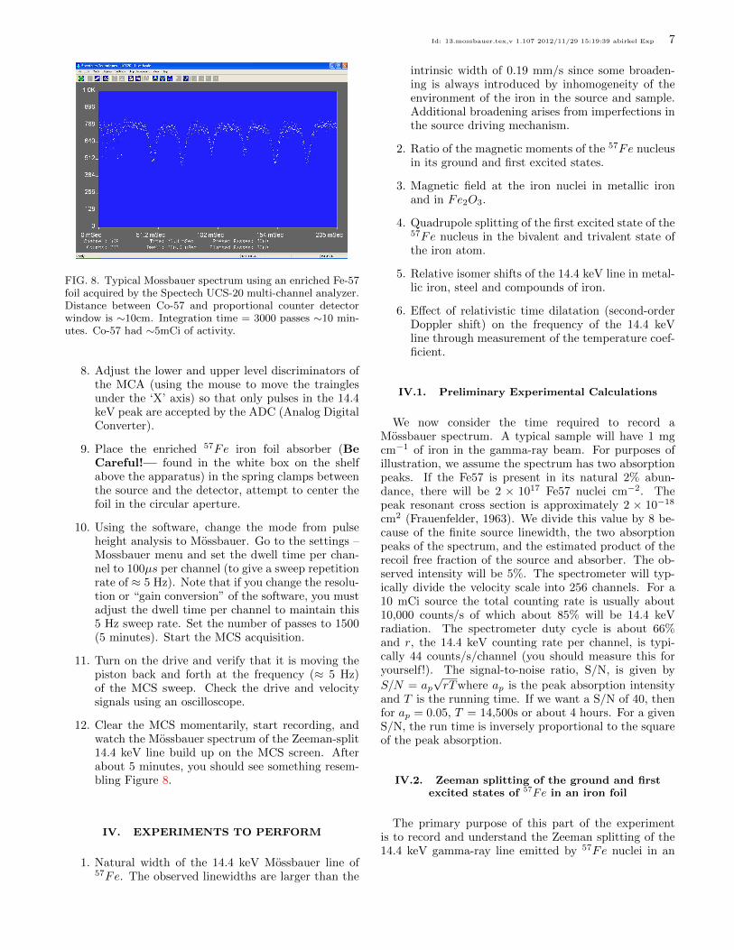
FIG. 8. Typical Mossbauer spectrum using an enriched Fe-57foil acquired by the Spectech UCS-20 multi-channel analyzer.Distance between Co-57 and proportional counter detectorwindow is ∼10cm. Integration time = 3000 passes ∼10 min-utes. Co-57 had ∼5mCi of activity.

8. Adjust the lower and upper level discriminators ofthe MCA (using the mouse to move the trainglesunder the ‘X’ axis) so that only pulses in the 14.4keV peak are accepted by the ADC (Analog DigitalConverter).

9. Place the enriched 57Fe iron foil absorber (BeCareful!— found in the white box on the shelfabove the apparatus) in the spring clamps betweenthe source and the detector, attempt to center thefoil in the circular aperture.

10. Using the software, change the mode from pulseheight analysis to Mossbauer. Go to the settings –Mossbauer menu and set the dwell time per chan-nel to 100µs per channel (to give a sweep repetitionrate of ≈ 5 Hz). Note that if you change the resolu-tion or “gain conversion” of the software, you mustadjust the dwell time per channel to maintain this5 Hz sweep rate. Set the number of passes to 1500(5 minutes). Start the MCS acquisition.

11. Turn on the drive and verify that it is moving thepiston back and forth at the frequency (≈ 5 Hz)of the MCS sweep. Check the drive and velocitysignals using an oscilloscope.

12. Clear the MCS momentarily, start recording, andwatch the Mossbauer spectrum of the Zeeman-split14.4 keV line build up on the MCS screen. Afterabout 5 minutes, you should see something resem-bling Figure 8.

IV. EXPERIMENTS TO PERFORM

1. Natural width of the 14.4 keV Mossbauer line of57Fe. The observed linewidths are larger than the

intrinsic width of 0.19 mm/s since some broaden-ing is always introduced by inhomogeneity of theenvironment of the iron in the source and sample.Additional broadening arises from imperfections inthe source driving mechanism.

2. Ratio of the magnetic moments of the 57Fe nucleusin its ground and first excited states.

3. Magnetic field at the iron nuclei in metallic ironand in Fe2O3.

4. Quadrupole splitting of the first excited state of the57Fe nucleus in the bivalent and trivalent state ofthe iron atom.

5. Relative isomer shifts of the 14.4 keV line in metal-lic iron, steel and compounds of iron.

6. Effect of relativistic time dilatation (second-orderDoppler shift) on the frequency of the 14.4 keVline through measurement of the temperature coef-ficient.

IV.1. Preliminary Experimental Calculations

We now consider the time required to record aMossbauer spectrum. A typical sample will have 1 mgcm−1 of iron in the gamma-ray beam. For purposes ofillustration, we assume the spectrum has two absorptionpeaks. If the Fe57 is present in its natural 2% abun-dance, there will be 2 × 1017 Fe57 nuclei cm−2. Thepeak resonant cross section is approximately 2 × 10−18

cm2 (Frauenfelder, 1963). We divide this value by 8 be-cause of the finite source linewidth, the two absorptionpeaks of the spectrum, and the estimated product of therecoil free fraction of the source and absorber. The ob-served intensity will be 5%. The spectrometer will typ-ically divide the velocity scale into 256 channels. For a10 mCi source the total counting rate is usually about10,000 counts/s of which about 85% will be 14.4 keVradiation. The spectrometer duty cycle is about 66%and r, the 14.4 keV counting rate per channel, is typi-cally 44 counts/s/channel (you should measure this foryourself!). The signal-to-noise ratio, S/N, is given by

S/N = ap√rTwhere ap is the peak absorption intensity

and T is the running time. If we want a S/N of 40, thenfor ap = 0.05, T = 14,500s or about 4 hours. For a givenS/N, the run time is inversely proportional to the squareof the peak absorption.

IV.2. Zeeman splitting of the ground and firstexcited states of 57Fe in an iron foil

The primary purpose of this part of the experimentis to record and understand the Zeeman splitting of the14.4 keV gamma-ray line emitted by 57Fe nuclei in an


iron foil. The other purpose is to establish a convenientsecondary calibration standard.

Record the absorption spectrum for a sufficient timeto obtain at least several thousand counts per channel sothat you can measure accurate centroid values, intensi-ties, and shapes of the six lines of the pattern. Measurethe channel positions of each of the absorption peaks inthe MCS display.

Next, without changing any of the settings, carry outan absolute calibration of the drive motion with the in-terferometer, as described below. Derive from your mea-sured spectrum and the velocity calibration data the sep-aration in velocity (mm/s) between adjacent pairs of linesin the six-line Zeeman pattern. With these results inhand you can use the quickly observable Zeeman patternof the enriched iron foil as a secondary calibration stan-dard for each of your subsequent Mossbauer spectrummeasurements.

Convert the velocity separations between the lines ofthe Zeeman pattern into energy separations. The mag-netic moment of the ground state of 57Fe has been mea-sured by electron spin resonance techniques to be 0.0903± 0.0007 µN . Using this fact, and interpreting the Zee-man pattern in terms of the energy level diagram (seeMelissinos, p. 277), determine the internal magnetic fieldat a nucleus of iron in the iron foil absorber, and the mag-netic moment of the first excited state. Discuss the ex-perimental errors in the values you have obtained. Withthe data in hand can you verify the discovery of Hanna etal. (1960) [5] that the magnetic moments of the groundand first excited states have opposite signs?

IV.3. Absolute calibration

Calibration of the velocity sweep is accomplished withthe aid of a Michelson interferometer shown schemati-cally in Fig. 9. A beam of coherent light from a laseris split by partial reflection from a glass slide oriented at45◦ so that the two parts traverse different paths beforestriking the same spot on a photodiode. While the lengthof one path is fixed, the length of the other path variesbecause it includes a reflection from a mirror mountedon the moving piston. When the piston moves a distanceequal to one-half of the wavelength of the laser light, thelength of the path increases by one wave length, the phaseof the beam at the photodiode changes by 360◦, and theintensity of the recombined beam at the photodiode goesthrough one cycle of constructive and destructive inter-ference. Every cycle of interference produces one cycleof a sinusoidal voltage signal from the photodiode thatcan be registered as one pulse by the multichannel scaler.Call Vi the average velocity of the moving mirror duringthe time interval corresponding to the ith channel of themultichannel scaler display. The average rate of pulsesduring the ith time interval is 2Vi

λ . If we call T the timeinterval during which pulses are directed to a given chan-nel by the clock register, i.e., the dwell time per channel,

Photodiode

Laser Fixed mirror

Moving mirror

Source

Proportional Counter

Sample

Drive Motor

EG&G Amplifier AC-1S Coupled

Gain = 25-100, DC-300kHz Filterto LeCroy Gate Generator 222 to External MCS Input on UCS-20 Run UCS-20 Software in External Mossbauer Mode

MCS quality input (2.5 VDC, > 150ns)

to Lecroy Discriminator 623B

FIG. 9. Schematic diagram of the Michelson interferome-ter for calibration of the velocity sweep. Be particularlysensitive to try and block any stray reflections of theHeNe laser from interferometer into another anotherportion of the lab. Block as necessary using blackposterboard or index cards.

and N the number of sweeps made during the course of acalibration run, then the total number of counts recordedin the ith channel will be:

C = NT(2Viλ

). (8)

Solving for the velocity corresponding to the ith chan-nel, we find:

Vi =Cλ

2NT. (9)

The orientations of the laser, the beam splitter (glassslide), and the two adjustable mirrors should be adjustedso that the incident and reflected beams all strike thebeam splitter as close to the same spot as possible with-out allowing a reflected beam to go straight back intothe laser where it may disrupt the performance of thelaser. Be sure to prevent unwanted laser lightfrom crossing the room potentially harming an-other investigator. Adjust the mirrors to superposethe two beams of the interferometer on the photodiode.

Operate the UCS20 in ‘External Mossbauer’ mode andturn on the Mossbauer drive motor. Watch the oscillo-scope for the interference signal as you make small ad-justments of the mirrors. When you see some interfer-ence fringes on the photodiode output, send the signalto the EG&G 5113 Amplifier with a gain of about 10-100 and AC couple the A-input. Apply a low-pass filterwith a cutoff of about 300 kHz. This signal is then sentto the LeCroy 623B discriminator converting the analoginterference signal into a fast rise time logic level pulse.In order to generate an “MCS-friendly” input, we pro-cess the output of the discriminator with the LeCroy 222Gate Generator. Set the pulse width to 10 microsec-onds and send the TTL output into the External MCSinput on the back of the Spectrum Techniques UCS-20


-V 0 +V

FIG. 10. Ideal appearance of the multichannel scaler screenafter several minutes of operation with the interferometer ve-locity calibrator. The sharp feature at the start is producedduring the rapid reversal of the velocity of the piston at thehigh speed end of its stroke. In reality, the bottom of the “V”will probably be truncated due to the low amplitude of thepulses during the low-velocity portion of the sweep.

instrument. When everything is working properly, themultichannel scaler look similar to Fig. 10.

When you have mastered the calibration procedure,run the Mossbauer setup with an enriched iron foil ab-sorber and adjust the amplitude of the velocity sweep toobtain the 6-line Zeeman pattern that will be your sec-ondary calibrator. Record the channel numbers of theabsorption line centroids. Without changing any of thesettings of the Mossbauer drive circuit except to turnit off and on, proceed with the interferometer calibra-tion by replacing the proportional counter pulses withthe interferometer pulses. If everything is working prop-erly, the velocity sweep should be precisely linear so thatVi = ai + b where ‘a’ and ‘b’ are constants. Thus twomeasurements of the velocity in good (smooth) portionsof the calibration “V” pattern are sufficient to determine‘a’ and ‘b’. Since realigning the interferometer each timea velocity change is made, subsequent velocity calibra-tions may be made using the known splittings of eithermetallic iron or Fe2O3. Please see the ‘ASA-700 Moss-bauer Drive’ document under the ‘Selected Resources’section of the Junior Lab web site for these data.

The following is a menu of possible investigations:

1. Properties of the Resonant Line Shape. In this ex-periment, you will use an absorber of sodium ferro-cyanide Na3Fe(CN)6 · 10H2O which has no mag-netic field or electric field gradient at the crystalsites of the iron nuclei. Absorbers of three differentthicknesses are available. This allows you to mea-sure the line width as a function of thickness so thatyou can extrapolate your results to zero thickness.Derive a value for the intrinsic width of the 14.4keV first excited state of 57Fe and compute theimplied lifetime of the excited state. What other

causes of line broadening may be present in yourdata?

2. Temperature coefficient of the Mossbauer lines andthe twin “paradox”. The temperature effect is ashift in the resonant frequency of an absorptionline due to the second order Doppler effect whichamounts to a slowing of the atomic “clocks” in aheated sample due to their thermal motion relativeto the reference atomic clocks in the lab. Accord-ing to the theory of relativity, the effect should beof the order of (vc )2 ≈ kT

mc2 ≈ 10−13. That is smallindeed, but accessible to Mossbauer spectroscopy.It is also a proof that the so-called “twin paradox”(not really a paradox since it follows logically fromthe theory of relativity) is really true, i.e. that ifyou send your twin on a fast round trip rocket flighthe/she will return younger than you. See Reference[4], page 63 for more details. The strategy of thisexperiment is as follows:

(a) Operate the spectrometer at very high disper-sion and calibrate it by measuring the separa-tion between the two central peaks of the 57Fespectrum;

(b) Measure the fractional shift position ∆EE of

the single peak of stainless steel between roomtemperature T and T + ∆T ;

(c) Compare the result with the theory of Joseph-son (page 252 within the Frauenfelder collec-tion).

To measure the temperature effect reduce the ve-locity amplitude of the Mossbauer drive so that thetwo central components of the Zeeman pattern arewidely separated, say by 400 channels, i.e. increasethe dispersion of the spectrometer so that the smalleffect of temperature will be able to cause a shiftof several channels in the centroids of the Zeemanlines. Calibrate the velocity scale by recording thelocations of the central two peaks of the 57Fe spec-trum. Place the aluminum-block oven with the My-lar windows, containing the thin stainless steel andattached heater and thermocouple, in position be-tween source and counter. Accumulate a spectrumwith sufficient counts so that the positions of thepeaks of the absorption line can be determined withan uncertainty no greater than 11 channel.. Ad-just the temperature control to 120◦C and turn onthe heater. When the temperature has stabilizedrecord a high-temperature spectrum. Repeat coldand hot measurements several times to reduce andevaluate your random error. Determine the tem-perature coefficient from your data, i.e. the frac-tional change in the peak energies per degree centi-grade, and compare your results with the theoret-ical prediction (see the discussion in Frauenfelder,1962, page 63).


3. Quadrupole splitting and isomer shifts in Fe++ andFe+++ ions. Measure the absorption spectra insamples of FeSO4 · 7H2O and Fe2(SO4)3 and de-termine the quadrupole splittings (if any) and theisomer shifts. Accumulations of 30 to 60 minutesshould be sufficient to show the absorption spectraand permit accurate measurement of the splittings.See [6] for a discussion of the implications of suchmeasurements.

4. Combined Zeeman and quadrupole effects inFe2O3. Measure the absorption spectrum of anisotope-enriched sample of red (ferrous) iron ox-ide, Fe2O3. (Note that the red oxide, otherwiseknown as rust, is not ferromagnetic, i.e. it is notattracted by a magnet.) Allowing for the combinedeffects of Zeeman and quadrupole splitting, and us-ing the value for the magnetic moment of the firstexcited state obtained above, derive the strength ofthe magnetic field at the iron nuclei in red oxide,and the magnitude of the product of the quadrupole

moment and the electric field gradient.

5. The absorption spectrum of magnetite (Fe3O4;the black magnetic oxide of iron). Try to fig-ure out what is going on. The available samplesof magnetite require long exposures because theyhave only the natural abundance of 2%. TheMossbauer spectrum of magnetite has provided im-portant clues to the structure of this peculiarlycomplex substance. You will probably need to diginto the literature for help in the interpretation ofthe spectrum. There is an extensive series of re-views on Mossbauer spectroscopy in the ScienceLibrary. Incidentally, the black sand that you mayhave seen on ocean beaches is magnetite.

6. Other iron-bearing materials, like rust, cast ironfilings, spring steel, medicinal iron pills, black sand.

Other references related to this experiment are [7–12]

[1] Nobel Lectures from Robert Hofstadter and Rudolph Lud-wig Mossbauer .

[2] A. C. Melissinos, Experiments in Modern Physics (Aca-demic Press: Orlando, 2003) ISBN QC33.M523, physicsDepartment Reading Room.

[3] S. Gasiorowicz, Quantum Physics, 2nd ed. (Wiley: NewYork, 1996) ISBN QC174.12.G37, physics DepartmentReading Room.

[4] H. Frauenfelder, The Mossbauer Effect (Benjamin: NewYork, 1962) ISBN QC477.F845, physics DepartmentReading Room.

[5] S. S. Hanna, J. Heberle, C. Littlejohn, G. J. Perlow, R. S.Preston, and D. H. Vincent, Phys. Rev. Letters 4, 177(1960).

[6] S. DeBenedetti, Sci. Amer.(1960).[7] Boyle and Hall, Reports on Progress in Physics, XXV

Aug, 442 (1962), qC.R425, Science Library Journal Col-lection, London.

[8] O. C. Kistner and A. N. Sunyar, Phys. Rev. Letters 4,412 (1960).

[9] O. C. Kistner, A. N. Sunyar, and D. H. Vincent, Ameri-can Institute of Physics: New York(1963).

[10] S. L. Ruby, L. M. Epstein, and K. H. Sun, Rev. Sci. Instr.31, 580 (1960), qC.R453, Physics Department ReadingRoom.

[11] E. Oldfield and R. Kirkpatrick, Science 227, 1537 (1985).[12] U. Gonser, Mossbauer Spectroscopy, Topics in Applied

Physics, Vol. 5 (Springer-Verlag, 1975) ISBN QC491.M6,pp 16-17.

Model Description Source

ASA S-700A Mossbauer Drive NA

ASA K-4 Mossbauer Motor NA

ASA PC-200 Scintillator no longer available

Canberra 3002D HV Power Supply canberra.com

Canberra 815 Amplifier canberra.com

MG 05-LHR-111 Laser mellesgriot.com

Ortec 109PC Pre-Amp. ortec-online.com

MIT Low Freq Amp homemade

MIT Interferometer Setup homemade

MIT St. Steel Absorber/Oven homemade

MIT Mossbauer Absorbers webres.com

Appendix A: Mosssbuaer Effect Equipment List

Appendix B: Verification of Velocity Calibration

To first order, T , the dwell time per channel is simplythat which was set under the Mossbauer settings sub-menu in the UCS-20 software.

This can be confirmed, if desired by feeding pulses froma pulse generator to both the input of the pulse ampli-fier and to a frequency meter. Integrate for sufficienttime to obtain a smooth horizontal pattern and countthe number of sweeps. From the number of sweeps, theaverage number of pulses recorded per channel, and thefrequency of the pulses, you can compute T , the dwelltime per channel.

Example: Suppose you recordN=1000 sweeps and findC=2000 counts in a particular channel. With the ASA-


700 thumb-wheel sweep controls set at 80 mm s−1, youmay have found in the frequency-generator calibrationthat T=170µs ch−1. The wavelength of the HeNe laserlight is λ = 6328A, or 6.328 × 10−5cm. According toEquation 9, the piston velocity at that part of the cycleis

V =6.328× 10−5 × 2000

1000× 0.000170× 2= 0.367 cm s−1 (B1)


FIG. 11. From Mossbauer Spectroscopy, Edited by U. Gonser, Springer-Verlag, 1975

m ossbauer spectroscopy - mitweb.mit.edu/8.13/www/jlexperiments/jlexp13.pdf · with the germanium...

Documents