m-estimators with applications to hypothesis testing for

asymptotic normality of nonparametric

M-estimators with applications to

hypothesis testing for panel count data

Xingqiu Zhao and Ying Zhang

The Hong Kong Polytechnic University and Indiana University

Abstract: In semiparametric and nonparametric statistical inference, the asymptotic nor-

mality of estimators has been widely established when they are√n-consistent. In many

applications, nonparametric estimators are not able to achieve this rate. We have a result

on the asymptotic normality of nonparametric M -estimators that can be used if the rate

of convergence of an estimator is n−1/2 or slower. We apply this to study the asymptotic

distribution of sieve estimators of functionals of a mean function from a counting process,

and develop nonparametric tests for the problem of treatment comparison with panel count

data. The test statistics are constructed with spline likelihood estimators instead of non-

parametric likelihood estimators. The new tests have a more general and simpler structure

and are easy to implement. Simulation studies show that the proposed tests perform well

even for small sample sizes. We find that a new test is always powerful for all the situations

considered and is thus robust. For illustration, a data analysis example is provided.

Key words and phrases: Asymptotic normality; M -estimators; Nonparametric maximum

likelihood; Nonparametric maximum pseudo-likelihood; Nonparametric tests; Spline.

Statistica Sinica: Preprintdoi:10.5705/ss.202014.0021

___________________________________________________________________

This is the author's manuscript of the article published in final edited form as:

Zhao, X., & Zhang, Y. (2017). Asymptotic normality of nonparametric M-estimators with applications to hypothesis testing for panel count data. Statistica Sinica, 27(2), 931–950. https://doi.org/10.5705/ss.202014.0021

https://doi.org/10.5705/ss.202014.0021

1 Introduction

Weak convergence theory and empirical theory (van der Vaart and Wellner (1996)) have been

widely used to study the asymptotic properties of estimators in semiparametric and nonpara-

metric models. When the convergence rate of estimators is n−1/2, the asymptotic distribution

of the estimators can be derived by using the weak convergence theorem on Z-estimators

(van der Vaart and Wellner (1996, page 310)). For example, Zeng, Lin, and Yin (2005) and

Zeng and Lin (2006, 2007) obtained the desired asymptotic normality of the estimators for

the proportional odds model and the semiparametric transformation models by verifying the

conditions of Theorem 3.3.1 of van der Vaart and Wellner (1996). When the convergence

rate is slower than n−1/2, for example, the convergence rates of nonparametric maximum

likelihood estimators of cumulative distribution functions based on interval-censored data

are n−1/3 (Groeneboom and Wellner (1992)), this theorem is no longer applicable. For such

situations, it is difficult to derive the asymptotic distribution of nonparametric estimators.

Zhang (2006) and Balakrishnan and Zhao (2009) investigated the asymptotic normality of

functionals of the nonparametric maximum pseudo-likelihood and likelihood estimators for

panel count data. We have a general theorem dealing with the asymptotic normality of non-

parametric M -estimators and we apply this to panel count models as illustrative examples.

For the nonparametric inference of panel count data, several estimation and testing meth-

ods have been developed. Sun and Kalbfeisch (1995), Wellner and Zhang (2000), Lu, Zhang,

and Huang (2007), and Hu, Lagakos, and Lockhart (2009a, b) studied the nonparametric

estimation of the mean function of the underlying counting process with panel count data by

using isotonic regression techniques, the likelihood approach, the spline likelihood approach,

2

Statistica Sinica: Preprint doi:10.5705/ss.202014.0021

the estimating equation approach, and the generalized least squares method, respectively;

Thall and Lachin (1988), Sun and Fang (2003), Zhang (2006), and Balakrishnan and Zhao

(2009) presented some nonparametric tests for nonparametric comparison of mean function

of counting process with panel count data. For a comprehensive review about the analysis

of panel count data, see Sun and Zhao (2013).

Lu, Zhang, and Huang (2007, 2009) showed that the spline likelihood estimators have

a convergence rate slower than n−1/2 but faster than n−1/3, and are more efficient both

statistically and computationally than the nonparametric maximum likelihood estimators in

simulations. In this paper, we explore asymptotic normality of functionals of spline likelihood

estimators of mean functions, and propose some new nonparametric tests based on them to

compare with existing tests for the nonparametric comparison of counting processes with

panel count data.

The remainder of the article is organized as follows. In Section 2, we present a general

theorem regarding the asymptotic normality of nonparametric M -estimators. In Section 3,

we briefly review the nonparametric spline-based likelihood estimators for panel count data

and establish the asymptotic normality of their functionals. Section 4 presents two classes of

nonparametric test statistics for comparing two treatment groups with respect to their mean

functions. The asymptotic normality of the proposed test statistics are established. Section

5 reports some simulation results to assess the finite-sample properties of the proposed

test procedure and to compare them with the tests based on the nonparametric likelihood

estimators. A data analysis example is provided in Section 6. Section 7 contains some

concluding remarks. The proofs of theorems are given in the Supplementary Materials

available at the Statistica Sinica journal website.

3


2 Asymptotic Distributional Theory of Nonparametric

M-Estimators

Suppose X = (X1, . . . , Xn) is a random sample taken from the distribution of X, and

ln(Λ;X) =∑n

i=1m(Λ;Xi) is an objective function based on X, where Λ is an unknown

function in the class F . Let Fn be the sieve parameter space satisfying

Fn ⊆ Fn+1 ⊆ · · · ⊆ F , forn ≥ 1.

Assume that Λn is the estimator of Λ0 that maximizes ln(Λ;X) with respect to Fn.

Suppose Λη is a parametric path in F through Λ, Λη ∈ F and Λη|η=0 = Λ. Let H = {h :

h = ∂Λη∂η|η=0} and l∞(H) be the space of bounded functionals on H under the supermum

norm ||f ||∞ = suph∈H |f(h)|. For h ∈ H, we define a sequence of maps Gn of a neighborhood

of Λ0, denoted by U , in the parameter space for Λ into l∞(H) by

Gn(Λ)[h] = n−1 ∂

∂ηln(Λη;X)|η=0

= n−1

n∑i=1

∂

∂ηm(Λη;Xi)|η=0

≡ Pnψ(Λ;X)[h],

and take G(Λ)[h] = Pψ(Λ;X)[h], where P and Pn denote the probability measure and

empirical measure with Pf =∫fdP and Pnf = n−1

∑ni=1 f(Xi), respectively.

To establish the asymptotic normality, we need the following conditions.

A1.√n(Gn −G)(Λn)[h]−

√n(Gn −G)(Λ0)[h] = op(1).

A2. G(Λ0)[h] = 0 and Gn(Λn)[h] = op(n−1/2).

4


A3.√n(Gn −G)(Λ0)[h] converges in distribution to a tight Gaussian process on l∞(Hr).

A4. G(Λ)[h] is Frechet-differentiable at Λ0 with a continuous derivative GΛ0 [h].

A5. G(Λn)[h]−G(Λ0)[h]− GΛ0(Λn − Λ0)[h] = op(n−1/2).

Theorem 2.1 If A1-A5 hold, then for any h ∈ H,

−√nGΛ0(Λn − Λ0)[h] =

√n(Gn −G)(Λ0)[h] + op(1).

Remark 1. The above theorem does not require the Λn be√n-consistent, while the

conditions stated in Theorem 3.3.1 of van der Vaart and Wellner (1996) imply that the

estimator has the usual convergence rate n−1/2.

Remark 2. Assumptions A2-A4 are the analytical conditions given in Theorem 3.3.1

of van der Vaart and Wellner (1996). Assumptions A1 and A5 require the remainder in a

Taylor expansion be negligible; they are weaker than those required by van der Vaart and

Wellner (1996).

The theorem can be widely used to establish the asymptotic normality of nonparametric

estimators no matter whether the rate of convergence is n−1/2, or is slower. We focus on

counting process models with panel count data to illustrate applications of the theorem.

5


3 Asymptotic Normality of Functionals of Nonpara-

metric Spline-based Likelihood Estimators for Panel

Count Data

3.1 Nonparametric Spline-based Likelihood Estimation

Consider a recurrent event study that consists of n independent subjects and let Ni(t) denote

the number of occurrences of the recurrent event of interest before or at time t for subject i.

For subject i, suppose that Ni(·) is observed only at finite time points TKi,1 < · · · < TKi,Ki ≤

τ , where Ki denotes the potential number of observation times, i = 1, . . . , n, and τ is the

length of the study.

In the following, we assume that (Ki;TKi,1, ..., TKi,Ki) are independent of the counting pro-

cessesNi’s. Let X = (K,T,N), where T = (TK,1, ..., TK,K) and N = (N(TK,1), . . . , N(TK,K)).

Then {Xi = (Ki,Ti,Ni), i = 1, ..., n} is a random sample of size n from the distribution of

X, where Ti = (TKi,1, ..., TKi,Ki) and Ni = (Ni(TKi,1), . . . , Ni(TKi,Ki)).

Suppose that for each subject, Ni(t) is a non-homogeneous Poisson process with the mean

function Λ(t). The log pseudo-likelihood and the log-likelihood functions for Λ are

lpsn (Λ) =n∑i=1

Ki∑j=1

[Ni(TKi,j) log {Λ(TKi,j)} − Λ(TKi,j)] ,

ln(Λ) =n∑i=1

Ki∑j=1

[∆Ni(TKi,j) log {∆Λ(TKi,j)} −∆Λ(TKi,j)] ,

after omitting the parts independent of Λ, where TKi,0 = 0, ∆Λ(TKi,j) = Λ(TKi,j) −

6


Λ(TKi,j−1), and ∆Ni(TKi,j) = Ni(TKi,j)−Ni(TKi,j−1).

For estimation of the smooth function Λ0(t), we use B-spline function approximation (Lu,

Zhang, and Huang (2007)). Let T = {si, i = 1, . . . ,mn + 2l}, with

τ0 = s1 = · · · = sl < sl+1 < · · · < smn+l < smn+l+1 = · · · = smn+2l = τ,

be a sequence of knots that partition [τ0, τ ] into mn + 1 subintervals Ii = [sl+i, sl+i+1], for

i = 0, 1, . . . ,mn. Let Φn be the class of polynomial splines of order l ≥ 1 with the knot

sequence T . Then Φn can be linearly spanned by the normalized B-spline basis functions

{Bi, i = 1, . . . , αqn} with qn = mn + l (Schumaker (1981)). Define a subclass of Φn,

Ψn =

{qn∑i=1

αiBi : 0 ≤ α1 ≤ · · · ≤ αqn

}.

Following Lu, Zhang and Huang (2007), the estimators Λpsn and Λn are the values that

maximize lpsn (Λ) and ln(Λ) with respect to Λ ∈ Ψn, respectively.

We denote the spline pseudo-likelihood and spline likelihood estimators of Λ by Λpsn =∑qn

i=1 αpsinBi and Λn =

∑qni=1 αinBi.

3.2 Asymptotic Normality

Let B denote the collection of Borel sets in R, and let B[0,τ ] = {B∩ [0, τ ] : B ∈ B}. Following

Wellner and Zhang (2000), define measures µ1 and µ2 as follows: for B,B1, B2 ∈ B[0,τ ],

µ1(B) =∞∑k=1

P (K = k)k∑j=1

P (Tk,j ∈ B|K = k)

= E

{K∑j=1

I(TK,j ∈ B)

},

7


µ2(B1 ×B2) =∞∑k=1

{P (K = k)k∑j=1

P (Tk,j−1 ∈ B1, Tk,j ∈ B2|K = k)}

= E

{K∑j=1

I(TK,j−1 ∈ B1, TK,j ∈ B2)

}.

Define the L2-metrics d1 and d2 as

d1(Λ1,Λ2) =

{∫|Λ1(t)− Λ2(t)|2dµ1(t)

}1/2

,

d2(Λ1,Λ2) =

{∫ ∫|(Λ1(u)− Λ1(v))− (Λ2(u)− Λ2(v))|2dµ2(u, v)

}1/2

.

To establish the asymptotic properties of the estimators, we need the following regularity

conditions.

C1. The maximum spacing of the knots, ∆ ≡ maxl+1≤i≤mn+l+1 |si − si−1| = O(n−v) with

mn = O(nv) for 0 < v < 0.5. There exists a constant M > 0 such that ∆/δ ≤ M

uniformly in n, where δ ≡ minl+1≤i≤mn+l+1 |si − si−1|.

C2. The true mean function Λ0 is a nondecreasing function over [0, τ ] with Λ(0) = 0, with

a bounded rth derivative in [0, τ ] for r ≥ 1, and Λ′0(t) ≥ a0 for some a0 ∈ (0,∞).

C3. There exists a positive integer K0 such that P (K ≤ K0)=1.

C4. For some positive constant k0, E[exp{k0N(τ)}] <∞.

C5. P (∩Kj=1{TK,j ∈ [τ0, τ ]}) = 1 with τ0 > 0, Λ0(τ0) > 0, and Λ0(τ) ≤M0 for some constant

M0 > 0.

C6. µ1(τ0) > 0, and for all τ0 < τ1 < τ2 < τ , µ1((τ1, τ2)) > 0.

C7. There exists a positive constant s0 such that P (min1≤j≤K{TK,j − TK,j−1} ≥ s0) = 1.

8


C8. µ1 is absolutely continuous with respect to Lebesgue measure, with derivative µ1.

C9. µ2 is absolutely continuous with respect to Lebesgue measure, with derivative µ2.

C10. If with probability 1, h(TK,j) = 0, j = 1, . . . , K for some h, then h = 0.

Conditions C1-C5 and C7 are required by Lu, Zhang and Huang (2007); condition C6 is

required by Balakrishnan and Zhao (2009). Conditions C8 and C9 are similar to C11 in

Wellner and Zhang (2007). Condition C10 is needed for identifiability of the model.

Theorem 3.1 Suppose C1-C6 and C10 hold, and let

Hr ={g(·) : |g(r−1)(s)− g(r−1)(t)| ≤ c0|s− t| for all τ0 ≤ s, t ≤ τ

}.

where g(r−1) is the (r − 1)th derivative function of g, and c0 is a constant.

(i) If C8 holds, then for h ∈ Hr,

√n

∫{Λps

n (t)− Λ0(t)}dh(t)→d N(0, σ2ps), (3.1)

where σ2ps is given at (S2.4) of Supplementary Materials.

(ii) If C7 and C9 hold, then for h ∈ Hr,

√n

∫{Λn(t)− Λ0(t)}dh(t)→d N(0, σ2), (3.2)

where σ2 is given at (S2.7) of Supplementary Materials.

Corollary 3.1 Suppose the conditions in Theorem 3.1 hold.

(i)

√n

∫h(t)

Λpsn (t)− Λ0(t)

Λ0(t)dµ1(t)→d N(0, σ2

1), (3.3)

9


where h ∈ Hr, and

σ21 = E

[K∑j=1

h(TK,j)N(TK,j)− Λ0(TK,j)

Λ0(TK,j)

]2

. (3.4)

(ii)

√n

∫{h(u)− h(v)}{Λn(u)− Λn(v)} − {Λ0(u)− Λ0(v)}

{Λ0(u)− Λ0(v)}dµ2(u, v)

→d N(0, σ22), (3.5)

where h ∈ Hr, and

σ22 = E

[K∑j=1

∆h(TK,j)∆N(TK,j)−∆Λ0(TK,j)

∆Λ0(TK,j)

]2

. (3.6)

Remark 3. These results can be used to construct new tests for the problem of multi-

sample nonparametric comparison of counting processes with panel count data.

Remark 4. We can show that under some regularity conditions, (3.1)-(3.6) hold for the

two nonparametric likelihood-based estimators proposed by Wellner and Zhang (2000).

4 Nonparametric Two-sample Tests

Consider a longitudinal study with some recurrent event and n independent subjects from

two groups, nl in the lth group with n1+n2 = n. LetNi(t) denote the counting process arising

from subject i and Λl(t) denote the mean function of the counting process corresponding to

group l, l = 1, 2. Here, the problem of interest is to test the null hypothesis H0 : Λ1(t) =

Λ2(t). Suppose subject i is observed only at distinct time points 0 < TKi,1 < · · · < TKi,Ki

and that no information is available about Ni(t) between them.

10


Let Λpsl and Λl denote the spline pseudo-likelihood and spline likelihood estimators of

Λl based on samples from all the subjects in the lth group. Let Λ0(t) denote the common

mean function of the Ni(t)’s under H0, and let Λps0 and Λ0 be the spline pseudo-likelihood

and spline likelihood estimators of Λ0 based on the pooled data. Clearly, µ1(t) and µ2(u, v)

can be consistently estimated by

µ1(t) =1

n

n∑i=1

Ki∑j=1

I(TKi,j ≤ t),

µ2(u, v) =1

n

n∑i=1

Ki∑j=1

I(TKi,j−1 ≤ v, TKi,j ≤ u),

respectively.

To test the hypothesis H0, Zhang (2006) and Balakrishnan and Zhao (2009) proposed to

use the two statistics

UZ =√n

∫ τ

0

Wn(t){Λ1,mple(t)− Λ2,mple(t)}dµ1(t),

UBZ =1√n

n∑i=1

[Ki−1∑j=1

Wn(TKi,j)Λ0,mle(TKi,j)

×

{(∆Λ1,mle(TKi,j+1)

∆Λ0,mle(TKi,j+1)− ∆Λ1,mle(TKi,j)

∆Λ0,mle(TKi,j)

)

−

(∆Λ2,mle(TKi,j+1)

∆Λ0,mle(TKi,j+1)− ∆Λ2,mle(TKi,j)

∆Λ0,mle(TKi,j)

)}+Wn(TKi,Ki)Λ0,mle(TKi,Ki)

×

{(1− ∆Λ1,mle(TKi,Ki)

∆Λ0,mle(TKi,Ki)

)−

(1− ∆Λ2,mle(TKi,Ki)

∆Λ0,mle(TKi,Ki)

)}],

where Wn(t) is a bounded weight process, Λl,mple and Λl,mle denote the maximum pseudo-

likelihood and maximum likelihood estimators of Λl based on samples from all the subjects

in the lth group, and Λ0,mle denotes the maximum likelihood estimator of Λ0 based on the

11


pooled data. We propose the two test statistics

Upsn =

√n

∫hpsn (t)

Λps1 (t)− Λps

2 (t)

Λps0 (t)

dµ1(t)

=1√n

n∑i=1

Ki∑j=1

hpsn (TKi,j)Λps

1 (TKi,j)− Λps2 (TKi,j)

Λps0 (TKi,j)

,

Un =√n

∫{hn(u)− hn(v)}{Λ1(u)− Λ1(v)} − {Λ2(u)− Λ2(v)}

{Λ0(u)− Λ0(v)}dµ2(u, v)

=1√n

n∑i=1

Ki∑j=1

{∆hn(TKi,j)}∆Λ1(TKi,j)−∆Λ2(TKi,j)

∆Λ0(TKi,j),

where hpsn (t) and hn(t) are bounded weight processes. For the propose of comparison, we

consider three choices of the weight processes hpsn (t) and hn(t): hpsn (t) = Λps0 (t)W

(k)n (t) and

hn(t) = Λ0(t)W(k)n (t), where W (1)(t) = 1, W

(2)n (t) =

∑ni=1 I(t ≤ TKi,Ki), and W

(3)n (t) =

1 − W(2)n (t) =

∑ni=1 I(t > TKi,Ki). Other choices of weight processes can be made. For

example, if we take hn(t) = {Λ0(t)}2, the structure of Upsn is similar to UZ , while the structure

of Un is much simpler than that of UBZ .

Theorem 4.1 Suppose the conditions of Theorem 3.1 hold. Suppose that hn(t)’s are

bounded weight processes and that there exists a bounded function h(t) such that h ∈ Hr, and[∫ τ

0

{hn(t) − h(t)}2 dµ1(t)

]1/2

= op(n− 1

2(1+2r) ) .

If n1/n → p as n→∞, where 0 < p < 1, then, under H0 : Λ1 = Λ2 = Λ0,

(i) Upsn has an asymptotic normal distribution N(0, σ2

ps), where

σ2ps =

(1

p+

1

1− p

)σ2

1

with σ21 as given as (3.4);

12


(ii) Un has an asymptotic normal distribution N(0, σ2), where

σ2 =

(1

p+

1

1− p

)σ2

2

with σ22 as given as (3.6);

(iii) If

max1≤i≤n

E

[Ki∑j=1

{hn(TKi,j)− h(TKi,j)}2

]−→ 0,

then σ21, σ

22 can be consistently estimated by

σ21 =

1

n

n∑i=1

[Ki∑j=1

hn(TKi,j)Ni(TKi,j)− Λps

0 (TKi,j)

Λps0 (TKi,j)

]2

,

σ22 =

1

n

n∑i=1

[Ki∑j=1

∆hn(TKi,j)∆Ni(TKi,j)−∆Λ0(TKi,j)

∆Λ0(TKi,j)

]2

, respectively.

Remark 5. For the asymptotic normality of the proposed test statistics, we do not need

the condition that h ◦Λ−10 is a bounded Lipschitz function as required by Zhang (2006) and

Balakrishnan and Zhao (2009).

Remark 6. We can show that, under some regularity conditions, (i)-(iii) hold if the

spline pseudo-likelihood and spline likelihood estimators in the expression of Upsn and Un are

replaced with the nonparametric maximum pseudo-likelihood and nonparametric maximum

likelihood estimators proposed by Wellner and Zhang (2000), respectively.

5 Simulation Study

We conducted a simulation study to investigate the finite-sample properties of the proposed

test statistics and to make comparisons with those of the tests presented by Zhang (2006)

13


and Balakrishnan and Zhao (2009). We let T ps = Upsn /σps and T = Un/σ, where

σps =

{(n

n1

+n

n2

)σ2

1

}1/2

,

σ =

{(n

n1

+n

n2

)σ2

2

}1/2

,

and Upsn , Un, and σ2

l be as given in Section 4. By Theorem 4.1, the null hypothesis can

be tested by T ps and T , which have asymptotic standard normal distributions. For the

generation of panel count data, denoted by {ki, tij, nij, j = 1, . . . , ki, i = 1, . . . , n}, we first

generated the number of observation times ki from the uniform distribution U{1, . . . , 10},

and then, given ki, we took the observation times tij’s to be the order statistics of a random

sample of size ki drawn from U{1, . . . , 12}. To generate the nij’s, we assumed that, given

a nonnegative random variable γi, Ni(t) is a Poisson process with mean function Λi(t|γi) =

E(Ni(t)|γi). Let Sl denote the set of indices for subjects in group l, l = 1, 2. For comparison,

we considered cases representing two patterns of the mean functions:

Case 1. Λi(t|γi) = γit for i ∈ S1, Λi(t) = γit exp(β) for i ∈ S2.

Case 2. Λi(t|γi) = γit for i ∈ S1, Λi(t) = γi√βt for i ∈ S2.

As shown in Figures 1-2 of Balakrishnan and Zhao (2009), the two mean functions do

not overlap in Case 1 and they cross over in Case 2.

For each case, we took γi = 1 and γi ∼ Gamma(2, 1/2) corresponding to Poisson and

mixed Poisson processes, respectively. For each setting, we took n1 = 30, n2 = 50 and

n1 = 50, n2 = 70. We considered the weight processes h(j)n (t) = Λ0(t)W

(j)n (t), j = 1, 2, 3,with

W (1)n (t) = 1, W (2)

n (t) =1

n

n∑i=1

I(t ≤ tki,ki), and

14


W (3)n (t) =

1

n

n∑i=1

I(t > tki,ki),

and h(4)n (t) = {Λ0(t)}2, denoting the corresponding tests by Tj with h

(j)n (j = 1, 2, 3, 4) and

TBZj with W(j)n (j = 1, 2, 3). Here, the nonparametric maximum likelihood estimators Λl,mle,

Λ0,mle were computed by using the modified iterative convex minorant algorithm in Wellner

and Zhang (2000); the spline likelihood estimators Λl and Λ0 were computed by using the

algorithm in Lu, Zhang and Huang (2007). The results reported here are based on 1000

Monte Carlo replications using R software.

Tables 1 and 2 present the estimated sizes and powers of the proposed test statistics

Tj’s and TBZj’s (Balakrishnan and Zhao (2009)) at significance level α = 0.05 for different

values of β and the different weight processes based on the simulated data for the two cases

with γi = 1 and γi ∼ Gamma(2, 1/2), respectively. The two parts of each table include the

comparison of Tj and TBZj with the sample sizes n1 = 30, n2 = 50 and n1 = 50, n2 = 70

in Cases 1 and 2, respectively. To see what happens when the difference between n1 and

n2 becomes large, we also considered the sample sizes n1 = 50, n2 = 100. The simulation

results shown in the tables suggest that the tests based on the spline likelihood estimators

have similar sizes and powers to those of the tests based on the nonparametric maximum

likelihood estimators.

The new test procedure is easy to implement and performs well for all the situations

considered. However, for Case 2 with n1 = 30 and n2 = 50, we note that the estimated

powers of test TBZj’s display “NA” often when running the simulation program. In this

case, we chose to report the simulation results when the estimated powers of test TBZj’s

were available. It is surprising that the proposed test T1 with the simplest structure has

15


Table 1: Estimated size and power of the tests for Poisson processes

β T1 T2 T3 T4 TBZ1 TBZ2 TBZ3

n1 = 30, n2 = 50

0.0 0.053 0.049 0.054 0.054 0.053 0.051 0.062

0.1 0.321 0.189 0.147 0.255 0.324 0.184 0.159

0.2 0.859 0.578 0.396 0.750 0.857 0.568 0.408

0.3 0.990 0.903 0.713 0.966 0.989 0.901 0.712

n1 = 50, n2 = 70

0.0 0.055 0.051 0.057 0.047 0.059 0.054 0.057

0.1 0.445 0.278 0.184 0.360 0.447 0.268 0.187

0.2 0.948 0.736 0.555 0.898 0.948 0.730 0.555

0.3 1.000 0.979 0.858 1.000 1.000 0.976 0.853

n1 = 50, n2 = 100

0.0 0.041 0.044 0.053 0.043 0.043 0.045 0.055

0.1 0.448 0.277 0.164 0.351 0.443 0.279 0.174

0.2 0.961 0.776 0.579 0.923 0.961 0.771 0.583

0.3 1.000 0.991 0.926 1.000 1.000 0.990 0.926

n1 = 30, n2 = 50

3 1.000 0.580 1.000 1.000 1.000 0.593 1.000

5 0.997 0.081 1.000 1.000 0.997 0.082 1.000

8 0.483 0.543 0.995 0.998 0.483 0.544 0.991

n1 = 50, n2 = 70

3 1.000 0.823 1.000 1.000 1.000 0.932 1.000

5 1.000 0.073 1.000 1.000 1.000 0.076 1.000

8 0.619 0.714 1.000 1.000 0.619 0.713 1.000

n1 = 50, n2 = 100

3 1.000 0.760 1.000 1.000 1.000 0.761 1.000

5 1.000 0.083 1.000 1.000 1.000 0.085 1.000

8 0.699 0.822 1.000 1.000 0.701 0.820 1.000

16


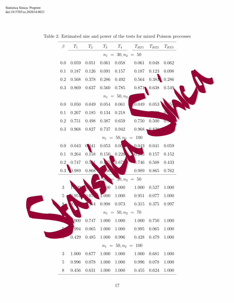
Table 2: Estimated size and power of the tests for mixed Poisson processes

β T1 T2 T3 T4 TBZ1 TBZ2 TBZ3

n1 = 30, n2 = 50

0.0 0.059 0.051 0.061 0.058 0.061 0.048 0.062

0.1 0.187 0.126 0.091 0.157 0.187 0.123 0.098

0.2 0.568 0.378 0.286 0.492 0.564 0.381 0.286

0.3 0.869 0.637 0.560 0.785 0.871 0.638 0.549

n1 = 50, n2 = 70

0.0 0.050 0.049 0.054 0.061 0.049 0.053 0.054

0.1 0.267 0.185 0.134 0.218 0.270 0.189 0.133

0.2 0.751 0.498 0.387 0.659 0.750 0.500 0.391

0.3 0.968 0.827 0.737 0.942 0.968 0.828 0.738

n1 = 50, n2 = 100

0.0 0.043 0.041 0.053 0.055 0.043 0.041 0.059

0.1 0.264 0.158 0.150 0.226 0.263 0.157 0.152

0.2 0.747 0.501 0.425 0.675 0.746 0.508 0.433

0.3 0.989 0.868 0.756 0.963 0.989 0.865 0.762

n1 = 30, n2 = 50

3 1.000 0.509 1.000 1.000 1.000 0.527 1.000

5 0.951 0.076 1.000 1.000 0.951 0.077 1.000

8 0.317 0.384 0.998 0.973 0.315 0.375 0.997

n1 = 50, n2 = 70

3 1.000 0.747 1.000 1.000 1.000 0.750 1.000

5 0.994 0.065 1.000 1.000 0.995 0.065 1.000

8 0.429 0.485 1.000 0.996 0.428 0.479 1.000

n1 = 50, n2 = 100

3 1.000 0.677 1.000 1.000 1.000 0.681 1.000

5 0.996 0.078 1.000 1.000 0.996 0.078 1.000

8 0.456 0.631 1.000 1.000 0.455 0.624 1.000

17


−3 −2 −1 0 1 2 3

−3−2

−10

12

3

Normal Q−Q Plot

Theoretical Quantiles

Sam

ple Q

uant

iles

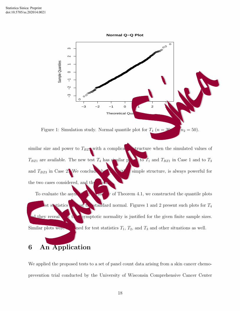
Figure 1: Simulation study. Normal quantile plot for T4 (n = 30 and n2 = 50).

similar size and power to TBZ1 with a complicated structure when the simulated values of

TBZ1 are available. The new test T4 has similar power to T1 and TBZ1 in Case 1 and to T3

and TBZ3 in Case 2. We conclude that T4, with a simple structure, is always powerful for

the two cases considered, and thus robust.

To evaluate the asymptotic normality of Theorem 4.1, we constructed the quantile plots

of the test statistics against the standard normal. Figures 1 and 2 present such plots for T4

and they reveal that the asymptotic normality is justified for the given finite sample sizes.

Similar plots were obtained for test statistics T1, T2, and T3 and other situations as well.

6 An Application

We applied the proposed tests to a set of panel count data arising from a skin cancer chemo-

prevention trial conducted by the University of Wisconsin Comprehensive Cancer Center

18


−3 −2 −1 0 1 2 3

−3−2

−10

12

3

Normal Q−Q Plot

Theoretical Quantiles

Sam

ple Q

uant

iles

Figure 2: Simulation study. Normal quantile plot for T4 (n1 = 50 and n2 = 70).

in Madison, Wisconsin. It was a double-blinded and placebo-controlled randomized phase

III clinical trial. The primary objective of this trial was to evaluate the effectiveness of

0.5g/m2/day PO difluoromethylornithine (DFMO) in reducing new skin cancers in a pop-

ulation of the patients with a history of non-melanoma skin cancers: basal cell carcinoma

and squamous cell carcinoma. The study consisted of 290 patients who were randomized to

two groups: DFMO group (143) or the placebo group (147). The observed data included a

sequence of observation times in days and the numbers of occurrences of both basal cell car-

cinoma and squamous cell carcinoma between the observation times for patients in different

treatment groups (see Table 9.3 of Sun and Zhao (2013)). Sun and Zhao (2013) analyzed

these data and found that the overall DFMO treatment seemed to have some mild effects

in reducing the recurrence rates of basal cell carcinoma and quamous cell carcinoma. In

addition, they presented a graphical comparison of the two groups and concluded that the

19


DFMO treatment seemed to have some effects in reducing the recurrence rate of basal cell

carcinoma but not to have any effect on the recurrence rate of squamous cell carcinoma. For

this reason, we focused on comparing two treatment groups in terms of the recurrence rates

of basal cell carcinoma.

To test the difference between the two groups, we treated the DFMO group as group

1 and the placebo group as group 2. Let Ni(t) represent the number of the occurrences

of basal cell carcinoma up to time t for patient i, i = 1, . . . , 290. Let Λl(t) denote the

expected occurrences of basel cell carcinoma up to time t for group l. The goal is to test

H0 : Λ1(t) = Λ2(t) = Λ0(t). The spline likelihood estimates Λl and Λ0 of Λl and Λ0 based

on samples from all the patients in the l-th group and the pooled data are shown in Figure

3. We applied the test procedure of Section 4 to this problem and obtained T1 = −2.2285,

T2 = −0.9245, T3 = −2.0245, and T4 = −2.1940 where Tj’s are as defined in Section 5,

giving p-values of 0.0258, 0.3552, 0.0429, and 0.0282 based on the standard normal. The

test results from T1, T3 and T4 suggest that the incidence rates of basal cell carcinoma were

significantly reduced by the DFMO treatment, while test T2 fails to reject H0. This can be

easily understood by looking at the behavior of the estimates. From Figure 3, the difference

of mean functions at later times dominate the difference at earlier times so that the test with

W(2)n could not detect the difference between two groups.

7 Concluding Remarks

For semiparametric models, Wellner and Zhang (2007) developed a general theorem for

deriving the asymptotic normality of semiparametric M -estimators of regression parameters.

20


0 500 1000 1500

0.0

0.5

1.0

1.5

Time (Days)

Mea

n Fu

nctio

n

DFMOPlaceboPooled

Figure 3: The estimated mean functions for the skin cancer study.

We can establish similar theory. For example, we have the following results about the

asymptotic normality of estimators in the semiparametric model considered by Wellner and

Zhang (2007) and Lu, Zhang and Huang (2009). Suppose that for each subject, given a

d-dimensional vector of covariates Zi, Ni(t) is a non-homogeneous Poisson process with the

mean function Λi(t|Zi) = Λ0(t) exp{Z ′iβ}, where Λ0 is an unknown baseline mean function

and β is a d-dimensional vector of unknown regression parameters.

Let θpsn = (βpsn , Λpsn ) and θn = (βn, Λn) be the semiparametric pseudo-likelihood and

likelihood estimators of Lu, Zhang, and Huang (2009). Let Bd denote the collection of Borel

sets in Rd, and B and B[0,τ ] as defined in Section 3. Let F be the cumulative distribution

function of Z. We considered measures ν1 and ν2 as follows: for B,B1, B2 ∈ B[0,τ ], and

21


B3 ∈ Bd,

ν1(B ×B3) =

∫B3

∞∑k=1

P (K = k|Z = z)k∑j=1

P (Tk,j ∈ B|K = k, Z = z)dF (z),

ν2(B1 ×B2 ×B3)

=

∫B3

∞∑k=1

{P (K = k|Z = z)

×k∑j=1

P (Tk,j−1 ∈ B1, Tk,j ∈ B2|K = k, Z = z)

}dF (z).

Take Hr ={

(h1, h2) : h1 ∈ Rd, ||h1|| ≤ 1, h2 ∈ Hr, h2(0) = 0}. Under some regularity con-

ditions,

(i) For (h1, h2) ∈ Hr, h′1√n(βpsn − β0) +

√n∫{Λps

n (t) − Λ0(t)}dh2(t) is asymptotically

normal.

(ii) For (h1, h2) ∈ Hr, h′1

√n(βn−β0)+

√n∫{Λn(t)−Λ0(t)}dh2(t) is asymptotically normal.

(iii) (Asymptotic Normality of βpsn )√n(βpsn −β0)→d N(0,Σps), where Σps = (Aps)−1Bps((Aps)−1))′

with

Aps = E

K∑j=1

Λ0(TK,j)eβ′0Z

{Z −

E(Zeβ

′0Z |K,TK,j

)E(eβ

′0Z |K,TK,j

) }⊗2 ,

Bps = E

[K∑j=1

K∑j′=1

{N(TK,j)− Λ0(TK,j)e

β′0Z}

×{N(TK,j′)− Λ0(TK,j′)e

β′0Z}

×

{Z −

E(Zeβ

′0Z |K,TK,j

)E(eβ

′0Z |K,TK,j

) }

×

{Z −

E(Zeβ

′0Z |K,TK,j′

)E(eβ

′0Z |K,TK,j′

) }′] ,

22


and (Asymptotic Normality of Functional of Λpsn ) for h ∈ Hr,

√n

∫{Λps

n (t)− Λ0(t)}eβ′0z

×

{h(t)

Λ0(t)− z′ (Γps)−1E

(Zeβ

′0Z

K∑j=1

h(TK,j)

)}dν1(t, z)

→d N(0, σ21),

where

Γps = E

[ZZ ′

K∑j=1

Λ0(TK,j)eβ′0Z

],

σ21 = E

[K∑j=1

{N(TK,j)− Λ0(TK,j)e

β′0Z}

×

{h(TK,j)

Λ0(TK,j)− Z ′ (Γps)−1E

(Zeβ

′0Z

K∑j′=1

h(TK,j′)

)}]2

.

(iv) (Asymptotic Normality of βn)√n(βn − β0) →d N(0,Σ), where Σ = (A)−1B((A)−1))′

with

A = E

K∑j=1

∆Λ0(TK,j)eβ′0Z

{Z −

E(Zeβ

′0Z |K,TK,j−1, TK,j

)E(eβ


) }⊗2 ,

B = E

[K∑j=1

K∑j′=1

{∆N(TK,j)−∆Λ0(TK,j)e

β′0Z}

×{

∆N(TK,j′)−∆Λ0(TK,j′)eβ′0Z}

×

{Z −

E(Zeβ


)E(eβ


) }

×

{Z −

E(Zeβ

′0Z |K,TK,j′−1, TK,j′

)E(eβ

′0Z |K,TK,j′−1, TK,j′

) }′]

and (Asymptotic Normality of Functional of Λn) for h ∈ Hr,

√n

∫ {(Λn(t)− Λn(s)

)− (Λ0(t)− Λ0(s))

}eβ

′0z

23


×

{h(t)− h(s)

Λ0(t)− Λ0(s)− z′Γ−1E

(Zeβ

′0Z

K∑j=1

∆h(TK,j)

)}dν2(s, t, z)

→d N(0, σ22),

where

Γ = E

[ZZ ′

K∑j=1

∆Λ0(TK,j)eβ′0Z

],

σ22 = E

[K∑j=1

{∆N(TK,j)−∆Λ0(TK,j)e

β′0Z}

×

{∆h(TK,j)

∆Λ0(TK,j)− Z ′Γ−1E

(Zeβ

′0Z

K∑j′=1

∆h(TK,j′)

)}]2

.

Here, the obtained asymptotic distributions for βpsn and βn are the same as those in The-

orem 3.3 of Wellner and Zhang (2007) and Theorem 3 of Lu, Zhang, and Huang (2009). The

new results about the baseline mean function can be used to conduct statistical hypothesis

tests. The proofs of the above conclusions are available from the authors.

Supplementary Materials

The supplementary materials include proofs of theorems.

Acknowledgements

The authors would like to thank the Editor, an associate editor and the two referees

for helpful comments and suggestions that greatly improved the paper. Zhao’s research was

supported in part by the Research Grant Council of Hong Kong (503513), the Natural Science

Foundation of China (11371299), and The Hong Kong Polytechnic University. Zhang’s

research was partially supported by the NSFC grant (471420107023).

24


References

Balakrishnan, N. and Zhao, X. (2009). New multi-sample nonparametric tests for panel

count data. Ann. Statist. 37, 1112–1149.

Groeneboom, P. (1996). Lectures on Inverse Problems. In Lecture Notes in Mathematics

1648, 67–164. Springer-Verlag, Berlin.

Groeneboom, P. and Wellner, J. A. (1992). Information Bounds and Nonparametric Max-

imum Likelihood Estimation. Birkhauser, New York.

Hu X. J., Lagakos, S. W., and Lockhart, R. A. (2009a). Marginal analysis of panel counts

through estimating functions. Biometrika 96, 445–456.

Hu, X. J., Lagakos, S. W., and Lockhart, R. A. (2009b). Generalized least squares estima-

tion of the mean function of a counting process based on panel counts. Statist. Sinica

19, 561–580.

Lu, M., Zhang, Y., and Huang, J. (2007). Estimation of the mean function with panel

count data using monotone polynomial splines. Biometrika 94, 705–718.

Lu, M., Zhang, Y., and Huang, J. (2009). Semiparametric estimation methods for panel

count data using monotone B-splines. J. Amer. Statist. Assoc. 104, 1060–1070.

Schick, A. and Yu, Q. (2000). Consistency of the GMLE with mixed case interval-censored

data. Scand. J. Statist. 27, 45–55.

Schumaker, L. (1981). Spline Functions: Basic Theory. Wiley: New York. .

25


Shen, X. and Wong, W. H. (1994). Convergence rate of sieve estimates. Ann. Statist. 18,

580–615.

Sun, J. and Fang, H. B. (2003). A nonparametric test for panel count data. Biometrika

90, 199–208.

Sun, J. and Kalbfleisch, J. D. (1995). Estimation of the mean function of point processes

based on panel count data. Statist. Sinica 5, 279–290.

Sun, J. and Zhao, X. (2013). Statistical Analysis of Panel Count Data. Springer, New

York.

Thall, P. F. and Lachin, J. M. (1988). Analysis of recurrent events: nonparametric methods

for random-interval count data. J. Amer. Statist. Assoc. 83, 339–347.

van der Vaart, A. W. and Wellner, J. A. (1996). Weak Convergence and Empirical Pro-

cesses. Springer-Verlag: New York.

Wellner, J. A. and Zhang, Y. (2000). Two estimators of the mean of a counting process

with panel count data. Ann. Statist. 28, 779–814.

Wellner, J. A. and Zhang, Y. (2007). Two likelihood-based semiparametric estimation

methods for panel count data with covariates. Ann. Statist. 35, 2106–2142.

Zeng, D. and Lin, D. Y. (2006). Efficient estimation of semiparametric transformation

models for counting processes. Biometrika 93, 627–640.

Zeng, D. and Lin, D. Y. (2007). Semiparametric transformation models with random effects

for recurrent events. J. Amer. Statist. Assoc. 102, 1387–1396.

26


Zeng, D., Lin, D. Y., and Yin, G. S. (2005). Maximum likelihood estimation for the

proportional odds model with random effects. J. Amer. Statist. Assoc. 100, 470–482.

Zhang, Y. (2006). Nonparametric k-sample tests for panel count data. Biometrika 93,

777–790.

Department of Applied Mathematics, The Hong Kong Polytechnic University, Hong Kong,

China and The Hong Kong Polytechnic University Shenzhen Research Institute, China.

E-mail: [email protected]

Department of Biostatistics, Indiana University, Indianapolis, IN 46202, USA.

E-mail: [email protected]

27


m-estimators with applications to hypothesis testing for

Documents