lyapunov and invariance methods in control design · logo lyapunov and invariance methods in...
TRANSCRIPT

logo
Lyapunov and invariance methods in control design
Franco Blanchini 1
1Dipartimento di Matematica e InformaticaUniversita degli Studi di Udine
IFAC Joint conference, Grenoble, February 4, 2013
F. Blanchini Lyapunov and invariance methods in control design

logo
General
The purposes of the talk are
F. Blanchini Lyapunov and invariance methods in control design

logo
General
The purposes of the talk are
Overview of set theoretic concepts;
F. Blanchini Lyapunov and invariance methods in control design

logo
General
The purposes of the talk are
Overview of set theoretic concepts;
Invariance and Lyapunov techniques;
F. Blanchini Lyapunov and invariance methods in control design

logo
General
The purposes of the talk are
Overview of set theoretic concepts;
Invariance and Lyapunov techniques;
Ideas and applications.
F. Blanchini Lyapunov and invariance methods in control design

logo
Dynamic Programming 1
A general problem
x(t+1) = f (x(t),u(t),w(t))
F. Blanchini Lyapunov and invariance methods in control design

logo
Dynamic Programming 1
A general problem
x(t+1) = f (x(t),u(t),w(t))
Constraints:
- On the disturbance w(t) ∈ W ;- On the control input u(t) ∈ U ;- On the state x(t) ∈ X ;
F. Blanchini Lyapunov and invariance methods in control design

logo
Dynamic Programming 1
A general problem
x(t+1) = f (x(t),u(t),w(t))
Constraints:
- On the disturbance w(t) ∈ W ;- On the control input u(t) ∈ U ;- On the state x(t) ∈ X ;
Problem–State in a tube: Find a control u =Φ(x) andXini ⊆ X such that and for all x(0) ∈ Xini and w(t) ∈ W
x(t) ∈ X , t ≥ 0,
u(t) ∈ U , t ≥ 0.
F. Blanchini Lyapunov and invariance methods in control design
logo
Dynamic Programming 2
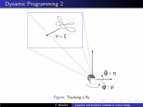
v
ρ
ζ
θ
φ
η
Figure: Tracking a fly
F. Blanchini Lyapunov and invariance methods in control design

logo
Dynamic Programming 3
r
Figure: Tracking a fly
F. Blanchini Lyapunov and invariance methods in control design

logo
Dynamic Programming 3
horizontal
vert
ical
r
Figure: Tracking a fly
F. Blanchini Lyapunov and invariance methods in control design
logo
Dynamic Programming 4
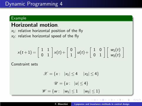
Example
Horizontal motion.x1: relative horizontal position of the flyx2: relative horizontal speed of the fly
x(t+1) =
[
1 10 1
]
x(t)+
[
01
]
u(t)+
[
1 00 1
][
w1(t)w2(t)
]
Constraint sets
X = x : |x1| ≤ 4 |x2| ≤ 4
U = u : |u| ≤ 4
W = w : |w1| ≤ 1 |w2| ≤ 1
F. Blanchini Lyapunov and invariance methods in control design

logo
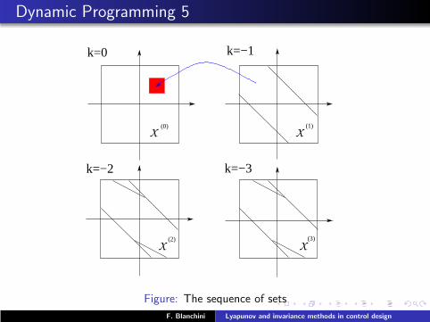
Dynamic Programming 5
k=0
X(0)
Figure: The sequence of sets
F. Blanchini Lyapunov and invariance methods in control design

logo
Dynamic Programming 5
k=0 k=−1
X X(1)(0)
Figure: The sequence of sets
F. Blanchini Lyapunov and invariance methods in control design

logo
Dynamic Programming 5
k=0 k=−1
k=−2
X X
X(2)
(1)(0)
Figure: The sequence of sets
F. Blanchini Lyapunov and invariance methods in control design
logo
Dynamic Programming 5
k=0 k=−1
k=−2 k=−3
X X
X(2)
(1)(0)
(3)
X
Figure: The sequence of sets
F. Blanchini Lyapunov and invariance methods in control design
logo
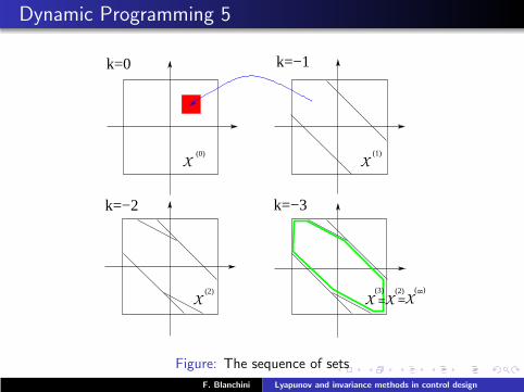
Dynamic Programming 5
k=0 k=−1
k=−2 k=−3
X X
X(2)
(1)(0)
(3)
X =X(2)=X
8( )
Figure: The sequence of sets
F. Blanchini Lyapunov and invariance methods in control design

logo
Dynamic Programming 6
One–step controllability set to S
C (S ) = x : ∃u ∈ U : x+ = f (x ,u,w) ∈ S , ∀w ∈ W
F. Blanchini Lyapunov and invariance methods in control design

logo
Dynamic Programming 6
One–step controllability set to S
C (S ) = x : ∃u ∈ U : x+ = f (x ,u,w) ∈ S , ∀w ∈ W
Procedure
F. Blanchini Lyapunov and invariance methods in control design

logo
Dynamic Programming 6
One–step controllability set to S
C (S ) = x : ∃u ∈ U : x+ = f (x ,u,w) ∈ S , ∀w ∈ W
Procedure
1 Define X0 = X ;
F. Blanchini Lyapunov and invariance methods in control design

logo
Dynamic Programming 6
One–step controllability set to S
C (S ) = x : ∃u ∈ U : x+ = f (x ,u,w) ∈ S , ∀w ∈ W
Procedure
1 Define X0 = X ;
2 Define recursively backward in time
X(k−1) = C (X (k))
⋂
X
F. Blanchini Lyapunov and invariance methods in control design

logo
Dynamic Programming 6
One–step controllability set to S
C (S ) = x : ∃u ∈ U : x+ = f (x ,u,w) ∈ S , ∀w ∈ W
Procedure
1 Define X0 = X ;
2 Define recursively backward in time
X(k−1) = C (X (k))
⋂
X
3 DefineXmax =
⋂
k≤0
X(k)
F. Blanchini Lyapunov and invariance methods in control design

logo
Dynamic Programming 7
Theorem
Assume that U , X and W are compact. The problem of keepingthe state in a tube has a solution iff
Xmax 6= /0
Xmax : set of all initial states for which the problem has a solution.
F. Blanchini Lyapunov and invariance methods in control design

logo
Dynamic Programming 7
Theorem
Assume that U , X and W are compact. The problem of keepingthe state in a tube has a solution iff
Xmax 6= /0
Xmax : set of all initial states for which the problem has a solution.
Control:
u =Φ(x) ∈ Ω(x) = u ∈ U : f (x ,u,w) ∈ Xmax , ∀w ∈ W
x ∈ Xmax ⇔ Ω(x) 6= /0.
Bertsekas and Rhodes – Glower and Scheppe (1972)
F. Blanchini Lyapunov and invariance methods in control design

logo
Dynamic Programming 8
Related problems
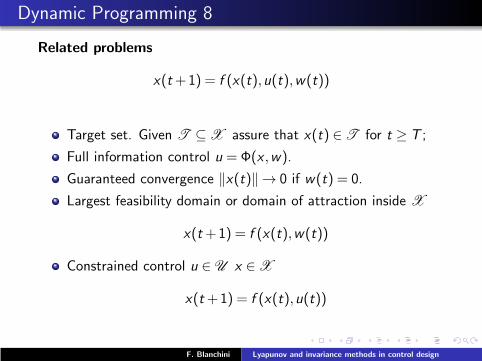
x(t+1) = f (x(t),u(t),w(t))
F. Blanchini Lyapunov and invariance methods in control design

logo
Dynamic Programming 8
Related problems
x(t+1) = f (x(t),u(t),w(t))
Target set. Given T ⊆ X assure that x(t) ∈ T for t ≥ T ;
F. Blanchini Lyapunov and invariance methods in control design

logo
Dynamic Programming 8
Related problems
x(t+1) = f (x(t),u(t),w(t))
Target set. Given T ⊆ X assure that x(t) ∈ T for t ≥ T ;
Full information control u =Φ(x ,w).
F. Blanchini Lyapunov and invariance methods in control design

logo
Dynamic Programming 8
Related problems
x(t+1) = f (x(t),u(t),w(t))
Target set. Given T ⊆ X assure that x(t) ∈ T for t ≥ T ;
Full information control u =Φ(x ,w).
Guaranteed convergence ‖x(t)‖→ 0 if w(t) = 0.
F. Blanchini Lyapunov and invariance methods in control design

logo
Dynamic Programming 8
Related problems
x(t+1) = f (x(t),u(t),w(t))
Target set. Given T ⊆ X assure that x(t) ∈ T for t ≥ T ;
Full information control u =Φ(x ,w).
Guaranteed convergence ‖x(t)‖→ 0 if w(t) = 0.
Largest feasibility domain or domain of attraction inside X
x(t+1) = f (x(t),w(t))
F. Blanchini Lyapunov and invariance methods in control design
logo
Dynamic Programming 8
Related problems
x(t+1) = f (x(t),u(t),w(t))
Target set. Given T ⊆ X assure that x(t) ∈ T for t ≥ T ;
Full information control u =Φ(x ,w).
Guaranteed convergence ‖x(t)‖→ 0 if w(t) = 0.
Largest feasibility domain or domain of attraction inside X
x(t+1) = f (x(t),w(t))
Constrained control u ∈ U x ∈ X
x(t+1) = f (x(t),u(t))
F. Blanchini Lyapunov and invariance methods in control design

logo
Dynamic Programming 9
F. Blanchini Lyapunov and invariance methods in control design

logo
Dynamic Programming 9
Claim
First message: 40 years ago we had the basic theory to deal withthe “state in a tube problem”.
F. Blanchini Lyapunov and invariance methods in control design

logo
Positive invariance 1
F. Blanchini Lyapunov and invariance methods in control design

logo
Positive invariance 1
Definition
The set P is (robustly) positively invariant for the system
x(t+1) = f (x(t),w(t))
if x(τ ) ∈ P implies x(t) ∈ P for t ≥ τ .
F. Blanchini Lyapunov and invariance methods in control design

logo
Positive invariance 1
Definition
The set P is (robustly) positively invariant for the system
x(t+1) = f (x(t),w(t))
if x(τ ) ∈ P implies x(t) ∈ P for t ≥ τ .
Definition
The set P is (robustly) controlled invariant for the system
x(t+1) = f (x(t),u(t),w(t))
if there exists a control law u =Φ(x) ∈ U such that P ispositively invariant for
x(t+1) = f (x(t),w(t),Φ(x(t)))
F. Blanchini Lyapunov and invariance methods in control design

logo
Positive invariance 2
F. Blanchini Lyapunov and invariance methods in control design
logo
Positive invariance 2
Theorem
The “state in a tube” problem has a solution iff there exists acontrolled–invariant set
P ⊆ X
F. Blanchini Lyapunov and invariance methods in control design

logo
Positive invariance 2
Theorem
The “state in a tube” problem has a solution iff there exists acontrolled–invariant set
P ⊆ X
The set Xmax is the maximal–controlled invariant set.
F. Blanchini Lyapunov and invariance methods in control design

logo
Positive invariance 2
Theorem
The “state in a tube” problem has a solution iff there exists acontrolled–invariant set
P ⊆ X
The set Xmax is the maximal–controlled invariant set.
In practice we might be satisfied with some P smaller butsimpler
F. Blanchini Lyapunov and invariance methods in control design
logo
Positive invariance 3
Problem
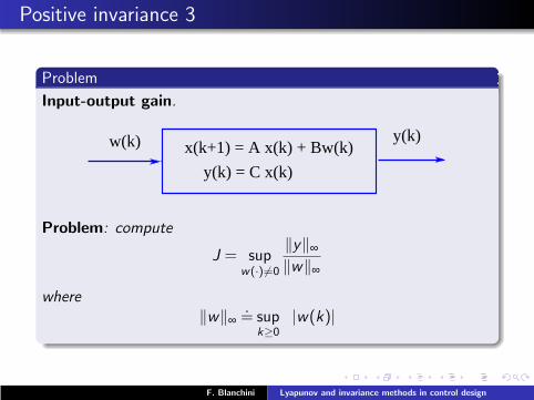
Input-output gain.
w(k) y(k)x(k+1) = A x(k) + Bw(k)
y(k) = C x(k)
Problem: compute
J = supw(·) 6=0
‖y‖∞
‖w‖∞
where‖w‖∞
.= sup
k≥0|w(k)|
F. Blanchini Lyapunov and invariance methods in control design

logo
Positive invariance 4
F. Blanchini Lyapunov and invariance methods in control design

logo
Positive invariance 4
The question is not well–posed since x(0) is not specified.
F. Blanchini Lyapunov and invariance methods in control design
logo
Positive invariance 4
The question is not well–posed since x(0) is not specified.
If x(0) = 0, thenJ = ∑
k≥0
|CAkB |.
F. Blanchini Lyapunov and invariance methods in control design

logo
Positive invariance 4
The question is not well–posed since x(0) is not specified.
If x(0) = 0, thenJ = ∑
k≥0
|CAkB |.
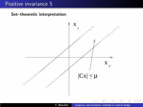
Set theoretic condition
Proposition
J ≤ µ iff there exists a positively invariant set P such that
P ⊂ x : |Cx | ≤ µ
F. Blanchini Lyapunov and invariance methods in control design

logo
Positive invariance 5
Set–theoretic interpretation:
2x
1x
F. Blanchini Lyapunov and invariance methods in control design
logo
Positive invariance 5
Set–theoretic interpretation:
2x
1x
|Cx| <µ
F. Blanchini Lyapunov and invariance methods in control design

logo
Positive invariance 5
Set–theoretic interpretation:
2x
1x
|Cx| <µP
F. Blanchini Lyapunov and invariance methods in control design

logo
Positive invariance 6
x
x
P
µ
1
2
g(x) <
x =f(x,w) +
Figure: Advantages: Set–theoretic works for nonlinearF. Blanchini Lyapunov and invariance methods in control design

logo
Positive invariance 7
F. Blanchini Lyapunov and invariance methods in control design
logo
Positive invariance 7
The condition |y | ≤ µ is satisfied for all x(0) ∈ P.
F. Blanchini Lyapunov and invariance methods in control design

logo
Positive invariance 7
The condition |y | ≤ µ is satisfied for all x(0) ∈ P.
The set theoretic conditions works for uncertain and nonlinearsystems.
F. Blanchini Lyapunov and invariance methods in control design

logo
Positive invariance 7
The condition |y | ≤ µ is satisfied for all x(0) ∈ P.
The set theoretic conditions works for uncertain and nonlinearsystems.
Synthesis case: potential advantages of nonlinear controllers
F. Blanchini Lyapunov and invariance methods in control design

logo
Invariant sets and Lyapunov functions 1
x(t) = f (x(t)), 0 = f (0)
orx(t+1) = f (x(t))
F. Blanchini Lyapunov and invariance methods in control design

logo
Invariant sets and Lyapunov functions 1
x(t) = f (x(t)), 0 = f (0)
orx(t+1) = f (x(t))
Definition
A Lyapunov function is a positive–definite function which isdecreasing (non–increasing) along the system trajectories:
V (x(t2))< V (x(t1)), if t1 ≤ t2
Typically: V (x) = ∇ V (x)f (x)< 0 or ∆V (x)< 0.
F. Blanchini Lyapunov and invariance methods in control design

logo
Invariant sets and Lyapunov functions 2
Controlled systems:
x(t) = f (x(t),u(t)), 0 = f (0,0)
or
x(k+1) = f (x(k),u(k)),
F. Blanchini Lyapunov and invariance methods in control design

logo
Invariant sets and Lyapunov functions 2
Controlled systems:
x(t) = f (x(t),u(t)), 0 = f (0,0)
or
x(k+1) = f (x(k),u(k)),
Definition
A Control Lyapunov function is a positive–definite function whichbecomes a Lyapunov function if a proper feedback u = κ (x) isapplied:
x(t) = f (x(t),κ (x(t))),
F. Blanchini Lyapunov and invariance methods in control design

logo
Invariant sets and Lyapunov functions 3
Fact
The sub-level set
N [V ,κ ] .= x : V (x)≤ κ
are positively invariant.
F. Blanchini Lyapunov and invariance methods in control design

logo
Invariant sets and Lyapunov functions 3
Fact
The sub-level set
N [V ,κ ] .= x : V (x)≤ κ
are positively invariant.
Any LF generates invariant sets.
F. Blanchini Lyapunov and invariance methods in control design

logo
Invariant sets and Lyapunov functions 3
Fact
The sub-level set
N [V ,κ ] .= x : V (x)≤ κ
are positively invariant.
Any LF generates invariant sets.
Given an invariant set, there is no obvious way to associate aLF with it.
F. Blanchini Lyapunov and invariance methods in control design

logo
Invariant sets and Lyapunov functions 3
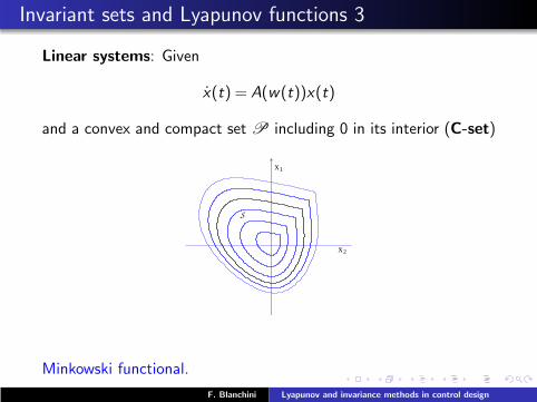
Linear systems: Given
x(t) = A(w(t))x(t)
and a convex and compact set P including 0 in its interior (C-set)
S
x
x2
1
Minkowski functional.
F. Blanchini Lyapunov and invariance methods in control design
logo
Invariant sets and Lyapunov functions 3
Linear systems: Given
x(t) = A(w(t))x(t)
and a convex and compact set P including 0 in its interior (C-set)
S
x
x2
1
Minkowski functional.
F. Blanchini Lyapunov and invariance methods in control design

logo
Controlled invariance of ellipsoids
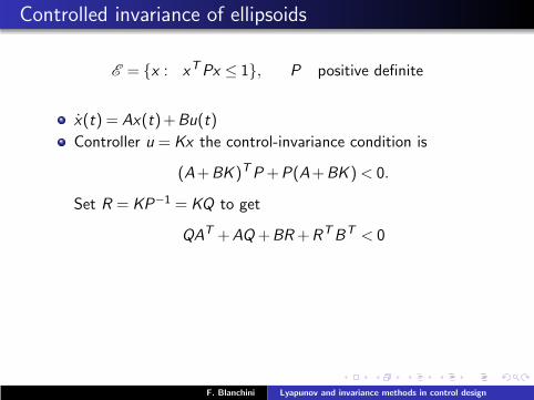
E = x : xTPx ≤ 1, P positive definite
F. Blanchini Lyapunov and invariance methods in control design

logo
Controlled invariance of ellipsoids
E = x : xTPx ≤ 1, P positive definite
x(t) = Ax(t)+Bu(t)
F. Blanchini Lyapunov and invariance methods in control design
logo
Controlled invariance of ellipsoids
E = x : xTPx ≤ 1, P positive definite
x(t) = Ax(t)+Bu(t)
Controller u = Kx the control-invariance condition is
(A+BK )TP+P(A+BK )< 0.
Set R = KP−1 = KQ to get
QAT +AQ+BR+RTBT < 0
F. Blanchini Lyapunov and invariance methods in control design
logo
Controlled invariance of ellipsoids
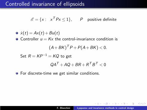
E = x : xTPx ≤ 1, P positive definite
x(t) = Ax(t)+Bu(t)
Controller u = Kx the control-invariance condition is
(A+BK )TP+P(A+BK )< 0.
Set R = KP−1 = KQ to get
QAT +AQ+BR+RTBT < 0
For discrete-time we get similar conditions.
F. Blanchini Lyapunov and invariance methods in control design

logo
Controlled invariance of ellipsoids
E = x : xTPx ≤ 1, P positive definite
x(t) = Ax(t)+Bu(t)
Controller u = Kx the control-invariance condition is
(A+BK )TP+P(A+BK )< 0.
Set R = KP−1 = KQ to get
QAT +AQ+BR+RTBT < 0
For discrete-time we get similar conditions.
Claim
(Almost) nothing is forgotten in the LMI world: disturbance,constraints, performances, delays, uncertainties, LPV, disturbancerejection ... Boyd, El Ghaoui, Feron, Balakrishnan
F. Blanchini Lyapunov and invariance methods in control design

logo
Competitors?
F. Blanchini Lyapunov and invariance methods in control design

logo
Competitors?
Question
Are there other convenient classes of Lyapunov functions?
F. Blanchini Lyapunov and invariance methods in control design

logo
Competitors: polyhedral Lyapunov functions
V (x) = maxi
Fix∑ pi : pi PERLOSPAZIO
F. Blanchini Lyapunov and invariance methods in control design

logo
Competitors: polyhedral Lyapunov functions
V (x) = min∑ pi : pi ≥ 0, x = Xp
F. Blanchini Lyapunov and invariance methods in control design
logo
Controlled invariance of polyhedra 1
Consider the set
P = x = Xp, p ≥ 0, ∑pi = 1
and x(t) = Ax(t)+Bu(t). Controlled invariance requires
Pij ≥ 0, i 6= j
AX +BU = XP
1TP ≤ −β 1T , β ≥ 0
where 1T = [ 1 1 . . . 1 ].
Non–linear unless x is fixed.
But we can use backward–recursive procedures.
F. Blanchini Lyapunov and invariance methods in control design

logo
Controlled invariance of polyhedra 1
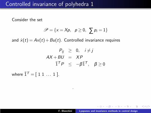
Consider the set
P = x = Xp, p ≥ 0, ∑pi = 1
and x(t) = Ax(t)+Bu(t). Controlled invariance requires
Pij ≥ 0, i 6= j
AX +BU = XP
1TP ≤ −β 1T , β ≥ 0
where 1T = [ 1 1 . . . 1 ].
Non–linear unless X is fixed....
... but we can use backward–recursive procedures.
F. Blanchini Lyapunov and invariance methods in control design

logo
Controlled invariance of polyhedra 1
Consider the set
P = x = Xp, p ≥ 0, ∑pi = 1
and x(t) = Ax(t)+Bu(t). Controlled invariance requires
Pij ≥ 0, i 6= j
AX +BU = XP
1TP ≤ −β 1T , β ≥ 0
where 1T = [ 1 1 . . . 1 ].
Non–linear unless X is fixed....
...but we can use backward–recursive procedures.
F. Blanchini Lyapunov and invariance methods in control design

logo
Controlled invariance of polyhedra 2
In general a controlled–invariant polyhedron does not admit linearcontrollers, but a piecewise–linear control.
Gutman and Cwikel (1986)... yes ... but how many sectors are needed?
F. Blanchini Lyapunov and invariance methods in control design

logo
Controlled invariance of polyhedra 3
In general a controlled–invariant polyhedron does not admit linearcontrollers, but a piecewise–linear control.
u = K x
h
Gutman and Cwikel (1986)... yes ... but how many sectors are needed?
F. Blanchini Lyapunov and invariance methods in control design
logo
Controlled invariance of polyhedra 3
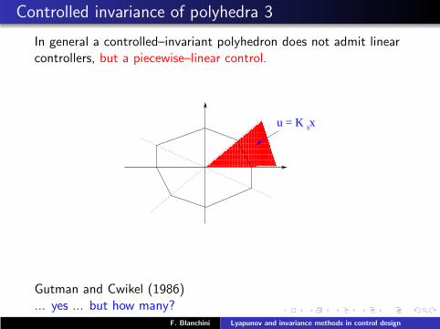
In general a controlled–invariant polyhedron does not admit linearcontrollers, but a piecewise–linear control.
u = K x
h
Gutman and Cwikel (1986)... yes ... but how many?
F. Blanchini Lyapunov and invariance methods in control design
logo
Controlled invariance of polyhedra 4
F. Blanchini Lyapunov and invariance methods in control design

logo
Controlled invariance of polyhedra
-1.0 -0.8 -0.6 -0.4 -0.2 0.0 0.2 0.4 0.6 0.8 1.0
-1.0
-0.8
-0.6
-0.4
-0.2
0.0
0.2
0.4
0.6
0.8
1.0
-1.0 -0.8 -0.6 -0.4 -0.2 0.0 0.2 0.4 0.6 0.8 1.0
-1.0
-0.8
-0.6
-0.4
-0.2
0.0
0.2
0.4
0.6
0.8
1.0
1
234
567
89
10
Controlled–invariant with constraints|h1− h1| ≤ 0.1m |h2− h2| ≤ 0.1m, |u− u| ≤ 0.05m/s.
F. Blanchini Lyapunov and invariance methods in control design

logo
Controlled invariance of polyhedra 5
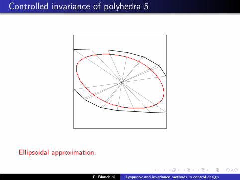
Ellipsoidal approximation.
F. Blanchini Lyapunov and invariance methods in control design
logo
Controlled invariance of polyhedra 5
Ellipsoidal approximation.
F. Blanchini Lyapunov and invariance methods in control design

logo
Limits and advantages of quadratic sets/functions
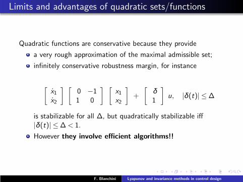
Quadratic functions are conservative because they provide
F. Blanchini Lyapunov and invariance methods in control design

logo
Limits and advantages of quadratic sets/functions
Quadratic functions are conservative because they provide
a very rough approximation of the maximal admissible set;
F. Blanchini Lyapunov and invariance methods in control design

logo
Limits and advantages of quadratic sets/functions
Quadratic functions are conservative because they provide
a very rough approximation of the maximal admissible set;
infinitely conservative robustness margin, for instance
F. Blanchini Lyapunov and invariance methods in control design

logo
Limits and advantages of quadratic sets/functions
Quadratic functions are conservative because they provide
a very rough approximation of the maximal admissible set;
infinitely conservative robustness margin, for instance
[
x1x2
] [
0 −11 0
] [
x1x2
]
+
[
δ1
]
u, |δ(t)| ≤∆
is stabilizable for all ∆, but quadratically stabilizable iff|δ(t)| ≤∆< 1.
F. Blanchini Lyapunov and invariance methods in control design
logo
Limits and advantages of quadratic sets/functions
Quadratic functions are conservative because they provide
a very rough approximation of the maximal admissible set;
infinitely conservative robustness margin, for instance
[
x1x2
] [
0 −11 0
] [
x1x2
]
+
[
δ1
]
u, |δ(t)| ≤∆
is stabilizable for all ∆, but quadratically stabilizable iff|δ(t)| ≤∆< 1.
However they involve efficient algorithms!!
F. Blanchini Lyapunov and invariance methods in control design
logo
Limits and advantages of polyhedral sets/functions
Polyhedral functions are computationally demanding because
F. Blanchini Lyapunov and invariance methods in control design
logo
Limits and advantages of polyhedral sets/functions
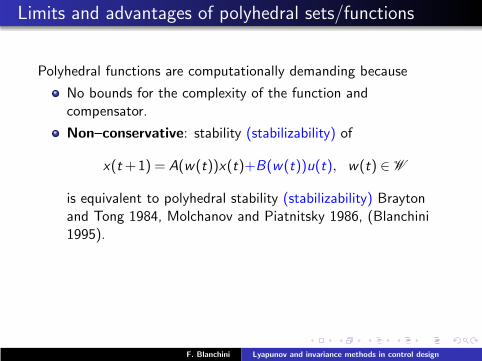
Polyhedral functions are computationally demanding because
No bounds for the complexity of the function andcompensator.
F. Blanchini Lyapunov and invariance methods in control design
logo
Limits and advantages of polyhedral sets/functions
Polyhedral functions are computationally demanding because
No bounds for the complexity of the function andcompensator.
Non–conservative: stability (stabilizability) of
x(t+1) = A(w(t))x(t)+B(w(t))u(t), w(t) ∈ W
is equivalent to polyhedral stability (stabilizability) Braytonand Tong 1984, Molchanov and Piatnitsky 1986, (Blanchini1995).
F. Blanchini Lyapunov and invariance methods in control design

logo
Limits and advantages of polyhedral sets/functions
Polyhedral functions are computationally demanding because
No bounds for the complexity of the function andcompensator.
Non–conservative: stability (stabilizability) of
x(t+1) = A(w(t))x(t)+B(w(t))u(t), w(t) ∈ W
is equivalent to polyhedral stability (stabilizability) Braytonand Tong 1984, Molchanov and Piatnitsky 1986, (Blanchini1995).
ε–approximation of the maximal controlled-invariant setMorris and Brown 1975, Gutman and Cwickel 1986, Kheertiand Gilbert 1987, (Blanchini Miani 1996).
F. Blanchini Lyapunov and invariance methods in control design

logo
Other functions
F. Blanchini Lyapunov and invariance methods in control design

logo
Other functions
Piecewise quadratic.
F. Blanchini Lyapunov and invariance methods in control design

logo
Other functions
Piecewise quadratic.
Polynomials.
F. Blanchini Lyapunov and invariance methods in control design

logo
Other functions
Piecewise quadratic.
Polynomials.
Truncated quadratic.
F. Blanchini Lyapunov and invariance methods in control design

logo
Other functions
Piecewise quadratic.
Polynomials.
Truncated quadratic.
Composite quadratic.
F. Blanchini Lyapunov and invariance methods in control design

logo
Applications
Topics which successfully involve set–invariance techniques include
F. Blanchini Lyapunov and invariance methods in control design

logo
Applications
Topics which successfully involve set–invariance techniques include
Constrained control with disturbances
F. Blanchini Lyapunov and invariance methods in control design

logo
Applications
Topics which successfully involve set–invariance techniques include
Constrained control with disturbances
Reference management
F. Blanchini Lyapunov and invariance methods in control design

logo
Applications
Topics which successfully involve set–invariance techniques include
Constrained control with disturbances
Reference management
Receding horizon control
F. Blanchini Lyapunov and invariance methods in control design

logo
Applications
Topics which successfully involve set–invariance techniques include
Constrained control with disturbances
Reference management
Receding horizon control
Switching among compensators
F. Blanchini Lyapunov and invariance methods in control design

logo
Applications
Topics which successfully involve set–invariance techniques include
Constrained control with disturbances
Reference management
Receding horizon control
Switching among compensators
Obstacle avoidance
F. Blanchini Lyapunov and invariance methods in control design
logo
Applications
Topics which successfully involve set–invariance techniques include
Constrained control with disturbances
Reference management
Receding horizon control
Switching among compensators
Obstacle avoidance
. . .
F. Blanchini Lyapunov and invariance methods in control design
logo
Control with constraints and disturbances
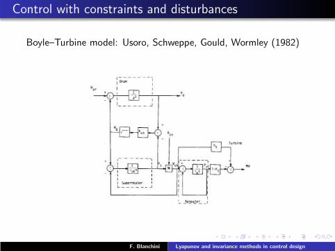
Boyle–Turbine model: Usoro, Schweppe, Gould, Wormley (1982)
F. Blanchini Lyapunov and invariance methods in control design

logo
Control with constraints and disturbances
Example
x1x2x3
=
−0.0075 −0.0075 00.1086 −0.149 0
0 0.1415 −0.1887
x1x2x3
+
0−0.05380.1187
w +
0.003700
u
|x1| ≤ 0.1, |x2| ≤ 0.01, |x3| ≤ 0.1, |u| ≤ 0.25
Maximize the disturbance size α : |w | ≤ α
F. Blanchini Lyapunov and invariance methods in control design

logo
Control with constraints and disturbances
F. Blanchini Lyapunov and invariance methods in control design
logo
Control with constraints and disturbances
Quadratic L. F. performance: αQUAD = 1.27
F. Blanchini Lyapunov and invariance methods in control design

logo
Control with constraints and disturbances
Quadratic L. F. performance: αQUAD = 1.27
Quadratic L. F. control: u =−37.85x1−4.639x2+0.475x3
F. Blanchini Lyapunov and invariance methods in control design

logo
Control with constraints and disturbances
Quadratic L. F. performance: αQUAD = 1.27
Quadratic L. F. control: u =−37.85x1−4.639x2+0.475x3
Polyhedral L. F. performance αPOLY = 1.45
F. Blanchini Lyapunov and invariance methods in control design

logo
Control with constraints and disturbances
Quadratic L. F. performance: αQUAD = 1.27
Quadratic L. F. control: u =−37.85x1−4.639x2+0.475x3
Polyhedral L. F. performance αPOLY = 1.45
Polyhedral L. F. control: Number of sectors (and gains)ns = 60.
Trade–off: if you use the linear one, you loose about 12%
F. Blanchini Lyapunov and invariance methods in control design

logo
Life is a trade–off
Claim
F. Blanchini Lyapunov and invariance methods in control design

logo
Life is a trade–off
Claim
There is almost always a trade–off between the optimalsolution which is complex or unrealistic and simpler butsub–optimal solutions.
F. Blanchini Lyapunov and invariance methods in control design
logo
Life is a trade–off
Claim
There is almost always a trade–off between the optimalsolution which is complex or unrealistic and simpler butsub–optimal solutions.
Optimal solutions support the sub–optimal ones, because ...
F. Blanchini Lyapunov and invariance methods in control design

logo
Life is a trade–off
Claim
There is almost always a trade–off between the optimalsolution which is complex or unrealistic and simpler butsub–optimal solutions.
Optimal solutions support the sub–optimal ones, because ...
... once you know the optimal you are aware of how much youare loosing when you use the sub–optimal one (Boyd–Barratt).
F. Blanchini Lyapunov and invariance methods in control design

logo
Reference management 1
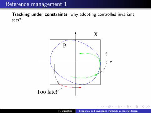
Tracking under constraints: why adopting controlled invariantsets?
X
F. Blanchini Lyapunov and invariance methods in control design

logo
Reference management 1
Tracking under constraints: why adopting controlled invariantsets?
X
Too late!
F. Blanchini Lyapunov and invariance methods in control design
logo
Reference management 1
Tracking under constraints: why adopting controlled invariantsets?
X
P
Too late!
F. Blanchini Lyapunov and invariance methods in control design

logo
Reference management 2
ReferenceRegulator PLANT
r e y+
−manager
m
Figure: Open loop Reference Management Device
F. Blanchini Lyapunov and invariance methods in control design

logo
Reference management 3
ReferenceRegulator PLANT
r e y+
−manager
m
Figure: Closed loop Reference Management Device
F. Blanchini Lyapunov and invariance methods in control design

logo
Reference management 4
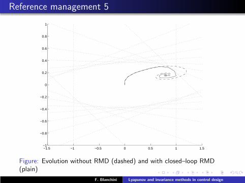
Kapasouris, Athans and Stain (1988); Tan and Gilbert (1991);Gilbert, Kolmanowski and Tan (1995); Bemporad, Casavola andMosca (1996)...
Example
1z − a
kz − 1
r
Manager
Referencey
u
m
−+
Let a= 0.8 and k = 0.08, assume x(0) = 0 let r(t)≡ 0.8.Constraint: |y | ≤ 1.
F. Blanchini Lyapunov and invariance methods in control design
logo
Reference management 5
−1.5 −1 −0.5 0 0.5 1 1.5−1
−0.8
−0.6
−0.4
−0.2
0
0.2
0.4
0.6
0.8
1
Figure: Evolution without RMD (dashed) and with closed–loop RMD(plain)
F. Blanchini Lyapunov and invariance methods in control design

logo
Reference management 6
0 10 20 30 40 50 60 70 800
0.2
0.4
0.6
0.8
1
1.2
1.4
Figure: Time evolution without RMD (dashed), with open–loop RMD(dash–dotted) and with closed loop RMD (plain)
F. Blanchini Lyapunov and invariance methods in control design

logo
Advantage of nonlinear controllers
Claim
F. Blanchini Lyapunov and invariance methods in control design

logo
Advantage of nonlinear controllers
Claim
Control performance can considerably benefit fromnon-linearities.
F. Blanchini Lyapunov and invariance methods in control design

logo
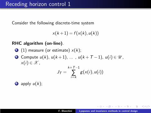
Receding horizon control 1
Consider the following discrete-time system
x(k+1) = f (x(k),u(k))
RHC algorithm (on-line).
F. Blanchini Lyapunov and invariance methods in control design
logo
Receding horizon control 1
Consider the following discrete-time system
x(k+1) = f (x(k),u(k))
RHC algorithm (on-line).
1 (1) measure (or estimate) x(k);
F. Blanchini Lyapunov and invariance methods in control design

logo
Receding horizon control 1
Consider the following discrete-time system
x(k+1) = f (x(k),u(k))
RHC algorithm (on-line).
1 (1) measure (or estimate) x(k);
2 Compute u(k), u(k+1), ... , u(k+T −1), u(i) ∈ U ,x(i) ∈ X ,
JT =k+T−1
∑i=k
g(x(i),u(i))
F. Blanchini Lyapunov and invariance methods in control design
logo
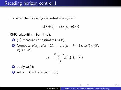
Receding horizon control 1
Consider the following discrete-time system
x(k+1) = f (x(k),u(k))
RHC algorithm (on-line).
1 (1) measure (or estimate) x(k);
2 Compute u(k), u(k+1), ... , u(k+T −1), u(i) ∈ U ,x(i) ∈ X ,
JT =k+T−1
∑i=k
g(x(i),u(i))
3 apply u(k);
F. Blanchini Lyapunov and invariance methods in control design
logo
Receding horizon control 1
Consider the following discrete-time system
x(k+1) = f (x(k),u(k))
RHC algorithm (on-line).
1 (1) measure (or estimate) x(k);
2 Compute u(k), u(k+1), ... , u(k+T −1), u(i) ∈ U ,x(i) ∈ X ,
JT =k+T−1
∑i=k
g(x(i),u(i))
3 apply u(k);
4 set k = k+1 and go to (1)
F. Blanchini Lyapunov and invariance methods in control design

logo
Receding horizon control 2
The following problems arise
F. Blanchini Lyapunov and invariance methods in control design

logo
Receding horizon control 2
The following problems arise
recursive feasibility?
F. Blanchini Lyapunov and invariance methods in control design

logo
Receding horizon control 2
The following problems arise
recursive feasibility?
stability?
F. Blanchini Lyapunov and invariance methods in control design

logo
Receding horizon control 2
The following problems arise
recursive feasibility?
stability?
(sub) optimality?
F. Blanchini Lyapunov and invariance methods in control design

logo
Receding horizon control 3
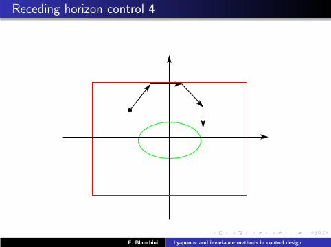
A possible solution: use invariant sets!
minJ =k+T−1
∑i=k
g(x(i),u(i))
s.t.
x(i +1) = f (x(i),u(i))
u(i) ∈ U , x(i) ∈ X , i = k ,k+1, . . . ,k+T −1,
x(k+T ) ∈ P
P controlled invariant.
F. Blanchini Lyapunov and invariance methods in control design

logo
Receding horizon control 3
A possible solution: use invariant sets!
minJ =k+T−1
∑i=k
g(x(i),u(i))+h(x(T ))
s.t.
x(i +1) = Ax(i)+Bu(i)
u(i) ∈ U , x(i) ∈ X , i = k ,k+1, . . . ,k+T −1,
x(k+T ) ∈ P
P controlled invariant.
F. Blanchini Lyapunov and invariance methods in control design

logo
Receding horizon control 4
F. Blanchini Lyapunov and invariance methods in control design

logo
Receding horizon control 4
F. Blanchini Lyapunov and invariance methods in control design

logo
Receding horizon control 4
F. Blanchini Lyapunov and invariance methods in control design

logo
Receding horizon control 4
F. Blanchini Lyapunov and invariance methods in control design
logo
Receding horizon control 4
F. Blanchini Lyapunov and invariance methods in control design

logo
Receding horizon control 4
F. Blanchini Lyapunov and invariance methods in control design

logo
Receding horizon control 4
F. Blanchini Lyapunov and invariance methods in control design

logo
Receding horizon control 5
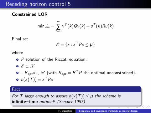
Constrained LQR
minJ∞ =∞
∑t=0
xT (k)Qx(k)+uT (k)Ru(k)
Final setE = x : xTPx ≤ µ
where
P solution of the Riccati equation;
E ⊂ X
−Koptx ∈ U (with Kopt = BTP the optimal unconstrained).
h(x(T )) = xTPx
F. Blanchini Lyapunov and invariance methods in control design
logo
Receding horizon control 5
Constrained LQR
minJ∞ =∞
∑t=0
xT (k)Qx(k)+uT (k)Ru(k)
Final setE = x : xTPx ≤ µ
where
P solution of the Riccati equation;
E ⊂ X
−Koptx ∈ U (with Kopt = BTP the optimal unconstrained).
h(x(T )) = xTPx
Fact
For T large enough to assure h(x(T ))≤ µ the scheme isinfinite–time optimal! (Sznaier 1987).
F. Blanchini Lyapunov and invariance methods in control design
logo
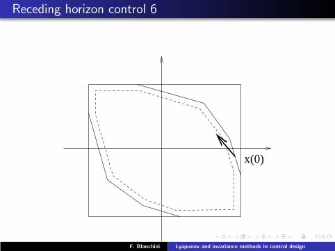
Receding horizon control 6
x(0)
F. Blanchini Lyapunov and invariance methods in control design

logo
Receding horizon control 6
x(0)
F. Blanchini Lyapunov and invariance methods in control design

logo
Receding horizon control 7
X
P
F. Blanchini Lyapunov and invariance methods in control design

logo
Receding horizon control 8
Final state weight g(x(T));
Cost–to–go function;
Explicit LQ solution (piecewise affine control) Bemporad,Morari, Dua, Pistikopulos (2002).
Multiparametric programming Mayne, Morari, Bemporad,Borrelli, Rakovic, Filippi, Johansen, Jones, Pistikopulos .....
F. Blanchini Lyapunov and invariance methods in control design

logo
Receding horizon control 9
Disturbances
Blanchini (1991), Mayne, Rakovic and Seron (2005), Mayne,Rakovic, Findeisen and Allgower (2006)
F. Blanchini Lyapunov and invariance methods in control design

logo
Receding horizon control 9
Disturbances
Blanchini (1991), Mayne, Rakovic and Seron (2005), Mayne,Rakovic, Findeisen and Allgower (2006)
F. Blanchini Lyapunov and invariance methods in control design

logo
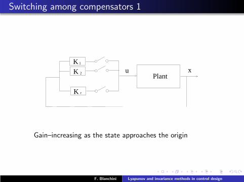
Switching among compensators 1
Plant
K
K
K
1
2
r
xu
F. Blanchini Lyapunov and invariance methods in control design
logo
Switching among compensators 1
Plant
K
K
K
1
2
r
xu
Gain–increasing as the state approaches the origin
F. Blanchini Lyapunov and invariance methods in control design

logo
Switching among compensators 1
Plant
K
K
K
1
2
r
xu
Gain–increasing as the state approaches the origin
Question: how can we switch in a safe way?
F. Blanchini Lyapunov and invariance methods in control design

logo
Switching among compensators 2
A possible solution: associate an invariant set with each gain.Construct these invariants sets in such a way they are nested.Then the scheme converges.
SS
S
1
2
r
F. Blanchini Lyapunov and invariance methods in control design

logo
Switching among compensators 3
But: You need state feedback or a reliable observer!
k
k
k
1
2
r
OBSERVER
PLANT
F. Blanchini Lyapunov and invariance methods in control design

logo
Switching among compensators 4
Example
y(t)+µ(t)y(t)+ y(t) = 0
the friction µ is the control constrained as 0.1≤ µ ≤ 10.
Damping control strategies
F. Blanchini Lyapunov and invariance methods in control design

logo
Switching among compensators 4
Example
y(t)+µ(t)y(t)+ y(t) = 0
the friction µ is the control constrained as 0.1≤ µ ≤ 10.
Damping control strategies
Constant: e.g. minimum/maximum/critical damping;
F. Blanchini Lyapunov and invariance methods in control design

logo
Switching among compensators 4
Example
y(t)+µ(t)y(t)+ y(t) = 0
the friction µ is the control constrained as 0.1≤ µ ≤ 10.
Damping control strategies
Constant: e.g. minimum/maximum/critical damping;
Heuristic switching: maximum damping when |y | ≤ ε, elseno–damping;
Invariant–set–based switching.
F. Blanchini Lyapunov and invariance methods in control design

logo
Switching among compensators 5
y
y
Figure: Heuristic strategy (blue) and the invariant–set–based strategy(red)
F. Blanchini Lyapunov and invariance methods in control design

logo
Switching among compensators 5
y
y
Figure: Heuristic strategy (blue) and the invariant–set–based strategy(red)
F. Blanchini Lyapunov and invariance methods in control design

logo
Switching among compensators 6
−2 −1.5 −1 −0.5 0 0.5 1−2
−1.5
−1
−0.5
0
0.5
1
1.5
2
Figure: State–space evolution of the heuristic strategy (dashed) and theinvariant–set–based strategy (plain)
F. Blanchini Lyapunov and invariance methods in control design

logo
Switching among compensators 7
0 1 2 3 4 5 6 7 8 9 10−2
−1.5
−1
−0.5
0
0.5
1
1.5
2
undamped
overdamped
critically damped
heuristic
switched
Figure: Performances of the considered strategies
F. Blanchini Lyapunov and invariance methods in control design

logo
Obstacle avoidance 1
F. Blanchini Lyapunov and invariance methods in control design

logo
Obstacle avoidance 1
Tracking a reference in environments with obstacles;
F. Blanchini Lyapunov and invariance methods in control design

logo
Obstacle avoidance 1
Tracking a reference in environments with obstacles;
Avoid collisions due to human errors;
F. Blanchini Lyapunov and invariance methods in control design

logo
Obstacle avoidance 1
Tracking a reference in environments with obstacles;
Avoid collisions due to human errors;
Covering by a family of connected controlled–invariant setswith ”crossing points”.
F. Blanchini Lyapunov and invariance methods in control design

logo
Obstacle avoidance 1
Tracking a reference in environments with obstacles;
Avoid collisions due to human errors;
Covering by a family of connected controlled–invariant setswith ”crossing points”.
Hierarchical controlLower level: in each set reaching the crossing point to thenext one (or the reference).Upper level: decision about the sequence of sets to becrossed;
F. Blanchini Lyapunov and invariance methods in control design

logo
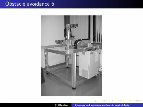
Obstacle avoidance 2
q2
q1
Figure: A manipulator in a constrained environment
F. Blanchini Lyapunov and invariance methods in control design

logo
Obstacle avoidance 3
Figure: The admissible region in the configuration set and itsapproximate covering
F. Blanchini Lyapunov and invariance methods in control design

logo
Obstacle avoidance 3
Figure: The admissible region in the configuration set and itsapproximate covering
F. Blanchini Lyapunov and invariance methods in control design

logo
Obstacle avoidance 4
Figure: The upper level control is a graph
F. Blanchini Lyapunov and invariance methods in control design
logo
Obstacle avoidance 6
F. Blanchini Lyapunov and invariance methods in control design

logo
Obstacle avoidance 7
F. Blanchini Lyapunov and invariance methods in control design
logo
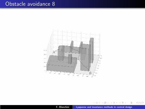
Obstacle avoidance 8
B
A
F. Blanchini Lyapunov and invariance methods in control design

logo
Conclusions
By means of set–invariance methods one can achieve several goals,especially if applied to special problems of practical importanceincluding
F. Blanchini Lyapunov and invariance methods in control design

logo
Conclusions
By means of set–invariance methods one can achieve several goals,especially if applied to special problems of practical importanceincluding
Overcoming the limits of linear compensators by properlyintroducing nonlinearities in the loop;
Supporting receding–horizon techniques;
Improving performances by combining compensators andswitching among them;
Solving constrained problems efficiently such as tracking andcollision avoidance;
Having fun with mathematics....
Too many others to be all included here!
F. Blanchini Lyapunov and invariance methods in control design

logo
The end
F. Blanchini Lyapunov and invariance methods in control design

logo
The end
Merci!
F. Blanchini Lyapunov and invariance methods in control design