luísa dechichi - universiteit twente · port and channel sedimentation: quantifying uncertainties...
TRANSCRIPT

PORT AND CHANNEL SEDIMENTATION: QUANTIFYING
UNCERTAINTIES USING AN EMULATOR
Luísa Dechichi
MSC Thesis
in Civil Engineering and Management


PORT AND CHANNEL SEDIMENTATION: QUANTIFYING
UNCERTAINTIES USING AN EMULATOR
Msc Thesis
In Civil Engineering and Management
Supervised by the
Department of Water Engineering and Management of University of Twente
&
Coastal, Harbour and Offshore Department of Deltares
Delft, Friday August 19th, 2016
To be presented on
Enschede, Friday 26th August, 2016
Graduation Committee:
Prof. dr. S.J.M.H. Hulscher (University of Twente, Graduation Supervisor)
ir. K.D. Berends (University of Twente/Deltares, Daily Supervisor)
ir. F. Scheel (Deltares, Daily Supervisor)
ir. W. de Boer (Deltares)
Prof. dr. Rosh Ranasinghe (UNESCO/IHE)


i
_____________________________________________________________________________________________________
Abstract _____________________________________________________________________________________________________
All around the world, expensive computationally models have been used in feasibility studies in order
to predict the amount of port siltation in a certain area. Depending on how many millions of cubic
meters of fine sediments brought into the navigation channel (by the tides, waves and rivers) need to
be dredged, the construction of such a port can become impractical due to high maintenance costs.
But if the uncertainties associated with this natural process are taken into account, for a better
prediction, then those models cannot be used due to the many runs required to compute these
uncertainties. The goal of this study is to quantify these uncertainties in port siltation using an
emulator. An emulator is a simpler model which aims to generate an output as close as possible from
the original model but with a lower computational time.
In order to reach the goal of this study, a model and two emulators with a lower horizontal resolution
will be used. The model and the two emulators are termed as sixteen grid cells model, eight grid cells
model and four grid cells model due to the number of grid cells along their respective navigation
channel width. Moreover, four steps will be applied as follows. Firstly, the uncertain input parameters
are selected with help of expert judgement and literature review. Secondly, we choose the one-at-a-
time method (OAT) to determine among the uncertain parameters which contributed most to the
uncertain in the model output, named as qualitative sensitivity analysis. Thirdly, we apply the Latin
Hypercube Sampling method (LHS) to sample the previously selected input parameters which are
used in the model runs for uncertainty quantification. Finally, we investigate mapping functions that,
along with the emulator, are capable to translate the amount of uncertainty in port siltation computed
by the model.
Regarding the sensitivity analysis, the uncertain input parameters to which the siltation is the most
sensitive are: bed roughness, settling velocity and significant wave height, according to the model and
the two emulators. However, the four grid cell model presented very low siltation values when
compared to the sixteen and eight grid cells models. Because of this, it is not used in uncertainty
quantification. With respect to the uncertainty quantification, the eight grid cells model present a
smaller amount of uncertainty in the model output when compared to the sixteen grid cells model.
This is an unrealistic result proving that the eight grid cells emulator cannot be used for uncertainty
quantification. As for the identification of mapping functions, four mapping functions are identified and
verified through box plots.
From this study, three important conclusions can be higlighted. First, the eight grid cells model is a
good replacement for the sixteen grid cells model with respect to siltation computation in the
navigation channel. Second, the four grid cells model can be used for a ‘parameter screening’ in
qualitative sensitivity analysis. Third, the eight grid cell model can be used for uncertainty
quantification if the specified mapping functions are applied. Summarizing, it is possible to quantify
the uncertainty in a navigation channel using an emulator as long as a mapping function is applied.
With attention to the fact that the channel width should be around 10 grid cells, otherwise the
hydrodynamics and morphodynamics are not well represented by the emulator.
Keywords: uncertainty analysis, sensitivity analysis, emulator, Delft3D, mapping function.

ii

iii
____________________________________________________________________________________________________
Preface & acknowledgments _____________________________________________________________________________________________________
“Valeu a pena? Tudo vale a pena
Se a alma nao é pequena.”
Fernando Pessoa, Mensagem (1934)
These verses are from Mar Português, one the one of the most famous poems of Fernando Pessoa,
in which the poet describes the story of the Portuguese navigators who left all behind in search of new
possibilities. In these verses he wonders “Was it worth it? All is worthwhile, if the soul is not small”.
This is exactly the feeling of gratitude that I have after going through this journey called master thesis.
Throughout these six months there were moments of rough seas, but also of calm waters. Everything
started two years ago in a land far away from here known as Brazil. Despite of the sadness of leaving
my family and friends behind, the challenging of a new adventure in The Netherlands, a country
different in so many aspects from mine, spoke louder. Here, every day has been a constant lesson
contributing to make me a better professional and human being. This master thesis marks the end of
this adventure and the start of a new one. But I cannot end this journey without thanking from all my
heart the people and institutions which made this dream come true.
First of all, I would like to thank my family specially my mother, father and sister who in spite of their
huge affection for me let me go to achieve my dream. Thanks for being always so supportive.
I acknowledge the University of Twente for supporting my dream with the University of Twente
scholarship, without it nothing of this would have ever been possible.
I would like to thank my supervisors Freek, Koen, Rosh, Suzanne and Wiebe for the priceless help
and guidance. I am going to miss the meetings and talks that added me so much and made me like
even more my project. Thanks for giving me this project which I felt in love from the very beginning.
Special thanks to Carles and Redmar for always been there for me and for their immense help,
support and patience during my thesis. I will be forever grateful. Also thanks to my friends in
Enschede and Delft for the relaxing and chilling moments of everyday life which made my stay in The
Netherlands much nicer.

iv
____________________________________________________________________________________________________
Contents ____________________________________________________________________________________________________
Abstract ................................................................................................................................ i
Preface & acknowledgments ............................................................................................. iii
1 Introduction ...................................................................................................................... 1
1.1 Background ................................................................................................................. 1
1.2 Research objectives .................................................................................................... 2
1.2.1 Knowledge gap ..................................................................................................... 2
1.2.2 Study case ............................................................................................................ 3
1.2.3 Model study ........................................................................................................... 4
1.3 Research objective ...................................................................................................... 7
1.4 Research questions ..................................................................................................... 7
2 Coastal morphodynamic modelling ................................................................................ 8
2.1 Hydrodynamic processes ............................................................................................ 8
2.2 Sediment transport .................................................................................................... 10
2.3 Channel sedimentation .............................................................................................. 11
2.4 Uncertainties ............................................................................................................. 11
3 Methodology ................................................................................................................... 13
3.1 Identification of uncertainty sources ........................................................................... 14
3.2 Performing sensitivity analysis ................................................................................... 14
3.3 Characterizing (relevant) uncertainty sources ............................................................ 15
3.4 Selecting uncertainty quantification method ............................................................... 16
3.5 Uncertainty quantification .......................................................................................... 18
3.6 Identifying mapping function ...................................................................................... 18
4 Results ............................................................................................................................ 19
4.1 Identification of uncertainty sources ........................................................................... 19
4.2 Performing sensitivity analysis ................................................................................... 20
4.3 Characterizing (relevant) uncertainty sources ............................................................ 20
4.3.1 Investigation ........................................................................................................ 24
4.4 Selecting uncertainty quantification method ............................................................... 25
4.5 Uncertainty quantification .......................................................................................... 26
4.6 Identifying mapping function ...................................................................................... 30

v
5 Discussion ...................................................................................................................... 34
6 Conclusion ..................................................................................................................... 35
7 Recommendation ........................................................................................................... 36
References ........................................................................................................................ 37
Appendix 1: Subjective sensitivity .................................................................................. 40
Appendix 2: Sensitivity analysis ...................................................................................... 42
Appendix 3: Latin Hypercube samples ............................................................................ 43
Appendix 4: Investigation of the maximum bed shear stress due to currents and
waves, the bed shear stress due to currents, the orbital velocity and the horizontal
velocity at the bed ............................................................................................................. 55
Appendix 5: Comparison between maximum bed shear stress due to currents and
waves, bed shear stress due to currents, orbital velocity and horizontal velocity at the
bed ..................................................................................................................................... 63

1
__________________________________________________________________________________
1 Introduction __________________________________________________________________________________
1.1 Background
Many ports around the world suffer from siltation on their berthing and manoeuvring areas, requiring
maintenance dredging activities to restore navigable depths (see Figure 1). Sedimentation of harbour
basins and navigation channels is a serious problem. Maintenance costs are a critical element in the
economic feasibility of a port, particularly when a relatively long access channel requires frequent
dredging. The maintenance dredging requirement for large sea ports and navigation channels may
exceed tens of millions m3/year of sediment removal (Deltares, 2011).
Figure 1: Dredging of the Port of Fremantle's Shipping Channels, 2010, Perth, Australia. (Becker, et al., 2013)
Due to the expensive maintenance of ports, predictions of port sedimentation are an important factor
for the feasibility study of building a port in a certain area. Many studies have been conducted using
empirical, numerical and physical models to study sedimentation processes in ports and channels
both qualitatively and quantitatively. However, modelling such processes is not an easy task, partly
due to the several known and unknown uncertainties in both the model input and within the model
itself, which later are translated into the model output.
Scientific decision support can provide assistance to policymakers in order to make decisions, while
taking into account uncertainties surrounding that decision (Walker, et al., 2003). The identification
and quantification of these uncertainties (known as uncertainty analysis) usually requires many model
Chapter 1 Introduction 2
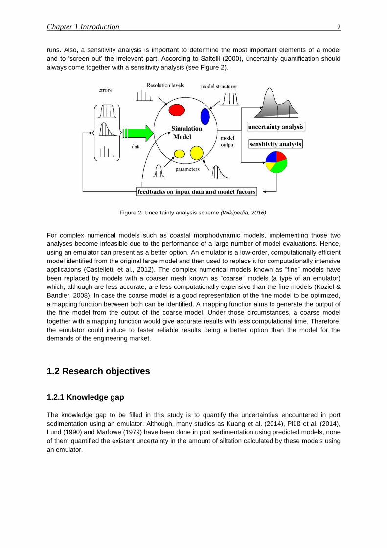
runs. Also, a sensitivity analysis is important to determine the most important elements of a model
and to ‘screen out’ the irrelevant part. According to Saltelli (2000), uncertainty quantification should
always come together with a sensitivity analysis (see Figure 2).
Figure 2: Uncertainty analysis scheme (Wikipedia, 2016).
For complex numerical models such as coastal morphodynamic models, implementing those two
analyses become infeasible due to the performance of a large number of model evaluations. Hence,
using an emulator can present as a better option. An emulator is a low-order, computationally efficient
model identified from the original large model and then used to replace it for computationally intensive
applications (Castelleti, et al., 2012). The complex numerical models known as “fine” models have
been replaced by models with a coarser mesh known as “coarse” models (a type of an emulator)
which, although are less accurate, are less computationally expensive than the fine models (Koziel &
Bandler, 2008). In case the coarse model is a good representation of the fine model to be optimized,
a mapping function between both can be identified. A mapping function aims to generate the output of
the fine model from the output of the coarse model. Under those circumstances, a coarse model
together with a mapping function would give accurate results with less computational time. Therefore,
the emulator could induce to faster reliable results being a better option than the model for the
demands of the engineering market.
1.2 Research objectives
1.2.1 Knowledge gap
The knowledge gap to be filled in this study is to quantify the uncertainties encountered in port
sedimentation using an emulator. Although, many studies as Kuang et al. (2014), Plüß et al. (2014),
Lund (1990) and Marlowe (1979) have been done in port sedimentation using predicted models, none
of them quantified the existent uncertainty in the amount of siltation calculated by these models using
an emulator.

Chapter 1 Introduction 3
1.2.2 Study case In the present study, a port feasibility study is proposed by a client of Deltares, an independent
institute for applied research in the field of water and subsurface. The client is interested in building a
port in a certain area, which can be represented as seen in Figure 3. The area is mainly composed by
mud and the transport of sediments is affected by the river discharge, waves and tidal flow. Due to
client’s request the location of the port cannot be revealed. This is irrelevant to the aim of this study.
Figure 3: Scheme of the study area.
Prior to building this port, the client wants to know the expected amount of annual siltation that is likely
to take place in the navigation channel, in relation to the future costs of maintenance that it would
require. The client is confronted with a range of possible amounts of future siltation. A distribution
representing this uncertainty range of siltation, such as (cumulative) distribution function, provides this
information (see Figure 4 as an example of cumulative distribution of annual amount of siltation).
Figure 4: Example of a cumulative probability function of siltation.
A cumulative distribution function (CDF) of a distribution function , evaluated at , is the probability
that will take a value less than or equal to . Thus, this example shows that the probability that the
annual amount of siltation will be less than or equal to 100x106 kg is of the 50%.

Chapter 1 Introduction 4
1.2.3 Model study
In this study, we simulate port sedimentation using Delft3D. Delft3D is an open source, flexible,
integrated modelling framework, developed by Deltares, simulating two and three-dimensional flow,
waves, sediment transport and morphology, water quality and ecology and is capable of handling
many interactions between these processes. Among the several modules of the software (see Figure
5) the used module is Delft3D-FLOW which is a multidimensional (2D or 3D) hydrodynamic simulation
program which calculates non steady flow and transport phenomena that result from tidal and
meteorological forcing on a rectilinear or curvilinear, boundary fitted grid.
Figure 5: Delft3D Modules. (Deltares, 2014)
The original model can be found in Figure 6. The navigation channel has a depth of 20m MSL. The
Boundary Conditions (BC’s) consist of offshore tidal elevation on the left and the river discharge
flowing into the system towards the navigation channel. The Initial Conditions (IC’s) are: 0.25 m for
water level, 35 ppt for salinity and 0 kg/m3 for concentration of mud.
Figure 6: Schematization of the model.
In this study, three Delft3D models will be used, varying in number of horizontal grid cells. All models
have eight layers over the vertical. The original model has sixteen grid cells over the width of the
navigable channel, while the emulators feature eight and four grid cells. In order to differentiate from
the two emulators, one will be called eight grid cells model and the other four grid cells model. The
original model will be called sixteen grid cells model. Figure 7 shows a plan view of the three models
where the navigable channel lies within the depicted red rectangle: it consists of sixteen, eight and
four grid cells in the y-direction for the sixteen grid cells model, eight grid cells model and the four grid
cells model, respectively.
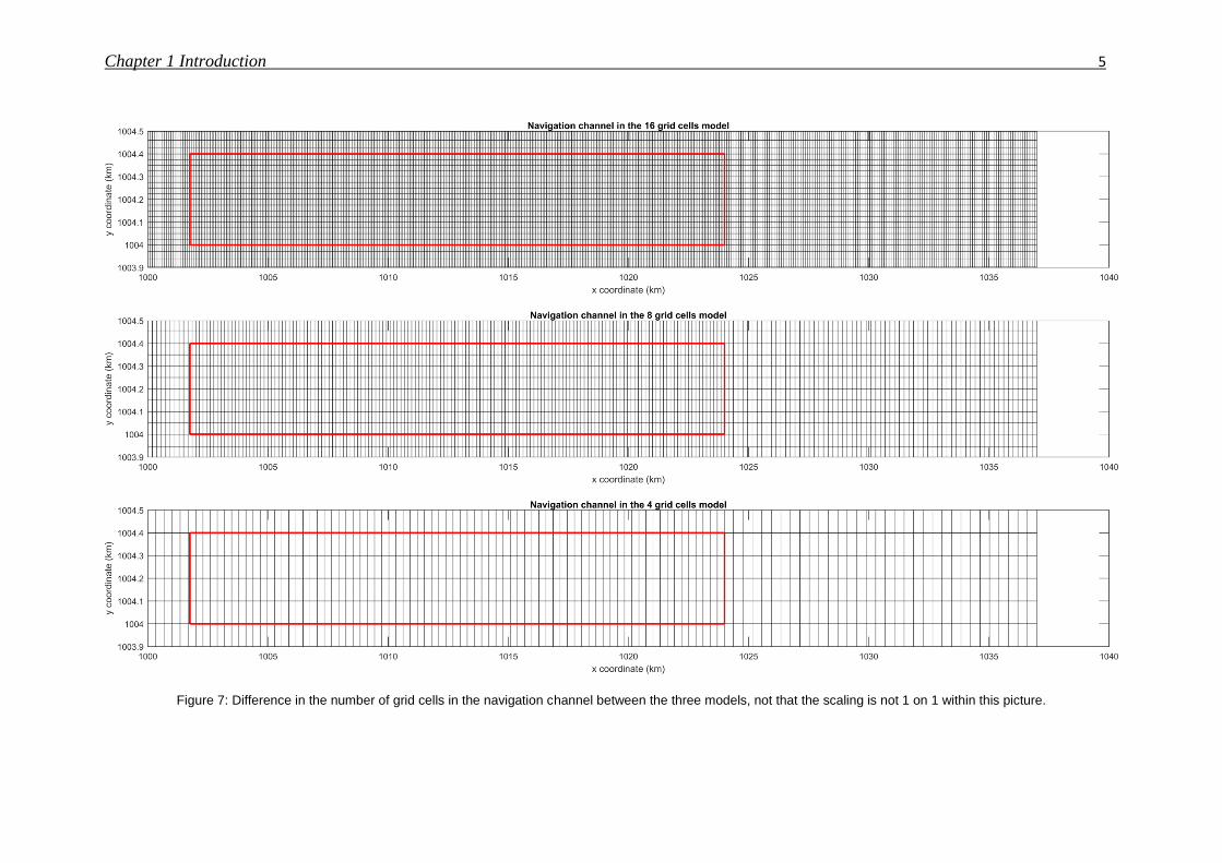
Chapter 1 Introduction 5
Figure 7: Difference in the number of grid cells in the navigation channel between the three models, not that the scaling is not 1 on 1 within this picture.

Chapter 1 Introduction 6
In the particular case analysed, sedimentation processes are mainly driven by currents (flow) and wind waves. These processes will be modelled in Delft3D by using the ‘Flow’ and ‘Wave’ modules (see Figure 8). These modules can be run simultaneously in the so-called ‘online-coupling’ mode, which allows interaction between the modules with a coupling interval that was set to one hour. The updated bottom, water level and velocity information are passed to the wave model and wave-induced forces, wave heights, periods and directions are returned to the flow module. For the purpose of this study, it was decided not to update the bathymetry because it is assumed that the port will be dredged continuously for maintenance purposes.
Figure 8: General chart of Deflt3D system. Adapted from (Roelvink & Walstra, 2005)
Besides the hydrodynamic grid, there is also a wave grid defined in the Delft3D-WAVE for each of the three models. Figure 9 shows the wave and hydrodynamic grids defined in Delft3D-WAVE and Delft3D-FLOW, respectively. The wave grid is bigger than the hydrodynamic grid in order to guarantee that the wave information will be passed to the flow grid without problems.
Figure 9: Wave grid (blue) and hydrodynamic grid (red) for the sixteen grid cells model.

Chapter 1 Introduction 7
As the bathymetry is not updated, the quantification of the amount of siltation in the channel is
computed through the available mass within the uniform bed. The type of bed adopted is a uniformly
well-mixed bed consisting of one layer of non-depleting muddy sediment. All the sediment is available
for erosion. When sediments are deposited, they are added to the layer and when sediments are
eroded, the layer exports sediments to the water column.
1.3 Research objective The objective of this study is:
Can an emulator help estimating the uncertainty of navigation channel siltation in a guide and robust
way?
Naturally there are several limitations and assumptions. First of all, the following study is applicable
for a Delft3D model, which will be considered sufficient to represent the morphodynamic and
hydrodynamics processes in port siltation. Second, the model and the emulators differ in the number
of gridcells, while the underlying relations for hydrodynamic and morphodynamic processes are the
same in both original and emulators models. At last, the chosen intervals for the parameters also
restrict the applicability of this study.
1.4 Research questions
The goal is to answer the following research questions:
1. What are the uncertain input parameters with respect to a coastal morphodynamic model?
2. What are the most sensitive uncertain input parameters for a Delft3D model?
3. In what way does the amount of uncertainty in siltation differ between model and emulator?
4. Can a mapping function be applied to the emulators in order to map the amount of uncertainty
in the siltation distribution computed by the model?
8
____________________________________________________________________________________________________
2 Coastal morphodynamic modelling ____________________________________________________________________________________________________
When modelling a coastal environment, several difficulties need to be taken into account. First, the
interaction between hydrodynamics and sediment is very complex and poorly understood (Vollmers,
1989). Besides that, several of the parameters cannot have their values determined from the site due
to factors like low budget for data acquisition, difficulty in measuring or its random behaviour. Despite
all these difficulties it is still possible to make reasonable predictions of the expected amount of
siltation in navigable channels, for example. A brief explanation about the hydrodynamic processes,
sediment transport, siltation and uncertainties will be given in this chapter in order to make clear for
the reader the steps taken towards the goal of this study.
2.1 Hydrodynamic processes The nearshore hydrodynamics are important for sediment transport due to their capacity of stirring up
sediments from bed and transport them along the surf zone. When waves come from deep to shallow
waters, their characteristics as wave height and direction change. Shallow water processes include
shoaling, wave breaking, wave orbital velocities and bed shear stress, which are the most relevant for
the present work.
When waves come from deep water propagate perpendicularly towards the coast and reach a water
depth less than about half the wavelength, their speed slows down due to the bed shear stress.
Considering energy conservation, as the velocity goes down, the wave height increases: the waves
experience shoaling. The ratio between wave height and wave length is called wave steepness.
However, this increase in height is controlled by the dissipation due to wave breaking. The wave
breaking occurs when the particle velocity exceeds the velocity of the wave crest causing the wave
crest to become unstable.
Under wave surface, fluid particles describe an orbital path. Ideally, from the water surface to the
bottom their trajectory changes from circular to ellipsoidal. At the same time, orbital diameter
becomes smaller further down from the surface. Above the bed there is a turbulent layer called wave
boundary layer which is approximately 5 to 10 cm. This turbulence is enhanced by bed roughness in
combination with high flow orbital velocities. In this layer, the orbital velocity is responsible for varying
the bed shear stress during the time which can set sediments on the bed into motion. The orbital
velocity is zero at the bed and is equal to non-zero wave-averaged horizontal velocity (free-stream
velocity) at the top of the layer. This velocity which has the same direction as wave propagation is
extremely important for the transport of sediment onshore.
Accordingly, bed shear stress occurs due to currents and to waves. In order to determine the bed
shear stress due to waves, Jonsson (1966) came up with the concept of wave friction factor which is a
similar concept used to calculate the bed shear stress due to currents. However, while current friction
factor is related to depth averaged current velocity, wave friction factor is related to free-stream
velocity. The bed shear stress due to currents can be calculated as follows:
| ⃗⃗ | ⃗⃗ (1)
(2)
| ⃗⃗ | | ⃗⃗ |
(
) (3)
Chapter 2 Coastal morphodynamic modelling 9
where is the bed shear stress due to currents, is the current friction factor, is the density of
water, ⃗⃗ is the depth-averaged flow velocity, g is the gravity and C is the Chézy friction coefficient , ⃗
is friction velocity due to currents and waves and is bed roughness length.
In this study, the bottom roughness will be computed using the Manning’s formulation. For a constant
Manning value the bottom roughness increases rapidly with decreasing depth. As a result, the flow
will be shifted to deeper water and the velocities nearshore will be reduced. This will greatly affect the
longshore sediment transport.
√
(4)
where is the Manning coefficient in , is the water depth in . The magnitude of the wave-
averaged bed shear-stress due only to waves is
| |
(5)
where is the magnitude of the bed stress for waves alone in , is the reference density of
water in , is the total friction wave factor and the is the orbital velocity in . For the
orbital velocity the following formulation is used:
√
(6)
and is the square root of the wave height in m1/2
, is the wave angular frequency in s-1
, k is the
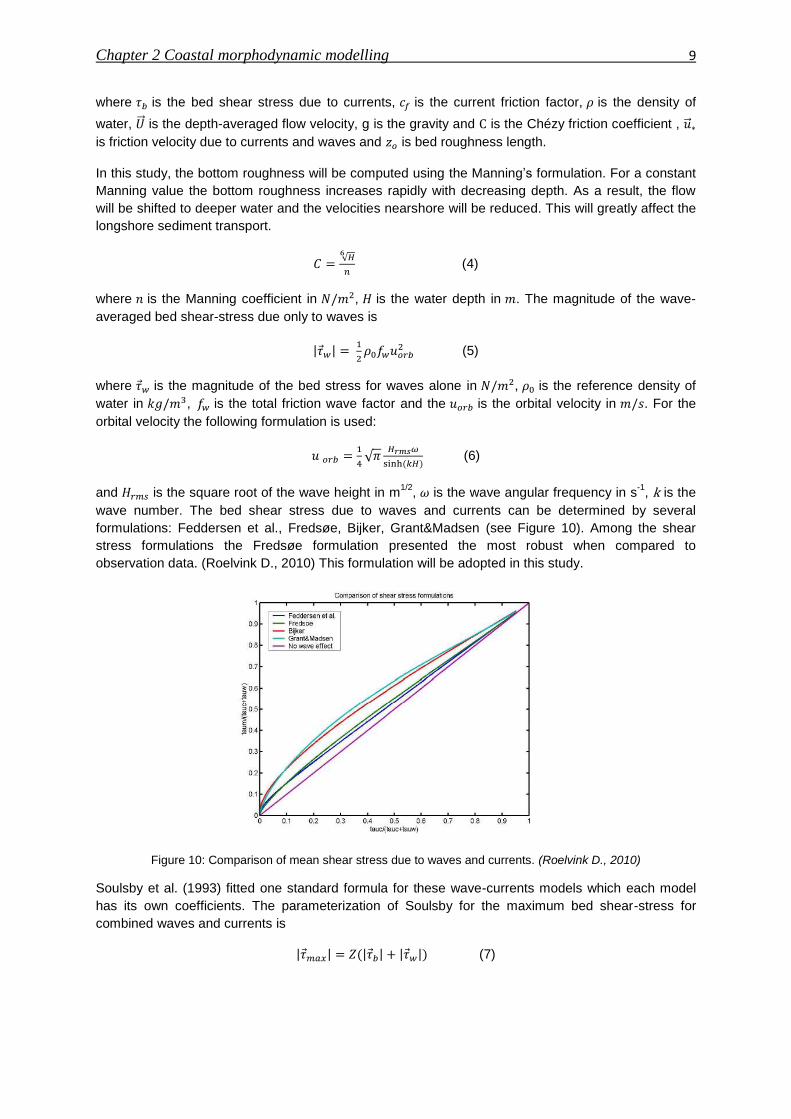
wave number. The bed shear stress due to waves and currents can be determined by several
formulations: Feddersen et al., Fredsøe, Bijker, Grant&Madsen (see Figure 10). Among the shear
stress formulations the Fredsøe formulation presented the most robust when compared to
observation data. (Roelvink D., 2010) This formulation will be adopted in this study.
Figure 10: Comparison of mean shear stress due to waves and currents. (Roelvink D., 2010)
Soulsby et al. (1993) fitted one standard formula for these wave-currents models which each model
has its own coefficients. The parameterization of Soulsby for the maximum bed shear-stress for
combined waves and currents is
| | | | | | (7)

Chapter 2 Coastal morphodynamic modelling 10
2.2 Sediment transport
Sediment transport is a crucial bond between waves, currents and morphological changes. It is
related with current, orbital velocities, sediment properties, bed forms and bed roughness. The
sediment transport can be divided into bed load transport and suspended load transport. The bed
load transport takes place through sediments which roll, shift or make small jumps over the seabed,
staying in contact with the bed. The suspended load transport occurs via sediments which are lifted
up above the critical flow velocity and are transported in suspension by the flow. If the flow velocity
decreases until a certain value, then the suspended sediments settle down.
As previously mentioned, the sediment transport is related to the sediment properties. In fact, the
sediments can be divided into two main groups: cohesive and non-cohesive. This classification is
important to sediment transport because the upward sediment flux from the bed into the water column
strongly depends on the bed cohesiveness. This cohesiveness is related to the capacity of certain
materials to stick together due to chemical constitution which will increase greatly the resistance
against erosion. Sand is a non-cohesive material while silt, clay and organic materials are cohesive
materials. The fluid-sediment mixture of (salt) water, silt, clay and organic materials known as mud is
a cohesive material.
The upward sediment flux from the bed into the water column is commonly accepted to be controlled
by the critical bed shear stress of the bed material and the actual bed shear stress. If the actual bed
shear stress is bigger than the critical bed shear stress, erosion will take place. On the other hand, if
the actual bed shear stress is smaller than the critical bed shear stress, deposition will take place. In
case of non-cohesive sediments, the critical bed shear stress for erosion and sedimentation are the
same. As a result, the transport of sand can be well predicted by empirical sediment transport
formulas as Van Rijn, Engelund-Hansen and Meyer-Peter-Muller. In case of cohesive materials, the
critical bed shear stress for erosion is larger than the critical bed shear stress for sedimentation. In
case the actual bed shear stress is between the critical bed shear stress for erosion and for
sedimentation there will be no exchange with the bottom layer. In fact, it is not commonly accepted
the existence of a critical shear stress for deposition (Winterwerp, 2004).
According to Eq. 8 it can be observed that the change of the bed level is controlled by the rate of
deposition and erosion:
(8)
[
] (9)
[
] (10)
where is the porosity, and are the sediment transport in the x- and y-direction, D is the
deposition rate of suspended sediment, E is the erosion rate of suspended sediment, M is the erosion
parameter, is the actual critical bed shear stress, is the critical bed shear stress for erosion,
is the critical bed shear stress for sedimentation, is the settling velocity and C is the
concentration of sediments in the water column.
In a coastal environment the sediment transport on cross-shore and alongshore direction has an
important role on the morphodynamics system. Wave orbital motion is very important for the sediment
transport on cross-shore direction. This type of sediment transport is essential to stir up the sediments
and keep them into suspension in the water column. But it does not contribute to actually transport
these sediments along the coast. That is done by the alongshore sediment transport. Regarding it, the

Chapter 2 Coastal morphodynamic modelling 11
wave-induced surf zone longshore flow is important because it produces a longshore current along
the coast. The wave-induced flow is determined by wave characteristics as wave height, period and
direction.
2.3 Channel sedimentation
In ports the navigable channels unfortunately work as ‘sediments trap’ which increases the
maintenance costs due to the need of maintaining the required channel depth for the ships to enter in
the port. In the channel the velocities become smaller due to the higher water depth, causing a
reduction in the sediment transport capacity. Consequently, the bed load particles and part of the
suspended load particles will be deposited in the channel. In addition, the gravitational effect induces
a downward force on bed-load particles on the side slopes of a channel. On the other hand, the
dynamic nature of the channels produces shifting shoals and banks (Van Rijn, 2013). Figure 11
shows the main factors responsible for the sedimentation in a navigation channel. For the studied
navigation channel, the currents caused by tides and waves also approach alongside the channel as
showed in Figure 11.
Figure 11: Channel sedimentation. Adapted from (Van Rijn, 2005).
If the waves are included then more sediment is expected to be deposited in the channel due to the
capacity of the waves to stir up sediments which will be transported by the flow. Therefore, the
amount of sedimentation that may take place in a navigable channel depends on the rate of sediment
transport, which is controlled by the flow, the waves, the sediments approaching to the channel, and
the trapping efficiency of the channel influenced by the geometry, dimensions, channel orientation
and the sediment characteristics.
2.4 Uncertainties
Although the idea of uncertainty is quite familiar to most of the people its sources are not always easy
to identify. A general definition of uncertainty would be: “a situation in which something is not known,
or something that is not known or certain” (Cambridge, 2016). But in environmental modelling, in his
first chapter brings two classical definitions of uncertainty: one derived from set theory and one from
statistics. Conforming to the first definition, uncertainty appears when there is a set of possible
alternatives when only one is required. And conforming to the second definition, there is a universal
set of alternatives which can be expressed in terms of some measure, in the range from 0 to 1. For
Beven (2009) both definitions have their limitations. After an overview of the various definition of
uncertainty, he observes that having a different definition will lead to different ways of representing

Chapter 2 Coastal morphodynamic modelling 12
sources of uncertainty in the modelling process, which in turn will result in different uncertainty
estimation of the model output. He conclude that in real applications the most important aspect of
uncertainty estimation is to make better decisions, and that different methods of uncertainty
estimation are necessary for different types of problems.
According to Scheel et al. (2014), the imperfect description of the physics in the model, the inability to
accurately define model input parameters and the natural variations in the model forcing have
introduced uncertainty in morphological model predictions. Therefore, identification and quantification
of those uncertainties is not only important to better understand the studied morphological system, but
also to be able the decision maker to take risks informed decisions. Fortunato et al (2009) also
realized the increase importance of uncertainty in determining the limits of predictability of
morphodynamics models due to the increase owed to the growing of computational resources. For
Scheel et. al. (2014) the sources of these uncertainties are (see Figure 12):
Forcing uncertainty: it is an inherent uncertainty in the forcing condition due to its natural
variation in space and time. For example: storms, disasters, climate changes, etc;
Parameter uncertainty: it is an uncertainty in (physical) model parameters. It occurs due to the
absence of enough data and knowledge about the empirical formulas, parameters
resemblance with reality, measurement techniques, initial conditions, etc;
Model uncertainty: it is an epistemological uncertainty due to the incompleteness of
conceptualizing a real system into a model. For example, errors in numerical methods,
underlying assumptions, limited processes, etc;
Unknown uncertainty sources: it is inherent uncertainty which comes from unknown and
unpredictable sources. For example, human errors, wrong assumptions, etc.
Figure 12: Sources of uncertainty in morphodynamics models. A) Forcing Uncertainty. B) Parameter uncertainty. C) Model uncertainty D) Unknown uncertainty sources (Scheel, et al., 2014).
As it can be noted, most of these uncertainties cannot be eliminated due to its inherent aspect of the
model or the system. However, the quantification of these uncertainties will contribute to make clearer
the limits of predictability of morphodynamics models for both decision makers and scientists.

13
__________________________________________________________________________________________________
3 Methodology ____________________________________________________________________________________________________
The methodology applied is based on the workflow suggested by Scheel et. al. (2014) is shown in
Figure 13. This workflow was expanded with the final step “Identifying mapping function” in order to
take into account the last step of this study.
Figure 13: Adopted uncertainty analysis workflow.
A brief overview of each step can be found in this chapter.
Identification of
uncertainty sources
(Research Question 1)
Performing sensitivity
analysis
Selecting uncertainty
quantification method
Performing simulations
Uncertainty quantification
(Research Question 3)
Characterizing (relevant)
uncertainty sources
(Research Questions 2)
Identifying mapping function
(Research question 4)

Chapter 3 Methodology 14
3.1 Identification of uncertainty sources
Numerical models need input parameters in order to give the output of interest. The number and type
of input parameters depend on the assumptions made by the modeller. The user is interested in
including all the input parameters which are relevant to describe the phenomenon analysed.
As it was mentioned before, modelling is not an easy task due to the uncertainties in many of its
aspects, including in the input. In order to deal with modelling uncertainties, a previous sensitivity
analysis and uncertainty analysis are recommended in several disciplines. While sensitivity analysis
focus on how uncertainty in the output of model can be apportioned to different sources of uncertainty
in the model input, the uncertainty analysis focus on quantifying these uncertainties in model output
(Baveye, et al., 2007) . The importance of sensitivity analysis in disciplines as applied econometrics is
illustrated by Peter Kennedy, who stated “Thou shall confess in the presence of sensitivity” which can
be translated into “Look at uncertainties before going public with findings”.
Among the several sources of uncertainty mentioned by Scheel et al. (2004), the parameter
uncertainty will be the focus of this study. In that case, it is necessary to take a look into the model
and identify the uncertain input variables. In Appendix 1, most of the input variables of the Delft3D-
FLOW and Online Delft3D-WAVES for the model are listed. Several input variables are constant (e.g.
gravity) and others were assumed to be constant (e.g. water density) for simplicity.
The first filter to eliminate non important parameters was the knowledge from an expertise who has
been modelling coastal areas during years and have gained insight on which parameters and
processes can be discarded due to their small influence on model results. In different areas the
subjective analysis has been showed to be a valuable tool for uncertainty analysis including Cooke, et
al. (2002), Morgan, et al. (1995) and Evans et al. (1994). In this study, this method was used in order
to reduce the number of input variables to a feasible size. In view of that, an interview with Freek
Scheel, a consultant and researcher in coastal engineer at Deltares, was carried out in order to
discuss the uncertain input parameters in a Delft3D coastal morphodynamics model. In addition, but
also a research in literature was done.
3.2 Performing sensitivity analysis
Here the goal is to analyse how much the model output is affected while changing the input variables.
For that, a sensitivity method is applied. From all existing sensitivity methods it was chosen to use the
one-at-a-time method (OAT). This method consists of varying one parameter at time while keeping
the others fixed (Hamby, 1994). The way in which the number and values of the parameters have to
be chosen is dependent on the type of model output of interest. For this study, the extreme values of
the variables (e.g 1st and 99
th percentiles) are not important. On the contrary, an overview of the
whole output distribution is more interesting. With this intention, while one variable is set to the 10th or
90th percentile of its distribution, the others will be left constant, by that, to the 50
th percentile of their
respective distribution as schematized in Figure 14.
Chapter 3 Methodology 15
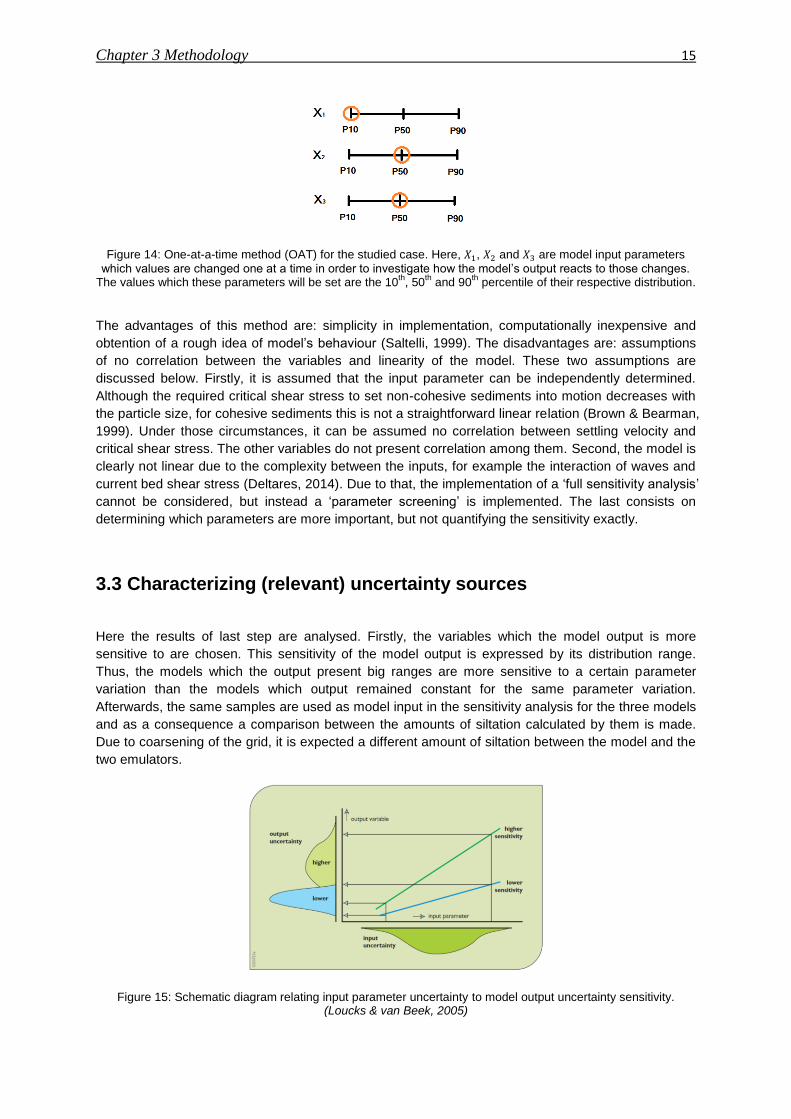
Figure 14: One-at-a-time method (OAT) for the studied case. Here, , and are model input parameters
which values are changed one at a time in order to investigate how the model’s output reacts to those changes. The values which these parameters will be set are the 10
th, 50
th and 90
th percentile of their respective distribution.
The advantages of this method are: simplicity in implementation, computationally inexpensive and
obtention of a rough idea of model’s behaviour (Saltelli, 1999). The disadvantages are: assumptions
of no correlation between the variables and linearity of the model. These two assumptions are
discussed below. Firstly, it is assumed that the input parameter can be independently determined.
Although the required critical shear stress to set non-cohesive sediments into motion decreases with
the particle size, for cohesive sediments this is not a straightforward linear relation (Brown & Bearman,
1999). Under those circumstances, it can be assumed no correlation between settling velocity and
critical shear stress. The other variables do not present correlation among them. Second, the model is
clearly not linear due to the complexity between the inputs, for example the interaction of waves and
current bed shear stress (Deltares, 2014). Due to that, the implementation of a ‘full sensitivity analysis’
cannot be considered, but instead a ‘parameter screening’ is implemented. The last consists on
determining which parameters are more important, but not quantifying the sensitivity exactly.
3.3 Characterizing (relevant) uncertainty sources
Here the results of last step are analysed. Firstly, the variables which the model output is more
sensitive to are chosen. This sensitivity of the model output is expressed by its distribution range.
Thus, the models which the output present big ranges are more sensitive to a certain parameter
variation than the models which output remained constant for the same parameter variation.
Afterwards, the same samples are used as model input in the sensitivity analysis for the three models
and as a consequence a comparison between the amounts of siltation calculated by them is made.
Due to coarsening of the grid, it is expected a different amount of siltation between the model and the
two emulators.
Figure 15: Schematic diagram relating input parameter uncertainty to model output uncertainty sensitivity. (Loucks & van Beek, 2005)

Chapter 3 Methodology 16
3.4 Selecting uncertainty quantification method
The uncertain quantification method chosen is the Latin Hypercube Sampling (LHS) which was
described by McKay et al. (1979). The LHS method is a type of Monte Carlo, a sampling method that
generates random samples from the probability distributions. The main advantage of LHS when
compared to crude Monte Carlo is the more equally division of the sample probability distribution in
order to guarantee that the whole probability distribution is sampled. First, the range of each variable
is divided into n non-overlapping intervals of equal probability called strata. After, the values of these
variables are randomly chosen in a way that each range is sampled only once. Later, these values
are randomly combined to n sets of Latin Hypercube samples. In the end, each of the n samples
contains only one value for each variable (see Figure 16).
Figure 16: Latin Hypercube Sampling scheme. (Van der Klis, 2003)
These samples work as different input scenarios for the model which will generate outputs equi-
distributed over the desired output distribution. Among the many advantages of LHS are :
1. Unbiased estimates for means and distribution functions;
2. Dense stratification across the range of each sampled variable;
3. Uncertainty and sensitivity analysis results obtained with Latin Hypercube sampling have
been observed to be quite robust even when using relatively small samples (i.e n = 50 – 200);
4. The means and distribution functions estimated tend to be more stable than in the Crude
Monte Carlo. In other words, the amount of variation between results obtained with different
samples generated by the particular samping technique under consideration is smaller.
The disadvantage is the fact that its accurancy cannot be measured differently than in the crude
Monte Carlo, which different formulations can be found in literature (Morgan & Henrion, 1990). For
that, it would be necessary to repeat the LHS several times and therefore, this would atenuate its
advantage of using a smaller sample size (Van der Klis, 2003).
It is necessary to choose intervals which the probability distribution of the variables will be divided
into equal probability. Initially the probability distribution of the most sensitive uncertain input
parameters was divided by and as a consequence that is also the number of the sample size.

Chapter 3 Methodology 17
Although there is no formulation which recommends the sample size for LHS, it can be found in
several studies as in Chang, et al. (1993), Yeah, et al. (1993), Christiaens, et al. (2001) and Van der
Klis (2003) that a sample size of 80 is a reasonable number.
Due to the different computational time of the models, different sample sizes were adopted. For a
single run, the sixteen grid cells model takes approximately three days, the eight grid cells model
takes around one day and the four grid cells model takes approximately five hours. Consequently, it is
not feasible to use a sample size of for the sixteen and eight grid cells model.
Thereupon the four grid cells model used the original sample size of 80 samples, while the eight grid
cells model and the sixteen grid cells model used subsamples of the original sample size of 40 and 20
samples. An example of LHS subsamples and from an original LHS sample can be
found in Figure 17.
Figure 17: Example of subsampling from LHS. A) It is the original LHS (n=8). B) It is a subsample of the original LHS (n=4). C) It is subsample of the last one (n=2).
Despite the different subsample sizes, both come from the original one. As a result, it is possible to
compare the cumulative distribution function of the siltation of the three models. The final LHS runs
can be found in the scheme in Figure 18. In this scheme, the columns represent the three sample
sizes initially adopted (80, 40 and 20 samples), the rows are the three models (sixteen grid cells
model, eight grid cells model and four grid cells model), the symbol represents the known siltation
data and the unknown siltation data.
Figure 18: Scheme for the LHS runs from the sensitivity analysis.
Chapter 3 Methodology 18
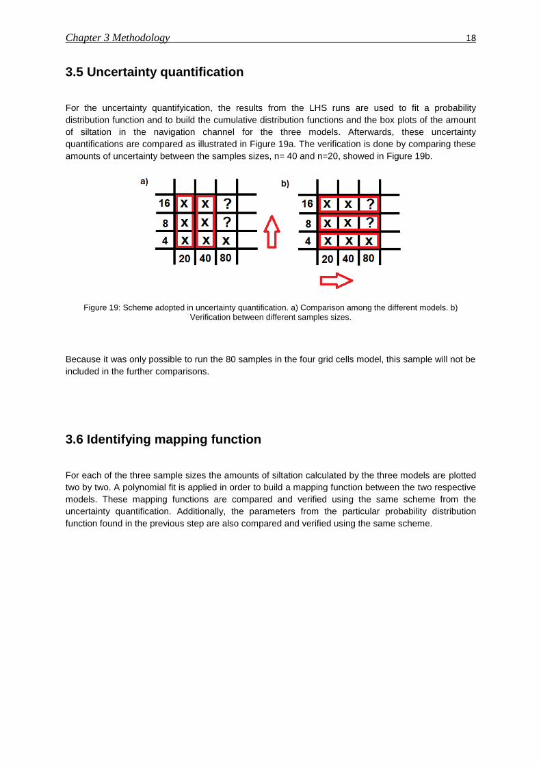
3.5 Uncertainty quantification
For the uncertainty quantifyication, the results from the LHS runs are used to fit a probability
distribution function and to build the cumulative distribution functions and the box plots of the amount
of siltation in the navigation channel for the three models. Afterwards, these uncertainty
quantifications are compared as illustrated in Figure 19a. The verification is done by comparing these
amounts of uncertainty between the samples sizes, n= 40 and n=20, showed in Figure 19b.
Figure 19: Scheme adopted in uncertainty quantification. a) Comparison among the different models. b) Verification between different samples sizes.
Because it was only possible to run the 80 samples in the four grid cells model, this sample will not be
included in the further comparisons.
3.6 Identifying mapping function
For each of the three sample sizes the amounts of siltation calculated by the three models are plotted
two by two. A polynomial fit is applied in order to build a mapping function between the two respective
models. These mapping functions are compared and verified using the same scheme from the
uncertainty quantification. Additionally, the parameters from the particular probability distribution
function found in the previous step are also compared and verified using the same scheme.

19
____________________________________________________________________________________________________
4 Results _________________________________________________________________________________
4.1 Identification of uncertainty sources
After the interview and the literature review, five uncertain input variables are chosen from the thirty
six input variables found in the two tables in Appendix 1. The uncertain input parameters can be found
in the following table:
Table 1: Uncertain input parameters.
Uncertain Parameter Unit P10 P50 P90 Data
Settling Velocity ms-1
0.1 0.5 1.0 Normal
Bed roughness Nm-2
0.018 0.020 0.22 Normal
Wave height m 0.71 1.20 1.30 Data-based
Discharge m3s
-1 0.24 1.24 110.60 Data-based
Critical Shear Stress for Erosion Nm-2
0.4 0.5 0.6 Normal
Table 1 also shows the type of data and the 10th, 50
th and 90
th percentiles of the probability
distribution or data series for each parameter. It was assumed that the settling velocity, bed
roughness and critical shear stress have a normal distribution. In relation to the wave height and the
discharge, time-series are provided by Deltares. Figure 20 and Figure 21 show the distribution and
the 10th, 50
th and 90
th percentiles for the wave height and the discharge, respectively. As previously
mentioned in ‘Study Case’ the location of the port cannot be revealed, and as consequence the same
applies to the locations where both time-series were measured.
Figure 20: Distribution of the wave height at port’s location.

Chapter 4 Results 20
Figure 21: Distribution of the discharge at port’s location.
4.2 Performing sensitivity analysis
Within the OAT method, 11 runs for each model were perfomed resulting in a total of 33 runs. For the
three model, a reference case was simulated in which all the uncertain input variables are set to their
median value of their respective distribution. The values used in the reference cases can be found in
Table 1. The run period is set from 01-07-2014 to 01-08-2014.
4.3 Characterizing (relevant) uncertainty sources
An error bar plot is generated in order to show the results from the sensitivity analysis. Figure 22
shows the different values of siltation inside of the channel when varying the bed roughness for the
four grid cells model. For example, if the value of bed roughness is set to its 10th percentile while the
other four uncertain input parameters are set to their median values, the siltation will be approximately
10.0 x 10⁶ kg (represented by the magenta line in Figure 22).
Figure 22: Error bar of the bed roughness for the four grid cells model.

Chapter 4 Results 21
Figure 23: Results from the sensitivity analysis using the OAT method.

Chapter 4 Results 22
From the sensitivity analysis results showed in Figure 23, three important conclusions can me made:
1. The three most sensitive parameters are the bed roughness, the settling velocity and
significant wave height. As it can be observed in Figure 23, the siltation is more sensitive to
the variation of the bed roughness than the critical shear stress. Given that, when the bed
roughness varies the amount of siltation becomes more distant from its reference value. As a
result, the siltation is more sensitivity to the bed roughness than to the critical shear stress.
The same happens to the settling velocity and the significant wave height. The three models
showed the same results.
2. It can be observed that two factors seem to dominate the output sensitivity: the
resolution (among the models) and the parameter range (among the parameters). Table
7 found in Appendix 2 brings the exact values of the total amount of siltation for the three
models obtained in the sensitivity analysis. The resolution factor is related to the difference in
the amount of siltation from the model to the four grid cells model. The resolution factors are
represented by , and and are found in Table 7. In the table below, Table 2,
the resolution factors for the references case are presented.
Table 2: Resolution factors for the reference cases.
Resolution factor ( )
Value [-]
1.5
3.7
5.3
These factors are computed using the following formulation:
where is the total amount of siltation calculated by the model and by the model , in
which and are the sixteen, eight and four grid cells models. The second line of Table 7
shows that most variables obey a factor of 1.5 from the sixteen grid cells model to eight grid
cells model for 50th, 10
th and 90
th percentiles. However, the same does not happen from the
eight grid cells model to the four grid cells model and for the sixteen grid cells model to the
four grid cells model. Table 8 in Appendix 2 brings information about the parameter range
factors which can be defined as:
where is the uncertain input parameters (see Table 3), represents the three models, is
the amount of siltation when varying one of the uncertain input variables for a respective
model and and are the 10th and 90
th percentiles of the distribution for the uncertain
input parameters.

Chapter 4 Results 23
Table 3: Variable from the parameter range factor.
Variable I Symbol
bed roughness
critical shear stress for erosion
discharge
settling velocity
significant wave height
Table 4 shows that the uncertainties in model input are translated to the model output in a
similar way to the sixteen grid cells model and eight grid model For example, the ratio
between the siltation amounts when the bed roughness set to its 90th distribution percentile
and its 10th distribution percentile is similar two models. By that, both models present the
same magnitude of sensibility, or range, when varying the input parameters. Nonetheless, the
four grid cells model is less sensitive than the other two, except for the settling velocity.
Table 4: The range parameter factors for the three models and five uncertain input parameters.
Parameter range factor
( ) Value [-]
60.2
60.8
41.2
11.7
12.0
11.5
7.8
6.3
3.8
15.9
14.9
17.8
81.0
60.7
39.5
In conclusion, both sixteen grid cells model and eight grid cells model present similar
resolution and parameter range factors.
3. There is a decrease in the total amount of siltation calculated from the sixteen to the
four grid cells model. In fact, if all the uncertain parameters are set to their median value,
the total amount of siltation for the four grid cells model is around 60 x 106
kg, for the eight
grid cells model will be 230 x106 kg and for the sixteen grid cells model will be 330 x 10
6 kg.
Thus, some of the morphodynamics and/or hydrodynamics processes seem to have not been
well calculated with coarsening of the grid in the x- and y- directions. However the difference
between the sixteen grid cells model and the eight grid cells is an order of 1.5 while from the
sixteen to the four grid cells is an order of 5. For the purpose of understanding this difference
in the amount of siltation calculated by the three models, a deeper look into the
Chapter 4 Results 24
morphodynamics and hydrodynamic processes for siltation in muddy areas is done in the
following topic.
In relation to the last two aspects, the four grid cells model presented results considerable poor and
because of that this model will not be used in the uncertainty quantification and consequently, in the
identification of mapping functions.
4.3.1 Investigation
According to Van Maren (2009) the transport of mud depends on the fluid dynamics mainly driven by
bed shear stress, flow velocity profile and sediment concentration depending on the erosion rate,
availability of sediments and age of the sediments. The initial sediment layer and running period are
the same for all the models, consequently the availability and the age of the sediments are also the
same. The process of siltation in muddy areas consists of a series of important morphodynamic and
hydrodynamic processes. First, due to the bed shear stress the bed is eroded, second the eroded
sediments are lifted up by the orbital velocity and brought into suspension, and then these sediments
will settle down caused by the settling velocity
The average and maximum values of previously mentioned important parameters for siltation in a
navigation channel for the three models are analysed. These parameters are the maximum bed shear
stress due to currents and waves, the bed shear stress due to current, the orbital velocity and the
horizontal velocity at the bed which plots are in Appendix 4. It is important to quantify this difference
between the models within the intent of finding a link between the variables and the difference in the
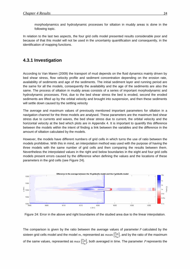
amount of siltation calculated by the models.
However, the models have different numbers of grid cells in which turns the use of ratio between the
models prohibitive. With this in mind, an interpolation method was used with the purpose of having the
three models with the same number of grid cells and then comparing the results between them.
Nevertheless the interpolated values in the right and below boundaries in the eight and four grid cells
models present errors caused by the difference when defining the values and the locations of these
parameters in the grid cells (see Figure 24).
Figure 24: Error in the above and right boundaries of the studied area due to the linear interpolation.
The comparison is given by the ratio between the average values of parameter calculated by the
sixteen grid cells model and the model , represented as {
}, and by the ratio of the maximum
of the same values, represented as {
}, both averaged in time. The parameter P represents the

Chapter 4 Results 25
maximum bed shear stress due to currents and waves, the bed shear stress due to currents, orbital
velocity or horizontal velocity nearby the bed. The plots comparing the average and maximum values
of these four parameters between the models are in Appendix 5. In these plots a special attention is
given to the values locate nearby and inside the channel and in the surf zone because at those
locations the important processes responsible for siltation occurs as wave breaking and cross shore
and along shore sediment transport.
In summary, the average and maximum values calculated for these four parameters by the eight grid
cells model and sixteen grid cells model are relatively similar. In contrast, the four grid cells model
presented much smaller values for these parameters in those locations. In the four grid cells, both
maximum and average values for the maximum bed shear stress due to currents and waves and the
orbital velocity are greatly underestimated. These two parameters are ten times smaller in some of
those locations in the four grid cells model in relation to the values in the six grid cells model. This
might have been caused by coarsening of the wave grid. Due to the wave forcing being poorly
computed, the erosion of the bed was underestimated and that explains the considerable small
amount of sediments computed by the four grid cells model observed in the sensitivity analysis.
4.4 Selecting uncertainty quantification method The LHS is chosen to quantify the uncertainty in the output. The idea is to use LHS subsamples from
the original LHS sample due to the expensive computational time required by the eight grid cells
model and the sixteen grid cells model. The original sample has 80 samples in which 40 samples are
chosen, and from this subsample, 20 samples are chosen to the end that the three models have a
common sample space.
The original sample is represented by a matrix with 80 rows and 3 columns. Each row consists of
three different cumulative probabilities values for the three parameters sampled by the LHS method.
The first, second and third columns correspond to the sampled cumulative probabilities of the bed
roughness, settling velocity and significant wave height distributions, respectively. For the bed
roughness and settling velocity a normal probabilistic distribution are assumed and for the wave
height a generalized extreme value probabilistic distribution is chosen to be valid (see Figure 25).
Figure 25: Generalized Extreme Value distribution fit.
Looking carefully at Figure 26, it can be noticed that each column and each line have one value. That is to say, that both settling velocity and bed roughness distributions before divided into 80 parts with equally probability are sampled. This plot is a 2D-LHS sampling arrangement for two of the three parameters. The other two 2D plots and a 3D plot can be found in Appendix 3. The next step after generating the 80 samples is to generate the 40 subsamples from the 80 samples and at last the 20 subsamples from the 40 samples.
av {𝝉
𝝉 }

Chapter 4 Results 26
Figure 26: The Latin hypercube arrangement of the original sampling points.
However, the computation of the 40 subsamples requires many days running in Matlab due to the
several possibilities of combination during the simulation for a 3D LHS. The number of combinations
are 80!/(40!(80-40)!) which is approximately 1.07 x 10²³
possible combinations. Due to the short time
available for this study, the best guess given by Matlab is adopted. Therefore, after 1.000.000
iterations the best guess was 37 samples within 40 strata. For each of the three dimensions three
strata are missing. In order to make sure that all the strata are sampled, eight samples from the 80
samples are added. In total there are 45 samples within 40 strata. Given that, there are strata which
are sampled more than once. The same problem happens when subsampling 20 samples from the 40
samples. In the end the best guess is 25 samples within 20 strata.
4.5 Uncertainty quantification
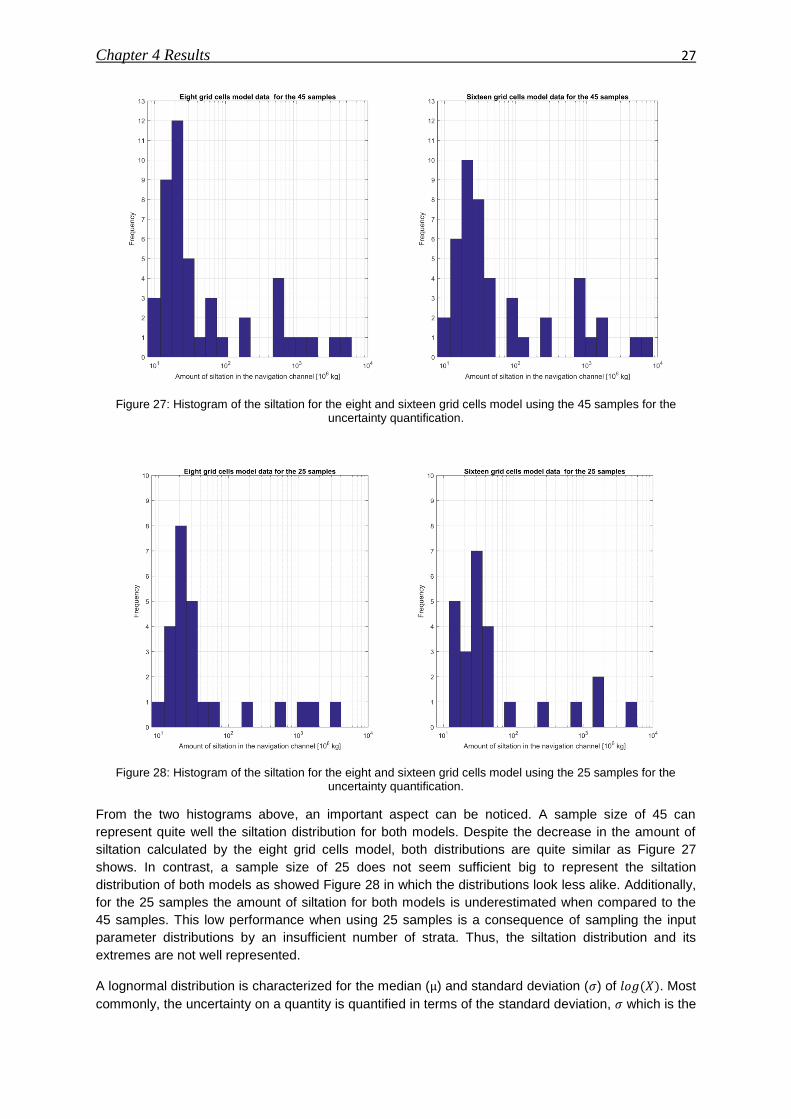
Among all the probability distribution functions (pdf’s), the lognormal was chosen to fit the distribution
of siltation in the navigation channel calculated by the three models using different sample sizes. A
random variable is said to be log-normally distributed if is normally distributed. In this case,
only positive values are possible and the distribution is skewed to the left. Skewed distributions are
characterized by low mean values, large variances and non-negative values. These characteristics
can be observed in Figure 27 and Figure 28. In addition, a chi-square goodness-of-fit test is applied
and it confirms that the data samples come from a lognormal distribution.
Chapter 4 Results 27
Figure 27: Histogram of the siltation for the eight and sixteen grid cells model using the 45 samples for the uncertainty quantification.
Figure 28: Histogram of the siltation for the eight and sixteen grid cells model using the 25 samples for the uncertainty quantification.
From the two histograms above, an important aspect can be noticed. A sample size of 45 can
represent quite well the siltation distribution for both models. Despite the decrease in the amount of
siltation calculated by the eight grid cells model, both distributions are quite similar as Figure 27
shows. In contrast, a sample size of 25 does not seem sufficient big to represent the siltation
distribution of both models as showed Figure 28 in which the distributions look less alike. Additionally,
for the 25 samples the amount of siltation for both models is underestimated when compared to the
45 samples. This low performance when using 25 samples is a consequence of sampling the input
parameter distributions by an insufficient number of strata. Thus, the siltation distribution and its
extremes are not well represented.
A lognormal distribution is characterized for the median ( ) and standard deviation ( ) of . Most
commonly, the uncertainty on a quantity is quantified in terms of the standard deviation, which is the

Chapter 4 Results 28
positive square root of variance, . In order to determine these values in terms of , the measure
data, the two formulations are used, where and are called the ‘back-
transformed’ values. Lognormal cumulative distribution functions (cdf’s) for the siltation computed by
the sixteen grid cells model and eight grid cells model using the 45 and 25 samples are found in
Figure 29 and Figure 30.
Figure 29: According to these cdf's, for the same probability the values of siltation computed by the eight grid cells model are smaller than by the sixteen grid cells model using the same 45 sample size. It can be observed that the difference in the amount of siltation between both models is small for the lower and higher percentiles.
However it increases considerably from the 60th to the 90
th percentiles. Thus, the extremes values are well
represented by the eight grid cells model.
Figure 30: According to these cdf's, for the same probability the values of siltation computed by the eight grid cells model are smaller than the sixteen grid cells model for the same 25 sample size. The difference in the
amount of siltation between both models is small for the lower percentiles, it increases considerably from the 60th
to the 90th percentiles and then it decreases again.

Chapter 4 Results 29
The differences in the cdf’s between both models showed in Figure 29 and Figure 30 are bigger for
the 25 samples than for the 45 samples. The legends in these figures show the ‘back-transformed’
median and standard deviations for both models. For the 45 samples, µ = 3.99 and σ 1.69 for the
eight grid cells model and µ = 4.20 and σ 1.78 for the sixteen grid cells model. For the 25 samples, µ
= 3.87 and σ 1.62 for the eight grid cells model and µ = 4.08 and σ = 1.71 for the sixteen grid cells
model.
Not only cumulative distribution are created with the purpose of uncertainty analysis, but also box
plots. In descriptive statistics, a boxplot is a convenient way of graphically illustrate groups of data
along their quartiles. On each box, the central mark indicates the median, and the bottom and top
edges of the box indicate the 25th and 75th percentiles, respectively. The lines extending vertically
from the boxes (whiskers) indicate variability outside the upper and lower quartiles. The outliers are
plotted as individual points. Box plots are non-parametric in which the variation in samples of a
statistical population is displayed without making any assumptions of the underlying statistical
distribution. The spacing between the different parts of the box indicates the degree of dispersion
(spread) and skewness in the data, and shows outliers.
Figure 31: New scatter plot and box plot combined for uncertainty analysis. From this plot, the box plot corresponding to the siltation data computed by the eight grid cells models is smaller than the box plot of the
sixteen grid cells model. The size of the box plot corresponds to the range of the measured data. The results of the eight grid cells model are not reliable.
The most important aspect of Figure 31 is the smallest amount of uncertainty in the siltation data computed by the eight grid cells model when compared to the sixteen grid cells model. The eight grid cells model gives a false idea of uncertainty in the siltation distribution. Therefore, the eight grid cells model is not reliable to be implemented in uncertainty quantification. It is also important to realize that the median calculated by the eight grid cells model is underestimated if compared to the median of the sixteen grid cells model for the same sample.

Chapter 4 Results 30
4.6 Identifying mapping function
In order to identify a mapping function from the eight grid cells moel to the sixteen grid cells model,
both distributions were plotted against each other and a polyline fit was applied as Figure 32 and
Figure 33 present. The aim of these polyline fits is to map the amount of siltation inside of the channel
from one model to the other. A fitting curve in a logarithm scale is chosen in order to better fit entire
the siltation data.
Figure 32: Experimental mapping function relating the amount of siltation calculated by the sixteen grid cells model and eight grid cells model with 45 samples. The plot shows that the logarithms of both siltation
distributions are related by a linear fit.
Figure 33: Experimental mapping function relating the amount of siltation calculated by the sixteen grid cell model and eight grid cells model with 25 samples. The plot shows that the logarithms of both siltation distributions are
related by a linear fit.

Chapter 4 Results 31
These two experimental mapping functions termed as and for the 25 samples and 45
samples, respectively, have a slope-intercept form where is the slope and is the
intercept. If the slope and the intercept are known, a linear relation between two variables can be
found.
Looking at the experimental mapping functions in Figure 32 and Figure 33, it can be observed that
both mapping functions have the same slope, but different intercepts. The logarithms of the siltation of
the two models have the same linear relationship for both samples as . While the intercept
of the mapping function is very small (close to zero), the intercept of the mapping function is
bigger which reduces the difference between the logarithms of both siltations. Thefore, when using 45
samples the values of siltation between the sixteen and eight grid cells models are closer than when
using 25 samples.
Regarding the lognormal mapping functions, two diagrams were created to show the results for the
two samples. The diagram for the 25 samples and the 45 samples can be found in Figure 34 and
Figure 35, respectively.
Figure 34: Diagram presenting the results for the 45 samples.
Figure 35: Diagram presenting the results for the 25 samples.
45
sam
ple
s
(µ)
8 grid cells model
4.19 x 1.05 3.99
16 grid cells model
45
sam
ple
s
(σ)
1.78 x 1.05 1.69
25
sam
ple
s
(µ)
8 grid cells model
4.08 x 1.05 3.87
16 grid cells model
25
sam
ple
s
(σ)
1.71 x 1.06 1.62

Chapter 4 Results 32
The values of the medians and standard deviations for the lognormal siltation distributions are inside
of the rectangles and the lognormal mapping functions and are the ratios above the
arrows. The consists of the ratios related to the median and standard deviation in Figure 34
and consists of the ratios in Figure 35. It can be noticed that these mapping functions are
almost the same for the two samples. For both models, the medians and standard deviations are
underestimated when using only 25 samples.
From the Uncertainty Quantification chapter, it was concluded that the eight grid cells model cannot
be used in uncertainty quantification because it is not a good representation of the expected range of
siltation that takes place in a navigation channel. It is worth investigating if the eight grid cells model
together with a mapping function can be used in uncertainty quantification. In addition, it is also
investigated the results when using a mapping function constructed from a 25 samples but using 45
samples. In that case, the advantages are determining a mapping function with part of the data and
using the other part for validation.
Firstly, the two experimental mapping functions found in Figure 32 and Figure 33 were applied to the
siltation data computed by the eight grid cells model for the 45 samples. The comparison between
these mapped siltation distributions and the siltation distribution calculated by the sixteen grid cell
model is showed in Figure 36.
Figure 36: Visual uncertainty quantification for the experimental mapped siltation distributions and the siltation distribution from the sixteen grid cells model using box plots.
In Figure 36, the first box plot and the red circles represent the siltation distribution computed by the
sixteen grid cells model, the second box plot and the blue pentagrams represent the experimental
mapped siltation for the and the third box plot and green diamonds represent the experimental
mapped siltation for the . After applying these mapping functions, the siltation distributions look
very alike. Besides the similar values of medians, the range represented by the size of the box plots
(including the whiskers) is approximately the same. Therefore, the eight grid cells model when
combined with one of the experimental mapping functions present results very similar to the six grid
cells model for uncertainty quantification.

Chapter 4 Results 33
Regarding the lognormal mapping functions, they are applied to 45 random numbers generated from
a lognormal distribution with µ=3.99 and σ=1.69 which are the parameters values for the eight grid
cells model siltation distribution, see Figure 34. Next, a comparison of uncertainty quantification
between these lognormal mapped siltation distributions and the siltation distribution computed by the
sixteen grid cells model is showed in Figure 37.
Figure 37: Visual uncertainty quantification for the lognormal mapped siltation distributions and the siltation distribution from the sixteen grid cells model using box plots.
The first box plot and the red circles represent the siltation distribution computed by the sixteen grid
cells model, the second box plot and the blue pentagrams represent the mapped siltation for
and the third box plot and green diamonds represent the mapped siltation for . Within this plot,
two important aspects need to be highlighted. Firstly, the medians of the mapped siltation distributions
are greatly overestimated as a consequence of the lognormal distribution fit. Secondly, mapped
siltation distributions have a larger amount of uncertainty than in the siltation from the sixteen grid cell
models. Therefore, fitting lognormal distribution to siltation data do not give correct results that can be
used for uncertainty quantification.

34
_________________________________________________________________________________________________
5 Discussion
____________________________________________________________________________________________________
A Delft3D model and two emulators were used to quantify the amount of uncertainty in the siltation
distribution. The results are compared and mapping functions are applied in order to translate the
amount of uncertainty in the model output from the emulator output. Here some points about the
limitations and assumptions of this study are discussed:
1. In this study, some of the assumptions made as no wind effect, perpendicular approach of the
waves to the coast and low discharge had a big impact on the sensitivity analysis in which the
most sensitive uncertain parameters presented to be the settling velocity, bed roughness and
significant wave height. In case these assumptions are not made, the outcome of the
sensitivity analysis might be different;
2. This study is very case specific due to the assumptions and parameters intervals adopted.
Due to that, the results of this study are quite limited. However, the methodology here applied
in uncertainty quantification using an emulator can also be implemented in other studies;
3. The LHS method shows to be a good sampling method as long as the sample size is not very
small. A sample size of 25 showed to give results less accurate than the 45 samples.
4. The lognormal probability density function fits the siltation distribution from the sixteen and
eight grid cells model, nonetheless it has the disadvantage of increasing its median value;

35
_____________________________________________________________________________________________________
6 Conclusion _____________________________________________________________________________________________________
Let’s hightlight three important conclusions from this study. First, the eight grid cells model is a good
replacement for the sixteen grid cells model with respect to siltation computation in the navigation
channel. Second, the four grid cells model can be used for a ‘parameter screening’ in sensitivity
analysis. Third, the eight grid cell model can be used for uncertainty quantification if the specified
mapping functis are applied. Summarizing, it is possible to quantify the uncertainty in a navigation
channel using an emulator as long as a mapping function is applied. With attention to the fact that the
channel width should be around 10 grid cells, otherwise the hydrodynamics and morphodynamics are
not well represented by the emulator. Equally important, the research questions presented in
Introduction can now be answered.
1. What are the uncertain input parameters with respect to a coastal morphodynamic
model?
For a coastal morphodynamic model which the study area is characterized by low wind
velocities, waves coming from deep sea and a river discharge, the uncertain input parameters
will be river discharge, critical shear stress for erosion, settling velocity, bed roughness and
significant wave height.
2. What are the most sensitive uncertain input parameters for a Delft3D model?
For both model and emulators, the most sensitivity parameters are the settling velocity, wave
height and the bed roughness. Although the discharge is an important parameter, because it
brings sediments into the system, it was found to not be relevant in this study due to its low
values.
3. In what way do the uncertain in the siltation between model and emulators differ
between them?
The siltation distribution computed by the eight grid cells model presented much less
uncertainty when compared to the siltation distribution computed by sixteen grid cells model.
However, this is not a realistic result. Given that, the eight grid cells underestimate the real
range of the siltation distribution. The four grid cells model does not correctly compute the
hydrodynamics and morphodynamics due to its coarse grid, thus it was not applied in
uncertainty quantification.
4. Can a mapping function be applied to the emulators in order to map the amount of
uncertainty in the siltation distribution computed by the model?
For this study, the relation between the siltation computed by the sixteen grid cells model and
eight grid cells models is log linear. The experimental mapping functions are
and where is the
siltation data calculated by the eight grid cells model and is the mapped siltation. If these
mapping functions are applied to the eight grid cells model data, then this model can be used
in uncertainty quantification. The lognormal mapping functions do not present good results in
uncertainty quantification.

36
_____________________________________________________________________________________________________
7 Recommendation _____________________________________________________________________________________________________
This study used a Delft3D model and two emulators in order to calculate the amount of uncertainty in port siltation. Within the known assumptions and conditions of this study, some recommendations can be done:
For ‘screening parameter’, or qualitative sensitivity analysis, is recommended to use a coarse emulator instead of a model, because it will give the same result in a much short period of time.
For uncertainty quantification, an emulator can be used as long as it has around 10 grid cells
along the channel width and whether there is a mapping function capable to map the siltation
distribution of this emulator to its model. If that is not the case, the model should be used in
uncertainty quantification. Because the emulator without a mapping function gives a siltation
distribution in which the amount of uncertainty is underestimated may causing future losses to
the client;
In order to build mapping functions, few data points are necessary. In future works in which is
desired to determine the amount of uncertainty in port siltation using an emulator, part of the
data calculated by the model can be reserved to build a mapping function while the other part
to validate it. For a emulator which has around 10 grid cells along the navigation channel and
the most sensitivite parameters are the settling velocity, wave height and bed roughness, the
experimental mapping function can be applied for uncertainty analysis
using 45 LHS samples;
For future works, it may be worth to investigate until what sample size the mapping function
can be improved. Here, the mapping function from the 45 samples fits better the data than the
25 samples. It is expected that this improvement of the mapping function reaches its limits
due to the own limitation of the emulator;
The possibility of using an emulator with a mapping function brings the possibility of making
this case specific into a more general case. Given that, other uncertain input parameters and/
or wider parameter ranges can be adopted in order to verify the existence of a mapping
function which together with an emulator could be applied in several projects. Thus, a applied
research institute as Deltares would be able to give in a short period of time the feasibility of
building a port in a certain area based on the uncertainty quantification done by an emulator
together with this more general mapping function.

37
_____________________________________________________________________________________________________
References ____________________________________________________________________________________________________
Baveye, P., Myslak, J. & Laba, M., 2007. Uncertainties in Environmental Modelling and Consequences
for Policy Making. Vrsar, Croatia, Springer.
Becker, S., Holmes, R., Maly, T. & Milligan, B., 2013. Dredge. [Online] Available at:
http://dredgeresearchcollaborative.org/works/dredge/ [Accessed 10 July 2016].
Beven, K., 2009. Environmental Modelling: An Uncertain Future?. 1st ed. New York, USA: Routledge.
Brown, J. & Bearman, G., 1999. Waves, Tides & Shallow-Water Processes. Oxford: Open University.
Cambridge, U., 2016. Cambridge Advanced Learner’s Dictionary & Thesaurus. [Online] Available at:
http://dictionary.cambridge.org/dictionary/english/uncertainty
Castelleti, A. et al., 2012. A general framework for Dynamic Emulation Modelling in environmental
problems.. pp. 5-18.
Chang, C., Yang, J. & Tung, Y., 1993. Sensitivity and uncertainty analysis of a sediment transport
model: a global approach.. December, Volume 7, pp. 299-314.
Christiaens, K. & Feyen, J., 2001. Analysis of uncertainties associated with different methods to
determine soil hydraulic properties and their propagation in the distributed hydrological MIKE SHE
model.. Journal of Hydrology, 1(246), pp. 63-81.
Cooke, R. M. & Slijkhuis, K. A., 2002. Expert Judgment in the Uncertainty Analysis of Dike Ring Failure
Frequency. In: Case Studies in Reliability and Maintenance. NJ: John Wiley & Sons.
Deltares, 2011. Sedimentation in channels and ports. [Online] Available at: www.deltares.nl
Deltares, 2014. Delft3D-FLOW User Manual. Delft: Deltares.
Fortunate, A., Bertin, X. & Oliveira, A., 2009. Space and time variability of uncertainty in
morphodynamic simulations. Costal Engineering, Volume 56, pp. 886-894.
Hamby, D. M., 1994. A review of techniques for parameter sensitivity analysis of environmental
models. Environmental Monitoring and Assessment, September, 32(2), pp. pp 135-154.
Koziel, S. & Bandler, J. W., 2008. Space Mapping With Multiple Coarse Models for Optimization of
Microwave Components. IEEE Microwave and Wireless Components Letters , January.18(1).
Kuang, C. P. & Chen, W., 2014. Comprehensive analysis on the sediment siltation in the upper reach
of the deep-water navigation channel in the Yangtze Estuary.. Journal of Hydrodynamics.
Loucks, D. P. & van Beek, E., 2005. Water Resources Systems Planning and Management. Delft, The
Netherlands: UNESCO.

Chapter References 38
Maren, B. v., n.d. An introduction to cohesive sediment transport modelling. s.l., s.n.
McKay, M., Beckman, R. & Conover, W., 1979. A Comparison of Three Methods for Selecting Values
of Input Variables in the Analysis of Output from a Computer Code. Technometrics, May, 21((2)), pp.
239-245.
Morgan, C. S. & Henrion, M., 1990. Uncertainty. A guide to dealing with uncertainty in quantitative
risk and policy analysis.. Cambridge: Cambridge Unversity Press.
Morgan, M. G. & Keith, D. W., 1995. Subjective Judgments by Cilmate Experts. 29(10).
Plüß, A. & Kösters, F., 2014. Morphodynamic modelling for the entire German Bight: an initial study
on model sensitivity and uncertainty. EGU Journal.
Roelvink D., R. A., 2010. Coastal Morphology Modeling Guide. s.l.:World Scientific Book.
Roelvink, D. J. A. & Walstra, D., 2005. Keeping it simple by using complex models. Advances in Hydro-
Science and -Engineering, Volume 6, pp. 1-11.
Saltelli, A., 1999. Sensitivity analysis: Could better methods be used?. 20 February, Volume 104, pp.
3789-3793.
Saltelli, A., Chan, K. & Scott, M., 2000. Sensitivity Analysis. New York, USA: Wiley.
Scheel, F. et al., 2014. On the Generic Utilization of Probabilistic Methods for Quantification of
Uncertainty in Process-Based Morphodynamic Model Applications. Delft, The Netherlands, Coastal
Engineering Research Council.
Soulsby, R. L. et al., 1993. Wave-current interaction within and outside the bottom boundary layer.
Coastal Engineering, December, Volume 21, pp. 41-69.
Van der Klis, H., 2003. Uncertainty Analysis applied to Numerical Moels of River Bed Morphology.
Delft: DUP Science.
Van Maren, B., 2009. Background theory cohesive-fine sediment-mud. [Online] Available at:
http://oss.deltares.nl/web/delft3d/community-
wiki;jsessionid=20D4C18A12047739F9C2253F2FE5E42A.v-
oss002.dlt.proteon.nl?p_p_id=36&p_p_lifecycle=0&p_p_state=normal&p_p_mode=view&p_p_col_i
d=column-1&p_p_col_count=1&_36_struts_action=%2Fwiki%2Fview_page_attach
[Accessed 10 July 2016].
Van Rijn, L., 2013. [Online] Available at: www.leovanrijn-sediment.com
Van Rijn, L. C., 2005. Estuarine and Coastal Sedimentation Problems. Volume 20.
Vollmers, H. J., 1989. The state of Art of Physical Modelling of Sediment Transport. s.l., American
Society of Civil Engineering, pp. 7-12.
Walker, W. E. et al., 2003. Defining Uncertainty: A Conceptual Basis for Uncertainty Management in
Model-Based Decision Support.. Issue 4, pp. 5-17.

Chapter References 39
Wikipedia, 2016. Sensitivity Analysis. [Online]
Available at: https://en.wikipedia.org/wiki/Sensitivity_analysis [Accessed 2016 July 16].
Winterwerp, J. C. V. K. W. G. M., 2004. Introduction to the physics of cohesive sediment dynamics in
the marine environment. Developments in Sedimentology. Amsterdam: Elsevier.
Yeah, K. -C. & Tung, Y. -K., 1993. Uncertainty and sensitivity analyses of pit-migration model. Journal
of Hydraulic Engineering, 2(119), pp. 262-283.

40
_____________________________________________________________________________________________________
Appendix 1: Subjective sensitivity _______________________________________________________________________________________________________________________________________________________
Table 5: Delft3D-FLOW input parameters.
Delft3D-FLOW
Input paramete
r Variable Uncertain Comment Unit
Initial conditions
Water level N Do not have a big influence on the system analysed. m
Salinity N Determined in the model set-up. ppt
Sediment concentration N Determined in the model set-up. Kgm-3
Boundaries
Offshore N Constant m
River discharge Y
Due to prediction uncertainty in precipitation, run-off and evaporation in the river watershed. m
3s
-1
Neumann-north N Constant m
Neumann-south N Constant m
Physical Paramete
rs
Gravity N Constant ms-2
Water density N Constant kgm-3
Temperature N Constant ⁰C
Horizontal eddy viscosity N Calibration parameters. m2s
-1
Horizontal eddy diffusity N Calibration parameters. m2s
-1
Vertical eddy viscosity x Not considered in the model. m2s
-1
Vertical eddy diffusivity x Not considered in the model. m2s
-1
Ozmidov length scale x Not considered in the model. m
Specific density Y Depends on the mineral composition kgm-3
Dry bed density Y It will not change due to short run period. kgm-3
Fresh settling velocity Y It will affect the cohesive sediment settling velocity. mms-1
Saline settling velocity Y It will affect the cohesive sediment settling velocity. mms-1
Hindered settling velocity N Significant for multiple suspended sediment fractions. mms-1
Critical bed shear stress for erosion Y Uncertain parameter. Nm
-2
Erosion Parameter N It is assumed to be constant. Salinity for saline velocity N It is assumed to be constant. ppt
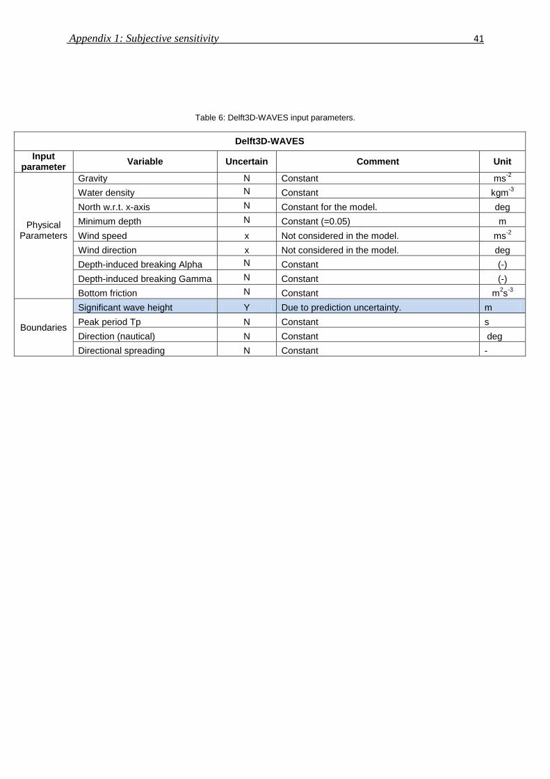
Appendix 1: Subjective sensitivity 41
Table 6: Delft3D-WAVES input parameters.
Delft3D-WAVES
Input parameter
Variable Uncertain Comment Unit
Physical Parameters
Gravity N Constant ms-2
Water density N Constant kgm-3
North w.r.t. x-axis N Constant for the model. deg
Minimum depth N Constant (=0.05) m
Wind speed x Not considered in the model. ms-2
Wind direction x Not considered in the model. deg
Depth-induced breaking Alpha N Constant (-)
Depth-induced breaking Gamma N Constant (-)
Bottom friction N Constant m2s
-3
Boundaries
Significant wave height Y Due to prediction uncertainty. m
Peak period Tp N Constant s
Direction (nautical) N Constant deg
Directional spreading N Constant -

42
____________________________________________________________________________________________________________________________________________________________
Appendix 2: Sensitivity analysis ____________________________________________________________________________________________________________________________________________________________
:
Table 7: Resolution factors and amount of siltation in the navigation channel.
Models Reference (P50)
Bed roughness Critical S. S. for Erosion Discharge Settling Velocity Significant Wave Height
P10 (kg) P90 (kg) P10 (kg) P90 (kg) P10 (kg) P90 (kg)
P10 (kg) P90 (kg)
P10 (kg) P90 (kg)
16GRID 335.713.900,0 24.932.176 1.501.509.900 65.402.409 762.833.910 135.702.090 1.056.635.000 101.580.570 1.612.810.000 18.235.234 1.476.567.400
Fr16,8 1,.5 1.4 1.4 1.4 1.4 1.3 1.6 1.4 1.5 1.1 1.4
8GRID 230.746.620,0 17.620.665 1.070.783.500 46.513.312 559.353.780 106.119.760 670.044.680 74.616.003 1.108.763.000 17.050.050 1.035.352.900
Fr8,4 3.7 1.9 2.8 2.9 3.0 2.6 4.2 3.6 3.0 1.7 2.6
4GRID 62.921.560,0 9.227.299,5 380.390.730 16.246.230 187.632.560 41.309.384 158.449.450 20.773.887 370.027.630 9.919.559 391.620.060
Fr16,4 5.3 2.7 4.0 4.0 4.1 3.3 6.7 4.9 4.4 1.8 3.8
Table 8: Parameter factors and amount of siltation in the navigation channel.
odels Bed roughness (n)
Critical S. S. for Erosion
( Discharge Settling Velocity Significant Wave Height
P10 (kg) P90 (kg) P10 (kg) P90 (kg) P10 (kg) P90 (kg) P10 (kg) P90 (kg) P10 (kg) P90 (kg)
16GRID 24.932.176 1.501.509.900 65.402.409 762.833.910 135.702.090 1.056.635.000 101.580.570 1.612.810.000 18.235.234 1.476.567.400
60.2 11,7 7,8 15,9 81.0
8GRID 17.620.665 1.070.783.500 46.513.312 559.353.780 106.119.760 670.044.680 74.616.003 1.108.763.000 17.050.050 1.035.352.900
60.8 12,0 6,3 14.9 60.7
4GRID 9.227.299,50 380.390.730 16.246.230 187.632.560 41.309.384 158.449.450 20.773.887 370.027.630 9.919.559 391.620.060
41.2 11.5 3.8 17.8 39.5

43
____________________________________________________________________________________________________________________________________________________________
Appendix 3: Latin Hypercube samples _______________________________________________________________________________________________________________________________________________________________________________
Figure 38: 3-Dimensional LHS’s (80 strata).

Appendix 3: Latin Hypercube samples 44
Figure 39: 2-Dimensional LHS’s (80 strata).

Appendix 3: Latin Hypercube samples 45
Figure 40: 2-Dimensional LHS' sample (80 strata).

Appendix 3: Latin Hypercube samples 46
Figure 41: 2-Dimensional LHS' sample (80 strata).

Appendix 3: Latin Hypercube samples 47
Figure 42: 3-Dimensional LHS’s (40 strata)

Appendix 3: Latin Hypercube samples 48
Figure 43: 2-Dimensional LHS' sample (40 strata).

Appendix 3: Latin Hypercube samples 49
Figure 44: 2-Dimensional LHS' sample (40 strata).

Appendix 3: Latin Hypercube samples 50
Figure 45: 2-Dimensional LHS' sample (40 strata).

Appendix 3: Latin Hypercube samples 51
Figure 46: 3-Dimensional LHS' sample (20 strata).
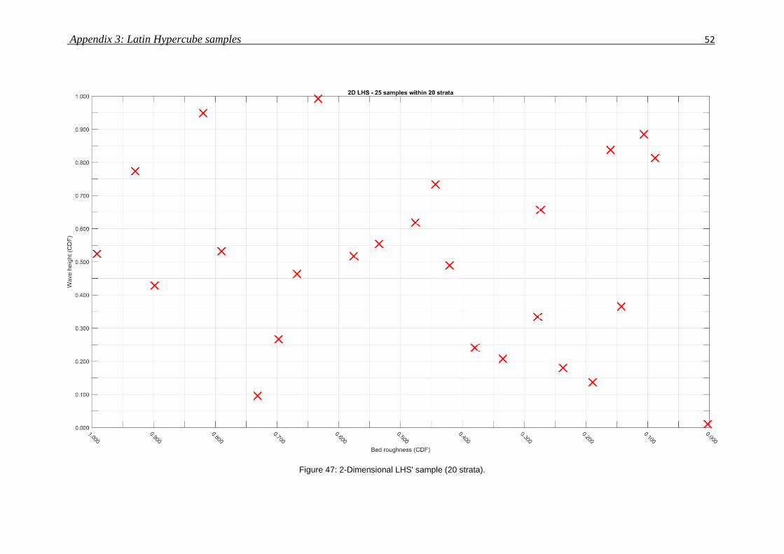
Appendix 3: Latin Hypercube samples 52
Figure 47: 2-Dimensional LHS' sample (20 strata).

Appendix 3: Latin Hypercube samples 53
Figure 48: 2-Dimensional LHS' sample (20 strata).

Appendix 3: Latin Hypercube samples 54
Figure 49: 2-Dimensional LHS' sample (20 strata).

55
__________________________________________________________________________________
Appendix 4: Investigation of the maximum bed shear
stress due to currents and waves, the bed shear stress due
to currents, the orbital velocity and the horizontal velocity
at the bed _____________________________________________________________________________________________________
Figure 50: Median values of the maximum bed shear stress averaged in time computed by the 16 grid cells model.
Figure 51: Median values of the maximum bed shear stress averaged computed by the 8 grid cells models.
Figure 52: Median values of the maximum bed shear stress averaged in time computed by the 4 grid cells model.
.

Appendix 4: Investigation of the maximum bed shear stress due to currents and waves, the
bed shear stress due to currents, the orbital velocity and the horizontal velocity at the bed 56
Figure 53: Highest values for the maximum bed shear stress averaged in time computed by the 16 grid cells model
Figure 54: Highest values for the maximum bed shear stress averaged in time computed by the 8 grid cells model.
Figure 55: Highest values for the maximum bed shear stress averaged in time computed by the 4 grid cells model.
Figure 56: Median values for the bed shear stress averaged in time computed by the 16 grid cells model.
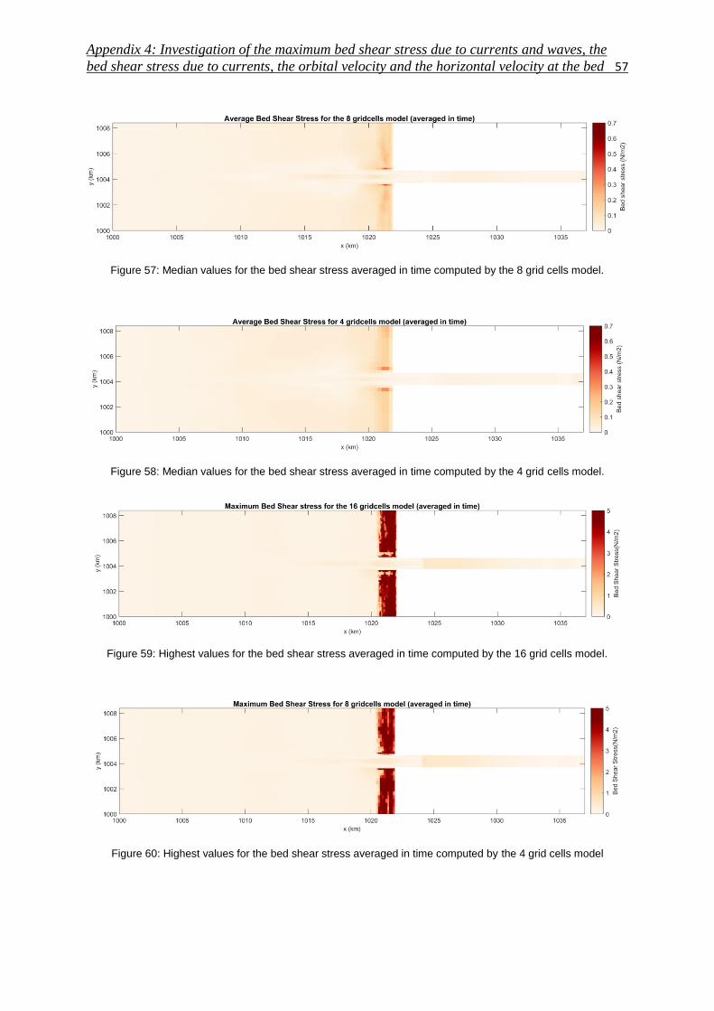
Appendix 4: Investigation of the maximum bed shear stress due to currents and waves, the
bed shear stress due to currents, the orbital velocity and the horizontal velocity at the bed 57
Figure 57: Median values for the bed shear stress averaged in time computed by the 8 grid cells model.
Figure 58: Median values for the bed shear stress averaged in time computed by the 4 grid cells model.
Figure 59: Highest values for the bed shear stress averaged in time computed by the 16 grid cells model.
Figure 60: Highest values for the bed shear stress averaged in time computed by the 4 grid cells model

Appendix 4: Investigation of the maximum bed shear stress due to currents and waves, the
bed shear stress due to currents, the orbital velocity and the horizontal velocity at the bed 58
Figure 61: Median values for the bed shear stress averaged in time computed by the 4 grid cells model.
Figure 62: Median values for the orbital velocity averaged in time computed by the 16 grid cells model.
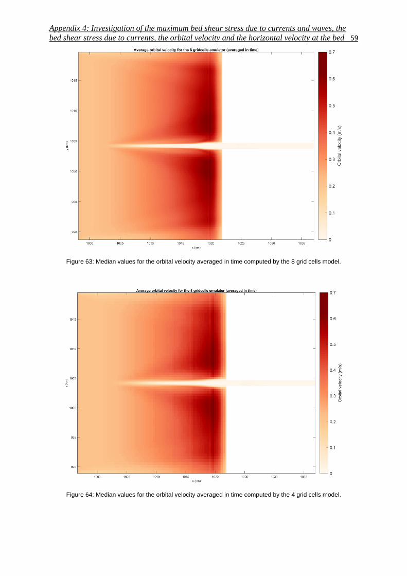
Appendix 4: Investigation of the maximum bed shear stress due to currents and waves, the
bed shear stress due to currents, the orbital velocity and the horizontal velocity at the bed 59
Figure 63: Median values for the orbital velocity averaged in time computed by the 8 grid cells model.
Figure 64: Median values for the orbital velocity averaged in time computed by the 4 grid cells model.

Appendix 4: Investigation of the maximum bed shear stress due to currents and waves, the
bed shear stress due to currents, the orbital velocity and the horizontal velocity at the bed 60
Figure 65: Highest values for the orbital velocity averaged in time computed by the 16 grid cells model.
Figure 66: Highest values for the orbital velocity averaged in time computed by the 8 grid cells model.

Appendix 4: Investigation of the maximum bed shear stress due to currents and waves, the
bed shear stress due to currents, the orbital velocity and the horizontal velocity at the bed 61
Figure 67: Highest values for the orbital velocity averaged in time computed by the 4 grid cells model.
Figure 68: Median values for the horizontal velocity at the bed averaged in time computed by the 16 grid cells model.
Figure 69: Median values for the horizontal velocity at the bed averaged in time computed by the 8 grid cells
model.

Appendix 4: Investigation of the maximum bed shear stress due to currents and waves, the
bed shear stress due to currents, the orbital velocity and the horizontal velocity at the bed 62
Figure 70: Median values for the horizontal velocity at the bed averaged in time computed by the 8 grid cells
model.
Figure 71: Highest values for the horizontal velocity at the bed averaged in time computed by the 4 grid cells model.
Figure 72: Highest values for the horizontal velocity at the bed averaged in time computed by the 4 grid cells model.
Figure 73: Highest values for the horizontal velocity at the bed averaged in time computed by the 4 grid cells model.

63
_____________________________________________________________________________________________________
Appendix 5: Comparison between maximum bed shear
stress due to currents and waves, bed shear stress due to
currents, orbital velocity and horizontal velocity at the bed ____________________________________________________________________________________________________
Figure 74: Ratio of the average values maximum bed shear stress between the 16 and 8 grid cells model.
Figure 75: Ratio of average values of the maximum bed shear stress between the 16 and 4 grid cells model.
Figure 76: Ratio of maximum values of the maximum bed shear stress between the 16 and 8 grid cells model.
mean {𝝉
𝝉 }
mean {𝝉
𝝉 }
max {𝝉
𝝉 }

Appendix 5: Comparison between maximum bed shear stress due to currents and waves, bed
shear stress due to currents, orbital velocity and horizontal velocity at the bed 64
Figure 77: Ratio of maximum values of the maximum bed shear stress between the 16 and 4 grid cells model.
Figure 78: Ratio of average values of the bed shear stress between the 16 and 8 grid cells model.
Figure 79: Ratio of average values of the bed shear stress between the 16 and 4 grid cells mode
mean {𝝉
𝝉 }
mean {𝝉
𝝉 }
max {𝝉
𝝉 }

Appendix 5: Comparison between maximum bed shear stress due to currents and waves, bed
shear stress due to currents, orbital velocity and horizontal velocity at the bed 65
Figure 80: Ratio of maximum values of the bed shear stress between the 16 and 8 grid cells model.
Figure 81: Ratio of maximum values of the bed shear stress between the 16 and 4 grid cells model.
Figure 82: Ratio of the average values of the orbital velocity of the 16 and 8 grid cells model.
max {𝝉
𝝉 }
max {𝝉
𝝉 }
mean {
}

Appendix 5: Comparison between maximum bed shear stress due to currents and waves, bed
shear stress due to currents, orbital velocity and horizontal velocity at the bed 66
Figure 83: Ratio of the average values of the orbital velocity of the 16 and 4 grid cells model.
Figure 84: Ratio of the maximum values of the orbital velocity of the 16 and 8 grid cells model.
mean {
}
max {
}

Appendix 5: Comparison between maximum bed shear stress due to currents and waves, bed
shear stress due to currents, orbital velocity and horizontal velocity at the bed 67
Figure 85: Ratio of the maximum values of the orbital velocity of the 16 and 4 grid cells model.
Figure 86: Ratio of the average values of the horizontal velocity at the bed of the 16 and 8 grid cells model.
Figure 87: Ratio of the average values of the horizontal velocity at the bed of the 16 and 4 grid cells model.
max {
}
a𝐯 {
}
{
}
a𝐯 {
}
{
}

Appendix 5: Comparison between maximum bed shear stress due to currents and waves, bed
shear stress due to currents, orbital velocity and horizontal velocity at the bed 68
Figure 88: Ratio of the maximum values of the horizontal velocity at the bed of the 16 and 4 grid cells model.
Figure 89: Ratio of the maximum values of the horizontal velocity at the bed of the 16 and 8 grid cells model.
max {
}
max {
}