ludwigs-maximilians-universitat˜ m˜unchen …€¦ · ludwigs-maximilians-universitat˜ m˜unchen...
TRANSCRIPT

Ludwigs-Maximilians-Universitat Munchen
— Departement for Physics —
University Observatory
Computational Methods in Astrophysics
Monte Carlo Simulationsand
Radiative Transfer
first edition (2005)
Joachim Puls
winter semester 2005/2006

ii

Contents
0 Introduction 1
1 Theory 1-11.1 Some basic definitions and facts . . . . . . . . . . . . . . . . . . . . . . . . . . . . 1-1
1.1.1 The concept of probability . . . . . . . . . . . . . . . . . . . . . . . . . . . 1-11.1.2 Random variables und related functions . . . . . . . . . . . . . . . . . . . 1-11.1.3 Continuous random variables . . . . . . . . . . . . . . . . . . . . . . . . . 1-2
1.2 Some random remarks about random numbers . . . . . . . . . . . . . . . . . . . 1-61.2.1 (Multiplicative) linear congruential RNGs . . . . . . . . . . . . . . . . . . 1-61.2.2 The minimum-standard RNG . . . . . . . . . . . . . . . . . . . . . . . . . 1-81.2.3 Tests of RNGs . . . . . . . . . . . . . . . . . . . . . . . . . . . . . . . . . 1-10
1.3 Monte Carlo integration . . . . . . . . . . . . . . . . . . . . . . . . . . . . . . . . 1-181.3.1 Preparation . . . . . . . . . . . . . . . . . . . . . . . . . . . . . . . . . . . 1-181.3.2 The method . . . . . . . . . . . . . . . . . . . . . . . . . . . . . . . . . . . 1-191.3.3 When shall we use the Monte Carlo integration? . . . . . . . . . . . . . . 1-221.3.4 Complex boundaries: “hit or miss” . . . . . . . . . . . . . . . . . . . . . . 1-231.3.5 Advanced reading: Variance reduction – Importance sampling . . . . . . . 1-24
1.4 Monte Carlo simulations . . . . . . . . . . . . . . . . . . . . . . . . . . . . . . . . 1-261.4.1 Basic philosophy and a first example . . . . . . . . . . . . . . . . . . . . . 1-261.4.2 Variates with arbitrary distribution . . . . . . . . . . . . . . . . . . . . . . 1-29
2 Praxis: Monte Carlo simulations and radiative transfer 2-12.1 Exercise 1: Simple RNGs and graphical tests . . . . . . . . . . . . . . . . . . . . 2-12.2 Exercise 2: Monte Carlo integration - the planck-function . . . . . . . . . . . . 2-22.3 Exercise 3: Monte Carlo simulation - limb darkening in stellar atmospheres . . . 2-3
iii

CONTENTS
iv

Chapter 0
Introduction
This part of our practical course in computational techniques deals with Monte Carlo meth-ods, which allow to solve mathematical/scientific/economic problems using random numbers.The essential approach is to approximate theoretical expectation values by averages over suit-able samples. The fluctuations of these averages induce statistical variances which have to beaccounted for in the analysis of the results. Most interestingly, Monte Carlo methods can beapplied for both stochastic and deterministic problems.
Some typical areas of application comprise
• statistics (tests of hypothesis, parameter estimation)
• optimization
• integration, particularly in high dimensions
• differential equations
• physical processes.
An inevitable prerequesite for this approch is the availability of a (reliable) random number gen-erator (RNG). Moreover, all results have to be analyzed and interpreted by statistical methods.
Outline. The outline of this manual is as follows. In the next chapter we will give an overviewof the underlying theoretical concept. At first we will summarize few definitions and facts regard-ing probabilistic approaches (Sect. 1.1). In Sect. 1.2 we will consider the “construction” of simpleRNGs and provide some possibilities to test them. An important application of Monte Carlotechniques constitutes the Monte Carlo integration which is presented in Sect. 1.3. The theoret-ical section is closed by an introduction into Monte Carlo simulations themselves (Sect. 1.4).
In Chap 2 we will outline the specific exercises to be solved during this practical work,culminating in the solution of one (rather simple) astrophysical radiative transfer problem bymeans of a Monte Carlo simulation.
Plan. The plan to carry out this part of our computational course is as follows: Prepare yourwork by carefully reading the theoretical part of this manual. If you are a beginner in MonteCarlo techniques, you might leave out those sections denoted by “advanced reading” (whichconsider certain topics which might be helpful for future applications).
1

CHAPTER 0. INTRODUCTION
On the first day of the lab-work then, exercise 1 and 2 should be finished, whereas the secondday covers exercise 3. Please have a look into these exercises before you will accomplish them, inorder to allow for an appropriate preparation.
Don’t forget to include all programs, plots etc. into your final elaboration.
2

Chapter 1
Theory
1.1 Some basic definitions and facts
1.1.1 The concept of probability
Let’s assume that we are performing an experiment, which can result in a number of differentand discrete outcomes (events), e.g., rolling a dice. These events shall be denoted by Ek, wherethe probability for the occurence of such an event,
P (Ek) = pk,
must satisfy the following constraints:
(a) 0 ≤ pk ≤ 1.
(b) If Ek cannot be realized, then pk = 0.If Ek is the definite outcome, then pk = 1.
(c) If two events, Ei and Ej , are mutually exclusive, then
P (Ei and Ej) = 0, P (Ei or Ej) = pi + pj .
(d) If there are N mutually exclusive events, Ei, i = 1, . . . , N , and these events are completeconcerning all possible outcomes of the experiment, then
N∑
i=1
pi = 1. (1.1)
For a two-stage experiment with events Fi and Gj , Eij is called the combined event (Gj hasoccured after Fi). If Fi and Gj are independent of each other, the probability for the combinedevent is given by
p(Eij) = pij = p(Gj) · p(Fi), (1.2)
1.1.2 Random variables und related functions
We now associate each discrete event, Ei, with a real number xi, called random variable (r.v.)or variate . E.g., the event E6 that the result of throwing a dice is a “six” might be associatedwith the r.v. x6 = 6. Of course, any other association, e.g., x6 = 1, is allowed as well.
1-1

CHAPTER 1. THEORY
The expectation value of a random variable (sometimes sloppyly denoted by “average” or“mean” value) is defined by
E(x) = x =
N∑
i=1
xipi, (1.3)
if the events Ei, i = 1, . . . , N are complete and mutually exclusive. Any arbitrary function ofthis random variable, g(x), is also a random variable, and we can construct the correspondingexpectation value,
E(g(x)) = g =N∑
i=1
g(xi)pi. (1.4)
Note that the expectation value is a linear operator,
E(ag(x) + bh(x)) = aE(g) + bE(h). (1.5)
The variance of a r.v.,
Var (x) = (x− x)2 = x2 − 2x · x + x2 = x2 − x2, (1.6)
describes the “mean quadratic deviation from the mean”, and
The standard deviation, σ, is defined as
σ(x) = (Var (x))1/2
.
In contrast to the expectation value, the variance is no linear operator (prove by yourself!).If g and h are statistically independent, i.e.,
gh = E(gh) = E(g) · E(h) = g · h,
one can show thatVar (ag + bh) = a2Var (g) + b2Var (h) . (1.7)
Thus, the standard deviation has the following scaling property,
σ(ag) = aσ(g).
1.1.3 Continuous random variables
So far, we have considered only discrete events, Ei, with associated discrete random variables,xi. How do we have to proceed in those cases where different events can be no longer enumerated(example: scattering angles in a scattering experiment)?
The probability for a distinct event (e.g., that an exactly specified scattering angle will be real-ized) is zero; on the other hand, the probability that the event lies inside a specific (infinitesimal)interval is well defined,
P (x ≤ x′ ≤ x + dx) = f(x)dx, (1.8)
where f(x) is the so-called probability density function (pdf).The probability that the result of the experiment will lie inside an interval [a, b] can be
calculated from this pdf,
P (a ≤ x ≤ b) =
b∫
a
f(x′)dx′. (1.9)
1-2

CHAPTER 1. THEORY
In analogy to the discrete probabilities, pi, also the pdf has to satisfy certain constraints:
(a) f(x) ≥ 0, −∞ < x <∞ (1.10a)
(b)
∞∫
−∞
f(x′)dx′ = 1 : (1.10b)
the combined probability that all possible values of x will be realized is unity!
The cumulative probability distribution (cdf), F (x), denotes the probability that all events upto a certain threshold, x, will be realized,
P (x′ ≤ x) ≡ F (x) =
x∫
−∞
f(x′)dx′. (1.11)
Consequently,
• F (x) is a monotonic increasing function (because of f(x) ≥ 0),
• F (−∞) = 0 and
• F (∞) = 1.
1.1 Example. A uniform distribution between [a, b] is defined via a constant pdf:
f(x) = C ∀ x ∈ [a, b].
The probability, that any value inside x ≤ x′ ≤ x + dx is realized, i.e., f(x)dx, is identical for all x ∈ [a, b]. Sincefor the remaining intervals, on the other hand, we have
f(x) = 0, (−∞, a) and (b,∞),
it follows immediately that
F (∞) =
∞Z
−∞
f(x)dx =
aZ
−∞
f(x)dx
| {z }
=0
+
bZ
a
f(x)dx +
∞Z
b
f(x)dx
| {z }
=0
=
bZ
a
f(x)dx = C · (b − a)!= 1,
and we find
f(x) =1
b − afor all x ∈ [a, b]. (1.12)
Thus, the pdf for uniformly distributed random numbers, drawn by a random number generator (RNG) witha = 0, b = 1 (cf. Sect. 1.2) is given by f(x) = 1.
The corresponding cumulative probability distribution results in
F (x) =
xZ
a
f(x)dx =
xZ
a
dx
b − a=
x − a
b − a∀ x ∈ [a, b], (1.13)
F (x) = 0 for x < a
F (x) = 1 for x > b
Regarding RNGs, this means that F (x) = x for x ∈ [0, 1]. Figs. 1.1 and 1.2 display the situation graphically.
1-3

CHAPTER 1. THEORY
PSfrag replacements
f(x)
0 a b
x
1b−a
Figure 1.1: Probability density function (pdf), f(x), of a uniform distribution within the interval [a,b].
PSfrag replacements
F (x)
0 a b
x
1
Figure 1.2: Corresponding cumulative probability distribution, F (x).
In analogy to the discrete case, expectation value and variance of a continous random variableare defined by
E(x) ≡ x ≡ µ =
∞∫
−∞
x′f(x′)dx′ (1.14a)
E(g) ≡ g =
∞∫
−∞
g(x′)f(x′)dx′ (1.14b)
Var (x) ≡ σ2 =
∞∫
−∞
(x′ − µ)2f(x′)dx′ (1.15a)
Var (g) ≡ σ2(g) =
∞∫
−∞
(g(x′)− g)2f(x′)dx′ (1.15b)
1-4
CHAPTER 1. THEORY
PSfrag replacements
h
µ
σ
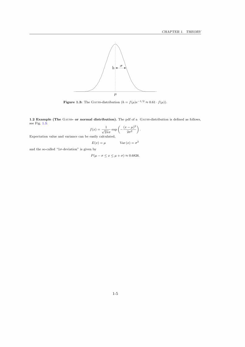
Figure 1.3: The Gauss-distribution (h = f(µ)e−1/2 ≈ 0.61 · f(µ)).
1.2 Example (The Gauss- or normal distribution). The pdf of a Gauss-distribution is defined as follows,see Fig. 1.3:
f(x) =1√2πσ
exp
„
− (x − µ)2
2σ2
«
.
Expectation value and variance can be easily calculated,
E(x) = µ Var (x) = σ2
and the so-called “1σ-deviation” is given by
P (µ − σ ≤ x ≤ µ + σ) ≈ 0.6826.
1-5

CHAPTER 1. THEORY
1.2 Some random remarks about random numbers
In this section, we will briefly discuss how to construct simple random number generators (RNGs)and how to test them. At first, let us consider the requirements for useful random numbers.Strictly speaking, there are three different classes of random numbers, namely
• real random numbers, e.g., obtained from radio-active decays (laborious, few)
• pseudo random numbers, calculated from a deterministic algorithm, and
• sub-random numbers, which have an “optimal” uniform distribution, but are not com-pletely independent (for an introduction, see Numerical Recipes). Sub-random numbersare particularly used for Monte Carlo integrations.
In the remainder of this section, we will concentrate on pseudo random numbers, which must/shouldsatisfy the following requirements:
• uniformly distributed
• statistically independent
• not or at least long-periodically (most algorithms produce random numbers with a certainperiod)
• reproducable (tests of programs!)
• portable: it should be possible to obtain identical results using different computers anddifferent programming languages.
• calculated by a fast algorithm.
The first three of these requirements are a “must”, whereas the latter ones are a “should”,which will be met by most of the RNGs discussed in this section, particularly by the “minimumstandard” RNG (see below).
1.2.1 (Multiplicative) linear congruential RNGs
For most “standard” tasks such as integrations and (astro-)physical simulations, the best choiceis to use so-called (multiplicative) linear congruential RNGs, because of their speed, though othermethods are availabe, mostly based on encryption methods, which, however, are much slower.
Basic algorithm.
SEED = (A · SEED + C) mod M (SEED, A, C, M integer-numbers) (1.16)
x = SEED/M normalization, conversion to real-number
• For any given initial value, SEED, a new SEED-value (“1st random number”) is calculated.From this value, a 2nd random number is created, and so on. Since SEED is always(integer mod M), we have
0 ≤ SEED < M, i.e., x ∈ [0, 1).
• The maximum value possible for this algorithm is M − 1.
1-6

CHAPTER 1. THEORY
• By construction, the algorithm implies a periodic behaviour: a new cycle starts, if
SEED(actual) = SEED(initial)
• Since this period should be as long as possible⇒M should roughly correspond to the maximum integer value which can be representedon the specific system.
• An optimum algorithm would produce all possible integers, 0 . . . M − 1, which, however,is not always the case.
At least for linear congruential RNGs with C > 0 it can be proven that the maximum possibleperiod, M , can be actually created if certain (simple) conditions relating C, A and M aresatisfied.
1.3 Example (Algorithms with C > 0 and M = 2n).
• n ≤ 31 for 4-byte integers (note: only positive/zero integers are used)
• As an example, A = 5 and C = 1 satisfy the required conditions if n ≥ 2 (other combinations are possibleas well). In the following we consider the cycle with n = 5, i.e., M = 32.
• According to the above statement, the maximum possible cycle (→ 32 different numbers) should be pro-duced by using these values, which is actually the case, as shown in Tab. 1.1
SEED (start) = 9
SEED (1) = 5 · 9 + 1 mod 32 = 46 mod 32 = 14, etc.,
↓ 9 1 25 17 9 (← new cycle)14 6 30 22 147 31 23 15 74 28 20 12 ·
21 13 5 29 ·10 2 26 18 ·19 11 3 270 24 16 8
Table 1.1: Random number sequence SEED = (5 · SEED + 1) mod 32 with initial value 9.
The problem of portability.
Since we are aiming at a rather long cycle, (M − 1) should correspond to the maximum integer
which can be represented on a specific machine (231 − 1 for 4-byte integers). Because of (1.16),the calculation of SEED requires the evaluation of intermediate results being larger than M − 1(“overflows”) so that the algorithm would fail (e.g, if SEED becomes of order M). In the abovecycle, this problem would already occur for the first number calculated, 46 mod 32.
A possible solution would comprise an assembly language implementation of our algorithm,with 8-byte product registers. In this case, however, the algorithm would be no longer portable(implementation is machine dependent).
A way out of this dilemma was shown by Schrage (1979). He devised a method by whichmultiplications of type
(A · SEED) mod M, (1.17)
1-7

CHAPTER 1. THEORY
with A, SEED and M consisting of a certain length (e.g., 4 byte), can be calculated withoutoverflow.
This “trick”, however, implies that our algorithm has to get along with C ≡ 0. As a firstconsequence, SEED = 0 is prohibited, and x ∈ (0, 1).
In dependence of M , again only certain values of A are “allowed” to maintain the requiredproperties of the RNG. For M = 2n, e.g., long cycles are possible (though being at least afactor of 4 shorter than above), but most of these cylces inhibit certain problems, particularlyconcerning the independence of the created numbers. An impressive example of such problemsis given in example 1.11.
Thus, for C = 0 we strongly advise to avoid M = 2n and to use alternative cycles with Mbeing a prime number. In this case then, a maximum period of M −1 (no “zero”) can be createdif A is chosen in a specific, rather complex way. The corresponding sequence has a long period,uniform distribution and almost no correlation problem, as discussed below.
1.2.2 The minimum-standard RNG
Based on these considerations, Parkand Miller (1988) suggested to use the following, mostsimple RNG for the case C ≡ 0, called “minimum-standard” generator. In particular,
M = 231 − 1 = 2147483647,
which, on the one hand, is the largest representable 4-byte integer, and, on the other, is alsoa prime number. This lucky situation is not a pure coincidence, since the above number is aso-called Mersenne prime number.1
With this value of M , one obtains roughly 2.15 · 109 different random numbers ∈ (0, 1), whenA is given by one of the following numbers,
A =
16807 = 75
48271
69621.
All three values comply to both the complex requirement for allowing the maximum period andone additional condition which arises if Schrage’s “trick” shall be applied.
Advanced reading: Schrage’s multiplication, (A · SEED) mod M
At first, M must be decomposed in the following way:
M = A · q + r with q =
[M
A
]
, (1.18)
where square brackets denotes an integer-operation. In this way then,
r = M mod A.
1.4 Example. Let M = 231 − 1 and A = 16807. Then
q =
»M
A
–
= 127773
r = M mod A = 2836
and thusM = 16807 · 127773 + 2836 = 231 − 1.
1If p is prime, then in many but not all cases 2p − 1 is also prime. In such a case, this number is called aMersenne prime number.
1-8

CHAPTER 1. THEORY
With these definitions of q and r, the following theorem can be proven:
1.5 Theorem. If r < q (this is the additional condition) and 0 < SEED < M− 1, then
(i)
A · (SEED mod q)
r ·[SEED
q
]
}
< M − 1, (1.19)
can be calculated without overflow! We are now looking for
SEEDnew = (A · SEED) mod M. Let
DIFF := A · (SEED mod q)− r ·[SEED
q
]
. (1.20)
Because of (1.19) it is also ensured that
|DIFF| < M− 1
can be calculated without overflow as well.
(ii) The random number SEEDnew finally results via
SEEDnew =
{
DIFF, if DIFF > 0
DIFF + M, if DIFF < 0.(1.21)
1.6 Example (simple). Calculation of (3 · 5) mod 10 without overflow corresponding to an intermediate value> (M − 1) = 9 (A = 3 and SEED = 5):
q =ˆ103
˜= 3
r = 10 mod 3 = 1
ff
thus r < q and SEED < M− 1 = 9.
The requirements are satisfied, and with (1.20, 1.21) we find
(A · SEED) mod M = A · (SEED mod q) − r
»SEED
q
–
= 3 · 2|{z}
<M−1
− 1 · 1|{z}
<M−1
= 5.
1.7 Example (typical). M = 231 − 1 = 2147483647, SEED = 1147483647, A = 69621. Direct calculation yields
SEEDnew = 79888958987787| {z }
>M(∗)
mod M = 419835740,
where (∗) cannot be represented with 4 bytes.
Using Schrage’s trick, we obtain, without overflow
DIFF = A(SEED mod M) − r
»SEED
q
–
= 1309014042| {z }
<M−1
−889178302
= 419835740!= SEEDnew.
1-9

CHAPTER 1. THEORY
Algorithm for the Park-Miller minimum-standard generator and Schrage’s multiplica-tion:
RAN(ISEED)
Real RAN
Integer (4 Byte), Parameter2:: M = 2147483647, A = 69621, q = 30845, r = 23902
Real, Parameter:: M1 = 1./Float(M)
Integer (4 Byte):: ISEED, K
K = ISEED / q
ISEED = A * (ISEED - K * q) - r * K
IF (ISEED < 0) ISEED = ISEED + M
RAN = ISEED * M1
END
Note that (ISEED - K * q) corresponds to the operation SEED mod q.
To calculate a random number with this generator, only four statements are required, the restare declarations! Before the first call of RAN, the variable ISEED has to be initalized, with 0 <ISEED < M − 1. From then on, ISEED must not be changed except by RAN itself!
1.2.3 Tests of RNGs
In order to check for the reliability of any unknown RNG, a number of tests should be per-formed. In particular, one has to confirm that the random numbers provided by the generatorare uniformly distributed and statistically independent from each other.
Two rather simple possibilities will be described in the following, namely the calculation ofPearson’s χ2
p (which asymptotically corresponds to the “usual” χ2, and a graphical test. Wewill see that all RNGs based on the linear congruential algorithm (1.16) suffer from a certaindeficiency, which can be cured in a simple and fast way by the so-called “reshuffling” method.
1.2.3.1 Advanced reading: Test of uniform distribution
At first, one has to check whether the created random numbers are uniformly distributed in(0, 1). Remember that a uniform distribution implies a constant pdf within this interval, i.e.,
p(x)dx = dx,
cf. Sect. 1.1.3. At first let us consider the following, more general problem. Let Ni, i = 1, . . ., kwith
k∑
i=1
Ni =: N
the number of outcomes regarding a certain event i during an “experiment”. We like to test theprobability that a particular value of Ni corresponds to a given number ni.
1.8 Example (Test of dices). Let’s roll the dice and define
N1 number of events with outcome 1, . . . , 4,
N2 number of events with outcome 5 and 6,
N = N1 + N2.
2corresponding to a globale constant in C++
1-10

CHAPTER 1. THEORY
We will test whether N1 and N2 are distributed according to the expectation, n1 = 23N , n2 = 1
3N , i.e., whether
the dice has not been manipulated.
Method. To perform such a test, Pearson’s χ2p has to be calculated
χ2p =
k∑
i=1
(Ni − ni)2
ni. (1.22)
For this quantity, the following theorem can be proven (actually, this proof is rather complex).
1.9 Theorem. Pearson’s χ2p (1.22) is a statistical function, which asymptotically (i.e., for
Ni À 1 ∀ i) corresponds to the sum of squares of f independent random variables, which arenormally distributed, with expectation value 0 and variance 1. The degrees of freedom, f , aredefined by
• if ni is fixed, we have f = k.
• if ni is normalized via∑
ni =∑
Ni = N , we have f = k − 1 ( one constraint).
• if m additional constraints are present, we have f = k −m− 1.
Because of this theorem, Pearson’s χ2p asymptotically corresponds to the “usual” χ2-distribution,
well-known from optimization/regression methods. Remember that the expectation value of χ2
is f and that the standard deviation of χ2 is√
(2f). In praxis, “asymptotically” means that ineach “channel” i at least ni = 5 events are to be expected.
1.10 Example (Continuation: Test of dices). With Ni, ni, i = 1, 2 as given above, Pearson’s χ2p results in
χ2p =
X (Ni − ni)2
ni=
(N1 − 23N)2
23N
+(N2 − 1
3N)2
13N
.
Because of the requirement that one has to expect at least five events in each channel, we have to throw the diceat least N = 15 times. Thus, we have
χ2p =
(N1 − 10)2
10+
(N2 − 5)2
5,
and the degrees of freedom are f = 2 − 1 = 1.
Let’s test now four different dices. After 15 throws each we obtained the results given in Tab. 1.2. The quantity Qgives the probability that by chance a larger value of χ2 (larger than actually found) could have been present. IfQ has a reasonable value (typically, within 0.05. . . 0.95), everything should be OK, whereas a low value indicatesthat the actual χ2 is too large for the given degrees of freedom (dice faked!). Concerning the calculation of Q,see Numerical Recipes, chap. 6.2. Note that for an unmanipulated dice, < χ2 >≈ 1 ±
√2 is to be expected.
dice N1 N2 χ2p Q(χ2
p, f = 1)
1 10 5 0 12 1 14 24.3 8.24 ·10−7
3 4 11 10.8 10−3
4 8 7 1.2 0.27
Table 1.2: Test of four different dices
The results of our “experiment” can be interpreted as follows:
d1ce 1: The outcome is “too good”, throw the dice once more. Too good (χ2 = 0)) means that the result is“exactly” as one expects. Usually, such a result is only obtained if the experiment has been faked.
d2ce 2: The outcome is very unprobable, and the dice can be suspected to be manipulated.
d3ce 3: The outcome is unprobable, however still possible. Throw the dice once more.
d4ce 4: The result is OK, and the dice seems to be ummanipulated.
1-11

CHAPTER 1. THEORY
Comment. To obtain a larger significance regarding our findings, the experiment should beperformed a couple of times (say, at least 10 times). The specific results have then to be checkedversus the expectation that the individual χ2 must follow the χ2-distribution for f degrees offreedom, if the dices were unmanipulated (see below).
An alternative formulation of Pearson’s χ2p is given by
χ2p =
k∑
i=1
(Ni − ni)2
ni=
k∑
i=1
(Ni − piN)2
piN, (1.23)
where
• k is the number of “channels” (possible events)
• Ni the number of events in channel i with∑
i
Ni = N ,
• pi the probability for the event in channel i.
The channels must be selected in such a way that all possible events can be accounted for, i.e.,
that∑
i
pi = 1.
Application to random numbers. Remember the original question whether the providedrandom numbers are uniformly distributed within (0, 1). To answer this question, we “bin” the
interval (0, 1) into k equally wide sub-intervals. We calculate N random numbers and distributethem according to their values into the corresponding channels. After the required number ofrandom numbers has been drawn (see below), we count the occurence Ni in each channel. If the
random numbers were uniformly distributed, we should have pi =1
kfor all i.
Thus, we calculate
χ2p =
k∑
i=1
(Ni − Nk )2
N/k,
such that in each channel the expected value of ni = N/k is at least 5, i.e, a minimum of N = 5krandom numbers have to be drawn. Then,
• the probability Q(χ2p, k − 1) has to be calculated, and
• the test has to be repeated l times, with typically l ≈ 10. Note, that the initial SEED valuehas to be different for different l, of course.
• At last, we test whether the individual χ2p,j(j = 1, . . . , l) within the series are distributed
according to χ2 with k − 1 degrees of freedom. This can be obtained by the so-calledKolmogoroff-Smirnov-test. 3
• If the indivual Qj values are “reasonable” and the Kolmogorroff-Smirnov-test hasyielded a “reasonable” probability as well, the RNG provides indeed uniformly distributedrandom numbers, at least with respect to the defined channels.
3e.g., Numerical Recipes, chap. 14.3
1-12
CHAPTER 1. THEORY
�����������
�����������
�����������
���
���
PSfrag replacements
0
1
1
x1, x2
x3, x4
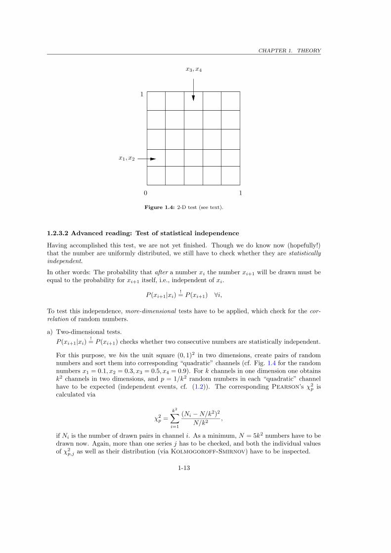
Figure 1.4: 2-D test (see text).
1.2.3.2 Advanced reading: Test of statistical independence
Having accomplished this test, we are not yet finished. Though we do know now (hopefully!)that the number are uniformly distributed, we still have to check whether they are statisticallyindependent.
In other words: The probability that after a number xi the number xi+1 will be drawn must beequal to the probability for xi+1 itself, i.e., independent of xi.
P (xi+1|xi)!= P (xi+1) ∀i,
To test this independence, more-dimensional tests have to be applied, which check for the cor-relation of random numbers.
a) Two-dimensional tests.
P (xi+1|xi)!= P (xi+1) checks whether two consecutive numbers are statistically independent.
For this purpose, we bin the unit square (0, 1)2 in two dimensions, create pairs of randomnumbers and sort them into corresponding “quadratic” channels (cf. Fig. 1.4 for the randomnumbers x1 = 0.1, x2 = 0.3, x3 = 0.5, x4 = 0.9). For k channels in one dimension one obtainsk2 channels in two dimensions, and p = 1/k2 random numbers in each “quadratic” channelhave to be expected (independent events, cf. (1.2)). The corresponding Pearson’s χ2
p iscalculated via
χ2p =
k2
∑
i=1
(Ni −N/k2)2
N/k2,
if Ni is the number of drawn pairs in channel i. As a minimum, N = 5k2 numbers have to bedrawn now. Again, more than one series j has to be checked, and both the individual valuesof χ2
p,j as well as their distribution (via Kolmogoroff-Smirnov) have to be inspected.
1-13

CHAPTER 1. THEORY
b) Three-dimensional tests.
P (xi+2|xi+1, xi)!= P (xi+2) checks for the independence of a third random number from
the previously drawn first and second one. In analogy to a) and b), we consider the unitcube (0, 1)3. Triples of three consecutive random numbers are sorted into this cube, and thecorresponding probability is given by pi = 1/k3. The further proceeding is as above.
c) Typically, up to 8 dimensions should be checked for a rigorous test of a given RNG. (Whatproblem might arise?) Check the web for published results.
1.11 Example (RANDU: A famous failure). One of the first RNGs which have been implemented on a computer,RANDU (by IBM!), used the algoritm (1.17) with M = 231, A = 65539 and C = 0, i.e., an algorithm which hasbeen discussed as being potentially “dangerous” (remember that the minimum-standard generator uses a primenumber for M). Though the above tests for 1- and 2-D are passed without any problem, the situation is differentfrom the 3-D case on (it seems that IBM did not consider it as necessary to perform this test).
In the following, we carry out such a 3-D test with 303 = 27 000 channels and 270 000 random numbers. Thus,N/(303) = 10 events per channel are to be expected, and a value of χ2 of the order of f = (27 000 − 1) shouldresult for an appropriate RNG. We have calculated 10 test series each for the Park/Miller minimum-standardgenerator and for RANDU. Below we compare the outcome of our test.
Park/Miller Minimum-Standard
----------------------------
chi2 = 26851.98 Q = 0.7373354
chi2 = 27006.20 Q = 0.4844202
chi2 = 26865.37 Q = 0.7192582
chi2 = 27167.66 Q = 0.2369688
chi2 = 26666.29 Q = 0.9249226
chi2 = 27187.38 Q = 0.2070863
chi2 = 27079.77 Q = 0.3661267
chi2 = 26667.37 Q = 0.9247663
chi2 = 27142.82 Q = 0.2668213
chi2 = 27135.24 Q = 0.2786968
The probability that the values for χ2p do follow the χ2-distribution is given (via Kolmogoroff-Smirnov) by
KS-TEST: prob = 0.7328884.
Thus, as it is also evident from the individual values of χ2p alone, being actually of the order of ≈ 27, 000, we
conclude that the minimum-standard generator passes the 3-D test. In contrast, RANDU. The corresponding resultsare given by
RANDU
-----
chi2 = 452505.8 Q = 0.0000000E+00 (in single precision)
chi2 = 454412.7 Q = 0.0000000E+00
chi2 = 456254.8 Q = 0.0000000E+00
chi2 = 454074.1 Q = 0.0000000E+00
chi2 = 452412.2 Q = 0.0000000E+00
chi2 = 452882.0 Q = 0.0000000E+00
chi2 = 453038.7 Q = 0.0000000E+00
chi2 = 455033.4 Q = 0.0000000E+00
chi2 = 453992.2 Q = 0.0000000E+00
chi2 = 453478.2 Q = 0.0000000E+00
(note that each individual value of χ2p correspond to ≈ 17 · f) and the KS-test yields
KS-TEST: prob = 5.546628E-10 (!!!)
1-14

CHAPTER 1. THEORY
Figure 1.5: 2-D representation of random numbers, created via SEED = (65 ∗ SEED+ 1) mod 2048. The numbersare located on 31 hyper-surfaces.
i.e., the probability is VERY low that the individual χ2p follow a χ2 distribution with f ≈ 27, 000. Though RANDU
delivers numbers which are uniformely distributed (not shown here), each third number is strongly correlatedwith the two previous ones. Consequently, these numbers are not statistically independent and therfore no
pseude-random numbers!
1.2.3.3 Graphical representation
One additional/alternative test is given by the graphical representation of the drawn randomnumbers. From such tests, a deficiency becomes obvious which affects all random numberscraeated by linar congruential algorithms: If one plots k consecutive random numbers in a k-dimensional space, they do not fill this space uniformely, but are located on (k− 1)-dimensionalhyper-surfaces. It can be shown that the maximum number of these hyper-surfaces is given byM1/k, where only a careful choice of A and C ensures that this maximum is actually realized.
In Fig. 1.5 we display this deficiency by means of a (short-period) generator with algorithm
SEED = (65 ∗ SEED + 1) mod 2048.
With respect to a 2-D representation, the maximum number of hyper-surfaces (here: straightlines) is given by 20481/2 ≈ 45. With our choice of A = 65 and C = 1, at least 31 of thosehyper-surfaces are realized.
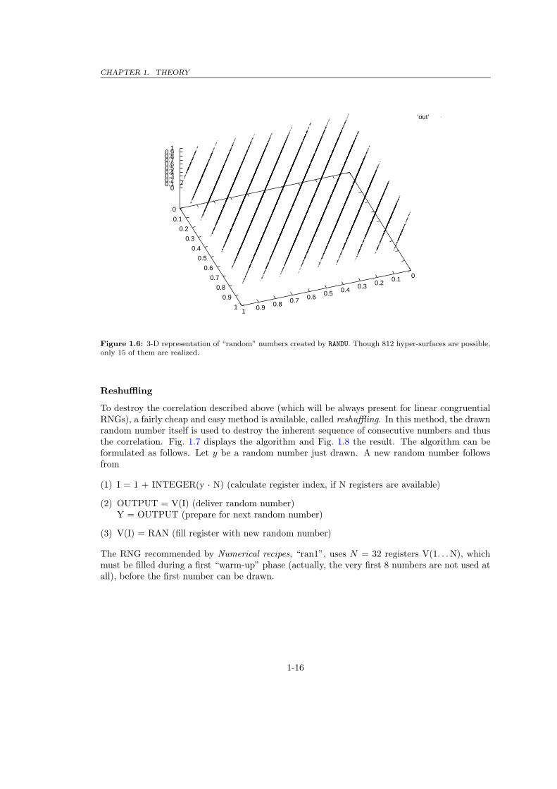
If M = 231, a 3-D representation should yield a maximum number of (231)1/3 ≈ 1290 surfaces.For RANDU (see example 1.11), this number becomes reduced by a factor of 41/3, because onlyeven numbers and additionally only half of them can be created, thus reducing the maximumnumber of surfaces to 812. In contrast however, this generator delivers only 15! surfaces (seeFig. 1.6), i.e., the available space is by no means uniformly filled, which again shows the failureof RANDU.
1-15
CHAPTER 1. THEORY
’out’
00.10.20.30.40.50.60.70.80.91
0
0.1
0.2
0.3
0.4
0.5
0.6
0.7
0.8
0.9
1
00.10.20.30.40.50.60.70.80.9
1
Figure 1.6: 3-D representation of “random” numbers created by RANDU. Though 812 hyper-surfaces are possible,only 15 of them are realized.
Reshuffling
To destroy the correlation described above (which will be always present for linear congruentialRNGs), a fairly cheap and easy method is available, called reshuffling. In this method, the drawnrandom number itself is used to destroy the inherent sequence of consecutive numbers and thusthe correlation. Fig. 1.7 displays the algorithm and Fig. 1.8 the result. The algorithm can beformulated as follows. Let y be a random number just drawn. A new random number followsfrom
(1) I = 1 + INTEGER(y · N) (calculate register index, if N registers are available)
(2) OUTPUT = V(I) (deliver random number)Y = OUTPUT (prepare for next random number)
(3) V(I) = RAN (fill register with new random number)
The RNG recommended by Numerical recipes, “ran1”, uses N = 32 registers V(1. . . N), whichmust be filled during a first “warm-up” phase (actually, the very first 8 numbers are not used atall), before the first number can be drawn.
1-16

CHAPTER 1. THEORY
PSfrag replacements
(1)
(2)(3)
RAN OUTPUT
V(1)
V(I)
V(N)
y
N registers (first filling during “warm up”)
Figure 1.7: Reshuffling algorithm
Figure 1.8: As Fig. 1.5, but with reshuffling. Any previous correlation has been destroyed.
1-17

CHAPTER 1. THEORY
1.3 Monte Carlo integration
After having discussed the generation of random numbers, we will discuss the Monte Carlointegration in this section, as a first and important application of Monte Carlo methods. Suchan integration can replace more common methods based on well-known integration formulae(Trapez, Simpson etc.) and should be used under certain conditions, as outlined in Sect. 1.3.3.
1.3.1 Preparation
Before we can start with the “real” stuff, we need some preparatory work in order to understandthe basic ideas. Impatient readers might immediately switch to Sect. 1.3.2.
• Let us begin by drawing N variates (= random variables) x1, . . . , xN from a given pdf f(x),e.g., from the uniform distribution of pseudo random numbers as created by a RNG. Forarbitrary pdfs, we will present the corresponding procedure in Sect. 1.4.
• From these variates, we calculate a new random variable (remember that functions ofrandom variables are random variables themselves) by means of
G =N∑
n=1
1
Ng(xn), (1.24)
where g is an arbitrary function of x. Since the expectation value is a linear operator, theexpectation value of G is given by
E(G) = G =
N∑
n=1
1
NE(g(xn)) = g, (1.25)
i.e, is the expectation value of g itself. The variance of G, on the other hand, is given by
Var (G) = Var
(N∑
n=1
1
Ng(xn)
)
=
N∑
n=1
1
N2Var (g(xn)) =
1
NVar (g) , (1.26)
where we have assumed that the variates are statistically independent (cf. 1.7). Note thatthe variance of G is a factor of N lower than the variance of g.
• Besides being a random variable, G (1.24) is also the arithmetical mean with respect to thedrawn random variables, g(xn). In so far, (1.25) states that the expectation value of thearithmetic mean of N random variables g(x) is nothing else than the expectation value ofg itself, independent of N .
• This will be the basis of the Monte Carlo integration, which can be defined as follows:
Approximate the expectation value of a function by the arithmetic mean over the corre-sponding sample!!!
g = G ≈ G
• Eq. 1.26 can be interpreted similarly: The variance of the arithmetical mean of N (inde-pendent!) random variables g(x) is lower than the variance of g(x) itself, by a factor of1/N . Note that statistically independent variates are essential for this statement, whichjustifies our effort concerning the corresponding tests of RNGs (Sect. 1.3.2.2).
1-18

CHAPTER 1. THEORY
Implication: The larger the sample, the smaller the variance of the arithmetical mean, andthe better the approximation
g ≈ G.
Note in particular that
G ≈ G±√
Var (G), i.e., G→ G = g for N →∞.
(Remember that Var (G) is the mean square deviation of G from G)
Summary. Before applying this knowledge within the Monte Carlo integration, we like tosummarize the derived relations.
pdf f(x)random variable g(x)
}E(g)
Var (g)
{true expectation valuetrue variance
E(g) = g =
∫
g(x)f(x)dx
Var (g) =
∫
(g(x)− g)2f(x)dx
Draw N variates, xn, n = 1, . . . , N according to f(x) and calculate the arithmetical mean,
G =1
N
N∑
n=1
g(xn).
Then we have
G = E(G) = E(g) = g
Var (G) =1
NVar (g)
σ(G) = (Var (G))1/2
=1√N
σ(g)
The last identity is known as the “1/√
N -law” of the Monte Carlo simulation. The actual “trick”now is the
Monte Carlo approximation: Approximate g = G by G
1.3.2 The method
The reader might question now in how far these statements concerning expectation values andvariances have to do with real integration problems. This will become clear in a second, by a(clever) re-formulation of the integral I to be evaluated:
I =
b∫
a
g(x)dx =
b∫
a
g(x)
f(x)f(x)dx =
b∫
a
h(x)f(x)dx (1.27)
1-19

CHAPTER 1. THEORY
The actual trick is now to demand that f(x) shall be a probability density function (pdf). Inthis way then, any integral can be re-interpreted as the expectation value of h(x) with respectto f(x), and we just have learnt how to approximate expectation values!
Until further notification, we will use a constant pdf, i.e., consider a uniform distribution overthe interval [a, b],
f(x) =
1
b− aa ≤ x ≤ b
0 else,
cf. (1.12). The “new” fuction h(x) is thus given by
h(x) =g(x)
f(x)= (b− a)g(x),
and the integral becomes proportional to the expectation value of g:
I = (b− a)
b∫
a
g(x)f(x)dxexact!= (b− a)g. (1.28)
We like to stress that this relation is still exact. In a second step then, we draw N variatesxn, n = 1, . . . , N according to the pdf (which is almost nothing else than drawing N randomnumbers, see below), calculate g(xn) and evaluate the corresponding arithmetical mean,
G =1
N
N∑
n=1
g(xn).
Finally, the integral I can be easily estimated by means of the Monte Carlo approximation,
I = (b− a)gexact= (b− a)G
Monte Carlo
approx.≈ (b− a)G. (1.29)
Thus, the established Monte Carlo integration is the (arithmetical) mean with respect to N“observations” of the integrand, when the variates xn are uniformly drawn from the interval[a, b], multiplied by the width of the interval.
The error introduced by the Monte Carlo approximation can be easily estimated as well.
Var (G) =1
NVar (g) =
1
N
(
g2
‖
J
− g2
‖
G2
)
≈ 1
N(J −G2), (1.30)
if
J =1
N
N∑
n=1
g2(xn)
is the Monte Carlo estimator for E(J) = J = g2 and if we approximate g2 = G2
by G2.
If we identify now the error of the estimated integral, δI, with the standard deviation resultingfrom Var (G)4 (which can be proven from the “central limit theorem” of statistics), it is obviousthat this error follows the “1/
√N -law”, i.e.,
δI ∝ 1/√
N.
4multiplied by (b − a)
1-20

CHAPTER 1. THEORY
By generalizing the integration element dx to an arbitrary-dimensional volume element dV , wefind the following cooking recipe for the Monte Carlo Integration:
∫
V
gdV ≈ V
(
〈g〉 ±√
1
N
(
〈g2〉 − 〈g〉2))
(1.31)
if
〈g〉 = G =1
N
∑
n
g(xn)
⟨g2⟩
= J =1
N
∑
n
g2(xn)
and V is the volume of the integration region considered.
1.12 Example. [Monte Carlo integration of the exponential function] As a simple example, we will estimate theintegral
2Z
0
e−xdx = 1 − e−2 = 0.86467
via Monte Carlow integration.
(1) At first, we draw N random numbers uniformly distributed ∈ [0, 2] and “integrate” for the two cases, a)N = 5 and b) N = 25. Since the RNG delivers numbers distributed ∈ (0, 1), we have to multiply them by afactor of 2, cf. Sect. 1.4, Eq. 1.41. Assume that the following variates have been provided.
Case a) Case b)
1 7.8263693E-05 1 0.1895919
2 1.3153778 2 0.4704462
3 1.5560532 3 0.7886472
4 0.5865013 4 0.7929640
5 1.3276724 5 1.3469290
6 1.8350208
7 1.1941637
8 0.3096535
9 0.3457211
10 0.5346164
11 1.2970020
12 0.7114938
13 7.6981865E-02
14 1.8341565
15 0.6684224
16 0.1748597
17 0.8677271
18 1.8897665
19 1.3043649
20 0.4616689
21 1.2692878
22 0.9196489
23 0.5391896
24 0.1599936
25 1.0119059
(2) We calculate
G = 〈g〉 =1
N
X
e−Xn
J =˙g2¸
=1
N
X“
e−Xn
”2,
1-21

CHAPTER 1. THEORY
with the following resultsa) G = 0.4601251, J = 0.2992171b) G = 0.4904828, J = 0.2930297
(3) With
I ≈ V
〈g〉 ±r
1
N
“
〈g2〉 − 〈g〉2”!
and “volume” V = 2, the integral is approximated by
Case a) I ≈ 0.9202501 ± 0.2645783Case b) I ≈ 0.9809657 ± 0.091613322.
Note that the “1/√
N-law” predicts an error reduction by 1/√
5 = 0.447, not completely met by our simulation,since case a) was estimated based on a very small sample. Morever, the result given for case b) represents “reality”only within a 2-sigma error.
The error for N = 25 is of the order of ±0.1. Thus, to reduce the error to ±0.001 (factor 100), the sample sizehas to be increased by a factor of 1002, i.e., we have to draw 250 000 random numbers.
The result of such a simulation (note that the RNG has to be fast) for N = 250 000 is given byG = 〈g〉 = 0.4322112, J =
˙g2¸
= 0.2453225, thus
I = 0.8644224 ± 0.9676 · 10−3.
We see that the (estimated) error has decreased as predicted, and a comparison of exact (I(exact) = 0.86476)and Monte Carlo result shows that it is also of the correct order.
As a preliminary conclusion then, we might state that the MC integration can be quickly pro-grammed but that a large number of evalutions of the integrand are necessary to obtain areasonable accuracy.
1.3.3 When shall we use the Monte Carlo integration?
Because of this large number of evaluations (and the corresponding computational time, even ifthe RNG itself is fast), one might question whether and when the Monte Carlo integration willbe advantageous to standard quadrature methods such as exploiting the Simpson- or Trapez-rule. At first let us remind that the “1/
√N -law” of the MC integration error is independent
of the dimensionality of the problem, in contrast to errors resulting from standard quadraturemethods.5 In the latter case (and assuming simple boundaries, simple integration formulae andequidistant step-sizes), the integration errors scales via
δI ∝ N−2d Trapez
δI ∝ N−4d Simpson, (1.32)
for N equidistant sampling points and dimensionality d.
Thus, the error of the standard quadrature (with equidistant step size) increases from ∼ N−2(4)
for 1-D over ∼ N−1(2) for 2-D to ∼ N−23( 43) for 3-D integrals, whereas the MC integration always
scales with ∼ N−1/2. Only from d = 5 (Trapez) or d = 9 (Simpson) on, the MC error decreasesfaster than the standard quadrature error. Before concluding that the MC integration is useless,however, one should consider the following arguments:
5though a rigorous error analyis for more-D integration is very complex, e.g., Stroud, A.H., 1971, Approximate
Calculation of Multiple Integrals, Prentice-Hall.
1-22

CHAPTER 1. THEORY
PSfrag replacements
area A with N points
∫
f(x)dx
Figure 1.9: “Hit or miss”-method for the evaluation of 1-D integrals.
• Just for more-D integrals complex boundaries are the rule (difficult to program), and theMC integration should be preferred, as long as the integrand is not locally concentrated.
• If the required precision is low, and particularly for first estimates of unknown integrals,the MC integration should be preferred as well, because of its simplicity.
• If the specific integral must be calculated only once, again the MC solution might beadvantegous, since the longer computational time is compensated by the greatly reducedprogramming effort.
1.3.4 Complex boundaries: “hit or miss”
To evaluate more-D integrals with complex boundaries, an alternative version of the MC inte-gration is usually employed, knows as “hit or miss”-method. At least the principal procedureshall be highlighted here, for the 1-D case and by means of Fig. 1.9. To evaluate the integralI =
∫f(x)dx,
• N points with co-ordinates (xi, yi) are uniformely distributed across the rectangle witharea A, by means of random numbers.
• All those points are counted as “hits” that have a y-co-ordinate with
yi ≤ f(xi) (1.33a)
If n hits have been counted in total, the integral can be easily approximated from
I =
∫
f(x)dx ≈ A · n
N. (1.33b)
1-23

CHAPTER 1. THEORY
• A disadvantage of this method is of course that all (N − n) points being no “hit” (i.e.,which are located above f(x)) are somewhat wasted (note that f(x) has to be evaluatedfor each point). For this reason, the circumscribing area A has to be chosen as small aspossible.
• The generalization of this method is fairly obvious, for typical examples see “Numericalrecipes”. E.g., to calculate the area of a circle, one proceeds as above, however now countingthose points as hits on a square A which satisfy the relation x2
i + y2i ≤ r2, for given radius
r. Again, the area of the circle results from the fraction A nN .
1.3.5 Advanced reading: Variance reduction – Importance sampling
The large number of required sampling points, being the consequence of a rather slow decreasein error (∝ N−1/2) and giving rise to relatively large computational times, can be somewhatdecreased by different methods. The most important ones make use of the so-called stratifiedsampling and importance sampling, respectively (mixed strategies are possible as well). Theformer approach relies on dividing the integration volume into sub-volumes, calculating the MCestimates for each individual sub-volume and adding up the results finally. If the sub-volumesare chosen in a proper way, the individual variances can add up to a total variance which issmaller than the variance obtained for an integration of the total volume. More information canbe obtained from Numerical Recipes, Chap. 7.8.
In the following, we will have a closer look into the importance sampling approach. Rememberthat the integration error does not only contain the scaling factor N−1/2, but depends also onthe difference
(< g2 > − < g >2),
if g is the function to be integrated and angle brackets denote arithmetic means. It is this factorwhich can be reduced by importance sampling, sometimes considerably.
The basic idea is very simple. Remember that the integral I had been re-interpreted as anexpectation value regarding a specified pdf p,
I =
∫
gdV =
∫g
ppdV.
Instead of using a uniform distribution, i.e., a constant pdf, we will now use a different pdf p,chosen in such a way as to decrease the variance. Since any pdf has to be normalized, one alwayshas to consider the constraint ∫
pdV = 1. (1.34)
For arbitrary pdf’s p then, the generalization of (1.31) is straightforward, and the Monte Carloestimator of the integral is given by
I = 〈gp〉 ± 1√
N
(
〈(g
p)2〉 − 〈g
p〉2) 1
2
, (1.35)
where < g/p > is the arithmetic mean of g(xn)/p(xn), and the variates xn have been drawnaccording to the pdf p! Note in particular that any volume factor has vanished. From thisequation, the (original) variance can be diminished signficantly if the pdf p is chosen in such away that it is very close to g, i.e., if
g
p≈ constant over the integration region.
1-24

CHAPTER 1. THEORY
If p = g, the variance would become zero, and one might think that this solves the problemimmediately. As we will see in the next section, however, the calculation of variates according toa pdf p requires the calculation of
∫pdV , which, for p = g, is just the integral we actually like
to solve, and we would have gained nothing.
Instead of using p = g then, the best compromise is to use a pdf p which is fairly similar to g,but also allows for a quick an easy calculation of the corresponding variates.
Finally, we will show that our MC cooking recipe (1.31) is just a special case for the abovegeneralization, Eq. 1.35, under the restriction that p is constant. Because of the normalization(1.34), we immediately find in this case that
p =1
V,
and
I =
∫
gdV ≈ 〈 g
1/V〉 ± 1√
N
(
〈( g
1/V)2〉 − 〈 g
1/V〉2) 1
2
= V
(
< g > ± 1√N
(< g2 > − < g >2)12
)
, q.e.d.
1-25

CHAPTER 1. THEORY
1.4 Monte Carlo simulations
We are now (almost) prepared to perform Monte Carlo simulations (in the literal sense of theword). At first, let us outline the basic “philosophy” of such simulations.
1.4.1 Basic philosophy and a first example
• Assume that we have a compley physical (or economical etc.) problem, which cannot (oronly with enormous effort) be solved in a closed way.
• Instead, however, we do know the “physics” of the constituating sub-processes.
• These individual sub-processes are described by using pdf’s, and combined in a proper wayas to describe the complete problem. The final result is then obtained from multiple runsthrough the various possible process-chains, in dependence of the provided pdf’s (whichare calculated from random numbers).
• After having followed a sufficient number of runs, we assume that the multitude of outcomeshas provided a fair mapping of “reality”, and the result (plus noise) is obtained fromcollecting the output of the individual runs.
advantages: Usually, such a method can be programmed in a fast and easy way, and results ofcomplicated problems can be obtained on relatively short time-scales.
disadvantages: On the other hand, a deeper understanding of the results becomes rather diffi-cult, and no analytical approximation can be developed throughout the process of solution.In particular, one has to perform a completely new simulation if only one of the parame-ters might change. Moreover, the reliability of the results depends crucially on a “perfect”knowledge of the sub-processes and a proper implementation of all possible paths whichcan be realized during the simulation.
1.13 Example (Radiative transfer in stellar atmospheres). Even in a simple geometry, the solution of theequation of radiative transfer (RT) is non-trivial, and in more complex situations (more-D, no symmetry, non-homogenous, clumpy medium) mostly impossible. Because of this reason, Monte Carlo simulations are employedto obtain corresponding results, particularly since the physics of the subprocesses (i.e., the interaction betweenphotons and matter) is well understood.
As an example we consider the following (seemingly trivial) problem, which - in a different perspective - will bereconsidered in the practical work to be performed.
We like to calculate the spatial radiation energy density distribution E(τ), in a (plane-parallel) atmosphericlayer, if photons are scattered by free electrons only. This problem is met, to a good approximation, in the outerregions of (very) hot stars.
One can show that this problem can be described by Milne’s integral equation,
E(τ) =1
2
∞Z
0
E(t)E1 |t − τ | dt, (1.36)
where E1(x) is the so-called first exponential integral,
E1(x) =
∞Z
1
e−x·t
tdt,
and τ the “optical depth”, here with respect to the radial direction (i.e., perpendicular to the atmosphere).
The optical depth is the relevant depth scale for problems involving photon transfer, and depends on theparticular cross-section(s) of the involved interactions(s), σ, and on the absorber densities, n. Since, for a given
1-26

CHAPTER 1. THEORY
PSfrag replacements
inside
outside
τ1
τ2
τ3
θ
Figure 1.10: Monte Carlo Simulation: radiative transfer (electron scattering only) in stellar atmospheres.
frequency, usually different interactions are possible, all these possibilites have to be accounted for in the calcula-tion of the optical depth. In the considered case (pure thomson-scattering), however, the optical depth is easilycalculated and moreover almost frequency independent, if we consider only frequencies being lower than X-rayenergies.
τ(s1, s2) =
r1Z
r2
σ n(s)ds, (1.37)
where the absorber density corresponds to the (free) electron density and the optical depth is defined between tospatial points with “co-ordinates” s1 and s2 and s is the geometrical length of the photon’s path.
Analytic and MC solution of Milne’s integral equation
Milne’s equation (1.36) can be exactly solved, but only in a very complex way, and the spatial radiative energydensity distribution (normalized to its value at the outer boundary, τ = 0) is given by
E(τ)
E(0)=
√3 (τ + q(τ)) . (1.38)
q(τ) is the so-called “Hopf-function”, with 1√3≤ q(τ) < 0.710446, which constitutes the real complicate part of
the problem.6
An adequate solution by a Monte Carlo simulation, on the other hand, can be realized as follows (cf. Fig. 1.10,for more details see Sect. 2.3):
• Photons have to be “created” emerging from the deepest layers, defined by τmax.
• The probability for a certain emission angle, θ (with respect to the radial direction), is given by
p(µ)dµ ∼ µdµ, µ = cos θ.
• The optical depth passed until the next scattering event can be described by the probability
p(τ)dτ ∼ e−τdτ,
(this is a general result for absorption of light) and
• the scattering angle (at low energies) can be approximated to be isotropic,
p(µ)dµ ∼ dµ.
6 Note that an approximate solution of Milne’s equation can be obtained in a much simpler way, wherethe only difference compared to the exact solution regards the fact that q(τ) results in 2/3, independentof τ (see., e.g., Mihalas, D., 1978, Stellar atmospheres, Freeman, San Francisco, or http://www.usm.uni-muenchen.de/people/puls/stellar at/stellar at.html, Chap. 3 and 4).
1-27
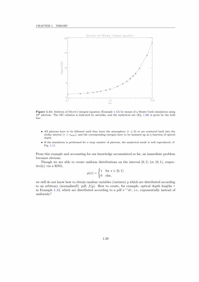
CHAPTER 1. THEORY
Figure 1.11: Solution of Milne’s integral equation (Example 1.13) by means of a Monte Carlo simulation using106 photons. The MC solution is indicated by asterisks, and the analytical one (Eq. 1.38) is given by the boldline.
• All photons have to be followed until they leave the atmosphere (τ ≤ 0) or are scattered back into thestellar interior (τ > τmax), and the corresponding energies have to be summed up as a function of opticaldepth.
• If the simulation is performed for a large number of photons, the analytical result is well reproduced, cf.Fig. 1.11.
From this example and accounting for our knowledge accumulated so far, an immediate problembecomes obvious:
Though we are able to create uniform distributions on the interval [0, 1) (or (0, 1), respec-tively) via a RNG,
p(x) =
{
1 for x ∈ [0, 1)
0 else,
we still do not know how to obtain random variables (variates) y which are distributed accordingto an arbitrary (normalized!) pdf, f(y). How to create, for example, optical depth lengths τin Example 1.13, which are distributed according to a pdf e−τdτ , i.e., exponentially instead ofuniformly?
1-28

CHAPTER 1. THEORY
PSfrag replacements
x
y
dx
dy
y(x)
Figure 1.12: The transformation method, see text. f(y)dy is the probability that y is in dy, and p(x)dx is theprobability that x is in dx.
1.4.2 Variates with arbitrary distribution
Actually, we encountered a similar problem already in example 1.12, where we were forced toconsider a uniform distribution on the interval [0,2] (instead of [0,1]), and in Sect. 1.3.5, where werequired the variates to be drawn from a specially designed pdf in order to reduce the variance.
Indeed, this problem is central to Monte Carlo simulations, and will be covered in the nextsection.
1.4.2.1 The inversion- or transformation method
Let p(x) and f(y) be different probability density functions (pdf’s)
p(x)dx = P (x ≤ x′ ≤ x + dx)
f(y)dy = P (y ≤ y′ ≤ y + dy)
with y = y(x): The random variable y shall be a function of the random variable x. A physicaltransformation means that corresponding probabilities, P , must be equal:
If p(x)dx is the probability that x is within the range x, x + dx and y is a function of x, thenthe probability that y is in the range y, y + dy must be the same!
1.14 Example. x shall be distributed uniformely in [0, 1], and y = 2x. The probability that x is in 0.1 . . . 0.2must be equal to the probability that y is in 0.2 . . . 0.4 (cf. Example 1.12).
Similarly, the probability that x ∈ [0, 1] (= 1) must correspond to the probability that y ∈ [0, 2] (also = 1).
From this argumentation, we thus have
|p(x)dx| = |f(y)dy| (1.39a)
or alternatively
f(y) = p(x)
∣∣∣∣
dx
dy
∣∣∣∣.
1-29

CHAPTER 1. THEORY
We have to use the absolute value because y(x) can be a (monotonically) increasing or de-creasing function, whereas probabilities have to be larger than zero by definition. The more-Dgeneralization of this relation involves the Jacobian of the transformation,
|p(x1, x2)dx1dx2| = |f(y1, y2)dy1dy2| ,
i.e.,
f(y1, y2) = p(x1, x2)
∣∣∣∣
∂(x1, x2)
∂(y1, y2)
∣∣∣∣
(1.39b)
Let now p(x) be uniformly distributed on [0, 1], e.g., x has been calculated by a RNG⇒ p(x) = 1.Then
dx = |f(y)dy| →x∫
0
dx′ =
∣∣∣∣∣∣∣
y(x)∫
ymin
f(y)dy
∣∣∣∣∣∣∣
⇒ x = F (y) =
∣∣∣∣∣
y∫
ymin
f(y′)dy′
︸ ︷︷ ︸cumulative prob.
distribution
∣∣∣∣∣
with F (ymin) = 0, F (ymax = y(1)) = 1.
Thus we find thaty = F−1(x), if x is uniformly distributed. (1.40)
In summary, the inversion-(or transformation-) method requires that F (y)
• can be calculated analytically and
• can be inverted.
To create a variate which shall be distributed according to a given pdf, f(y), we have to performthe following steps:
step 1: If f(y) is not normalized, we have to normalized it at first, by replacing f(y)→ C · f(y)with
C = F (ymax)−1
.
step 2: We derive F (y).
step 3: By means of a RNG, a random number, x ∈ [0, 1), has to be calculated.
step 4: We then equalize F (y) =: x and
step 5: solve for y = F−1(x).
1.15 Example (1). y shall be drawn from a uniform distribution on [a, b] (cf. Example 1.12).
f(y) =1
b − a⇒ F (y) =
yZ
a
1
b − ady =
y − a
b − a
(test: F (a) = 0, F (b) = 1, ok). Then,y − a
b − a= x, and y has to be drawn according to the relation
y = a + (b − a) · x, x ∈ [0, 1). (1.41)
1-30

CHAPTER 1. THEORY
1.16 Example (2). y has to be drawn from an exponential distribution, f(y) = e−y , y ≥ 0.
F (y) =
yZ
0
e−y′dy′ = 1 − e−y =: x
⇒ y = − ln(1 − x) → y = − ln x, because (1 − x) is distributed as x!
If one calculatesy = − ln x, x ∈ [0, 1), (1.42)
then y is exponentially distributed!
Test: f(y)dy = e−(− ln(1−x))dy(x) and dy =1
1 − xdx ⇒ f(y)dy =
1 − x
1 − xdx
!= p(x)dx.
1.17 Example (3). Finally, we like to draw y according to a normal distribution.
f(y)dy =1√2π
e−y2/2
(here: mean 0, standard deviation = 1).
For this purpose, we use two random variables, x1, x2, uniformly distributed on (0, 1); let’s consider then
y1 =p
−2 ln x1 cos(2πx2) (1.43a)
y2 =p
−2 ln x1 sin(2πx2), (1.43b)
i.e.,
y21 + y2
2 = −2 ln x1 x1 = exp
„
−1
2(y2
1 + y22)
«
y2
y1= tan(2πx2) 2πx2 = arctan
„y2
y1
«
With the transformation (1.39b) and p(x1, x2) = 1 we find
f(y1, y2) =
˛˛˛˛
∂(x1, x2)
∂(y1, y2)
˛˛˛˛ =
˛˛˛˛˛
∂x1
∂y1
∂x1
∂y2∂x2
∂y1
∂x2
∂y2
˛˛˛˛˛=
˛˛˛˛−
1√2π
e−y21/2 · 1√
2πe−y2
2/2
˛˛˛˛ .
Thus, f(y1, y2) is the product of two functions which depend only on y1 and y2, respectively, and both variablesare normally distributed,
f(y1, y2) = f(y1) · f(y2).
Recipe: Draw two randon numbers x1, x2 from a RNG, then y1 and y2 as calculated by (1.43) are normallydistribued!
1.18 Example (4). To solve exercise 2.3, calculate variates according to
p(µ)dµ ∼ µdµ, µ = cos θ ≥ 0,
which define the emission angle from the lower boundary in Example 1.13.
1.19 Example (5). In case that the pdf is tabulated, the generalization of the inversion method is straightforward.The integral F (y) becomes tabulated as well, as a function of y (e.g., from a numerical integration on a certaingrid with sufficient resolution), and the inversion can be performed by using interpolations on this grid.
Even if the inversion method cannot be applied (i.e.,
∫
f(y)dy cannot be calculated analytically
or F (y) cannot be inverted and a tabulation method (see above) is discarded, there is no need togive up. Indeed, there exists a fairly simple procedure to calculate corresponding variates, called
1-31

CHAPTER 1. THEORY
Figure 1.13: The most simple implementation of von Neumann’s rejection method (see text).
1.4.2.2 von Neumann’s rejection method (advanced reading)
which will be outlined briefly, at least regarding its most simplistic implementation. Fig. 1.13shows the principle of this method. As always, the pdf, w(x), must be normalized, and we encloseit by a rectangle which has a length corresponding to the definition interval, [xmin, xmax], and aheight which is larger/equal to the maximum of w(x), wmax. At first, we draw a pair of randomnumbers, (xi, yi), distributed uniformly according to the rectangle chosen (similar as in the “hitand miss” approach, Sect. 1.3.4). The random co-ordinates, of course, have to comply with themaximum extent in x and y (Eq. 1.41), i.e.,
xi = xmin + (xmax − xmin) · x1 (1.44)
yi = wmax · x2, (1.45)
if x1, x2 are pairs of consecutive random numbers drawn from a RNG. The statistical indepen-dence of x1, x2 is of highest imporance here!!! For this pair then, we accept xi to be a variatedistributed according to w, if
accept xi : yi ≤ w(xi),
whereas otherwise we reject it!reject xi : yi > w(xi).
If a value was rejected, another pair is drawn, and so on. Again, the number of “misses”, e.g.,of rejected variates, depends on the ratio of the area of rectangle and the area below w. Theoptimization of this method, which uses an additional comparison function to minimize this ratiois presented, e.g., in Numerical Recipes, Chap. 7.3.
1-32

Chapter 2
Praxis: Monte Carlo simulationsand radiative transfer
2.1 Exercise 1: Simple RNGs and graphical tests
On the homepage of our course, you will find the program rng simple ex1.f90. Copy thisprogram to a working-file of your convenience and use this file for your future work.This program calculates five random numbers by means of the linear congruential RNG as appliedin Fig. 1.5, i.e., with M = 2048, A = 65 and C = 1. In the following, you will investigate the2-D correlation of random numbers obtained from this representative (low cycle!) RNG, as afunction of A. Note that such RNGs with M being a power of two should create the full cycleif C is odd and (A− 1) is a multiple of 4.
a) At first, you should check the results from Fig. 1.5. For this purpose, perform the appropriatemodifications of the program, i.e., create an output-file (to be called ran out) with entries xi, yi
for a sufficiently large sample, i = 1. . .N , which can be read and plotted with the idl proceduretest rng.pro. Have a look into this procedure as well!Convince yourself that all possible numbers are created (how do you do this?). Plot the distri-bution and compare with the manual (ps-figures can be created with the keyword \ps).
b) After success, modify the program in such a way that arbitrary values for A can be readin from the input (modifying C will not change the principal result). Display the results fordifferent A,A = 5, 9, . . .37. Plot typical cases for large and small correlation. What do youconclude?
c) Finally, for the same number of N , plot the corresponding results obtained from the “minumum-standard generator” ran1, which is contained in the working directory as program file ran1.f90.Of course, you have to modify the main program accordingly and to re-compile both programstogether. Compare with the results from above and discuss the origin of the difference.
2-1

CHAPTER 2. PRAXIS: MONTE CARLO SIMULATIONS AND RADIATIVE TRANSFER
2.2 Exercise 2: Monte Carlo integration - the planck-function
One of the most important functions in astronomy is the planck-fucntion, which, written interms of the so-called specific intensity (which is a quantity closely related to the density ofphotons propagating into a certain direction and solid angle), is given by
Bν(T ) =2hν3
c2
1
ehν
kT − 1(2.1)
with frequency ν and temperature T . All other symbols have their usual meaning. The totalintensity radiated from a black body can be calculated by integrating over frequency, resultingin the well-known stefan-boltzmann-law,
∞∫
0
Bν(T )dν =σB
πT 4, (2.2)
where σB ≈ 5.67 · 10−5 (in cgs-units, erg cm−2s−1grad−4) is the boltzmann-constant. Strictlyspeaking, this constant is no natural constant but a product of different natural constants andthe value of the dimensionless integral,
∞∫
0
x3
ex − 1dx. (2.3)
a) Determine the value (three significant digits) of this integral by comparing (2.1) with (2.2)and the given value of σB. (Hint: Use a suitable substitution for the integration variable in(2.1)). If you have made no error in your calculation (consistent units!), you should find a valueclose to the exact one, which is π4/15 and can be derived, e.g., from an analytic integration overthe complex plane.From much simpler considerations (splitting the integral into two parts connected at x = 1), itshould be clear that the integral must be of order unity anyway. As a most important resultthen, this exercise shows how simply the T 4-dependence arising in the stefan-boltzman lawcan be understood.
b) We will now determine the value of the integral (2.3) from a Monte Carlo integration,using random numbers as generated from ran1. For this purpose, use a copy of the programmcint ex2.f90 and perform appropriate modifications. Since the integral extends to infinitywhich cannot be simulated, use different maximum-values (from the input), to examine whichvalue is sufficient. Use also different sample sizes, N , and check the 1/
√N -law of the MC
integration. Compare with the exact value as given above.
2-2
CHAPTER 2. PRAXIS: MONTE CARLO SIMULATIONS AND RADIATIVE TRANSFER
2.3 Exercise 3: Monte Carlo simulation - limb darkeningin plane-parallel, grey atmospheres
Limb darkening describes that fact that a (normal) star seems to be darker at the edge than atits center. This can be clearly observed for the sun. If, as in Example 1.13, the direction cosine(i.e., the cosine of angle between radius vector and photon direction) is denoted by µ, one canapproximiate the angular dependence of the specific intensity (see below) by the expression
I(µ) ≈ I1(0.4 + 0.6µ) (2.4)
where I1 is the specific intensity for the radial direction, µ = 1, i.e., the intensity observed at thecenter of a star. For µ = 0, on the other hand, the angle between radial and photon’s directionis 90o (this situation is met at the limb of the star), and the corresponding region appears to befainter, by a factor of roughly 0.4.Eq. 2.4 is the consequence of an approximate solution of the equation of radiative transferin plane-parallel symmetry1, with absorption and emission processes assumed to be grey, i.e.,frequency independent, which has been developed (long ago!) by Eddingtion and Barbier.Note that the approximate solution of Milne’s integral equation (Example 1.13) is based on thesame approach. Just one additional comment: The above relation (2.4) has nothing to do withthe presence of any temperature stratification (though it can be influenced by it), but is theconsequence of a large number of absorption and emission processes in an atmosphere of finite(optical) depth, as we will see below.
In order to avoid almost all subtleties of radiative transfer and corresponding approximate so-lutions2, in this exercise we will perform a Monte Carlo simulation to confirm the above result.The principle strategy is very close to the simulation as described in Example 1.13, but we willsort the photon’s now according to the direction they leave the atmosphere, and not accordingto their energy.
a) The principle structure of the simulation (to be used again with ran1) is given in programlimb ex3.f90, which has to be copied to a working file and then complemented, according tothe comments given in the program. The “only” part missing is the actual path of the photons.If you have studied Sect. 1.4 carefully, you should be able to program this path within fewstatements.
At first, develope a sketch of the program flow including all possible branches (a so-calledflow-chart), accounting for appropriate distributions of “emission angle” (Example 1.18), opticalpath length and scattering angle. Update always the radial optical depth of the photon, accordingto the comments in the program, and follow the photons until they have left the atmosphere.In the latter case then, update the corresponding array counting the number of photons whichhave escaped under a certain range of angles. Before implementing this program, discuss yourflow-chart with your supervisor.
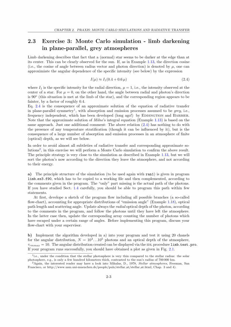
b) Implement the algorithm developed in a) into your program and test it using 20 chanelsfor the angular distribution, N = 104. . .105 photons and an optical depth of the atmosphere,τrmmax = 10. The angular distribution created can be displayed via the idl procedure limb test.pro.If your program runs successfully, you should have obtained a plot as given in Fig. 2.1.
1i.e., under the condition that the stellar photosphere is very thin compared to the stellar radius: the solarphotosphere, e.g., is only a few hundred kilometers thick, contrasted to the sun’s radius of 700 000 km.
2Again, the interested reader may have a look into Mihalas, D., 1978, Stellar atmospheres, Freeman, SanFrancisco, or http://www.usm.uni-muenchen.de/people/puls/stellar at/stellar at.html, Chap. 3 and 4).
2-3

CHAPTER 2. PRAXIS: MONTE CARLO SIMULATIONS AND RADIATIVE TRANSFER
Figure 2.1: Monte Carlo simulation of limb darkening: angular distribution of 105 photons sorted into 20channels. The total optical depth of the atmosphere is 10.
c) In our simulation, we have calculated the number of photons leaving the atmosphere withrespect to a surface perpendicular to the radial direction. Without going into details, this numberis proportional to the specific intensity weighted with the projection angle µ, since the specificintensity, I(µ), is defined with respect to unit projected area. Thus,
N(µ)dµ ∝ I(µ)µdµ, (2.5)
and the intensity within dµ is obtained from the number of photons, divided by an appropriateaverage of µ, i.e., centered at the mid of the corresponding channel (already implemented intothe program output).
This relation is also the reason why the distribution of the photons’ “emission angles” at thelower boundary follows the pdf µdµ: for an isotropic radiation field, which is assumed to bepresent at the lowermost boundary, it is the specific intensity and not the photon number whichis uniformly distributed with respect to µ! Thus, in order to convert to photon numbers, we haveto draw the emission angles at the lower boundary from the pdf µdµ instead of dµ! Inside theatmosphere, on the other hand, the emission angle refers to the photons themselves and thus is(almost) isotropic, so that we have to draw from the pdf dµ.
Modify the plot routine limb test.pro in such a way as to display the specific intensity andcompare with the prediction (2.4). Use N = 106 photons for τmax = 10 now, and derive thelimb-darkening coefficients (in analogy to Eq. 2.4) from a linear regression to your results. Hint:use the idl-procedure poly fit, described in idlhelp. Why is a certain discrepancy betweensimulation and theory to be expected?
2-4

CHAPTER 2. PRAXIS: MONTE CARLO SIMULATIONS AND RADIATIVE TRANSFER
d) To convince yourself that limb-darkening is the consequence of a multitude of scatteringeffects, reduce τmax to a very small value. Which angular distribution do you expect now for thespecific intensity? Does your simulation verify your expectation?
2-5

Index
Gauss-distribution, 1-5Hopf-function, 1-27Kolmogoroff-Smirnov-test, 1-12Mersenne prime number, 1-8Milne’s integral equation, 1-26Pearson’s χ2, 1-11, 1-12Schrage’s multiplication, 1-8planck-function, 2-2stefan-boltzmann-law, 2-2thomson-scattering, 1-27von Neumann’s rejection method, 1-32RANDU , 1-14
cumulative probability distribution, 1-3
distributionexponential, 1-31normal, 1-31uniform, 1-3, 1-30
event, 1-1expectation value, 1-2exponential distribution, 1-31
graphical test of random numbers, 1-15
hit or miss method, 1-23hyper-surfaces, 1-15
importance sampling, 1-24integration
Monte Carlo, 1-19intensity
specific, 2-2inversion method, 1-29
limb darkening, 2-3
Monte Carlo approximation, 1-19Monte Carlo integration, 1-19
cooking recipe, 1-21hit or miss, 1-23
method, 1-19scaling law for errors, 1-22
Monte Carlo simulations, 1-26more-dimensional tests of random numbers,
1-13
normal distribution, 1-5, 1-31
optical depth, 1-26
probability, 1-1probability density function, 1-2probability distribution
cumulative, 1-3pseudo random numbers, 1-6
random number generatorlinear congruential, 1-6minimum-standard, 1-8
random numbers, 1-6graphical test, 1-15more-dimensional tests, 1-13pseudo-, 1-6real, 1-6sub-, 1-6tests, 1-12
random variables, 1-1continuous, 1-2discrete, 1-1
rejection method, 1-32reshuffling, 1-16
specific intensity, 2-2standard deviation, 1-2stratified sampling, 1-24sub-random numbers, 1-6
tests of random numbers, 1-12transformation method, 1-29
uniform distribution, 1-3, 1-30
2-6

INDEX
variance, 1-2variance reduction, 1-24variate, 1-1
2-7