LTCC course on Potential Theory, Spring 2011

Boris Khoruzhenko1, QMUL

Contents (five two-hour lectures):

1. Harmonic functions: basic properties, maximum principle, mean-valueproperty, positive harmonic functions, Harnack’s Theorem

2. Subharmonic functions: maximum principle, local integrability

3. Potentials, polar sets, equilibrium measures

4. Dirichlet problem, harmonic measure

5. Capacity, transfinite diameter

The four lectures follow closely a textbook on Potential Theory in the Com-plex Plane by T. Ransford, apart from material on harmonic measure whichhas been borrowed from a lecture course Introduction to Potential Theorywith Applications, by C. Kuehn. The material in lecture 5 is borrowed froma survey Logarithmic Potential Theory with Applications to ApproximationTheory by E. B. Saff (E-print: arXiv:1010.3760).

1 Harmonic Functions

(Lecture notes for Day 1, 21 Feb 2011, revised 24 Feb 2011)

1.1 Harmonic and holomorphic functions

Let D be domain (connected open set) in C. We shall consider complex-valued and real valued functions of z = x + iy ∈ D. We shall write h(z) oroften simply h to denote both a function of complex z and a function in twovariables x and y.

Notation: hx will be used to denote the partial derivative of h with respectto variable x, similarly hxx, hyy, hxy and hyx are the second order partialderivatives of f .

Here come our main definition of the day. Recall that C2(D) denotes thespace of functions on D with continuous second order derivatives.

1E-mail: b.khoruzhenko@qmul.ac.uk, URL: http://maths.qmul.ac.uk\ ∼boris

1

Definition A function h : D → R is called harmonic on D if h ∈ C2(D) andhxx + hyy = 0 on D.

Examples(a) h(z) = |z|2 = x2 + y2 is not harmonic anywhere on C as hxx + hyy=2.

(b) h(z) = ln(|z|2) is harmonic on D = C\{0}. Indeed,

ln |z| = ln√x2 + y2 and (hxx + hyy)(z) = 0 if z 6= 0.

(c) h(z) = Re z = x2 − y2 is harmonic on C.

Recall that a complex-valued function f is called holomorphic on a do-main D if it is complex differentiable in a neighbourhood of any point inD. The existence of a complex derivative is a very strong condition: holo-morphic functions are actually infinitely differentiable and are representedby their own Taylor series. For a function f(z) = h(z) + ik(z) to be homo-morphic the following conditions are necessary and sufficient

Cauchy-Riemann equations: hx = ky and hy = −kx

Thm 1. Let D be a domain in C. If f is holomorphic on D then h = Re fis harmonic on D.

Proof. This follows from the Cauchy-Riemann equations.

The converse is also true but only for simply connected domains D, i.e.when every path between two arbitrary points in D can be continuouslytransformed, staying within D, into every other with the two endpoints stay-ing put.

Thm 2. If h is harmonic on D and D is simply-connected then h = Re ffor some holomorphic function f on D. This function is unique up to anadditive constant.

Proof. We first settle the issue of uniqueness. If h = Re f for some holomor-phic f , say f = h+ ik., then by the Cauchy-Riemann,

f ′ = hx + ikx = hy − ihy . (1.1)

Hence, if such f exists, then it is completely determined by the first orderderivatives of h, and, therefore, is unique up to an additive constant.

Equation (1.1) also suggest a way to construct the desired f . Defineg = hy − ihy. Then g ∈ C(D) and g satisfies the Cauchy-Riemann equa-tions because hxx = −hyy (h is harmonic) and hxy = hyx. Therefore g is

2

holomorphic in D. Now fix z0 ∈ D, and define f to be the anti-derivative ofg:

f(z) = h(z0) +

∫ z

z0

g(z)dz ,

with the integral being along a path in D connecting z and z0. As D is simplyconnected, Cauchy’s theorem asserts that the integral does not depend onthe choice of path. By construction, f is holomorphic and

f ′ = g = hx − ihy .

Writing h = Re f , by the Cauchy-Riemann for f ,

f ′ = hx − ihy.

On comparing the two equations, one concludes that hx = hx and hy = hy.Therefore h− h is a constant. Since h and h are equal at z0, they are equalthroughout.

One corollary of these theorems is that every harmonic function is differ-entiable infinitely many times.

Corollary 3. If h is a harmonic function on a domain D, then f ∈ C∞(D).

Another important corollary of Thm 2 is a property of harmonic functionsthat will be later used to define the important class of subharmonic functions.

Let ∆(w, r) denote the disk of radius r about w, and ∆(w, r) denote itsclosure,

∆(w, r) = {z : |w − z| < r} , ∆(w, r) = {z : |w − z| ≤ r} .

The boundary ∂∆ of ∆(w, r) is the set

∂∆(w, r) = {z : z = w + reiθ, θ ∈ [0, 2π)} .

Thm 4. (Mean-Value Property) Let h be a function harmonic in an openneighbourhood of the disk ∆(w, r). Then

h(w) =1

2π

∫ 2π

0

h(w + reiθ)dθ .

3

Proof. Function h is harmonic on ∆(w, ρ) for some ρ > r. By Thm 2 thereexists a function f which is holomorphic on ∆(w, ρ) and such that h = Re f .By Cauchy’s integral formula for f ,

f(w) =1

2πi

∮|z−w|=r

f(z)

z − wdz .

Introducing the parametrisation z = w + reiθ for the integration path above(θ runs from 0 to 2π), with dz = ireiθdθ, one arrives at

f(w) =1

2π

∫ 2π

0

f(w + reiθ) .

The result now follows on taking the real parts of both sides.

Recall that every holomorphic function is completely determined on adomain by its values in a neighbourhood of a single point. A similar propertyholds for harmonic functions.

Thm 5. (Identity Principle) Let h be a harmonic function on a domain Din C. If h = 0 on a non-empty open subset U of D then h = 0 throughoutD.

Proof. Set g = hx − ihy. Then as in the proof of Thm 2, g is holomorphicin D. Since h = 0 on U then so is g. Hence, by the Identity Principle forthe holomorphic functions g = 0 on D, and consequently, hx = hy = 0 onD. Therefore h is constant on D, and as it is zero on U , it must be zero onD.

Note that for the holomorphic functions a stronger identity principleholds: if f is holomorphic on D and vanishes on D at infinite number ofpoints which have a limiting point in D, then f vanish on D throughout.This is not the case for harmonic functions, e.g. the harmonic functionh = Re z vanishes on the imaginary axis, and only there.

The theorem below asserts that harmonic functions do not have localmaxima or minima on open sets U unless they are constant. Moreover, ifa harmonic function is negative (positive) on the boundary of an open U itwill be negative (positive) throughout U .

Thm 6. (Maximum Principle) Let h be a harmonic function on a domainD in C.

(a) If h attains a local maximum in D then h is constant.

4

(b) Suppose that D is bounded and h extends continuously to the boundary∂D of D. If h ≤ 0 on ∂D then h ≤ 0 throughout D.

Proof. Suppose that h attains a local maximum in D. Then there exists aopen disk ∆ such that h ≤ M in ∆ for some M . Consider the set K ={z ∈ ∆ : h(z) = M}. Since h is continuous, K is closed in ∆, as the set ofpoints where a continuous function takes a given value is closed. It is alsonon-empty. Suppose there exists a boundary point ζ of K in ∆. As K isclosed, h(ζ) = M , and, as ∆ is open, one can find a disk ∆(ζ, ρ) of radiusρ about ζ such that ∆(ζ, ρ) ⊂ ∆. There exist points on the circumferenceof ∆(ζ, ρ) where h < M (for if not, then ζ would not be at the boundary ofK). Let ζ + ρeiθ0 be one such point. Since the complement of K is an openset, there exists a neighbourhood of ζ + ρeiθ0 where h < M . Therefore onecan find ε > 0 and δ > 0 such that for all θ such that |θ − θ0| < δ:

h(ζ + ρeiθ) < M − ε . (1.2)

Now, write the mean-value property for h at point ζ,

h(ζ) =1

2π

∫ 2π

0

h(ζ + ρeiθ)dθ

=1

2π

∫|θ−θ0|<δ

h(ζ + ρeiθ)dθ +1

2π

∫|θ−θ0|≥δ

h(ζ + ρeiθ)dθ

The first integral above is ≤ 2δ(M − ε) in view of (1.2) and the second≤ (2π − 2δ)M because h ≤M throughout ∆. Therefore one concludes that

h(ζ) <1

2π[2δ(M − ε) + (2π − 2δ)M ] < M ,

which is a contradiction as by the construction h(ζ) = M . Hence K = {z ∈∆ : h(z) = M} cannot have boundary points in ∆ and therefore K = ∆.Hence h is constant on ∆. Then, by the identity principle Thm 5, h isconstant on D, and Part (a) is proved.

To prove Part (b), observe that h is continuous on D by assumption.Since D is compact, then h must attain a (global) maximum at some pointw ∈ D. If w ∈ ∂D then h(w) ≤ 0 by assumption, and so h ≤ 0 on D. Ifw ∈ D then, by Part (a), h is constant on D. Hence, by continuation, h isconstant on D of which ∂D is a subset, so once again h ≤ 0.

It follows from the identity principle that if two harmonic functions coin-cide in a neighbourhood of a single point of a domain D then they coincide

5

everywhere in D. We shall now establish a stronger property. If two har-monic functions coincide on the boundary of a disk about a point in D thenthey coincide throughout D.

We first settle the issue of uniqueness in the case of the entire D. Thecorresponding statement is known as the Uniqueness Theorem

Thm 7. (Uniqueness Theorem) Let D be a domain in C and h1 and h2 aretwo harmonic functions that extend continuously to the boundary ∂D of D.If h1 = h2 on ∂D then these two functions are equal throughout D.

Proof. Consider the function h = h1−h2. This function is harmonic and, byconstruction, h = 0 on ∂D. Therefore, by the Maximum Principle (Thm 6)h ≤ 0 on D. Applying now the Maximum Principle to the function −h weconclude that h = 0 on D, hence h1 = h2 there.

By evoking the Identity Principle (Thm 6) one can make a stronger state-ment about uniqueness.

Corollary 8. Let D be a domain in C and z ∈ D. If h1 and h2 are twofunctions harmonic on D and such that h1 = h2 on the boundary of a diskabout z in D then these two functions are equal throughout D.

1.2 Poisson integral

Since the boundary values of harmonic function determine this functionuniquely (under the assumption of continuity on the boundary), it is nat-ural to ask the question about reconstructing the harmonic function from itsboundary values. A slightly more general problem is known as the DirichletProblem.

Definition Let D be a domain in C and let φ : ∂D → R be a continuousfunction . The Dirichlet problem is to find a function h harmonic on D andsuch that limz→ζ h(z) = φ(ζ) for all ζ ∈ D.

The uniqueness of solution of the Dirichlet Problem follows is asserted byThm 7. The question of existence is more delicate. We shall solve here oneimportant case of a circular domain (disk) when the positive answer comesvia an explicit construction. It uses the so-called Poisson Kernel.

Now we shall set about finding the harmonic function on a disk from itsvalues on the disk boundary.

6

Definition The following real-valued function of two complex variables zand ζ

P (z, ζ) = Re

(ζ + z

ζ − z

)=

1− |z|2

|ζ − z|2(|z| < 1, |ζ| = 1)

is known as the Poisson kernel.

Lemma 9. (Properties of the Poisson kernel)

(a) P (z, ζ) > 0 for |z| < 1 and |ζ| = 1;

(b) 12π

∫ 2π

0P (z, eiθ)dθ = 1;

(c) sup|ζ−ζ0|≥δ P (z, ζ)→ 0 as z → ζ0 (|ζ0| = 1 and δ > 0) .

Proof. Parts (a) and (c) are obvious (for part (c) observe that as z approachesζ0, the top of the fraction defining the Poisson kernel goes to zero and thebottom is bounded away from zero by the triangle inequality |z − ζ| ≥ |ζ −ζ0| − |z − ζ0|).

A calculation is required for Part (b) . Observe that

1

2π

∫ 2π

0

P (z, eiθ)dθ = Re

(1

2πi

∫|ζ|=1

ζ + z

ζ − zdζ

ζ

).

Sinceζ + z

(ζ − z)ζ=

2

ζ − z− 1

ζ,

Part (b) now follows from Cauchy’s integral formula

f(z) =1

2πi

∮f(ζ) dζ

ζ − z

for holomorphic functions.

The Poisson kernel is defined for z in the unit disk about the origin. Bymaking an affine change of variables u = z−w

ρone can map a disk about w of

radius ρ in z-plane to the unit disk about the origin in u-plane. This justifiesthe following definition.

Definition Let φ : ∆(w, ρ) → R be continuous function. Then its PoissonIntegral P∆φ is defined by

P∆φ(z) =1

2π

∫ 2π

0

P

(z − wρ

, eiθ)φ(w + ρeiθ)dθ (z ∈ ∆)

7

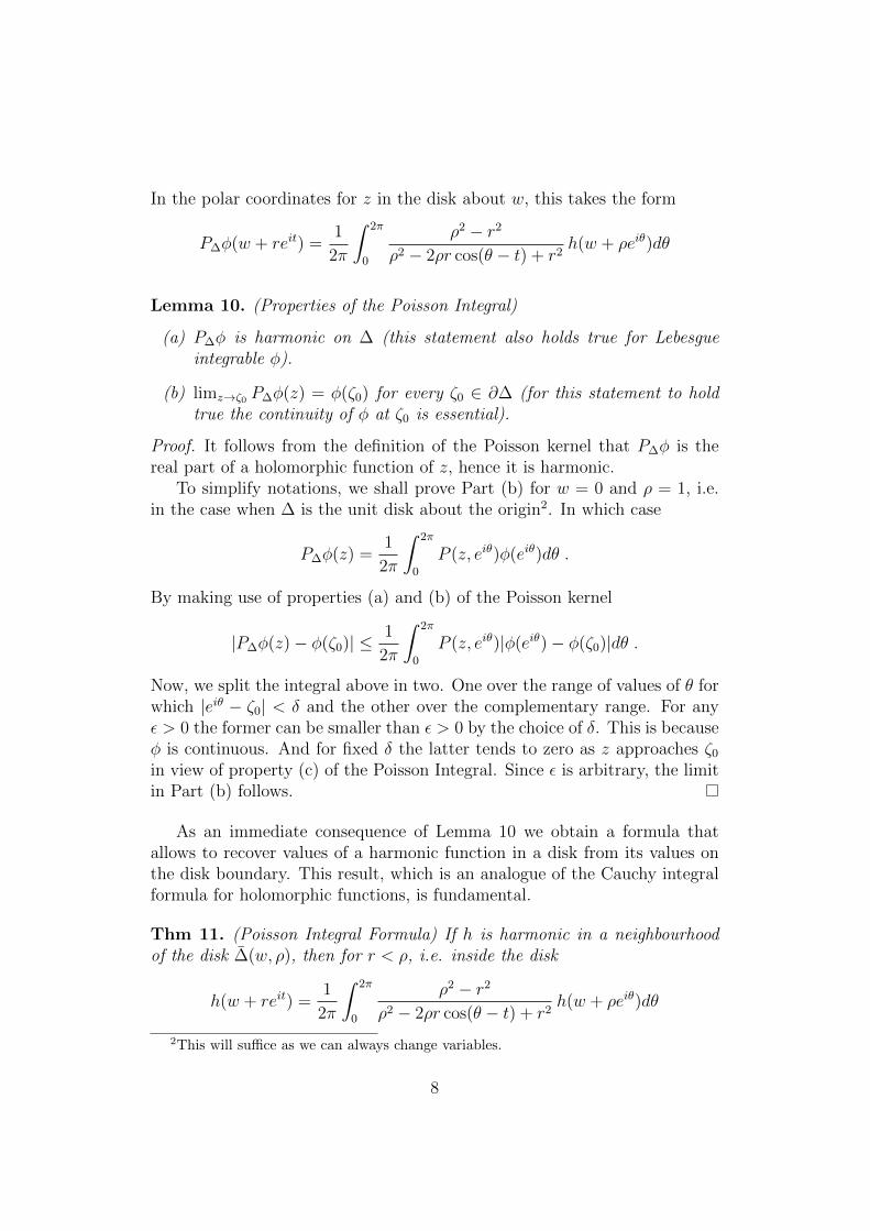
In the polar coordinates for z in the disk about w, this takes the form

P∆φ(w + reit) =1

2π

∫ 2π

0

ρ2 − r2

ρ2 − 2ρr cos(θ − t) + r2h(w + ρeiθ)dθ

Lemma 10. (Properties of the Poisson Integral)

(a) P∆φ is harmonic on ∆ (this statement also holds true for Lebesgueintegrable φ).

(b) limz→ζ0 P∆φ(z) = φ(ζ0) for every ζ0 ∈ ∂∆ (for this statement to holdtrue the continuity of φ at ζ0 is essential).

Proof. It follows from the definition of the Poisson kernel that P∆φ is thereal part of a holomorphic function of z, hence it is harmonic.

To simplify notations, we shall prove Part (b) for w = 0 and ρ = 1, i.e.in the case when ∆ is the unit disk about the origin2. In which case

P∆φ(z) =1

2π

∫ 2π

0

P (z, eiθ)φ(eiθ)dθ .

By making use of properties (a) and (b) of the Poisson kernel

|P∆φ(z)− φ(ζ0)| ≤ 1

2π

∫ 2π

0

P (z, eiθ)|φ(eiθ)− φ(ζ0)|dθ .

Now, we split the integral above in two. One over the range of values of θ forwhich |eiθ − ζ0| < δ and the other over the complementary range. For anyε > 0 the former can be smaller than ε > 0 by the choice of δ. This is becauseφ is continuous. And for fixed δ the latter tends to zero as z approaches ζ0

in view of property (c) of the Poisson Integral. Since ε is arbitrary, the limitin Part (b) follows.

As an immediate consequence of Lemma 10 we obtain a formula thatallows to recover values of a harmonic function in a disk from its values onthe disk boundary. This result, which is an analogue of the Cauchy integralformula for holomorphic functions, is fundamental.

Thm 11. (Poisson Integral Formula) If h is harmonic in a neighbourhoodof the disk ∆(w, ρ), then for r < ρ, i.e. inside the disk

h(w + reit) =1

2π

∫ 2π

0

ρ2 − r2

ρ2 − 2ρr cos(θ − t) + r2h(w + ρeiθ)dθ

2This will suffice as we can always change variables.

8

Proof. Since h is harmonic in a neighbourhood of ∆(w, ρ), it is continuous onthe boundary ∂∆. Denote its restriction to ∂∆ by φ, i.e., φ = h |∂∆ . Then,by Thm 11, P∆φ(z) is harmonic on ∆, extends continuously to the boundaryof ∆ and coincides there with h. Therefore, by the Uniqueness Theorem 8h = P∆φ.

Writing the Poisson Integral Formula in the centre of the disk, i.e. forr = 0, one recovers the Mean-Value Property of harmonic functions whichwe established earlier. Thus, the Poisson Integral Formula can be viewed asa generalisation of the Mean-Value Property.

1.3 Positive harmonic functions

The Poisson integral formula allows to obtain useful inequalities for positiveharmonic functions. Note that if a non-negative harmonic function attains aminimum value zero on a domain, it is zero throughout the domain. So theclass of non-negative harmonic functions on a domain consists of all positivefunctions and a zero function.

Thm 12. (Harnack’s Inequality) Let h be a positive harmonic function onthe disk ∆(w, ρ) of radius ρ about w. Then for r < ρ and all t

ρ− rρ+ r

h(w) ≤ h(w + reit) ≤ ρ+ r

ρ− rh(w)

i.e. the values of h in the disk ∆(w, ρ) are bounded below and above bymultiples of the value of h at the centre w of the disk, with both bounds onlydepending on the distance to the centre.

Proof. Choose any s such that r < s < ρ and apply the Poisson integralformula to to h on ∆(w, s). As h is positive, we have

h(w + reit) =1

2π

∫ 2π

0

s2 − r2

s2 − 2sr cos(θ − t) + r2h(w + seiθ)dθ

≤ 1

2π

∫ 2π

0

s2 − r2

(s− r)2h(w + seiθ)dθ .

Simplifying the fraction and applying the mean-value property one obtainsthe desired upper bound. The lower bound is proved similarly.

Recall that any function that is holomorphic on C and bounded in abso-lute value is a constant. As an immediate corollary of Harnack’s inequalitiesone obtains an analogue of this result for harmonic functions.

9

Corollary 13. (Liouville Theorem) Every harmonic function on C that isbounded below or above is constant.

Proof. It will suffice to show that every positive harmonic function on C isconstant. Let h be positive and harmonic on C. By Harnack’s inequalitiesapplied for ∆(0, ρ),

h(z) ≤ ρ+ |z|ρ− |z|

h(0) .

Letting ρ→∞ and keeping z fixed, one concludes that h(z) ≤ h(0) for anyz ∈ C, hence h attains a maximum at 0. The Maximum Principle (Thm 7)then implies that h must be constant.

Harnack’s inequality on disks extends to general domains and can be usedto define a distance between two points.

Corollary 14. Let D be a domain in C and z, w ∈ C. Then there exists anumber τ such that, for every positive harmonic function on D,

τ−1h(w) ≤ h(z) ≤ τ h(w) . (1.3)

Proof. Given z, w we shall write z ∼ w if there exists τ such that (1.3)holds for all positive functions harmonic on D. It is apparent that ∼is anequivalence relation. That is, (i) z ∼ z; (ii) if z ∼ w then w ∼ z; and (iii)if z ∼ w and w ∼ u then z ∼ u. Consider the corresponding equivalenceclasses. By the Harnack’s inequality they are open sets. As D is connected,there can only be one such equivalence class, hence (1.3) holds for all z, w.

Definition (Harnack Distance) Let D be a domain in C. Given z, w ∈ D,the Harnack distance between z and w is the smallest number τD(z, w) suchthat for every positive harmonic function h on D

τD(z, w)−1h(w) ≤ h(z) ≤ τD(z, w)h(w) .

The Harnack distance is an useful notion and can be used to deduce animportant theorem about convergence of positive harmonic functions, below.However, we do not have time to discuss it in detail. Instead we just statetwo of its properties.

Lemma 15. (Properties of the Harnack Distance)

(a) If D1 ⊂ D2 then τD2(z, w) ≤ τD1(z, w) for all z, w ∈ D1.

(b) If D is a subdomain of C then ln τD(z, w) is a continuous semi-metricon D (continuity meaning that ln τD(z, w)→ 0 as z → w).

10

We shall finish this section with several important results about conver-gence of a sequence of harmonic functions. Proofs are not given here and canbe found in Ransford’s book.

Firstly, local uniform convergence of harmonic functions implies that thelimiting function is also harmonic.

Thm 16. If (hn)n≥1 is a sequence of harmonic functions on a domain Dconverging locally uniformly to a function h, then h is also harmonic on D.

Non-increasing sequences of harmonic functions always converge (locallyuniformly), a result known as Harnack’s theorem.

Thm 17. (Harnack’s Theorem) Let (hn)n≥1 be non-decreasing sequence ofharmonic functions on a domain D, i.e., h1 ≤ h2 ≤ h3 ≤ . . .. Then eitherhn → ∞ locally uniformly, or else hn → h locally uniformly, where h isharmonic.

For positive sequences of harmonic functions one can only guarantee con-vergence of a subsequence.

Thm 18. Let (hn)n≥1 be a sequence of positive harmonic functions on adomain D. Then either hn →∞ locally uniformly, or else some subsequencehnj→ h locally uniformly, where h is harmonic.

Exercises 1

(1.1a) Show that the Poisson kernel is given by

P (reit, eiθ) =+∞∑

n=−∞

r|n|ein(t−θ) (r < 1, 0 ≤ t, θ < 2π) .

Use this to derive an alternative proof if Lemma 9 (b).

(1.1b) Show that it φ : ∂∆(0, 1)→ R is an integrable function, then

P∆φ(reit) =+∞∑

n=−∞

anr|n|eint (r < 1, 0 ≤ t < 2π) ,

where (an)n is a bounded sequence of real numbers.

11

(1.1c) Assume now that φ is continuous. Writing φr(eit) = P∆φ(reit), show

that φr → φ uniformly on the unit circle as r → 1, and deduce thatφ(eit) can be uniformly approximated by trigonometric polynomials∑N

n=−N bbeint.

1.2 (Harnack distance) Let ∆ = ∆(w, 1). Show that

τ∆ =1 + |z − w|1− |z − w|

(z ∈ ∆) .

Hint: Use Harnack’s inequality to establish an upper bound and thenshow that this bound is attained on the positive harmonic functionh(z) = P (z − w, ζ).

12

2 Subharmonic Functions

(Notes for Day 2, 28 Feb 2011)

There are two standard approaches to define subharmonic functions. Oneis to require that uxx + uyy ≥ 0 in the sense of distribution theory, matchingthe characteristic property of the harmonic functions. And the other oneis via a submean property, matching the mean value property of harmonicfunctions. We shall follow the second approach.

Recall that the harmonic functions are continuous. However, subhar-monic functions are not required to be continuous. For if they were thatwould be too restrictive as continuity is not preserved when taking limits offunctions with uxx + uyy ≥ 0. Obviously, one need to require some kind ofregularity to have a meaningful theory, and it appears that semicontinuitysuffices.

2.1 Upper semicontinuous functions

Recall that a function f on a metric space X is called continuous at x if forany given positive ε one can find a open ball ∆(x, δ) of radius δ about x,∆(x, δ) = {y : dist(x, y, ) < δ}, such that

f(x)− ε ≤ f(y) ≤ f(x) + ε (z ∈ ∆(x, δ)) .

The inequality above is two-sided. If only one-sided inequality holds thenthe function is said to be semi-continuous.

Definition (Upper semi-continuity) A function f : X → [−∞,+∞) is calledupper semi-continuous at x ∈ X if for any given positive ε one can find apositive δ such that

f(y) ≤ f(x) + ε (y ∈ ∆(x, δ)) .

Note that upper semi-continuous functions are allowed to take value −∞.This is consistent with the definition above.

A function f is said to be upper semi-continuous on X if it has thisproperty at every x ∈ X. An equivalent definition for f to be upper semi-continuous on X is to require that

lim supy→x

f(y) ≤ f(x) (x ∈ X) . (2.1)

Yet another equivalent definition is to require the sets {x ∈ D : f(x) < α}be open in D for every α ∈ R.

13

Obviously, every continuous function is also upper semi-continuous. Be-low are a few examples of functions that are upper semi-continuous but notcontinuous.

Examples(a) f(z) = ln |z|, z ∈ C. f is not continuous at z = 0.

(b) f(x) = |x| if x 6= 0 and f(0) = 1 (x real or complex).

(c) f(x) = sin(1/x) if x 6= 0 and f(0) = 1.

(d) The characteristic function of a closed set in D.

Obviously, if f and g are upper semi-continuous functions, so is their sumf + g and max(f(z), g(z)).

Thm 19. Let f be upper semi-continuous. Then f is bounded above oncompact sets and attains its upper bound in every compact set.

Proof. Based on the Bolzano-Weierstrass theorem and is same as for con-tinuous functions. Let M = supx∈K f(x), where M may be +∞. By thedefinition of sup, there exists a sequence (xn) such that f(xn) → M asn → ∞. If K is compact then (xn) contains a subsequence converging to apoint x ∈ K. It follows from (2.1) that M ≤ f(x), hence M is finite. Alsosince f(x) ≤M on K, one concludes that f(x) = M .

Thm 20. (Monotone Approximation by Continuous Majorants) If f is up-per semi-continuous and bounded above on X then sequence of continuousfunctions (fn such that f1 ≥ f2 ≥ f3 ≥ . . . ≥ f and f = limn→∞ fn on X.The convergence is pointwise.

Proof. In the singular case when f = −∞ we can simply take fn = −n.Suppose now that f 6≡ −∞. Define

fn(x) = supy∈D

(f(y)− n dist(y, x)) .

Obviously fn ≥ fn+1 and fn ≥ f for every n. These functions also satisfythe inequality

fn(x) ≤ fn(w) + n dist(x,w) (x,w ∈ X) , (2.2)

from which it follows that fn is continuous on X for every n. For, interchang-ing x and w one gets |f(x)− f(w)| ≤ dist(x,w).

14

To prove (2.2), let us fix w. By definition of fn, for every ε > 0 thereexists yε such that

fn(w)− ε ≤ f(yε)− n dist(yε, w) ≤ fn(w) . (2.3)

Now,

fn(x) ≥ f(yε)− n dist(yε, x)

= f(yε)− n dist(yε, w) + n dist(yε, w)− n dist(yε, x)

≥ fn(w)− ε− dist(x,w) ,

where on the last step we have used (2.3) and the triangle inequality dist(yε, w) ≤dist(yε, x) + dist(x,w). Therefore for every ε > 0,

fn(w) ≤ fn(x) + dist(x,w) + ε .

By letting ε→ 0, one obtains (2.2). So fn are continuous.It remains to prove that fn converge to f . Fix x. By definition of fn, for

every n, we can find xn such

fn(x)− 1

n≤ f(xn)− n dist(xn, x) . (2.4)

After rearranging for dist(xn, x):,

n dist(xn, x) ≤ 1

n− fn(x) + f(xn) ≤ 1− f(x) + sup

x∈Xf(x) .

As f is bounded above, it follows that xn → x as n → ∞. Letting n → ∞in (2.4), and making use of (2.1),

limn→∞

fn(x) ≤ lim supn→∞

f(xn) ≤ f(x) .

On the other hand, limn→∞ fn(x) ≥ f(x) because fn(x) ≥ f(x) for every n.Hence limn→∞ fn(x) ≥ f(x), and theorem follows.

2.2 Subharmonic functions and their properties

Definition (Subharmonic Functions). Let U be an open subset of C. Afunction u is called subharmonic is u is upper semi-continuous and satisfiesthe local submean inequality. Namely, for any w ∈ U there exists ρ > 0 suchthat

u(w) ≤ 1

2π

∫ 2π

0

u(w + ρeit)dt (0 ≤ r < ρ) . (2.5)

15

Note, that according to this definition u ≡ −∞ is a subharmonic function.

The integral in (2.5) is understood as the Lebesgue integral and is welldefined for upper semi-continuous functions. Indeed,

∫u =

∫u+ −

∫u−,

where u± = max(±u, 0). By Thm 19 , u+ is bounded. Thus if∫u− is finite

then the whole integral is finite too. If∫u− = +∞ then the whole integral∫

u = −∞. We shall see later (Corollary 28) that the latter can only happenonly if u ≡ −∞.

The following theorem provides an important example of subharmonicfunction.

Thm 21. If f is holomorphic on D then ln |f | is subharmonic on D.

Proof. ln |f | is upper semi-continuous, so one only needs to verify the localsub-mean property. Consider a point w ∈ D. If f(w) 6= 0, then ln |f | isharmonic near w and hence (2.5) follows from the mean value property ofharmonic functions. If f(w) = 0 then ln |f(w)| = −∞ and (2.5) is satisfiedanyway.

Note that if u and v are subharmonic then so is αu+ βv for all α, β ≥ 0,as well as max(u, v).

The following result is central and is an extension of the correspondingproperty of the harmonic functions to subharmonic functions (however, spotthe differences ...)

Thm 22. (Maximum Principle) Let u be subharmonic on a domain D in C.

(a) If u attains a global maximum in D then u is constant.

(b) If D is bounded and lim supz→ζ

u(z) ≤ 0 for all ζ ∈ ∂D, then u ≤ 0 on D.

Proof. Suppose that u attains a maximum value of M on D. Define

A = {z ∈ D : u(z) < M}, K = {z ∈ D : u(z) = M} .

The set A open because u is upper semi-continuous. The set K is opentoo because of the local submean property for subharmonic functions (anysufficiently small circle about z ∈ K must lie in K, for if not then there is acircle that intersects with A, and since A is open the intersection will containa segment of finite length hence the mean value integral will be < 2πM inviolation of the local submean property). By assumption, A and K partitionD. Since D is connected, one of the two sets must be empty. The set K isnon-empty by assumption, therefore A = ∅, and Part (a) is proved.

16

To prove part (b), let us extend u to the boundary of D by u(ζ) =lim supz→ζ u(z), for ζ ∈ ∂D. Then u is upper semi-continuous on D. SinceD is compact by Thm 19) u attains a maximum on D. If the maximumpoint is in D, then u = 0 on D by Part (a). If the maximum point is at theboundary of D then u ≤ 0 on D.

Comparison to the maximum principle for harmonic functions:

- local max for harmonic, global for subharmonic

- min or max for harmonic functions, only max for subharmonic

The subharmonic function u = max(Re z, 0) attains a local maximumand a global minimum but is not constant.

The following theorem explains the name for subharmonic functions.

Thm 23. (Harmonic Majoration) Let D be a bounded domain in C andsuppose that u is subharmonic in D and h is harmonic there. Then

‘ lim supz→ζ

(u− h)(z) ≤ 0 for all ζ ∈ ∂D′ =⇒ ‘u ≤ h on D’ . (2.6)

Proof. The function u− h is subharmonic, hence the result follows from themaximum principle for subharmonic functions, Part (b) of Thm 22.

Recall that harmonic functions can be represented via the Poisson integralformula. Correspondingly, subharmonic functions are bounded from aboveby the Poisson integral (you might expected this coming ...)

Thm 24. (Poisson Integral Inequality) If u is subharmonic in a neighbour-hood of ∆(w, ρ) then for r < ρ

u(w + reit) ≤ 1

2π

∫ 2π

0

ρ2 − r2

ρ2 − 2ρr cos(θ − t) + r2u(w + ρeiθ)dθ . (2.7)

Proof. By Thm 20, there are continuous functions φn : ∂∆ → R such thatφn ↓ u on ∂∆. Since φn is continuous, the function P∆φn is harmonic andlimz→ζ(P∆φn)(z) → φn(ζ) for ζ ∈ ∂D. Hence, (recall that φn ≥ u for everyn)

lim supz→ζ

(u− P∆φn) ≤ u− φn ≤ 0 .

Therefore, by the harmonic majoration theorem, Thm 23, u ≤ P∆φn on ∆.Letting n → ∞ and using the monotone convergence theorem for Lebesgueintegrals gives the desired inequality.

17

As an immediate consequence of the Poisson integral inequality (put r = 0in (2.7), one concludes that subharmonic functions satisfy the global submeaninequality.

Corollary 25. (Global Submean Inequality) If u is subharmonic on an openset U and ∆(w, ρ) ∈ U then

u(w) ≤ 1

2π

∫ 2π

0

u(w + ρeit)dt .

Observe that (2.7) implies the local submean inequality (2.5), so we havea sequence of implications

(2.5) =⇒ (2.6) for all harmonic h =⇒ (2.7) =⇒ (2.5),

thus for upper semi-continuous functions any of (2.5)-(2.7) can be used asa criterion for subharmonicity. By making use of the criterion ’(2.6)for all harmonic h’ Ransford proves that u ∈ C2(U) is subharmonic if andonly if hxx + hyy ≥ 0.

The following limit theorem for decreasing sequences of of subharmonicfunctions is simple but useful.

Thm 26. Let (un)n be subharmonic functions on an open set U in C andsuppose that u≥u2 ≥ u3 ≥ . . . on U . Then u := limn→∞ un is subharmonic.

Proof. For each α ∈ R the set {z : u(z) < α} is the union of the open sets{z : un(z) < α}, so it is open too and hence u is upper semi-continuous.

If ∆(w, ρ) ∈ U then the global submean inequality for un ensures

un(w) ≤ 1

2π

∫ 2π

0

un(w + ρeit)dt .

for all n. Letting n → ∞ and applying the monotone convergence theoremon deduces that u satisfies the submean inequality, hence is subharmonic.

2.3 Integrability of subharmonic functions

Subharmonic functions are bounded above on compact sets but can be un-bounded below. This poses the natural question about their integrability.The answer tuns out to be positive, subharmonic functions are locally inte-grable, implying that they cannot be ‘too unbounded’.

Thm 27. (Local Integrability) Let u be subharmonic on a domain D in Csuch that u 6= −∞ identically on D. Then u is locally integrable.

18

Proof. One has to verify that for every w ∈ D∫∆(w,ρ)

|u(z)|d2z <∞ for some ρ > 0 , (2.8)

where d2z = dxdy is the element of area in the complex plane. Let A bethe set of w possessing this property and B be its complement in D. Thestrategy of proof is to show that both A and B are open, and that u = −∞on B. This will imply that D = A and B = ∅ since D is connected andu 6≡ −∞ on D.

A is open: Let w ∈ A so that (2.8) holds. Then every z ∈ ∆(w, ρ) belongsto A as well. For, ∆(z, r) ⊂ ∆(w, ρ) for sufficiently small r, and hence theintegral of |u| over ∆(z, r) is finite too.

B is open: Let w ∈ B and choose ρ such that ∆(w, 2ρ) ⊂ D. Then,because w ∈ B, ∫

∆(w,ρ)

|u(z)| d2z =∞ .

Given w′ ∈ ∆(w, ρ) set ρ′ = ρ + |w′ − w|. The disk about w′ of radius ρ′

covers ∆(w, ρ), hence ∫∆(w′,ρ′)

|u(z)| d2z =∞ .

As u is bounded above on compact sets, this implies that∫∆(w′,ρ′)

u(z) d2z = −∞ .

By the submean inequality at w′,

πρ′2u(w′) ≤∫ ρ′

0

(∫ 2π

0

u(w′ + reit)dt

)r dr =

∫∆(w′,ρ′)

u(z) d2z = −∞ .

(As u is bounded above on ∆(w′, ρ′) , the repeated integral coincides withthe double integral). Hence u = infty on ∆(w, ρ). This implies that B isopen and u = −∞ on B.

By the compactness argument, local integrability implies integrability oncompact sets. This implies integrability on circles.

Corollary 28. Let u subharmonic on a domain D and u 6≡ −∞ there. Then∫ 2π

0

u(w + ρeit)dt > −∞ (∆(w, ρ) ⊂ U) .

19

Proof. We may assume that u ≤ 0 on D (recall that u is bounded on compactsets). Then by the Poisson integral inequality, Thm 24, for any r < ρ,

u(w + reit) ≤ 1

2π

∫ 2π

0

ρ2 − r2

ρ2 − 2ρr cos(θ − t) + r2u(w + ρeiθ)dθ

≤ ρ− rρ+ r

1

2π

∫ 2π

0

u(w + ρeiθ)dθ .

Suppose that∫ 2π

0u(w+ ρeit)dt = −∞. Then the last inequality implies that

u = −∞ on ∆(w, ρ), and, consequently, u is not integrable. This contradictsThm 27, hence the integral above is finite.

By a standard measure theory argument, integrability on compact setsimplies that the set of points in C where a subharmonic function takes value−∞ has Lebesgue measure zero.

2.4 Three theorems not covered but useful (of coursethere are many more ....)

Thm 29. Let U be an open subset of C, and u ∈ C2(U). Then u is subhar-monic on U if and only if uxx + uyy ≥ 0.

Thm 30. (Liouville Theorem) Let u be subharmonic on C such that

lim supz→∞

u(z)

ln |z|≤ 0 .

Then u is constant on C. E.g., every subharmonic function on C which isbounded above must be constant.

Thm 31. (Weak Identity Principle) Let u v be subharmonic on an open setU in C. If u = v almost everywhere on U then u = v everywhere on C. E.g.,if two subharmonic functions coincide off the real line, they coincide on thereal line too!

2.5 Two topics not covered but important

There are strong similarities between subharmonic functions and convex func-tions on R. More on this in Ransford’s book, and also in Notions of Convexityby Lars Hormander.

20

We also had no time to time to study the important technique of smooth-ing, mightn need to come back to this one later.

Exercises 2

(1) By making use of the integral

1

2π

∫ 2π

0

ln |reit − ζ| dt =

{ln |ζ|, if r ≤ |ζ|,ln r, if r > |ζ|,

show that the function u(z) =∞∑n=1

2−n ln |z − 2−n| is subharmonic.

(2a) Suppose that (un) is sequence of subharmonic functions on C such thatsupn un is bounded above on compact sets. Let u =

∑∞n=1 αnun, where

αn ≥ 0 and∑∞

n=1 αn <∞. Prove that u is upper semi-continuous andsatisfies the local submean inequality, hence, is subharmonic.

[Hint: Upper semi-continuity follows from Fatou’s Lemma. ]

(2b) Let (wn) be a countable dense subset of the unit disk ∆(0, 1) in thecomplex plane. Define u(z) =

∑∞n=1 2−n ln |z−wn|. It follows from (2a)

that u is subharmonic. Prove that u is discontinuous almost everywherein ∆(0, 1).

[Hint: Consider the set E = {z : u(z) = −∞} ⊂ C. The function u isdiscontinuous at every point in E\E.]

3 Let u be a subharmonic function on ∆(0, 1) such that u < 0. Provethat for every ζ ∈ ∂∆(0, 1),

lim supr→1−

u(rζ)

1− r< 0

[Hint: Apply the maximum principle to u(z) + c ln |z| on the annulus0.5 < |z| < 1 for a suitable constant c. ]

21

(Notes for Day 3, 7 March 2011)

3 Potentials and Generalised Laplacian

We shall only consider potentials of finite measures with compact support inC. This captures the essence but avoids technicalities.

The measures we consider are Borel measures, i.e. positive measures onthe Borel σ algebra of open sets in C. The support suppµ of measure µ isthe (closed) set of all z ∈ C such that µ(∆(z, r)) > 0 for any r > 0.

Definition (Logarithmic Potential) Let µ be a finite mass Borel measure onC with compact support. Its potential pµ is the function

pµ(z) =

∫C

ln |z − w| dµ(w) (z ∈ C).

Thm 32. pµ is subharmonic on C and harmonic on C\(suppµ).

Proof. Let K be the support of µ. Since K is compact, the function fz(w) =ln |z − w| is bounded above on K. It then follows that pµ(z) is upper semi-continuous (by Fatou’s Lemma), and has the submean property (by FubiniTheorem and subharmonicity of ln |z|). Hence pµ(z) is subharmonic on C.

As K is closed, C\K is open. Hence pµ(z) is harmonic on C\K, e.g., bydirect computation.

Note that the log-potential is some time defined as∫C ln(1/|z−w|) dµ(w),

so that it is superharmonic function (lower semi-conitinuous and the inequal-ity in the submean property in the other direction. This corresponds betterto the real word, where the electric potential created by a point charge qat distance r from the charge is proportional to qrd−2 in d-dimensions wordand to q ln(1/r) in two dimensions. Correspondingly, the potential due to acharge distribution ρ(w) will be given by

∫C ln(1/|z − w|) ρ(w)d2w.

Thm 33. (Continuity at Boundary of Support) Let µ be a finite Borel mea-sure with compact support K and ζ0 ∈ ∂K. Then

lim infz→ζ0

pµ(z) = lim infζ→ζ0, ζ∈K

pµ(ζ) . (3.1)

Furthermore,

if limζ→ζ0, ζ∈K

pµ(z) = pµ(ζ0) then limz→ζ0

pµ(z) = pµ(ζ0) . (3.2)

22

Proof. If pµ(ζ0) = −∞ then limz→ζ0 pµ(z) = −∞ by upper semi-continuity,and (3.1) holds.

Suppose now that pµ(ζ0) > −∞. Then µ({ζ0}) = 0. Since µ(∩nAn) =limn→∞ µ(An), it then follows that for every ε > 0 there exists r > 0 suchthat µ(∆(ζ0, r)) < ε. By definition of lim sup,

lim infz→ζ0

pµ(z) ≤ lim infζ→ζ0, ζ∈K

pµ(ζ) ,

so to prove (3.1) it will suffice to prove the inequality in the opposite direction.For every z ∈ C choose ζz ∈ K that minimizes |z − ζ| over ζ ∈ K. Then

|ζz − w||z − w|

≤ |z − ζz|+ |z − w||z − w|

≤ 2 .

Therefore

pµ(z) ≥ pµ(ζz)− ε ln 2−∫K\∆(ζ0,r)

ln|ζz − w||z − w|

dµ(w) .

As z → ζ0 in C, the corresponding ζz → ζ0 in K, and, hence,

lim infz→ζ0

pµ(z) ≥ lim infζz→ζ0, ζ∈K

pµ(ζz)− ε ln 2 .

Be letting ε→ 0,

lim infz→ζ0

pµ(z) ≥ lim infζz→ζ0, ζ∈K

pµ(ζz) ≥ lim infζ→ζ0, ζ∈K

pµ(ζ) ,

which proves (3.1). In its turn, (3.1) and upper semi-continuity proves (3.2).

Thm 34. (Minimum Principle) Let µ be a finite Borel measure with compactsupport K.

If pµ ≥M on K then pµ ≥M on C.

Proof. The function u = −pµ(z) is subharmonic on C\K and u(z) → −∞as z → ∞. Then for all sufficiently large R > 0, u(R) ≤ −M . Applyingthe maximum principle for subharmonic functions to u and the domain D =∆(0, R)\K, one concludes that u(z) ≤ −M on D for all sufficiently large R,hence the theorem.

23

3.1 Polar Sets

Polar sets play the role of negligible sets in potential theory. To define polarsets, we need first to introduce the concept of energy associated with measure(actually, anti-energy, due to our choice of sign of the logarithmic potential,so that minimisation of physical energy would correspond to maximisationof I(µ) as defined below.)

Definition Let µ be a finite Borel measure with compact support. Its energyI(µ) is defined as

I(µ) =

∫pµdµ =

∫ ∫ln |z − w|dµ(z)dµ(w).

Since pµ is bounded above on compact sets, the above integral is well defined,and I(µ) < µ(K) supK pµ. However, it may happen that I(µ) = −∞. Forexample, the Dirac measure dµ = δz0 has potential ln |z− z0|, hence I(δz0) =−∞. Similarly, any measure supported by a finite or countable set hasinfinite energy. Sets supporting only measures of infinite energy, of which acountable set is an example, are called polar sets.

Definition (Polar Set) A subset E of C is called polar if I(µ) = −∞ forevery non-zero Borel measure µ of finite mass supported on a compact subsetof E.

The theorem below asserts that, in the language of electrostatics, boundedBorel polar can hold no charge.

Thm 35. Let µ be a finite Borel measure with compact support and such thatI(µ) > −∞. Then µ(E) = 0 for every Borel polar set E.

Proof. Let E be a measurable set such that µ(E) > 0. By regularity of µ,one can choose a compact subset K ⊂ E such that µ(K) > 0. Set µ = µ |K .Then µ is a finite measure with support K. Set now d to be the diameter ofthe support of µ, so that ln |z−w|

d≤ 0 for all z, w ∈ suppµ. Then

I(µ) =

∫K

∫K

ln|z − w|d

dµ(z)dµ(w) + µ(K)2 ln 2

≥∫C

∫C

ln|z − w|d

dµ(z)dµ(w) + µ(K)2 ln 2

= I(µ)− µ(C)2 ln d+ µ(K)2 ln 2 > −∞ ,

so E cannot be polar.

Corollary 36. Every Borel polar set in C has 2D Lebesgue measure zero.

24

Proof. Let R > 0 and µ be the restriction the two-dimensional Lebesguemeasure to the disk ∆(0, R). Since ln |z| is locally integrable, its potentialpµ(z) =

∫∆(0,R)

ln |z−w|d2w > −∞, hence integrable on ∆(0, R) by the local

integrability theorem for subharmonic functions. This can also be checkeddirectly of course. Therefore, I(µ) > −∞ for every R. The assertion ofCorollary now follows from Thm 35 by letting R→∞.

A property is said to hold nearly everywhere (n.e.) on S ⊂ C if it holdson S\E for some Borel polar E. Thus ‘nearly everywhere’ implies almosteverywhere. The converse is false (e.g., the unit interval [0,1] has Lebesguemeasure zero but is not polar).

Corollary 37. A countable union of Borel polar sets is polar too.

Proof. Let E = ∪nEn and En are all polar. Suppose that µ is a finite non-zero Borel measure supported by K ⊂ E. Suppose I(µ) > −∞. Then, byCorollary 36, µ(En) = 0 for all n. Hence, µ(E) = 0 too, and µ must be zeroas µ(K) ≤ µ(E) = 0. Therefore, I(µ) = −∞ for µ 6= 0, and E is polar.

3.2 Equilibrium Measure

Definition (Equilibrium Measure) Let K be a compact subset of C anddenote by P(K) the set of all Borel probability measures on K. If thereexists ν ∈ P(K) such that

I(ν) = supµ∈P(K)

I(µ)

then this measure ν is called the equilibrium measure.

Thm 38. Every compact subset K of C has an equilibrium measure. If Kis non-polar this equilibrium measure is unique.

Proof. We shall only prove existence. Set M = supµ∈P(K) I(µ) and choosea sequence (µn)n in P(K) such that I(µn) → M as n → ∞. By Helly’sselection theorem, (µn)n contains a weakly converging subsequence (µnk

),i.e. for any bounded continuous function f ,

limn→∞

∫K

f(z)dµnk(z) =

∫K

f(z)dµ(z) . (3.3)

The limiting measure µ is of course a probability measure.

25

The Stone-Weierstrass theorem asserts that every continuous function oftwo variables χ(z, w) on K × K can be uniformly approximated by finitesums of the form

∑j φj(z)ψj(w), where the φj’s and ψj’s are continuous on

K. Therefore(3.3) implies

limn→∞

∫K

∫K

χ(z, w)dµnk(z)dµnk

(w) =

∫K

∫K

χ(z, w)dµ(z)dµ(w) . (3.4)

This can be applied to the energy functional I(µ) after introducing a regu-larisation the log function,

fε(z) =

{ln |z|, if |z| ≥ ε;

ln ε, if |z| < ε.

Obviously, ln |z| ≤ fε(z), so that

I(µnk) ≤

∫K

∫K

fε(z − w)dµnk(z)dµnk

(w) .

Now it follows from (3.4) that

M = limn→∞

I(µnk) ≤

∫K

∫K

fε(z − w)dµ(z)dµ(w) .

Hence, by the monotone convergence theorem, M ≤ I(µ), and M = I(µ).

Thm 39. (Frostman’s Theorem) Let K be a compact set in C, and let ν bean equilibrium measure for K. Then:

(a) pν ≥ I(ν) on C.

(b) pν = I(ν) on K\E, where E is a polar subset of ∂K.

There are several proofs of this important theorem, one can be in Rans-ford’s book.

3.3 The Generalised Laplacian and Poisson’s Equation

Laplacian: ∆u = uxx + uyy.

Thm 40. Let U be an open subset of C, and u ∈ C2(U). Then u is subhar-monic on U if and only if ∆u ≥ 0.

26

Proof. Let u ∈ C2(U) and assume that ∆u ≥ 0. To show that u is subhar-monic it will suffice to verify the harmonic majoration criterion (2.6) (see thecorresponding remark following proof of the Global Submean Inequality).

Correspondingly, let D be a relatively compact subdomain of U and h beharmonic on D and such that lim supz→ζ(u − h)(z) ≤ 0 for all ζ ∈ ∂D. Forε > 0, define

vε(z) =

{u(z)− h(z) + ε|z|2, if z ∈ Dε|z|2, if z ∈ ∂D .

Then vε is upper semi-continuous on D, and, hence, attains a maximumthere. It cannot attain a local maximum on D because ∆vε ≥ 4ε > 0,hence the maximum is attained at the boundary ∂D. This implies thatu(z)− h(z) + ε|z|2 ≤ εmaxz∈∂D |z|2 on D for any ε > 0, hence u− h ≤ 0 onD. Hence u is subharmonic.

Suppose now that u is subharmonic and ∆u < 0 at w ∈ D. By continuity,∆u < 0 in a neighbourhood of w, and therefore, by the above argument, umust be superharmonic there, which is impossible.

This theorem can be generalised to arbitrary subharmonic functions ifthe Laplacian is understood in the sense of distributions. To this end, it isnecessary to make a short excursion into distribution theory. Our startingpoint is Green’s theorem. Let D be a domain in the complex plane. ThenGreen’s theorem asserts that under appropriate conditions on φ, ψ,∫

D

(φ∆u− u∆φ)d2z =

∮∂D

(u∂φ

∂n− φ∂u

∂n)dS , (3.5)

where ∂∂n

is the directional derivative along the inward normal into D. Inparticular, if φ ∈ C∞c (D), the set of all C∞ functions whose support is acompact subset of D, and u is C2 subharmonic then∫

D

φ∆u dz2 =

∫D

u∆φ d2z .

In view of Thm 40, ∆u dz2 can be identified with a positive measure. Thismeasure is normally denoted by ∆u, so that∫

D

φ∆u =

∫D

u∆φ d2z (φ ∈ C∞c (D)) . (3.6)

The right hand-side above makes sense for arbitrary subharmonic functionswhich are not identically −∞ (as such u are locally integrable). The theorem

27

below asserts that it actually defines a Radon measure which is known as thegeneralised Laplacian. Radon measures are Borel measures with the propertythat the total mass of every compact set is finite.

Thm 41. Let u be a subharmonic function on a domain D in C and u 6≡ −∞.Then there exists a unique Radon measure ∆u such that (3.6) holds.

Proof. Since u is locally integrable, the integral on the right hand-side in(3.6) defines a linear functional Λu on C∞c (D),

Λuφ =

∫D

u∆φ d2z (φ ∈ C∞c (D)) .

It will suffice to prove that Λu is positive and can be extended, by continuity,onto the space Cc(D) of continuous functions with compact support in D.Then the existence of a positive Radon measure µ, such that Λφ =

∫Dφ dµ,

and its uniqueness, will follow from the Riesz representation theorem.

Step 1 : Positivity on C∞c (D).

Let φ ∈ C∞c (D). Choose a relatively compact set U in D that coversthe support of φ. By employing the standard technique of smoothing byconvolutions (for details see, e.g., Ransford’s book), given a subharmonicfunction u on U , with u 6≡ 0, there exist C∞ subharmonic functions un suchthat un ↓ u. By Thm 33 un ≥ 0. Therefore∫

un ∆φ d2z =

∫φ∆un d

2z ≥ 0 .

We have u ≤ un ≤ u1, for all n, with u being locally integrable and u1

bounded. Letting n→∞ in the above inequality, we conclude that Λuφ ≥ 0by the dominated convergence theorem.

Step 2: Extending Λu from C∞c (D) to Cc(D).

Let φ ∈ Cc(D) and U be a relatively compact set in D covering thesupport of φ. By employing the technique of smoothing by convolutions, φcan be approximated in the uniform norm by φn ∈ C∞c (D), so that ||φ−φn||∞can be made arbitrary small. The φn’s are supported inside U and if φ ≥ 0then so are φn, see Ransford’s book for details. Now, choose ψ ∈ C∞c (D)such that ψ = 1 on U and 0 ≤ ψ ≤ 1 throughout D and set C = Luψ. Bypositivity of Lu, |Luφn| ≤ C||φn||∞, hence Luφn has a limit as n→∞, whichwe will assign to be Luφ. This gives the desired extension of Lu to C∞c (D)to Cc(D). The extended functional is positive by continuity.

Step 3: Uniqueness.

28

Suppose that µ1 and µ2 are two Radom measures such that∫Dφ dµ1 =∫

Dφ dµ2 for all φC∞c (D). Since any function in Cc(D) can be approximated

by functions from C∞c (D) as above, the two integrals are also equal for testfunctions from Cc(D). Hence, by the uniqueness part of the Riesz represen-tation theorem µ1 = µ2.

The following theorem allows one to restore the measure from its potentialand is fundamental.

Thm 42. (Poisson’s Equation) Let µ be a finite Borel measure on C withcompact support. Then

∆pµ = 2π µ .

Proof. By definition of the generalised potential (3.6), we have to show that∫Cpµ ∆φ d2z =

∫C

2πφ dµ (φ ∈ C∞c (D)) .

Correspondingly, let φ ∈ C∞c (D). Then∫Cpµ ∆φ d2z =

∫C

(∫C

ln |z − w|∆φ(z) d2z

)dµ(w) ,

where we have used Fubini’s theorem. This is justified as ln |z| is locallyintegrable and φ has a compact support (and bounded). Now for fixed w,the function ln | · −w| is harmonic away from w. On making use of Green’stheorem (3.6)∫C

ln |z − w|∆φ(z) d2z = limε→0

∫|z−w|>ε

ln |z − w|∆φ(z) d2z

= limε→0

∫ 2π

0

(φ(w + εeit)− ε ln ε

∂φ

∂r(w + reit) |r=ε

)dt

= 2πφ(w) ,

where, to arrive at the integral in the middle by Green’s theorem, we haveused that (i) the arc-length of the circle of radius r is the arc-length of theunit circle times r, and (ii) the corresponding inner normal is −(x/r, y/r) sothat ∂

∂nln |z| = −1

ron the circle |z| = r.

Corollary 43. Let µ1 and µ2 be finite Borel measures on C with compactsupport. If pµ1 = pµ2 + h on an open set U , where h is harmonic on U , thendµ1 |U = dµ2 |U .

29

The converse is also true.

Lemma 44. (Weyl’s Lemma) Let u and v be subharmonic functions on adomain D in C, with u, v 6= 0. If ∆u = ∆v then u = v+h where is harmonicon D.

For proof, see e.g. Ransford book.

Weyl’s Lemma is important because it implies that any non-trivial sub-harmonic function can be written as the sum of log-potential and a harmonicfunction. The corresponding statement is known as the Riesz decompositiontheorem.

Thm 45. ( Riesz Decomposition Theorem) Let u be a subharmonic functionon a domain D in C, with u 6= −∞. Given a relatively compact open subsetU of D,

u = pµ + h on U ,

where µ = 12π

∆u |U and h is harmonic on U .

Proof. Set µ = 12π

∆u |U Then ∆pµ = 2πµ = ∆u on U . The result nowfollows from Weyl’s lemma (applying it on each component of U).

The following a straightforward application of Corollary 43 (Poisson’sequation to be precise).

Thm 46. Let f be holomorphic on a bounded domain D and is not identicallyzero there, and let µ be the zero counting measure for f , in the sense thatit assigns mass 1 to each of zeros of f , counted according to multiplicities.Then µ = 1

2π∆ ln |f |.

Proof. Let (zn)Nn=1 be zeros of f in D. Then f(z) = g(z)∏N

jn=1(z − zn) forsome holomorphic g which is non-zero D, and

ln |f(z)| =N∑n=1

ln |z − zn|+ ln |g(z)| .

The first term above is the potential of µ and the second term is a harmonicfunction. Hence, by Poisson’s equation, µ = 1

2π∆ ln |f |.

Obviously, the relation µ = 12π

∆ ln |f | extends to unbounded domains.

30

(Notes for Day 4, 14 March 2011)

3.4 Poisson’s Equation, Continued

Poisson’s equation relates measures and their potentials. This can be ex-ploited to obtain limiting distributions of roots of polynomials or eigenvaluesof matrices in the limit of large degree/matrix dimension by the way of cal-culating the limiting potential.

Let z1, . . . , zn be n points in a bounded domain C, not necessarily distinct,and denote by µn the unit mass measure that assigns mass 1

nto each of zj,

i.e.

µn =1

n

n∑j=1

δzj ,

where δz is the Dirac measure supported by {z}. We shall call µn the nor-malised counting measure. The (log)-potential of µn is

pn(z) =

∫ln |z − w| dµn(w) =

1

n

n∑j=1

ln |z − zj| .

and correspondingly 12π

∆pn = µn. The theorem below asserts that this rela-tion holds in the limit n→∞

Thm 47. (Widom’s Lemma) Suppose that the counting measures µn haveall support inside a bounded domain in C. If pn converges to p as n → ∞almost everywhere (with respect to the Lebesgue measure) in C then p islocally integrable, ∆p ≥ 0 and the measures µn converge weakly to the measureµ = 1

2π∆p.

Proof. Local integrability of ln |z| implies that the family of functions (pn) isuniformly integrable on compact sets with respect to the Lebesgue measureon C. That is, for every compact K and every ε > 0 there exists a δ > 0such that if B is a subset of K of measure less than δ than

∫B|fn|d2 < ε for

every n. It follows from the uniform integrability and Egorov’s theorem thatfor any continuous function ψ with compact support

limn→∞

∫pn(z)ψ(z) d2z =

∫p(z)ψ(z) d2z .

In particular, p is locally integrable and ∆p is well defined (as a distribution).As ∆pn ≥ 0 then so is ∆p by limiting transition, and thus is a measure (seeStep 2 in proof of Thm 41). For φ ∈ C∞c ),∫

φ∆p =

∫p∆φd2z = lim

n

∫pn ∆φ d2z = lim

n

∫φ∆pn .

31

which means that the measures µn converge to µ as distributions. As anysequence of measures of unit mass (supported inside a compact set) thatconverge as distributions must converge weakly, the result follows.

With a little bit more effort it can be shown that p(z) =∫

ln |z−w|dµ(w)almost everywhere.

Consider now an application of this theorem to the problem of finding thelimiting distribution of zeros of truncated exponential series

∑nj=0

wj

j!in the

limit n → ∞. Anticipating that zeros might spread in the complex plane,we scale w with n by introducing a new variable z = w/n. Thus consider

fn(z) =n!

nn

n∑j=0

(nz)j

j!.

The factor in front of the series is introduced fro convenience, so that fnis a monic polynomial of degree n, fn(z) = zn + . . .. Correspondingly, thenormalised counting measure of its zeros z1, . . . , zn is

pn(z) =1

n

n∑j=1

ln |z − zj| =1

nln |fn(z)| .

A simple estimate shows that fn(z) has no zeros outside the disk |z| ≤ 2 forany n. Indeed, suppose that z0 is a zero of fn(z) and |z0| > 1. Then

nn|z0|n

n!≤

n−1∑j=0

nj|z0|j

j!≤ nn−1|z0|n−1

(n− 1)!

n−1∑j=0

(n− 1)!

(n− 1− j)!nj1

|z0|j

≤ nn−1|z0|n−1

(n− 1)!

n−1∑j=0

1

|z0|j≤ nn−1|z0|n−1

(n− 1)!

|z0||z0| − 1

.

It follows from this that |z0| ≤ 2.Thus the zero counting measure µn has support inside the disk |z| ≤ 2

for all n. Our strategy will be to evaluate the potential pn of µn in the limitn→∞ and then apply Widom’s lemma.

Note the following identity (which is easy to verify by binomial expansion(recall Euler’s integral n! =

∫∞0sne−s ds),

n∑j=0

xj

j!=

1

n!

∫ ∞0

(x+ s)ne−s ds =ex

n!

∫ ∞x

tne−t dt ,

32

It follows from it that

fn(z) = nenz∫ +∞

z

sne−ns ds = nenz∫ +∞

z

en(ln s−s) ds .

This is in a form convenient for a saddle point analysis (steepest descent)of the integral

∫ +∞z

exp(n(ln s− s)) ds. The saddle point equation is theequation (ln s−s)′ = 0 and there is only one solution s0 = 1. If Re(ln z−z) <−1 and Re z < 1 the integration path can be deformed to pass through thesaddle point and the integral is dominated by a neighbourhood s0. This gives∫ +∞

z

en(ln s−s) ds ∼√

2π

nen(ln s0−s0) =

√2π

ne−n .

On the other side if Re(ln z− z) > −1 or Re z > 1 then the integration pathcannot be deformed to path through s0 = 1 and the integral is dominated bythe end point s = z of the integration path. This gives∫ +∞

z

en(ln s−s) ds ∼ 1

nen(ln z−z) .

Collecting these two results together,

fn(z) ∼

{√2πnen(z−1) if ln |z| − Re z < −1 and Re z < 1

1nen ln z if ln |z| − Re z > −1 or Re z > 1

The equation ln |z| − Re z = −1,or equivalently, |ze1−z| = 1, defines a curvewhich is symmetric about the real axis and intersects itself once at z = 1.The part of this curve in the half plane Re z ≤ 1 is called the Szego curve. Itis a closed curve and its interior is the set of points in the half plane Re z ≤ 1where |ze1−z| < 1.

From the above asymptotic formula for fn it is apparent that the limit ofpn(z) = 1

nln |fn(z)| exists everywhere off the Szego curve:

p(z) = limn→∞

1

nln |fn(z)| =

{Re z − 1 inside the Szego curve

ln |z| outside the Szego curve

The Szego curve has measure zero, so we have established a.e. convergenceof the potentials. Applying Widom’s lemma, the normalised zero countingmeasure of truncated exponential series weaklyy converges to µ = 1

2π∆p. As

p is harmonic everywhere except on the Szego curve, we conclude that thelimiting counting measure of scaled zeros of the truncated exponential seriesis supported by the Szego curve. The density of the distribution of zeroswith respect of the arc-length can be found by evaluating the jumpo in thenormal derivative of the potential across the curve.

33

4 The Dirichlet Problem and Harmonic Mea-

sure

Let D be a bounded domain of C, and φ : ∂D → R be a continuous function.The associated Dirichlet problem is to find a function h such that

∆h = 0 (on D) (4.1)

limz→ζ

h(z) = φ(ζ) (for every ζ ∈ ∂D) . (4.2)

Of course, the Dirichlet problem makes sense for unbounded subdomains ofC as well (and for other differential operators) but we shall focus on boundeddomains here.

The Dirichlet problem (for bounded domains) can have no more than onesolution. This follows from the maximum principle for harmonic functions.Indeed, if h1 and h2 are solutions then h = h1 − h2 is harmonic on D andh = 0 on ∂D, hence h1 ≤ h2 on D. Reversing the order of h1 and h2, oneobtains h1 ≥ h2, hence h1 = h2. For unbounded domains one can have morethan one solution, e.g. h = Re z is harmonic on the right half of the complexplane Re z ≥ 0.

4.1 Perron Function

Definition (Perron Function) Let D be a bounded domain of C and φ :∂D → R be a bounded function. The associated Perron function HDφ :D → R is defined as

HDφ = supu∈U

u

where the supremum is taken over the set U of all subharmonic onD functionsu such that lim supz→ζ u(z) ≤ φ(ζ) for every ζ ∈ ∂D.

The Perron function is harmonic on D. In order to prove it we shall needtwo technical lemmas.

Lemma 48. (Glueing Theorem) Let U and V be two open sets in C, V ⊂U . Suppose that u and v are subharmonic on U and V , respectively, andlim supz→ζ v(z) ≤ u(ζ) for every ζ ∈ U ∩ ∂V . Then the function

u =

{max(u, v) on V ;

u on U\V

is subharmonic on U .

34

Proof. The condition lim supz→ζ v(z) ≤ u(ζ) ensures that u is upper semi-continuous. One can easily check the local submean property on V , so uis subharmonic on V . If w ∈ U\V then u(w) = u(w) and hence u(w) ≤1

2π

∫ 2π

0u(w+reit) dt by the local submean property for u. As u ≤ u, the local

submean property for u follows.

We defined the Poisson integral

P∆φ(z) =1

2π

∫ 2π

0

ρ2 − |z − w|2

|z − w − ρeiθ|2φ(w + ρeiθ)dθ (z ∈ ∆),

with ∆ = ∆(w, ρ), for continuous functions φ. Of course, if φ is only inte-grable then the integral above still makes sense and is a harmonic functionon ∆ (as the real part of a holomorphic function). In particular, if u is sub-harmonic on a neighbourhood of ∆ and not identically −∞ then u(w+ ρeit)is integrable, and, hence, P∆u is harmonic on ∆. With this observation inhand:

Lemma 49. (Poisson Modification) Let D be a bounded domain in C and∆ be an open disk about a point in D such that ∆ ⊂ D. Suppose that u issubharmonic on D with u 6≡ −∞. Define the function

u =

{P∆u on ∆;

u on D\∆.

Then u is subharmonic on D, harmonic on ∆ and u ≥ u on D.

Proof. P∆u is harmonic on ∆, and, by the Poisson integral inequality, Thm24, u ≤ P∆u there, hence u ≤ u on D.

Since u is upper semi-continuous, by Thm 20 we can find continuousfunctions ψn such that ψn ↓ u on ∂∆ as n→∞. Then for every ζ ∈ ∂∆,

lim supz→ζ

P∆u(z) ≤ limz→ζ

P∆ψn(z) = ψn(ζ) .

By letting n→∞, lim supz→ζ P∆u(z) ≤ u(ζ). We can now apply the Glueingtheorem with v = P∆u which proves that u is subharmonic.

Now we can prove the key fact about the Perron function.

Thm 50. Let D be a bounded domain of C and φ : ∂D → R be a boundedfunction. Then the Perron function HDφ is harmonic on D and

supD|HDφ| ≤ sup

∂Dφ .

35

Proof. The desired inequality is straightforward. Let M = supD |φ| and Ube the set of subharmonic functions on D such that lim supz→ζ u(z) ≤ φ(ζ)for ζ ∈ ∂D. If u ∈ U , then lim supz→ζ u(z) ≤ M , and, by the maximumprinciple, u ≤ M on D. Hence HDφ ≤ M . On the other hand, the constantfunction −M is in U . Therefore −M ≤ HDφ. Thus supD |Hdφ| ≤M .

It remains to show that HDφ is harmonic. Since this property local, itwill suffice to prove that HDφ is harmonic on any open disk ∆ with ∆ ⊂ D.Fix such a ∆.

Let w0 ∈ ∆. By definition of HDφ, there exists a sequence (un) of func-tions in U such that un(w0) → HDφ(w0). Replacing un by max(u1, . . . , un),we may suppose that (un) is non-decreasing3 Now applying the Poisson mod-ification to each of un to obtain a non-decreasing sequence un (the Poissonkernel is positive, hence P∆un is non-decreasing). Let u = limn→∞ un. Then:

(i) u ≤ HDφ on D. Indeed, each un is subharmonic on D. Since un = unsufficiently close to the boundary of D, it follows that un ∈ U , and,hence, un ≤ HDφ and so is the limit.

(ii) u(w0) = HDφ(w0). Indeed, by the Poisson modification lemma un(w0) ≥un(w0). As un(w0)→ HDφ(w0), we have that u(w0) ≥ HDφ(w0). Andby (i) u(w0) ≤ HDφ(w0).

(iii) u is harmonic on ∆ (as (un) non-decreasing and each un harmonic on∆ (Harnack’s theorem).

Now we shall prove that u = HDφ on ∆. To this end, fix an arbitrarypoint w and choose (vn) ∈ U such that vn(w) → HDφ(w). Replacing vn bymax(u1, . . . , un, v1, . . . , vn), we may suppose that (vn) is non-decreasing andvn ≥ un. Let vn be the Poisson modification of vn. Then as before

(i) v ≤ HDφ on D.

(ii) v(w) = HDφ(w).

(iii) v is harmonic on ∆

It follows from (i) that v(w0) ≤ HDφ(w0) = u(w0). On the other hand,vn ≥ un for all n, hence v ≥ u. Thus the function u− v, which is harmonicon ∆, attains a maximum value 0 at w0, which means, by the maximumprinciple that v = u on ∆. By (ii), v(w) = HDφ(w), and so u(w) = HDφ(w).As w is arbitrary, u = HDφ on ∆, and as u is harmonic on ∆, so is HDφ.

3Obviously fn = max(u1, . . . , un) ∈ U , hence fn(w) ≤ HDφ(w) for any w ∈ D. On theother hand, fn(w0) ≥ un(w0)→ HDφ(w0). Hence fn(w0)→ HDφ(w0).

36

The importance of the Perron function for the Dirichlet problems is inthe following. If the Dirichlet problem has a solution then it is given bythe Perron function. Indeed, if h is harmonic and limz→ζ h(z) = φ(ζ) on∂D, then h ∈ U . Therefore, h ≤ HDφ. On the other hand if u ∈ U thenlim supz→ζ(u− h)(z) ≤ 0 for ζ ∈ ∂D, and by the maximum principle u ≤ hon D, which implies that HDφ ≤ h. Hence HDφ = h.

However, the existence of a solution is not a foregone conclusion as thefollowing example shows. Consider the Dirichlet problem corresponding toD = ∆(0, 1)\{0} (punctured disk) and the function φ given by φ(ζ) = 0 for|ζ| = 1 and φ(0) = −1. If h ∈ U then by the maximum principle h ≤ 0 onD, so HDφ ≤ 0. Note that ε ln |z| ∈ U for every ε > 0, by letting ε → 0 weconclude that HDφ = 0, which obviously doesn’t solve the Dirichlet problem.

Definition Let D be a bounded domain in C. A point ζ∂D is called reg-ular if limz→ζ HDφ(z) = φ(ζ) for every continuous φ : ∂D → R. Domainswhose boundaries consist of regular points only are called regular (so that thesolution to the Dirichlet problem exists for continuous boundary conditions).

The class of regular domains is broad. We don’t have time to go throughderivations and only state a key result.

A simply connected domain bounded by a finite number of and such that itsboundary is a simple closed curve is called a Jordan domain.

Thm 51. Every Jordan domain is regular.

More generally:

Thm 52. If D is a simply connected domain such that C∞\D contains atleast two points then D is a regular domain; here C∞ is the Riemann sphere.

And

Thm 53. Let D be a subdomain of C∞, ζ0 ∈ ∂D, and C be the componentof ∂D containing ζ0. If C 6= {ζ0} then ζ0 is regular.

The set of irregular points is a polar set. This statement is know asKellogg’s theorem.

37

(Notes for Day 5, 21 March 2011)

4.2 Harmonic Measure

The Perron function is a good theoretical concept but it does not give aclear recipe for solving the Dirichlet problem. Today we will briefly surveyanother approach which is based on a generalization of the Poisson integraland conformal mappings.

Definition (Harmonic Measure) Let D be a proper subdomain of C with aregular boundary (i.e. the Dirichlet problem has a solution), and let B(∂D)be the Borel σ-algebra on ∂D. A harmonic measure for D is a functionωD : D × ∂D → [0, 1], such that for every z ∈ D, ωD(z, ·) is a probabilitymeasure on B(∂D) and such that if φ : ∂D → R is a bounded continuousfunction on the boundary of D then the Perron function HDφ (i.e. solution ofthe Dirichlet problem with boundary condition φ) is the generalized Poissonintegral

HDφ(z) =

∫∂D

φ(ζ)dωD(z, ζ) .

It can be shown, see e.g. Ransford’s book, that if D is a proper subdomainof C whose boundary is regular then there exists a unique harmonic measurefor D.

Let ∆ be the unit disk ∆(0, 1) and φ(eit) is continuous. Then the Poissonintegral theorem asserts that the function

h(z) =1

2π

∫ 2π

0

φ(eit)1− |z|2

|eit − z|2dt

is harmonic in ∆ and limz→ζ h(z) = φ(ζ) for |zeta| = 1, so that it solvesthe associated Dirichlet problem. In other words, h = H∆φ. Hence, byinspection,

dω∆(z, ζ) =1

2π

1− |z|2

|eit − z|2dt

is the harmonic measure for the unit disk.

Recall that a domain D is called Jordan if it is simply connected and isbounded by a finite number of smooth curves such that ∂D is a simple closedcurve. Every Jordan domain is regular, so its harmonic measure is unique.It turns out that the harmonic measure for a Jordan domain D can be foundby making use of a conformal map f : D → ∆ and the Poisson integral.

The following theorem provides the necessary technical statement.

38

Thm 54. (Caratheodory’s Theorem) Let D be a Jordan domain and let f :∆ → D be a conformal map from the unit disk ∆ to D. Then f has acontinuous extension to the boundary of ∆, and this extension is one-to-onefrom ∆ to D.

The existence of a conformal map form ∆ to D is guaranteed by theRiemann mapping theorem. Its continuous extension to the boundary isuseful, of course, in the context of the Dirichlet problem.

Thm 55. If D is a Jordan domain and φ : ∂D → R is continuous andbounded, and, also, f is a conformal map from D to ∆, extended by Caratheodory’stheorem, then the function g(z) = h(f(z)) where

h(w) =1

2π

∫ 2π

0

φ(f−1(eit))1− |w|2

|eit − w|2dt

solves the Dirichlet problem on D with boundary condition φ.

Proof. The function φ(f−1(eit)) is continuous, so by the Poisson integral the-orem h is harmonic on ∆ and h(eit) = φ(f−1(eit)). Consequently, h(f(z)) =φ(z) for every z ∈ ∂D. So it remains to prove that g(z) = h(f(z)) is harmonicon D.

Since ∆ is simply connected, there exists a holomorphic function F on ∆such that h = ReF , and g = h◦f = ReF ◦f . Obviously F ◦f is holomorphic,so its real part is harmonic. Thus g is harmonic.

The theorem above has an immediate consequence for determining theharmonic measure for Jordan domains.

Thm 56. (Conformal Invariance of Harmonic Measure) Let D be a Jordandomain, f be a conformal map from D onto the unit disk ∆ (extended byCaratheodory’s theorem), and B is a Borel measurable set of ∂D. Then

ωD(z,B) = ω∆(f(z), f(D)) =

∫f(B)

1− |f(z)|2

|eit − f(z)|2dt

2π.

Example. Let D be the upper half of the complex plane, and f(z) = z−iz+i

,then f a conformal map of D onto ∆. By conformal invariance

ωD(z,B) = ω∆(f(z), f(B)) =

∫B

1− |f(z)|2

|f(s)− f(z)|2|f ′(s)| ds

2π=

∫B

Im z

|z − s|2ds

π.

With z = x+ iy,

ωD(x+ iy, B) =

∫B

y

(x− s)2 + y2

ds

π.

This is the Poisson kernel for the upper half of the complex plane.

39

5 Capacity and Transfinite Diameter

Recall the concept of equilibrium measure. For any finite Borel measure µwith compact support, its energy I(µ) is

I(µ) =

∫ ∫ln |z − w| dµ(z) dµ(w) .

We have proved that if E is compact then there exist at least one Borelprobability measure µE such that

I(µE) ≥ I(µ) for any other Borel probability measure µ on E.

If, in addition, E is non-polar then this measure is unique.

Definition (Logarithmic Capacity) Let E be a compact subset of C and µEbe its equilibrium measure. The logarithmic capacity of E is defined by

cap(E) = eI(µE) .

If E is polar then I(µE) = −∞ for every equilibrium measure, so thatcap(E) = 0 for polar sets (polar sets hold no charge). Equally, if cap(E) = 0then E is polar.

For non-compact sets E capacity is defined by as the supremum of cap(K)over all compact subsets K of E. By definition 0 ≤ cap(E) ≤ +∞, howevercompact sets have finite capacity. It is a straightforward consequence ofdefinition that cap(E1) ≤ cap(E2) is E1 ⊂ E2.

Somewhat surprisingly, capacity is related to geometry.

Definition (n-th Diameter) Let E be a compact set in C. Then its n-thdiameter is given by

δn(E) = supz1,...,zn∈E

( ∏1≤j<k≤n

|zk − zj|

) 2n(n−1)

, (n ≥ 2) (5.1)

where the supremum is taken over all n-tuples of E.Since E is compact, the supremum in (5.1) is always attained on some

n-tuple. Any such n-tuple (z(n)1 , . . . , z

(n)n ) is called an n-point Fekete set for

E, and the points z(n)j are called Fekete points. The maximization in (5.1)

has geometric meaning – we want to place n points on E in such a way thatthe geometric mean of the pairwise distances was the greatest. There aren(n− 1) distinct pairs among n points, hence the power in (5.1).

40

If n = 2 then the maximization problem in (4.1) gives the diameter ofE, δ2(E) = maxz1,z2∈E |z1 − z2|. Obviously, any Fekete points lie on theboundary of E. This is also true in the general case n ≥ 2, all Fekete pointslie on the outer boundary ∂eE of E, that is, the boundary of the unboundedcomponent of the complement of E (follows from the maximum modulusprinciple for holomorphic functions?).

The product in (5.1) is related to the Vandermonde determinant

det(zk−1j )nj,k=1 =

∏1≤j<k≤n

(zk − zj) , (5.2)

hence an n-point Fekete set maximizes the modulus of the Vandermondedeterminant over all n-tuples of E. This observation helps to compute then-diameter of a disk.

Lemma 57. Let ∆ be the closed unit disk about the origin. Then the set ofn-th roots of unity is a Fekete set for ∆ and δn(∆) = n1/(n−1).

Proof. It follows from Hadamard’s inequality for determinants | det(bjk)| ≤∏j

( ∑k |bjk|2

)1/2and relation (5.2) that

supz1,...,zn∈∆

∏1≤j<k≤n

|zk − zj| ≤ nn/2 .

We shall now show that the supremum is attained on n-th roots of unityz

(n)j = ei2πj/n, j = 1, . . . , n. To this end, note that

| det(zk−1j )nj,k=1|2 = det((zk−1

j ))T det(zk−1j ) = det

( n∑l=1

zl−1j zl−1

k

)nj,k=1

, (5.3)

where (...)T stands for matrix transpose. Since powers of the roots of unityare orthogonal,

∑n−1l=0 (ei2πj/n)l(e−i2πk/n)l = nδj,k , the determinant on the

right in (5.3) is diagonal and easy to compute, leading to∏1≤j<k≤n

|ei2πk/n − ei2πj/n| = | det((ei2πj/n)k−1)| = nn/2 .

Hence the n-th roots of unity is a Fekete set, and δn(∆) = n1/(n−1).

On taking the log , it is apparent that the maximization problem in (5.1)one obtains an equivalent maximization problem

En(E) = supz1,...,zn∈E

∑1≤j<k≤n

ln |zk − zi| . (5.4)

41

Obviously,

En(E) =n(n− 1)

2ln δn(E) . (5.5)

Changing the sign in front of the logarithm, the optimization problem in (5.4)can be interpreted as finding the configuration of n equal charges confinedto E which has minimal energy. In this context, a Fekete set represents anequilibrium configuration (as the energy of such configuration is minimal),and it is a natural question to ask about the distribution of the equilibriumconfiguration in the limit of large number of charges, n→∞.

Lemma 58. (Transfinite Diameter) The sequence δn(E) is decreasing (non-increasing), i.e. δ1(E) ≥ δ2(E) ≥ δ3(E) . . ., and, hence, has a limit,

τ(E) = limn→∞

δn(E) .

This limit is called the transfinite diameter of E.

Proof. It is instructive to consider first δ2(E) and δ3(E), or equivalently,

E2(E) and E3(E). If (z(3)1 , z

(3)2 , z

(3)3 ) is a Fekete 3-tuple, then

E3(E) = ln |z(3)3 − z

(3)1 |+ ln |z(3)

3 − z(3)2 |+ ln |z(3)

2 − z(3)1 |

and, as ln |z(3)3 − z

(3)2 | ≤ E2(E),

E3(E) ≤ ln |z(3)3 − z

(3)1 |+ ln |z(3)

2 − z(3)1 |+ E2(E) .

Similarly,

E3(E) ≤ ln |z(3)3 − z

(3)2 |+ ln |z(3)

2 − z(3)1 |+ E2(E) ,

andE3(E) ≤ ln |z(3)

3 − z(3)2 |+ ln |z(3)

3 − z(3)1 |+ E2(E) ,

Adding the three inequalities together, E3(E) ≤ 2E3(E) + 3E2(E). HenceE3(E) ≤ 3E2(E), and ln δ3(E) ≤ ln δ2(E), in view of (5.5)

The general case of arbitrary n can be tackled along similar lines. Let(z

(n)1 , z

(n)2 , . . . , z

(n)n ) is a Fekete n-tuple. For each k = 1, . . . , n

En(E) ≤∑j,j 6=k

ln |z(n)k − z

(n)j |+ En−1(E) .

Adding these n inequalities together, (n− 2)En(E) ≤ nEn−1(E), so dividingthrough by n(n− 1)(n− 2) we get the result.

42

For the closed unit disk, δn(∆) = n1/(n−1). By letting n → ∞ one con-cludes that the transfinite diameter of the closed unit disk is τ(∆) = 1. Byexamining the proof of Lemma 57, it is apparent that the roots of unity arealso Fekete points for the unit circle. Thus δn(∂∆) = n1/(n−1) and τ(∂∆) = 1.

Let µn be the normalised counting measure of the n-th roots of unity.Its log-potential is pn(z) = 1

n

∑nj=1 ln |z − ei2πj/n|. We recognise this as an

integral sum. Thus, in the limit n→∞, for |z| 6= 1,

pn(z)→ 1

2π

∫ 2π

0

ln |z − eit| dt =

{1

2πln |z|, if |z| > 1,

0, if |z| < 1.

By Widom’s lemma, µn → 12πdt in the sense of weak convergence of measures,

so that the limiting distribution of Fekete points (or the limiting equilibriumcharge distribution) is uniform on the unit circle. By continuity p(z) = 0 onthe unit circle, hence cap(∆) = τ(∆). This is part of a more general picture.

Thm 59. (Fekete-Szego Theorem) For any compact set E in C,

cap(E) = τ(E) .

Moreover, if E has positive capacity, then in the limit n→∞ the normalisedcounting measure µn = 1

n

∑nj=1 δz(n)

jof a Fekete set (z

(n)1 , z

(n)2 , . . . , z

(n)n ) con-

verges weakly to the equilibrium measure µE of E.

Proof. Consider the function F (z1, . . . , zn) =∑

1≤j<k≤n ln |zk − zj|. Theequilibrium measure has unit mass and F (z1, . . . , zn) ≤ En(E), hence∫

. . .

∫F (z1, . . . , zn)dµE(z1) · · · dµE(zn) ≤ En(E) =

n(n− 1)

2ln δn(E) .

But ∫. . .

∫F (z1, . . . , zn)dµE(z1) · · · dµE(zn) =

n(n− 1)

2I(µE) .

Thereforecap(E) ≡ eI(µE) ≤ τ(E) . (5.6)

On the other hand, by the Helly-Bray selection principle, we can alwaysfind a weakly converging subsequence of (µn)n (as these measures have unitmass and supported on a compact set). To simplify the notation, let µn → µas n→∞. On regularizing the log-function

fε(z) =

{ln |z|, if |z| ≥ ε,

ln ε, if |z| < ε,

43

we have, by the monotone convergence theorem,

I(µ) =

∫ ∫ln |z − w|dµ(z)dµ(w) = lim

ε↓0

∫ ∫fε(z − w)dµ(z)dµ(w).

Recalling the Stone-Weierstrass approximation theorem, by the weak con-vergence of measures,∫ ∫

fε(z − w)dµ(z)dµ(w) = limn→∞

∫ ∫fε(z − w)dµn(z)dµn(w)

The right-hand side can be written in terms of the Fekete n-tuples,∫ ∫fε(z − w)dµn(z) =

1

n2

n∑j,k=1

fε(z(n)j − z

(n)k )

=2

n2

∑1≤j<k≤n

fε(z(n)j − z

(n)k ) +

n

n2ln ε

≥ 2

n2En(E) +

1

nln ε.

Therefore, for any ε > 0,∫ ∫fε(z − w)dµ(z)dµ(w) ≥ lim

n→∞

( 2

n2En(E) +

1

nln ε)

= ln τ(E) ,

and, hence, I(µ) ≥ ln τ(E). Since ln τ(E) ≥ I(µE), see (5.6), one concludesthat I(µ) ≥ I(µE), hence, by definition of equilibrium measure, µ = µE.

Thus we have proved that I(µ) ≥ ln τ(E) and I(µ) ≤ ln τ(E). Hence oneconclude that I(µ) = ln τ(E), and cap(E) = τ(E).

An immediate consequence of this theorem, the uniqueness of the equi-librium measure, and our calculations of the limiting counting measure ofthe n-th roots of unity is the conclusion that the equilibrium measure of theclosed unit disk is nothing else as the Lebesgue measure on the unit circlenormalised to have arc-length one.

44