LT1: Development, calibration and validation of bus-following model to support analysis and

evaluation of alternative BRT strategies under different scenarios

Luis Antonio Lindau

Paula Manoela dos Santos

Transit Leaders Roundtable MIT, June 2011

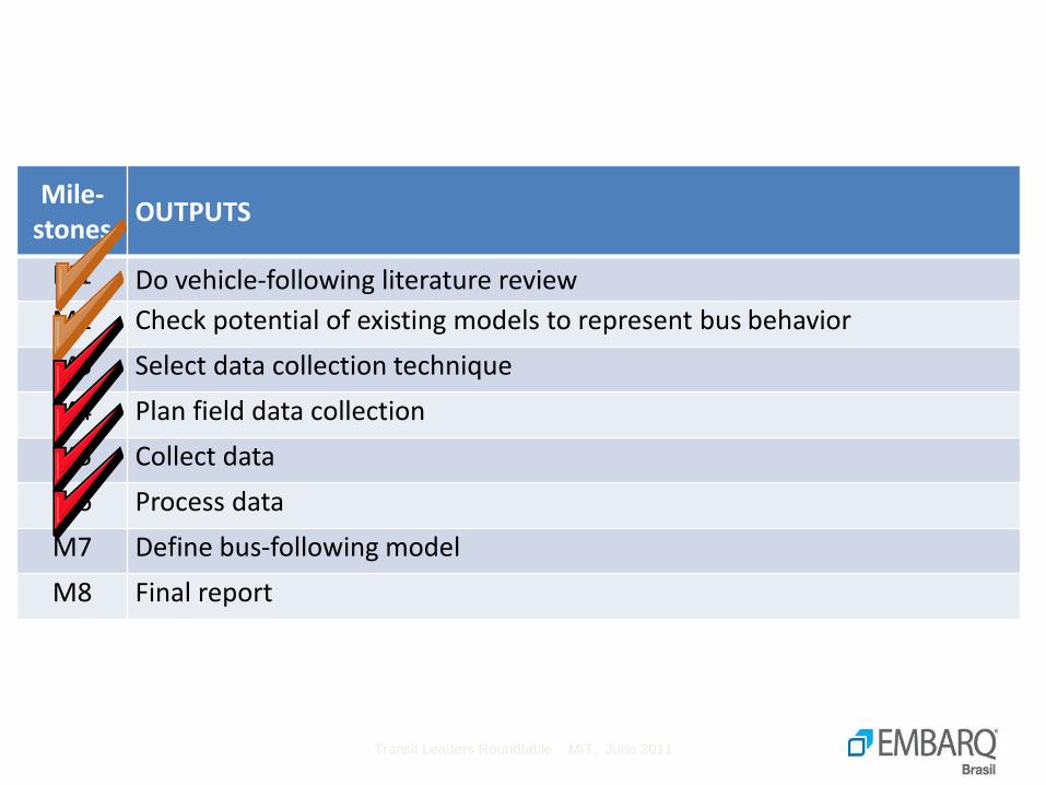
Mile-stones

OUTPUTS

M1 Do vehicle-following literature review

M2 Check potential of existing models to represent bus behavior

M3 Select data collection technique

M4 Plan field data collection

M5 Collect data

M6 Process data

M7 Define bus-following model

M8 Final report

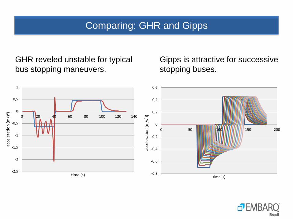
Comparing: GHR and Gipps

GHR reveled unstable for typical

bus stopping maneuvers.

-2,5

-2

-1,5

-1

-0,5

0

0,5

1

0 20 40 60 80 100 120 140

acce

lera

tio

n (

m/s

²)

time (s) -0,8

-0,6

-0,4

-0,2

0

0,2

0,4

0,6

0 50 100 150 200

acce

lera

tio

n (

m/s

²))

time (s)

Gipps is attractive for successive

stopping buses.

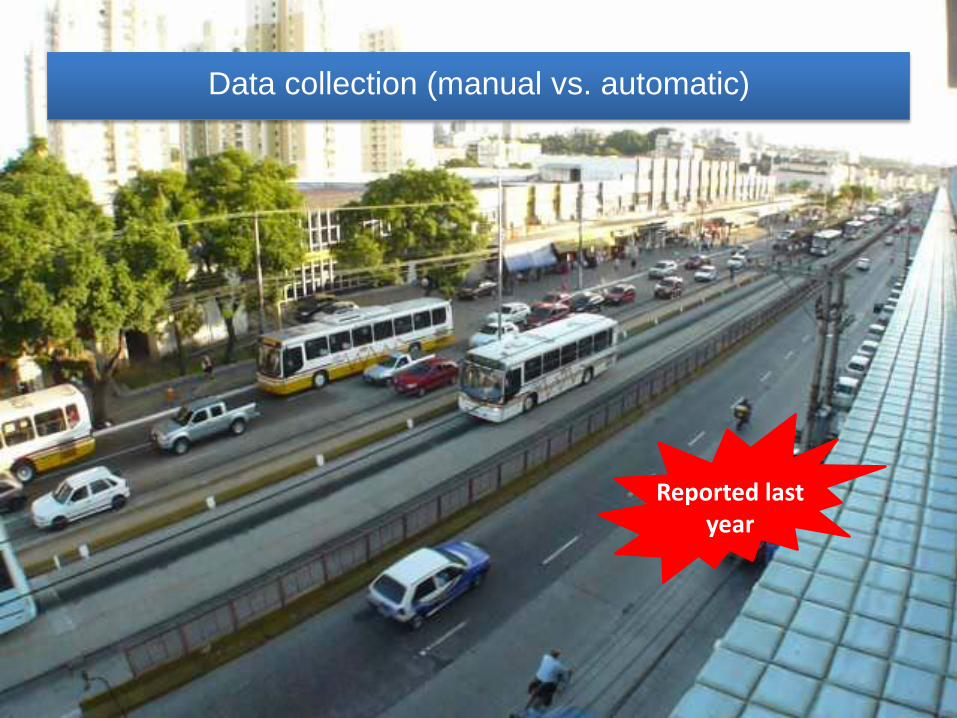
Data collection (manual vs. automatic)

Reported last year

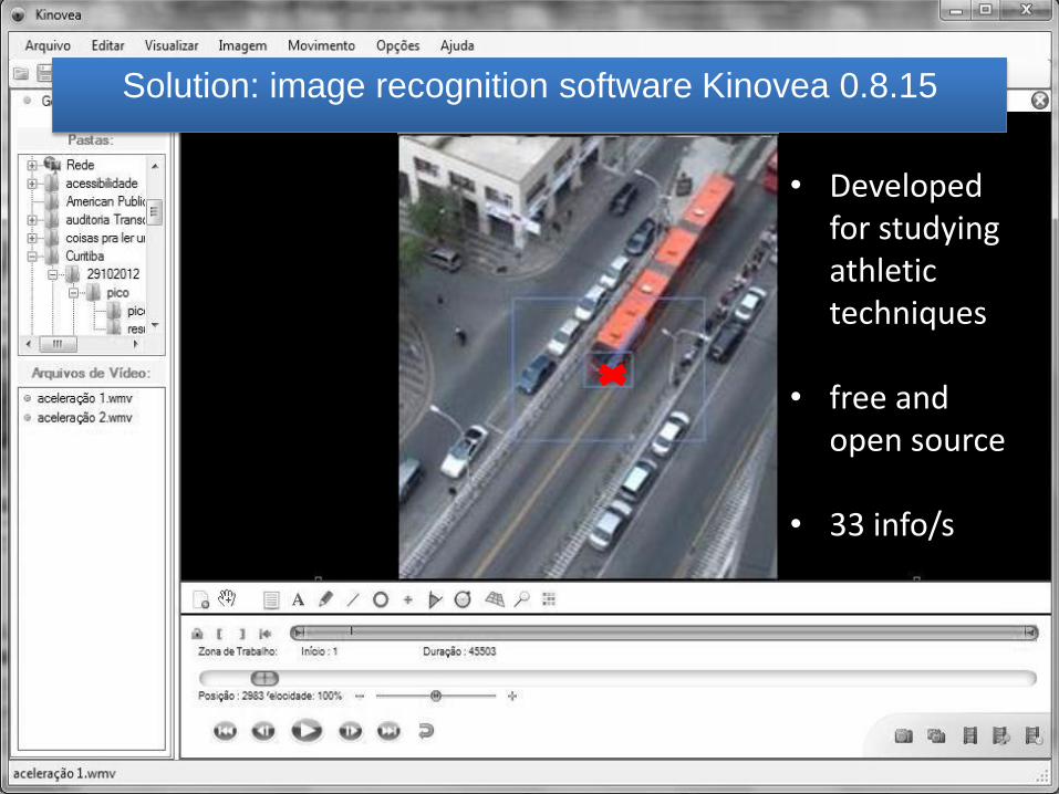
Solution: image recognition software Kinovea 0.8.15

• Developed for studying athletic techniques

• free and open source

• 33 info/s

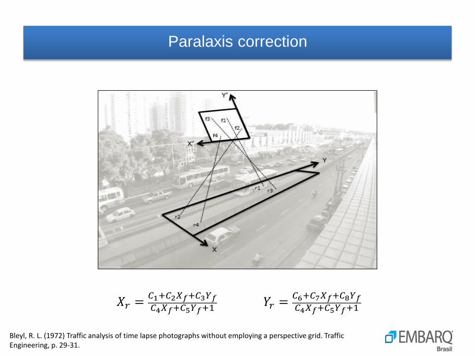
Paralaxis correction

𝑋𝑟 =𝐶1+𝐶2𝑋𝑓+𝐶3𝑌𝑓𝐶4𝑋𝑓+𝐶5𝑌𝑓+1

𝑌𝑟 =𝐶6+𝐶7𝑋𝑓+𝐶8𝑌𝑓𝐶4𝑋𝑓+𝐶5𝑌𝑓+1

Bleyl, R. L. (1972) Traffic analysis of time lapse photographs without employing a perspective grid. Traffic Engineering, p. 29-31.

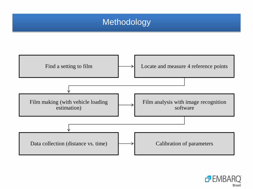
Methodology

Find a setting to film Locate and measure 4 reference points

Film making (with vehicle loading estimation)

Film analysis with image recognition software

Data collection (distance vs. time) Calibration of parameters

Calibrated models

𝑣𝑛 𝑡 + 𝑇 = 𝑏𝑛 × 𝑇 + 𝑏𝑛2 × 𝑇2 − 𝑏𝑛 × 2 × 𝑥𝑡𝑎𝑟𝑔𝑒𝑡 − 𝑥𝑛(𝑡) − 𝑣𝑛(𝑡) × 𝑇

FREE FLOW

BUS STOPPING

Static target: next station

𝑎 𝑡 + 𝑑𝑡 = 𝐴𝑚𝑎𝑥 × 1 −𝑣(𝑡)

𝑉𝑑𝑒𝑠

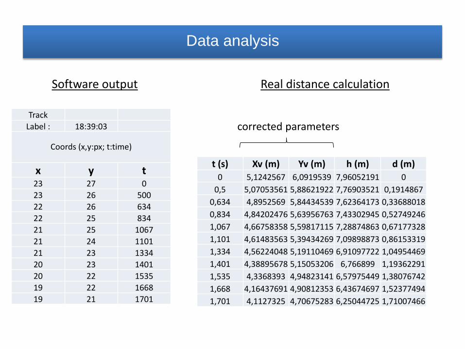
Data analysis

Track

Label : 18:39:03

Coords (x,y:px; t:time)

x y t 23 27 0

23 26 500

22 26 634

22 25 834

21 25 1067

21 24 1101

21 23 1334

20 23 1401

20 22 1535

19 22 1668

19 21 1701

Software output

t (s) Xv (m) Yv (m) h (m) d (m) 0 5,1242567 6,0919539 7,96052191 0

0,5 5,07053561 5,88621922 7,76903521 0,1914867

0,634 4,8952569 5,84434539 7,62364173 0,33688018

0,834 4,84202476 5,63956763 7,43302945 0,52749246

1,067 4,66758358 5,59817115 7,28874863 0,67177328

1,101 4,61483563 5,39434269 7,09898873 0,86153319

1,334 4,56224048 5,19110469 6,91097722 1,04954469

1,401 4,38895678 5,15053206 6,766899 1,19362291

1,535 4,3368393 4,94823141 6,57975449 1,38076742

1,668 4,16437691 4,90812353 6,43674697 1,52377494

1,701 4,1127325 4,70675283 6,25044725 1,71007466

Real distance calculation

corrected parameters

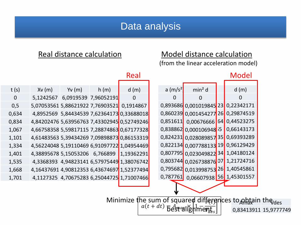
Data analysis

Model distance calculation

t (s) Xv (m) Yv (m) h (m) d (m)

0 5,1242567 6,0919539 7,96052191 0

0,5 5,07053561 5,88621922 7,76903521 0,1914867

0,634 4,8952569 5,84434539 7,62364173 0,33688018

0,834 4,84202476 5,63956763 7,43302945 0,52749246

1,067 4,66758358 5,59817115 7,28874863 0,67177328

1,101 4,61483563 5,39434269 7,09898873 0,86153319

1,334 4,56224048 5,19110469 6,91097722 1,04954469

1,401 4,38895678 5,15053206 6,766899 1,19362291

1,535 4,3368393 4,94823141 6,57975449 1,38076742

1,668 4,16437691 4,90812353 6,43674697 1,52377494

1,701 4,1127325 4,70675283 6,25044725 1,71007466

a (m/s²) v (m/s) d (m)

0 0 0

0,89368685 0,446843423 0,22342171

0,86023957 0,562115526 0,29874519

0,85161119 0,732437764 0,44523275

0,83886217 0,92789265 0,66143173

0,82423192 0,955916535 0,69393289

0,82213426 1,147473819 0,96129429

0,80779575 1,201596134 1,04180124

0,80374457 1,309297907 1,21724716

0,79568284 1,415123726 1,40545861

0,78776154 1,441119856 1,45301557

𝑎 𝑡 + 𝑑𝑡 = 𝐴𝑚𝑎𝑥 × 1 −𝑣(𝑡)

𝑉𝑑𝑒𝑠

Amax Vdes

0,83413911 15,9777749

Real distance calculation (from the linear acceleration model)

d (m)

0

0,22342171

0,29874519

0,44523275

0,66143173

0,69393289

0,96129429

1,04180124

1,21724716

1,40545861

1,45301557

d (m)

0

0,1914867

0,33688018

0,52749246

0,67177328

0,86153319

1,04954469

1,19362291

1,38076742

1,52377494

1,71007466

Real Model

min² d

0

0,001019845

0,001454277

0,00676666

0,000106948

0,028089857

0,007788133

0,023049822

0,026738876

0,013998753

0,06607938

Minimize the sum of squared differences to obtain the best alignment

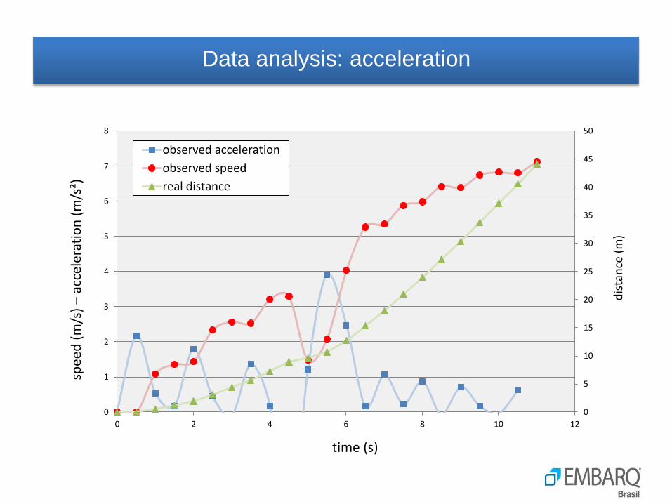
Data analysis: acceleration

0

5

10

15

20

25

30

35

40

45

50

0

1

2

3

4

5

6

7

8

0 2 4 6 8 10 12

dis

tan

ce (

m)

spee

d (

m/s

) –

acce

lera

tio

n (

m/s

²)

time (s)

observed acceleration

observed speed

real distance

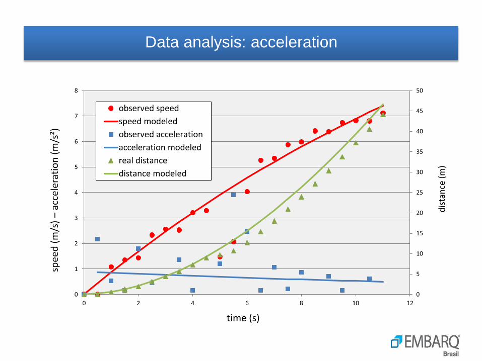
Data analysis: acceleration

0

5

10

15

20

25

30

35

40

45

50

0

1

2

3

4

5

6

7

8

0 2 4 6 8 10 12

dis

tan

ce (

m)

spee

d (

m/s

) –

acce

lera

tio

n (

m/s

²)

time (s)

observed speed

speed modeled

observed acceleration

acceleration modeled

real distance

distance modeled

Acceleration by occupancy level

0,00

0,20

0,40

0,60

0,80

1,00

1,20

1,40

1,60

0 1 2 3 4 5 6

acce

lera

tio

n (

m/s

²)

bus load levels

level 1

level 2

level 3

level 4

level 5

average

Level 1 Level 2 Level 3 Level 4 Level 5

Acceleration (m/s²)

1,07 (0,11)

0,94 (0,16)

0,92 (0,09)

0,81 (0,17)

0,80 (0,14)

Time to reach 60km/h (s)

33 (7,49)

35 (7,00)

34 (3,60)

40 (7,74)

49 (16,74)

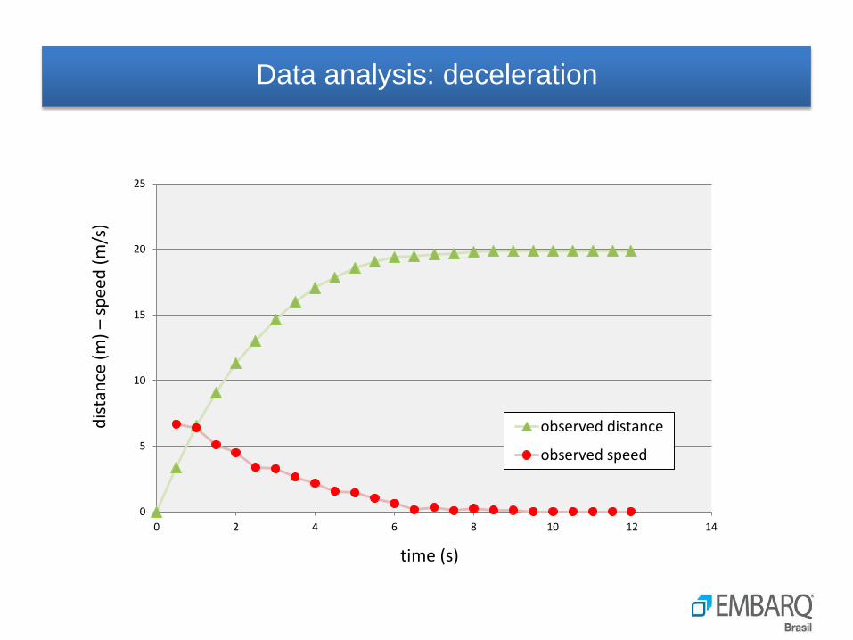
Data analysis: deceleration

0

5

10

15

20

25

0 2 4 6 8 10 12 14

dis

tan

ce (

m) –

spee

d (

m/s

)

time (s)

observed distance

observed speed

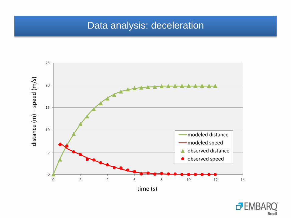
Data analysis: deceleration

0

5

10

15

20

25

0 2 4 6 8 10 12 14

dis

tan

ce (

m) –

spee

d (

m/s

)

time (s)

modeled distance

modeled speed

observed distance

observed speed

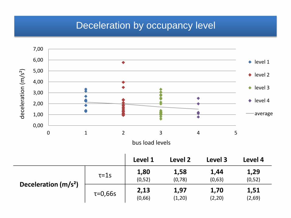
Deceleration by occupancy level

Level 1 Level 2 Level 3 Level 4

Deceleration (m/s²)

τ=1s 1,80 (0,52)

1,58 (0,78)

1,44 (0,63)

1,29 (0,52)

τ=0,66s 2,13 (0,66)

1,97 (1,20)

1,70 (2,20)

1,51 (2,69)

0,00

1,00

2,00

3,00

4,00

5,00

6,00

7,00

0 1 2 3 4 5

dec

eler

atio

n (

m/s

²)

bus load levels

level 1

level 2

level 3

level 4

average