LRFD Calibration of the Ultimate Pullout Limit Statefor Geogrid Reinforced Soil Retaining Walls

Richard J. Bathurst, Ph.D.1; Bingquan Huang, Ph.D.2; and Tony M. Allen, M.ASCE3

Abstract: The results of load and resistance factor design (LRFD) calibration are reported for the pullout limit state in geogrid reinforced soilwalls under self-weight loading and permanent uniform surcharge. Bias statistics are used to account for the prediction accuracy of theunderlying deterministic models for load and pullout capacity and the random variability in the input parameters. The paper shows thatthe current AASHTO simplified method to calculate reinforcement loads under operational conditions is overly conservative leading topoor prediction accuracy of the underlying deterministic model used in LRFD calibration. Refinements to the load and default pulloutcapacity models in the AASHTO and Federal Highway Administration guidance documents are proposed. These models generate reasonableresistance factors using a load factor of 1.35 and give a consistent probability of pullout failure of 1%. A comparison with the allowable stressdesign (ASD) past practice shows that the operational factors of safety using a reliability-based LRFD approach give factors of safety greaterthan 1.5. Regardless of the design approach (ASD or LRFD), the analysis results demonstrate that the current empirical minimum reinforce-ment length criteria will likely control the design for pullout. DOI: 10.1061/(ASCE)GM.1943-5622.0000219. © 2012 American Society ofCivil Engineers.

CE Database subject headings: Retaining structures; Geogrids; Load and resistance factor design; Calibration; Pullout; Reliability;Limit states.

Author keywords: Retaining walls; Geogrid; Load and resistance factor design; Calibration; Pullout; Reliability.

Introduction

Load and resistance factor design (LRFD) has been used in struc-tural engineering design for decades in North America. Only re-cently have AASHTO (e.g., AASHTO 2010) and the CanadianHighway Bridge Design Code (e.g., CSA 2006) recommendedLRFD for the design of all structures, including reinforced soil re-taining walls [i.e., mechanically stabilized earth walls (MSEWs)].Initial steps to migrate from allowable stress design (ASD) pastpractice (the factor of safety approach) involved simply back-calculating resistance factors for each limit state based on recom-mended factors of safety in ASD past practice (e.g., AASHTO2002) and prescribed load factors. However, this method providesno guarantee that an acceptable target probability of failure isachieved for each limit state. Furthermore, it is unlikely that theprobability of failure is the same for all limit states in a set of cal-culations (e.g., internal stability limit states for geosynthetic rein-forced soil walls) and that back-calculated limit state values are the

same for other types of retaining wall structures (e.g., metallicreinforced soil walls).

This paper reports the reliability-based LRFD calibration forthe geogrid pullout limit state in geosynthetic reinforced soil wallssubjected to soil self-weight plus permanent uniform surchargeloading. Today, calibration can be attempted because a large data-base of reinforcement loads from full-scale instrumented walls(e.g., Bathurst et al. 2008b) and geogrid pullout capacity statisticsfrom a large database of laboratory tests (Huang and Bathurst 2009)are now available.

The paper first demonstrates that the current resistance factorφ ¼ 0:90 recommended by AASHTO (2010) for reinforcementpullout for MSEW structures cannot be justified. Then, the paperproposes modifications to the current AASHTO simplified methodand a new default pullout model that can be used to improve theprediction accuracy of load and resistance capacity for the pulloutlimit state. Finally, the paper investigates the influence on the pull-out design of current empirical criteria that restrict the minimumreinforcement length regardless of pullout capacity.

LRFD Concepts

In LRFD, engineers use prescribed limit state equations andload and resistance factors specified in the design specificationsto ensure that a target probability of failure for each load carryingmember in a structure is not exceeded. The objective of LRFDcalibration in the context of the current paper is to compute loadand resistance factor values to meet this same objective usingmeasured load and resistance data rather than fitting to ASDpast practice. The fundamental limit state expression used inLRFD is

φRn ≥X

γiQni ð1Þ

1Professor and Research Director, GeoEngineering Centre at Queen’s-RMC, Dept. of Civil Engineering, Royal Military College of Canada,Kingston, ON K7K 7B4, Canada (corresponding author). E-mail:bathurst-r@rmc.ca

2Geotechnical Engineer, AMEC Environment & Infrastructure, 160Traders Blvd., Unit 110, Mississauga, ON L4Z 3K7, Canada; formerly,Ph.D. Student, GeoEngineering Centre at Queen’s-RMC, Dept. of CivilEngineering, Queen’s Univ., Kingston, ON K7L 3N6, Canada.

3State Geotechnical Engineer, State Materials Laboratory, WashingtonState Dept. of Transportation, P.O. Box 47365, Olympia, WA 98504-7365.

Note. This manuscript was submitted on August 4, 2011; approved onApril 4, 2012; published online on April 11, 2012. Discussion period openuntil January 1, 2013; separate discussions must be submitted for individualpapers. This paper is part of the International Journal of Geomechanics,Vol. 12, No. 4, August 1, 2012. ©ASCE, ISSN 1532-3641/2012/4-399–413/$25.00.

INTERNATIONAL JOURNAL OF GEOMECHANICS © ASCE / JULY/AUGUST 2012 / 399

Int.

J. G

eom

ech.

201

2.12

:399

-413

.D

ownl

oade

d fr

om a

scel

ibra

ry.o

rg b

y Q

ueen

'S U

nive

rsity

on

08/0

6/12

. For

per

sona

l use

onl

y.N

o ot

her

uses

with

out p

erm

issi

on. C

opyr

ight

(c)

201

2. A

mer

ican

Soc

iety

of

Civ

il E

ngin

eers

. All

righ

ts r

eser

ved.

where φ = resistance factor, Rn = nominal (characteristic) resis-tance, γi = load factor, and Qni = nominal (specified) load. In designspecifications, load factor values are intended to be greater than orequal to 1 and resistance factor values typically are intended to beless than or equal to 1.

It is important to emphasize that for bridge design a nominalload is not a failure load but rather a value that is a best estimateof the load under operational conditions (Harr 1987). For example,this nominal load may be a result of structure dead loads plus arepresentative vehicle load based on the statistical treatment ofbridge traffic. Conceptually, the margin of safety is largely pro-vided by the resistance side of the equation, where the resistancevalue is calculated based on the failure capacity (ultimate limitstate) or a deformation criterion (serviceability limit state) for eachelement analyzed. For the case of a steel member, the ultimate re-sistance of the member is based (typically) on the flexure or shearcapacity and the serviceability is based on a prescribed allowabledeformation.

The same concepts described previously should apply to theultimate (strength) limit states for the internal stability design ofgeosynthetic reinforced soil walls using LRFD. The reinforcementloads owing to soil self-weight can be estimated using the currentAASHTO (2010) simplified method. A common source of confu-sion and conflict with LRFD using the simplified method is thatthe underlying deterministic model used to calculate reinforcementloads is based on the active earth pressure theory or Coulombwedge analysis and, hence, the soil and critical reinforcementlayers are assumed to be simultaneously at incipient failure. Evenif this unlikely coincidence was accepted a priori at an ultimatelimit state, it is reasonable to expect that the operational loadsin the very large number of successful walls in place today are verymuch lower than the loads predicted using methods adapted fromclassical active earth pressure theory (i.e., the simplified methodand its variants) (Allen et al. 2002; Allen and Bathurst 2002b;Bathurst et al. 2008b). Furthermore, reinforcement strains in moni-tored field walls, which have behaved well under operational con-ditions, have stayed the same or even decreased with time followingconstruction (Allen and Bathurst 2002a; Miyata and Bathurst2007a, b; Tatsuoka et al. 2004; Kongkitkul et al. 2010). Hence,tensile reinforcement loads at the end-of-construction conditionare the maximum loads for LRFD design provided the original siteand boundary conditions for which the wall was designed do notchange (e.g., no unforeseen development of hydrostatic pressuresin the backfill, earthquake loading, changes in soil surcharge con-ditions, and the like).

Despite the shortcomings of limit equilibrium-based methodsfor the design of geosynthetic reinforced soil walls noted previ-ously in the context of observed behavior and LRFD calibration,the simplified method described in the AASHTO (2010) andFederal Highway Administration (FHwA) (Berg et al. 2009) guid-ance documents is the most common approach used to estimatenominal tensile loads in geosynthetic reinforcement layers in NorthAmerica using ASD or LRFD approaches.

Variations of the simplified method for steel reinforced soilwalls are also found in the AASHTO (2010), FHwA (Berg et al.2009), and BS 8006 (BSI 2010) design specifications. In general,the AASHTO simplified method for steel strip and steel grid rein-forced soil walls does well in predicting reinforcement loads underoperational conditions owing to soil self-weight (Allen et al. 2004;Bathurst et al. 2009, 2010). This is because empirical adjustmentswere made to the coefficient of earth pressure to match the mea-sured reinforcement loads in steel reinforced soil walls under op-erational conditions. Hence, a strategy to preserve the AASHTOsimplified method for the internal stability LRFD of geosynthetic

reinforced soil walls is to use an empirically adjusted model tocompute reinforcement loads under end-of-construction (opera-tional) conditions. To the best of the writers’ knowledge, no attempthas been made to adjust the AASHTO simplified method to matchthe operational tensile loads in geosynthetic reinforced soil walls.This was initially a result of the lack of measured strain (or load)data and the challenge of estimating the load in reinforcementlayers from strain measurements. These obstacles have been over-come in this study by (1) collecting data from a large number ofcarefully instrumented full-scale walls (e.g., Allen et al. 2002;Miyata and Bathurst 2007a, b); (2) developing a methodologyto estimate the reinforcement stiffness values for geosynthetic prod-ucts based on laboratory creep data (Walters et al. 2002); and (3) us-ing a suitably selected stiffness value and strain measurements toestimate the reinforcement loads in full-scale structures (e.g., Allenand Bathurst 2002a; Bathurst et al. 2005, 2008b).

LRFD Calibration Concepts

LRFD is based on reliability theory (e.g., Nowak and Collins 2000;Ang and Tang 1975, 1984; Benjamin and Cornell 1970). An over-view and history of LRFD in geotechnical engineering design hasbeen reported by Becker (1996a, b) and Kulhawy and Phoon(2002). The calibration approach in this paper follows that usedfor LRFD calibration for superstructure design in the highwaybridge design specifications in North America (Nowak 1999;Nowak and Collins 2000; Allen et al. 2005). The standard forLRFD calibration for both geotechnical and structural designadopted by the AASHTO Bridge Subcommittee (Kulicki et al.2007) refers to the Allen et al. (2005) document as the primaryreference for calibration procedures. Examples of the general ap-proach for LRFD calibration of steel grid reinforced soil walls andsteel multianchor walls have also been reported by Bathurst et al.(2008a, 2011b, c). An important feature of the general approach isthe use of bias statistics, where bias is defined as the ratio of themeasured value to the predicted (nominal) value. Bias statistics areinfluenced by model bias (i.e., the accuracy of the theoretical, semi-empirical, or empirical model used to compute the nominal load orresistance value in the limit state equation under investigation), ran-dom variation in the input parameter values, spatial variation in theinput values, the quality of the data, and the consistency in inter-pretation of the data when data are gathered from multiple sources(the typical case) (Allen et al. 2005). If the underlying deterministicmodel used to predict the load or resistance capacity is accurate andthe other sources of randomness are small, then the bias statisticshave a mean value that is close to 1 and a small coefficient of varia-tion (COV). If the underlying deterministic models give overlyconservative estimates of the reinforcement load, then adjustmentsto these models may be required to achieve sensible values for theload and resistance factors (i.e., load factor values equal to orgreater than 1 and resistance factor values equal to or less than 1).

For the case of a single load source Eq. (1) can be written as

φRn � γQQn ≥ 0 ð2Þ

where Rn = nominal computed resistance, Qn = nominal computedload, and γQ = corresponding load factor. Using bias values, Eq. (2)can be expressed as

γQXR ≥ φXQ ð3Þ

where XR = resistance bias computed as the ratio of measured re-sistance (Rm) to the calculated (predicted) nominal resistance (Rn)and XQ = load bias computed as the ratio of measured load (Qm) to

400 / INTERNATIONAL JOURNAL OF GEOMECHANICS © ASCE / JULY/AUGUST 2012

Int.

J. G

eom

ech.

201

2.12

:399

-413

.D

ownl

oade

d fr

om a

scel

ibra

ry.o

rg b

y Q

ueen

'S U

nive

rsity

on

08/0

6/12

. For

per

sona

l use

onl

y.N

o ot

her

uses

with

out p

erm

issi

on. C

opyr

ight

(c)

201

2. A

mer

ican

Soc

iety

of

Civ

il E

ngin

eers

. All

righ

ts r

eser

ved.

the calculated (predicted) nominal load (Qn). The derivation ofEq. (3) can be found in the appendices of two related papers(Bathurst et al. 2011c; Huang et al. 2012). Bathurst et al. (2008a)have pointed out that in order for Eq. (3) to be valid the bias valuesmust be uncorrelated to the calculated values (i.e., no hiddendependencies). Phoon and Kulhawy (2003) gave an example ofthe hidden dependency between the shaft capacity bias values andthe calculated capacities taken from a database of tests on laterallyloaded rigid drilled shafts.

LRFD Calibration of the Pullout Limit State

The limit state function for pullout failure of a geosyntheticreinforcement layer owing to soil self-weight plus permanent uni-form surcharge pressure is

φPc � γQTmax ≥ 0 ð4Þwhere Pc = nominal calculated pullout capacity (Rn); Tmax = nomi-nal calculated maximum reinforcement load (Qn); and γQ = corre-sponding load factor applicable to internal MSEW stability,assuming that no live load is present (called the vertical earth pres-sure load factor in AASHTO and FHwA design specifications).Eq. (3) can now represent the pullout limit state function withXR = resistance bias computed as the ratio of the measured tothe calculated (predicted) pullout capacity (Rn ¼ Pc), and XQ =load bias computed as the ratio of the measured load to the calcu-lated (predicted) nominal load (Qn ¼ Tmax).

In reliability-based design terminology the peak friction angleand cohesion term are characteristic values that are assumed tobe the best estimates of the peak soil strength input parameters(i.e., unfactored). This convention is adopted here for both loadand pullout resistance calculations when the soil shear strength val-ues are used in the computations for the nominal pullout and loadvalues. The latter are computed using the deterministic models(equations) recommended by AASHTO (2010), FHwA (Berg et al.2009), and the variants proposed by the writers. Finally, it can benoted that the general form of the limit state function expressed byEqs. (3) and (4) can be used for other internal limit states for geo-synthetic reinforced soil walls such as reinforcement rupture (oroverstressing) (Bathurst et al. 2011a, 2012).

AASHTO Simplified Method Load Model

This paper is restricted to the LRFD calibration of the ultimate(strength) limit state for geogrid pullout under soil self-weight load-ing. The maximum reinforcement load Tmax using the AASHTOsimplified method is computed as

Tmax ¼ λSvKrσv ¼ λSvKrγbðzþ SÞ ð5Þwhere λ ¼ 1; Sv = vertical spacing of the reinforcement layer; Kr =dimensionless lateral earth pressure coefficient, which is calculatedas a function of the peak soil friction angle (ϕ) and facing batter;σv = normal stress owing to the self-weight of the backfill (γb × z)and the equivalent height of the uniform surcharge pressure(S ¼ q∕γb); γb = bulk unit weight of soil; z = depth below the crestof the wall; and q = uniform distributed surcharge pressure. Theexplanation for coefficient λ is described subsequently.

Reinforcement Load Data

The reinforcement load data used in the analyses were collectedfrom full-scale laboratory test walls and field case studies reported

by Allen et al. (2002), Miyata and Bathurst (2007a, b) and Bathurstet al. (2008b). A summary of the key information is provided herefor completeness.

The database was comprised of 31 different wall sections rang-ing in height from 3 to 12.6 m. All were constructed on competentfoundations. Hence, the performance of these structures was notinfluenced by excessive settlements or failure of the foundationor wall toe. A total of 21 wall sections were constructed with avertical face; the remaining walls were constructed with facingbatter from 3 to 27°. Most walls were constructed with a hard struc-tural facing. A total of 58 data points were collected from 13 wallsections built with frictional soils (ϕ > 0, c ¼ 0) and 79 data pointsfor sections built with cohesive-frictional soils (ϕ > 0, c > 0).All shear strength values were effective stress parameters. Inmost cases, the laboratory shear strength tests were conductedon reconstituted project-specific soil samples prepared with thesame density and moisture content as measured in the actualwalls. The current AASHTO design specification allows only fric-tional (c ¼ 0) soils to be used in the reinforced soil zone. The co-hesive component of shear strength, if present, was conservativelyignored. However, to increase the database and to broaden the ap-plication of the modified load model (presented subsequently) to awider range of backfill soils, c� ϕ soil case studies were included.For these calculations the cohesive component of the soil shearstrength was included in an equivalent peak secant plane-strain fric-tion angle (ϕsec) using the conversion procedure reported by Miyataand Bathurst (2007a) and Bathurst et al. (2008b). The peak secantfriction angle was used in all load computations in this paper (un-less noted otherwise) to capture the influence of the plane-strainloading conditions that are typical for these structures in the field,to make fair comparisons between loads computed using the cur-rent model and modified load model, and to eliminate the influenceof the test method (direct shear and triaxial) on the deduced frictionangle values.

All data correspond to walls at the end of construction, and onlywalls that were judged to have performed well were considered.Good performance for walls with frictional backfills was judgedto occur if creep strains and strain rates decreased with time andthere was no evidence of failure in the reinforced soil zone, suchas cracking or slumping. Most walls had measured maximumstrains in the backfill that were less than 1% strain. Based on a re-view of available performance data for full-scale walls, Allen andBathurst (2002a) recommended that geosynthetic reinforced soilwalls should be designed to keep reinforcement strains to less than3%. Above 3% strain, contiguous shear zones may develop in thebackfill consistent with strain softening of the soil leading to aninternal failure state. Furthermore, Allen and Bathurst (2002a) con-cluded that by keeping the reinforced soil from failing, creep strainsand strain rates may be expected to decrease with time leading togood long-term wall performance.

For cohesive-frictional soils, strain hardening behavior can beexpected to lead to larger strains at peak shear capacity. Miyataand Bathurst (2007a) reviewed the performance of monitored re-inforced soil walls with c� ϕ backfills and noted that good perfor-mance was observed when postconstruction wall deformationswere less than 0.03 H or 300 mm (whichever is less) as mandatedin current Japanese design codes (e.g., see Bathurst et al. 2010).The maximum strain recorded in the database of c� ϕ soil wallsdid not exceed 3% strain when these criteria were adopted (Bathurstet al. 2008b). Hence, the empirical-based criterion that reinforce-ment strains not exceed 3% for all backfill soil types is adoptedin the current study to distinguish between reinforcement loads thatare judged to be typical of operational conditions from those thatare consistent with failure of the soil in the reinforced soil zone.

INTERNATIONAL JOURNAL OF GEOMECHANICS © ASCE / JULY/AUGUST 2012 / 401

Int.

J. G

eom

ech.

201

2.12

:399

-413

.D

ownl

oade

d fr

om a

scel

ibra

ry.o

rg b

y Q

ueen

'S U

nive

rsity

on

08/0

6/12

. For

per

sona

l use

onl

y.N

o ot

her

uses

with

out p

erm

issi

on. C

opyr

ight

(c)

201

2. A

mer

ican

Soc

iety

of

Civ

il E

ngin

eers

. All

righ

ts r

eser

ved.

Here, walls with reinforcement strains greater than 3% were notincluded in the analyses.

A total of 137 geosynthetic reinforcement load values were usedto compute load bias values. Load values were computed from themaximum strain measured in each layer of reinforcement usingthe approach described by Walters et al. (2002), who showed thatthere was good agreement between the measured loads [i.e., com-puted using in situ measured reinforcement strains and stiffness val-ues from laboratory constant load (creep) tests] and reinforcementload cell readings where these comparisons were possible.

Load Bias Statistics

Current and Modified Load Models

The constant coefficient λ was introduced in Eq. (5); λ ¼ 1 whenthe current AASHTO simplified method is used and λ ¼ 0:3 or0.15 when applied to the modified AASHTO simplified methodintroduced subsequently for frictional and cohesive-frictional back-fill soil cases, respectively. However, it is important to note that theλ values for the modified load models are determined quantitativelyby fitting to the load bias data as will be shown subsequently.The benefit of using these empirical correction factors is thatthe accuracy of the underlying deterministic model is quantitativelyimproved (on average) and this ensures reasonable LRFD calibra-tion outcomes (i.e., load factors that are greater than 1 and resis-tance factors that are less than 1) as will be demonstratedsubsequently.

Current Simplified Method (λ�1)

Fig. 1(a) shows the measured versus calculated Tmax values usingthe current AASHTO simplified method for all wall cases in thedatabase with cohesionless soil (c ¼ 0) backfills. None of the datapoints fall above the 1∶1 correspondence line. In some cases, thecalculated load values are an order of magnitude higher than themeasured value. The bias statistics are summarized in Table 1.The mean of the load bias values is μQ ¼ 0:30; hence, the measuredload values are 30% of the calculated values on average. The es-timates of the predicted Tmax are based on peak secant plane-strainfriction angles that are greater than (uncorrected) peak friction an-gles using triaxial compression or direct shear tests (Allen et al.2002). Hence, the overprediction of reinforcement loads wouldbe greater if the conversion to the peak plane-strain friction anglewas not made.

The bias data are plotted against the calculated load values inFig. 1(b). The linear regressed line reveals a visual weak trendof decreasing magnitude of bias values with increasing calculatedTmax values. As a quantitative check of this visual trend, the 95%confidence interval on the slope of the regressed line was computedand shown to be equal to �0:013 and þ0:007; these limits containzero. This confirms that at a level of significance of 5%, the nec-essary condition that bias values be independent of the calculatedloads is not violated. In the current study, the zero slope test wasapplied to similar data sets presented subsequently. In each case thezero slope test outcome was confirmed using the Spearman rankcorrelation test at a level of significance of 5%.

Fig. 1(c) shows all bias data (using lognormal values) plottedas a cumulative distribution function (CDF). A lognormal fit toall data using bias statistics (mean, μQ ¼ 0:30; coefficient ofvariation, COVQ ¼ 0:54) is judged to be a satisfactory fit to theentire data set with the possible exception of the end of the uppertail. A lognormal fit to the upper tail is also shown, which corre-sponds to the mean and COV values of 0.35 and 0.17, respectively.

Allen et al. (2005) and Bathurst et al. (2008a) have pointed outthat it is the approximation to the upper tail of the load bias datathat is important because it is the overlap between the upper tailof the load bias data and lower tail of the resistance (pullout) biasdata that strongly influences the probability of failure in reliability-based analysis.

Fig. 2 shows the normalized load data for the measured andpredicted values at the end of construction using the current sim-plified method and cohesionless soils. The maximum load Tmax in areinforcement layer is normalized with Tmxmx, which is the maxi-mum reinforcement load in the wall, and the reinforcement depth(zþ S) is normalized with the equivalent height of the wall (H þ S),

Fig. 1. Measured and predicted (calculated) reinforcement load datausing the current AASHTO simplified method for c ¼ 0 and ϕ > 0soils: (a) measured versus calculated load values; (b) load bias versuscalculated load values; (c) CDF plots for load bias data

402 / INTERNATIONAL JOURNAL OF GEOMECHANICS © ASCE / JULY/AUGUST 2012

Int.

J. G

eom

ech.

201

2.12

:399

-413

.D

ownl

oade

d fr

om a

scel

ibra

ry.o

rg b

y Q

ueen

'S U

nive

rsity

on

08/0

6/12

. For

per

sona

l use

onl

y.N

o ot

her

uses

with

out p

erm

issi

on. C

opyr

ight

(c)

201

2. A

mer

ican

Soc

iety

of

Civ

il E

ngin

eers

. All

righ

ts r

eser

ved.

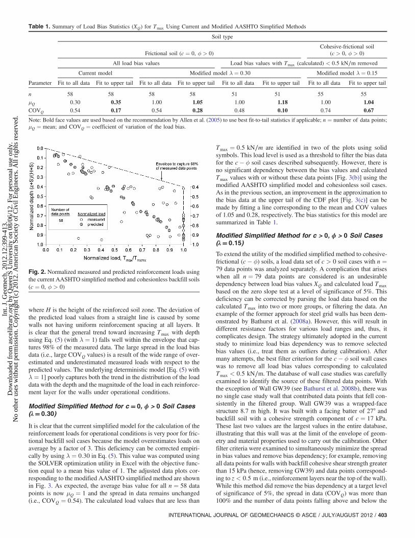
where H is the height of the reinforced soil zone. The deviation ofthe predicted load values from a straight line is caused by somewalls not having uniform reinforcement spacing at all layers. Itis clear that the general trend toward increasing Tmax with depthusing Eq. (5) (with λ ¼ 1) falls well within the envelope that cap-tures 98% of the measured data. The large spread in the load biasdata (i.e., large COVQ values) is a result of the wide range of over-estimated and underestimated measured loads with respect to thepredicted values. The underlying deterministic model [Eq. (5) withλ ¼ 1] poorly captures both the trend in the distribution of the loaddata with the depth and the magnitude of the load in each reinforce-ment layer for the walls under operational conditions.

Modified Simplified Method for c� 0, ϕ > 0 Soil Cases(λ� 0:30)

It is clear that the current simplified model for the calculation of thereinforcement loads for operational conditions is very poor for fric-tional backfill soil cases because the model overestimates loads onaverage by a factor of 3. This deficiency can be corrected empiri-cally by using λ ¼ 0:30 in Eq. (5). This value was computed usingthe SOLVER optimization utility in Excel with the objective func-tion equal to a mean bias value of 1. The adjusted data plots cor-responding to the modified AASHTO simplified method are shownin Fig. 3. As expected, the average bias value for all n ¼ 58 datapoints is now μQ ¼ 1 and the spread in data remains unchanged(i.e., COVQ ¼ 0:54). The calculated load values that are less than

Tmax ¼ 0:5 kN∕m are identified in two of the plots using solidsymbols. This load level is used as a threshold to filter the bias datafor the c� ϕ soil cases described subsequently. However, there isno significant dependency between the bias values and calculatedTmax values with or without these data points [Fig. 3(b)] using themodified AASHTO simplified model and cohesionless soil cases.As in the previous section, an improvement in the approximation tothe bias data at the upper tail of the CDF plot [Fig. 3(c)] can bemade by fitting a line corresponding to the mean and COV valuesof 1.05 and 0.28, respectively. The bias statistics for this model aresummarized in Table 1.

Modified Simplified Method for c > 0, ϕ > 0 Soil Cases(λ� 0:15)

To extend the utility of the modified simplified method to cohesive-frictional (c� ϕ) soils, a load data set of c > 0 soil cases with n ¼79 data points was analyzed separately. A complication that ariseswhen all n ¼ 79 data points are considered is an undesirabledependency between load bias values XQ and calculated load Tmaxbased on the zero slope test at a level of significance of 5%. Thisdeficiency can be corrected by parsing the load data based on thecalculated Tmax into two or more groups, or filtering the data. Anexample of the former approach for steel grid walls has been dem-onstrated by Bathurst et al. (2008a). However, this will result indifferent resistance factors for various load ranges and, thus, itcomplicates design. The strategy ultimately adopted in the currentstudy to minimize load bias dependency was to remove selectedbias values (i.e., treat them as outliers during calibration). Aftermany attempts, the best filter criterion for the c� ϕ soil wall caseswas to remove all load bias values corresponding to calculatedTmax < 0:5 kN∕m. The database of wall case studies was carefullyexamined to identify the source of these filtered data points. Withthe exception of Wall GW39 (see Bathurst et al. 2008b), there wasno single case study wall that contributed data points that fell con-sistently in the filtered group. Wall GW39 was a wrapped-facestructure 8.7 m high. It was built with a facing batter of 27° andbackfill soil with a cohesive strength component of c ¼ 17 kPa.These last two values are the largest values in the entire database,illustrating that this wall was at the limit of the envelope of geom-etry and material properties used to carry out the calibration. Otherfilter criteria were examined to simultaneously minimize the spreadin bias values and remove bias dependency; for example, removingall data points for walls with backfill cohesive shear strength greaterthan 15 kPa (hence, removing GW39) and data points correspond-ing to z < 0:5 m (i.e., reinforcement layers near the top of the wall).While this method did remove the bias dependency at a target levelof significance of 5%, the spread in data (COVQ) was more than100% and the number of data points falling above and below the

Table 1. Summary of Load Bias Statistics (XQ) for Tmax Using Current and Modified AASHTO Simplified Methods

Parameter

Soil type

Frictional soil (c ¼ 0, ϕ > 0)Cohesive-frictional soil

(c > 0, ϕ > 0)

All load bias values Load bias values with Tmax (calculated) < 0:5 kN∕m removed

Current model Modified model λ ¼ 0:30 Modified model λ ¼ 0:15

Fit to all data Fit to upper tail Fit to all data Fit to upper tail Fit to all data Fit to upper tail Fit to all data Fit to upper tail

n 58 58 58 58 51 51 55 55

μQ 0.30 0.35 1.00 1.05 1.00 1.18 1.00 1.04COVQ 0.54 0.17 0.54 0.28 0.48 0.10 0.74 0.67

Note: Bold face values are used based on the recommendation by Allen et al. (2005) to use best fit-to-tail statistics if applicable; n ¼ number of data points;μQ ¼ mean; and COVQ ¼ coefficient of variation of the load bias.

Fig. 2. Normalized measured and predicted reinforcement loads usingthe current AASHTO simplified method and cohesionless backfill soils(c ¼ 0, ϕ > 0)

INTERNATIONAL JOURNAL OF GEOMECHANICS © ASCE / JULY/AUGUST 2012 / 403

Int.

J. G

eom

ech.

201

2.12

:399

-413

.D

ownl

oade

d fr

om a

scel

ibra

ry.o

rg b

y Q

ueen

'S U

nive

rsity

on

08/0

6/12

. For

per

sona

l use

onl

y.N

o ot

her

uses

with

out p

erm

issi

on. C

opyr

ight

(c)

201

2. A

mer

ican

Soc

iety

of

Civ

il E

ngin

eers

. All

righ

ts r

eser

ved.

1∶1 correspondence line for measured versus predicted Tmax valueswas very different. This outcome demonstrates the problem of at-tempting LRFD calibration with a model that cannot capture theeffects of the many factors that influence reinforcement loads ina wall (e.g., wall facing type, facing batter, and the combined effectof soil friction and cohesive strength components, among otherfactors).

A constant coefficient value of λ ¼ 0:15 was computed usingthe filtered data set of n ¼ 55 data points and the SOLVER utility

as before. The lower λ factor from back-calibration using onlyc > 0 soils compared with λ ¼ 0:3 for the frictional soil cases isconsistent with classical notions of earth pressure theory; i.e., thehigher the cohesive shear strength component of a backfill soilthe lower the active earth force. The measured versus calculatedloads using this model are plotted in Fig. 4(a). The data points omit-ted from the calibration are represented by the solid symbols inFigs. 4(a) and 4(b). Approximations to the entire data set (n ¼ 55)and fitting to the upper tail of the lognormal CDF plot are shown in

Fig. 3. Measured and predicted (calculated) reinforcement load datausing the modified AASHTO simplified method for cohesionless(c ¼ 0, ϕ > 0) backfill soil cases: (a) measured versus calculated loadvalues; (b) load bias versus calculated load values; (c) CDF plots forload bias data

Fig. 4. Measured and predicted (calculated) reinforcement load datausing the modified AASHTO simplified method for cohesive-frictional(c > 0, ϕ > 0) backfill soil cases: (a) measured versus calculated loadvalues; (b) load bias versus calculated load values; (c) CDF plots forload bias data

404 / INTERNATIONAL JOURNAL OF GEOMECHANICS © ASCE / JULY/AUGUST 2012

Int.

J. G

eom

ech.

201

2.12

:399

-413

.D

ownl

oade

d fr

om a

scel

ibra

ry.o

rg b

y Q

ueen

'S U

nive

rsity

on

08/0

6/12

. For

per

sona

l use

onl

y.N

o ot

her

uses

with

out p

erm

issi

on. C

opyr

ight

(c)

201

2. A

mer

ican

Soc

iety

of

Civ

il E

ngin

eers

. All

righ

ts r

eser

ved.

Fig. 4(c). The corresponding bias statistics are summarized inTable 1.

Current AASHTO/FHwA Pullout Capacity Models

According to AASHTO (2010) and FHwA (Berg et al. 2009), theultimate pullout capacity for sheet geosynthetics (geotextiles andgeogrids) is estimated using

Pc ¼ 2ðF�αÞσvLe ð6a ÞAn alternative expression that is frequently used in practice is(Huang and Bathurst 2009)

Pc ¼ 2ðΨ tanϕÞσvLe ð6b Þwhere Le = anchorage length; F� and α = dimensionless parame-ters; and Ψ ¼ tanϕsg∕ tanϕ = dimensionless efficiency factor,where ϕsg = peak geosynthetic-soil interface friction angle. Inthe FHwA document (Berg et al. 2009), the following defaultvalues are recommended: α ¼ 0:8 for geogrids and α ¼ 0:6 forgeotextiles, and F� is calculated as

F� ¼ 23tanϕ ð7Þ

In the absence of project-specific data, the AASHTO (2010) andFHwA (Berg et al. 2009) guidance documents recommend thatthe soil peak friction angle be capped at ϕ ¼ 34°.

Pullout Test Database

Huang and Bathurst (2009) collected data for 478 pullout box testsfrom multiple sources. The tests were carried out in general con-formity with ASTM D6706-01 (ASTM 2001). A total of 318 geo-grid tests were identified as having failed in pullout and these testresults are used here. The reinforcement types were typical com-mercial materials and for analysis purposes were classified as high-density polyethylene (HDPE) uniaxial geogrids, polypropylene(PP) biaxial geogrids, and woven polyester (PET) geogrids. Therewere an insufficient number of geotextile pullout tests to developstatistics for this class of products and it is for this reason thatthe current study is restricted to geogrid reinforced soil walls.The majority of tests were performed with granular soils. However,approximately 25% of tests used silty sand and 2% of tests usedsandy silt. Only the peak friction angle values were reported inthe source documents used by Huang and Bathurst (2009). Hence,

for practical purposes the database corresponds to frictional (c ¼ 0,ϕ > 0) soils.

Pullout Models and Resistance Bias Statistics

Huang and Bathurst (2009) investigated the accuracy of the currentFHwA geogrid pullout model [Eq. (6a)] using two different inter-pretations of project-specific laboratory testing (which they iden-tified as Models 1 and 2) and using the current FHwA defaultmodel parameters for F�α (Model 3) including the default peakfriction angle ϕ ¼ 34°. The default model is used when project-specific pullout data are not available. As demonstrated sub-sequently, the accuracy of this model is very poor even whenproject-specific friction angles are used in calculations [i.e., projectsoil friction angle in Eq. (7)]. To overcome this deficiency Huangand Bathurst (2009) proposed two new models: a bilinear model(Model 4) and a nonlinear model (Model 5). The bias statistics weregreatly improved, particularly for the nonlinear model. In the cur-rent study, three of the five pullout models investigated by Huangand Bathurst (2009) (Models 2, 3, and 5) are used to generate pull-out (resistance) bias statistics and to carry out LRFD calibration.It should be noted that Models 2, 3, and 5 in the current studyare used with peak friction angles reported in the source referencesrather than the more conservative interpretation using the default(capped) value of ϕ ¼ 34° (Huang and Bathurst 2009). The cappedvalue is recommended in the AASHTO (2010) and FHwA (Berget al. 2009) guidance documents for design when there is noproject-specific pullout data and project soil strength data are notavailable. The model types and the related resistance bias statisticsused in the calibrations are summarized in Table 2.

Models 1 and 4 are described in the background paper by Huangand Bathurst (2009). Model 1 corresponds to the case where a sin-gle (average) value of F�α is computed from a set of pullout tests.Model 4 uses a bilinear approximation to the efficiency factor Ψ[Eq. (6b)]. As demonstrated by Huang and Bathurst (2009), bothmodels have strong bias dependencies with normal stress and,therefore, were omitted from the current study.

Model 2 captures the stress-level dependency of the geogridpullout capacity from the pullout tests. In this approach, back-calculated values of F�α using Eq. (6a) are determined from aset of tests performed on the same soil-geogrid combination at vari-ous normal stresses. A first-order (linear) approximation is thenfitted to the data. Fig. 5(a) shows that the measured (Pm) versuspredicted (Pc) resistance values plot tightly around the 1∶1 corre-spondence line. The quantitative accuracy of the model is con-firmed by the bias statistics, which have mean and COV values

Table 2. Bias Statistics for Various Pullout Capacity Model Types

Model Description Approximation to CDF plot

Bias statistics Pm∕Pc versusPc dependencyaMean μR COVR

2 First-order approximation to measured F�α Normal fit to all data 1.00 0.13 No

Lognormal fit to all data 1.00 0.13

Normal fit to lower tail (1) 1.00 0.21

Normal fit to lower tail (2) 1.17 0.27

3 FHwA method with default values

[F�α ¼ 0:8 × ð2∕3Þ tanϕ]Lognormal 1.99 0.59 Yes

5 Nonlinear model Lognormal fit to all data 1.08 0.37 No

Lognormal fit to lower tail 1.12 0.50

Note: Model 2 requires project-specific test data; Models 3 and 5 require input parameters: σv ¼ normal stress, Le ¼ anchorage length, andϕ ¼ peak friction angle of the soil. For a description of the pullout models, see Huang and Bathurst (2009).aBased on the zero-slope test and Spearman rank correlation test at a level of significance of 5%.

INTERNATIONAL JOURNAL OF GEOMECHANICS © ASCE / JULY/AUGUST 2012 / 405

Int.

J. G

eom

ech.

201

2.12

:399

-413

.D

ownl

oade

d fr

om a

scel

ibra

ry.o

rg b

y Q

ueen

'S U

nive

rsity

on

08/0

6/12

. For

per

sona

l use

onl

y.N

o ot

her

uses

with

out p

erm

issi

on. C

opyr

ight

(c)

201

2. A

mer

ican

Soc

iety

of

Civ

il E

ngin

eers

. All

righ

ts r

eser

ved.

of 1.00 and 0.13, respectively. A zero-slope test on the resistancebias values versus the predicted (calculated) capacity showedno hidden dependency at a level of significance of 5%, and forbrevity these data are not presented. Fig. 5(b) shows the CDF plotand the normal and lognormal approximations to the bias data. Forthe resistance data in the LRFD calibration, it is the lower tail of thedistribution that makes the major contribution to the computedprobability of the failure value. Neither the normal nor lognormalapproximation to the entire data set is a good fit to the lower tail.Two examples of the best fit to the lower tail based on visual fittingare plotted in Fig. 5(b). The choice for LRFD calibrations is sub-jective. In this paper, the best (normal) fit to the lower tail (2) dis-tribution was used in the calibrations because this distributioncaptured a larger portion of the lower tail. It can be noted thatthe CDF plot of the physical data has a distinctive sigmoidal shape.This shape also appeared when each of the three sets of pullout datawere plotted separately. There was no obvious reason based on areview of the original data sources to exclude data over any range ofthe CDF plot in Fig. 5(b). Interestingly, the results of a companionstudy on installation damage revealed a similar sigmoidal shape inthe CDF plots of the installation damage bias values for woven PETgeogrids (Bathurst et al. 2011a).

Model 3 corresponds to the current FHwA (Berg et al. 2009)geogrid pullout model [Eq. (6a)]. However, unlike in Model 2, thesoil-geogrid pullout tests were not carried out. Rather, the default

value α ¼ 0:8 was used and F� was computed using ϕ of the soil[Eq. (7)]. The value of ϕ used in this study was the value reportedin the source documents. Fig. 6(a) shows the measured versuspredicted pullout resistance values. Most (about 90%) of the datafall above the 1∶1 correspondence line and the bias mean isμR ¼ 1:99. Hence, Model 3 underestimates the pullout capacity bya factor of about 2 on average. This result is not unexpected whenit is recalled that in conventional ASD (factor of safety) past prac-tice the tendency has been to underestimate the resistance capacityto ensure conservative (i.e., safe) design outcomes. However,

Fig. 5. Measured and predicted resistance data using the currentAASHTO/FHwA geogrid pullout model for project-specific testing(Model 2): (a) measured versus calculated pullout resistance values;(b) CDF plots for resistance bias data

Fig. 6.Measured and predicted resistance data using the current defaultAASHTO/FHwA geogrid pullout model (Model 3): (a) measured ver-sus calculated pullout resistance values; (b) resistance bias versus cal-culated resistance values; (c) CDF plots for resistance bias data

406 / INTERNATIONAL JOURNAL OF GEOMECHANICS © ASCE / JULY/AUGUST 2012

Int.

J. G

eom

ech.

201

2.12

:399

-413

.D

ownl

oade

d fr

om a

scel

ibra

ry.o

rg b

y Q

ueen

'S U

nive

rsity

on

08/0

6/12

. For

per

sona

l use

onl

y.N

o ot

her

uses

with

out p

erm

issi

on. C

opyr

ight

(c)

201

2. A

mer

ican

Soc

iety

of

Civ

il E

ngin

eers

. All

righ

ts r

eser

ved.

excessively conservative design models can lead to unacceptableoutcomes when accepted a priori in LRFD calibration as demon-strated subsequently. In addition to excessive conservatism, there isa strong hidden dependency with the calculated resistance capacity,which is visually apparent in Fig. 6(b). The nonlinear trend independency is reasonably well represented by a power function fit-ted to the data and which is analytically related to the function plot-ted in Fig. 6(a) (see Huang and Bathurst 2009). The fitted powerfunction in Fig. 6(a) is used subsequently to improve the predictionaccuracy of the FHwA geogrid pullout model (Model 5).

Model 5 is a pullout model that accounts for the nonlinear in-fluences that cannot be captured in the original FHwA model ap-proach [Eq. (6a)] and simultaneously removes hidden dependency.The power function fitted to the data in Fig. 6(a) is used to adjustthe current AASHTO/FHwA default pullout model (Model 3). Thegeneral form of the nonlinear pullout model proposed by Huangand Bathurst (2009) is

Pcorr ¼ χðPcÞ1þκ ¼ χð2σvLeF�αÞ1þκ ð8Þ

where dimension-dependent terms χ and 1þ κ ¼ 5:70 and 0.586,respectively, when the pullout capacity is computed in units ofkN∕m. Implementation of Model 5 is a two-step process. First,the pullout capacity (Pc) is calculated using Eq. (6a) with the de-fault value for F� [Eq. (7)] and α ¼ 0:8; then, the corrected value(Pcorr) is computed using the power function expression in Eq. (8).Fig. 7(a) illustrates the prediction accuracy of Model 5. All mea-sured versus predicted pullout load data fall close to the 1∶1 cor-respondence line with a bias mean of 1.08 and COV ¼ 0:37. Thezero-slope test applied to the data plotted in Fig. 7(b) confirms thatthe dependency between the resistance bias values and the calcu-lated resistance values is negligible. These are all marked improve-ments over Model 3, which is used in the current AASHTO (2010)and FHwA (Berg et al. 2009) design specifications. Fig. 7(c) showsthat a lognormal fit to the lower tail of the resistance bias data CDFplot is visually better able to capture the distribution at low biasvalues. The pullout (resistance) bias statistics for fits to all dataand fits to the lower tail of the CDF plots corresponding to the threedifferent pullout models are summarized in Table 2.

Selection of Target Probability of Failure Pf

The objective of LRFD calibration is to select values of the resis-tance factor and load factor such that a target probability of failureis achieved for the limit state function. In this paper the target prob-ability of failure is taken as 1 in 100 (Pf ¼ 0:01), which corre-sponds to a reliability index value β ¼ 2:33. This target Pf valuehas been recommended for reinforced soil wall structures becausethey are redundant load capacity systems (Allen et al. 2005). Ifone layer fails in pullout, load is shed to the neighboring reinforce-ment layers. Pile groups are another example of a redundant loadcapacity system; failure of one pile does not lead to failure of thegroup because of load shedding to the remaining piles. Pile groupsare designed to a target reliability index value of β ¼ 2:0–2:5(Paikowsky 2004; Allen 2005), which contains β ¼ 2:33.

Selection of Load Factor γQ

There are an infinite number of load and resistance factors that cansatisfy a target Pf value. However, as noted previously it is desir-able that resistance factors are equal to or less than 1 and load fac-tors are equal to or greater than 1. The choice of load factor will beinfluenced by the current design specifications, type of structure,

and backfitting to ASD past practice (the factor of safety approach).For example, a load factor of 1.35 is currently recommended byAASHTO (2010) for reinforcement loads in reinforced soil wallsowing to soil self-weight and permanent uniform surcharge pres-sures. During the development of the AASHTO and Canadianbridge design specifications, trial load factors were initially se-lected to ensure that factored dead loads would not be exceededby actual (measured) loads in more than 3% of cases (Nowak1999; Nowak and Collins 2000). Ideally, a consistent maximumlevel of load exceedance is desirable for a set of related limit statesin bridge and bridge foundation design; however, this is not a nec-essary condition. Fig. 1(a) shows that using the current AASHTO

Fig. 7. Nonlinear geogrid pullout model (Model 5): (a) measured ver-sus calculated pullout resistance values; (b) bias values versus calcu-lated pullout resistance values; (c) CDF plots for resistance bias data

INTERNATIONAL JOURNAL OF GEOMECHANICS © ASCE / JULY/AUGUST 2012 / 407

Int.

J. G

eom

ech.

201

2.12

:399

-413

.D

ownl

oade

d fr

om a

scel

ibra

ry.o

rg b

y Q

ueen

'S U

nive

rsity

on

08/0

6/12

. For

per

sona

l use

onl

y.N

o ot

her

uses

with

out p

erm

issi

on. C

opyr

ight

(c)

201

2. A

mer

ican

Soc

iety

of

Civ

il E

ngin

eers

. All

righ

ts r

eser

ved.

simplified method and frictional soil cases, all measured values areless than the predicted values. Hence, a load factor of γQ ¼ 1:00 issatisfactory based on past LRFD calibration of bridge superstruc-ture elements. In fact, to achieve the 3% exceedance level a loadfactor of 0.65 is required for walls with frictional backfill. Thisunacceptable outcome reveals one of a number of unfortunate con-sequences of rigorous LRFD calibration for a limit state functionthat contains an excessively conservative load model.

Fig. 8 shows cumulative distribution plots for the ratio ofmeasured load to factored and unfactored reinforcement loads us-ing the modified AASHTO simplified method for frictional andcohesive-frictional soil data sets (i.e., the same data as plotted inFigs. 3 and 4). For unfactored (γQ ¼ 1:00) load data the load ex-ceedance levels are 44 and 43% for frictional and cohesive-frictional soil cases, respectively. For frictional backfill case studiesonly, a trial load factor γQ ¼ 2:00 corresponds to an exceedancelevel of about 5%. A trial load factor of γQ ¼ 2:50 gives an exceed-ance level of 5% for the cohesive-frictional soil cases. Bathurst et al.(2008a, 2011b) carried out similar analyses of measured and cal-culated design loads in steel grid reinforced soil walls using thecurrent load model in the AASHTO (2010) design specifications.They showed that a load factor of 1.75 corresponds to an exceed-ance value of about 3–4% for these structures, and a load factor of1.35 gives an exceedance value of 16%. Figs. 8(a) and 8(b) show

that the exceedance level for the geosynthetic reinforced soil wallsin our database is approximately 25% using load factor γQ ¼ 1:35specified in AASHTO (2010). To calculate the resistance factor forthe pullout limit state a load factor and target probability must beassumed a priori. In this study the results of the calculations using arange of load factors are presented.

Calibration Results

Monte Carlo simulation was used to compute the resistance factorrequired to meet a target probability of 1% for a prescribed loadfactor and using the bias statistics reported in Tables 1 and 2.The simulations were carried out using an Excel spreadsheet as de-scribed by Allen et al. (2005) and Bathurst et al. (2008a). Table 3presents the results of the calibration. The calculations were carriedout using various sets of bias statistics for various load and resis-tance model combinations. The load side included the current andmodified AASHTO methods applied to the frictional backfill soil(c ¼ 0, ϕ > 0) cases only and the modified AASHTO method forthe cohesive-frictional soil (c > 0, ϕ > 0) cases. The pullout resis-tance models were restricted to Models 2, 3, and 5. Model 3 is thecurrent AASHTO/FHwA pullout model with default values and ϕtaken as the peak friction angle in the pullout test reports used togenerate the pullout capacity statistics. Note that the resistance(pullout) bias statistics are available for cohesionless soil casesonly. Hence, calibration for the c� ϕ soil cases has been carriedout with the implicit assumption that resistance bias statistics forcohesive-frictional soils are the same as those computed for fric-tional soils.

For a given limit state and set of statistics for the random var-iables involved, there are many combinations of load and resistancevalues that can satisfy a target probability of failure. The data inTable 3 show that the computed resistance factor value (φ) in-creases linearly with the increasing value of the load factor (γQ)selected for each model/bias statistics combination. The calibrationusing the current AASHTO simplified method for the load andc ¼ 0 soils only and fit to all data (Column 1) and fit to upper tail(Column 2) together with Models 2 and 3 for the resistance sidegives φ > 1 for all γQ ≥ 1. These φ values are greater than0.90, which is the current recommended resistance factor in theAASHTO (2010) design guide for geosynthetic MSEW structuresunder self-weight loading plus permanent uniform surcharge. Moreimportantly, this outcome violates the North American limit statesdesign convention that resistance factors should be less than 1regardless of the choice of the load factor.

If the current AASHTO simplified method for load is used(Column 1) together with a load factor of γQ ¼ 1:35, then pulloutModel 5 with fit-to-tail statistics is the best choice for LRFD design(e.g., φ ¼ 1:02≈ 1). If the modified AASHTO simplified methodis used [i.e., Eq. (5) with λ ¼ 0:3], then all back-calculated resis-tance factor values computed for the case γQ ¼ 1:35 are less than 1(Columns 3 and 4) and, thus, they are consistent with the NorthAmerican LRFD convention. The resistance factors for the modi-fied AASHTO simplified method and cohesive-frictional soils[i.e., Eq. (5) with λ ¼ 0:15] and excluding the bias values forTmax < 0:5 kN∕m) are lower than for the frictional soil cases; how-ever, they are also consistently less than 1 for γQ ¼ 1:35.

Table 4 summarizes the recommended resistance factor valuesmatching the load factor of 1.35 recommended in AASHTO (2010)for MSEW structures and using the current and modified AASHTOsimplified method. The resistance factors are given for variouscombinations of load and resistance models. It should be recalledthat no restriction on the load exceedance level has been applied to

Fig. 8. Cumulative distribution plots for the ratio of measured tofactored and unfactored calculated load values using the modifiedAASHTO simplified method: (a) frictional backfill soil cases (c ¼ 0,ϕ > 0); (b) cohesive-frictional backfill soil cases (c > 0, ϕ > 0)

408 / INTERNATIONAL JOURNAL OF GEOMECHANICS © ASCE / JULY/AUGUST 2012

Int.

J. G

eom

ech.

201

2.12

:399

-413

.D

ownl

oade

d fr

om a

scel

ibra

ry.o

rg b

y Q

ueen

'S U

nive

rsity

on

08/0

6/12

. For

per

sona

l use

onl

y.N

o ot

her

uses

with

out p

erm

issi

on. C

opyr

ight

(c)

201

2. A

mer

ican

Soc

iety

of

Civ

il E

ngin

eers

. All

righ

ts r

eser

ved.

estimate the load factor for LRFD in this paper. Rather, the currentAASHTO load factor value has been accepted a priori. If the ex-ceedance of measured to factored loads is kept to 3–5%, consistentwith values assumed for LRFD design of bridge superstructure

elements (Nowak 1999), then a load factor between 2.0 and 2.5is appropriate (Fig. 8). Computations of the type reported here us-ing these larger load factors result in larger resistance factor valuesas demonstrated in Table 3.

An important benefit of using project-specific pullout testingis that the pullout capacity can be computed using Model 2.Model 2 is more accurate than the nonlinear default Model 5.The practical consequence is that the resistance factor is higher,resulting in less reinforcement anchorage length based on this limitstate calculation.

Comparison of ASD and LRFD for Pullout Using theComputed Operational Factor of Safety

It is useful to compare the actual or operational factors of safety(OFS) using various load and/or resistance calculation modelsand to compare these outcomes with ASD past practice (Bathurstet al. 2011b). For the case of a single load term (self-weight pluspermanent uniform surcharge) the predicted (design) factor ofsafety (FS) can be estimated as

FS ¼ Rn

Qn¼ γQ

φð9Þ

Table 3. Computed Resistance Factor φ for Pf ¼ 0:01 (β ¼ 2:33) and Selected Load Factors γQ

Resistance (pullout) model

LoadfactorγQ

Resistance factor φ

Current AASHTOload model c ¼ 0

Modified AASHTO load model

c ¼ 0 c > 0

(Fit to all data)(0.30, 0.54)

(Fit to tail)(0.35, 0.17)

(Fit to all data)(1.00, 0.54)

(Fit to tail)(1.05, 0.28)

(Fit to all data)(1.00, 0.74)

(Fit to tail)(1.04, 0.67)

Column 1 Column 2 Column 3 Column 4 Column 5 Column 6

Model 2 Fit to all data

(1.00, 0.13)

1.00 1.11 1.75 0.33 0.48 0.26 0.27

1.35 1.50 2.36 0.45 0.65 0.35 0.361.75 1.95 3.06 0.58 0.85 0.45 0.47

2.00 2.23 3.50 0.67 0.97 0.51 0.54

2.50 2.78 4.38 0.83 1.21 0.64 0.67

Fit to tail (2)

(1.17, 0.27)

1.00 1.01 1.04 0.30 0.37 0.24 0.25

1.35 1.36 1.41 0.40 0.50 0.33 0.341.75 1.78 1.83 0.53 0.65 0.42 0.44

2.00 2.01 2.08 0.60 0.74 0.48 0.50

2.50 2.52 2.60 0.74 0.95 0.61 0.63

Model 5 Fit to all data

(1.08, 0.37)

1.00 0.91 1.17 0.27 0.35 0.22 0.23

1.35 1.22 1.58 0.37 0.47 0.30 0.311.75 1.58 2.04 0.48 0.61 0.38 0.40

2.00 1.81 2.33 0.54 0.70 0.44 0.45

2.50 2.26 2.92 0.68 0.87 0.55 0.57

Fit to tail

(1.12, 0.50)

1.00 0.76 0.90 0.23 0.28 0.19 0.19

1.35 1.02 1.22 0.31 0.37 0.25 0.261.75 1.32 1.58 0.40 0.49 0.33 0.34

2.00 1.51 1.80 0.45 0.55 0.38 0.38

2.50 1.89 2.26 0.57 0.69 0.47 0.48

Model 3 (default

AASHTO/FHwA

model)

Ignoring

dependency

(1.99, 0.59)

1.00 1.15 1.31 0.34 0.41 0.29 0.29

1.35 1.55 1.77 0.46 0.55 0.39 0.401.75 2.00 2.29 0.60 0.71 0.51 0.52

2.00 2.29 2.62 0.69 0.82 0.58 0.59

2.50 2.86 3.28 0.86 1.02 0.72 0.74

Note: Data pairs in parentheses are mean and COVof data sets used in the Monte Carlo simulation. The bold face values are computed using selected biasstatistics for load and pullout capacity and load factor γQ ¼ 1:35.

Table 4. Summary of Recommended Resistance Factor Values for β ¼2:33 and γQ ¼ 1:35 Using the Current and Modified AASHTOSimplified Methods for Load Calculations and Various Pullout Modelsfor Resistance Capacity

Resistance (pullout)model

Resistance factor φ

Current AASHTOload model

Modified AASHTO loadmodel

λ ¼ 1, c ¼ 0λ ¼ 0:30,c ¼ 0

λ ¼ 0:15,c > 0

Model 2 1.00b 0.50 0.34

Model 5 1.00b 0.37 0.26

Model 3 (current

AASHTO model)a1.00b 0.55 0.40

aIgnoring dependency.bCalculated resistance factor values (Table 3) are greater than 1; however,the resistance factors for the design should be capped at 1.

INTERNATIONAL JOURNAL OF GEOMECHANICS © ASCE / JULY/AUGUST 2012 / 409

Int.

J. G

eom

ech.

201

2.12

:399

-413

.D

ownl

oade

d fr

om a

scel

ibra

ry.o

rg b

y Q

ueen

'S U

nive

rsity

on

08/0

6/12

. For

per

sona

l use

onl

y.N

o ot

her

uses

with

out p

erm

issi

on. C

opyr

ight

(c)

201

2. A

mer

ican

Soc

iety

of

Civ

il E

ngin

eers

. All

righ

ts r

eser

ved.

In AASHTO (2010), the recommended load and resistance factorvalues for the limit state of geogrid pullout were derived from fit-ting to FS ¼ 1:50 used in ASD past practice (Column 4 in Table 5).The OFS is defined as the ratio of the measured resistance (Rm) tothe measured load (Qm) and can be expressed as

OFS ¼ Rm

Qm¼ RnμR

QnμQ¼ FS ·

μR

μQ¼ γQ

φ·μR

μQð10Þ

The OFS [Eq. (10)] represents the true factor of safety for pulloutby correcting the underlying deterministic models for pullout andload using mean bias values μR and μQ for the entire data sets. If themodels are unbiased (i.e., μR ¼ μQ ¼ 1), OFS will be equal to FS.

The OFS values in Columns 2 and 5 in Table 5 indicate thatASD using the current AASHTO simplified method (c ¼ 0 soilsonly) for load calculations is much safer (more conservative fordesign) than the proposed LRFD approach regardless of the resis-tance model adopted in the computations. It is interesting to notethat the ASD standard practice, which is a combination of theAASHTO simplified method for load and Model 3 for resistance,corresponds to OFS ¼ 9:95, which is very much larger than thespecified (design) FS ¼ 1:5. This is not a surprise to experiencedreinforced soil wall designers who understand that pullout typicallydoes not control design and documented cases of geogrid pulloutfailure of reinforced soil walls are rare. However, this paper is thefirst attempt to quantify the actual average factor of safety using theASD approach, which despite the AASHTO mandate to standard-ize design calculations within a LRFD framework, remainscommon practice. Alternatively, the magnitude of conservativenessin ASD practice can be understood by noting that Pf ¼ 0:11% (bot-tom of Column 6), which is an order of magnitude lower than thatrecommended for LRFD design of other redundant soil-structuresystems (e.g., pile groups). The resistance factors in Column 1of Table 5 are lower using pullout Models 2 and 5 compared withthe current practice. However, recall that the estimated reinforce-ment pullout capacity values are larger using pullout Models 2and 5. The net result is that using the modified AASHTO simplifiedmethod and either of these two pullout models, the probabilities offailure will be closer to the 1% value recommended for internalstability. Alternatively stated, the potentially large conservativenessin the pullout capacity that occurs in ASD practice and significantover- or underdesign depending on the calculated pullout capacity(e.g., Fig. 6) can be reduced in principle.

Additional Design Considerations

According to the AASHTO (2010) and FHwA (Berg et al. 2009)design specifications, the length of reinforcement (L) must not be

less than 70% of the wall height and the anchorage (embedment)length (Le) must be at least 0.9 m. The first criterion was adopted tominimize geosynthetic reinforced soil wall deformations and thesecond was adopted because of uncertainty regarding the locationof the internal soil failure plane assumed in the simplified method.In some cases the length of the reinforcement may exceed 0.7 H asa result of external stability requirements. It is interesting to inves-tigate the influence of these two empirical criteria on pullout designusing the load and pullout resistance models described previously.

The ratio of the available pullout capacity (Pc) to the designpullout load (Tdes) was computed for all of the reinforcementlayers in the database used to generate load statistics. A valueof Pc∕Tdes ¼ 1 means that the pullout capacity—and, thus, theanchorage length—is controlled by the pullout model adopted forthe design; values greater than 1 mean that one of the two empiricalcriteria control the pullout design.

The available pullout capacity (Pc) based on the ASD practicewas calculated using the maximum value of Le computed usingpullout Model 3 [current default AASHTO approach; Eq. (6a)] as-suming L ¼ 0:7 H or Le ¼ 0:9 m (whichever gave the largest valueof Le). The pullout tensile design load (Tdes) was computed usingthe current AASHTO simplified method [Eq. (5) with the λ ¼ 1and c ¼ 0 soil case studies only] and FS ¼ 1:5. Hence, for theASD practice the ratio of interest is

Pc

Tdes¼ Pc

ðFS · TmaxÞð11Þ

These calculations were carried out using two different interpreta-tions of the soil peak friction angle: (1) the reported peak frictionangle based on triaxial or direct shear box testing (ϕtrx or ϕds) and(2) the converted equivalent peak plane-strain (secant) friction an-gle (ϕsec). The peak plane-strain friction angle is the same as orgreater than the triaxial or direct shear box friction angle, whichin turn is often not the same (Allen et al. 2002). Hence, using thepeak plane-strain friction angle removes the influence of this sourceof variability on the computed reinforcement loads and pulloutcapacities and, thus, ensures a fair comparison between both theASD and LRFD approaches for the frictional soil cases.

For the equivalent LRFD-based ratio and c ¼ 0 soil case studies,the maximum value of Le was computed using nonlinear pulloutModel 5 with L ¼ 0:7 H and Le ¼ 0:9 m. The pullout design loadwas computed using the proposed modified AASHTO simplifiedmethod [Eq. (5)] with λ ¼ 0:30 together with γQ ¼ 1:35 andφ ¼ 0:37. Hence, for the LRFD practice the ratio of interest is

Pc

Tdes¼ Pc�γQ

φ · Tmax

� ð12Þ

Table 5. Comparison of OFS and Probability of Failure (Pf ) Using Proposed LRFD Approach and ASD Past Practice for c ¼ 0 Backfill Soils

Resistance (pullout) model

Proposed LRFD using γQ ¼ 1:35 and modifiedAASHTO simplified method

ASD using current AASHTOsimplified method

Column 1ðφÞ

Column 2(OFS)a

Column 3[Pf ð%Þ]

Column 4(FS)b

Column 5(OFS)c

Column 6[Pf ð%Þ]d

Model 2 0.50 2.70 1 1.50 5.00 0.05

Model 5 0.37 3.94 1 1.50 5.40 0.24

Model 3 (current AASHTO model)d 0.55 4.88 1 1.50 9.95 0.11aOFS ¼ ðγQ∕φÞ · ðμR∕μQÞ and bias statistics for the entire data sets.bFS ¼ γQ∕φ ¼ 1:35∕0:9 ¼ 1:5.cOFS ¼ FS · ðμR∕μQÞ and bias statistics for the entire data sets.dIgnoring hidden dependencies.

410 / INTERNATIONAL JOURNAL OF GEOMECHANICS © ASCE / JULY/AUGUST 2012

Int.

J. G

eom

ech.

201

2.12

:399

-413

.D

ownl

oade

d fr

om a

scel

ibra

ry.o

rg b

y Q

ueen

'S U

nive

rsity

on

08/0

6/12

. For

per

sona

l use

onl

y.N

o ot

her

uses

with

out p

erm

issi

on. C

opyr

ight

(c)

201

2. A

mer

ican

Soc

iety

of

Civ

il E

ngin

eers

. All

righ

ts r

eser

ved.

The reinforcement loads and pullout capacity using the LRFD ap-proach were computed using the peak plane-strain (secant) frictionangle of the soil.

The data for all three calculation sets are plotted in Fig. 9(a).As may be expected, the lowest ratios of Pc∕Tdes for the currentASD practice correspond to the most conservative interpretationof the peak friction angle. Examination of the computed Le valuesrevealed that for the available case studies the 0.9-m embedmentlength would not control the design. The data in Fig. 9(a) showthat regardless of the choice of soil friction angle or design method,the empirical criterion L = 0.7 H controls the reinforcement embed-ment length for the design. Most of the computed ratio (Pc∕Tdes)values fall in the range of 10–100.

For cohesive-frictional soils the pullout LRFD design load wascomputed using the proposed modified AASHTO simplifiedmethod [Model 5, Eq. (5) with λ ¼ 0:15 together with γQ ¼1:35 and φ ¼ 0:26]. Note that to carry out the calculations for

the cohesive-frictional soils an equivalent peak secant plane-strainfriction angle (ϕsec) was computed using the conversion procedurereported by Miyata and Bathurst (2007a) and Bathurst et al.(2008b) and noted previously in the paper.

The computed (Pc∕Tdes) ratios are plotted against the normal-ized depth below the wall crest in Fig. 9(b). The ratio values arespread over a wider range than for the frictional soil cases; however,again the empirical criterion L ≥ 0:7 H controls the design. Finally,for both data plots there is no pronounced visual trend of increasingdesign conservatism with depth.

Conclusions

This paper reports the results of rigorous LRFD calibration for thegeogrid pullout limit state in geosynthetic reinforced soil wallsowing to soil self-weight plus permanent uniform surcharge load-ing. The general approach follows the LRFD calibration method-ology described by Allen et al. (2005) and Bathurst et al. (2008a,2011b), which is consistent with the methods used to develop theload and resistance factors for bridge superstructures (Nowak andCollins 2000).

The results of the calibration show that while the current LRFDdesign practice is safe, the current resistance factor φ ¼ 0:90 rec-ommended by AASHTO (2010) for the reinforcement pullout limitstate in mechanically stabilized earth structures under soil self-weight is problematic for the case of geosynthetic reinforced soilwalls. This is largely owing to the very conservative load estimatesusing the AASHTO simplified method, which leads to poor predic-tion accuracy of the underlying deterministic tensile load model.The combination of AASHTO-recommended load factor γQ ¼1:35 and the excessively conservative model accuracy for tensileload and default pullout capacity make it impossible to generateresistance factors less than 1, consistent with LRFD convention.The explanation for this unfortunate outcome is that before the sim-plified method was first adopted no attempt was made to empiri-cally adjust the model to match the estimates of reinforcement loadsunder operational conditions (unlike the steel reinforcement modelsrecommended by AASHTO).

To overcome these problems, modifications to the currentAASHTO simplified method are proposed and a new default pull-out model by Huang and Bathurst (2009) is used to improve theprediction accuracy of the load and resistance capacity for the pull-out limit state. These new models result in reasonable resistancefactor values (i.e., less than 1) and match a target minimum prob-ability of failure of 1% when the current AASHTO-recommendedload factor of γQ ¼ 1:35 is used. Depending on the reinforcedsoil type (frictional or cohesive-frictional) and the pullout modeladopted, the resistance factor varies in the range of φ ¼0:26� 0:50 (see the fit-to-tail values in Table 4). Although thesevalues are lower than φ ¼ 0:90 recommended by AASHTO,the load values are on average 30% of the predicted values usingthe current AASHTO simplified method, and the pullout capacitypredictions using the AASHTO default model are a factor of 2higher, on average. The predicted load and pullout capacity valuesusing the new models described in this paper are statistically moreaccurate based on the measured values (i.e., the bias mean is closerto 1 and the COVof the bias values are lower). An important prac-tical benefit of using Model 2 with actual laboratory pullout dataover the nonlinear default Model 5 is that the former approachallows a higher resistance factor to be used in design; the resultis shorter reinforcement lengths and, hence, more cost-effectivewall design outcomes.

Fig. 9. Ratio of pullout capacity to pullout design load versus normal-ized depth using the ASD and proposed LRFD approaches and invok-ing empirical restrictions on the minimum reinforcement length:(a) frictional soil wall cases; (b) cohesive-frictional soil wall cases(LRFD approach only)

INTERNATIONAL JOURNAL OF GEOMECHANICS © ASCE / JULY/AUGUST 2012 / 411

Int.

J. G

eom

ech.

201

2.12

:399

-413

.D

ownl

oade

d fr

om a

scel

ibra

ry.o

rg b

y Q

ueen

'S U

nive

rsity

on

08/0

6/12

. For

per

sona

l use

onl

y.N

o ot

her

uses

with

out p

erm

issi

on. C

opyr

ight

(c)

201

2. A

mer

ican

Soc

iety

of

Civ

il E

ngin

eers

. All

righ

ts r

eser

ved.

It is very important to emphasize that the modified load andpullout models proposed here and the corresponding resistancefactors should only be used for walls that fall within the envelopeof structures that were used to perform the LRFD calibrations in-cluding similar materials, site conditions, and soil-geogrid combi-nations. This envelope can be found in the background papers byAllen et al. (2002, 2003), Miyata and Bathurst (2007a, b), Bathurstet al. (2008b), and Huang and Bathurst (2009). The designer mustdecide if the cohesive strength component for the reinforced soil atthe end of construction is available over the life of the structure; ifnot, the cohesion term can be set to zero and the wall designedusing the frictional component of soil strength only. This will resultin safe wall designs provided the structure falls within the afore-mentioned database limits.

An attempt was made in this paper to extend the currentAASHTO simplified method for reinforcement load to cohesive-frictional soils by using the same empirical backfitting techniqueemployed to improve the accuracy of the current AASHTO sim-plified method for cohesionless soils. However, the spread in thebias statistics and, hence, the accuracy of the method can be seento be quantifiably lower. This demonstrates that the underlying(modified) deterministic model for reinforcement load predictionsunder operational conditions cannot adequately capture the quan-titative influence of wall facing type, facing batter, and combinedsoil friction and cohesive strength components (among other fac-tors) on reinforcement loads.

Finally, the paper demonstrates that regardless of which designmethod is adopted (ASD past practice with a factor of safety of 1.5or the proposed LRFD approach with newmodels for load and pull-out capacity), the length of reinforcement will likely be controlledby current empirical criteria that restrict the minimum reinforce-ment length to not less than 70% of the wall height and the anchor-age length to not less than 0.9 m. A practical outcome is that for the31 wall sections used to generate load statistics, these empiricalcriteria result in walls with probabilities of pullout failure thatare likely orders of magnitude less than 1%. This observation leadsto the recommendation that these empirical constraints should bereviewed. Provided that other serviceability criteria such as walldisplacements are not impacted, these empirical length criteriacould be relaxed and geosynthetic reinforced soil walls designedto the same target probability of failure for all internal stability limitstates.

This paper has been restricted to LRFD calibration of the pulloutlimit state for geosynthetic reinforced soil walls under soil self-weight and permanent uniform surcharge loading. A similar ap-proach can be used for other internal/facing stability limit statesincluding reinforcement tensile rupture (Bathurst et al. 2011a,2012) and reinforcement-facing connection failure.

Acknowledgments

Financial support for this study was provided by the NaturalSciences and Engineering Research Council (NSERC) of Canada,grants from the Department of National Defence (Canada), theMinistry of Transportation of Ontario, and the following U.S.State Departments of Transportation: Alaska, Arizona, California,Colorado, Idaho, Minnesota, New York, North Dakota, Oregon,Utah, Washington, and Wyoming.

Notation

The following symbols are used in this paper:c = soil cohesion;

COVQ = coefficient of variation of the load bias;COVR = coefficient of variation of the resistance bias;

F� = dimensionless pullout model parameter;H = height of wall;Kr = dimensionless lateral earth pressure coefficient;L = length of reinforced soil zone;Le = anchorage length;n = number of data points;Pc = nominal calculated pullout capacity;

Pcorr = corrected pullout capacity using the nonlinear model;Pf = probability of failure;Qm = measured load;

Qni, Qn = nominal (specified or computed) load;q = uniform distributed surcharge pressure;

Rm = measured resistance;Rn = nominal (characteristic or computed) resistance;S = equivalent height of uniform surcharge pressure

(S ¼ q∕γb);Sv = vertical spacing of the reinforcement layer;

Tdes = maximum design reinforcement load in the layer;Tmax = nominal calculated maximum reinforcement load in a

reinforcement layer;Tmxmx = maximum reinforcement load in the wall;

XR = resistance bias computed as the ratio of the measuredresistance to the calculated resistance;

XQ = load bias computed as the ratio of the measured load tocalculated load;

z = depth below the crest of the wall;α = dimensionless pullout model parameter;β = reliability index;γb = bulk unit weight of the soil;γi = load factor i;γQ = load factor for soil self-weight plus permanent uniform

surcharge pressure;κ, χ = dimensionless pullout model parameters;

λ = dimensionless load model coefficient;μQ = mean of load bias;μR = mean of resistance bias;σv = normal stress owing to the self-weight of the backfill

and uniform surcharge pressure;φ = resistance factor;ϕ = peak soil friction angle;

ϕds = peak friction angle from the direct shear box test;ϕsec = peak plane-strain secant friction angle;ϕsg = peak geosynthetic-soil interface friction angle;ϕtrx = peak friction angle from the triaxial compression test;

andΨ ¼ tanϕsg∕ tanϕ = dimensionless efficiency factor for pullout.

References

AASHTO. (2002). Standard specifications for highway bridges, 17th Ed.,AASHTO, Washington, DC.

AASHTO. (2010). LRFD bridge design specifications, 5th Ed., AASHTO,Washington, DC.

Allen, T. M. (2005). Development of geotechnical resistance factors anddowndrag load factors for LRFD foundation strength limit state design,Publication No. FHWA-NHI-05-052, Federal Highway Administration,Washington, DC.

Allen, T. M., and Bathurst, R. J. (2002a). “Observed long-term perfor-mance of geosynthetic walls, and implications for design.” Geosynth.Int., 9(5–6), 567–606.

Allen, T. M., and Bathurst, R. J. (2002b). “Soil reinforcement loads in geo-synthetic walls at working stress conditions.” Geosynth. Int., 9(5–6),525–566.

412 / INTERNATIONAL JOURNAL OF GEOMECHANICS © ASCE / JULY/AUGUST 2012

Int.

J. G

eom

ech.

201

2.12

:399

-413

.D

ownl

oade

d fr

om a

scel

ibra

ry.o

rg b

y Q

ueen

'S U

nive

rsity

on

08/0

6/12

. For

per

sona

l use

onl

y.N

o ot

her

uses

with

out p

erm

issi

on. C

opyr

ight

(c)

201

2. A

mer

ican

Soc

iety

of

Civ

il E

ngin

eers

. All

righ

ts r

eser

ved.

Allen, T. M., Bathurst, R. J., and Berg, R. R. (2002). “Global level of safetyand performance of geosynthetic walls: An historical perspective.”Geosynth. Int., 9(5–6), 395–450.

Allen, T. M., Bathurst, R. J., Holtz, R. D., Lee, W. F., and Walters, D. L.(2004). “A new working stress method for prediction of loads insteel reinforced soil walls.” J. Geotech. Geoenviron. Eng., 130(11),1109–1120.

Allen, T. M., Bathurst, R. J., Holtz, R. D., Walters, D. L., and Lee, W. F.(2003). “A new working stress method for prediction of reinforcementloads in geosynthetic walls.” Can. Geotech. J., 40(5), 976–994.

Allen, T. M., Nowak, A. S., and Bathurst, R. J. (2005). “Calibration todetermine load and resistance factors for geotechnical and structuraldesign.” Circular E-C079, Transportation Research Board, NationalResearch Council, Washington, DC.

Ang, A. H.-S., and Tang, W. H. (1975). Probability concepts in engineeringplanning and design, basic principles, Vol. 1, Wiley, New York.

Ang, A. H.-S., and Tang, W. H. (1984). Probability concepts in engineeringplanning and design, decision, risk and reliability, Vol. 2, Wiley,New York.

ASTM. (2001). Standard test method for measuring geosynthetic pulloutresistance in soil, D6706-01, West Conshohocken, PA.

Bathurst, R. J., Allen, T. M., and Nowak, A. S. (2008a). “Calibration con-cepts for load and resistance factor design (LRFD) of reinforced soilwalls.” Can. Geotech. J., 45(10), 1377–1392.

Bathurst, R. J., Allen, T. M., and Walters, D. L. (2005). “Reinforcementloads in geosynthetic walls and the case for a new working stress designmethod.” Geotext. Geomembr., 23(4), 287–322.

Bathurst, R. J., Huang, B., and Allen, T. M. (2011a). “Interpretation ofinstallation damage testing for reliability-based analysis and LRFDcalibration.” Geotext. Geomembr., 29(3), 323–334.

Bathurst, R. J., Huang, B., and Allen, T. M. (2011b). “Load and resistancefactor design (LRFD) calibration for steel grid reinforced soil walls.”Georisk: Assess. Manage. Risk Eng. Syst. Geohaz., 5(3–4), 218–228.

Bathurst, R. J., Huang, B., and Allen, T. M. (2012). “Interpretation of lab-oratory creep testing for reliability-based analysis and load and resis-tance factor design (LRFD) calibration.” Geosynth. Int., 19(1), 39–53.

Bathurst, R. J., Miyata, Y., and Allen, T. M. (2010). “Facing displacementsin geosynthetic reinforced soil walls.” Proc., Earth Retention Conf. 3(ER2010), ASCE Geo-Institute, Bellevue, WA, August 1–4, ASCE,Reston, VA, 442–459.

Bathurst, R. J., Miyata, Y., and Konami, T. (2011c). “Limit states designcalibration for internal stability of multi-anchor walls.” Soils Found.,51(6), 1051–1064.

Bathurst, R. J., Miyata, Y., Nernheim, A., and Allen, T. M. (2008b).“Refinement of K-stiffness method for geosynthetic reinforced soilwalls.” Geosynth. Int., 15(4), 269–295.

Bathurst, R. J., Nernheim, A., and Allen, T. M. (2009). “Predicted loads insteel reinforced soil walls using the AASHTO simplified method.”J. Geotech. Geoenviron. Eng., 135(2), 177–184.

Becker, D. E. (1996a). “Eighteenth Canadian Geotechnical Colloquium:Limit states design for foundations. Part I. An overview of the founda-tion design process.” Can. Geotech. J., 33(6), 956–983.

Becker, D. E. (1996b). “Eighteenth Canadian Geotechnical Colloquium:Limit states design for foundations. Part II. Development for the na-tional building code of Canada.” Can. Geotech. J., 33(6), 984–1007.

Benjamin, J. R., and Cornell, C. A. (1970). Probability, statistics, anddecision for civil engineers, McGraw-Hill, New York.

Berg, R. R., Christopher, B. R., and Samtani, N. C. (2009). “Design of me-chanically stabilized earth walls and reinforced soil slopes—volume 1.”Rep. No. FHWA-NHI-10-024, Federal Highway Administration,Washington, DC.

British Standards Institution (BSI). (2010). “Code of practice for strength-ened/reinforced soil and other fills.” BS 8006, BSI, Milton Keynes, U.K.

Canadian Standards Association (CSA). (2006). “Canadian highway bridgedesign code.” CSA Standard S6-06, CSA, Toronto.

Harr, M. E. (1987). Reliability-based design in civil engineering, McGraw-Hill, New York.

Huang, B., and Bathurst, R. J. (2009). “Evaluation of soil-geogrid pulloutmodels using a statistical approach.” Geotech. Test. J., 32(6), 489–504.

Huang, B., Bathurst, R. J., and Allen, T. M. (2012). “Load and resistancefactor design (LRFD) calibration for steel strip reinforced soilwalls.” J. Geotech. Geoenviron. Eng., 10.1061/(ASCE)GT.1943-5606.0000665 (Nov. 17, 2011).

Kongkitkul, W., Tatsuoka, F., Hirakawa, D., Sugimoto, T., Kawahata, S.,and Ito, M. (2010). “Time histories of tensile force in geogrid arrangedin two full-scale high walls.” Geosynth. Int., 17(1), 12–33.

Kulhawy, F. H., and Phoon, K.-K. (2002). “Observations on geotechnicalreliability-based design development in North America.” Foundationdesign codes and soil investigation in view of international har-monization and performance based design, Y. Honjo, O. Kusakabe,K. Matsui, M. Kouda and G. Pokharel, eds., Balkema, Lisse,Netherlands, 31–48.

Kulicki, J. M., Prucz, Z., Clancy, C. M., Mertz, D. R., and Nowak, A. S.(2007). “Updating the calibration report for AASHTO LRFD code.”Final Rep. NCHRP 20-07/186, Transportation Research Board,Washington, DC.

Miyata, Y., and Bathurst, R. J. (2007a). “Development of the K-stiffnessmethod for geosynthetic reinforced soil walls constructed with c-ϕsoils.” Can. Geotech. J., 44(12), 1391–1416.

Miyata, Y., and Bathurst, R. J. (2007b). “Evaluation of K-stiffness methodfor vertical geosynthetic reinforced granular soil walls in Japan.”Soils Found., 47(2), 319–335.

Nowak, A. S. (1999). “Calibration of LRFD bridge design code.” NCHRPRep. 368, National Cooperative Highway Research Program, Transpor-tation Research Board, Washington, DC.

Nowak, A. S., and Collins, K. R. (2000). Reliability of structures, McGraw-Hill, New York.

Paikowsky, S. G. (2004). “Load and resistance factor design (LRFD) fordeep foundations.” NCHRP Rep. 507, National Cooperative HighwayResearch Program, Transportation Research Board, Washington, DC.

Phoon, K.-K., and Kulhawy, F. H. (2003). “Evaluation of model uncertain-ties for reliability-based foundation design.” Applications of statisticsand probability in civil engineering, A. Der Kiureghian, S. Madanatand J. M. Pestana, eds., Millpress, Rotterdam, Netherlands, 1351–1356.

Tatsuoka, F., Hirakawa, D., Shinoda, M., Kongkitkul, W., and Uchimura, T.(2004). “An old but new issue: Viscous properties of polymer geosyn-thetic reinforcement and geosynthetic-reinforced soil structures.” Proc.,3rd Asian Regional Conf. on Geosynthetics (GeoAsia 2004), KeynoteLecture, J. B. Shim, C. Yoo and H.-Y. Jeon, eds., Korean GeosyntheticsSociety, Seoul, Korea, 29–77.

Walters, D. L., Allen, T. M., and Bathurst, R. J. (2002). “Conversion ofgeosynthetic strain to load using reinforcement stiffness.” Geosynth.Int., 9(5–6), 483–523.

INTERNATIONAL JOURNAL OF GEOMECHANICS © ASCE / JULY/AUGUST 2012 / 413

Int.

J. G

eom

ech.

201

2.12

:399

-413

.D

ownl

oade

d fr

om a

scel

ibra

ry.o

rg b

y Q

ueen

'S U

nive

rsity

on

08/0

6/12

. For

per

sona

l use

onl

y.N

o ot

her

uses

with

out p

erm

issi

on. C

opyr

ight

(c)

201

2. A

mer

ican

Soc

iety

of

Civ

il E

ngin

eers

. All

righ

ts r

eser

ved.