lqresnet: a deep neural network architecture for learning

LQResNet: A Deep Neural NetworkArchitecture for Learning Dynamic Processes

Pawan Goyal∗ Peter Benner†

∗Max Planck Institute for Dynamics of Complex Technical Systems, 39106 Magdeburg, Germany.Email: [email protected],

†Max Planck Institute for Dynamics of Complex Technical Systems, 39106 Magdeburg, Germany.Email: [email protected],

Mathematical modeling is an essential step, for example, to analyze the transient be-havior of a dynamical process and to perform engineering studies such as optimizationand control. With the help of first-principles and expert knowledge, a dynamic model canbe built. However, for complex dynamic processes, appearing, e.g., in biology, chemicalplants, neuroscience, financial markets, this often remains an onerous task. Hence, data-driven modeling of the dynamics process becomes an attractive choice and is supported bythe rapid advancement in sensor and measurement technology. A data-driven approach,namely operator inference framework, models a dynamic process, where a physics-informedstructure of the nonlinear term is assumed. In this work, we suggest combining the opera-tor inference with certain deep neural network approaches to infer the unknown nonlineardynamics of the system. The approach uses recent advancements in deep learning andprior knowledge of the process if possible. We briefly also discuss several extensions andadvantages of the proposed methodology. We demonstrate that the proposed methodologyaccomplishes the desired tasks for dynamics processes encountered in neural dynamics andthe glycolytic oscillator.

Keywords: Artificial intelligence, machine learning, deep learning, dynamical systems,scientific machine learning

Introduction

With the rapid development in sensor and measurement technology, time-series data of processes havebecome available in large amounts with high accuracy. Machine learning and data science play animportant role in analyzing and perceiving information of the underlying process dynamics from thesedata. Building a model describing the dynamics is vital in designing and optimizing various processes,as well as predicting their long-term transient behavior. Inferring a dynamic process model from data,often called system identification, has a rich history; see, e.g., [30,46]. While linear system identificationis well established, nonlinear system identification is still far from being as good understood as forlinear systems, despite having a similarly long research history, see, e.g., [25, 44]. Nonlinear systemidentification often relies on a good hypothesis of the model; thus, it is not entirely a black-boxtechnology. Fortunately, there are several scenarios where one can hypothesize a model structure basedon a good understanding of the underlying dynamic behavior using expert knowledge or experience.Towards nonlinear system identification, a promising approach based on a symbolic regression wasproposed [4] to determine the potential structure of a nonlinear system. The method discovers a

Preprint. 2021-03-30

arX

iv:2

103.

0224

9v2

[cs

.LG

] 2

7 M

ar 2

021

mailto:[email protected]

mailto:[email protected]

P. Goyal, P. Benner: A Deep Neural Network Architecture for Learning Dynamic Processes 2

dynamical system solely from data. However, the approach is computationally expensive; thus, itis not suitable for a large-scale dynamical system. Also, one needs to take care of the overfittingby using the Pareto front that balances model complexity and data fitting [4]. If nonlinearities areonly known to belong to a certain class of mathematical functions (a dictionary of functions), sparseregression (see, e.g., [45]) and compressive sensing (see, e.g., [7,14]) based approaches have emerged asa kind of dictionary learning methods for nonlinear models, including dynamical systems. Here, it isobserved that given a high-dimensional nonlinear function space, the process dynamics can often beaccurately described by only a few terms from the dictionary [6, 33, 35, 39, 41, 47]. Consequently, oneobtains an interpretable and parsimonious process model. However, the success of these approacheshighly depends on the quality of the constructed dictionary, i.e., the candidate nonlinear functionspace [6]. Thus, dictionaries need to be generated carefully using expert knowledge. In addition tothese, there exist other techniques to infer a model of a dynamic process, for instance from time-seriesdata [11,21], equation-free modeling [22,49], dynamical models inference [12,13,43]. In the category ofequation-free modeling, dynamical mode decomposition [38, 42, 48] has also shown promising results.Moreover, deep learning (DL) approaches have been developed successfully for this task. They havethe potential to build a model using only the time-history of dependent variables. For this, a deepneural network (DNN) is typically used, which can be understood as a composition of functions sincethe output of a layer is the input of the next layer. DNNs have shown phenomenal performance acrossvarious disciplines [19, 24, 27] (e.g., image classification, speech recognition, medical image analysis,to name a few). A primary reason for DNNs’ success is that each layer learns a particular featurerepresentation of the input, thus describing a complex function representation. Among several existingDNN architectures, Residual Neural Networks (ResNet) [20] closely resemble integration schemes (e.g.,an Euler-type integration) for ordinary differential equations (ODEs). Inspired by this, there aremethodological advances for inferring ODEs from data [9].

Furthermore, in recent years, scientific machine learning has emerged as a discipline that combinesclassical mechanistic modeling and numerical simulation with machine learning techniques. The expec-tation here is that incorporating existing scientific knowledge allows the (physical) interpretability ofmodels while requiring less training data. Here, it is important to note that engineering processes oftendo not yield the same amount of data as typical socio-economic big data applications, so overfitting isoften encountered. This can be attenuated by including physical constraints during learning, therebyreducing the network parameters or providing a better-suited network design. Operator inferenceapproaches fall into this category; see, e.g., [2, 34]. Furthermore, physics-informed neural networks(PINN) [37] also employ the existing physical knowledge to improve the learning process that, as anoutput, yields the solution of a partial differential equation. However, as of yet, PINNs assume thestructure of the physical model to be fully known, which is not available in a complex dynamic process.

In the following section, we propose a DNN architecture dedicated to learning dynamical systemsfrom data while incorporating certain structural assumptions implied by the underlying physics.

LQResNet: A deep network architecture for learning nonlineardynamics

In this work, we focus on identifying a dynamical model by using not only collected data in simulationsor experiments but also available expert knowledge and physical laws about the process. In general,we aim at inferring a nonlinear dynamical system of the form:

x(t) = g(x(t)), (1)

where the vector x(t) ∈ Rn denotes the state at time t, and the function g(·) : Rn → Rn is acontinuous differentiable function, describing the dynamics of the system. We shall later on discussits extension to dynamical systems with control and parameters, and its discrete version. In principle,we are interested in determining the function g from data. To that aim, we observe time-evaluation



of the state vector x(t) and the derivative x(t) (if possible); otherwise, we approximate the derivativeinformation using the state vector x(t) by employing, for example, a five-point stencil method. DLapproaches have been used to learn dynamic models for decades [18, 32]. Precisely, they are used tolearn the mapping x(t)→ x(t). To that aim, typically, fully connected DNNs can be utilized as shownin Fig. 1(a); however, they share a common drawback – that is, they are hard to train as the networkgoes deeper. This is primarily due to gradient vanishing issues that commonly occur in such networks.Consequently, there are little or no updates in the network parameters, yet the network being far fromrepresenting the input-output mapping. The gradient vanishing problem can be solved to some extentby a ResNet-type architecture. Fundamentally, in ResNets, the output of a layer is passed not onlyto the next layer but also directly to deeper layers by using skip connections. This is illustrated inFig. 1(b). Furthermore, in the direction of scientific machine learning, it is also important to make useof the additional knowledge which may be available from experts or underlying physical laws. Towardsthis, operator inference (OpInf) approaches have emerged as potential ones [1,2,34]. A key observationis that the rate of change of the dependent variable x strongly depends linearly or quadratically on thestate x. This observation is often encountered in engineering and biology problems, e.g., flow problems,Fisher’s equation for gene propagation [15], Lorenz system, or FitzHugh-Nagumo [16] describing neuraldynamics. It has also been shown in [36] that for sufficiently smooth nonlinear systems, it is possibleto define hand-engineering features (called lifted variables) such that the dynamics of a process in thelifted variables can approximately be given in the quadratic form of g(x(t)). Moreover, recently, theauthors in [31] have shown that considering only linear and quadratic dependencies between variables,the dynamics of a single-injector combustion process can be described quite accurately. In this case,one learns dynamical systems of the form:

x(t) = Ax(t) + Q (x(t)⊗ x(t)) + b, (2)

which is typically considered in OpInf [34], and ‘⊗′ denotes the Kronecker product, i.e.,

x(t)⊗ x(t) =[x2

1(t),x1(t)x2(t), . . . ,x1(t)xn(t), . . . ,x2n(t)

],

where xi(t) denotes the ith component of the vector x(t). Furthermore, the system in Eq. 2 can alsobe obtained by considering only terms up-to second order of the Tailor series expansion of g(x(t)) inEq. 1, i.e.,

g(x(t)) = Ax(t) + Q (x(t)⊗ x(t)) + b +O(x(t)3). (3)

If x(t) is small, then the higher-order terms are very small, thus can be neglected. However, if this isnot the case, then the higher-order terms would still contribute significantly. Hence, in this paper, weconsider a model of a dynamical system of the form:

x(t) = Ax(t) + Q (x(t)⊗ x(t)) + f(x), x(0) = x0. (4)

To learn a model, having the form as in Eq. 4, we propose the architecture shown in Fig. 1(c). Theproposed architecture resembles a ResNet, where linear and quadratic connections are directly passedto the output layer, and f(x) is also a ResNet in itself. We refer to the architecture as Linear-Quadratic-Residual Network (LQResNet). Naturally, we can feed directly x, containing all involved variables, tolearn a function g(x) := Ax(t) + Q (x(t)⊗ x(t)) + f(x) in the proposed architecture; however, weempirically make important observations – these are:

• For xi(t) representing different quantities (e.g., concentrations of species in biology/chemicalprocesses), it is efficient to build a network for each component, precisely the mapping x(t) →xi(t), instead of a bigger network, learning the mapping x(t)→ x(t). A reason behind this is thata deep network aims at learning the features describing the mapping. Typically, we may requirevery different features to learn the mapping x(t) → xi(t), i ∈ {1, . . . , n}. On the other hand,if we learn the mapping x(t) → x(t) at once, then the network needs to learn many complexfeatures at once, which can require a larger network, and we may require a big training data setand longer training time.



...

x

......

x A(x)

......

x⊗

H(x)

......

......

Residual-type

Architecture

x R(x)

+ ...

g(x)

Input

Weightlayer

ELU

Residualblock

Residualblock

· · ·

Residualblock

Weightlayer

Output

Weightlayer

ELU

Weightlayer

+

......

......

x hidden unit hidden unit g(x)

(a)

(b)

(c)

Figure 1: The figure explains different architecture designs of neural networks that essentially aim atmapping the input x to g(x)(= x). Sub-figure (a) shows a fully connected deep neuralnetwork with l hidden layers; sub-figure (b) illustrates a residual neural network with skipconnections that also aims at mapping x to g(x); sub-figure (c) describes the proposed newarchitecture that, in addition to a residual neural network, has linear and quadratic mappingsvia skip connections.

• Moreover, the mappings x(t)→ xi(t) can be of different complexities; it means that the numberof features that need to be learned by a network to describe the mapping can be different. As aresult, some of the networks can be smaller/larger than others.

• Moreover, if several small networks are built for each mapping, then we can easily parallelize theforward propagation to predict the output x(t) for a given input x(t).

Thus, we train a network, describing the mapping x(t) → xi(t) by incorporating the linear andquadratic terms. Hence, we aim at solving the following optimization problem:

minAj ,Qj ,Θi

N∑j=1

∥∥∥x(j)i −Ajx

(j) −Qj

(x(j) ⊗ x(j)

)−RΘi

(x(j))∥∥∥ , (5)

where x(j) is a state vector at a time instance, and x(j)i denotes the time-derivative of x

(j)i at x(j). N

is the total number of training data, and RΘiis a ResNet (learning fi(x) in Eq. 4 and fi denoting its

ith entry), parameterized by Θi.Note that the optimization problem in Eq. 5 is high-dimensional and non-convex; hence, it is a hard

problem to solve in theory. Moreover, it may have many local minima. However, as illustrated in [28],neural networks with skip connections such as the proposed one tend to find a global minimum (or getclose to it) even with simple stochastic gradient methods. Moreover, such a network does not sufferfrom the gradient vanishing problem as well in training.

Furthermore, in the following, we state our empirical finding. To solve Eq. 5, one may also think ofdecoupling the optimization problem as follows. In the first step, one can aim at identifying the linearand quadratic matrices by solving the following optimization problem:

minAj ,Qj

N∑j=1

∥∥∥x(j)i −Ajx

(j) −Qj

(x(j) ⊗ x(j)

)∥∥∥ , (6)



Once we obtain Ai and Qi, we can define the residual as follows:

r(j)i (x) = x

(j)i −Aix

(j) −Qi

(x(j) ⊗ x(j)

), (7)

which can then be learned using a ResNet. But in our numerical experimental studies, we observe thatthis yields a poor model, and it seems to be harder for the network to learn the underlying dynamics.

Therefore, we suggest to optimize simultaneously the matrices Aj ,Qj , and the parameters for the

ResNet RΘithat solves Eq. 5. However, the quantity r

(j)i (x) can indicate how well the dynamics can

be captured only by linear and quadratic terms. Hence, if r(j)i (x) is smaller than a threshold, then

we do not need to train a network, and Aj and Qi can be given analytically; hence, we can obtain aparsimonious interpretable model in this case.

Interpretation of the LQResNet

In what follows, we discuss an interpretation of the LQResNet. For this, we first note that the residualblock can be seen as composite functions, i.e.,

W (hl(hl−1 · · ·h2(h1(x)))) + b,

where hi(x) := x + W(2)i σ(W

(1)i x + b(1)) + b(2), and W,W

(1)i ,W

(2)i are weights, b,b

(1)i ,b

(2)i are the

biases, and σ(·) is a nonlinear activation function. If we closely look at the network, then we noticethat we essentially learn the mapping x(t)→ xi(t), and the mapping takes the form:

Ai (x + Ξ(x)) + Qi(x⊗ x). (8)

Hence, we can think of learning a perturbation to the linear mapping such that it can describe themapping x(t) → xi(t). If Ξ(x) is only a small perturbation, then it can be learned using a smallnetwork; otherwise, we need a bigger one. Additionally, the residual blocks in ResNets to learn Ξ(x)can be adaptively be enlarged in the course of the training process if the mapping is not sufficientlyaccurate. This is possible due to the residual blocks in the network that increasingly learns complexfeatures. Therefore, we can expect a parsimonious compact network to get the desired mapping.

In many scenarios, the dynamics of a physical system are governed by partial differential equations.As a result, if data are collected using a black-box simulator or in an experimental set-up on a spatialgrid, then the state vector x lies in high-dimensional space. For example, consider the Cahn-Hilliardequation that describes the dynamics of the phase separation in binary alloys. To capture the dynamicsaccurately even in a 2-dimensional space, several thousands of variables may be required. As the statevector dimension increases, the optimization problem (Eq. 5) becomes computationally expensive as thenumber of parameters in the optimization problem is of O(n2), where n is the dimension of the statevector. However, to ease the problem, we can use the fact that many high-dimensional dynamicalsystems evolve in a low-dimensional manifold. Thus, the state vector x can be well-approximatedusing n basis functions which can be determined using dimensional reduction techniques. A widelyused technique to determine such a basis is proper orthogonal decomposition [3, 26]. In principle, thehigh-dimensional state vector x(t) can be approximated as

x(t) ≈ Vx(t), (9)

where V ∈ Rn×n, x(t) ∈ Rn, and V is constructed using left singular vectors of the collected mea-surements of x(t), corresponding to n leading singular values. As a results, we can rather learn adynamical system for the low-dimensional variable x(t):

˙x(t) = Ax(t) + Q (x(t)⊗ x(t)) + f(x(t)). (10)

For this, we would require data x(ti) and ˙x(ti) which can be obtained by projecting the high-dimensional x(ti) and x(ti) using the projection matrix V, i.e., x(ti) = V>x(ti) and ˙x(ti) = V>x(ti).



Furthermore, when x(t) denotes variables obtained from a discretization of a partial differential equa-tion, all these variables are alike, meaning they are of similar complexity. Hence, we can directly learnthe mapping x(t) → ˙x(t) using a single network with linear and quadratic skip connections to thelast layer (as depicted in Fig. 1(c)). Moreover, if the data represents different types of variables – ithappens when dynamics is governed by a couple of partial differential equations (e.g., shallow-waterequations [5]) – then we train a network to learn the mapping for each class of variables.

Possible extensions

Here, we briefly discuss some possible extensions of the above methodology to learn dynamical models.

Additional prior knowledge

There are various engineering applications where we have more insight into the process that maybe known by experts or from first principles, for example, an interconnected topological networkin biological species, chemical kinetics reactions, flow problems, and mechanical instruments. Weillustrate this with two examples. In the first example, consider the data describing the motion of aninverted pendulum is given. In this case, the first-principle information of a motion of an invertedpendulum can be used – these are, e.g., that the dynamics are of second-order in time and typicallycontain a sine function, i.e.,

x(t) = ax(t) + b sin(x(t)), (11)

where a,b are constants. However, in practice, there is some additional mechanical friction that ishard to describe analytically. Thus, one may aim at learning the additional friction factor using aresidual network and directly add a sine connection to the output layer to make the learning moreefficient. Precisely, we can define an optimization problem as follows:

mina,b,Θ

N∑j=1

‖x(j) − ax(j) − b sin(x(j))−RΘ

(x(j),x(j)

)‖, (12)

where RΘ is a ResNet, parameterized by Θ. Having set up this, we can expect a far better model witha smaller amount of data for an inverted pendulum that describes the dynamics as close to reality aspossible. In the second example, let us assume the data represents incompressible flow dynamics anddenote the velocity field v(t) at time t. If we aim at learning a model describing the dynamics of theflow, we need to ensure that the model enforces the incompressibility condition. For this, we projectthe velocity field v(t) on a manifold, where the condition is met. We can find such a manifold usingthe singular value decomposition of the data matrix containing the velocity field, i.e., v(t) = V>v(t).Then, we build an LQResNet, describing the dynamics of v(t) and the velocity field v(t) = Vv(t)which will inherently satisfy the mass-conservation law.

Discrete models

One may also be interested in learning a discrete model which takes the form:

x(k + 1) = Ax(k) + Q(x(k)⊗ x(k)) + G(x(k)), (13)

where x(k) ∈ Rn is the state x at the kth time step; A ∈ Rn×n,Q ∈ Rn×n2

, and the nonlinear functionG(·) : Rn → Rn. In this case, we can readily apply the approach discussed above that takes the statex at time step k as an input and yields the state at the next time step as an output. An advantageof the approach is that we do not require the derivative information of the state x. The derivativeinformation can be challenging to estimate when the noise in the state is above a threshold level withclassical difference methods. However, there exist approaches to estimate derivative information using,e.g., total variation regularization [8], or one can employ the deep learning-based technique [40] canbe used to remove the first noise from a signal and then apply finite-difference or polynomial basedmethod to estimate derivative.



Problem Epochs Learning rate Batch size Weight decayFHN 500 5 · 10−4 512 10−4

GO 2 000 10−3 512 10−4

Table 1: The parameters used to train a neural network are listed.

Controlled and parametric case

Assume that the dynamic process is subject to an external input and involves parameter involved. Inthis case, inspired by our earlier discussion, we aim at learning a dynamical system of the form:

x(t, µ) = (A + µAµ)x(t, µ) + (Q + µQµ) (x(t, µ)⊗ x(t, µ))

+ Bu(t) + R(x(t, µ),u(t)),(14)

where µ ∈ R,u(t) ∈ Rm denote parameters and control input, respectively; x(t, µ) ∈ Rn is theparameter dependent state, and R(x(t, µ),u(t)) : Rn+p → Rn. In this case, we can adapt a similararchitecture (shown in Fig. 1). Precisely, the adaption is as follows. We have a direct input connectionto the output layer, and a residual network can have µ and u(t) along with x(t, µ) as inputs and thewhole network is training simultaneously to predict x(t, µ).

Demonstration of the Approach

We demonstrate the efficiency of the proposed approach to learn dynamical systems using two examples,namely the FitzHugh-Nagumo model and the Glycolytic oscillator. We collect data by simulating thegoverning equations using the Python routine odeint from scipy.integrate. Moreover, given datax(t) at time instance {t0, . . . , tn}, we approximate x(t) using a five-point stencil. We have used anexponential linear unit as an activation function [10] that does not suffer from dying neuron problemas well as the activation function is C1 continuous. The weights of a neural network are optimizedusing a variant of the Adam method [23], namely rectified Adam [29] that utilizes a warm-up strategyfor better convergence. Also, to avoid over-fitting, we regularize the optimization by the 2-norm ofthe weights involved in the network (often referred to as weight decay). We split the data set intothe training and validation data sets in 80:20 ratio. Other important hyper-parameters used to traina network for both problems are listed in Table 1. All experiments were performed using PyTorch inPython running on a Macbook Pro with 2,3 GHz 8-Core Intel Core i9 CPU, 16GB of RAM, and MacOS X v10.15.6.

FitzHugh-Nagumo Model

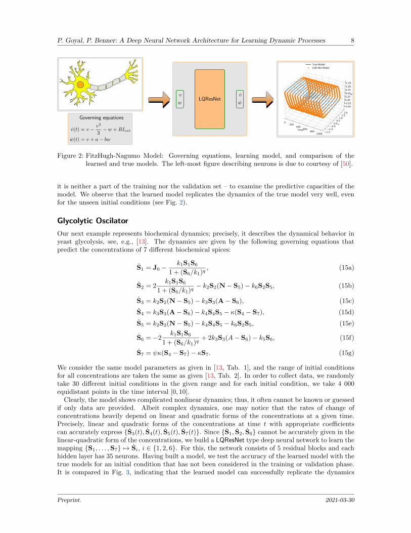
As a first example, we consider the FitzHugh-Nagumo model [17] that describes spiking of a neuron,neuronal dynamical in a simplistic way. The governing equations of such a dynamical behavior areshown in Fig. 2. The variables v(t) and w(t) describe activation and de-activation of a neuron. Specifi-cally, the model exhibits a periodic oscillatory behavior when Iext exceeds a threshold value. We collectdata by simulating the model using 10 randomly chosen initial conditions in the range [−1, 1]× [−1, 1],and for each initial condition, we collect 5 000 equidistant points in the time interval [0, 200]s. Hav-ing these data, we build two models that map {v(t), w(t)} 7→ v(t) and {v(t), w(t)} 7→ w(t). Beforebuilding a deep neural network, we determine the residual as shown in Eq. 7. As a result, we findthat w(t) can accurately be written in the linear and quadratic forms of {v(t), w(t)}; thus, we haveanalytical model for the mapping. On the other hand, the linear and quadratic forms of {v(t), w(t)}are not sufficient to represent v(t). Hence, we make use of the residual type neural network to learnthe mapping {v(t), w(t)} 7→ v(t) using two residual blocks and each hidden layer having ten neurons.Having trained the model, we test the learned model with the true model for an initial condition –



v

wLQResNet

v

w

Governing equations

v(t) = v − v3

3− w +RIext

w(t) = v + a− bw

Time

0200

400600

8001000

v

1.51.0

0.50.0

0.51.0

1.52.0

w

0.500.25

0.000.250.500.751.001.25

True ModelLQR-Net Model

Figure 2: FitzHugh-Nagumo Model: Governing equations, learning model, and comparison of thelearned and true models. The left-most figure describing neurons is due to courtesy of [50].

it is neither a part of the training nor the validation set – to examine the predictive capacities of themodel. We observe that the learned model replicates the dynamics of the true model very well, evenfor the unseen initial conditions (see Fig. 2).

Glycolytic Oscilator

Our next example represents biochemical dynamics; precisely, it describes the dynamical behavior inyeast glycolysis, see, e.g., [13]. The dynamics are given by the following governing equations thatpredict the concentrations of 7 different biochemical spices:

S1 = J0 −k1S1S6

1 + (S6/k1)q, (15a)

S2 = 2k1S1S6

1 + (S6/k1)q− k2S2(N− S5)− k6S2S5, (15b)

S3 = k2S2(N− S5)− k3S3(A− S6), (15c)

S4 = k3S3(A− S6)− k4S4S5 − κ(S4 − S7), (15d)

S5 = k2S2(N− S5)− k4S4S5 − k6S2S5, (15e)

S6 = −2k1S1S6

1 + (S6/k1)q+ 2k3S3(A− S6)− k5S6, (15f)

S7 = ψκ(S4 − S7)− κS7. (15g)

We consider the same model parameters as given in [13, Tab. 1], and the range of initial conditionsfor all concentrations are taken the same as given [13, Tab. 2]. In order to collect data, we randomlytake 30 different initial conditions in the given range and for each initial condition, we take 4 000equidistant points in the time interval [0, 10].

Clearly, the model shows complicated nonlinear dynamics; thus, it often cannot be known or guessedif only data are provided. Albeit complex dynamics, one may notice that the rates of change ofconcentrations heavily depend on linear and quadratic forms of the concentrations at a given time.Precisely, linear and quadratic forms of the concentrations at time t with appropriate coefficientscan accurately express {S3(t), S4(t), S5(t), S7(t)}. Since {S1, S2, S6} cannot be accurately given in thelinear-quadratic form of the concentrations, we build a LQResNet type deep neural network to learn themapping {S1, . . . ,S7} 7→ Si, i ∈ {1, 2, 6}. For this, the network consists of 5 residual blocks and eachhidden layer has 35 neurons. Having built a model, we test the accuracy of the learned model with thetrue models for an initial condition that has not been considered in the training or validation phase.It is compared in Fig. 3, indicating that the learned model can successfully replicate the dynamics



Dynamics of Glycolytic Oscillator

x = y

Figure 3: Glycolytic Oscillator: A comparison of true and learned model for an initial condition thatis not used for training. In red color (true model), and cyan dotted (learned model).

without any prior knowledge of the biochemical process or model. Moreover, we note that the learningprocess can be even more improved if a topological network describing the interconnection of speciesis known. To make it clearer, from Eq. 15, we have that the dynamics of S1 only dependent on S1,S6;hence, we need to feed only theses variables into a network to learn the dynamics of S1.

Discussion

In essence, we have discussed a compelling approach to learning complex nonlinear dynamical systemsusing data that can incorporate any prior knowledge of a process. The approach, in particular, makesuse of the observation, which is often found in dynamical systems’ modeling – that is, the rate ofchange of a variable strongly depends on linear and quadratic forms of the variable. Thus, we haveproposed an efficient deep learning architecture, LQResNet, that can be seen as a good compromisebetween purely interpretable mechanistic approaches and black-box neural network approaches. Theapproach can be employed in various fields, where abundant data can be obtained, where underlyingphysics or models describing dynamics are not completely known, for instance, in biological processmodeling, climate science, epidemiology, and financial markets. Moreover, there are various instanceswhere we have a fairly good understanding of the process, which may be derived from physical lawsor expert knowledge, but it fails to explain the data collection, for instance, in an experimental setup,due to some hidden dynamics or forces. Hence, the proposed methodology can be applied to learna correction term using LQResNet, by combining the knowledge of the process as well as data. As aresult, we expect to obtain a good model with a limited amount of data. We have demonstrated theefficiency of the proposed methodology to learning models using two examples arising in biology andbiochemistry. We have observed that these models generalize even to unseen conditions.

One of the current limitations of the approach is the need for accurate data that sufficiently approx-imates the derivative information. The derivative information is necessary to obtain a continuous-timedynamic model; however, this is challenging to attain from noisy measurements. Indeed, we may first



obtain a discrete-time model and then determine an approximate continuous-time model. However,as our future work, we intend to propose efficient deep learning approaches to obtain continuous-timemodels from noisy data by filtering the noise in the course of learning, though there are some advance-ments in the direction in [40]. In the future, we also aim at tailoring the approach to the case whendata is not collected at a regular time interval.

Code Availability

Our Python implementation using PyTorch is available online under the link

https://github.com/mpimd-csc/LQRes-Net.

References

[1] Peter Benner, Pawan Goyal, Jan Heiland, and Igor Pontes Duff. Operator inference and physics-informed learning of low-dimensional models for incompressible flows. arXiv:2010.06701, 2020.

[2] Peter Benner, Pawan Goyal, Boris Kramer, Benjamin Peherstorfer, and Karen Willcox. Opera-tor inference for non-intrusive model reduction of systems with non-polynomial nonlinear terms.Comp. Meth. Appl. Mech. Eng., 372:113433, 2020.

[3] Gal Berkooz, Philip Holmes, and John L Lumley. The proper orthogonal decomposition in theanalysis of turbulent flows. Annual Rev. Fluid Mech., 25(1):539–575, 1993.

[4] Josh Bongard and Hod Lipson. Automated reverse engineering of nonlinear dynamical systems.Proc. Nat. Acad. Sci. U.S.A., 104(24):9943–9948, 2007.

[5] Didier Bresch. Shallow-water equations and related topics. In Handbook of Differential Equations:Evolutionary Equations, volume 5, pages 1–104. Elsevier, 2009.

[6] Steven L Brunton, Joshua L Proctor, and J Nathan Kutz. Discovering governing equationsfrom data by sparse identification of nonlinear dynamical systems. Proc. Nat. Acad. Sci. U.S.A.,113(15):3932–3937, 2016.

[7] Emmanuel J Candes, Justin Romberg, and Terence Tao. Robust uncertainty principles: Exactsignal reconstruction from highly incomplete frequency information. IEEE Trans. Inform. Theory,52(2):489–509, 2006.

[8] Rick Chartrand. Numerical differentiation of noisy, nonsmooth data. ISRN Appl. Math., 2011,2011.

[9] Ricky TQ Chen, Yulia Rubanova, Jesse Bettencourt, and David K Duvenaud. Neural ordinarydifferential equations. In Advances Neural Inform. Processing Sys., pages 6571–6583, 2018.

[10] Djork-Arne Clevert, Thomas Unterthiner, and Sepp Hochreiter. Fast and accurate deep networklearning by exponential linear units (ELUs). arXiv preprint arXiv:1511.07289, 2015.

[11] James P Crutchfield and Bruce S McNamara. Equations of motion from a data series. ComplexSys., 1(417-452):121, 1987.

[12] Bryan C Daniels and Ilya Nemenman. Automated adaptive inference of phenomenological dy-namical models. Nature Comm., 6(1):1–8, 2015.

[13] Bryan C Daniels and Ilya Nemenman. Efficient inference of parsimonious phenomenological modelsof cellular dynamics using S-systems and alternating regression. PLoS One, 10(3):e0119821, 2015.


https://github.com/mpimd-csc/LQRes-Net


[14] David L Donoho. Compressed sensing. IEEE Trans. Inform. Theory, 52(4):1289–1306, 2006.

[15] Ronald Aylmer Fisher. The wave of advance of advantageous genes. Annals of Eugenics, 7(4):355–369, 1937.

[16] Richard FitzHugh. Mathematical models of threshold phenomena in the nerve membrane. TheBulletin Math. Biophys., 17(4):257–278, 1955.

[17] Richard FitzHugh. Impulses and physiological states in theoretical models of nerve membrane.Biophysical J., 1(6):445–466, 1961.

[18] R Gonzalez-Garcia, R Rico-Martinez, and IG Kevrekidis. Identification of distributed parametersystems: A neural net based approach. Computers & Chemical Engrg., 22:S965–S968, 1998.

[19] Ian Goodfellow, Yoshua Bengio, and Aaron Courville. Deep learning. MIT press, 2016.

[20] Kaiming He, Xiangyu Zhang, Shaoqing Ren, and Jian Sun. Deep residual learning for imagerecognition. In Proc. IEEE Conf. Comp. Vision Patt. Recog., pages 770–778, 2016.

[21] Holger Kantz and Thomas Schreiber. Nonlinear Time Series Analysis, volume 7. CambridgeUniversity Press, 2004.

[22] Ioannis G Kevrekidis, C William Gear, James M Hyman, Panagiotis G Kevrekidis, Olof Runborg,Constantinos Theodoropoulos, et al. Equation-free, coarse-grained multiscale computation: En-abling mocroscopic simulators to perform system-level analysis. Comm. Math. Sci., 1(4):715–762,2003.

[23] Diederik P Kingma and Jimmy Ba. Adam: A method for stochastic optimization. arXiv preprintarXiv:1412.6980, 2014.

[24] Alex Krizhevsky, Ilya Sutskever, and Geoffrey E Hinton. Imagenet classification with deep con-volutional neural networks. In Adv. Neural Inform. Processing Sys., pages 1097–1105, 2012.

[25] S Narendra Kumpati and Parthasarathy Kannan. Identification and control of dynamical systemsusing neural networks. IEEE Trans. Neural Networks, 1(1):4–27, 1990.

[26] Karl Kunisch and Stefan Volkwein. Galerkin proper orthogonal decomposition methods for ageneral equation in fluid dynamics. SIAM J. Numer. Anal., 40(2):492–515, 2002.

[27] Yann LeCun, Yoshua Bengio, and Geoffrey Hinton. Deep learning. Nature, 521(7553):436–444,2015.

[28] Hao Li, Zheng Xu, Gavin Taylor, Christoph Studer, and Tom Goldstein. Visualizing the losslandscape of neural nets. In Neural Inform. Processing Syst., 2018.

[29] Liyuan Liu, Haoming Jiang, Pengcheng He, Weizhu Chen, Xiaodong Liu, Jianfeng Gao, and JiaweiHan. On the variance of the adaptive learning rate and beyond. arXiv preprint arXiv:1908.03265,2019.

[30] Lennart Ljung. System Identification: Theory for the User. Prentice Hall, NJ, 1999.

[31] Shane A McQuarrie, Cheng Huang, and Karen Willcox. Data-driven reduced-order mod-els via regularized operator inference for a single-injector combustion process. arXiv preprintarXiv:2008.02862, 2020.

[32] Michele Milano and Petros Koumoutsakos. Neural network modeling for near wall turbulent flow.J. Comput. Phys., 182(1):1–26, 2002.



[33] Vidvuds Ozolins, Rongjie Lai, Russel Caflisch, and Stanley Osher. Compressed modes for varia-tional problems in mathematics and physics. Proc. Nat. Acad. Sci. U.S.A., 110(46):18368–18373,2013.

[34] Benjamin Peherstorfer and Karen Willcox. Data-driven operator inference for nonintrusiveprojection-based model reduction. Comp. Meth. Appl. Mech. Eng., 306:196–215, 2016.

[35] Joshua L Proctor, Steven L Brunton, Bingni W Brunton, and JN Kutz. Exploiting sparsity andequation-free architectures in complex systems. Europ. Phy. J. Spec. Top., 223(13):2665–2684,2014.

[36] E. Qian, B. Kramer, B. Peherstorfer, and K. Willcox. Lift & learn: Physics-informed ma-chine learning for large-scale nonlinear dynamical systems. Physica D: Nonlinear Phenomena,406:132401, 2020. URL: https://doi.org/10.1016/j.physd.2020.132401.

[37] Maziar Raissi, Paris Perdikaris, and George E Karniadakis. Physics-informed neural networks:A deep learning framework for solving forward and inverse problems involving nonlinear partialdifferential equations. J. Comput. Phys., 378:686–707, 2019.

[38] Clarence W Rowley, Igor Mezic, Shervin Bagheri, Philipp Schlatter, and Dans Henningson. Spec-tral analysis of nonlinear flows. J. Fluild Mech., 641(1):115–127, 2009.

[39] Samuel H Rudy, Steven L Brunton, Joshua L Proctor, and J Nathan Kutz. Data-driven discoveryof partial differential equations. Sci. Adv., 3(4):e1602614, 2017.

[40] Samuel H Rudy, J Nathan Kutz, and Steven L Brunton. Deep learning of dynamics and signal-noise decomposition with time-stepping constraints. J. Comput. Phys., 396:483–506, 2019.

[41] Hayden Schaeffer, Russel Caflisch, Cory D Hauck, and Stanley Osher. Sparse dynamics for partialdifferential equations. Proc. Nat. Acad. Sci. U.S.A., 110(17):6634–6639, 2013.

[42] Peter J Schmid. Dynamic mode decomposition of numerical and experimental data. J. FluildMech., 656:5–28, 2010.

[43] Michael D Schmidt, Ravishankar R Vallabhajosyula, Jerry W Jenkins, Jonathan E Hood, Ab-hishek S Soni, John P Wikswo, and Hod Lipson. Automated refinement and inference of analyticalmodels for metabolic networks. Phy. Biology, 8(5):055011, 2011.

[44] Johan AK Suykens, Joos PL Vandewalle, and Bart L de Moor. Artificial Neural Networks forModelling and Control of Non-Linear Systems. Springer, 1996.

[45] Robert Tibshirani. Regression shrinkage and selection via the lasso. J. Royal Stat. Soc.: SeriesB (Methodological), 58(1):267–288, 1996.

[46] Peter Van Overschee and Bart de Moor. Subspace Identification of Linear Systems: Theory,Implementation, Applications. Kluwer Academic Publishers, 1996.

[47] Wen-Xu Wang, Rui Yang, Ying-Cheng Lai, Vassilios Kovanis, and Celso Grebogi. Predicting catas-trophes in nonlinear dynamical systems by compressive sensing. Phy. Rev. Letters, 106(15):154101,2011.

[48] Matthew O Williams, Ioannis G Kevrekidis, and Clarence W Rowley. A data–driven approxi-mation of the Koopman operator: Extending dynamic mode decomposition. J. Nonlinear Sci.,25(6):1307–1346, 2015.

[49] Hao Ye, Richard J Beamish, Sarah M Glaser, Sue CH Grant, Chih-hao Hsieh, Laura J Richards,Jon T Schnute, and George Sugihara. Equation-free mechanistic ecosystem forecasting usingempirical dynamic modeling. Proc. Nat. Acad. Sci. U.S.A., 112(13):E1569–E1576, 2015.


https://doi.org/10.1016/j.physd.2020.132401


[50] Bin Zhen, Zhenhua Li, and Zigen Song. Influence of time delay in signal transmission on synchro-nization between two coupled FitzHugh-Nagumo neurons. Appl. Sci., 9(10):2159, 2019.


lqresnet: a deep neural network architecture for learning

Documents