IEEE SIGNAL PROCESSING MAGAZINE [117] JULY 2011

approximate formula for the 3-dB cutoff frequency as a function of polynomial order N and impulse response half-length M. Engineers with a frequency-domain mindset (like the author) may find this useful if they choose to use S-G filters in their application.

AUTHORRonald W. Schafer (ron.schafer@hp.com) is an HP Fellow in the Mobile and Immersive Experience Lab at HP Labs, Palo Alto, California, where he is involved in research on acoustic and audio signal processing. From 1974 to 2004, he was John and Marilu McCarty Professor of the School of Electrical and Computer Engineering at Georgia Tech. He is the

coauthor of several DSP textbooks includ-ing Discrete-Time Signal Processing (with Oppenheim), Signal Processing First (with McClellan and Yoder), and Theory and Applications of Digital Speech Processing (with Rabiner).

REFERENCES[1] K. Pandia, S. Revindran, R. Cole, G. Kovacs, and L. Giaovangrandi, “Motion artifact cancella-tion to obtain heart sounds from a single chest-worn accelerometer,” in Proc. ICASSP-2010, 2010, pp. 590–593.

[2] R. W. Schafer, “On the frequency-domain properties of Savitzky-Golay filter,” in Proc. 2011 DSP/SPE Workshop, Sedona, AZ, Jan. 2011, pp. 54–59.

[3] A. Savitzky and M. J. E. Golay, “Soothing and differentiation of data by simplified least squares procedures,” Anal. Chem., vol. 36, pp. 1627–1639, 1964.

[4] J. Riordon, E. Zubritsky, and A. Newman, “Top 10 articles,” Anal. Chem., vol. 72, no. 9, pp. 324A–329A, May 2000.

[5] M. Sühling, M. Arigovindan, P. Hunziker, and M. Unser, “Multiresolution moment filters: Theory and applications,” IEEE Trans. Image Processing, vol. 13, no. 4, pp. 484–495, Apr. 2004.

[6] M. U. A. Bromba and H. Ziegler, “Applica-tion hints for Savitzky-Golay smoothing filters,” Anal. Chem., vol. 53, no. 11, pp. 1583–1586, Sept. 1981.

[7] R. W. Ha mming, Digital Filters, 3rd ed. Englewood Cliffs, NJ: Prentice-Hall, 1989.

[8] S. J. Or fanidis. (1995–2009). Introduction to signal processing [Online]. Available: www.ece.rutgers.edu/~orfanidis/intro2sp

[9] P.-O. Pe rsson and G. Strang, “Smoothing by Savitzky-Golay and Legendre filters,” IMA Vol. Math. Systems Theory Biol., Comm., Comp., and Finance, vol. 134, pp. 301–316, 2003.

[10] W. H. Pr ess , S . A . Teukolsky, W. T. Vertterling, and B. P. Flannery, Numerical Recipes, 3rd ed. Cambridge, U. K.: Cambridge Univ. Press, 2007.

[11] A. V. Op penheim and R. W. Schafer, Discrete-Time Signal Processing, 3rd ed. Upper Saddle River, NJ: Pearson, 2010.

[SP]

In this article, the goal is to show that it is possible to filter non-u n i f o r m l y s a m p l e d s i g n a l s according to specs defined in the Fourier domain. In many practi-

cal applications, it is necessary to fil-ter irregularly sampled data including seismic signal processing, synthetic aperture radar (SAR) imaging sys-tems, three-dimensional (3-D) mesh-es, and digital terrain models [1], [2]. In almost all of these practical prob-lems, it is possible to define the desired filtering solution in a set the-oretic framework. This lecture note presents a new method for filtering irregularly sampled data by defining stopband tolerance regions in the Fourier domain and time-domain upper and lower bounds on the signal

samples as a part of the filtering pro-cess. Since there are specifications in both time and frequency domains, it is possible to iterate between time and frequency domains using the fast Fourier transform (FFT) while impos-ing the constraints in each domain.

RELEVANCEThe ideas presented here can be used to develop filtering algorithms for irregu-larly sampled one or higher dimension-al data. It can be used as a teaching material in advanced undergraduate and graduate discrete-time signal pro-cessing, optimization as well as applied mathematics courses.

PREREQUISITESThe prerequisites for understanding this article’s material are linear algebra, dis-crete-time signal processing, and basic optimization theory.

PROBLEM STATEMENTLet us assume that samples xc 1ti 2 , i5 0, 1, 2, c, L2 1, of a continuous time-domain signal xc 1t 2 are available. These samples may not be on an uni-form sampling grid. Let us define xd 3n 45 xc 1nTs 2 as the uniformly sam-pled version of this signal. We assume that the sampling period Ts is sufficient-ly small (below the Nyquist period) for the signal xc 1t 2 . In a typical discrete-time filtering problem, we have xd 3n 4 or its noisy version, and we apply a dis-crete-time low-pass filter to the uni-formly sampled signal xd 3n 4. However, xd 3n 4 is not available in this problem. Only nonuniformly sampled data xc 1ti 2 , i50, 1, 2, c , L21 are available in this problem.

GOALOur goal is to low-pass filter the non-uniformly sampled data xc 1ti 2 according

Kivanc Kose and A. Enis Cetin

Low-Pass Filtering of Irregularly Sampled Signals Using a Set Theoretic Framework

Digital Object Identifier 10.1109/MSP.2011.941098 Date of publication: 15 June 2011

1053-5888/11/$26.00©2011IEEE

IEEE SIGNAL PROCESSING MAGAZINE [118] JULY 2011

[lecture NOTES] continued

to a given cutoff frequency. One can try to interpolate available samples to the regular grid and apply a discrete-time filter to the data but this will amplify the noise because the available samples may be corrupted by noise [3]. In fact, only noisy samples are available in some problems [4].

PROPOSED SOLUTIONThe proposed filtering algorithm is essen-tially a variant of the well-known Papoulis-Gerchberg interpolation method [1], [5]–[10] and our earlier finite impulse response (FIR) filter design method [11]. The solution is based on the projections onto convex sets (POCSs) framework. In this approach, specifications in the time and frequency domain are formulated as sets and a signal in the intersection of constraint sets is defined as the solution, which can be obtained in an iterative manner. In each iteration, the FFT algo-rithm is used to go back and forth between the time and frequency domains.

In many signal reconstruction and band-limited interpolation problems [1], [5]–[7], Fourier domain information is represented using a set, which is defined as follows:

Cp5 5x : X 1ejw 2 5 0 for wc # w # p6, (1)

where X 1ejw 2 is the discrete-time Fourier transform (DTFT) of the dis-crete-time signal x 3n 4 and wc is the band-limitedness condition or the desired normalized angular low-pass cutoff frequency [1], [5], [6]. This con-dition is imposed on a given signal xo 3n 4 by orthogonal projection onto the set Cp as follows. The projection xp is obtained by simply imposing the frequency domain constraint on the signals

Xp 1ejw 2 5 eXo 1ejw 2 for 0 # w # wc

0 for w . wc ,

(2)

where Xo 1ejw 2 and Xp 1ejw 2 are the DTFTs of xo and xp, respectively. Members of the set Cp are infinite extent signals, so the FFT size should be large during the implementation of the projection on to the set Cp.

This approach is different from the Papoulis-Gerchberg type method [1], [5], [6] because it allows the signal to have some high-frequency components according to the tolerance parameter ds. The use of the stopband and the transition regions eliminates ringing artifacts due to the Gibbs phenomenon. We define another set corresponding to the stopband condition in the Fourier domain as follows:

Cs5 5x : |X 1ejw 2 | # ds for ws # w # p6, (3)

where the stopband frequency ws . wc. The set Cs is also a convex set [6], [12], and we can impose this condition on iterates during iterative filtering. We find a member xg of the set Cs corresponding to a given signal xo 3n 4 as follows:

Xg 1ejw 2 5 •Xo 1e jw 2 for 0 , w , ws

Xo 1e jw 2 for |Xo 1e jw 2 | # ds, w $ ws

dsejfo1w2 for |Xo 1e jw 2 | $ ds, w $ ws

,

(4)

where fo 1w 2 is the phase of Xo 1ejw 2 . Clearly, xg is in the set Cs. In our implementation, the set Cs plays the key role rather than the set Cp because almost all signals that we encounter in

543210

–1–2–3–4

543210

–1–2–3–4

–5100 200 300 400 500 600 700 800 900 1,000

100 200 300 400 500 600 700 800 900 1,000

(a)

(b)

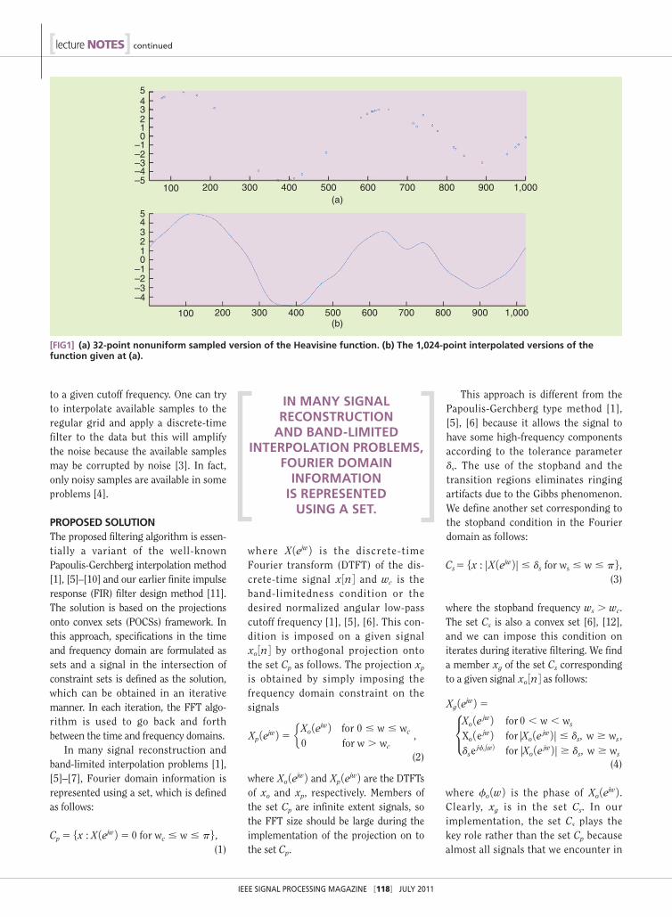
[FIG1] (a) 32-point nonuniform sampled version of the Heavisine function. (b) The 1,024-point interpolated versions of the function given at (a).

IN MANY SIGNAL RECONSTRUCTION

AND BAND-LIMITED INTERPOLATION PROBLEMS,

FOURIER DOMAIN INFORMATION

IS REPRESENTED USING A SET.

IEEE SIGNAL PROCESSING MAGAZINE [119] JULY 2011

practice are not band-limited signals. Most signals have some high-frequen-cy content. The frequency band 1wc, ws 2 corresponds to the transition band used in ordinary discrete-time filter design.

As pointed out above, we use a sam-pling period, which is smaller than the Nyquist period. Let us assume that 0, Ts, 2Ts, c, 1N2 1 2Ts is a dense grid

covering ti, i5 0, 1, 2, c, L2 1 and let us also assume that all ti , ti11 and ti $ 0 and tL21 # 1N2 1 2Ts without loss of generality. The set describing the time-domain information is defined using the regular sampling grid 0, Ts, 2Ts, c, 1N2 1 2Ts. Let us assume that the sample at t5 ti is close to nTs. We impose upper and lower bounds on x 3n 4 as follows:

xc 1ti 2 2 ei # x 3n 4 # xc 1ti 2 1 ei (5)

and the corresponding time-domain set is defined as

Ci5 5x : xc 1ti22ei# x 3n4# xc 1ti21ei6, (6)

where the time-domain bound parame-ter ei can be either selected as a constant value or as an a -percent of xc 1ti 2 in a

543210

–1–2–3–4–5

100 200 300 400 500 600 700 800 900 1,000

(a)

(b)

543210

–1–2–3–4–5

100 200 300 400 500 600 700 800 900 1,000

543210

–1–2–3–4–5

100 200 300 400 500 600 700 800 900 1,000(c)

[FIG2] (a) The Heavisine signal, (b) 256 Heavisine signal samples corrupted by additive Gaussian noise with variance s 5 0.3, and (c) 1,024 point restored signal using the samples given in (b).

543210

–1–2–3–4–5

100 200 300 400 500 600 700 800 900 1,000

First IterationTenth Iteration20th Iteration58th Iteration

[FIG3] Restored signals after 1, 10, 20, and 58 iteration rounds.

IEEE SIGNAL PROCESSING MAGAZINE [120] JULY 2011

[lecture NOTES] continued

practical implementation. Although we do not know the signal value at nTs on the regular grid, it should be close to the sample value xc 1ti 2 due to the low-pass nature of the desired signal. Therefore, we model this information by imposing upper and lower bounds on the discrete-time signal in sets Ci , i5 0, 1, 2, c, L2 1. Furthermore, samples may

be corrupted by noise and upper and lower bounds on sample values provide robustness against noise. If there are two signal samples close to x 3n 4, the grid size can be increased, i.e., the sampling period can be reduced so that there is one x 3n 4 corresponding to each xc 1ti 2 . Other time-domain constraints that can be used in an iterative algorithm include the positivity constraint x 3n 4 $ 0, if the signal is nonnegative, and the finite energy set

CE5 5x : ||x||2 # E6, (7)

which is introduced in [6] for band-lim-ited interpolation problems to provide robustness against noise.

ITERATIVE FILTERING ALGORITHMThe iterative filtering algorithm consists of going back and forth between time and frequency domains and imposing the time and frequency constraints on iterates. We start with an arbitrary initial signal xo 3n 4. We project it onto sets Ci by using the time-domain constraints defined in (5) and obtain the first iterate x1 3n 4. Next, we need to compute the DTFT of x1 3n 4 and impose the frequency domain constraint defined in (4) to obtain X2.

We then compute the inverse-DTFT of X2 to obtain x2. At this stage, other time-domain constraints such as positiv-ity and finite energy can be also imposed on x2, if the signal is known to be a non-negative signal. Once x2 is obtained, it probably violates the time-domain con-straints defined by inequalities (5). Therefore, x3 is obtained by imposing the constraints on x2. The iterates defined in this manner converge to a sig-nal in the intersection of the time-domain set Ci and the frequency domain set Cs, if they intersect. In other words,

1,200

1,000

800

600

400

200

0

220200

180160

140120

10080

6040

20 50 100 150 200 250 300 350 400200180

160140

120100

8060

4020 50 100 150 200 250 300 350 4

[FIG5] Reconstructed model using one fourth of the randomly chosen samples of the original model. The reconstruction parameters are wc 5 p/4, ds 5 0.03, and ei 5 0.01.

[FIG6] Reconstructed model using one eighth of the randomly chosen samples of the original model. The reconstruction parameters are wc 5 p/8, ds 5 0.03, and ei 5 0.01.

1,200

1,000

800

600

400

200

0

220200

180160

140120

10080

6040

20 50 100 150 200 250 300 350 400

[FIG4] The original terrain model. The original model consists of 225 3 425 samples.

1,200

1,000

800

600

400

200

0

220200

180160

140120

10080

6040

20 50 100 150 200 250 300 350 40000180

160140

120100

8060

4020 50 100 150 200 250 300 350 4

IEEE SIGNAL PROCESSING MAGAZINE [121] JULY 2011

we eventually find a low-pass filtered ver-sion of the signal xc 1t 2 on the regular grid defined by 0, Ts, 2Ts, c, 1N2 1 2Ts. If the intersection of the sets Ci and Cs is empty then either the bounds ei should be increased or the cutoff frequency ws should be increased.

The iterative algorithm is globally convergent regardless of the initial start-ing signal, xo 3n 4. The proof of conver-gence is due to the POCSs theorem [6], [7], because the sets Cs, Ci, and CE are all convex sets in l2. Successive orthogonal projections onto these sets lead to a solu-tion, which is in the intersection of Cs, Ci, and CE. Papoulis-Gerchberg type iter-ations jumping back and forth between time and frequency domains converge in a relatively slow manner. Convergence speed can be increased using the nonor-thogonal projection methods described in [6], [7], and [13].

NUMERICAL EXAMPLESFigure 1 demonstrates the use of the low-pass filtering method for Donoho’s Heavisine signal shown in Figure 2(a). Due to the edges, this signal has high-frequency content. Therefore neither the strict band-limited interpolation employ-ing the set Cp nor the use of spline inter-polation will produce satisfactory results for this signal as demonstrated in [3].

In Figure 1, the number of available samples of the Heavisine signal is 32. Available samples are shown in Figure 1(a). In this case, the cutoff frequency w5 12 #p # 11 2 /1024, stopband parame-ter, ds5 0.03, and the time domain bound parameter ei5 0.01. The restored signal is shown in Figure 2(b). The restored signal is similar to the signal obtained using the wavelet domain methods described in [3].

In Figure 2, we randomly chose 256 points from the Heavisine signal, and we estimate the underlying continuous-time signal at 1,024 uniformly selected instances, i.e., x 3n 4, n50, 1, 2, c ,1023. The available signal samples are corrupted by Gaussian noise with variance s5 0.3 as in [3]. Corrupted Heavisine signal samples are shown in Figure 2(b). The restored sig-nal using the sets Cs and Ci is shown in Figure 2(c). The cutoff frequency

w51 2 # p# 20 2 /1024, stopband para-meter ds5 0.03, and the time domain bound parameter ei5 0.05. The recon-struction result is comparable to the wave-let domain interpolation method described in [3]. It is possible to restore the main fea-tures of Donoho’s Heavisine signal.

Convergence of the iterative algo-rithm can be proved using the projec-tions onto the convex sets theorem [6], [7] because the set Cs and sets Ci are closed and convex sets. In Figure 3, restored signals after 1, 10, 20, and 58 iteration rounds are shown.

A two-dimensional (2-D) example is provided in Figures 4, 5, and 6. The origi-nal terrain model given in Figure 4 con-sists of 2253425 sample points. As a first example, we assumed that one-fourth of the samples of the original signal are available in a random manner. The 2-D signal shown in Figure 5 is recon-structed using the parameters wc5p/4, ds5 0.03, and ei5 0.01. In the second example, we assume that one eighth of the samples of the original signal are available in a random manner. The recon-structed signal using the parameters wc5p/8, ds5 0.03, and ei5 0.01 is shown in Figure 6. Reconstruction results, which are given in Figures 5 and 6, are low-pass filtered versions of the original 2-D signal in a dense 2-D grid.

CONCLUSIONSIt is shown that it is possible to filter a nonuniformly sampled signal by using the stopband region in the Fourier domain. The filtering concept can be easily extended to bandpass, bandstop, and high-pass filtering. Rather than defining the passband region, desired stopband regions should be defined and used in the iterative filtering process. Moreover, as a byproduct, the method

can also be used for interpolating irregu-larly sampled data into a regularly sampled grid. In standard Papoulis-Gerchberg signal interpolation frame-work, high-frequency components are forced to take zero values. In our case, high-frequency values of the signal are allowed to take values according to stop-band condition defined in (3).

AUTHORSKivanc Kose (kkivanc@ee.bilkent.edu.tr) is a Ph.D. student at Bilkent University. His research interests are digital image, video, and 3-D signal processing. He is a Student Member of the IEEE.

A. Enis Cetin (cetin@bilkent.edu.tr) is a professor at Bilkent University. His main research interests are multimedia signal processing and its application. He is a Fellow of the IEEE.

REFERENCES[1] D. Munson, Jr. and E. Ullman, “Support-limited extrapolation of offset Fourier data,” in Proc. IEEE Int. Conf. Acoustics, Speech, and Signal Process-ing (ICASSP’86), vol. 11, Apr. 1986, pp. 2483–2486.

[2] A. Ozbek, “Noise filtering method for seismic data,” U.S. Patent 5 971 095, June 23, 1998.

[3] H. Choi and R. Baraniuk, “Interpolation and denoising of nonuniformly sampled data using wavelet-domain processing,” in Proc. IEEE Int. Conf. Acoustics, Speech, and Signal Processing (ICASSP), 1999, vol. 3, pp. 1645–1648.

[4] A. Ozbek, “Adaptive seismic noise and interfer-ence attenuation method,” U.S. Patent 6,651,007, Nov. 18, 2003.

[5] A. Papoulis, “A new algorithm in spectral analysis and band-limited extrapolation,” IEEE Trans. Cir-cuits Syst., vol. 22, no. 9, pp. 735–742, Sept. 1975.

[6] D. C. Youla and H. Webb, “Image restoration by the method of convex projections: Part 1 theory,” IEEE Trans. Med. Imag., vol. 1, no. 2, pp. 81–94, Oct. 1982.

[7] P. Combettes, “The foundations of set theoretic estimation,” Proc. IEEE, vol. 81, no. 2, pp. 182–208, Feb. 1993.

[8] H. J. Trussell and D. M. Rouse, “Reducing non-zero coefficients in FIR filter design using POCS,” in Proc. European Signal Processing Conf. (EU-SIPCO), Sept. 2005.

[9] W. Lertniphonphun and J. McClellan, “Complex frequency response FIR filter design,” in Proc. 1998 IEEE Int. Conf. Acoustics, Speech and Signal Pro-cessing, May 1998, vol. 3, pp. 1301–1304.

[10] K. Haddad, H. Stark, and N. Galatsanos, “Con-strained FIR filter design by the method of vector space projections,” IEEE Trans. Circuits Syst. II, vol. 47, no. 8, pp. 714–725, Aug. 2000.

[11] A. Cetin, O. Gerek, and Y. Yardimci, “Equiripple FIR filter design by the FFT algorithm,” IEEE Sig-nal Processing Mag., vol. 14, no. 2, pp. 60–64, Mar. 1997.

[12] A. E. Cetin and R. Ansari, “Convolution-based framework for signal recovery and applications,” J. Opt. Soc. Am. A, vol. 5, no. 8, pp. 1193–1200, 1988.

[13] K. Slavakis, S. Theodoridis, and I. Yamada, “On-line kernel-based classification using adaptive projec-tion algorithms,” IEEE Trans. Signal Processing, vol. 56, no. 7, pp. 2781–2796, July 2008. [SP]

THE ITERATIVE FILTERING ALGORITHM CONSISTS OF GOING BACK AND FORTH

BETWEEN TIME AND FREQUENCY DOMAINS AND

IMPOSING THE TIME AND FREQUENCY CONSTRAINTS

ON ITERATES.