low-frequency variability of the the purposeful study … · the purposeful study of the...
TRANSCRIPT
IILow-FrequencyVariability of theSea
Carl Wunsch
11.1 Introduction
The purposeful study of the time-dependent motion ofthe sea having periods longer than about 1 day is com-paratively recent. In the classic Handbuch of the early1940s, Sverdrup, Johnson, and Fleming (1942), onesearches in vain for more than the most peripheralreference to temporal changes on the large scale (oneof the few examples is their figure 110 showing theCalifornia Current at two different times). Until veryrecently, the ocean was treated as though it had anunchanging climate with no large-scale temporal var-iability. The reason for this is compelling and plain:until the electronics revolution of the past 30 years,the major oceanographic observational tool was theNansen bottle; using slow, uncomfortable ships, ittook essentially 100 years to develop a picture of thegross characteristics of the mean ocean. The more re-cent period, 1947 (Sverdrup, 1947) through about 1970(Stommel, 1965; Veronis, 1973b; and see chapter 5),was one of the intensive development of the theory oflarge-scale, steady models of the ocean circulation. Themethods were initially analytic, later numerical. Mostof these models were essentially low-Reynolds-num-ber, steady, sluggish, sticky, climatic oceans. In them,the role (if any) of small-scale, time-dependent proc-esses is simply parameterized by a positive eddy coef-ficient (Austauch) implying a down-the-mean-gradientflow of energy, momentum, heat, etc. The westward-intensification theories (Stommel, 1948; Munk, 1950)imply that any strong influence of such eddy coeffi-cients would be confined to the western boundariesand could be ignored in the interior ocean, except pos-sibly in the immediate vicinity of the eastward-movingfree-jet "Gulf Stream" (see Morgan, 1956). The result-ing models bear a remarkable resemblance to many ofthe gross features of the large-scale mean ocean circu-lation (see chapter 5).
The culmination of these analytic and numericalmodels of the large-scale circulation coincided with anumber of developments that ultimately underminedthe momentary confidence that the models representedthe correct dynamics of the ocean circulation. Thesedevelopments were of two kinds-instrumental andintellectual.
By 1970 instruments had been developed that madeit possible to obtain time-series measurements in theopen sea for periods far longer than a ship could pos-sibly remain in one location. These instruments in-cluded moored current meters, drifting neutrally buoy-ant floats, pressure gauges, and many others (Gould,1976; and see chapter 14). An additional "instrument"was the computer, which made it possible both tohandle the large data sets generated by time-series in-
342Carl Wunsch

struments and to explore new ideas by nonanalyticmeans. This computer impact has been felt, of course,in most branches of science.
The intellectual developments that shifted the focusfrom the mean circulation to the time-dependent partwere also of various kinds. The analytic models seem-ingly had reached a plateau at which their increasinglyintricate features [e.g., essentially laminar boundarylayers of higher and higher order as in Moore and Niiler(1975)] seemed untestable and intuitively implausibleoutside the laboratory. Physical oceanography is alsoto some extent a mirror of meteorology; by 1970 mostoceanographers were at least vaguely familiar with thepicture of the atmosphere that had emerged over theprevious decades. In that fluid system, the view of therole of eddies had shifted from a passive means ofdissipating the mean flows (through purely down-gra-dient fluxes of momentum, energy, etc.) to a muchmore interesting and subtle dynamic linkage in whichthe mean flows (the climate) were in at least someparts of the system driven by the eddy fluxes (Jeffreys,1926; Starr, 1968; Lorenz, 1967). Because many of themeteorological results would apply to any turbulentfluid, there was reason to believe that the ocean couldalso exhibit such intimate dynamic linkages. But weshould note that even now much work is still directedat studying the mean circulation by essentially classi-cal (though improved) means, as if the variability werenot dynamically important (e.g., Schott and Stommel,1978; Wunsch, 1978a; Reid, 1978). The extent to whichsuch pictures of the mean circulation of the large-scaletracers will survive complete understanding of varia-bility dynamics is not now clear.
In this chapter we shall review what is known aboutthe variability of the ocean. The expression "low-fre-quency variability," which is part of the title of thischapter, is a vague one used in a variety of ways byoceanographers, and encompassing a wide range ofthings. Here we mean by it anything with a time scalelonger than a day out to the age of the earth, althoughwe cannot really study by instrumental means phe-nomena with time scales longer than about 100 years.In spatial scale, it means phenomena ranging fromsome tens of kilometers to the largest possible globalocean oscillations. We shall, in common with recentpractice, also refer to the "eddy" field in the ocean.This word is often prefixed by "mesoscale" and is usedloosely to denote the subclass of variability encom-passing motions occurring on scale of hundreds of kil-ometers with time scales of months and longer. It is aconvenient shorthand and is meant to imply neitherany particular dynamics nor only flows with closedstreamlines. (The equivalent Soviet term is "synopticscale").
There is little doubt that oceanographers were quiteaware, from the very beginning, of time variability inthe ocean. Maury (1855, p. 358) remarked that in draw-ing his charts he had disregarded "numerous eddiesand local currents which are found at sea." He alsonotes in particular (p. 188) the highly variable equato-rial currents of the Pacific Ocean. Even earlier, Rennel(1832) had quoted another observer (C. Blagden), asreferring to North Atlantic currents as "casual" (Swal-low, 1976).
Most of the astute observers who worked at sea sinceMaury were very conscious of the difficulties of draw-ing conclusions about the mean circulation in the pres-ence of a highly time-dependent field. Figure 11.1,taken from Helland-Hansen and Nansen (1909), clearlydepicts what one suspects to be a time-dependent eddyfield. Sverdrup et al. (1942) make the statement thatdetermining the mean is difficult in the presence ofthe time variations, and that the closer the stationpairs are together, the greater is the requirement ofsimultaneity in hydrographic measurements. This is,of course, a statement about the frequency-wavenum-ber character of the baroclinic variability.
It is possible to give many instances of references toocean variability and eddies throughout the history ofobservational oceanography. But it is also fair to say
Figure II.I Chart of Norwegian Sea surface currents as con-structed by Helland-Hansen and Nansen (1909); reproducedby Sverdrup et al. (1942). One presumes the small-scale cur-rents are in fact time-dependent features.
343Low-Frequency Variability of the Sea

that little attention was paid to the phenomenon perse; it was a nuisance-a noise-contaminating deter-mination of the time mean flow. There are some majorexceptions, including Pillsbury's (1891) heroic effortsin the Florida Current, the 400-page work by Helland-Hansen and Nansen (1920), and somewhat later, Ise-lin's (1940a) attempts at monitoring the western NorthAtlantic. The question of the physical significance ofa weak mean flow in the presence of strong variabilityhas rarely been addressed even now.
11.1.1 Early TheoryThe first theoretical attempts to study the purely time-dependent oceanic motions at low frequency seem tobe outgrowths of the papers by Rossby and collabora-tors (1939) and by Haurwitz (1940a). These two studies,while directed primarily at the atmosphere, nonethe-less addressed themselves to the large-scale time-de-pendent wave motions of a rotating hydrostatic fluid-a characterization applying equally well to the ocean.The Rossby paper in particular introduced the /3-planeapproximation. These early efforts, and the large num-ber that followed, examined the wave motions knownmuch earlier. Indeed Laplace (1775) had discussed mo-tions that we now would call Rossby or planetarywaves (or in Hough's terminology, "tidal motions ofthe second class"). The study of these motions has along and distinguished history (e.g., Darwin, 1886; Ray-leigh, 1903; Poincar6, 1910), culminating in Hough's(1897, 1898) remarkable study of the solutions of theLaplace tidal equations on a sphere. [Lamb (1932), inhis chapter on tides gives a good summary of this work.He also thoroughly discusses (§206 and §212) what wecall "topographic Rossby waves" in which topographicgradients play a role analogous to the variation of theCoriolis parameter with latitude on a sphere.]
But it was Rossby's /3-plane that demonstrated thephysics in the simplest form and permitted an escapefrom the geometrical complexities of spherical coor-dinates. Arons and Stommel (1956), Veronis and Stom-mel (1956), Rattray (1964), Rattray and Charnell (1966),and others made explicit attempts to understand thepossible role of Rossby waves in the ocean. Longuet-Higgins in a series of papers (1964, 1965) justified the/3-plane approximation and carried out a modern ex-haustive search of the solutions on a sphere for a com-plete range of parameters far beyond what Hough coulddo in his time (Longuet-Higgins, 1968a, Longuet-Hig-gins and Pond, 1970). Most of this work was done inthe absence of any direct observational base in theocean. (For further discussion of these waves, see chap-ters 10 and 18).
Observations, which will be discussed at length be-low, suggest that linear wave models are inadequate to
describe much of the actual time-dependent motion inthe ocean. Nonetheless, as in the atmosphere (Holton,1975), many of the features of the observations arequalitatively similar to those deducible from the lineartheories. That is, the physics is modified by the non-linearity, but many of the linear features persist intothe nonlinear range. The precise extent to which thisis true is a function of the periods and spatial scales ofthe motions and is not really understood. As a gener-alization, it may be safe to assert that the largestoceanic scales of fluctuation are most likely to be dom-inated by linear dynamics. A linear description be-comes increasingly doubtful for smaller scales, and bar-otropic motions ought to be more nearly linear thanbaroclinic ones (Rhines, 1979).
The postulate of a time-dependent field in the inte-rior ocean immediately calls into question (Stommel,1965, p. 221) one of the fundamental deductions of thesteady-ocean models-that a Sverdrup balance appliesin the interior ocean.
Consider, for example, Stommel's (1948) model of ahomogeneous flat-bottom ocean on a i-plane. Let iq0 bethe time-mean transport streamfunction and let Pq, bethe time-dependent part. Then the time average vor-ticity balance may be written
J(V2q,0, 0) + (1Vq 1, q 1 ))
+ ,/3dq- + RV2ro = -VxT,ax (11.1)
where the bracket denotes a temporal average, VxTis the vertical component of the mean wind-stress curl,J denotes the Jacobian operator, and R is the coefficientof bottom friction. Let us assume that the mean fieldvaries over scales of 104 km, and that the time-depend-ent eddy field varies over 102 km. Let both the meanflows and the time-dependent part have magnitude10 cms - 1. Scaling, we obtain roughly, in nondimen-sional form,
10- 4 V21p0 + -x + 10-31(V20 ' S°0 )
ax
+ 10=1((V2qpl, 1)) = -kVX. (11.2)
Away from the western wall, the first term is negligi-ble; hence if we ignore both nonlinear terms, an inte-rior balance is
(11.3)dx_ = -Vx,ax
which is the conventional Sverdrup balance. But thenonlinear term
(11.4)
will be of the same order as the Sverdrup terms if the
344Carl Wunsch
11---.---111-1 �11 -b�_lllll _I .__�L________IL____L__11__�__1. �
01((V2q,, q/))
correlation in the bracket is no greater than 0.1, andhence the Sverdrup balance would be upset. The. easewith which one could destroy the simple relation (11.3)has motivated many of the recent studies of mesoscaleeddies. It is fair to state, however, that we are still notin a position to compute terms like (11.4) (or compa-rable terms in more sophisticated models) with suffi-cient accuracy to assess the adequacy of the Sverdruprelation. There is some evidence (Leetmaa, Niiler andStommel, 1977) that (11.3) is qualitatively correct awayfrom the eddy-rich area near the Gulf Stream itself, butno quantitative assessment has yet been possible. Onewould anticipate, based upon the known wide varia-bility in eddy energy levels (see discussion below) thatthere is a wide geographical variability in (11.4).
Constructs such as equation (11.2), which suggestthat eddies may be important in the open sea, are, ineffect, a reopening of the question that appeared tohave been answered by Stommel (1948) and Munk(1950), where the first-order effects of eddies-in theguise of eddy viscosities-were confined to the westernboundaries of the ocean. Webster (1961a, 1965), follow-ing Starr's lead, showed that at least in some regionsthe sign of the eddy flux of momentum might be op-posite to that assumed in the viscous models, and nowwe are at the stage of being unsure even whether theregional confinement to the west, which had seemedso clear in 1950, is valid.
Equation (11.2) and more realistic formulations im-ply that an energetic eddy field could upset the lowest-order open-ocean mean-vorticity balance. But eddiesalso can carry mass, momentum, heat, and other var-iables. It is not difficult to show the potential impor-tance and confusion that can arise from the presenceof a strong time-dependent flow field possessing smallscales. A simple example was presented by Longuet-Higgins (1969c), who considered a weakly nonlinearwave. In the weak-interaction limit, one can write thetime-mean particle velocities as
(U.) = (UL) + (Us),
where UE is the Eulerian velocity, UL the Lagrangianvelocity, and Us the Stokes velocity, which derivesfrom the wave Reynolds stresses. The Eulerian velocityis the value that would be measured by a current meterat a fixed point; the Lagrangian velocity would bemeasured by tracking a dyed particle. In the absence ofimposed exterior flows, Longuet-Higgins (1969c) dem-onstrated that the Eulerian and Lagrangian flows neednot have the same magnitude or direction, and indeedcan yield values differing by 180°. In the highly nonlin-ear limit it can be extremely difficult to find any simplerelation between the Eulerian and Lagrangian flowfields. Such possibilities call into question the entirenotion that there is some unique "general circulation"
of the ocean. Presumably one must carefully define thequantity whose overall circulation is desired, be it heat,mass, momentum, energy, passive tracer, etc., and seekthe dynamic balance that will govern its flux. Doingthis represents one of the most important problemsfacing oceanographers, who only recently have cometo grips with the existence of oceanic time variability.One anticipates that over the next decade the problemwill be solved, but it is impossible at the present timeto perceive the details of the actual dynamic and ki-nematic balances in the ocean.
In the past, there have been some attempts to studyspecial situations in which time variability was mod-eled in simple ways in order to seek an understandingof its potential role in the mean circulation. In partic-ular, Pedlosky (1965c), Veronis (1966c), and Munk andMoore (1968) all examined the possible role of weaklynonlinear Rossby waves in generating large-scale meanflows. All of these models used an Eulerian frame; asnoted above, obtaining an Eulerian means does notnecessarily imply the presence of an actual net watermovement. Often one can demonstrate the actual im-possibility of a Lagrangian mean (e.g., Moore, 1970) andthe question often hangs on subtle questions of dissi-pation (Eliassen and Palm, 1960; Charney and Drazin,1961) and the existence of critical levels (Andrews andMcIntyre, 1978a).
11.1.2 More Recent TheoryMany of the second-order effects of linear Rossby-wavemotions have been studied. Longuet-Higgins and Gill(1967), Lorenz (1972), Kim (1978), and Jones (1979) haveshown that the waves themselves are unstable. Thescattering of the waves by random currents was ex-amined by Keller and Veronis (1969), and scatteringfrom topography was studied by Hall (1976) amongothers. McKee (1972) examined the diffraction limit ofthe waves. Interaction of Rossby waves with meanshears has been studied primarily in a meteorologicalcontext by Charney and Drazin (1961), Holton 1975,chapter 4), and finite-amplitude waves in steady flowswere analyzed by Pedlosky (1970).
Finite-amplitude "soliton" solutions have been con-structed by Flierl (1979b) and Redekopp (1977) as aneffort to model the extreme form of ocean variabilityrepresented by Gulf Stream rings. These models haveusually been based upon some form of Korteweg-deVries equation and share many of the same propertiesas other known solitary waves (Whitham, 1974, chap-ters 16, 17; also see chapter 18, this volume).
Partly in response to the observational data base,which suggests that linear dynamics cannot be whollyadequate, there is a recent and growing literature ofthe opposite extreme, that is, based on the assumptionof a completely turbulent motion. In the weak-inter-action theories of Rossby waves (e.g., Longuet-Higgins
345Low-Frequency Variability of the Sea

and Gill, 1967) the energy transformation of a waveoccurs on a time scale long compared to a wave period.In the turbulence models, this is no longer true; theinteractions are rapid and strong and one is forced intoa statistical framework. An important step was takenby Chamey (1971a), who showed that "geostrophic tur-bulence" in a stratified fluid would behave much likestrictly two-dimensional turbulence known in othercontexts (Fj0rtoft, 1953; Kraichnan, 1967). This followsfrom the requirement that the fluid satisfy two inde-pendent quadratic constraints-conservation of energyand conservation of potential vorticity (enstrophy).
These ideas have been much elaborated since then(Rhines, 1979; Holloway and Hendershott, 1977;Salmon, Holloway, and Hendershott, 1976; Salmon,1978). The problems are subtle and difficult and thedominant mechanisms not yet completely sorted out.Numerical experiments have been done to study sev-eral different physical processes that can govern theevolution of given initial conditions. The pure baro-tropic nonlinear cascade process moves energy towardlarger spatial scales. Another nonlinear process trans-fers baroclinic energy toward the Rossby radius of de-formation and thence to the barotropic mode. Topo-graphic influences can scatter energy toward eitherlarger or smaller scales, depending upon the wavenum-ber spectrum of the initial conditions and of the bottomtopography. The relative importance of each of theseprocesses depends on the energy level and spatial struc-ture of the initial conditions. The balances are oftensubtle and no single process seems to dominatethroughout the plausible range of initial conditions.
The advent of observations of mesoscale motions inthe early 1970s also stimulated attempts to make nu-merical oceanic general-circulation models that couldresolve an interior eddy field rather than parameteriz-ing it simply as a constant, positive eddy viscosity. Byrestricting the calculations to limited ocean areas, itwas possible to have many forms of time variabilityappear explicitly in the models (Holland and Lin,1975a,b; Robinson, Harrison, Mintz, and Semtner,1977). As computers have become larger and faster, themodels have become ever more complex and realistic,including all of the physical mechanisms of the sim-pler-process models. However, it is fair to say that eventhe most sophisticated models now extant cannot fullymodel all of the observed physical complexity of theocean (Schmitz annd Owens, 1979). But this is not todenigrate the models. They are beginning to show qual-itatively many of the observed features of the oceansand doubtless rapidly will become much more realistic.Nonetheless, the ocean is very complex; numericalmodels that are intended to be realistic need also to becomplex. As more and more physics is added to thecomputer codes the results become increasingly diffi-
cult to understand. Indeed it may be that understandinga fully realistic numerical model of the ocean requiresnearly as much time, effort, and ingenuity as under-standing the real ocean.
We shall not dwell further here on the modem the-ories because there have been a number of recent re-views of the state of the art. Rhines (1977, 1979) hasdiscussed many of the basic ideas; the numericalmodels have been examined and compared by Robin-son, Harrison, and Haidvogel (1979) and Harrison(1979b). As we proceed to discuss the observations, weshall introduce additional theoretical hypotheses asneeded.
11.2 The Field of Variability of the Ocean
Perhaps the most sweeping generalization that can bemade about the known time variability in the ocean isthis: the ocean is filled with time-varying features,with all space and time scales, whose energy levelsvary by orders of magnitude over the ocean basins. Tostate it slightly differently, the field of variability islocally representable by a continuous frequency-wave-number spectrum; but the underlying process is notspatially stationary in the statistical sense and thisvitiates much of the utility of the spectral description.The use of the word "continuous" for the spectrum isdeliberate. Through much of the history of oceanog-raphy, as in many fields, there has been a search forsimple line processes, "cycles," which simply do notexist.
We know from the past decade of observation thatsimple universal parameterizations of the variabilityare not valid. The upper ocean is different (at leastsuperficially) from the lower ocean and the gyre centersare different from the gyre boundaries. Eastern wallsdiffer in their variability from western walls. It is prob-ably also true that the dynamics, as well as the kine-matics, of these regions differ. At this time, it is diffi-cult to give more than a fragmentary picture of open-ocean low-frequency variability because our observa-tional tools are still not adequate for the job of meas-uring a global ocean.
11.2.1 The Meteorological Forcing FunctionThe ocean is driven by the heating of the atmosphereand by direct momentum transfer from the winds. Thedetails of these processes are not completely clear (e.g.,Phillips, 1977a; Kraus, 1977), involving as they dosmall-scale turbulent transfer processes within themarine atmospheric and oceanic boundary layers.Nonetheless it is probable that the larger scales of theseforcing functions are able to communicate themselvesfrom the atmosphere to the ocean. That is, the detailsof the transfer of momentum to the ocean from the
346Carl Wunsch
-

A - GAN, MALDIVE IS.B --- BERMUDAC --- HILO, HAWAII
10-2 10-1FREQUENCY (cpd)
100
ITONI
>-I-Z ¢3 zwaz ,1Wa
= E
z0
W
o10
105
104
10-3
A -B ----
GAN, MALDIVE IS.BERMUDAHILO, HAWAIICANTON
I I I
10-2 10-1FREQUENCY (cpd)
100
Figure I I.zA Zonal wind spectra fromopen-ocean islands.
a few representative Figure II .Blands.
Meridional wind spectra from open-ocean is-
winds involves such small-scale processes as ordinaryripples, but we anticipate that if the wind varies overa 1000-km scale, then it is this variability scale that isrelevant to understanding the oceanic response towinds, and it is thus meaningful to seek a descriptionof the forcing function in frequency-wavenumberspace.
It is comparatively easy (Wunsch and Gill, 1976;Philander, 1978) to show that direct atmospheric-pres-sure forcing is a very inefficient process compared towind-stress forcing. Direct thermal forcing is likelyalso (Frankignoul and Miller, 1979) to be compara-tively weak except on the very largest time scales thatdetermine the mean thermohaline general circulation.
The description of how the atmosphere forces theocean is of considerable interest in studying the fieldof variability, but it may not be a decisive factor. Thereason is that theoretically one can drive oceanic var-iability indirectly through instabilities of the strong"mean" current systems (Lipps, 1963), and of the in-terior ocean (Gill, Green, and Simmons, 1974; Robin-son and McWilliams, 1974). Nonetheless in some re-gions at least-the continental shelves (see chapters 7and 10), in the open sea far from intense currents(Brown et al., 1975) and in regions like the FloridaCurrent (Diiing, Mooers, and Lee, 1977; Wunsch andWimbush, 1977)-there does seem to be some directresponse to atmospheric forcing, although it seems tobe at the short-period end of the spectrum, namely,periods shorter than about 10 days.
Some representative wind spectra are displayed infigure 11.2. It should be noted that stress is usually
en
I-
U)zW
10 1-zW
10-2
ZONAL WAVENUMBER
Figure I I.C Estimated wavenumber spectnim of meridionalgeostrophic wind at 30°N (heavy line) and 50°N (light line) fortwo frequencies at 1000 mb. Notice steep slope at high wave-numbers. Frankignoul and Miller, 1979.)
347Low-Frequency Variability of the Sea
IU
I-nU3zhJC3
UZI
N
Z
z0N
106
104
B-
C-
103I I
,7_7
A
106 _
_ _
10-3103 __

computed from the two winds components, (wx, w,) bythe formula
(T7,,7) = C(w + W2)¶2(w, W.,), (11.5)
where C is a parameter depending upon the drag coef-ficient and which in general (Bunker, 1976) dependsupon the air-sea temperature difference and possibly,upon the wind speed itself. But the spectrum of stresswill strongly resemble that of the wind because theexpression (11.5) preserves the zero crossings of thewind components. The spectrum is distorted relativeto that of the wind by the amplitude modulation factor(w + w2) " 2.
The spectra tend to become white (or less red) atperiods longer than a few days, reflecting the unpre-dictability of weather (by linear methods at least), andthen redden again at the longer and here unresolved)periods (but see figure 11.9A). The spectra show a greatvariety of geographical effects, viz., latitude changes,proximity to continental influences, topography (theHilo spectrum in particular seems greatly affected bythe presence of high mountains, being highly aniso-tropic at low frequency), and sea-land contrasts. In themid-latitude spectra, most of the energy is found in the4-10-day band characteristic of the weather systems.At periods longer than those displayed, the wind spec-tra tend to become white (see Willebrand, 1978). Fran-kignoul and Muller (1978) have computed estimates ofthe 1000-mb zonal wavenumber spectra for a varietyof latitudes, displayed here in figure 11.2C. One seesa distinct concentration in the low wavenumber bands.Extrapolation to the sea surface is not straightforward,however.
The response of the ocean to forcing by fluctuatingwind fields has been considered by Phillips (1966),Frankignoul and Mfiller (1979), Leetmaa (1978), andHarrison (1979a) in the period range of days to months.Although the final word has not been spoken, it appearsthat over most of the ocean direct wind forcing is un-likely to compete with internal instability processes.The weak seafloor pressure fluctuations measured byBrown et al. (1975) are spatially coherent on the largescale only at periods of 10 days and shorter, wherecurrent meter records show very little energy. Thesemay in fact be wind-forced barotropic modes but theyare energetically unimportant. In what follows thereader may want to compare the shape of the windspectra displayed in figure 11.2 with those of the othervariables discussed later.
Frequency spectra of atmospheric-pressure fluctua-tions (not shown) also tend to show a whitening at lowfrequency although Madden and Julian (1972) and Lu-ther (1980) have found some large-scale organized mo-tions at long periods, circa 50 days.
Sea-level measurements of atmospheric variabilityare sparse and inadequate for making definitive state-ments. Frankignoul and Miiller (1979) attempted toconstruct a model spectrum by synthesizing the avail-able data. They assumed spatial homogeneity and iso-tropy in the wind field. The two assumptions are ul-timately untenable, but their model is probably thebest that can be constructed at the present time.
11.2.2 Interannual Fluctuations in the OceanThese are changes with periods longer than 1 year. Ourmajor emphasis will be on those motions deduced inthe modem era of instrumentation, excluding periodsaccessible only through essentially geological methods.Thus with one exception (see below) we will not treatwhat is best called paleo-oceanography, which deservesa full treatment by itself.
Before attempting to describe what is known aboutthe very long-period changes in the ocean, there aretwo points to be made. Consider first figure 11.3. Figure11.3A is a section made by the vessel Challenger fromNew York to Bermuda to St. Thomas, Virgin Islands,in 1873. The figure at bottom is a section from theGrand Banks to Bermuda to the Mona Passage obtainedin 1954 and 1958 (Fuglister, 1960). The qualitative re-semblance is very close; clearly the fundamental as-sumption of large-scale physical oceanography-that atleast some aspects of the overall circulation, in partic-ular the large-scale baroclinic structure, have remainedstable for 100 years-is correct. That is consistent withthe statement of Sverdrup et al. (1942) noted aboveabout combining nonsimultaneous stations if they aresufficiently widely spaced, and is a (usually) unstatedassumption in discussions of the mean fields to thisday. It is well justified, for example, by comparing thehigh-quality Meteor sections in the South Atlanticmade in 1925-1927 and reported by Wiist and Defant(1936) with those made in 1954-1958 and reported byFuglister (1960). One is hard pressed to detect any sig-nificant differences on the large scale. (Of course, fromthese data one is able to say nothing regarding baro-tropic changes.)
One result of the paleo-oceanographic studies is use-ful here too. Figure 11.4 displays the reconstruction frompaleontological data of sea-surface temperature 18,000years ago, and the annual mean today (from Gates,1976). Eighteen thousand years BP was the height oflast major glaciation (CLIMAP Project Members, 1976).What is so striking is how little the ocean surfacechanged away from the immediate proximity of theedge of the ice sheet. Indeed the change appears to beless than the present seasonal range (Fuglister, 1947).That changes in the ocean under the impact of such alarge disturbance as a glaciation are so minor suggeststhat seeking changes in the ocean owing to present
348Carl Wunsch
a eP� � _�I_ _

50
(A
100
a150(
200
250'
NEW YORK BERMUDA ST. THOMAS
Figure II.3A Challenger section (1873) from New York toBermuda to Virgin Islands. (Tizard et al., 1885b, p. 135.)
Figure II .3B Section made in the fall, 1954 (from Nova Scotiato Bermuda and Mona Passage to South America), and inwinter, 1958 (from Bermuda to Mona Passage). (Fuglister,1960.)
349Low-Frequency Variability of the Sea
N". , " l #SN' _ In - I .. , , ", , , , ; e ¢ * M A . . . I - - L '
__ __I_ �__ _1_1_ 1_1__ �1_1_ � _ __� �__� _1_1� ____ ____I��__ ___ ____�
·· ^· �__� __
mVVV
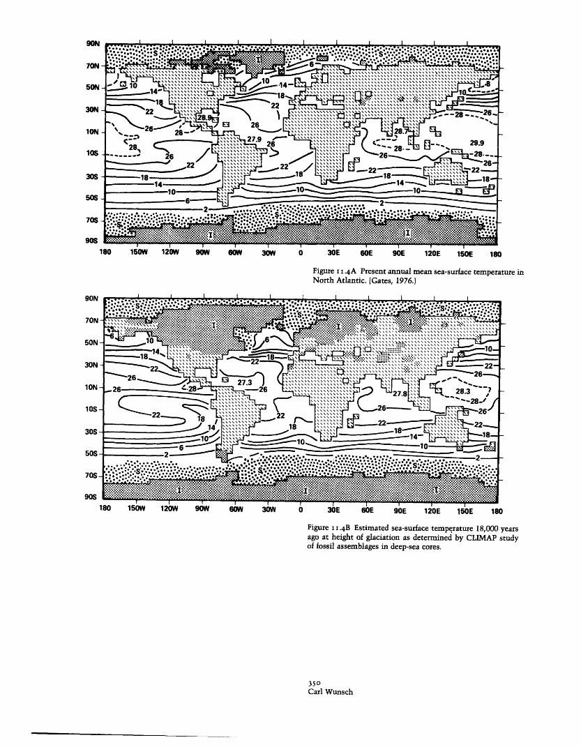
Figure I .4A Present annual mean sea-surface temperature inNorth Atlantic. (Gates, 1976.)
Figure i .4B Estimated sea-surface temperature 18,000 yearsago at height of glaciation as determined by CLIMAP studyof fossil assemblages in deep-sea cores.
350Carl Wunsch

minor climatic fluctuations may be fruitless. Thechanges 18,000 years ago could have been much greaterat depth than at the surface; whether this is indeedtrue is now the subject of study.
The success of oceanographers in obtaining at leastqualitative descriptions of the large-scale circulationby combining observations made many years, or evendecades, apart in time is, as noted, a reflection of someunderlying truth about the frequency-wavenumbercontent of the baroclinic variability in the ocean. Themost intense fluctuations seem to occur on a spatialscale small compared to the large-scale mean gyres. Onthe other hand, if one is to seek the role of the oceanin climatic changes, it is likely to be reflected in verylarge-scale low-frequency oceanic fluctuations, on theintuitive assumption that perturbations to the atmos-phere owing to small-scale fluctuations of the oceanwill tend to be "integrated out" by the atmosphere. Ina nonlinear system like the atmosphere, the validity ofthis assumption is by no means obvious, but it is areasonable initial hypothesis. One can then attempt tosearch for very large-scale changes in ocean circulationon time scales of years and space scales of thousandsof kilometers.
For a number of reasons, most of the work on thishypothesis has been conducted in the Pacific Ocean.First, it has long been hypothesized (Bjerknes, 1969,Namias, 1972) that the U.S. continental weather maybe sensibly modified by large-scale thermal anomaliesover the Pacific Ocean. Bjerknes provided some specifichypotheses now generally called "teleconnections."Beginning in the early 1960s investigators at theScripps Institution of Oceanography began a series ofinvestigations to attempt to define, and ultimately tounderstand, both the apparent anomalies themselvesand the role they might play in U.S. climate andweather. It seems clear that the anomalies are real; butit also seems fair to state at many of the links betweenthe anomalies and weather are the result of wishfulthinking rather than evidence (e.g., Davis. 1976, 1978a).
Sea Level Few extended time series for studying verylong-period motions are available; the only real dataconsists of sea-level measurements. The idea of usingtide-gauge records for studying fluctuations of geo-strophically balanced currents evidently dates back toSandstrom (1903), although Montgomery (1938b)seems to have been the first to actually attempt it.
The spectra presented here in figure 11.5 (see alsofigure 11.9), in Wyrtki (1979), in Munk and Cartwright(1966) and in other places, of the longest available rec-ords [circa 100 years-the longest record may be theone from Brest analyzed by Cartwright (1972), whichruns from 1856 to date] are red, although decreasinglyso beyond periods of 1 year (see Figure 11.9).
The limits of this increasing power with decreasingfrequency are unknown. In some regions, one may beseeing slight fluctuations in the geodetic levels of thetidal gauges; in other regions this seems implausible.Taken at face value, the red spectra suggest that thereindeed may be barotropic, large-scale fluctuations ofthe oceanic gyres. One infers that they are barotropicbecause of the decrease in temperature variance withlengthening period appearing in the temperature spec-tra (see section 11.2.4), and large scale because of thedecreasing variance in the moored-current spectra atlong periods. But the evidence is ambiguous.
A number of attempts to understand the physics oflong-period fluctuations in sea-level records have beenmade (Wunsch, 1972c, Groves and Hannan, 1968;Groves and Zetler, 1964; Shaw and Donn, 1964;Schroeder and Stommel, 1969). The major difficulty isthat not only are long records few, but the number oflong simultaneous records, which are vital for under-standing spatial correlations and possible propagation,are even rarer.
Sea-level fluctuations at a point are a complex sum-mation of many different physical phenomena. Muchof the work cited above was dedicated to attemptingto unravel the role of local weather variables in sea-level fluctuations. In the open sea, using island data,Groves and Hannan (1968), Wunsch (1972c), and othersfound an inverted barometer response at periods longerthan about a day. At periods of months and longer, theeffects of wind tend to dominate. The procedure fordeducing the relative role of the two wind componentsand pressure is not straightforward because the weathervariables are themselves coherent; a multiple regres-sion procedure described in the cited papers is required.With localized weather effects removed one can thenask whether fluctuations from location to location arecoherent and can be ascribable to any particular knownphysics. A major problem has been (e.g., Groves andHannan, 1968) the absence of measurable coherencesbetween the few simultaneous island records available.The entire procedure is made very difficult because theprior removal of the fluctuations coherent with localweather may remove global phenomena that are forcedby the meteorology.
The clearest picture of large-scale fluctuations of sealevel stems from the work of Wyrtki (1974, 1975a) inthe Pacific. Previous work in the Atlantic by Schroederand Stommel (1969) and Wunsch (1972c) had suggestedthat on the time scale of months that sea level was toa large extent responding to fluctuations in dynamicheight relative to reference levels at about 1500 db(decibars). Wyrtki (1979) has shown in the tropical andequatorial Pacific Ocean that he could find large-scalecoherent patterns of dynamic height variation that also
35ILow-Frequency Variability of the Sea

,.5IO0
103
102I01
100
10
CO
GLAND
B
103
A 102
CU0
101
100
-3 I2
10- 3 10- 2 10- I
FREQUENCY (cpd)10o 10- 3
A - AZORESB --- HILO, HAWAII
-2
A
B- \\
10-2 10-IFREQUENCY (cpd)
100
Figure II .5 A Spectra from a few representative sea-level rec-ords (log-log form).
ItI
I
/I
A - BALBOAB --- SAN FRANCISCOC -x-- BERMUDAD --- NEWLYN, ENGLAND
A.
I. b
1.4
1.2
1.0
z
W 0.8ir'I-aQ
0.6
0.4
0.2
0.0o10- 3
10-2 lo0- 100FREQUENCY (cpd)
Figure I i.5 B Spectra from sea-level records in an energy- (var-iance-) conserving form; notice that units are arbitrary--onlyrelative spectral shapes are comparable. Canton I spectrum
10-3
A - AZORESB --- HILO, HAWAIIC --- CANTON,I
10-2 i0-1FREQUENCY (cpd)
I00
contains sharp peaks at 4 and 5 days, described by Wunschand Gill (1976). The fortnightly tide is also apparent in thespectrum.
352Carl Wunsch
zw
J EW o
J
U)
1.6
1.4
1.2
1.0
.-
I 0.8
0.6
0.4
0.2
on
· ·
J
- -- -···-------
lu- r. A _
rA l/ AA r
104-
_
_ _
16-_
rr
_
IA
I
_
_
_
_
__
_ _
v _

shows up convincingly in the Pacific tide gauges. Hehas been able to relate his observations to fluctuationsof the large-scale tropical current systems of the Pa-cific. Much of this work has been directed toward un-derstanding of the relationship between the ocean fluc-tuations and the catastrophic economic and climaticeffects of the E1l Nifio phenomenon (see chapter 6).
There does seem to be a link (or at least a correlation)between trans-Pacific sea-level fluctuations, the occur-rence of warm water on the coast of Peru, and grosschanges in the wind field over the Pacific. These latterchanges are supposed to be part of the so-called south-ern oscillation and the Walker cell circulation(Bjerknes, 1969) in the atmosphere. Thus there is someindication of an actual coupling of large-scale oceanicand atmospheric fluctuations, but the global extent ofthe phenomenon and the causal links are very obscure.The data base is inadequate to be truly definitive, butthe apparent patterns are plausible and are a highlypromising line for future research into gyre-wide fluc-tuations, at least in the near-equatorial oceans.
For the purely oceanic phenomenon one needs ulti-mately to understand the extent to which one is seeingdynamic topography variations relative to a fixed ref-erence level (a difficult idea to rationalize) or fluctua-tions possibly representable as vertical normal modes.In this latter case, the changes in sea-surface topogra-phy imply equivalent deep-water fluctuations, whichare, however, at this time totally unknown.
Presumably similar fluctuations occur in the Atlan-tic and Indian Oceans. But the absence of many islandsin these oceans has largely precluded the determination
EO
F-toUr
of sea-level fluctuations there. The Azores and Ber-muda records were examined by Wunsch (1972c) andthe Iceland record by Donn, Patullo, and Shaw (1964).Most of the low-frequency variability of the IndianOcean, especially in the western portions, is obscuredby the very large monsoonal signals.
Thermal Record The most conspicuous low-frequencyphenomenon in the ocean is the sea-surface tempera-ture anomalies of the Pacific that have been studiedintensively the past two decades. Barnett (1978) hasreviewed this work. A primary motive for the interestwas the Bjerknes (1969) teleconnection hypothesis.There is little doubt that extensive changes in sea-surface temperature do exist and can persist for monthsand years. Figure 11.6, taken from Barnett (1978), is amultiple-year record of temperature (fluctuations aboutthe long-term mean) at Talara, Peru, and ChristmasIsland. These "anomalous" temperatures occupy majorareas of the Pacific Ocean. Figure 11.7 displays the firstthree empirical normal modes of Pacific sea-surfacetemperature (from Barnett and Davis, 1975). Thesemodes describe slightly under half the total variance ofthe Pacific sea-surface temperature fluctuations; theirimmense scale is apparent.
Much of the interest in the anomalies has been inthe possibility that in changing the lower boundarycondition of the atmosphere, fluctuations in the at-mosphere might be induced on the long oceanic timescale rather than on the intrinsically short atmospherictime scale. Studies of the question have been hampered
Year
Figure i I.6 Sea-surface temperature anomalies at Talara, Peru(upper) and at Christmas Island (lower). (Barnett, 1978.)
353Low-Frequency Variability of the Sea

Figure I I.7 Three lowest empirical normal modes of sea-sur-face temperature anomaly field in North Pacific Ocean. No-tice very large scales involved. (Barnett and Davis, 1975.)
354Carl Wunsch
__1_ 1___�

by the inherent noisiness of the atmosphere. But Davis(1976) showed that changes in the ocean tended to lagthose in the atmosphere, thus implying that the anom-alies were being driven by the atmosphere rather thanthe reverse. In a later paper, Davis (1978a) obtainedsome atmospheric predictability from sea-surface tem-perature anomalies stratified by season. But the samepredictability was found using atmospheric sea-surfacepressure anomalies. The cause-and-effect relationshipsthus remain unknown. Rowntree (1972) and Kutzbach,Chervin, and Houghton (1977) have studied the reac-tion of the atmosphere to imposed sea-surface temper-ature anomalies. With unrealistically large anomalousvalues, an atmospheric reaction can be detected, butits significance is still not understood.
Frankignoul and Hasselmann 1977) have shown thatpurely random forcing of the ocean by the atmospherecan plausibly generate anomalies. The degree to whichthe surface features represent anomalies of heat con-tent, that is, represent subsurface features as well, alsois not clear. White and Walker (1974) have displayedtime-depth diagrums for temperature anomaly at threepositions in the Pacific Ocean (figure 11.8). Gill (1975b)shows similar data and perhaps the simplest conclu-sion to be drawn is that the physics governing sea-surface temperature anomalies is a combination of in-teraction with the atmosphere and with deeper oceandynamics in a form that varies in space and time. It isdifficult to relate the gyre scale fluctuations describedby Wyrtki, to the anomalies, except in the case of ElNifio.
Observations in the Atlantic similar to those madein the Pacific have been described by Rodewald (1972).On a much longer time scale, there are variations inthe extent of the pack ice in the vicinity of Icelandthat seem relatable to atmospheric changes. Oceanicchanges that may accompany the atmospheric fluctua-tions beyond those locally involved with the sea iceare unknown.
The significance and meaning of apparent large-scalegyre-wide fluctuations is obscure. Attempts at dem-onstrating massive fluctuations in western boundarycurrent flows that might be of real climatic significancehave generally not been convincing. The wild variabil-ity in estimates of the volume transport of the GulfStream north of Cape Hatteras (see Worthington, 1976)has generally been due to varying methods of estimat-ing reference levels, and there are no convincing dem-onstrations of nonseasonal volume-transport fluctua-tions. Similar remarks apply to the AntarcticCircumpolar Current, where 100% changes in esti-mates of the volume transport essentially disappearwhen appropriate reference levels are used (Nowlin,Whitworth, and Pillsbury, 1977).
Much of the problem of documenting real low-fre-quency large-scale fluctuations in the major oceangyres may be looked upon as a classical problem ofaliasing. Momentary fluctuations in the mass field,which owe their existence to short-period time varia-bility, may inappropriately be interpreted as represent-ing much lower-frequency phenomena (Worthington,1977b). The large-scale baroclinic structure of the oceanis remarkably stable and one cannot store largeamounts of water anywhere in the system withoutraising havoc with sea level. Real low-frequencyoceanic changes on large scales appear to be subtle anddifficult to detect in the presence of the much strongershort-period fluctuations discussed below in section11.2.4.
11.2.3 Annual VariabilityThe entire atmosphere-ocean system is subject to alarge thermal forcing with an annual period as the sunmigrates meridionially throughout the year. In the at-mosphere the seasonal change in character is of courseenormous at mid- and high-latitudes. The ocean wouldrespond both to the direct thermal forcing of the sunand to the indirect thermal forcing due to the changein air-sea temperature difference. One anticipates,from calculations like those of Gill and Niiler (1973)and Frankignoul and Muiller (1979), that except in themixed layer and on the equator the response to bothwould be quite small. Even in the region of intensewintertime air-sea heat exchange that occurs in thenorthwest regions of the northern hemispheric sub-tropical gyres and that leads to the formation of 18°Cwater in the Atlantic and 16°C water in the Pacific, theoceanic response seems localized and nearly passive(Warren, 1972; Worthington, 1959). More generally Gilland Niiler (1973) show that the heat budget is essen-tially locally controlled with lateral advection compar-atively unimportant. Only the upper 100-200 m ofocean is involved.
It is the oceanic response to the annual cycle in thewind field that is likely to dominate the annual period.The annual line in the wind field at the ocean surfaceis superimposed upon a background continuum, and issurprisingly weak (figure 11.9) even in the monsoonregions of the Indian Ocean. The annual line at mid-latitudes, e.g., at the location of Bermuda, seems tocarry no more than about 1% of the total wind-fieldvariance in periods between 10 years and 1 day.
Patullo, Munk, Revelle, and Strong (1955) analyzedthe available tide-gauge records for the annual varia-bility in sea level and provide an interesting globalmap. Most of the inverted barometer-corrected sea-level signal between 40°N and 40°S is in "steric"height, i.e., the essentially passive change resultingfrom the warming or cooling of the upper water col-
355Low-Frequency Variability of the Sea

1950 1951 1952 1953 1954 1955 1956 1957 1958 1959 1960 1961 1962 1963 1964 1965 1966 1967 1968 1969
DMJ SDUJ SDMJSDJ SDMJSDMJ S DMJSDMSMSDM SMSDM SDMJ SM JSDMJS DMJ SDMJ SDMJS D
Figure I .8 Time-depth diagram of subsurface anomalies oftemperature at ocean station N (upper at 30°N, 140°W) and atstation V (lower at 34°N, 164°E). (White and Walker, 1974.)
356Carl Wunsch
i~~ ~ ~ ~ ~ ~ ~~~~~~~~~~~~~~~~~~~~~~~~~~~~~~~~~~~~~~~~~ I -_

umn. The International Geophysical Year (IGY) datawere subsequently examined by Donn, Patullo, andShaw (1964), resulting in much the same conclusions.The effects of the direct steric changes do not appearto be visible below about 300 m in subtropical latitudes(Wunsch, 1972c).
The change in elevation of the sea surface owing tothese direct heating effects should give rise to a weakannual surface circulation; this circulation would beweak because of the very large scale over which thesteric effects are induced.
In their analysis of the annual variability, Gill andNiiler (1973) concluded that over most of the oceanthe major baroclinic effects of the wind would be toinduce an Ekman suction at the annual period with aconsequent response of the main thermocline. Thissignal seems to be lost in the background movementof the thermocline in response to other forces. By andlarge, deep current meter or temperature records of afew years duration do not display any recognizable an-nual variability above the continuum [although White(1977) claims he sees annual-period baroclinic Rossbywaves generated at the eastern boundary of the Pacific].
The western boundary currents do show some formof annual cycle; in the Florida Current the cycle man-ifests itself over the entire water column from top tobottom and has been convincingly documented by Ni-iler and Richardson (1973) as an essentially barotropicchange. Farther north, Fuglister (1947, 1951) docu-mented a cycle in the surface temperatures and flowby using ship-drift reports. The extent to which thisannual cycle penetrates into the deep water north ofthe Florida Straits is unknown. Much earlier, Iselin(1940a) had attempted to study the annual cycle of theGulf Stream between Woods Hole and Bermuda. Overa 3-year period, he found transport fluctuations be-tween 76 and 93 x 106 m3 -1, with the system strongestin summer. In view of the problems of aliasing referredto above, the necessity for a fixed reference level, andthe short record duration, it is difficult to assess thesignificance of this result.. Wyrtki (1974) has shown anannual cycle in the surface circulation of the equatorialPacific in response to the annual trade-wind changes.Elsewhere (Wyrtki, 1975a) he finds little annual signalexcept in the immediate vicinity of the Kuroshio.
There is a fundamental problem in using the annualcycle to understand the dynamics of the ocean. Becausevirtually all physical variables (wind, temperature, sealevel, etc.) show an annual line, it is difficult to sortout cause and effect. Narrow-band processes tend tocontain much less useful information than randombroad-band ones.
I YEAR
I-z
arLn-0
QNZ ',,
E
zo0n,
i
106
10- 4
A BERMUDAR ---- CANTON I
V
i0- 3 10-2
FREQUENCY (cpd)10-I
Figure I .9A Spectra of wind records (displayed in figure 11.2but at much higher resolution), showing the annual peak.
U-CAz
0 0U
wCLUUJII
W
U)
103
100
,LBOANFRAN CISCO-RMUDAW LYNN TON
I
\I
E
10 10FREQUENCY (c
I2 -2 i010
:pd )
Figure II. 9B Spectra of long sea-level records (displayed infigure 11.5 but at much higher resolution), showing resolvedannual peak.
11.2.4 The MesoscaleThe ocean appears to be in a turbulent state with avery high Reynolds number, and as that fact has come
357Low-Frequency Variability of the Sea
107
_
10 5_
10 4 _._
or-2
_
101
_10- 4
to be more widely appreciated attention has shiftedfrom the very large-scale mean flows and large-scalevariability discussed above, to the nature of the tur-bulence itself. Much of this shift in focus has comeabout because of technical innovations. These madepossible multimonth in situ time series independentof ship endurance limitations. The presence of disturb-ances of spatial scales of 0(100 km) is obvious in con-ventional hydrographic sections (figure 3b from Fuglis-ter, 1960) but studies of these undulations in the iso-pyncnals were impossible before about 1970. In dis-cussing the mesoscale, we include all fluctuations withthe appropriate space and time scales, including con-tinental shelf waves even though these latter motionsare essentially nonturbulent in character.
Shelf Waves These waves were discovered by Hamon(1962), who found that sea-level fluctuations on theeast coast of Australia were not in isostatic balancewith atmospheric pressure (i.e., the inverted barometereffect failed to apply). Robinson (1964) pointed out thatHamon's results could be rationalized in terms of top-ographic Rossby waves excited by atmospheric pres-sure forces [the basic physics of the phenomenon isdiscussed by Lamb (1932, §212)]. Subsequently Adamsand Buchwald (1969) demonstrated that wind stresswas a much more efficient driving mechanism andobtained reasonable agreement between theory and ob-servation.
Since the original observations of Hamon and thelater theoretical work much attention has been paid tothese waves for a number of reasons. Unlike mostopen-ocean variability, linear theory seems to applyreasonably accurately, the shallow water of the conti-nental shelves is comparatively easily accessible, con-ventional harbor tide gauges can often be used, and thewaves presumably play a major role in the time-de-pendent response of the low-frequency shelf circulationto external forces.
We shall not dwell on the subject here because anumber of comprehensive reviews have appeared re-cently (e.g., LeBlond and Mysak, 1977; Munk, Snod-grass, and Wimbush, 1970; Mysak, 1980; and see chap-ter 10). The detailed connection between open-oceanvariability and shelf waves is unknown. It is possible,however, that, in some situations, the waves generateopen-ocean effects rather than merely being the re-sponse to local winds or forcing from the open sea. Anexample of this may be in the Gulf Stream System(Diing, Mooers, and Lee, 1977; Wunsch and Wimbush,1977), where waves of several days period are observedin the Florida Current region. A number of authorshave suggested that these waves may trigger meandersand other motions of the Gulf Stream System in theregion north and east of Cape Hatteras. No actual cause
and effect has ever been demonstrated; the topic isdiscussed in chapter 4.
Gill and Clarke (1974) made plausible the hypothesisthat shelf waves (they specifically emphasized the bar-oclinic Kelvin wave) play a fundamental role in thespecial subclass of mesoscale variability called coastalupwelling. If this is correct (and it permits remote forc-ing to give rise to strong localized effects) there can bea dramatic influence of shelf waves on local climatol-ogy. In some cases (e.g., the E1l Nifio phenomenon),coastal upwelling may be part of an ocean-wide, andperhaps even global, system involving both the oceanand atmosphere. The extent to which such events link-ing shelf waves (which may be thought of as a localfocusing and amplification of comparatively weak forc-ing) are part of a global system is the subject of muchwork at the present time. That such links exist seemsclear; their extent is obscure. Upwelling deserves aspecial discussion of its own; the reader is referred toO'Brien et al. (1977).
In our more general context, shelf waves provide asimple (i.e., nearly linear) example of mesoscale vari-ability that in some cases exhibits the combined effectof rotation, topography, and baroclinicity. The litera-ture contains a large number of special cases of topog-raphy for which analytical solutions are available. Thebasic physical phenomena are Kelvin waves trappedagainst the coast, double Kelvin waves at the shelf edge(Longuet-Higgins, 1968c), barotropic topographicRossby waves (Rhines, 1969a), and baroclinic topo-graphic Rossby waves (Rhines, 1970). In the presenceof stratification finite bottom slopes couple the differ-ent wave types together and one is generally driven tonumerical solutions (Wang and Mooers, 1976), but theunderlying physics may be understood from the sim-pler physical situations. Ou (1979) has significantlyadvanced the analytic treatment of the problem. Hen-dershott in chapter 10 discusses these topics further.
Very similar effects occur at mid-ocean islands (Lon-guet-Higgins, 1969b; Wunsch, 1972b; Hogg, 1980);both barotropic and baroclinic trapped waves can occurand particular bottom-slope configurations can modifyqualitatively the dispersion relations. The barotropiccase with varying topography had been treated by Lamb(1932, §212), for the inside of a cylinder, rather thanfor the outside, as is appropriate to the oceanic case(the mathematical differences are slight).
Mesoscale Eddies Much of what we now call themesoscale variability, or the eddy field, is plainly whatearly investigators like Maury had in mind when theydescribed their difficulties with time-dependent mo-tion. In a modem context, these motions were firstquantitatively measured in 1959 (Crease, 1962; Swal-low, 1971) in a noteworthy experiment. Using the
358Carl Wunsch
_I_ _ _ e � _ _ __ � �__

newly developed neutrally buoyant floats (Swallow,1955) they detected motions west of Bermuda withvelocities of up to 40 cm s-1 and apparent time scales ofroughly 40 days. Their measurements were analyzedin an important paper by N. A. Phillips (1966bl, whosuggested that they could be treated as a sum of linearRossby waves driven by the wind. Phillips's modelcould not reproduce the high velocities (but see Har-rison, 1979a). Later, Rhines (1971b) suggested that theywere intensified by bottom trapping on the BermudaRise, but this too seems inadequate.
By 1970, the combination of the knowledge of theexistence (at least in the area studied by Swallow andCrease) of very intense time-dependent motions, of thetheoretical work on turbulent interaction, and of themeteorological picture alluded to, led to a series ofexperiments aimed at elucidating the nature of themesoscale in the ocean [Koshlyakov and Monin (1978)discuss the history of parallel Soviet efforts, whichseemingly had a very different intellectual content]. Itseems fair to call the 1970s the "decade of the meso-scale" in physical oceanography both for the intensiveefforts that went into it and for the striking advancesin knowledge that occurred. The initial tentative ob-servational programs (e.g., Gould, Schmitz, andWunsch, 1974) had first to convince the investigatorsof the reality of the phenomenon; it was only then thatserious efforts could be mounted to understand meso-scale physics. Although 100-day time-scale fluctua-tions are much more humanly accessible than the in-terannual frequencies described above, it is stillimportant to note that to obtain 20 degrees of freedomat a resolved 100-day period for a spectrum of velocity(or anything else) from a point measurement requires1000 days of data. Thus studies of the mesoscale arenecessarily in their infancy.
It is probably a mistake to overemphasize the me-soscale as an isolated phenomenon. There is reason tobelieve that the very large-scale phenomena describedpreviously and the mesoscale are to a great extent sim-ply manifestations of the extremes of a continuum.Ocean variability occupies a broad space-time spec-trum; for purely experimental reasons it has been con-venient to study the 100-km scale separately from the5000-km scale. But in the long term, it will be neces-sary to understand their linkages.
On the other hand, there does appear to be a "bulge"or plateauing of low-frequency spectral variability inthe very roughly defined period range of 50-150 days.It is apparent even in the sea-level spectra, and asnearly as one can tell this plateau is a global phenom-enon. We shall follow Richman, Wunsch, and Hogg(1977) in calling this the eddy-containing band. At thelow-frequency end this band fuzzily merges into theannual and interannual variability. We shall refer to
frequencies above the eddy-containing band as the iso-tropic band because of the energy isotropy there. Forthe moment this distinction into separate bands is kin-ematically descriptive; there may also be a dynamicdistinction.
Much of the work on mesoscale variability wasfocussed in the Mid-Ocean Dynamics Experiment(MODE-1) which ran from about 1971 to 1973. Manyof the results have been summarized elsewhere (MODEGroup, 1978; Mode-1 Atlas Group, 1977; Richman,Wunsch, and Hogg, 1977). The effort was continued inPOLYMODE-as an amalgam of the early Soviet ef-forts Polygons (Brekhovskikh, et al., 1971) and theMODE experiment. By the time of POLYMODE, how-ever, the mesoscale field was widely recognized as auniversal, important phenomenon and was being stud-ied as part of many aspects of oceanography, includingthe biological ones.
The detailed results of these experiments are tooextensive to be described here, and, indeed, their fullimplications are not understood. But it appears that aneddylike field of variability is nearly universal in theocean (MODE Group, 1978; Schmitz, 1976, 1978; Bry-den, 1979; Bernstein and White, 1974, 1977; Hunkins,1974) and is normally much more energetic than thelocal mean flow (see figure 11.10).
The time variability of the North Atlantic ocean onthe large scale is represented by figure 11.11, takenfrom Dantzler (1977) [see Bernstein and White (1977)for a similar discussion of the North Pacific and Lutje-harms and Baker (1979) for the Southern Ocean]. It isa compilation of the temperature variance in the NorthAtlantic from expendable bathythermograph (XBT)measurements. The variance of temperature, whichmay be thought of as a crude measure of potentialenergy of the fluctuation field, shows a large-scale mid-ocean trough, with steep gradients toward the bound-aries, and especially toward the Gulf Stream System.This figure, while extremely suggestive, also illustratesseveral of the caveats that must be applied to discus-sions of the field of variability.
The variability field is commonly referred to as theeddy problem; the implication is that eddies have anidentifiable scale, nearly unit aspect ratios and possiblyeven closed streamlines. But figure 11.11 is simply arepresentation of the time variability of the North At-lantic irrespective of its source. For example, it is wellknown that the Gulf Stream moves and meanders (Fug-lister, 1963; and see chapter 4). Such variability willappear in figure 11.11 and presumably represents muchof the energy appearing in the northwest region. Thelarge-scale, low-frequency variability described in theprevious sections would also be included but probablyis only a small fraction of the variance. It is more thana semantic distinction to wish to distinguish the var-iability of migrating jets from that of features with
359Low-Frequency Variability of the Sea

Figure II.IoA Five-degree-average chart, based upon ship-drift reports of mean surface kinetic energy. (Wyrtki, Magaard,and Huyer, 1976.)
90E 1200 1500E 1800 1500W 1200 90° 600 30°W 00 300E 600 90o 1100
Figure I i .ioB Five-degree-average chart, based upon ship-driftreports of total fluctuation kinetic energy (Wyrtki, Magaard,and Hager, 1976). Superimposed upon the chart are kineticenergy densities (cm2 s-
2 cpd-) from moored current meters,at a 50-day period at nominal depths of 500 m and 400 m.Actual depths are shown.
360Carl Wunsch
600N
500
40°
30 °
200
I 00
200200
40
500
60S
I

80 0" d o40o
I: I : I* ;..;r
1.
RN 'ilf WQrI
10*ir rCs,-,
K
-' - ' -J-I1--J ?-I
'!
I
I
· I / I __.- IEOIKLJ_ .IL
5571-5791-6001 1
30 ¢ I
15Cc m-
. I
30 Cms-l
55710-5796-6 Q6
30 88 8
5671 -5801600 m
30 em'1
5673-5803-612510oo m
30 5cms'l ' / ,-
5674-5804-6126IS00 m
30 cs-l 470
5675-5805-6129ooo00 m
30 Cm sl
ESRODAY 1975-1977
(11.12A)
Figure II.I2A,B Three-day average-velocity vectors from twolocations (35°56'N, 55°06'W and 31°36'N, 55°05'W), respec-tively, in the North Atlantic (see figure 11.11B). Note large
120ioE 22R 3Y 1975 -977TERRDRY 1975-1977
(1 1.12B)
change in energy level over comparatively small separation inposition between the two moorings. The difficulty of defininga mean flow from such measurements should be obvious.
5571-5791 -6001
0 .3 ] - . .. 3
5573-5793-6003
1.-O m |-A
5575-5794-600u,
500 8 ] 3.
55710-5796-60062.2
5671-5801
600 m
]::
5673-5803-6125a.
tooo m
5674-5804-6126s. I
soo m
]
5675-5805-6129.s
ooo m
.~
o0 2o0 320 ss s5 2ss 355s s 9gYERDORA 1975-1977
(11.12C)
020 2k0 320 5 Iss 25s 3s5s 8T ldTERDORI 1975-1977
(11.12D)
Figure II.I2C,D Temperature records from same mooringsas in figures 11.12A and 11.12B. Note change in character andamplitudes of fluctuations.
362Carl Wunsch
3,s5 33 l3
'117~pC
_ · · r · -T---- -T--- r
-a~~~~ n-r/r - II CC 7CC 7011
"-1/"�G·"
*uwrs�n�-�i�wV-·--�
are the velocity vectors and temperature measure-ments (averaged over 24 hours) from two moorings inthe north Atlantic at positions 35°56'N, 55°06'W and31°36'N, 55°05'W. One sees a very complex and ener-getic time variability over the record lengths (nearly 27months in the longest records), a considerable resem-blance between different levels in the vertical, and avery marked decline in energy levels over the 400-kmseparation between the moorings. This remarkablechange in energies is roughly consistent with that im-plied by figure 11.11, although the change is muchsteeper because of the 5° averages in figure 11.10.
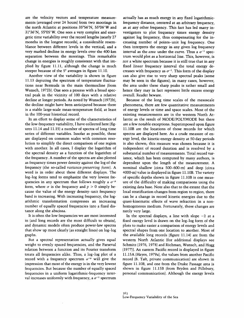
Another view of the variability is shown in figure11.13 depicting the spectrum of temperature fluctua-tions near Bermuda in the main thermocline (fromWunsch, 1972b). One sees a process with a broad spec-tral peak in the vicinity of 100 days with a relativedecline at longer periods. As noted by Wunsch (1972b),the decline might have been anticipated because thereis a stable large-scale mean-temperature field, at leastin the 100-year historical record.
In an effort to display some of the characteristics ofthe low-frequency variability, I have collected here (fig-ures 11.14 and 11.15) a number of spectra of long timeseries of different variables. Insofar as possible, theseare displayed on common scales with common reso-lution to simplify the direct comparison of one regionwith another. In all cases, I display the logarithm ofthe spectral density as a function of the logarithm ofthe frequency. A number of the spectra are also plottedas frequency times power density against the log of thefrequency (the so-called variance-preserving form). Aword is in order about these different displays. Thelog-log forms tend to emphasize the very lowest fre-quencies in any spectrum that follows roughly a r-pform, where r is the frequency and p > 0 simply be-cause the value of the energy density-unit frequencyband is increasing. With increasing frequency, the log-arithmic transformation compresses an increasingnumber of equally spaced frequencies into a fixed dis-tance along the abscissa.
It is often the low frequencies we are most interestedin (and long records are the most difficult to obtain),and dynamic models often produce power-law spectrathat show up most clearly (as straight lines) on log-loggraphs.
But a spectral representation actually gives equalweight to evenly spaced frequencies, and the Parsevalrelation between a function and its Fourier transformtreats all frequencies alike. Thus, a log-log plot of arecord with a frequency spectrum r- p will give theimpression that most of the energy is in the very lowestfrequencies. But because the number of equally spacedfrequencies in a uniform logarithmic-frequency inter-val increases uniformly with frequency, a (r- ' spectrum
actually has as much energy in any fixed logarithmic-frequency distance, centered at an arbitrary frequency,as at any other frequency. This fact has led many in-vestigators to plot frequency times energy densityagainst log frequency, thus compensating for the in-creasing number of points-unit log frequency. Onethen interprets the energy in any given log frequencyinterval as the area under the curve. Thus a a-' spec-trum would plot as a horizontal line. This, however, isnot a white spectrum because it is still true that in anyfixed linear frequency interval the total energy de-creases with frequency as (r-. This form of the displaycan also give rise to very sharp spectral peaks (somemay be seen in the figures); in many cases, however,the area under these sharp peaks is rather small andhence they may in fact represent little excess energyoverall. Reader beware.
Because of the long time scales of the mesoscalephenomena, there are few quantitative measurementsof energy levels or time and space scales. Most of theexisting measurements are in the western North At-lantic as the result of MODE/POLYMODE but thereare a few notable exceptions. Superimposed upon figure11.10B are the locations of those records for whichspectra are displayed here. As a crude measure of en-ergy level, the kinetic-energy density at 50-day periodsis also shown; this measure was chosen because it isindependent of record duration and is resolved by asubstantial number of measurements. Total record var-iance, which has been computed by many authors, isdependent upon the length of the measurement. Anominal shallow (circa 500-600-m) and deep (circa4000-m) value is displayed in figure 11.10OB. The varietyof specific depths shown in figure 11.10OB is one meas-ure of the difficulty of making comparisons using theexisting data base. Note also that to the extent that thelocal stratification changes from region to region, therecan be a change in record kinetic energies due to thequasi-kinematic effects of wave refraction in a non-homogeneous medium. Fortunately, these changes arerarely very large.
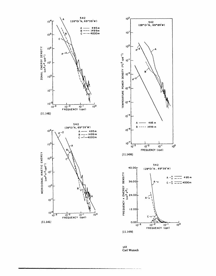
In the spectral displays, a line with slope -2 at afixed energy level is drawn on the log-log form of theplots to make easier a comparison of energy levels andspectral shapes from one location to another. Most ofthe available long records (figure 11.14) are from thewestern North Atlantic [for additional displays seeSchmitz (1976, 1978) and Richman, Wunsch, and Hogg(1977)]. An eastern Pacific record is displayed in figure11.15A (Hayes, 1979a), the values from another Pacificrecord (B. Taft, private communication) are shown infigure 11.10OB, and one from the Drake Passage area isshown in figure 11.15B (from Bryden and Pillsbury,personal communication). Although the energy levels
363Low-Frequency Variability of the Sea

17.000 HOURSIQ.0 3000 1000 48 21 12I I I I
--.28
N f -4.27
\t{\
I I I
103
102
70
101'
Ioo-. I
U . 10
,, -2Z 1040
ia
· PANULIRUS (WUNS10-5- -- + BOTTOM CABLE (H
STOMMEL,8 MUNKo CABLE (WUNSCH 8
Figure II.13 Spectrum of temperature at Bermuda in themain thermocline from record duration of 13 years. (A) is log-log form, (B) variance-preserving form. Bulk of energy isaround 100-day periods. (Wunsch, 1972b.)
i.
10-7
10-5 10-4
++° t f-l.6 5
d+%
f- 35
SCH. 1972) °\AURWITZ. o\
1959)a DAHLEN. 1970) ,,
0P
I I I f IIiI I I I I I103
10-2
0-FREQUENCY (cph)
100 10l 102
(1 1.13A)
DAYS756 200 42
10- 5 10-3 10-2FREQUENCY (cph)
(11. 13B)
364Carl Wunsch
2MINUTES
1 87
I I
-i
I
HOURS20 12.42
2.C
1.0v
0
0
I I I I I
0
00 * .
· _ .60 +
i _I I 1 I I I + I +I i , , h+ + 't+ ++ + t +t +'
i0-1 100
~~~~~
I
104
_
I
I

557- 579-600(35°56'N, 55006'W)
-A
10-2 10- 1FREQUENCY (cpd)
A --- 600mB --- 100OmC --- 1500mD -4001 m
z
cr
W -
ZNW E
z 03rWI
In
o00
.A10'
103
10 I
10(
10-1
10-3
557 - 579 -600(35056'N, 55006'W)
-x- 600 m--- 100Om---- 1500m
4001 m
C
O'
I I10-2 10 - 10
FREQUENCY (cpd)
(11. 14B)
Figure I.I4 Spectra of velocity and temperature from a va-riety of positions in the western North Atlantic, log-log formsare always shown. In a number of cases, the variance-preserv-ing plots are also displayed. On log-log forms a straight lineof slope 2 and fixed energy level is shown for comparisonpurposes. Variance-preserving plots for temperature are on anarbitrary scale because large range of values defeats a linear-scale display.
zI-
Z W E
z
c2
l.WU-.r"I.U I
12.00
0.00I
5 57-579 -600
ridional 600mridional 1000 mridional 1500mridiona 14001 mial 4001 m
0
FREQUENCY (cpd)
(11.14C)
365Low-Frequency Variability of the Sea
I-
zW -
Z NE
0N
10'
00
I10~
(11.14A)
I I
I104 -
103
02
-
[-
i0- L !I10-3

557- 579 -600(35056'N ,55°06'W)
1.0
x-- 600 m--- 1000m
---- 1500m-4001 m
U)zWo 0.8
z U
W 0.6f z
0.4
x
Uz 0.2W
0.0
557- 579 -600( 35°56'N, 55°06'W)
600m000 m
)0
FREQUENCY (cpd)(11. 14E)
10-2 10-1FREQUENCY (cpd)
I-U)zW --o
U
W iZ 0w E
z0N
10- 3 10- 2 10- FREQUENCY (cpd)
(11.14F)
366Carl Wunsch
I0
I01
0 - I
n-zW0
Z
NW
-Ila:L,.
10-6
I I I
(11.14D)
1oo
- 628 m- 1028 m-4030 m
--
!-
10
10 4
I0!

628m1028m1030m
c,zUL0
0
Z bJ u
n o
2Dp-Ln
a
FREQUENCY (cpd)
628 m
1028m
4030m
567- 580-612( 31° 36 'N, 55°05'W)
n
\
\ \B A
\ I
FREQUENCY (cpd)(11.14I)
10-2 10-FREQUENCY (cpd)
100
z
a:
ra Wz :W -
z:>
Lo
0r
I .00
0.80
0.60
0.40
0.20
n nr0
C'
567-580-612(31036'N, 55°05'W)
A - 628 mC --- 4030m
AA
I
10-3 1o-2 1O- ,FREQUENCY (cpd)
(1 1.14J)
367Low-Frequency Variability of the Sea
4
(,zLC0
Z
o
Cra L0a
(11.14G)
3
2
>,
z0
nU ',>-
zU
C
LLU-
10-3
(1 1.14H)
.AP
I
I
I
A _
r
I _
> _
> _
) _
1029'W)
495m499m4000 m 101
C
100
'-2,
10-2 10-1FREQUENCY (cpd)
o 10uo
10
w0a:3B 10 3o
L 10- 4
.1I- 100
-5ID
542(2801'N, 69039'W)
A A~om
1nm
i-610
-7IO
(11.14M)
IA
(/zw
a
XoW
zZm
U.0- i- 3 10-2 10- IOu
FREQUENCY (cpd)
10-2 10- I
FREQUENCY (cpd)
542
FREQUENCY (cpd)
(11.14N)
368Carl Wunsch
104
103
= 102
()z- o
Z NWE
Z
i0O-
_-
0O-3
542(2801'N, 69'89'W)
A - 495 m
B ---- 1499 m
(1 1.14K)
wz
W ,uzNIn
-J EZ
0
102
101
I 0c
o10
to0
(1 1.14L1
495 m
_ 4000 m
0
__
_
_3 _
_
_ r) __, v
_
I0 3
-
-
-
,^- llU , , m . ---

623(270 25'N, 41008' W)
623(27025' N, 41°00'W)
I-
zZwo
2
Z ~uJ EX 0
z
0L
10- 3 10- 2 0 -IFREQUENCY (cpd)
100
(11.14Q)
CLUSTER C
(15002'N, 54013'W)
o10-2
10- '
FREQUENCY (cpd)(11.140)
100
103
623(27025'N, 4100O'W)
m6m
27m
10-2 10-IFREQUENCY (cpd)
lo-2 10-1FREQUENCY (cpd)
(11.14P)
369Low-Frequency Variability of the Sea
- 128m--- 1426m
--- 3927m
z
-ZWIr W cZN
N< Ez ''o0WrW2
28m
426m
I01
00
10-2
lU- Zonal 150m- Meridional
10 3
z
W u
E
zt
101
I-
0-W,
ZNE
orcj
102
10 i
100
A,
100
101-
10
10-3
(1 1.14R)
100
I I
104.e .
102 _-
_-
_-
i 1
. 4_ ,In r%
_10 - 3
_.
_
_-
__
10- 2.'
. _
i -2.v
i0 -3

vary in the resolved band by an order of magnitude ormore (compare figures 11.14A, 11.14F, and 11.15A), thespectra all seem to display some common character-istics. The high-frequency band is never far from r-2 ,and there is a tendency to zonal dominance as oneenters the low-frequency band. The velocity spectramostly show some energy enhancement in the eddy-containing band-usually most apparent in the vari-ance-preserving plots, and in common with the sea-level spectra shown above. Overall, the temperaturespectra are redder than the velocity spectra and tendnot to show the eddy-containing band as clearly. Butthe much longer record (13 years) used to produce fig-ure 11.13 suggests that these spectra would ultimatelydrop at lower frequencies as well [the spectra at MODECenter shown by Richman et al. (1977) do display thisdrop].
Figures 11.14A-11.14E display the spectra of recordsobtained in the near proximity to the Gulf Stream. Asnoted by Schmitz, the motion is much more barotropicin character than in the records obtained elsewhere(figure 11.14F). This result is consistent with the ob-servation by Richman et al. (1977) that the fluctuationkinetic-energy density increases much faster towardthe Gulf Stream than does the potential energy. Thenear-Gulf Stream records exhibit a strong peak in the25-30-day range for meridional velocity; but in thezonal velocity, the peak is shifted toward lower fre-quency (see figure 11.14C but notice that this peakoccurs in the variance-conserving plot). The tempera-ture spectra here are weak and red.
At the site 310N. 55°W (figures 11.14F-11.14T) the10-3 10-2 10- 100 velocity spectra in the thermocline do not show a clear
(11.14S) FREQUENCY (cpd) eddy-containing band; there is a definite tendency to-ward zonal dominance in these records. The red natureof the thermocline velocity spectra had previously beennoted in the MODE area by Richman et al. (1977), andby Schmitz (1976).
Overall, it seems clear that the time scales in thethermocline are longer than in the deep water. This isprobably a topographic effect, with the bottom gra-dients serving to provide a stronger effective beta. The-ory (e.g., Huppert and Bryan, 1976; Hogg 1976; Rhinesand Bretherton, 1974) suggests that topography can bea source of eddy motions through its interaction withlarger-scale flows both in a wave-generation mode, andthrough destabilization of the larger scales. But theredoes seem to be a real reduction in the overall energylevels at depth as one enters regions of rougher topog-raphy (Schmitz, 1978; Fu and Wunsch, 1979), as thoughthe flow had been "spun down" with the topographyextracting energy from the eddy-containing band per-haps through a scattering process. The mechanism isevidently highly baroclinic because the energy levels
370Carl Wunsch
H
V)Z'U0
LO
0:0Z H
0:WWCU
2W
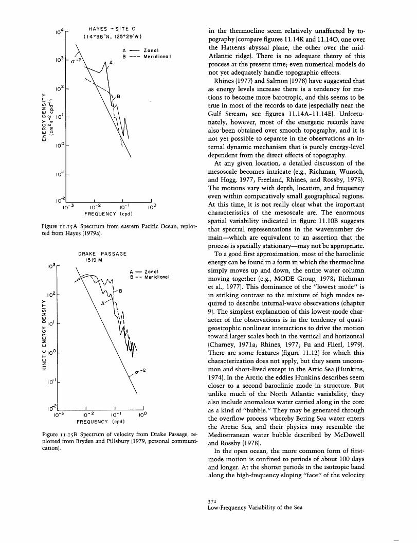
.- 4o10
102
01
100
-10
10-3
HAYES -SITE C
( 1438' N, 125029'W)
A
10- 2i
FREQUENCY
- ZonalMeridiona I
I I0-i 100
cpd)
Figure II.ISA Spectrum from eastern Pacific Ocean, replot-ted from Hayes (1979a).
DRAKE PASSAGE1519 M
ZonalMeridional
V I
10-2 10o-FREQUENCY (cpd)
100
Figure II.I B Spectrum of velocity from Drake Passage, re-plotted from Bryden and Pillsbury (1979, personal communi-cation).
in the thermocline seem relatively unaffected by to-pography (compare figures 11.14K and 11.140, one overthe Hatteras abyssal plane, the other over the mid-Atlantic ridge). There is no adequate theory of thisprocess at the present time; even numerical models donot yet adequately handle topographic effects.
Rhines (1977) and Salmon (1978) have suggested thatas energy levels increase there is a tendency for mo-tions to become more barotropic, and this seems to betrue in most of the records to date (especially near theGulf Stream; see figures 11.14A-11.14E). Unfortu-nately, however, most of the energetic records havealso-been obtained over smooth topography, and it isnot yet possible to separate in the observations an in-ternal dynamic mechanism that is purely energy-leveldependent from the direct effects of topography.
At any given location, a detailed discussion of themesoscale becomes intricate (e.g., Richman, Wunsch,and Hogg, 1977; Freeland, Rhines, and Rossby, 1975).The motions vary with depth, location, and frequencyeven within comparatively small geographical regions.At this time, it is not really clear what the importantcharacteristics of the mesoscale are. The enormousspatial variability indicated in figure 11.lOB suggeststhat spectral representations in the wavenumber do-main-which are equivalent to an assertion that theprocess is spatially stationary-may not be appropriate.
To a good first approximation, most of the baroclinicenergy can be found in a form in which the thermoclinesimply moves up and down, the entire water columnmoving together (e.g., MODE Group, 1978; Richmanet al., 1977). This dominance of the "lowest mode" isin striking contrast to the mixture of high modes re-quired to describe internal-wave observations (chapter9). The simplest explanation of this lowest-mode char-acter of the observations is in the tendency of quasi-geostrophic nonlinear interactions to drive the motiontoward larger scales both in the vertical and horizontal(Charney, 1971a; Rhines, 1977; Fu and Flierl, 1979).There are some features (figure 11.12) for which thischaracterization does not apply, but they seem uncom-mon and short-lived except in the Artic Sea (Hunkins,1974). In the Arctic the eddies Hunkins describes seemcloser to a second baroclinic mode in structure. Butunlike much of the North Atlantic variability, theyalso include anomalous water carried along in the coreas a kind of "bubble." They may be generated throughthe overflow process whereby Bering Sea water entersthe Arctic Sea, and their physics may resemble theMediterranean water bubble described by McDowelland Rossby (1978).
In the open ocean, the more common form of first-mode motion is confined to periods of about 100 daysand longer. At the shorter periods in the isotropic bandalong the high-frequency sloping "face" of the velocity
37ILow-Frequency Variability of the Sea
z a.LU o
EIL uZW
IU-
02
I-
, lozU3
Z
1OCUo
zbc
-II0
162 I
-
103 _
_
r
_
102 _
.,A
IB_
_
, _l-310-3

spectra, there is little coherence in the vertical, sug-gesting very short vertical scales, and the motion hasmuch of the character one would expect of the geo-strophic turbulence models [i.e., the horizontal kineticenergies are isotropic, the energy is partitioned equallybetween potential energy and the two kinetic energycomponents, and in the vertical the energy varies withthe buoyancy frequency N(z) (Charney, 1971a)].
The simple vertical movement of the thermoclinesuperficially resembles the lowest dynamic mode on alinear 8-plane. But a quantitative examination of itsform suggests a distortion, perhaps due to a larger scaleshear, and a coupling of several modes characteristic ofnonlinear motions (Davis, 1976; Richman et al., 1977).In the western North Atlantic, it appears that the timescales are too short to be describable by linear dynam-ics, and any hope that one could describe the low-frequency variability by a simple superposition ofRossby waves seems slight, although this has not pre-vented attempts at doing so.
On the other hand, Bernstein and White (1974) claimthat in the eastern Pacific XBT observations of theupper ocean give baroclinic signals that are consistentwith elementary Rossby-wave dispersion curves. Theirresult is agreement with the observation (Fu andWunsch, 1979) that in moored measurements in thecentral Atlantic near the mid-Atlantic Ridge the timescales appear to be longer and begin to approach thoseto which we might apply linear theory. There is asuggestion here that the westward intensification inthe eddy field-an analog of the westward intensifica-tion of the mean circulation-also may drive the eddyflow into a more nonlinear range, much as one canpostulate a nonlinear Gulf Stream in a more nearlylinear interior mean ocean flow.
The resources required to study the detailed localdynamics of the eddy field are very great and suchstudies have rarely been attempted. With the possibleexception of Gulf Stream rings, and other features inthe immediate proximity of the Gulf Stream (and bypresumption near other western boundary currents),the motions are indistinguishable from geostrophicbalance. This near-geostrophic balance, which one an-ticipates on the basis of simple scale analysis (N. A.Phillips, 1963), dominates the momentum balance andprecludes direct study of the nongeostrophic terms inthe governing equations that could lend insight intothe source and sinks of the motions. To proceed, oneis forced to study the vorticity balance that eliminatesthe lowest-order relation. Attempts along these lineshave been made for the MODE-1 data by Bryden andFofonoff (1977) and by McWilliams (1976). For thatplace at that time a specific balance can be identifiedin the quasi-geostrophic vorticity equation, although
McWilliams showed that on the average (as opposed tothe instantaneous balance) a linearized form seems towork well.
The question raised in the introduction [equations(11.1)-(11.4)] concerning the effects of variability, inparticular the mesoscale eddy field on the mean cir-culation, is difficult to answer. The large gradients ofenergy density described by Schmitz (and made obviousin the figures 11.11B and 11.14) suggest the presenceof large Reynolds-stress gradient terms of the form
a ( U ' 2), a (V'2),
where u', v' are the fluctuation-velocity components.The dynamic implications of these terms, while clearin principal, are obscure in practice because the com-plete suite of Reynolds stresses has not been measured.In the immediate vicinity of the Gulf Stream, Thomp-son (1977) has argued that the off-diagonal terms (u'v')show a convergence of momentum into the GulfStream consistent with a Rossby-wave energy flux inthe opposite direction. Away from the immediate vi-cinity of the Gulf Stream, the significance of these off-diagonal terms is not understood (a related question isthe meaning of the varying ratios of meridional andzonal energies visible in the spectra displayed here).
Eddies may also carry a heat flux through Reynoldsterms of the form (u'T'), (v'T'), etc. Except for Bryden(1979), who reports a significant poleward eddy heatflux in the Drake Passage and similar reports from theFlorida Straits, no one has succeeded in measuring sta-tistically significant eddy heat fluxes. The correlationsbetween temperature fluctuations and velocity fluc-tuations in the regions where measurements exist aresufficiently weak that it appears that much longer rec-ords will be needed to measure significant values-which, however, may be so small as to be dynamicallymeaningless. Both the Drake Passage and Florida Cur-rent results may be typical of strong jetlike currentsover topography rather than of the open sea. Many ofthe features of these two regions are similar [compareWunsch and Wimbush (1977) and Baker et al. (1977)].
The absence of significant eddy heat-flux terms alsoseems to rule out open-sea baroclinic instability as animportant source of eddy energy (Gill, Green, and Sim-mons, 1974), although the upper ocean has not beensampled adequately. Such an instability requires thatthe eddies extract available potential energy from themean flow, thus generating an eddy heat flux down themean temperature gradient. Even in the region of theAtlantic North Equatorial Current (Keffer and Niiler,1978), which had seemed a strong candidate for suchinstability (Gill, Green, and Simmons, 1974), the eddyheat-flux terms are small. One presumes such insta-bilities (or more likely a mixed barotropic-baroclinic
372Carl Wunsch
i IC·I�s�--3C · r�--C __

instability) must occur in the near-Gulf Stream regionbut the difficulties of measurement in the strong ve-locities that occur there has precluded quantitative es-timates of the heat flux-terms. (Strong mooring mo-tions induced by the high velocities produce fictitioustemperature signals coherent with the velocity field.)
If we rule out open-sea generation by meteorologyand open-sea baroclinic instability as mesoscale eddysources, we are left only with topographic generationand generation and radiation from strong boundary cur-rents as possible significant eddy sources. Both are dif-ficult to evaluate quantitatively. Schmitz (1978) andFu and Wunsch (1979) showed that the major effect oftopography seems to be the spin-down of the deepocean layers relative to the thermocline. Topographywould thus more closely resemble a sink of eddy energythan its source. At the present time, then, the strongboundary currents seem the most likely major sourceof eddy energy.
These general results, coupled with the intense con-centration of low-frequency energy near the westernboundary currents, suggests that the eddy field mayindeed be dynamically unimportant except in the im-mediate vicinity of the boundary currents. The pres-ence of a strong recirculation on the flanks of the GulfStream System (Worthington, 1976; Stommel, Niiler,and Anati, 1978; Wunsch, 1978a; Reid, 1978; and seechapter 1) is associated with an intense barotropic eddyfield (Schmitz, 1978) and a large resident population ofGulf Stream rings (Richardson, Cheney and Worthing-ton, 1978). A discussion of the Gulf Stream Systemvariability may be found in chapter 4 and will thus notbe pursued here. But at this time the only strong evi-dence for the importance of the variability in the dy-namics of the mean flow is in the western boundarycurrent regions. Theories (Pedlosky, 1977) show thatthe interior field could be largely radiated from theGulf Stream System and from moving Gulf Streamrings (Flierl, 1977; see also chapter 18).
The mesoscale and other spatial scales of variabilitybecome bound up with almost all other aspects ofoceanography, including biological, geological, andchemical as well as physical oceanography. To the ex-tent that the variability transports properties, nutrientsand other tracers can be expected to be carried along.Eddies will scour the bottom, confusing the interpre-tation of sediments, and indeed will carry sedimentswith them from one region to another, possibly quitecontrary to the overall time-mean flows. On the phys-ical side, the variability will interact with internalwaves and fine structure on the short-wavelength endof the spectrum, and there is probably an interactionbetween the mesoscale variability and the interannualfluctuations at the other end. We have not dealt di-rectly here with any of these questions; to do so would
require a complete discussion of almost all aspects ofoceanography and would be premature in any case.
11.3 Summary and Conclusions
The extent to which the ocean undergoes large-scaleclimatological fluctuations remains uncertain in theface of difficult sampling problems and the short du-ration over which appropriate instrumentation has ex-isted. Given that large fluctuations exist at least in thesea-surface temperature field, we cannot really distin-guish changes imposed by the atmosphere with a staticocean response from those in which large-scale oceanicdynamics are directly involved. Study of the atmos-pheric spectra displayed here and elsewhere suggeststhat the forcing and response by the atmosphere is acomplex function of position and time scale. With allof the current emphasis on the question of climaticchanges, we have been able to do little more thandefine what we do not know.
Study of the more accessible mesoscale is very muchin its infancy and generalizations are dangerous be-cause so little of the ocean has actually been ap-propriately sampled. At present, one can draw a fewqualitative conclusions that may survive futureobservational programs. The mesoscale eddy field ishighly inhomogeneous spatially-both in the horizon-tal and the vertical. Direct wind forcing and instabili-ties of the interior ocean are unlikely to provide muchenergy to the mesoscale. Much of the total mesoscaleenergy is found in the immediate proximity to thewestern boundary currents in the region where theyare going seaward. It seems, therefore, that these re-gions are the generators of much of the eddy field en-ergy. Detailed mechanisms are not yet known. Theintense recirculations that exist on both sides of theGulf Stream, the underlying eddy field (Luyten, 1977),and the formation and decay of Gulf Stream rings thereare probably related. They suggest an intimate relationbetween the generation of the eddy field, the mainte-nance of the eastward going jet, and the transition ofthe jet into the comparatively quiescent interior in acomplex dynamic linkage that we can only vaguelyunderstand. One would guess that the next 10 yearswill find many of the keys to these puzzles.
The spectra that are displayed throughout this papersuggest that oceanic low-frequency variability doeshave some characteristic features independent of ge-ography. An eddy-containing band between 50 and 150days is a feature of most regions. Almost all the spectrashow an isotropic band at frequencies higher than theeddy-containing band with a slope not far from -2. (Inthe immediate vicinity of topography the isotropicband may show-more structure.) The interannual bandhas a distinct tendency to zonality, especially in the
373Low-Frequency Variability of the Sea
�_��__�·

thermocline. These features are nearly independent ofthe remarkable fluctuations (two orders of magnitude)in the overall energy levels.
Although the supporting evidence is more sparse, thedominant mode of baroclinic motion in the eddy-con-taining band is a simple vertical translation of the ther-mocline with roughly isotropic horizontal velocities;lower frequencies are more zonal and confined to theupper ocean (cf. Schmitz, 1978). The isotropic band hasenergy levels nearly independent of depth when a sim-ple scaling by the buoyancy frequency is made. We aretotally ignorant of the deep structure on decadal andlonger time scales.
The connections between medium-scale oceanic var-iability and the growing interest in global climate re-main problematical. Despite the substantial effort thathas gone into understanding the large-scale surfaceanomalies in the ocean and the possibility of inducedchanges in the atmosphere, the subject remains enig-matic. Conceivably, subtle changes in the ocean areclimatologically more important. For example, onecould imagine that the changes in regional eddy statis-tics induce changes in the ocean eddy heat flux (if itexists) and thus in climate. By now the reader shouldappreciate how far we are from being able to deduceglobal estimates of the eddy statistics, much less theirtemporal fluctuations.
Obtaining a full three-dimensional description ofocean variability has remained beyond the capabilityof oceanographers to this day. A few regions have beenintensively studied for comparatively short periods (e.g.MODE Group, 1978; Brekovskikh et al., 1971) arid usehas been made of crude data sets [e.g., engine-intaketemperatures (Fieux and Stommel, 1975)] to build upa qualitative global picture. But it must be admittedthat despite the advances that have occurred duringthe past decades, perhaps our main accomplishment instudying the variability has been to come to appreciatethe magnitude of the task. We now recognize the enor-mous discrepancy between what is required to fullydescribe and understand the ocean, and the tools weare actually able to bring to bear on the problem. Thesituation is not hopeless; improvements in moored-instrument technology, new instruments (see chapter14), and entirely novel techniques, including the use ofsound (Munk and Wunsch, 1979) and of satellite sys-tems (Huang, Leitao, and Parra, 1978), suggest that thenext decade will be a period in which the descriptiveoceanography of the variability field will be built up inthe same way that a description of the mean was de-termined in the previous decades.
To conclude this chapter on a positive note we dis-play (from Wunsch and Gaposchkin, 1980) in figure11.16 the absolute sea-surface elevation and resulting
E 2.50_J
-.- 1.50
E
o -5.5C
E 2
-J
2. -I
E
U-5N -5
I -- I
I I I I I
DISTANCE KILOMETERS39.83°N 35.74°N 31.670N 27.57N 23.39°N290.98°E 293.480 E 295.74E 29783°E 299.820E
Figure i i .I6 Geostrophic velocity determined by satellite al-timetry along a track crossing Gulf Stream and Bermuda.Structure of the Gulf Stream seems plausible, as do amplitudeand space scales of surrounding eddy field. Two different av-eraging intervals are displayed. (Wunsch and Gaposchkin,1980.)
absolute surface geostrophic velocity deduced from theSEASAT-1 altimeter and the Marsh and Chang (1978)gravimetric geoid. One clearly sees the Gulf Stream,and fluctuations with the correct amplitudes and scalesfor mesoscale and larger eddies. Here at hand is a newtool, which along with others now under developmentwill allow us for the first time to attack the global fieldof variability.
374Carl Wunsch
*r - -- �---- I I I--r -T- - i _I,_ �
10