Low-frequency sea level variability and impact of recent sea icedecline on the sea level trend in the Arctic Oceanfrom a high-resolution simulation

Kai Xiao1& Meixiang Chen1

& Qiang Wang2& Xuezhu Wang1,2

& Wenhao Zhang1,2

Received: 14 November 2019 /Accepted: 8 April 2020# Springer-Verlag GmbH Germany, part of Springer Nature 2020

AbstractThe Arctic Ocean is undergoing significant changes, with rapid sea ice decline, unprecedented freshwater accumulation, andpronounced regional sea level rise. In this paper, we analyzed the sea level variation in the Arctic Ocean based on a globalsimulation with 4.5-km resolution in the Arctic Ocean using the multi-resolution Finite Element Sea Ice-OceanModel (FESOM).The simulation reasonably reproduces both the main spatial features of the sea surface height (SSH) and its temporal evolution inthe Arctic Ocean in comparison with tide gauge and satellite data. Using the model results, we investigated the low-frequencyvariability of the Arctic SSH. Both the first two dominant modes of the annual-mean SSH evolution in the Arctic Ocean presentdecadal variability and can be mainly attributed to the variability of the halosteric height, thus the freshwater content. The firstmode can be explained by the Arctic Oscillation (AO). The AO-related atmospheric circulation drives the accumulation andrelease of freshwater in the Arctic deep basin and the consequent ocean mass change over the continental shelf, leading to theantiphase changes in SSH between the shelf seas and the deep basin. The second mode shows an antiphase oscillation betweenthe two Arctic deep basins, the Amerasian and Eurasian Basins, which is driven by the Arctic dipole anomaly (DA). The DA-related wind anomaly causes a spatial redistribution of freshwater between the two basins, leading to the antiphase SSH changes.By using a dedicated sensitivity simulation in which the recent sea ice decline is eliminated, we find that the sea ice declinecontributed considerably to the observed sea level rise in the Amerasian Basin in the recent decades. Although the sea ice declinedid not change the mean SSH averaged over the Arctic Ocean, it significantly changed the spatial pattern of the SSH trend. Ourfinding indicates that both the wind regime and ongoing sea ice decline should be considered to better understand and predict thechanges in regional sea level in the Arctic Ocean.

Keywords Arctic Ocean . Sea level . FESOM .Decadal variability . Halosteric height . Sea ice decline . Freshwater content

1 Introduction

The Arctic is undergoing an unprecedented climate change,with air temperature increasing more than the global mean (a

phenomenon called Arctic amplification), significant sea iceextent and thickness reduction, Greenland ice sheet mass loss,and liquid freshwater accumulation (e.g., Proshutinsky et al.2009; Serreze et al. 2009; Wang et al. 2005; Giles et al. 2012;Wang et al. 2018a). Sea surface height (SSH) is a naturalintegral indicator of global and regional ocean climate change(Church et al. 2013). Changes of regional sea level, whichvaries on a broad range of timescales, can deviate substantiallyfrom those of the global mean. Currently, there are still largeuncertainties in the estimate of sea level changes in high lati-tudes, especially in the Arctic Oceanwhich has permanent andseasonal sea ice cover (Stammer et al. 2013).

In the Arctic Ocean, only along the Russian and Norwegiancoastlines, there are some reliable continuous tide gauge re-cords available starting from the 1950s, and a large proportionof the Russian sector tide gauge records was discontinuedaround 1990 (Proshutinsky et al. 2004; Henry et al. 2012;

This article is part of the Topical Collection on the 11th InternationalWorkshop on Modeling the Ocean (IWMO), Wuxi, China, 17-20June 2019

Responsible Editor: Tal Ezer

* Meixiang Chenchenmeixiang@hhu.edu.cn

1 College of Oceanography, Hohai University, No. 1 Xikang Road,Nanjing 210098, China

2 Alfred-Wegener-Institut Helmholtz-Zentrum für Polar- undMeeresforschung, Bremerhaven, Germany

Ocean Dynamicshttps://doi.org/10.1007/s10236-020-01373-5

Svendsen et al. 2016). Since the early 1990s, altimetric satel-lite missions have provided observations of sea level in theArctic Ocean south of 82° N, allowing extraction of primarysea level variation patterns. Although conventional processingof satellite radar altimetry breaks down in the presence of seaice, specialized satellite altimeter processing allows the extrac-tion of SSH in ice-covered areas, making the study of sea levelchanges in the ice-covered Arctic Ocean possible (Laxon1994; Peacock and Laxon 2004; Prandi et al. 2012a, 2012b;Giles et al. 2012; Cheng et al. 2015; Armitage et al. 2016;Svendsen et al. 2016; Rose et al. 2019).

Obvious sea level rise along the coast of Russian andNorwegian seas has been reported based on the tide gaugerecords (Proshutinsky et al. 2004; Henry et al. 2012). Rapidsea level rise in the Beaufort Gyre in the recent two decadeswas observed by satellite altimeter (Prandi et al. 2012b; Chenget al. 2015; Carret et al. 2017; Rose et al. 2019). Using altim-eter and Gravity Recovery and Climate Experiment (GRACE)space gravimetry data, Armitage et al. (2016) found a largeseasonal cycle of Arctic SSH dominated by halosteric changesand a secular change of SSH determined by ocean masscontributions between 2003 and 2014. Carret et al. (2017)investigated the closure of the Arctic sea level budget since2002 and found that the spatial pattern of sea level trends inthe Arctic Ocean can be explained mainly by the halostericcomponent, but the trend of the Arctic mean SSH isdominated by mass contribution. These conclusions areconsistent with the finding of Armitage et al. (2016) basedon satellite data.

Despite great success with their applications, there are stillseveral issues with the current observation datasets. First, asrevealed by Carret et al. (2017), large uncertainties exist in theavailable Arctic sea level datasets, especially in the ice-covered area and in different GRACE products. They alsoindicated that a large difference exists in the Arctic stericchange between the results calculated directly from the tem-perature and salinity data and those obtained from the differ-ence between altimetry and GRACE data. Second, the timeseries of sea level (since 1993) and ocean mass (since 2003)are not long enough to investigate the low-frequency Arcticsea level variability associated with the cyclonic and anticy-clonic regimes of atmospheric circulation described byProshutinsky and Johnson (1997), Proshutinsky et al. (2015)and the decadal sea level variability related to the ArcticOscillation (AO) or North Atlantic Oscillation (NAO) ob-served by tide gauges along the coast (Proshutinsky et al.2004; Henry et al. 2012; Calafat et al. 2013). Third, the satel-lite measurement does not cover the area north of 82° N,making it difficult to understand the sea level variability forthe whole Arctic Ocean.

Model simulations are often used to study regional andglobal sea level changes (e.g., Bindoff et al. 2007; Yin 2012;Church et al. 2013; Griffies et al. 2014; Slangen et al. 2017;

Meyssignac et al. 2017). Proshutinsky et al. (2007) revealedthat ocean-sea ice models can well reproduce the variability ofArctic coastal SSH, although the spatial patterns and trends ofthe Arctic SSH differ significantly among models. Koldunovet al. (2014) investigated the interannual-to-decadal SSH var-iability in the Arctic Ocean using an Arctic regional modelwith an 8-km horizontal resolution. The SSH variability canbe reasonably captured by their regional model, although itfailed to reproduce the positive Arctic SSH trend observedover the last two decades, which might be due to open bound-ary conditions applied to the regional model. They also foundthat higher model resolution helps to improve the simulatedspatial distribution of SSH. Using higher model resolution canbetter represent the changes in the spatial distribution of liquidfreshwater in the Arctic Ocean (Wang et al. 2016a;Wang et al.2018b). This implies that the variation of Arctic SSH could bebetter resolved with high resolution because the variation ofSSH in the Arctic Ocean contains a significant halosteric com-ponent (Morison et al. 2012; Griffies et al. 2014; Armitageet al. 2016; Carret et al. 2017).

Global simulations with the Arctic Ocean resolved with4.5-km-high resolution have become available recently(Wang et al. 2016b). Although these high-resolution simula-tions have been assessed with respect to their representation ofsea ice, ocean salinity, and temperature (Wang et al. 2018a,2018b, 2019), how well SSH in the Arctic Ocean is simulatedis not evaluated yet. In this paper, we will first assess theArctic SSH simulated in the high-resolution model setup de-scribed by Wang et al. (2018a, 2019). Then, the low-frequency variability of Arctic SSH will be investigated usingthe model results. The impact of recent Arctic sea ice declineon the Arctic SSH will also be elucidated by using a dedicatedsensitivity experiment.

The paper is organized as follows: in Section 2, we willbriefly introduce the model used in our study, as well as thesea level observations using satellites and tide gauges. We willverify simulated mean SSH and sea level variability by com-paring them with tide gauge and satellite-based SSH observa-tions in Section 3. Investigation of low-frequency sea levelvariability and its mechanism is presented in Section 4.Section 5 uses a climatology simulation to investigate theinfluence of recent rapid sea ice decline on Arctic Ocean sealevel, and Section 6 finishes with concluding remarks.

2 Model and observations

2.1 FESOM

We use the results obtained from global simulations with theFinite Element Sea Ice-Ocean Model (FESOM v.1.4, Wanget al. 2014, Danilov et al. 2015). It is an ocean general circu-lation model with both the ocean and sea ice components

Ocean Dynamics

working on unstructured triangular meshes, so it allows formulti-resolution simulations. This model has been applied andevaluated in various Arctic Ocean studies (e.g., Wang et al.2016a, 2016b, 2016c, 2018a, 2018b; Wekerle et al. 2013,2017a, 2017b; Müller et al. 2019). The model configurationused in this study is briefly described below.

The employed global mesh has 1° nominal horizontal res-olution in most parts of the world’s ocean. The resolution is setto about 24 km north of 45° N and further increased to 4.5 kmin the Arctic Ocean (defined by the Arctic gateways of theBering Strait, Canadian Arctic Archipelago (CAA), FramStrait, and Barents Sea Opening, see Fig. 1a). In the equatorialband and along the coast the resolution is also slightly in-creased. Forty-seven z levels are used with 10-m resolutionin the top 100 m and gradually coarsened downwards. Forbottom topography, we use the 2-km resolution version ofthe International Bathymetric Chart of the Arctic Ocean(IBCAO; Jakobsson et al. 2008) north of 69° N and the 1-min resolution version of the General Bathymetric Chart ofthe Oceans (GEBCO) south of 64° N. The topography is lin-early interpolated between these two data sets for the rangebetween 64° N and 69° N.

The model is driven by the 3-hourly JRA-55 atmosphericforcing (Kobayashi et al. 2015) from 1958 to 2015 (the “con-trol” run). The ocean starts from the PHC3 climatology tem-perature and salinity, and sea ice starts from the climatologicalstate obtained in a previous simulation. To understand theimpact of Arctic sea ice decline on the Arctic SSH, a sensitiv-ity experiment is carried out using climatological atmosphericthermal forcing over the Arctic Ocean (the “climatology” run).The model configuration and forcing fields are the same as inthe control run, except that the climatology of air temperatureand downward longwave and shortwave radiation is used overthe Arctic Ocean. The climatology is obtained by averaging

the JRA-55 data from 1970 to 1999 for each 3-h segment. Thissensitivity experiment branches from the control run in 2001and is run using climatological atmospheric thermal forcinguntil 2015, covering the period when the SSH in the BeaufortGyre (BG) region increased to an unprecedented level. It isshown in Wang et al. (2019) that the recent Arctic sea icedecline is well simulated by the control run and the declineis eliminated in the climatology run. Comparing the two sim-ulations will help to reveal the impacts of the sea ice declineon the Arctic SSH.

2.2 Observation data

2.2.1 Satellite altimetry

We will use the mean dynamic topography (MDT) providedby the DTU13MDT (DTU hereafter) model, which has globalcoverage with a spatial resolution of 1 min based on 20 years(1993–2012) of both altimetry and Gravity Field and Steady-State Ocean Circulation Explorer (GOCE) satellite data(Andersen et al. 2015). It is the mean sea surface referencedto the geoid, so it can be used to assess the mean SSH obtainedfrom our ocean model. Specialized satellite altimeter process-ing makes the retrieval of SSH from leads and polynyas in theice-covered area possible, and now there are monthly SSHdata from Envisat and CryoSat-2 satellites for both ice-covered and ice-free areas up to 81.5° N, as analyzed byArmitage et al. (2016). We will employ their SSH data in thispaper. This data set has a spatial coverage up to 81.5° N on a0.75° × 0.25° longitude-latitude grid for the period 2003–2014. This satellite-derived monthly SSH product has beenused for various Arctic Ocean studies (Armitage et al. 2016,2017, 2018; Regan et al. 2019).

Fig. 1 a Model horizontalresolution and b oceanbathymetry. The Arctic Ocean isenclosed by the Canadian ArcticArchipelago, Fram Strait, BarentsSea Opening, and Bering Strait(black lines). Blue lines on landrefer to the rivers flowing into theArctic Ocean. Tide gaugelocations are shown by circles,and circle colors indicate thecorrelation of the annual-meanSSH between the tide gauge andthe control simulation (see alsoTable 1)

Ocean Dynamics

2.2.2 Tide gauges

The revised local reference (RLR) tide gauge records from thePermanent Service for Mean Sea Level (PSMSL) (Holgateet al. 2013) are used for the comparisons of coastal sea levelwith our model results. Monthly data from 24 stations withinour research area are taken (Fig. 1b) and they cover most ofthe 1979–2015 period. Missing data are linearly interpolatedfor gaps that do not exceed 3 years, and stations with largergaps are not included in our study. The tide gauge data areadjusted for the influence of the glacial isostatic adjustment(GIA) using the ICE-6G/VM5a model (Peltier et al. 2015).

2.2.3 Reanalysis T-S data

The simulated steric height is compared with the values cal-culated using the objectively analyzed ocean temperature andsalinity of the EN4 data (Good et al. 2013). This data set isbased on quality-controlled ocean temperature and salinityprofiles, which consists of observational data from differentprojects to improve the Arctic data coverage.

3 Evaluation of simulated SSH

3.1 Time-mean SSH

We first compare the simulated spatial pattern of time-meanSSH with the DTU MDT for the period 1993–2012 (Fig. 2a,b, c) and with the SSH data of Armitage et al. (2016) for theperiod 2003–2014 (Fig. 2d, e, f). FESOMwell reproduces theobserved main characteristics of the SSH spatial pattern: highSSH in the Amerasian Basin with the maximum centered inthe Beaufort Sea associated with the anticyclonic BeaufortGyre and significant SSH gradients between the AmerasianBasin and Eurasian Basin associated with the Transpolar DriftStream. This implies that the model reliably reproduces themain ocean circulation pattern in the Arctic region.

There are, however, certain model biases. Compared withthe DTU data, the model underestimates the SSH north ofGreenland and in the CAA and overestimates it in the centralArctic basin (Fig. 2c). Note that large uncertainties may alsoexist in DTUMDTespecially to the north of Greenland and inthe CAA as these areas are covered by multi-year sea ice(Johannessen et al. 2014). Although the simulated mean

Fig. 2 Comparison of the mean SSH for the period 1993–2012 (a, b) and 2003–2014 (d, e). From left to right are a, d FESOM results, b DTU and eArmitage et al. (2016) observations, and c, f the residual between FESOM and observations

Ocean Dynamics

SSH for the period 2003–2014 is in better agreement with theresult of Armitage et al. (2016), there is a moderate overesti-mation in the central Arctic Ocean and underestimation inother Arctic regions (Fig. 2f). The root-mean-square error(RMSE) of the simulated SSH referenced to the observationaldata of DTU and Armitage et al. (2016) is about 9 cm. It is atthe lower bound of the error range (8–16 cm) reported inprevious studies on Arctic SSH with coarser models(Koldunov et al. 2014).

3.2 Variability of SSH

We use sea level data measured at 24 tide gauges within theArctic Ocean (Fig. 1b) to evaluate the coastal SSH variationsimulated by FESOM. The simulated SSH at the model gridpoints closest to tide gauge stations is taken, and correlationsof both the monthly and annual-mean SSH between FESOMand tide gauges are calculated to assess the seasonal and in-terannual variability. The correlation between the monthlymean data is significant for all of the tide gauge stations,varying from the lowest value of 0.32 at the Ust Kara stationlocated in the Kara Sea to the highest value of 0.92 atHonningsvag station located in the Barents Sea (Table 1).Averaged over different shelf seas, there is an excellent corre-lation in the Barents Sea (R = 0.86), Chukchi Sea (R = 0.86),and Beaufort Sea (R = 0.87). In the Kara, Laptev, and EastSiberian Seas, where the influence of seasonal runoff is thegreatest, the mean correlation is relatively smaller (0.59, 0.58,and 0.70, respectively). Our result is similar to the finding byArmitage et al. (2016), who found that monthly sea levelanomalies derived from satellite altimeters have a better cor-relation with tide gauges in the Barents and Beaufort Seas andweaker correlation in the Kara, Laptev, and East SiberianSeas. The spatial distribution of the RMSE of altimeter SSHreferenced to tide gauge data obtained in their analysis is alsosimilar to that of our simulated SSH (not shown). The meancorrelation coefficient averaged over all the stations is 0.69,indicating that the model can reasonably represent the season-al SSH variability along the Arctic coast.

The correlation of annual-mean SSH between the modeland tide gauge data is lower than the correlation of monthlymean SSH at most of the stations (Table 1). However, thecorrelation of annual-mean SSH is still significant for moststations. Except at two stations in the Kara Sea, the correlationcoefficients are in the range between 0.32 (at Nunai stationlocated in the Laptev Sea) and 0.79 (at Andreia and Fedorovastations located in the Laptev Sea and Pevek station in the EastSiberian Sea) (Fig. 1b and Table 1). The mean correlationcoefficients averaged over different regions based on annual-mean data are similar to those based on monthly data for mostshelf seas, except the Beaufort and Barents Seas, where thecorrelation is much lower on the interannual timescale. Themean correlation coefficient of annual-mean SSH averaged

over all the stations is 0.58, suggesting that the interannualSSH variability along the Arctic coast is also reasonably wellreproduced by FESOM, although slightly worse than the rep-resentation of seasonal variability.

Figure 3 a shows the anomaly of annual-mean SSH fromthe FESOM simulation and satellite observations (data fromArmitage et al. 2016) averaged over the Arctic Ocean between66° N and 81.5° N. The satellite altimetry data contains theglobal mean sea level rise caused for example by land ice lossthrough Greenland and Antarctic ice sheet melting, which isnot considered in the current simulation of FESOM. As ourinterest is in the regional dynamic sea level, the global meansea level trend was removed before the comparison. The cor-relation of the simulated annual-mean SSH with the observa-tion is 0.79, revealing that FESOM well reproduced the ob-served interannual variability of Arctic mean SSH during theperiod 2003–2014. The model shows an SSH maximum in2011, which was also reported by Armitage et al. (2016) andVolkov and Landerer (2013).

The Arctic Ocean is covered by sea ice during most time ofthe year, and sea ice coverage reaches minimum in September.In this month, the sea level observation based on satellitealtimetry has the highest accuracy and thus, we further com-pare the spatial distribution of the changing rate of theSeptember SSH from 2003 to 2014 between the model andaltimetry data (Fig. 3b). For our purpose, we computed thelinear trend to indicate the changing rate. Note that the word“trend” we used in the paper means the tendency during acertain period of analysis, which is not necessarily part ofthe long-term trend related to climate change.

The model well reproduces the spatial pattern of the SSHlinear trend, with increasing SSH in the Amerasian Basin(centered at the Beaufort Gyre) and decreasing SSH in shelfseas. Both the model and observations consistently show thatthe most pronounced SSH trends are in the western ArcticOcean, with opposite trends between the deep basin and theshelf region. The positive trends in the Amerasian Basin in themodel are slightly weaker than the observed, and the simulat-ed negative trends in the shelf seas are also weaker than theobserved, especially in the Kara and Barents Seas. The rapidsea level rise in the Beaufort Gyre has been found in manystudies (e.g., Prandi et al. 2012b, Morison et al. 2012; Chenget al. 2015; Carret et al. 2017; Rose et al. 2019) and was oftenexplained as a consequence of wind-driven freshwater accu-mulation (McPhee et al. 2009; Proshutinsky et al. 2009;Morison et al. 2012; Giles et al. 2012; Armitage et al. 2016).In Section 5, we will show that the recent sea ice declineactually contributed significantly to this sea level rise.

In conclusion, the model has a decent representation of themean SSH and its variations in the Arctic region comparedwith the tide gauge and satellite data. In the following, we willinvestigate the low-frequency SSH variability in the ArcticOcean using the model results.

Ocean Dynamics

4 Interannual-to-decadal SSH variability

Regional sea level often exhibits significant interannual-to-decadal variability with considerably high amplitude thatmay even offset the long-term global trend in a relatively shortperiod of time (e.g., Cazenave and Llovel, 2010; Stammeret al. 2013). Improved understanding of mechanisms drivingthe low-frequency sea level variability can help us to reduceuncertainties in regional sea level projections. Due to theshortness of satellite observations in the Arctic Ocean, re-search on interannual-to-decadal sea level variability in theArctic Ocean was limited to coastal regions using tide gauge

records (e.g., Proshutinsky et al. 2004; Henry et al. 2012;Calafat et al. 2013). In the following, we will use the SSHresults of FESOM to investigate the interannual-to-decadalsea level variability over the whole Arctic Ocean for the peri-od 1979–2015.

We performed an empirical orthogonal function (EOF) de-composition of the annual-mean SSH anomalies for the period1979–2015. Before the EOF decomposition, the linear trendof SSH for this period (shown in Fig. 4e) was removed fromthe time series as our focus in this analysis is on the interan-nual and decadal variability. The trend is predominantly pos-itive in the Arctic Ocean, and a small negative trend is found

Table 1 Correlations of monthlyand annual-mean FESOM andtide gauge SSH

Tide gauge Location Number (year) Correlation 1(monthly SSH)

Correlation 2(annual SSH)

Prudhoe Bay, Alaska (148.5° W, 70.4° N) 20 0.87 (0.01) 0.56 (0.01)

Beaufort Sea 20 0.87 0.56

Vrangelia (178.5° W, 71.0° N) 21 0.86 (0.01) 0.70 (0.01)

Chukchi Sea 21 0.86 0.70

Aion (168.0° E, 69.9° N) 22 0.74 (0.01) 0.78 (0.01)

Pevek (170.3° E, 69.7° N) 16 0.79 (0.01) 0.79 (0.01)

Ambarchik (162.3° E, 69.6° N) 17 0.57 (0.01) 0.73 (0.01)

Shalaurova (143.2° E, 73.2° N) 21 0.70 (0.01) 0.55 (0.01)

East Siberian Sea 19 0.70 0.71

Kigiliah (139.9° E, 73.3° N) 34 0.80 (0.01) 0.78 (0.01)

Sannikova (138.9° E, 74.7° N) 31 0.53 (0.01) 0.50 (0.01)

Kotelnyi (137.9° E, 76.0° N) 32 0.50 (0.01) 0.45 (0.01)

Dunai (124.5° E, 73.9° N) 30 0.50 (0.01) 0.32 (0.07)

Andreia (110.8° E, 76.8° N) 15 0.77 (0.01) 0.79 (0.01)

Fedorova (104.3° E, 77.7° N) 13 0.42 (0.01) 0.79 (0.01)

Tiksi (128.9° E, 71.6° N) 31 0.55 (0.01) 0.58 (0.01)

Laptev Sea 27 0.58 0.60

Zhelania II (68.6° E, 77.0° N) 14 0.53 (0.01) 0.67 (0.01)

Vise (77.0° E, 79.5° N) 24 0.62 (0.01) 0.58 (0.01)

Ust Kara (64.5° E, 69.3° N) 9 0.32 (0.01) 0.67 (0.05)

Izvestia Tsik (83.0° E, 76.0° N) 34 0.76 (0.01) 0.06 (0.72)

Golomianyi (90.6° E, 79.6° N) 27 0.52 (0.01) 0.15 (0.44)

Amderma (61.7° E, 69.8° N) 31 0.77 (0.01) 0.61 (0.01)

Kara Sea 23 0.59 0.46

Hammerfest (23.7° E, 70.7° N) 35 0.92 (0.01) 0.78 (0.01)

Honningsvag (26.0° E, 71.0° N) 33 0.92 (0.01) 0.49 (0.01)

Vardo (31.1° E, 70.4° N) 30 0.85 (0.01) 0.46 (0.01)

Krenkelia (58.1° E, 80.6° N) 11 0.73 (0.01) 0.55 (0.06)

Tromso (19.0° E, 69.6° N) 35 0.90 (0.01) 0.65 (0.01)

Barents Sea 29 0.86 0.59

Arctic Ocean 24 0.69 0.58

For each station, we show the tide gauge location; number of years available; the correlation coefficients ofmonthly and annual SSH between simulated results and tide gauge data. The values in the round brackets indicatethe significance level. The mean values for the Barents, Kara, Laptev, East Siberian, and Beaufort Seas, and thewhole Arctic Ocean are in italics

Ocean Dynamics

in the Eurasian Basin and along the coast of Alaska. The mostsignificant SSH increase is centered in the Beaufort Gyre, witha rate of more than 5 mm/year.

The first three EOFmodes of the annual-mean SSH anomalyand the corresponding principal component (PC) time series areshown in Fig. 4 a, b, and c. The first EOF (EOF1) can explain39.0% of the SSH variance, with obvious antiphase of SSHanomalies between deep basins (> 500 m) and coastal seas (<500 m) in the Arctic Ocean. The first PC (black curve inFig. 4d) shows a decadal oscillation with the turning point atthe early 1990s. This mode is consistent with the results ofKoldunov et al. (2014) and Proshutinsky and Kowalik (2007),who got a similar EOF1 pattern using data from differentmodels. This robust mode is also identified in the observedSSH based on recent satellite measurements by Armitageet al. (2018). They find that there are opposing responses ofsea level between deep basins and coastal seas during positiveand negative Arctic Oscillation (AO, Thompson and Wallace1998) events. The AO is mainly in a positive phase before the1990s and shifts to a negative phase since the mid-1990s. Thevariation in the PC1 coincides with this change, indicating thatthe relationship between this SSH mode and the AO staterevealed for the short satellite period by Armitage et al.(2018) might be valid for much longer periods. The second

EOF explains about 14.6% of the SSH variance. It shows adecadal oscillation of SSH with antiphase between theAmerasian and Eurasian Basins. The spatial pattern of thismode suggests that the Arctic atmospheric dipole anomaly(DA) might be the driving mechanism. The DA is the secondmode of the Arctic sea level pressure (SLP) first proposed byWu et al. (2006) and further linked to the Arctic sea ice minima,sea ice export, and recent sea ice decline (Wang et al. 2009; Leiet al. 2015, 2016). The third mode explains 8.9% of the SSHvariance and shows an oscillation between the Russian coastwith part of the deep basin and the rest of the Arctic Ocean,which may be related to the Arctic basin-scale natural decadaloscillation in terms of first baroclinic Kelvin wave, as discussedin depth by Ikeda (1990) and Wang et al. (2005). As the firsttwo EOF modes explain the majority of the SSH variability, inthis study, we will focus on these two modes.

According to the evolution of the PC1 time series, we an-alyzed the changes of SSH and its components during theperiods of 1979–1993 and 1994–2010 separately, as they aretwo successive periods with dramatic and inverse sea levelchanges. The period 1979–1993 shows a decrease of SSH inthe central Arctic Ocean and an increase of SSH on the con-tinent shelf (Fig. 5a). A similar pattern of SSH trends appearsin 1994–2010 (Fig. 5e) but with signs opposite to the period of1979–1993. In order to explore the cause of the SSH changesduring the two periods, we further analyze the changes ofsteric height and ocean mass, which contribute to the totalSSH changes together. The steric height is separated into thehalosteric and thermosteric parts.

It is clear that the halosteric component (Fig. 5 b and f)explains most of the SSH changes, especially in the deepbasin. This can be explained by the fact that changes in seawater density in the Arctic Ocean are mainly determined bysalinity due to the low thermal expansion coefficient at lowtemperature and large haline contraction coefficient at rela-tively lower salinity (Griffies et al. 2014). The thermostericcomponent (Fig. 5 c and g) contributes very little to the totalSSH changes in the studied region. The trends of halostericand thermosteric heights are opposite in the Eurasian Basin.The decadal variability of Atlantic Water inflow, which iswarm and saline, could be responsible for this phenomenon(Dmitrenko et al. 2008). Ocean mass changes (Fig. 5 d and h)have a little contribution in the deep basin but are relativelyimportant on the continental shelf. The oceanmass changes onthe shelf in the two periods are opposite and they are linked tothe SSH changes in the central Arctic. When SSH decreases inthe central Arctic, the divergence of surface freshwater meanspiling of the water onto the shelf, thus increasing the oceanmass there (Fukumori et al. 2015; Armitage et al. 2018). Thetwo periods are characterized by opposite changes in the SSHin the deep Arctic basin, so the changes in the ocean mass onthe continental shelf are also opposite. Overall, for the long-term variability of SSH in the Arctic Ocean, the changes in the

Fig. 3 a Anomaly of annual-mean SSH from observations and FESOMaveraged over the Arctic Ocean between 66° N and 81.5° N. b, c Spatialdistribution of the rate of SSH change (linear trend) for September be-tween 2003 and 2014. The satellite altimeter data is described inArmitageet al. (2016). Global mean sea level trend has been removed. The contourlines show the 95% confidence level

Ocean Dynamics

halosteric height play a dominant role, while the consequentmass changes are relatively important in the shelf seas. Thehalosteric changes in the deep basin and the opposite masschanges over the shelf together lead to the dominant moderevealed by the EOF1 (Fig. 4a).

Since there is no continuous three-dimensional temperatureand salinity observation that covers the whole Arctic Ocean,we compute steric changes from the objectively analyzed EN4dataset to assess the steric changes calculated based on themodel output. Figure 6 shows the trends of steric height

Fig. 4 a, b, c The first 3 EOFmodes of the detrended annual-mean SSH and d the corresponding PC time series for the period 1979–2015. e The spatialdistribution of the SSH linear trend for the same period. The black contour lines show the 95% confidence level

Fig. 5 Linear trends of the SSH and its different components for a, b, c, d1979–1993 and e, f, g, h 1994–2010 simulated by FESOM. From left toright: total SSH trend, trend of halosteric height, trend of thermosteric

height, and trend of ocean bottom pressure. The black contour lines showthe 95% confidence level

Ocean Dynamics

derived from EN4 and FESOM simulations for the same pe-riods. Despite limited T-S profiles in the Arctic Ocean includ-ed in the EN4 dataset, the steric changes from the modeloutput and EN4 data share some similarities. Both of themshow negative trends in the Amerasian Basin in the earlyperiod and positive trends in the later period. However, thereis a difference in the details of the spatial patterns. The maindifference is in the eastern Eurasian Basin, where only themodel has strong negative or positive trends. In theAmerasian Basin, the strong trends are located farther fromthe coast in the model. The difference between the model andthe EN4 data could be due to biases in the spatial pattern ofsalinity in both datasets.

As the decadal variability of halosteric height dominatesthe low-frequency variability of the SSH, changes in theArctic liquid freshwater content (FWC) can serve as a keyindicator for the SSH changes. Observations have shown thatthe Arctic liquid FWC has been increasing since the mid-1990s (Proshutinsky et al. 2009; McPhee et al. 2009; Gileset al. 2012; Polyakov et al. 2013), which is mainly due to thefreshwater accumulation in the Amerasian Basin (Rabe et al.2014). The FWC variability in the Beaufort Gyre andAmerasian Basin was suggested to be forced by the wind-driven convergence/divergence (Proshutinsky et al. 2002,2015; Giles et al. 2012). Meanwhile, the FWC change of theArctic Ocean is also connected with the freshwater exchangebetween the Arctic Ocean and the Atlantic and Pacific Oceans

(Woodgate et al. 2012; Armitage et al. 2018). To understandthe decadal halosteric height variability in the Arctic Ocean,we calculate the total liquid FWCwithin the Arctic Ocean andthe total liquid freshwater transport (FWT) (positive into theArctic Ocean) across the gateway transects defined inSection 1. FWC and FWT are calculated according toEqs. (1) and (2):

FWC ¼ ∭D

Sref−SSref

dxdydz ð1Þ

FWT ¼ ∬ASref−Sð ÞSref

VndA ð2Þ

where Sref = 34.8 is the reference salinity, S is salinity, andD isthe depth where salinity is equal to the reference salinity. Aand Vn in Eq. (2) denote the area of the transect and velocitynormal to the transect. Wang et al. (2019) showed that theArctic liquid FWC in the simulation used in this paper is invery good agreement with observations (Fig. 3 in their paper).

The AO is the leading mode of the SLP variability for theextratropical Northern Hemisphere (Thompson and Wallace1998), which influences not only the sea ice but also the oceanstate. It drives the decadal Arctic sea ice oscillation (e.g.,Wang and Ikeda 2000, 2001; Ikeda et al. 2001; Wang et al.2005) and the Arctic FWC changes as well (Proshutinskyet al. 2015; Armitage et al. 2018). The impact of the AO onthe FWC can explain the dominant mode of the SSH variabil-ity shown in Fig. 4a. Here we hypothesize that the influence ofthe AO-related wind forcing on FWC will accumulate overtime. Indeed, the cumulative sum of the AO index since 1979is well correlated with the liquid FWC in the Arctic deep basin(the correlation coefficient is − 0.77 at the 0.01 significancelevel, Fig. 7a). Both of them show decadal variability with aturning point at about 1994, suggesting that this variabilityexplains the dominant mode of the SSH variability shown inFig. 4a. Because of the long memory of the ocean to the windforcing, the status of the FWC and SSH in a certain year is theconsequence of not only the ongoing atmospheric forcingchange but also the accumulative effect of the forcing in thepast. We also found that the decadal change of the liquid FWCin the Arctic deep basin is well correlated with the total liquidfreshwater transport through the Arctic gateways (the correla-tion coefficient is 0.92 at the 0.01 significance level, Fig. 7a).The correlation between the liquid freshwater transport andthe SSH is opposite between the deep basin and the shelfregion (Fig. 7b). When AO is in the negative phase, the anom-alous anticyclonic atmospheric circulation accumulates fresh-water towards the deep basin and increases the halostericheight and thus SSH in the deep basin. The associated releaseof freshwater from the continental shelf reduces the oceanmass and thus SSH in the Arctic marginal seas. The latterchanges the SSH gradient with the sub-Arctic seas and furthercauses a positive anomaly in the freshwater transport to the

Fig. 6 Trend of total steric height for a, c 1979–1993 and b, d 1994–2010: a, b EN4 data and c, d FESOM simulation. The contour lines showthe 95% confidence level

Ocean Dynamics

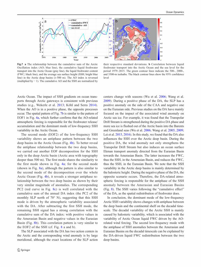
Arctic Ocean. The impact of SSH gradients on ocean trans-ports through Arctic gateways is consistent with previousstudies (e.g., Wekerle et al. 2013; Köhl and Serra 2014).When the AO is in a positive phase, the opposite processesoccur. The spatial pattern of Fig. 7b is similar to the pattern ofEOF1 in Fig. 4a, which further confirms that the AO-relatedatmospheric forcing is responsible for the freshwater release/accumulation and the dominant mode of low-frequency SSHvariability in the Arctic Ocean.

The second mode (EOF2) of the low-frequency SSHvariability shows an antiphase pattern between the twodeep basins in the Arctic Ocean (Fig. 4b). To better revealthe antiphase relationship between the two deep basins,we carried out another EOF decomposition for the SSHonly in the deep Arctic basin (Arctic area with topographydeeper than 500 m). The first mode shares the similarity tothe first mode shown in Fig. 4a; for the second mode(shown in Fig. 8a), although the pattern is also similar tothe second mode of the decomposition over the wholeArctic Ocean (Fig. 4b), it reveals a stronger antiphase re-lationship between the two deep basins as shown by theirvery similar magnitude of anomalies. The correspondingPC2 (red curve in Fig. 8c) is well correlated with thecumulative sum of the annual DA index (the PC2 of themonthly SLP north of 70° N), suggesting that this SSHmode is driven by the atmospheric variability associatedwith the DA. After subtracting the first SSH mode, theremaining SSH signal has a strong correlation with thecumulative sum of the DA index: with positive values inthe Amerasian Basin and negative values in the EurasianBasin (Fig. 8b). This correlation pattern is very similar tothe EOF2 of the SSH (cf. Fig. 8 a and b).

The SLP associated with the DA has two action centers inthe Arctic and the corresponding wind anomaly is by largemeridional, although the exact locations of the SLP action

centers change with seasons (Wu et al. 2006; Wang et al.2009). During a positive phase of the DA, the SLP has apositive anomaly on the side of the CAA and negative oneon the Eurasian side. Previous studies on the DA have mainlyfocused on the impact of the associated wind anomaly onArctic sea ice. For example, it was found that the TranspolarDrift Stream is strengthened during the positive DA phase andmore sea ice is flushed out of the Arctic basin into the Barentsand Greenland seas (Wu et al. 2006; Wang et al. 2005, 2009;Lei et al. 2015, 2016). In this study, we found that the DA alsoinfluences the SSH over the Arctic deep basin. During thepositive DA, the wind anomaly not only strengthens theTranspolar Drift Stream but also induces an ocean surfaceEkman transport anomaly directed from the Eurasian Basintowards the Amerasian Basin. The latter increases the FWC,thus the SSH, in the Amerasian Basin, and reduces the FWC,thus the SSH, in the Eurasian Basin. We note that the SSHvariability in the Arctic deep basins is mainly determined bythe halosteric height. During the negative phase of the DA, theopposite scenario occurs. Therefore, the DA-related atmo-spheric forcing is responsible for the antiphase of the SSHanomaly between the Amerasian and Eurasian Basins(Fig. 8). The SSH varies following the “cumulative effect”of the DA, as the spatial redistribution of freshwater does.

In conclusion, the dominant mode of the low-frequencyArctic SSH variability shows changes with antiphase betweenthe deep basin and the continental shelf on the decadal time-scale. The decadal variability of the Arctic SSH is mainlycaused by halosteric variability, which is associated with thevariability of Arctic Ocean liquid FWC driven by the AO-related wind forcing. The second low-frequency mode withthe antiphase of SSH anomalies between the Amerasian andEurasian Basins on the decadal timescale can be explained bythe DA-driven liquid FWC redistribution between the twodeep basins.

Fig.7 a The relationship between the cumulative sum of the ArcticOscillation index (AO; blue line), the cumulative liquid freshwatertransport into the Arctic Ocean (gray line), the liquid freshwater content(FWC; black line), and the average sea surface height (SSH; bright blueline) in the Arctic deep basins (> 500 m). The AO index is reversed(multiplied by − 1). The cumulative AO and the SSH are normalized by

their respective standard deviations. b Correlation between liquidfreshwater transport into the Arctic Ocean and the sea level for theperiod 1979–2015. The green contour lines indicate the 500-, 2000-,and 3500-m isobaths. The black contour lines show the 95% confidencelevel

Ocean Dynamics

5 Impacts of recent sea ice declineon the Arctic sea level change

The Arctic SSH has strong low-frequency variability, asdiscussed in Section 4. However, since the 2000s, signifi-cant sea level rise has been observed in the Beaufort Gyreregion, which is associated with freshwater accumulation(Giles et al. 2012; Morison et al. 2012; Long et al. 2012;Armitage et al. 2016). Meanwhile, significant sea ice de-cline has been observed in the last two decades (Kwoket al. 2009; Stroeve et al. 2012; Laxon et al. 2013). Seaice decline can influence not only the freshwater budgetthrough meltwater but also the ocean surface stress(Martin et al. 2014). Although the recent sea ice declineincreases the FWC in the Beaufort Gyre significantly(Wang et al. 2018b), it reduces the FWC in the EurasianBasin (Wang et al. 2019), which implies further impacts onthe SSH. In this section, we will quantify the impacts of therecent sea ice decline on the SSH in the Arctic Ocean usingmodel simulations. In the climatology run, the Arctic seaice decline is eliminated. The variation of the SSH in thisrun is then mainly due to wind forcing, and the differencebetween the control run and the climatology run can revealthe impacts of sea ice decline on the SSH.

We found two completely different patterns of SSH trendsin the Arctic Ocean over the studied period for the control runand climatology run (Fig. 9 a and b). Although the control runshows significant positive trends in the Amerasian Basin, asexpected from satellite observations (e.g., Prandi et al. 2012b;Cheng et al. 2015; Armitage et al. 2016; Carret et al. 2017;Rose et al. 2019) and ocean hydrography (Rabe et al. 2014),positive trends in the climatology run are rather located in theEurasian Basin and the central Arctic over the period consid-ered. The sea ice decline leads to an increase in the SSH in theAmerasian Basin and a decrease in the Eurasian Basin.

In the Amerasian Basin, the sea level has an increasingtendency until 2008 in both simulations. Afterwards, it con-tinues to rise and retain at a high level in the control run butdeclines in the climatology run (Fig. 9d). In the EurasianBasin, the sea level in the control run decreases after 2004while in the climatology run it increases (Fig. 9e). However,the mean SSH averaged over the whole deep basin is similarbetween the control and climatology runs (Fig. 9f), and themean SSH averaged over the entire Arctic Ocean includingthe coastal seas also has little difference between the runs(Fig. 9g). This means that the recent sea ice decline signifi-cantly changes the spatial pattern of SSH, although it does notchange the mean SSH over the Arctic Ocean.

Fig. 8 a The second EOF modeof the detrended annual-meanSSH in the Arctic deep basin (areadeeper than 500 m) for the period1979–2015. b The correlationbetween the cumulative sum ofthe dipole anomaly (DA) indexand the sea level with its firstmode of EOF subtracted for theperiod 1979–2015. The greencontour lines indicate the 500-,2000-, and 3500-m isobaths. Theblack contour lines show the 95%confidence level. c Time series ofthe cumulative sum of the DAindex and the PC2 of the SSH inthe Arctic deep basin. Both arenormalized by their respectivestandard deviations. The correla-tion coefficient is 0.54 at the 0.01significance level

Ocean Dynamics

The response of the SSH in the two Arctic basins to the seaice decline is consistent with the impacts of the sea ice declineon the liquid FWC spatial distribution revealed byWang et al.(2019). They found that the sea ice decline contributes tochanges in liquid FWC in the Arctic Ocean in two ways.First, sea ice meltwater reduces the upper ocean salinity, thusincreasing the Arctic Ocean liquid FWC. Second, the reduc-tion in sea ice thickness and concentration increases the oceansurface stress, which is in favor of the export of upper-oceanwater masses from the Siberian Shelf and the Eurasian Basintowards the Amerasian Basin in the studied period. Alongwith the retreat of Pacific Water to the American Basin, theproportion of brine Atlantic Water in the upper ocean of theEurasian Basin increases. The increase of liquid FWC in theAmerasian Basin is nearly compensated by the reduction inthe Eurasian Basin. As a result, the total Arctic liquid FWC is

almost unchanged with the sea ice decline, but the spatialdistribution of the FWC is changed considerably. As theArctic Ocean SSH variability is dominated by the variabilityof the halosteric height, the changes of liquid FWC inducedby the sea ice decline reported by Wang et al. (2019) wellexplain the impacts of the sea ice decline on the SSH shownin Fig. 9: it increases the SSH in the Amerasian Basin andreduces the SSH in the Eurasian Basin. Morison et al. (2012)observed a dipole pattern in the change of Arctic SSH be-tween 2005 and 2008, with a decrease in the SSH in theEurasian Basin and an increase in the Amerasian Basin. Asthe wind forcing is the same in our two simulations, the factthat such an opposite change is only present in the control runand not in the climatology run (see Fig. 9d, e) indicates thatthe sea ice decline is responsible for the observed dipolepattern of the SSH change.

Fig. 9 a, b, c SSH trends for the period 2001–2015 from control andclimatology runs and the difference between the two simulations. Theblack contour lines show the 95% confidence level. d, e, f, g Anomaly

of SSH in the Amerasian Basin, Eurasian Basin, Arctic deep basin (sumof the two basins), and the entire Arctic Ocean in the control and clima-tology simulations

Ocean Dynamics

6 Conclusions

In this paper, we studied the regional dynamical sea levelvariability in the Arctic Ocean in the period 1979–2015using the FESOM simulations. FESOM reasonably repro-duces the main spatial pattern of the mean sea surfaceheight (SSH) in the Arctic Ocean over the period 1993–2012 compared with the DTU13MDT data and over theperiod 2003–2014 compared with the satellite altimetry da-ta derived by Armitage et al. (2016). Furthermore, the SSHsimulated by FESOM has a good correlation with both tidegauge data and the SSH based on satellite altimetry aver-aged over the Arctic Ocean. It can also reproduce the rapidsea level rise in the Amerasian Basin observed in the lasttwo decades by the altimeter.

To understand the low-frequency variability of the ArcticSSH, we carried out an EOF analysis of the detrended annual-mean SSH. The first mode shows an obvious decadal oscilla-tion with the SSH having opposite anomalies in the deep basinand coastal seas. The SSH has a turning point in 1994. In theperiod 1979–1993, the SSH decreased in the deep basin andincreased over the continental shelf; in the period 1994–2010,the SSH increased in the deep basin and decreased over thecontinental shelf. The decadal SSH variability in the deepbasin can bemainly attributed to the halosteric height variabil-ity, which is manifested in the variability of liquid FWC.

The first mode of the SSH in the Arctic Ocean is associatedwith the Arctic Oscillation (AO). The AO drives the decadalvariability of the FWC in the Arctic deep basin, thus the var-iability of the SSH. When AO is predominantly in a negativephase (anomalous anticyclonic winds), as in the period 1994–2010, surface freshwater is converged towards the Arctic deepbasin and the FWC increases, leading to an increase in theSSH in the deep basin. Contemporarily, the release of watermasses frommarginal seas towards the deep basin reduces theocean mass, thus reducing the SSH, over the continental shelf.The reduction of SSH in the periphery of the Arctic Oceanallows for a positive anomaly in the net freshwater transportinto the Arctic Ocean.

The second mode of the low-frequency SSH variability hasanomalies with antiphase between the Amerasian andEurasian Basins on the decadal timescale, which can be ex-plained by the Arctic dipole anomaly (DA). The wind anom-aly associated with the DA redistributes freshwater betweenthe two deep basins, leading to the antiphase SSH variabilityin the two deep basins.

The significant sea level rise in the Amerasian Basin inrecent decades has been mainly attributed to the anticy-clonic winds in previous studies (e.g., Proshutinsky et al.2002, 2015; Giles et al. 2012), which accumulate freshwa-ter through convergence and Ekman downwelling. Byusing a dedicated sensitivity simulation in which theArctic sea ice decline is eliminated, in this study, we

identified that the recent sea ice decline has contributedconsiderably to the increasing SSH in the AmerasianBasin. Although the sea ice decline did not change themean SSH averaged over the whole Arctic Ocean, it sig-nificantly increased the SSH in the Amerasian Basin butreduced the SSH in the Eurasian Basin. The effect of thesea ice decline on the SSH is associated with its impacts onthe spatial distribution of liquid FWC reported by Wanget al. (2019). They found that the sea ice decline increasesthe FWC in the Amerasian Basin by both supplying melt-water and shifting the freshwater from the Eurasian Basintowards the Amerasian Basin. The FWC in the EurasianBasin is consequently reduced. The corresponding changesin the halosteric height thus result in the opposite changesin the SSH in the two Arctic basins. Our results addressedthat the impacts of sea ice decline on the regional sea levelchange in the Arctic Ocean should not be neglected whenstudying or predicting sea level changes.

Our study revealed two processes that can lead to SSHvariations with antiphase between the two Arctic deep basins.One is the wind variability (atmospheric momentum forcing)associated with the DA, and the other is the decline of Arcticsea ice (atmospheric thermal forcing). In certain periods, theantiphase variability can be directly observed (e.g., Morisonet al. 2012). However, the AO-driven variability may masksuch antiphase variability sometimes. By using EOF decom-position and dedicated numerical experiments, wedisentangled these processes and explicitly illustrated theirimportance in determining the regional sea level change inthe Arctic Ocean.

The numerical simulations in this study facilitated toimprove our understanding of the variability and trendsof the SSH in the Arctic Ocean. Although the model per-forms relatively well compared with available observa-tions, it shows certain biases in the details of the spatialpatterns of the mean SSH and its trend. The resultsdiscussed in this paper also provide useful informationfor future model development.

Acknowledgments We are very thankful to the Technical University ofDenmark (DTU) for sharing the mean dynamic topography data ofMTD13DTU (ftp.space.dtu.dk/pub/DTU13/). Arctic sea level anomalydata are provided by the Centre for Polar Observation and Modelling,University College London (www.cpom.ucl.ac.uk/dynamic_topography)(Armitage et al. 2016, 2017). Tide gauge data are from the PermanentService for Mean Sea Level (http://www.psmsl.org/). EN4.2.1 griddedprofiles are from Met Office Hadley Center (https://www.metoffice.gov.uk/hadobs/en4/). We thank the anonymous reviewers and the editor fortheir very helpful comments.

Funding information The study is financially supported by the NationalKey Research and Development Program of China (Grant2017YFA0604600) and the National Natural Science Foundation ofChina (nos. 41576020, 41506006, 41376028, 41676019, and41976163). QW is supported by the German Helmholtz ClimateInitiative REKLIM (Regional Climate Change).

Ocean Dynamics

References

Andersen O, Knudsen P, Stenseng L (2015) The DTU13MSS (Mean SeaSurface) and MDT (Mean Dynamic Topography) from 20 Years ofSatellite Altimetry. In: Jin S, Barzaghi R (eds) IGFS 2014.International Association of Geodesy Symposia, vol 144. Springer,Cham

Armitage T, Bacon S, Kwok R (2018) Arctic sea level and surface circu-lation response to the Arctic oscillation. Geophys Res Lett 45:6576–6584. https://doi.org/10.1029/2018GL078386

Armitage T, Bacon S, Ridout A, Petty A,Wolbach S, TsamadosM (2017)Arctic Ocean surface geostrophic circulation 2003-2014.Cryosphere 11(4):1767–1780. https://doi.org/10.5194/tc-11-1767-2017

Armitage T, Bacon S, Ridout A, Thomas S, Aksenov Y, Wingham D(2016) Arctic sea surface height variability and change from satelliteradar altimetry and GRACE, 2003-2014. J Geophys Res Oceans121:4303–4322. https://doi.org/10.1002/2015JC011579

Bindoff N, Willebrand J, Artale V et al (2007) Observations: Oceanicclimate change and sea level. Climate Change 2007: The PhysicalScience Basis. S. Solomon et al. Eds, Cambridge University Press,386–432

Calafat F, Chambers D, Tsimplis M (2013) Inter-annual to decadal sea-level variability in the coastal zones of the Norwegian and Siberianseas: the role of atmospheric forcing. J Geophys Res Oceans 118:1287–1301. https://doi.org/10.1002/jgrc.20106

Carret A, Johannessen J, Andersen O, Ablain M, Prandi P, Blazquez Aet al (2017) Arctic sea level during the satellite altimetry era. SurvGeophys 38(1):251–275

Cazenave A, Llovel W (2010) Contemporary sea level rise. Annu RevMar Sci 2:145–173

Cheng Y, Andersen O, Knudsen P (2015) An improved 20-year arcticocean altimetric sea level data record. Mar Geod 38:146–162

Church J, Clark P, Cazenave A et al (2013) Sea level change. In: Climatechange 2013: the physical science basis. Contribution of workinggroup I to the fifth assessment report of the intergovernmental panelon climate change. Cambridge University Press, Cambridge andNew York, pp 1137–1216

Danilov S, Wang Q, Timmermann R, Iakovlev N, Sidorenko D,Kimmritz M, Jung T, Schröter J (2015) Finite-element sea ice model(FESIM), version 2. Geosci Model Dev 8:1747–1761

Dmitrenko I, Kirillov S, Tremblay L (2008) The long-term and interan-nual variability of summer fresh water storage over the easternSiberian shelf: implication for climatic change. J Geophys Res113:C03007. https://doi.org/10.1029/2007JC004304

Fukumori I, Wang O, Llovel W, Fenty I, Forget G (2015) A near-uniformfluctuation of ocean bottom pressure and sea level across the deepocean basins of the Arctic Ocean and the Nordic seas. ProgOceanogr 134:152–172

Giles K, Laxon S, Ridout A,WinghamD, Bacon S (2012)Western ArcticOcean freshwater storage increased by wind-driven spin-up of theBeaufort Gyre. Nat Geosci 5:194–197. https://doi.org/10.1038/ngeo1379

Good S, Martin M, Rayner N (2013) EN4: quality controlled ocean tem-perature and salinity profiles and monthly objective analyses withuncertainty estimates. J Geophys Res Oceans 118(12):6704–6716.https://doi.org/10.1002/2013JC009067

Griffies S, Yin J, Durack P et al (2014) An assessment of global andregional sea level for years 1993–2007 in a suite of interannualCORE-II simulations. Ocean Model 78:35–89

Henry O, Prandi P, Llovel W, Cazenave A, Jevrejeva S, Stammer D,Meyssignac B, Koldunov N (2012) Tide gauge-based sea level var-iations since 1950 along the Norwegian and Russian coasts of theArctic Ocean: contribution of the steric and mass components. JGeophys Res 117:C06023. https://doi.org/10.1029/2011JC007706

Holgate S, Matthews A, Woodworth P et al (2013) New data systems andproducts at the permanent service for mean sea level. J Coast Res29(3):493–504. https://doi.org/10.2112/JCOASTRES-D-12-00175.1

Ikeda M (1990) Decadal oscillation of the air-ice-sea system in the north-ern hemisphere. Atmos Ocean 28:106–139

Ikeda M, Wang J, Zhao JP (2001) Hypersensitive decadal oscillations inthe Arctic/subarctic climate. Geophys Res Lett 28(7):1275–1278

Jakobsson M, Macnab R, Mayer L et al (2008) An improved bathymetricportrayal of the Arctic Ocean: implications for ocean modeling andgeological, geophysical and oceanographic analyses. Geophys ResLett 35:L07602. https://doi.org/10.1029/2008GL033520

Johannessen J, Raj R, Nilsen J et al (2014) Toward improved estimationof the dynamic topography and ocean circulation in the high latitudeandArctic Ocean: the importance of GOCE. Surv Geophys 35(3):1–19

Kobayashi S, Ota Y, Harada Y et al (2015) The JRA-55 reanalysis: gen-eral specifications and basic characteristics. J Meteorol Soc Jpn SerII 93(1):5–48. https://doi.org/10.2151/jmsj.2015-001

Köhl A, Serra N (2014) Causes of decadal changes of the freshwatercontent in the Arctic Ocean. J Clim 27:3461–3475. https://doi.org/10.1175/JCLI-D-13-00.389.1

Koldunov N, Serra N, Köhl A et al (2014) Multimodel simulations ofArctic Ocean sea surface height variability in the period 1970–2009.J Geophys Res Oceans 119(12):8936–8954. https://doi.org/10.1002/2014JC010170

Kwok R, Cunningham G, Wensnahan M et al (2009) Thinning and vol-ume loss of the Arctic Ocean sea ice cover: 2003–2008. J GeophysRes 114:C07005. https://doi.org/10.1029/2009JC005312

Laxon S (1994) Sea ice altimeter processing scheme at the EODC. Int JRemote Sens 15 :915–924 . h t tps : / / do i . o rg /10 .1080 /01431169408954124

Laxon S, Giles K, Ridout A et al (2013) CryoSat-2 estimates of Arctic seaice thickness and volume. Geophys Res Lett 40(4):732–737. https://doi.org/10.1002/grl.50193

Lei R, Heil P, Wang J, Zhang Z, Li Q, Li N (2016) Characterization ofsea-ice kinematic in the Arctic outflow region using buoy data. PolarRes 35:22658

Lei R, Leppäranta M, Wang J et al (2015) Changes in sea ice along theArctic northeast passage since 1979: results from remote sensingdata. Cold Reg Sci Technol 119:132–144

Long Z, Perrie W, Tang CL, Dunlap E, Wang J (2012) Simulated inter-annual variations of freshwater content and sea surface height in theBeaufort Sea. J Clim 25(4):1079–1095. https://doi.org/10.1175/2011JCI14121.1

Martin T, Steele M, Zhang J (2014) Seasonality and long term trend ofArctic Ocean surface stress in a model. J Geophys Res Oceans 119:1723–1738. https://doi.org/10.1002/2013JC009425

McPheeM, Proshutinsky A,Morison J, Steele M, Alkire M (2009) Rapidchange in freshwater content of the Arctic Ocean. Geophys Res Lett36:L10602. https://doi.org/10.1029/2009GL037525

Meyssignac B, Slangen A, Melet A et al (2017) Evaluating model simu-lations of twentieth-century sea-level rise. Part II: regional sea-levelchanges. J Clim 30(21):8565–8593

Morison J, Kwok R, Peralta-Ferriz C, Alkire M, Steele M (2012)Changing arctic ocean freshwater pathways. Nature 481(7379):66–70

Müller F, Wekerle C, Dettmering D, Passaro M, Bosch W, Seitz F (2019)Dynamic ocean topography of the northern Nordic seas: a compar-ison between satellite altimetry and ocean modeling. Cryosphere 13:611–626

PeacockN, Laxon S (2004) Sea surface height determination in the ArcticOcean from ERS altimetry. J Geophys Res Oceans 109:C07001.https://doi.org/10.1029/2001JC001026

Ocean Dynamics

Peltier W, Argus D, Drummond R (2015) Space geodesy constrains iceage terminal deglaciation: the global ice-6g_c (vm5a) model. JGeophys Res Solid Earth 120(1):450–487

Polyakov I, Bhatt U,Walsh J, Abrahamsen E, PnyushkovA,Wassmann P(2013) Recent oceanic changes in the Arctic in the context of long-term observations. Ecol Appl 23(8):1745–1764. https://doi.org/10.1890/11-0902.1

Prandi P, Ablain M, Cazenave A, Picot N (2012a) Sea level variability inthe Arctic Ocean observed by satellite altimetry. Ocean Sci Discuss9(4):2375–2401. https://doi.org/10.5194/osd-9-2375-2012

Prandi P, Ablain M, Cazenave A, Picot N (2012b) A new estimation ofmean sea level in the Arctic Ocean from satellite altimetry. MarGeod 35(sup1):61–81. https://doi.org/10.1080/01490419.2012.718222

Proshutinsky A, Ashik I, Dvorkin E, Häkkinen S, Krishfield R, Peltier W(2004) Secular sea level change in the Russian sector of the ArcticOcean. J Geophys Res Oceans 109:C03042. https://doi.org/10.1029/2003JC002007

Proshutinsky A, Ashik I, Häkkinen S et al (2007) Sea level variability inthe Arctic Ocean from AOMIP models. J Geophys Res Oceans 112:C04S08. https://doi.org/10.1029/2006JC003916

Proshutinsky A, Bourke R, Mclaughlin F (2002) The role of the BeaufortGyre in Arctic climate variability: seasonal to decadal climate scales.Geophys Res Lett 29(23):2100

Proshutinsky A, Dukhovskoy D, Timmermans ML, Krishfield R,Bamber JL (2015) Arctic circulation regimes. Phil Trans R Soc A373:20140160. https://doi.org/10.1098/rsta.2014.0160

Proshutinsky A, Johnson M (1997) Two circulation regimes of the wind-driven Arctic Ocean. J Geophys Res 102(C6):12493–12514

Proshutinsky A, Krishfield R, Timermans M et al (2009) Beaufort Gyrefreshwater reservoir: state and variability from observations. JGeophys Res Oceans 114:C00A10. https://doi.org/10.1029/2008JC005104

Proshutinsky A, Kowalik Z (2007) Preface to special section on ArcticOcean model intercomparison project (AOMIP) studies and results.J Geophys Res 112:C04S01. ht tps: / /doi .org/10.1029/2006JC004017

Rabe B, Karcher M, Kauker F, Schauer U, Toole JM, Krishfield RA,Pisarev S, Kikuchi T, Su J (2014) Arctic Ocean basin liquid fresh-water storage trend 1992–2012. Geophys Res Lett 41(3):961–968.https://doi.org/10.1002/2013GL058121

Regan H, Lique C, Armitage T (2019) The Beaufort Gyre extent, shape,and location between 2003 and 2014 from satellite observations. JGeophys Res Oceans 124:844–862. https://doi.org/10.1029/2018JC014379

Rose S, Andersen O, PassaroM, LudwigsenC, Schwatke C (2019)ArcticOcean sea level record from the complete radar altimetry era: 1991-2018. Remote Sens 11(14). https://doi.org/10.3390/rs11141672

Serreze M, Barrett A, Stroeve J, Kindig D, Holland M (2009) The emer-gence of surface-based Arctic amplification. Cryosphere 3(1):11–19. https://doi.org/10.5194/tc-3-11-2009

Slangen A, Meyssignac B, Agosta C et al (2017) Evaluating model sim-ulations of twentieth-century sea level rise. Part I: global mean sealevel change. J Clim 30(21):8539–8563

Stammer D, Cazenave A, Ponte R, Tamisiea M (2013) Causes for con-temporary regional sea level changes. Annu Rev Mar Sci 5:21–46.https://doi.org/10.1146/annurev-marine-121211-172406

Stroeve J, Kattsov V, Barrett A, Serreze M, Pavlova T, Holland M, MeierW (2012) Trends in Arctic sea ice extent from CMIP5, CMIP3 andobservations. Geophys Res Lett 39(16). https://doi.org/10.1029/2012GL052676

Svendsen P, Andersen O, Nielsen A (2016) Stable reconstruction ofArctic sea level for the 1950–2010 period. J Geophys Res Oceans121(8):5697–5710. https://doi.org/10.1002/2016JC011685

Thompson D, Wallace J (1998) The Arctic Oscillation signature in thewintertime geopotential height and temperature fields. Geophys ResLett 25(9):1297–1300. https://doi.org/10.1029/98GL00950

Volkov D, Landerer F (2013) Nonseasonal fluctuations of the ArcticOcean mass observed by the GRACE satellites. J Geophys Res118:6451–6460. https://doi.org/10.1002/2013JC009341

Wang J, IkedaM (2000)Arctic Oscillation andArctic Sea-Ice Oscillation.Geophys Res Lett 27(9):1287–1290

Wang J, IkedaM (2001) Arctic Sea-Ice Oscillation: regional and seasonalperspectives. Ann Glaciol 33:481–492

Wang J, Ikeda M, Zhang S, Gerdes R (2005) Linking the northern hemi-sphere sea-ice reduction trend and the quasi-decadal arctic sea-iceoscillation. Clim Dyn 24(2–3):115–130. https://doi.org/10.1007/s00382-004-0454-5

Wang J, Zhang J, Watanabe E, Mizobata K, Ikeda M et al (2009) Is thedipole anomaly a major driver to record lows in the Arctic sea iceextent? Geophys Res Lett 36:L05706. https://doi.org/10.1029/2008GL036706

Wang Q, Danilov S, Sidorenko D, Timmermann R, Wekerle C, Wang X,Jung T, Schroeter J (2014) The Finite Element Sea Ice-OceanModel(FESOM) v.1.4: formulation of an ocean general circulation model.Geosci Model Dev 7:663–693

Wang Q, Ilicak M, Gerdes R, Drange H, Aksenov Y, Bailey DA, BentsenM, Biastoch A, Bozec A, Böning C, Cassou C, Chassignet E,Coward AC, Curry B, Danabasoglu G, Danilov S, Fernandez E,Fogli PG, Fujii Y, Griffies SM, Iovino D, Jahn A, Jung T, LargeWG, Lee C, Lique C, Lu J, Masina S, Nurser AJG, Rabe B, Roth C,Salas y Mélia D, Samuels BL, Spence P, Tsujino H, Valcke S,Voldoire A, Wang X, Yeager SG (2016a) An assessment of theArctic Ocean in a suite of interannual CORE-II simulations. PartII: liquid freshwater. Ocean Model 99:86–109

Wang Q, Danilov S, Jung T, Kaleschke L, Wernecke A (2016b) Sea iceleads in the Arctic Ocean: model assessment, interannual variabilityand trends. Geophys Res Lett 43:7019–7027

Wang Q, Ilicak M, Gerdes R, Drange H, Aksenov Y, Bailey DA, BentsenM, Biastoch A, Bozec A, Böning C, Cassou C, Chassignet E,Coward AC, Curry B, Danabasoglu G, Danilov S, Fernandez E,Fogli PG, Fujii Y, Griffies SM, Iovino D, Jahn A, Jung T, LargeWG, Lee C, Lique C, Lu J, Masina S, Nurser AJG, Rabe B, Roth C,Salas y Mélia D, Samuels BL, Spence P, Tsujino H, Valcke S,Voldoire A, Wang X, Yeager SG (2016c) An assessment of theArctic Ocean in a suite of interannual CORE-II simulations. Part I:sea ice and solid freshwater. Ocean Model 99:110–132

Wang Q,Wekerle C, Danilov S, Koldunov N, Sidorenko D, Sein D, RabeB, Jung T (2018a) Arctic Sea ice decline significantly contributed tothe unprecedented liquid freshwater accumulation in the BeaufortGyre of the Arctic Ocean. Geophys Res Lett 45:4956–4964

Wang Q, Wekerle C, Danilov S, Wang X, Jung T (2018b) A 4.5 kmresolution Arctic Ocean simulation with the global multi-resolution model FESOM 1.4. Geosci Model Dev 11:1229–1255

Wang Q,Wekerle C, Danilov S, Sidorenko D, Koldunov N, Sein D, RabeB, Jung T (2019) Recent seaice decline did not significantly increasethe total liquid freshwater content of the Arctic Ocean. J Clim 32:15–32

Wekerle C, Wang Q, Danilov S, Jung T, Schröter J (2013) The CanadianArctic Archipelago throughflow in a multiresolution global model:model assessment and the driving mechanism of interannual vari-ability. J Geophys Res Oceans 118(9):4525–4541. https://doi.org/10.1002/jgrc.20330

Wekerle C, Wang Q, von Appen V, Danilov S, Schourup-Kristensen V,Thomas J (2017a) Eddy-resolving simulation of the Atlantic watercirculation in the Fram Strait with focus on the seasonal cycle. JGeophys Res Oceans 122:8385–8405

Wekerle C, Wang Q, Danilov S, Schourup-Kristensen V, von Appen V,Thomas J (2017b) Atlantic water in the Nordic seas: locally eddy-

Ocean Dynamics

permitting ocean simulation in a global setup. J Geophys ResOceans 122:914–940. https://doi.org/10.1002/2016JC012121

Woodgate R, Weingartner T, Lindsay R (2012) Observed increases inBering Strait oceanic fluxes from the Pacific to the Arctic from 2001to 2011 and their impacts on the Arctic Oceanwater column. GeophysRes Lett 39:L24603. https://doi.org/10.1029/2012GL054092

Wu B, Wang J, Walsh J (2006) Dipole anomaly in the winter Arcticatmosphere and its association with Arctic sea ice motion. J Clim19(2):210–225. https://doi.org/10.1175/JCLI3619.1

Yin J (2012) Century to multi-century sea-level rise projections fromCMIP5 models. Geophys Res Lett 39:L17709. https://doi.org/10.1029/2012GL052947

Ocean Dynamics