Low-cost sensors for the measurement of

atmospheric composition: overview of

topic and future applications

Editors: Alastair C Lewis, Erika von Schneidemesser and

Richard Peltier

Draft copy for public review

[LOGOs of endorsing organizations: WHO, UN Environment, TFMM, EU,

IGAC ????]

Lead authors: Candice Lung, Rod Jones, Christoph Zellweger, Ari Karppinen, Michele Penza, Tim Dye, Christoph Hüglin, Zhi NING, Roland Leigh, David Hagan, Olivier Laurent, Greg Carmichael Contributing authors: Gufran Beig, Ron Cohen, Eben Cross, Drew Gentner, Michel Gerboles, Sean Khan, Pierpaolo Mudu, Xavier Querol Carceller, Giulia Ruggeri, Kate Smith, Oksana Tarasova

CONTENTS EXECUTIVE SUMMARY 1. OBJECTIVE OF THE DOCUMENT

1.1 Introduction to the report 1.2 Definitions 1.3 Current and future applications 1.4 Summary of areas to be covered in later sections

2. MAIN PRINCIPLES AND COMPONENTS 3. SENSOR PERFORMANCE

3.1 Low-cost sensors for gaseous air pollutants 3.2 Low-cost sensors for Particulate Matter (PM) 3.3 Low-cost sensors – greenhouse gases

4. EVALUATION ACTIVITIES FOR LCSs

4.1 Performance evaluation programmes 4.2 Low-cost sensor demonstration projects

5. CALIBRATION AND QUALITY ASSURANCE/QUALITY CONTROL OF LCSs 5.1 Calibration and Quality Assurance

5.2 Quality Control of sensors and sensor networks 6. CONCLUSIONS 7. RECOMMENDATIONS REFERENCES

EXECUTIVE SUMMARY Measurements of air pollution and greenhouse gases underpin a huge variety of applications that span from academic research through to regulatory functions and services for individuals, governments, and businesses. Whilst the vast majority of these observations continue to use established analytical reference methods, miniaturisation has led to a growth in the prominence of so-called low-cost instruments that are often described generically as “low-cost sensors” (LCS). Different technologies falling within this class are completely passive sensors that may have costs of only a few dollars, through to more complex microelectromechanical devices that use the same analytical principles as reference instruments, but in smaller footprint packages. Low-cost sensors cover a wide range of different devices that produce variable quality of measurements, and this should be taken into account when selecting LCS for specific studies. The report considers specifically sensors that are designed for the measurements of atmospheric composition at ambient concentrations focusing on classical gaseous air pollutants (CO, NOx, O3, SO2), particulate matter and greenhouse gases CO2 and CH4. The report identifies some applications where new scientific and technical insight may potentially be gained from using a network of sensors when compared to sparsely located observations. Access to low-cost sensors offers exciting new atmospheric applications, may support new atmospheric services and potentially facilitates the inclusion of a new cohort of users. The report demonstrates, based on the scientific literature available at the moment, that there are some trade-offs that arise when low-cost sensors are used in place of existing reference methods. Smaller and/or cheaper devices tend to be less sensitive, less precise and less chemically-specific to the compound or variable of interest. This report provides a view of the current state of the art in terms of accuracy, reliability and reproducibility of a range of different sensor approaches when compared to reference instruments. It highlights some of the key analytical principles and what has been learned so far about low-cost sensors from both laboratory studies and real-world tests. It also provides a summary of concepts on how sensors and reference instruments may be used together in a complementary way, to improve data quality and generate additional insight into pollution behaviour. The report also provides advice on key considerations when matching a project/study/application with an appropriate sensor monitoring strategy, and the wider application-specific requirements for calibration and data quality. The report contains a number of suggestions on future requirements for low-cost sensors aimed at manufacturers and users of the low-cost sensors and for the broader atmospheric community. This assessment was initiated by request of the WMO Commission for Atmospheric Sciences (CAS) and supported by broader stakeholder atmospheric community including the International Global Atmospheric Chemistry (IGAC) project, Task Force on Measurement and Modelling of LRTAP Convention, UN Environment, World Health Organization, Network of Air Quality Reference Laboratories of the European Environment Agency.

1. OBJECTIVE OF THE DOCUMENT

• This document provides a view of the current state of the art in terms of performance of a range of different sensor approaches for the measurement of outdoor air pollutants and greenhouse gases when compared to reference instruments. The document is intended to be a resource for: (i) the atmospheric science community including research, operational and pollution management sectors; (ii) WMO Member States, other UN agencies with direct interests in air pollution and greenhouse gases (World Health Organization, UN Environment, etc.) and; (iii) sensor manufacturers and other organizations including governmental, intergovernmental and NGOs, citizen science and community users with broader interests in the evolution and management of pollution emissions.

• The document is not a full systematic review of evidence in the domain, but instead represents the consensus expert opinion of an international group convened by WMO, drawing from the peer-reviewed literature.

• This document provides a brief summary of the main scientific principles of key sensors, their capabilities and limitations as learned so far from both laboratory studies and real-world tests.

• This document provides guidance describing the environments in which such low-cost sensors can be applied and the associated challenges and conditions that need extra consideration, as well as guidance for procedures to ensure reasonable data quality.

• This document includes a summary of concepts on how sensors and reference instruments may be used together in a complementary way, to improve data quality and generate additional insight into pollution behaviour.

• This document also identifies some applications where new scientific and technical insight may potentially be gained from using a network of sensors when compared to sparsely located high-quality/reference observations. Advice on key considerations when matching a project/study/application with an appropriate sensor monitoring strategy, and the wider application-specific requirements for calibration and data quality is provided. Future outlook on low-cost sensor development and applications is also presented.

• Finally, while this document was written from a perspective of ambient measurements, we recognize that measurements of indoor air quality are also an important, growing field. Much of the information included here will be equally applicable to indoor and personal and workplace exposure applications, although there is not an explicit focus on these applications for the sensors in this document.

1.1 Introduction to the report 1. Measurements of air pollution and greenhouse gases underpin a huge variety of

applications that span from academic research through to regulatory functions and services for individuals, governments, and businesses. Two such examples are observations of long-lived greenhouse gases used to support national and international climate commitments and obligations, as well as the measurement of short-lived air pollutants which are frequently compared against legally binding standards for air quality and for the protection of human health.

2. In contrast to some basic meteorological parameters, atmospheric composition

measurements have traditionally been the preserve of specialist organizations and skilled users. The substantial cost-barrier and technical complexity of enabling such measurements has curtailed wider adoption/use of the technology. This cost

comprises both the expense of the initial purchase of instrumentation/hardware and then the (usually) considerable on-going costs of operation, including electricity, servicing, data processing and calibration.

3. The majority of current atmospheric composition measurements used by

researchers and regulators are designed to deliver traceable and reproducible measurements that meet predefined quality standards. For many species there have been global efforts to promote and establish equivalence of atmospheric composition and chemical measurements through WMO programmes such as the Global Atmosphere Watch (GAW) and wider technical endeavours of meteorology and metrology institutes working to report universal, traceable SI units. Air pollution measurements of relevance to human health typically follow highly prescribed analytical methods, set by national or international conventions and following agreed technical guidelines (see 1.2 Definitions).

4. Whilst the vast majority of observations of both greenhouse gases and air

pollutants continue to use established analytical reference methods, electronic miniaturisation has led to a growth in the prominence of so-called low-cost instruments (see 1.2 Definitions). These measurement systems are often described generically as “low-cost sensors” (sometimes abbreviated to LCS). Low-cost in this context is typically referring to the cost of the hardware component needed to make a qualitative measurement. Later sections provide more details on some different technologies but falling within this class are completely passive sensors that may have costs of only a few dollars, through to more complex microelectromechanical (MEMs) devices that use the same analytical principles as reference instruments, but in smaller footprint packages; costs here may reach thousands of dollars.

5. The possible applications of low-cost sensors are explored in later sections, but the

emergence of devices of this kind, in principle, greatly reduces the initial hardware cost-barrier to making measurements. The implications of this are only now being explored, but access to low-cost sensors creates exciting new potential atmospheric applications, offers new atmospheric services and potentially supports the inclusion of a new cohort of users. Many low-cost sensors are often small and portable, enabling access to far more diverse monitoring applications where conventional instruments simply cannot be practically deployed. In addition, they may place measurements in the hands of individuals and communities who, in turn, may take a greater ownership of issues related to local air quality or climate change. For research and government users, they may offer a route to test knowledge of atmospheric processes, dispersion and emissions and provide a means to validate atmospheric models and forecasts at high temporal and spatial resolution. For regulators, LCS may allow finer scale assessment of air pollution concentrations, for example to identify hotspots and inform more targeted policy action. For the air quality and health community using such portable sensors’ highly time resolved data on personal exposure could be obtained. The possibilities enabled by low-cost sensors go far beyond the fact that they are low-cost.

6. The exciting technological potential is however associated with new challenges and

limitations that need to be assessed and characterized. For example the cost of supporting on-going observations is yet to be fully defined for low-cost sensors. At one extreme, a sensor may never be calibrated or serviced after it is purchased, the data not archived and perhaps only a real-time indicative readout given to a

user. At the other extreme, sensors might be used in similar ways to existing approaches, with regular calibration, data storage, quality assurance/quality control (QA/QC) and so on, with a commensurate cost associated with taking this approach.

7. Current scientific literature shows that there are trade-offs that arise when low-cost

sensors are to be used in place of existing reference methods. Smaller and/or cheaper devices tend to be less sensitive, less precise and less chemically-specific to the compound or variable of interest. This may be because they use different measurement principles, or they are fundamentally limited, for example through shorter optical path lengths for absorption (a common reference measurement technique for certain compounds). Low-cost sensors may report measurement values differently (for example in different units, e.g. voltage, particle number) than reference approaches and conversion to physically meaningful units (e.g. ppb, mass per volume) may not be straightforward.

8. The emergence of devices with less well characterized uncertainties and that do not

necessarily fit easily within the existing technical frameworks for data quality or calibration creates important quantification challenges. To date the vast majority of information on atmospheric composition that is in the public domain is derived from notionally skilled practitioners following accepted and traceable methods of measurement. In the future, information on atmospheric composition may come from a far more diverse range of sources and with a wider range of data quality indicators. Low-cost sensors, despite their current limitations, do however represent a plausible tool to expand research and operational capacity beyond traditional practitioners and approaches. However, one must be cognizant of the inherent limitations of these devices.

Current scientific literature shows that there are trade-offs that arise when low-cost sensors are to be used in place of existing reference methods.

1.2 Definitions

9. The report will refer frequently to three key technical descriptors, ‘reference instruments’, ‘sensors’, and ‘sensor systems’ alongside a general classification of devices as being ‘low-cost’. There is no single internationally agreed definition of these terms, but for clarity we define these here as: 10. Reference instrument: in an air pollution context, a reference instrument is most commonly understood to be one with a certification that comes from an official regulating body. For example, instruments to measure air pollutants for regulatory compliance purposes must be approved by the Environmental Protection Agency (EPA) for use in the USA or nominated for type approval according to European Committee for Standardization (CEN) for use in the European Union. Reference instruments measure specific air pollutants to predefined criteria, such as precision, accuracy, drift over time and so on, to provide data that meets regulatory requirements. In extremis reference data on air quality can have validity in courts of law. In the context of this report we also consider as reference instruments any instrument with well- established prior art, for example where the analytical methodologies have been rigorously tested and reported through peer-reviewed literature and where suitable reference materials are available to calibrate such instruments. Any instrument that has been demonstrated to meet the data quality and traceability requirements of international programmes such as WMO/GAW, for example, would be considered a reference instruments in this context. 11. Sensor: the basic sub-component technology that actually makes the analytical measurement of a greenhouse gas or an air pollutant. The presence of a relevant gas or particle is typically converted into an electrical signal where the relative magnitude of that signal is related to the atmospheric concentration. Examples include low-cost sensors for temperature and pressure, capacitive sensors, electrochemical sensors, metal oxide sensors, or self-contained optical sensors including ultra-violet (UV) or nondispersive infrared sensor (NDIR) absorption cells or optical light scattering sensors. A range of sensor examples are illustrated by Figure 1.

Figure 1. A range of sensors, example measurement compounds, and approximate cost

1

1.2 Definitions

12. Sensor system: an integrated device that comprises one or more sensor sub-components and other supporting components needed to create a fully functional and autonomous detection system. 13. Low-cost: in the context of this work, ‘low-cost’ refers to the initial purchase cost of a functional sensor system when compared against the purchase cost of a reference instrument measuring the same or similar air pollution or greenhouse gas parameters. The definition of low-cost is intentionally not applied in a prescriptive way in this report but could be inferred to mean a capital cost reduction of at least one order of magnitude, and commonly be greater than this, over reference instruments. Low-cost in this report does not refer to the costs of installing a sensor, or the costs of operating a sensor system or larger network of sensors, since these will vary considerably depending on desired data quality. Simple, low-cost single pollutant sensors are available for below 50 USD, though more sophisticated multi-parameter, fully autonomous sensors systems are available with hardware costs for more than ~10,000 USD. Within this document we consider a single sensor system as ‘low-cost’ if the price of such a system is 1-2 orders of magnitude lower than a comparable reference instrument. It should be noted that some agencies have different low-cost definitions, and it should be recognized that ‘low-cost’ might have a different meaning to different communities. In both sensors systems and reference instruments there may be unavoidable additional costs that must be borne before measurements can be made, including operational costs, calibration standards, telemetry, electrical supplies and so on, and these are unaccounted for when purchasing or building a LCS. 14. We do not limit our discussions of LCS to systems with any minimum or specific configuration or range of functionalities, but we do highlight that a very broad range of different sensor devices can conceivably be classed as low-cost, relative to the hardware cost of an equivalent reference approach. We also acknowledge that for some atmospheric parameters the cost differential between reference methods and sensors is rather small.

2

1.3 Current and future applications

15. Within this report we consider a range of different applications and science domains that rely on information about atmospheric composition. The report considers specifically sensors that are designed for the measurements of atmospheric composition at ambient concentrations of the following constituents: • Reactive gases or other air pollutants including NO, NO2, O3, CO, SO2, and

total VOCs • Long-lived greenhouse gases: CO2 and CH4 • Airborne particulate matter (PM)

16. There is a range of peer-reviewed literature that is available for consideration although the depth and volume of that literature is variable depending on the measurement parameter in question. The technical field is rapidly evolving, and individual sensor models are in most cases frequently updated by manufacturers. It is important to note the general trajectory is clearly one of ever-improving capability. The rate of technological change does mean that in some cases sensors and sensors systems may be available commercially, but there is currently no peer-reviewed or traceable method of evaluation that this report can refer to. A notable strength of LCS systems is that they are typically modular in nature and new sensor components can be introduced much more easily by manufacturers than is the case for many reference methods.

17. At present there are six broad areas where atmospheric composition measurements

are required, and which are currently serviced by established reference instruments. Each is described very briefly in Table 1 alongside the key data requirements from measurements that service that application area, and how that measurement is supported in terms of data quality and traceability.

18. Table 1 is only intended to provide an illustrative view of current applications and

the supporting frameworks that ensure measurement methods/instruments report data to a quality that is appropriate for that application. It is notable that LCS are particularly attractive for the emerging applications of air quality management, public information and estimate of exposure to air pollution. These areas often, but not always, have less stringent requirements for data quality, but it is notable that at present only modest supporting frameworks or guidelines exist to ensure data is fit for purpose, and indeed in some cases there has been no consensus on what would constitute appropriate data quality standards. This can be contrasted with some of the other application areas where the requirement for highly traceable and accurate data has resulted in extensive national and international supporting frameworks and best practice being built up around individual methods of measurement.

The general trajectory is clearly one of ever-improving capability

Table 1. Applications of the atmospheric composition measurements, related measurement requirements and evaluation. All acronyms defined in the footnote.

Application Type of measurement, purpose, and user

Measurement requirements Critical evaluation

Research on atmospheric sciences

- Short and long-term observations of atmospheric composition - Basic and applied research - Primarily research organizations/ institutes and universities

- Compound-specific, quantitative measurements - Traceable to identifiable reference materials - Reported as concentrations with uncertainty - External check on data quality and measurement methods through extensive peer-review LCSs are already playing a role in areas such as model or emissions validation and spatial variability in pollution.

Peer-review for methods and applications NMIs for calibration

Long-term global change

- Trends and behaviour of key atmospheric composition parameters - Track global change, support international activities such as UNFCCC, GCOS, WMO/GAW and environmental conventions - Primarily research organizations / institutes, government bodies, meteorological agencies

- Quantitative, reproducible measurements - Methods follow prescriptive methods / best practice guidelines - High data quality and accuracy - Compatibility of concentration data between operators/locations/nations - Participation in international calibration protocols - Adoption of methods only after extensive technical and peer evaluation of analytical performance

Peer-review for methods and applications NMIs, EURAMET, NOAA, etc. for calibration WMO / GCOS for best practice

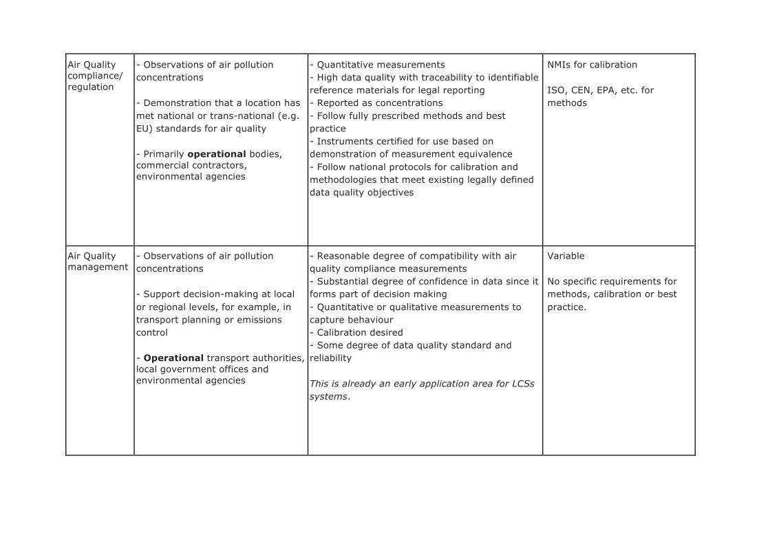
Air Quality compliance/ regulation

- Observations of air pollution concentrations - Demonstration that a location has met national or trans-national (e.g. EU) standards for air quality - Primarily operational bodies, commercial contractors, environmental agencies

- Quantitative measurements - High data quality with traceability to identifiable reference materials for legal reporting - Reported as concentrations - Follow fully prescribed methods and best practice - Instruments certified for use based on demonstration of measurement equivalence - Follow national protocols for calibration and methodologies that meet existing legally defined data quality objectives

NMIs for calibration ISO, CEN, EPA, etc. for methods

Air Quality management

- Observations of air pollution concentrations - Support decision-making at local or regional levels, for example, in transport planning or emissions control - Operational transport authorities, local government offices and environmental agencies

- Reasonable degree of compatibility with air quality compliance measurements - Substantial degree of confidence in data since it forms part of decision making - Quantitative or qualitative measurements to capture behaviour - Calibration desired - Some degree of data quality standard and reliability This is already an early application area for LCSs systems.

Variable No specific requirements for methods, calibration or best practice.

Public Information

- Observations of air pollution parameters - Support public information and awareness, citizen science activities, education, provide data for advocacy and local empowerment - e.g. operational bodies, NGOs, businesses or private individuals

- Quantitative or qualitative measurements - Flexibility in reported units - Indicative - Methods not legally prescribed, but should avoid conflict with air quality data generated from compliance/regulatory applications Already identified as a class of applications for LCS systems.

Not yet defined, although cannot diverge significantly from air quality compliance.

Proxy for exposure

- Alternative exposure measurements that can be compared to official data, or in lack of official data, can provide some order of magnitude of the exposure of a population in specific areas or buildings. - Observations of personal exposure to air pollution - Assess the human health impacts of air pollution - e.g. academic researchers, operational agencies, public health officials

- Quantitative measurements - Measurement equivalence to regulatory observations generally preferred, but not required or always possible - To support health/medical decision-making data quality requirements would become demanding An emerging application where LCSs are already displacing passive exposure sampling, particularly for PM.

Limited currently to research and occupational health. Peer-review for methods acceptance National/Trans-national occupational health-approved regulatory devices

*NMIs: National Metrology Institutes; EURAMET: European Association of Metrology Institutes; ISO: International Organization for Standardization; UNFCCC: United Nations Framework Convention on Climate Change, NOAA: National Oceanographic and Atmospheric Administration; CEN: European Committee for Standardization; GCOS: Global Climate Observing System

19. Low-cost sensors and their application in the atmospheric sciences therefore need to be considered not only in terms of the technical performance of individual devices but also in terms of the hardware, software, and data analysis frameworks that can successfully support their use for specific kinds of tasks. The kind of services that may be enabled by LCSs are only now emerging conceptually and in trial experiments and so it is inevitable that the supporting infrastructure (e.g. data quality approaches, calibration, maintenance and so on) will take time to develop around the new applications as consensus is reached on best practice.

20. For academic users of low-cost sensors it would be

expected that the overarching data quality framework associated with peer-review will persist well into the future. For those interested in using such devices for ‘new science’ the responsibility will be placed largely on users to demonstrate that data meets an appropriate quality threshold in their publications. Over time the need to demonstrate this may diminish as methods and sensors become accepted and others repeat and confirm sensor and sensor system performance.

21. For operational users making measurements that must meet some predetermined

standard of data quality, whether legally defined or through participation in some broader international activity, the existing framework (based around reference instruments) for data quality assurance will likely apply initially. Many existing atmospheric applications (for example regulatory compliance, long-term global change) have well-established requirements in terms of data quality for particular parameters, and it is unlikely that performance requirements will be relaxed. It is essential for these types of high precision applications that low-cost sensors are considered in terms of what complementary information they might bring, rather than whether they are a like-for-like replacement, just at lower purchase cost to the user.

22. The most interesting space for new thinking is for future users of LCS who may be trying to achieve new insight with atmospheric composition data, e.g. for applications such as city air pollution management or public information, where sensor system data requirements have yet to be firmly established and methods of exploiting sensor data are only in their infancy. In parallel, the users of low-cost sensors may well expand to include NGOs, campaigning and advocacy groups or individuals. These users may not necessarily be experienced in measurement science, air quality monitoring, or indeed data interpretation. These new non-expert user-led applications may

particularly benefit from the development over time of targeted guidance and support frameworks, as currently exist for research and operational users.

Low-cost sensors and their application in the atmospheric sciences need to be considered not only in terms of the technical performance of individual devices but also in terms of the supporting framework that can successfully support their use for specific kinds of tasks.

The most interesting space for new thinking is for future users of LCS who may be trying to achieve new things with atmospheric composition data.

1.4 Summary of areas to be covered in later sections 23. The report aims to cover four broad areas relating to the application and use of

low-cost sensors drawing primarily from the peer-reviewed literature available at the end of 2017. It aims to:

● Provide a view of the current state of the art in terms of accuracy, reliability

and reproducibility of a range of different sensor approaches when compared to reference instruments. It will highlight some of the key analytical principles and what has been learned so far about atmospheric low-cost sensors from both laboratory studies and real-world tests.

● Provide a summary of concepts on how sensors and reference instruments may be used together in a complementary way, to improve data quality and generate additional insight into pollution behaviour.

● Identify some applications where new scientific and technical insight may potentially be gained from using a network of sensors when compared to sparsely located observations.

● Provide advice on key considerations when matching a project/study/application with an appropriate sensor monitoring strategy, and the wider application-specific requirements for calibration and data quality.

2. MAIN PRINCIPLES AND COMPONENTS

24. Low-cost sensor systems (see example in Figure 2) contain a number of common components in addition to the basic sensing/analytical element that is used for detection. Additional components within a sensor system may include hardware for signal amplification, analogue to digital conversion, signal processing, environmental controls, power handling, batteries, physical enclosure and software components for data processing, data storage, telecommunications (e.g. WiFi, GSM, GPSRC, 3/4G, LPWAN) and visualization. These are ancillary technical components in a sensor system that assist with data processing, user convenience and usability, or support the use of a sensor as a stand-alone instrument. Many commercial sensor systems combine multiple air pollutant sensors in one system and often include sensors for non-pollutant parameters such as humidity or temperature. For those considering using LCS, it is generally the cost of the sensor system that is most relevant to users (see definitions 1.2).

Common core components and functions may include:

● The sensing element or detector ● Sampling capability, e.g. pump or passive inlet ● Power systems, including batteries and voltage/power stabilisation ● Sensor signal processing ● Local data storage ● Data transmission capability (WiFi, GPRS, 3/4G etc) ● Server-side software for data treatment ● Housing and weatherproofing

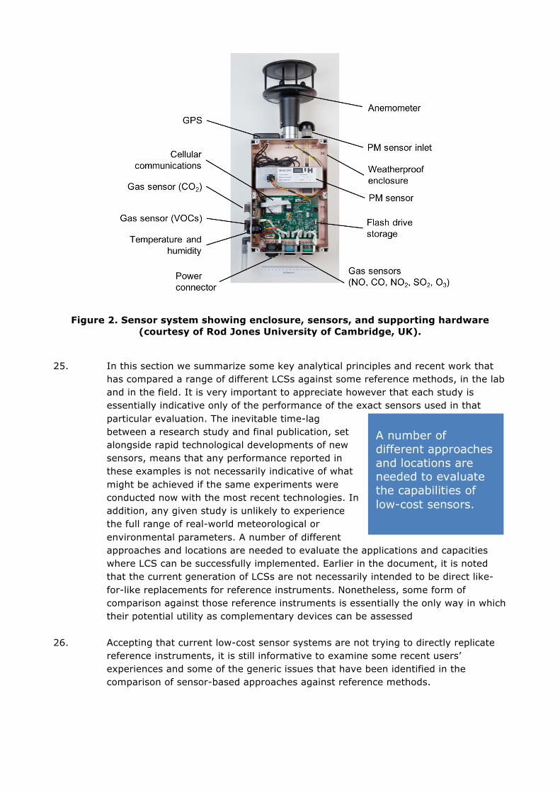
Figure 2. Sensor system showing enclosure, sensors, and supporting hardware (courtesy of Rod Jones University of Cambridge, UK).

25. In this section we summarize some key analytical principles and recent work that

has compared a range of different LCSs against some reference methods, in the lab and in the field. It is very important to appreciate however that each study is essentially indicative only of the performance of the exact sensors used in that particular evaluation. The inevitable time-lag between a research study and final publication, set alongside rapid technological developments of new sensors, means that any performance reported in these examples is not necessarily indicative of what might be achieved if the same experiments were conducted now with the most recent technologies. In addition, any given study is unlikely to experience the full range of real-world meteorological or environmental parameters. A number of different approaches and locations are needed to evaluate the applications and capacities where LCS can be successfully implemented. Earlier in the document, it is noted that the current generation of LCSs are not necessarily intended to be direct like-for-like replacements for reference instruments. Nonetheless, some form of comparison against those reference instruments is essentially the only way in which their potential utility as complementary devices can be assessed

26. Accepting that current low-cost sensor systems are not trying to directly replicate

reference instruments, it is still informative to examine some recent users’ experiences and some of the generic issues that have been identified in the comparison of sensor-based approaches against reference methods.

A number of different approaches and locations are needed to evaluate the capabilities of low-cost sensors.

3. SENSOR PERFORMANCE 3.1 Low-cost sensors for gaseous air pollutants 27. The gaseous air pollutants that are most typically measured using sensors are

nitrogen monoxide (NO), nitrogen dioxide (NO2), ozone (O3), sulphur dioxide (SO2), carbon monoxide (CO), and to a more limited extent, total volatile organic compounds (VOCs). These gases are important because of their direct and/or indirect adverse health and ecosystem effects or for their role as O3 precursor species. NO2, O3 and CO are known to be directly harmful to health as are some individual VOCs (e.g. benzene, formaldehyde, 1,3 butadiene). These species have regulatory limit or target values for their concentrations in ambient air in many countries. Other gaseous air pollutants (other VOCs, NO etc.) are important because they are precursors to the formation of secondary pollutants such as O3 in the ambient air. Measurements of the gaseous pollutants are typically reported either as a mixing ratio (e.g. ppm or ppb), or in mass concentration units (e.g. µg m-3). It is also relevant to note that sensor performance, e.g. sensitivity and measurement error might be different not only between sensors but also between pollutants measured by the same sensor.

28. In general air pollutants/reactive gases are detected using either electrochemical

(EC) sensors, metal-oxide semiconductor (MOS) sensors, or miniature photoionization detectors (PIDs). For a literature review of the subject area, see Baron and Saffell (2017).

29. In electrochemical (EC) sensors, a gaseous pollutant undergoes an electrochemical

reaction that results in a signal - manifested as a current - which is related to the concentration of the target gas in the air. EC sensors are available for a variety of gases which vary in their accuracy and reliability depending on the species being measured (see summary of literature for further results). In addition, EC sensors have been shown to have interferences with relative humidity and temperature, requiring additional measurements to be made in order to obtain reliable results (e.g. (Aleixandre and Gerboles, 2012a; Castell et al., 2017; Cross et al., 2017a).

30. Metal oxide sensors (MOS) have an exposed surface film onto which a target gas

adsorbs, a process which then results in a change in conductivity or resistance of the film itself. The small change in conductivity/resistance is measured and corresponds to the concentration of the gas at the surface. This relationship is in general non-linear in nature and these sensors have some sensitivity to changing environmental conditions, and interferences from other gases that may be present (e.g. (Fine et al., 2010; Peterson et al., 2017; Rai et al., 2017; Wetchakun et al., 2011).

31. Photo-ionisation detectors (PID) are commonly used in LCS applications and work

by using ultraviolet light to break organic molecules apart; as they are ionized, a small current is induced and is measured by the sensor. The PID lamps have specific photon energy levels and the compounds that have similar or lower ionization energies can be ionized and detected. PID has some limitations because it does not ionize VOCs with equal efficiency across different compounds; some compounds are efficiently ionized (and detected) while other compounds are less

efficiently ionized (and less efficiently detected). As a result, PID-based sensors give values for total ambient VOC that are influenced by the actual VOC mixture itself.

32. There are numerous studies that report laboratory calibrations of different sensor

types and evaluation experiments that aim to quantify a specific sensor’s sensitivity towards target gases. Experiments can test sensors under a wide range of different conditions and it is important to extract from reviews and papers the extent to which comparisons against reference instruments have been made under controlled conditions vs field conditions (knowing also that field conditions can change for a specific site), and whether other parameters such as temperature and humidity, and the concentrations of other pollutants have been allowed to vary.

33. A general consensus that has emerged over the past

ten years is that laboratory-based sensor calibrations performed under controlled lab conditions tend to produce better analytical agreements between sensors and reference instruments than is achieved when side by side comparisons are performed against naturally varying atmospheric composition in the field. In-field comparisons of gas phase sensors are widely considered as the most direct and appropriate method for comparing different measurement approaches, though it is uncertain whether sensor performance will differ when used in a different location.

34. A number of studies report differences in how a particular sensor performs between

laboratory test conditions and when the sensor is applied in ambient air (Castell et al., 2017; Jerrett et al., 2017; Lewis et al., 2015; Mead et al., 2013; Spinelle et al., 2017b) and that each sensor type can have specific sensitivities towards the target compound and other interferences. It should be noted that in this regard sensors are actually no different from many reference instruments. They too often have different characteristics when calibrated in the lab with synthetic materials compared to responses in real ambient air.

35. Numerous evaluations have used co-location alongside reference instruments as a

means to evaluate performance. Many cities have Air Quality Monitoring (AQM) sites whose locations and measurement methods are well defined in local and regional regulatory frameworks. These reference measurements are typically located in climate-controlled enclosures, have trained operators, function with prescribed methods of QA/QC and provide a useful benchmark for comparison. LCS systems are typically deployed at such sites, roof mounted at similar inlet heights, but not inside the climate-controlled environment of the reference measurements. Given often limited or no climate control of the sensor system, meteorological conditions can then be a factor and some, but not all, commercial systems perform temperature and humidity corrections to improve sensor performance.

36. Some gas sensors have been seen to be susceptible to cross-sensitivities from

other environmental factors including ambient temperature, humidity and also other common atmospheric compounds. The comparison studies that have been completed over the last decade have been important in driving change in the

In-field comparisons of gas phase sensors are widely considered as the most direct and appropriate method for comparing different measurement approaches.

underlying sensors themselves, with improved devices released by manufacturers as a result. As an example, a particular generation of NO2 electrochemical sensor was found to have up to a 100% interference to ozone when used in the field (Mead et al., 2013), and that this degree of interference was dependent on the relative concentrations of the target compound and interferents (Lewis et al., 2016). In response to the field comparison results the sensor manufacturer then adapted the sensor type, reducing this effect through use of an ozone trap prior to nitrogen dioxide measurement.

37. The outdoor environment is a complex mixture of varying pollutant concentrations,

changing meteorology and physical effects which necessitates the calibration of sensor systems in the field (De Vito et al., 2009). The most common method for performance evaluation is to co-locate sensor systems alongside existing reference instruments. Comparisons are often made using regression statistics, commonly reported as an R2 value, an intercept and a slope. This type of comparison is frequently used in both the academic and commercial literature describing commercial sensor systems, and in addition to a growing number of organized independent intercomparison assessments.

38. Most studies reported in the literature focus on intercomparisons of sensor-derived

measurements of NO, NO2, CO, and O3 co-located with existing air quality monitoring sites. This is largely for pragmatic reasons in that these compounds are typically the most commonly monitored by existing measurement networks and have the most significant user interest in terms of air quality compliance with standards. Performance comparison is often defined by the correlation statistics between the reference and sensor time series, the linearity of the sensors to the compound concentrations and the variability of the sensors compared to reference. Less commonly reported are the inter-sensor statistics, and rather few studies track sensor performance on seasonal timescales and beyond.

39. For some sensor intercomparisons, it is unclear in the literature the extent to which

the comparison between sensor and reference is blinded (e.g. fully independent observations that are only compared after the event), or whether the sensor system has used the reference information at some point as training data to calibrate responses and characteristics for that particular chemical environment.

Some example comparisons to place sensor usefulness into context

//Editors note: Consider placing the following paragraphs (41-50) into separate text box)- better to put them in the table

Study result Compound References

40. Jerrett et al. 2017 reported that a particular variety of NO EC sensors performed well compared to a reference instrument in the laboratory, in chamber experiments (Mead et al., 2013)(Mead et al., 2013 atm env) and in outdoor deployment at a AQM site (Jerrett et al., 2017). Other studies have also reported that NO EC sensors displayed a high correlation with ambient measurements made by reference instruments (Castell et al., 2017; Jiao et al., 2016) (for example R2 > 0.73), although with some under-prediction of the absolute NO concentration by the sensors (Lewis et al., 2015). After post-processing the NO sensor

concentrations were the most accurate of all the sensor types used in those studies (Castell et al., 2017; Jiao et al., 2016).

41. A few studies have found that NO2 sensors followed similar temporal patterns to

co-located reference instruments monitoring ambient air, with high correlations (R2: 0.89-0.92 (Mead et al., 2013), and 0.76 (Jiao et al., 2016)). Other studies have reported that NO2 sensor performance was highly variable sometimes with very poor correlations between NO2 sensors and reference (R2 values less than 0.25: -0.063 (Jiao et al., 2016), 0.25±0.13 (Lewis et al., 2015), 0.02 (Lin et al., 2015),0.2 (Jerrett et al., 2017)). The absolute concentrations of NO2 were not matched by the reference instruments. Some studies reported that sensors over-predicted NO2 concentrations (Jerrett et al., 2017; Lewis et al., 2015), and others finding under-predictions (Mead et al., 2013; Moltchanov et al., 2014). The current state of the literature is therefore less positive for NO2 than for NO, in terms of comparability with reference measurements, but there is clearly an improving trend in performance as newer improved sensors enter testing and deployment.

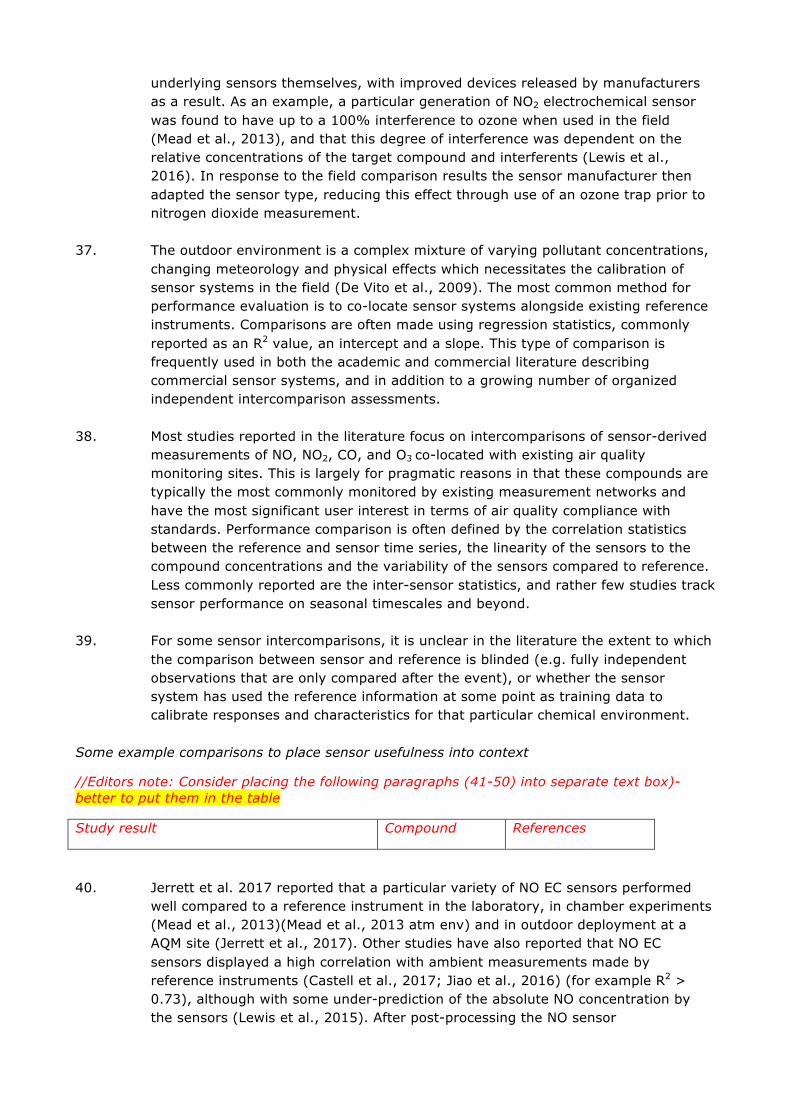
42. Lewis et al (2016) using a number of electrochemical sensors in chambers quantified a

number of NO2 cross-interferences with other atmospheric chemicals, some of which became significant at typical suburban air pollution concentrations. They highlighted that artefact signals from co-sampled pollutants such as CO2 can be greater than the electrochemical sensor signal generated by the measurand. They subsequently tested in ambient air, over a period of three weeks, twenty identical commercial sensor packages alongside standard measurements and report on the degree of agreement between references and sensors. They show that one potential solution to this problem is the application of supervised machine learning approaches such as boosted regression trees and Gaussian processes emulation. In ambient conditions they demonstrated that NO2 signal is influenced by CO2 in >40% at NO2 concentrations <30 ppb.

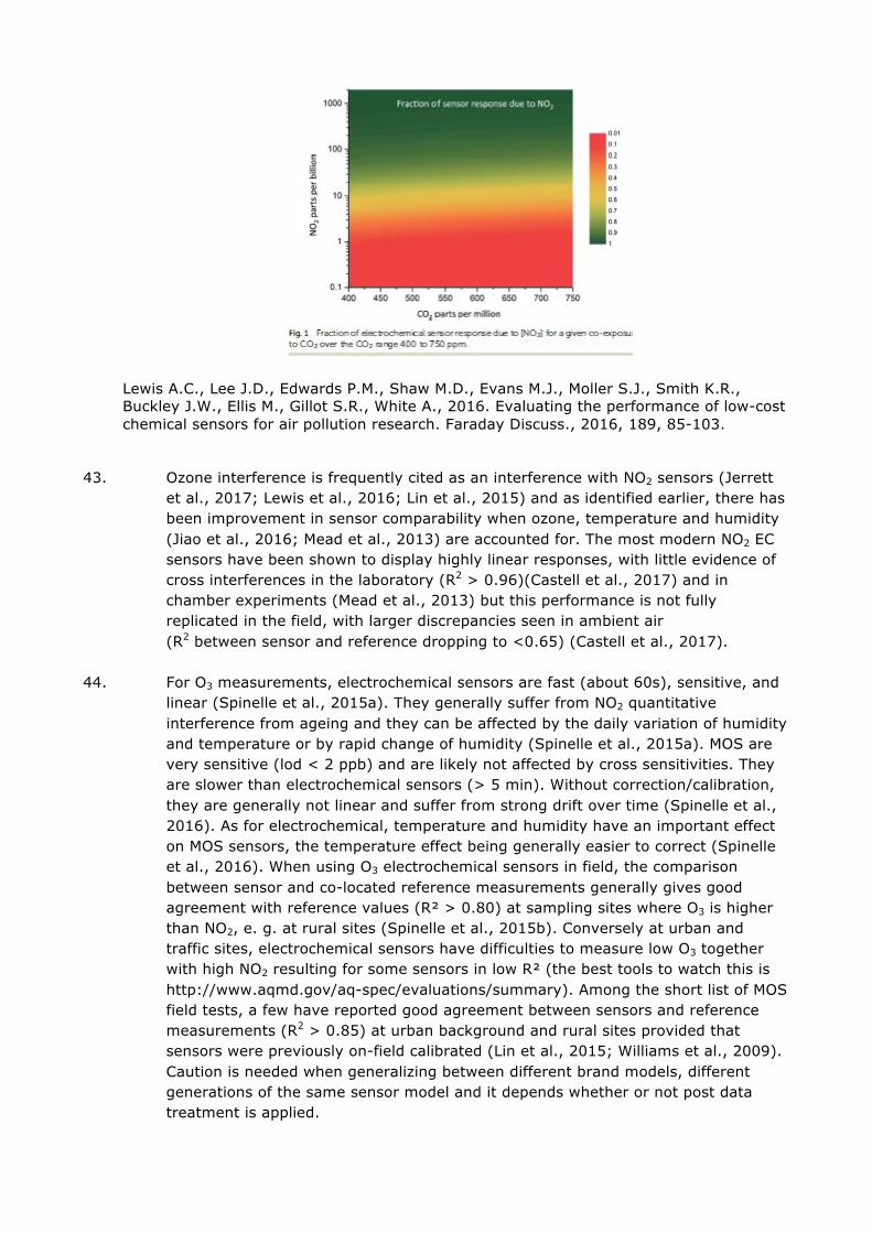
Lewis A.C., Lee J.D., Edwards P.M., Shaw M.D., Evans M.J., Moller S.J., Smith K.R., Buckley J.W., Ellis M., Gillot S.R., White A., 2016. Evaluating the performance of low-cost chemical sensors for air pollution research. Faraday Discuss., 2016, 189, 85-103.

43. Ozone interference is frequently cited as an interference with NO2 sensors (Jerrett

et al., 2017; Lewis et al., 2016; Lin et al., 2015) and as identified earlier, there has been improvement in sensor comparability when ozone, temperature and humidity (Jiao et al., 2016; Mead et al., 2013) are accounted for. The most modern NO2 EC sensors have been shown to display highly linear responses, with little evidence of cross interferences in the laboratory (R2 > 0.96)(Castell et al., 2017) and in chamber experiments (Mead et al., 2013) but this performance is not fully replicated in the field, with larger discrepancies seen in ambient air (R2 between sensor and reference dropping to <0.65) (Castell et al., 2017).

44. For O3 measurements, electrochemical sensors are fast (about 60s), sensitive, and

linear (Spinelle et al., 2015a). They generally suffer from NO2 quantitative interference from ageing and they can be affected by the daily variation of humidity and temperature or by rapid change of humidity (Spinelle et al., 2015a). MOS are very sensitive (lod < 2 ppb) and are likely not affected by cross sensitivities. They are slower than electrochemical sensors (> 5 min). Without correction/calibration, they are generally not linear and suffer from strong drift over time (Spinelle et al., 2016). As for electrochemical, temperature and humidity have an important effect on MOS sensors, the temperature effect being generally easier to correct (Spinelle et al., 2016). When using O3 electrochemical sensors in field, the comparison between sensor and co-located reference measurements generally gives good agreement with reference values (R² > 0.80) at sampling sites where O3 is higher than NO2, e. g. at rural sites (Spinelle et al., 2015b). Conversely at urban and traffic sites, electrochemical sensors have difficulties to measure low O3 together with high NO2 resulting for some sensors in low R² (the best tools to watch this is http://www.aqmd.gov/aq-spec/evaluations/summary). Among the short list of MOS field tests, a few have reported good agreement between sensors and reference measurements (R2 > 0.85) at urban background and rural sites provided that sensors were previously on-field calibrated (Lin et al., 2015; Williams et al., 2009). Caution is needed when generalizing between different brand models, different generations of the same sensor model and it depends whether or not post data treatment is applied.

45. Some electrochemical O3 sensors have been seen to under-predict absolute concentrations of O3 in controlled chamber experiments, but have presented strong correlation with reference measurements, meaning temporal patterns were accurately estimated (Castell et al., 2017). In-field ambient co-location with reference instruments has shown poorer correlation than when in the lab, but the sensors did still follow the reference instruments temporal pattern with high linearity in some cases (Jiao et al., 2016; Lewis et al., 2016). Other outdoor co-located O3 electrochemical sensors have had poorer reported correlations with the AQM reference (Jiao et al., 2016), indicating that performance can vary considerably from sensor to sensor.

46. Variability between identical sensor models is a further important characteristic to

be defined before applications can be designed. In one study (Moltchanov et al., 2014), the averaged sensor signal from a large number of MOS O3 sensors displayed a good linear relationship between the reference instrument and the sensor reported concentration, but individual sensors deviated substantially from one another. A study further using MOS O3 sensors against a reference presented a high linearity between the two types of measurements but when comparing absolute concentrations, the sensors were typically under-predicting O3 at the lowest concentrations and over-predicting the episodic ozone peaks (Lin et al., 2015).

47. Tungsten oxide (WO3) based sensors were co-located with reference instruments

outdoors at several locations (Auckland (NZ), Houston (Texas) and Raleigh (North Carolina)) to evaluate the abilities of LCSs to detect O3 in the real world, with similar results to that of several reference sites. The sensors showed a linear response to changing O3 concentrations monitored by the reference instruments although deviations between them were observed when the O3 concentration increased rapidly (Williams et al., 2013). In these studies corrections were successfully made for cross interferences, zero-air drifts and calibration for several short-term (max. four month) deployments for O3 sensors co-located with reference analysers (Williams et al., 2013).

48. The correlation between various different types of co-located CO sensors with

reference monitors has been reported to be rather variable in ambient air, sometimes with rather poor non-linear responses when deployed outdoors (R2 0.18 – 0.48) (Jerrett et al., 2017), with absolute CO sensor concentrations sometimes not matching the reference and in other studies being offset to the reference instrument. CO electrochemical instrument (Castell et al., 2017; Jerrett et al., 2017). CO sensors have showed temporal drift and some divergence of signal (Jerrett et al., 2017), but this has been shown to be consistent enough to correct for, allowing improvement in CO sensor performance and measurement comparison with reference (Jiao et al., 2016). Co-located low-cost CO MOS sensors in a further study did not follow the reference measurements at all and were non-linear (R2 = -0.4- -0.14). In the case of CO, the exact type of sensor being used is therefore critically important, since a wide range of data qualities can be experienced dependent on this.

49. Sulphur dioxide is not often measured with LCSs due to issues with limit-of-

detection in many ambient environments. In locations where there have been large-scale policy-driven mitigation efforts (United States, much of Europe) and SO2 levels have been reduced below regulated limits, LCS measurements for SO2 are

often ineffective. Studies which have been performed in such areas show little correlation to reference data (usually with SO2 < 5 ppb) (Borrego et al., 2016). However, recent literature (Hagan et al., 2018) has shown promise for using LCS’s for SO2 in environments where SO2 levels are sufficiently high which could be relevant for many countries in developing economies which still rely on high sulphur-content fuels, areas with high presence of sulphur-emitting industry, and areas near large point sources of SO2 such as volcanoes. In these instances, LCSs for SO2 have been shown to be effective when SO2 concentrations exceed 10 ppb.

50. Total volatile organic compounds are less widely monitored because reference

instrumentation is not as widely available and the alternative sensors themselves are not compound selective. Sensors provide a bulk VOC measurement whereas reference instruments give a speciated measurement (e.g. concentrations of specific organic compounds). While sensors (either MOS, or photo-ionisation detectors) can notionally report a total VOC concentration, they exhibit varying sensitivities towards different groups of VOC and this is challenging to correct for (Smith et al., 2017). MOS sensors have been co-located with a Selected Ion Flow Tube (SIFT) Mass Spectrometer (MS) indoors (a technical measurement of specific VOCs). At concentrations of 300 ppb or lower the sensors closely matched the response of the reference, but there was a high degree of non-linearity at higher concentrations. The LCSs displayed slower response times to peaks in VOC concentrations and a non-additive response when mixtures of VOC were injected, rather than individual compounds (Caron et al., 2016).

3.2 Low-cost sensors for Particulate Matter (PM)

51. Particle measurements, when categorized across different sizes are far more complex than gas measurements and depend on a variety of factors which differ for different measurement methodologies and for different particle types (chemical composition, refractive index, shape and size distribution). Particles can also be highly reactive, and reported mass concentrations are subject to sampling biases if during the process of being sampled, the particles are transferred across strong temperature/humidity gradients.

52. Low-cost PM measurement techniques most commonly rely on optical (light-scattering-based) measurements of PM, which typically use a low-power light source – either an LED or laser – where particles that are collected scatter light measured by a photo detection device. Concentration is proportional to the scattered light intensity and a particle density is usually assumed. There are two broad measurement techniques employed by LCS applications including nephelometry which measures particle light scattering of an ensemble of aerosol, and optical particle counting which measures particle size and number of individual particles. Neither technique directly measures particle mass but are usually statistically related to particle mass measured by a reference measurement

53. The size detection limit of most low-cost light scattering devices for particle number

(PN) concentration measurement can only observe particles in the ~400 nm – 10,000 nm size range, and are generally insensitive to particles outside of this range (Wang et al., 2010). This is particularly relevant if one is interested in total PN concentration such as near roadways which are usually dominated by particles less than 400 nm in diameter. There are no LCSs available that detect ultrafine particles, which are generally defined as particles less than 100nm in

diameter, since most of this light scattering systems do not detect particles with a diameter <300nm.

54. Lower limits of detection of low-cost optical particle counters are reported (Holstius

et al., 2014; Jovašević-Stojanović et al., 2015; Kumar et al., 2015) in the 1-10 µg m-3 range, though this is usually estimated under optimal laboratory conditions. Sensors have also been shown to have non-linear calibration functions with two or more response functions. They also have upper detection limits, typically in the range of 500-1000 µg m-3, making them unsuitable for extremely polluted locations. As a result, PM sensors must be calibrated against reference instruments under actual field conditions in order to derive reasonable confidence in limits of detection, accuracy, and precision.

55. PM sensors appear particularly susceptible to variable and unpredictable

performance under conditions of high relative humidity. Recent studies suggest worsening performance when relative humidity exceeds 80-85% (Crilley et al., 2018). There may also be chemical composition effects that interact with this humidity effect. That is, there may be some mixtures of aerosol that are more susceptible to relative humidity influence than others. At present, this is an emerging field of study, but it is clearly an important factor to resolve for future possible applications of PM low-cost sensors.

56. To date, there are typically few, if any, built-in QA/QC tools available in most low-

cost PM sensors to correct or adjust data. These must be deployed by a user to assess instrument performance in a field location, account for sensitivity or response drift, or to validate data during data collection. As such, long-term stability of low-cost PM sensors remains highly uncertain.

57. There are a few available devices for particle size distribution, but LCS options

generally offer relatively coarse size resolution. There are no LCS devices capable of measuring the size distribution of ultrafine particles, and these types of measurements are better assessed with traditional laboratory-based instrumentation and techniques and are not yet suitable for low-cost measurement approaches.

58. Though they are often based on similar operating

principles, a number of key differences exist between low-cost and reference optical PM instruments: (1) reference optical instruments maintain a constant relative humidity within the sampling inlet of the system (they dry particles) whereas low-cost PM sensors operate at ambient relative humidity which leads to different results depending on particle hygroscopicity; (2) reference instruments are comprised of precision optics (for focusing laser light and collecting scattered light), superior particle flow control, and highly sensitive optical detectors, the combination of which allows for much lower background noise and improved detection of smaller particles.

59. Literature does however support that: (1) low-cost approaches can be useful for qualitative assessment of concentration in a moderately polluted environment, and that; (2) deployment of many sensors on a community or neighbourhood-scale can

A number of major differences exist between low-cost and reference optical PM instruments.

provide sufficient data granularity to provide insight into spatial and/or temporal patterns and source contributions. This may be useful for refinement of modelling approaches, assessing human exposures, or producing datasets for long-term trend analysis.

3.3 Low-cost sensors - greenhouse gases 60. Greenhouse gas sensors often use miniaturised versions of optical absorption

methods that can also be found in reference instruments. This section gives an overview of common measurement methods for greenhouse gases and provides a brief overview of laboratory measurements and field projects that have compared sensor scale devices for greenhouse gases (GHGs) against reference instruments.

61. Comparatively few studies using sensors for atmospheric measurements of GHGs

are available in the literature. Most of them have utilised sensors for CO2 and only very limited number of publications were found examining sensors for CH4 (Collier-Oxandale et al., 2018; Eugster and Kling, 2012a; Suto and Inoue, 2010). For CO2, LCSs are based on non-dispersive infrared absorption (NDIR). NDIR is a technique in which infrared light is absorbed by sampled CO2, where the amount of light absorbed is proportional to concentration. The CH4 sensor in (Collier-Oxandale et al., 2018; Eugster and Kling, 2012a; Suto and Inoue, 2010) was based on a metal oxide semi-conductor as the gas sensing material.

62. Shusterman et al. (2016) presented the use of NDIR absorption sensor in each

node in a network (BEACO2N). An advantage of such techniques is that performance can to a degree be evaluated from first principles knowledge of instrument features such as path length and absorption properties of the specific gas of interest. Some low-cost greenhouse gas sensors have been shown to possess adequate sensitivity to resolve diurnal as well as seasonal phenomena relevant to urban environments (Rigby et al., 2008) and in hardware terms, have costs that are one to two orders of magnitude lower than commercial cavity ring-down instruments commonly used in global carbon tracking networks.

63. Most of the published studies using LCSs for CO2 have focused on the

characterization of the sensor performance from comparison against reference instruments under field conditions. Spinelle et al., (2017b) evaluated the performance of two types of low-cost NDIR sensors from field tests. This group used different statistical and machine learning approaches to evaluate their data and assess interfering factors such as ambient temperature and relative humidity. The best results were achieved using machine learning techniques such as Artificial Neural Networks (ANN), where sensor uncertainty was 5% in the range from 370 to 490 ppm CO2 (typical ambient concentrations) but increased up to 30% when a less sophisticated linear regression model was applied. It should also be noted that these results were only obtained with simultaneous availability of a reference instrument during the first 10% of the comparison period. This suggests that in some cases, uncertainty will be higher when using less sophisticated machine learning techniques to calibrate instruments.

64. The performance of different calibration models for the correction of a NDIR sensor

signal operating under field conditions has also been explored in the study by (Zimmerman et al., 2018). It was again found that a machine learning technique (Random Forest models) outperformed multiple linear regression models. The

absolute mean error of the CO2 sensor measurements was reported to be 10 ppm during a 16-week testing period. It should, however, be noted that the sensor performance was evaluated using training and test data measured at the same field location and that the applied calibration model included the signal of a separate CO sensor as an interfering factor. The transferability of the determined calibration model to locations with different relationships between CO2 and CO might therefore be limited.

65. A study by Kunz et al., (2017) showed that it was possible to use small and

inexpensive sensors for atmospheric measurement of CO2 with an accuracy that is sufficient for targeted applications. It seems, however, inevitable that the sensor units are individually being tested and corrected for their response to changing temperature, pressure and relative humidity (when the air sample is not dried). A reasonable way to do this is to test measurements in environmental chambers and then verify the applicability of the determined data correction parameters through comparison of the resulting sensor signal with reference instruments during field tests. This suggested procedure seems necessary but is not sufficient for typical applications of sensors. When sensors are deployed away from reference instruments, strategies for continuous quality assurance and quality control of the sensors must be implemented as outlined and applied in Kunz et al., (2017). This is of course not specific for sensors for GHGs but applies to all sensors for atmospheric gases and particles (see chapter 5).

66. In publications that have used sensors for atmospheric CH4 (Eugster and Kling,

2012b; Suto and Inoue, 2010), the sensors were found to be sensitive to ambient temperature and relative humidity. Based on measurements under field conditions in Alaska (Eugster and Kling, 2012a), it was concluded that the relative concentration derived from the sensors was sufficient for preliminary measurements needed to locate potential methane (CH4) hotspots. However, correction of the temperature and humidity cross-sensitivity was required, and the performance of these sensors does not allow for long-term studies where accurate methane measurements are needed. Removal of water vapour to less than 10 ppm as well as catalytic conversion of other flammable gases was needed for the sensor system used in Suto and Inoue (2010), in order to allow for monitoring of atmospheric methane.

67. Collier-Oxandale et al. (2018) investigated low-cost methane sensing approaches at

two different deployments, at sites near active oil and gas operations and in an urban neighbourhood subject to complex mixture of air pollution sources including oil operations. Field normalizations were used to generate calibration models for the sensors, which included co-locating the LCS systems with reference instruments for a given period. They concluded that these sensors will likely never replace traditional air quality monitoring methods, but they can provide useful supplementary information on local pollution sources. However, more research into cross-sensitivities and other deployment issues will certainly be necessary.

4. EVALUATION ACTIVITIES FOR LCSs 68. Over the past decade there have been worldwide efforts to evaluate the usefulness

and possible applications of LCS technology. Performance evaluation projects have focused on determining the quality of the data produced by sensor systems by comparing their response to reference instruments in the laboratory and in the field. Complementary to this, demonstration projects have explored how the use of these sensor systems may give new insight into atmospheric processes. There are many interested users; performance and demonstration projects have engaged governmental organizations, research groups, city departments, and community groups all seeking to understand how LCSs may be used. The following two sections provide examples illustrating some recent performance evaluation and demonstration efforts, and what lessons might be drawn from these.

4.1 Performance evaluation programmes 69. Performance evaluation programmes have been undertaken by many different

organizations, all seeking to evaluate in quantitative terms how LCSs compare against reference measurements in laboratory and ambient sampling conditions. Laboratory evaluations allow researchers to control conditions and examine the response of sensors to different temperatures, relative humidity, a range of gas or particle concentrations, and other potential interfering factors. Whereas evaluation in outdoor conditions provide a “real-world” test of the sensor systems but may be limited to the range of atmospheric conditions experienced at a particular location.

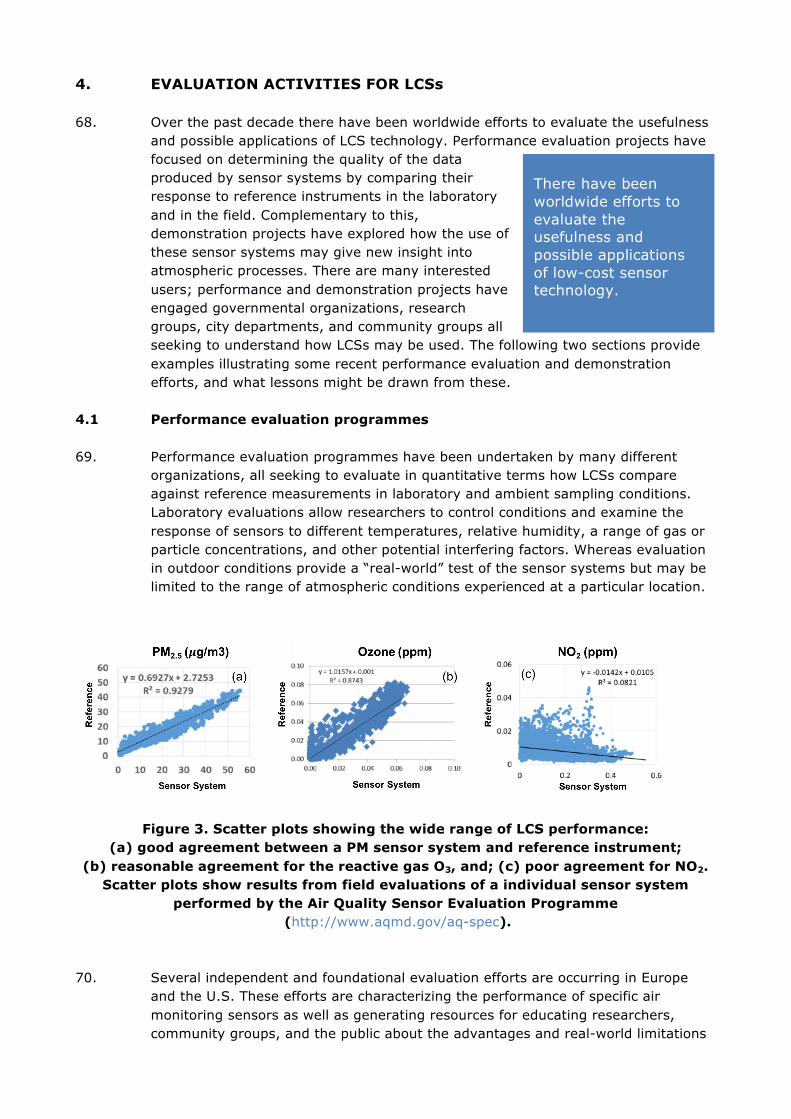
Figure 3. Scatter plots showing the wide range of LCS performance: (a) good agreement between a PM sensor system and reference instrument;

(b) reasonable agreement for the reactive gas O3, and; (c) poor agreement for NO2. Scatter plots show results from field evaluations of a individual sensor system

performed by the Air Quality Sensor Evaluation Programme (http://www.aqmd.gov/aq-spec).

70. Several independent and foundational evaluation efforts are occurring in Europe

and the U.S. These efforts are characterizing the performance of specific air monitoring sensors as well as generating resources for educating researchers, community groups, and the public about the advantages and real-world limitations

There have been worldwide efforts to evaluate the usefulness and possible applications of low-cost sensor technology.

of such sensor systems. In all cases, results from sensor analyses are manufacturer and model specific, and one should not assume all sensor models for a particular compound will perform as indicated here.

71. The Joint Research Center (JRC) has been evaluating air sensors since the late

2000s. They have a laboratory for evaluating gas sensors and have conducted many laboratory and field evaluations of sensor systems. Initial efforts focused on evaluating O3 and NO2 sensors (Aleixandre and Gerboles, 2012b; Penza et al., 2014). For O3, an evaluation of metal oxide sensors in laboratory conditions (Spinelle et al., 2016) showed slow response times, non-linear relationships with reference data, limits of detection of several ppbs, but little to no interference with other gases (NO2, NO, CO, CO2 and NH3). Longer-term (more than 6 months) evaluations however have showed that changes of temperature and humidity could generate measurement uncertainties over 100%.

72. For ozone and nitrogen dioxide electrochemical sensors, a laboratory evaluation

(Spinelle et al., 2015b) showed a good linear response, appropriate ambient limit of detection and a repeatability better than 10 ppb. When testing the interference effects of O3, NO2, NO, CO, CO2 and NH3, it was found that O3 sensors were only affected by NO2 while NO2 sensors were affected by O3 with interference in the order of 100%. The longer-term drift (more than 6 months) of electrochemical sensors was less than that seen MOS. More recently JRC evaluated performance of benzene and VOC sensors (Spinelle et al., 2017a). The conclusion was that current sensor technology was not able to accurately and selectively measure benzene at ppb ambient levels (there is a limit value of 1.5 ppb in the European Air Quality Directive). A wider conclusion was that calibration of these sensors is critical and JRC explored several calibration methods including linear regression, multiple linear regression, and artificial neural network (Spinelle et al., 2015b, 2017b). The artificial neural network was preferred and led to uncertainties of less than 20%. JRC continues to conduct a wide range of other research on sensor systems including developing a protocol for evaluating sensors (Spinelle et al., 2013) and development of open source AirSensEUR sensor platform (Kotsev et al., 2016).

73. EuNetAir Air Quality Joint Intercomparison Exercise organized in Portugal

focused on the evaluation and assessment of environmental gas, PM and meteorological microsensors, versus standard air quality reference methods through an experimental urban air quality monitoring campaign. A mobile laboratory was placed at an urban traffic location in the city centre of Aveiro to conduct continuous measurements with standard reference analysers for CO, NOx, O3, SO2, PM10, PM2.5, temperature, humidity, wind speed and direction, solar radiation and precipitation. Approximately 200 sensors were co-located at this platform. Overall, significant differences were observed across the different sensors considered. Some sensors were in good agreement with the reference, but with others substantially disagreeing. More promising results included O3 (R2: 0.12 - 0.77), CO (R2: 0.53 - 0.87), and NO2 (R2: 0.02 - 0.89). For PM (R2: 0.07 - 0.36) and SO2 (R2: 0.09 - 0.20) the results showed a poor performance with low correlation coefficients between the reference and sensor measurements (Borrego et al., 2016).

74. U.S. Environmental Protection Agency (USEPA) began evaluating air quality

sensors in 2013. Initially these efforts comprised laboratory tests of O3 and NO2 sensors and these showed: (1) very fast response times with minimal rise and lag

times which suggests potential use for continuous or near-continuous environmental monitoring; (2) a high degree of linearity over their full response range at concentrations; (3) detection limits higher than reference instrumentation; (4) cross-sensitivity interference from other gases (e.g. NO2, O3, SO2), and; (5) high relativity humidity and temperature resulted in some undesirable response characteristics (Williams et al., 2014). Later field studies of sensors measuring NOx, O3, CO, SO2, and particles revealed more variable performance when compared to reference monitors (Jiao et al., 2016). USEPA continues to conduct a wide range of sensor development, evaluation, and demonstration projects with results published on their Air Sensor Toolkit website (https://www.epa.gov/air-sensor-toolbox).

75. The South Coast Air Quality Management District (Los Angeles, USA)

started the Air Quality sensor performance evaluation center (AQ-SPEC) in 2014. The center’s goal is to provide guidance on the performance and application of sensors, promote use of sensor technology and minimize confusion with users purchasing and using new LCSs. The pollutants covered included the key EPA criteria pollutants and some air toxics. The AQ-SPEC programme has provided a method to evaluate the performance of a range of different devices and sensor data. Work involved both laboratory and field testing. A number of reports (~30) from field tests appear on the AQ-SPEC website (http://www.aqmd.gov/aq-spec/evaluations/field). Field evaluations generally indicated performance of CO, NO, O3 sensors was good, a number of oxidant sensor (e.g. O3/NO2) measurements were problematic (due to interferences), and SO2, H2S & VOC measurements were not in strong agreement at this location. PM2.5 sensors had in general a high correlation with EPA-approved instruments, but PM10 was problematic and it was noted that continuous sensor calibration was needed; very small particles (0.5 µm) were not detected at all and conversion between mass and particle numbers was not straightforward.

4.2 Low-cost sensor demonstration projects

76. The prior section referred to various efforts to quantify the performances of sensors

by evaluating them in the laboratory or under field conditions. Rapid product development, low-cost, and relative ease-of-use is resulting in deployment of distributed networks to demonstrate the value and usefulness of sensor systems. Such experiments do not aim to provide precise side-by-side comparison data but instead show how a sensor-based approach may give additional insight into atmospheric composition. Demonstration projects have engaged both traditional users and new communities unfamiliar with traditional air monitoring. Newer users are often interested in using sensor networks to understand local air quality conditions, identify local sources, implement educational/outreach programmes, and identify appropriate mitigation strategies where applicable.

77. Citizen science initiatives have been particularly

significant in demonstration projects; some projects have been in partnership with traditional research institutions (universities, governmental agencies,

LCS represent a clear opportunity through citizen science initiatives in expanding the ability to make new measurements in low and middle income countries which are often understudied by the research and operational atmospheric science communities.

industry) while others have been managed entirely by private sector groups or individuals interested in air quality. LCS represent a clear opportunity through citizen science initiatives, expanding the ability to make new measurements in low and middle-income countries which are often understudied by the public health and atmospheric science research communities.

78. Though the intent of most citizen-science projects is to gain insight into questions

of local air quality, it is often not possible for external audiences to fully discern the quality of the data collected. To date, the evidence collected is most useful in understanding the logistical features of citizen science itself, including salient issues of pragmatism, such as whether it is possible to recruit willing participants, and assessing the types of questions that communities wish to address. Some of these projects include United Nations Development Programme, Ministry of Data Balkans Green Machine Team, the CityOS project in Sarajevo, Bosnia & Herzegovina, and the Air pollution Interdisciplinary Research (AIR) Network in Kenya.

79. There are however a number of demonstration projects using sensors that include

experienced users and research organizations where insight into both process of sensor use and more quantitative outcomes can be obtained. An example is the BEACO2N project in Northern California (Kim et al., 2017; Shusterman et al., 2016; Turner et al., 2016) which is a multi-pollutant sensor project using a distributed network of approximately 50 sensor “nodes”, each measuring CO2, CO, NO, NO2, O3 and particle matter at 10 second time resolution at approximately 2km spacing in locations surrounding the San Francisco Bay Area.

80. The preliminary analysis of the first three years of CO2 observations provided

evidence of the expected diurnal and seasonal cycles as well as an encouraging sensitivity to short-term changes associated with local emission events. Further work is needed to fully assess the efficacy of inverse methods based on the BEACO2N approach, however it constitutes a promising infrastructure upon which further advances in high-density atmospheric monitoring can be built. The network has also provided insight into calibration models for CO, NO, NO2, and O3 that make use of multiple co-located sensors, a priori knowledge about the chemistry of NO, NO2, and O3, as well as an estimate of mean emission factors for CO and the global background of CO.

81. The Zurich O3 & NO2 network (Mueller et al., 2017) was a blended network of

LCSs co-located nearby to a regulatory network of standard reference air pollution monitors in Zurich. O3 and NO2 low-cost gas sensors were shown to provide concentration measurements with an accuracy of a few ppb in the first 1-3 months of operation. Comparisons with diffusion tube measurements and measurements from AQM sites revealed that this accuracy could not be maintained during the entire 1-year network deployment due to the changing response behaviour of the sensors. Several issues were encountered that were related to the employed sensors that affect a temporary (∼ hours) or persistent decrease of sensor accuracy. Hence, the application of performance monitoring strategies is a prerequisite of operating LCSs with such properties in order to be able to assess the quality of the data.

82. All the sensors in this network required individual calibration. Sensor calibration

next to reference sites was seen to be time consuming and required infrastructure. Moreover, the quality of the compiled calibration data set for the model parameter

estimation depended on the prevalent ambient conditions (i.e. encountered pollutant concentrations, meteorology). The signal of the NO2 sensors was heavily impacted by changes in relative humidity. This effect could be reduced to a certain degree by the application of a correction function but still limited the achievable accuracy of the sensors. This issue points to the necessity of an improved mathematical description of the sensor based on its working principle in order to describe sensor behaviour in more detail. More sophisticated sensor models may facilitate calibration as its parameters could be constrained with less effort than is required when applying regression models.

83. NO2 and O3 concentration predictions could be derived at the level of a few ppb at

specific time periods for many locations in Zurich using the data from the AQM network which covered a wide range of different pollutant situations. This feature can be a substantial factor for an effective monitoring of the sensor performance in LCS networks. Moreover, such data can be used for the remote correction of sensors. In this study this procedure was shown to improve the results of NO2 sensors.

84. The Hong Kong Green Marathon sensor network (Sun et al., 2016) was an ad

hoc sensor-based air quality monitoring network with 6 sets of sensor systems deployed along the marathon route, including electrochemical based NO2, CO, O3 and photometer based PM2.5 measurements. Real-time monitored air pollution concentration data were transmitted back to the server centre with Air Quality Health Index (AQHI) calculated on an hourly basis. Intensive quality assurance and quality control measures were conducted for sensor calibration and data quality control. High linearity of sensor response to the pollutants in the laboratory was observed. Due to the short deployment period, a relatively narrow variation of temperature and relative humidity conditions during the field test made it favourable to use simplified sensor equations with good performance when comparing to side by side reference data in AQM stations. High correlation coefficients (>0.96) were all observed for NO2, CO and PM2.5 between the sensor systems and the reference instruments. The air sensor network data from the roadside of a busy main road during and after the marathon event showed the effectiveness of temporary traffic control on creating a significant reduction of concentrations of traffic-related air pollutants, such as NO2 and CO. According to the tunnel sensor node, mechanical ventilation demonstrated a substantial impact on improving the air quality.

85. The Location Aware Sensing System (LASS) project in Taiwan currently has

more than 5000 devices deployed in 36 countries. This network includes low-cost PM2.5 sensing devices (USD 100-500) from commercial products, internet maker groups, and scientist research groups, with 2 or 3 different PM2.5 sensor components (Chen et al., 2017). This network is evolving rapidly as a collaboration among research groups, governmental agencies, NGOs, and commercial companies, including efforts by citizen scientist ‘Makers’. The data is displayed in a near real-time with several options of visualization (https://airmap.g0v.asper.tw/) and the data portal is maintained by Academia Sinica (https://pm25.lass-net.org/en/). Roughly 100 of these sensor devices have been calibrated in the laboratory and the field against reference instruments, with reported correlation coefficients exceeding 0.80. Different calibration curves are needed for different concentration ranges such as <30, 30-150, and >150 ug/m3, and sensor precision is reported to within 20% variability. An anomaly detection framework for

large-scale PM2.5 sensing systems is used to detect sensor malfunction and spatio-temporal anomalies has been proposed using data analytics (Chen et al., 2018). The following scientific challenges and opportunities arise: (1) this network is comprised of PM2.5 sensor components with different stability, variability, and sensing frequency; (2) the vast number of the devices require big data analytics to make sense of the measurements; (3) the network has potential applications in different research fields with participatory approaches; and (4) the network can potentially be used in validation and development of fine-resolution air pollution transport and dispersion models.

86. An Italian national project RES-NOVAE - Networks, Buildings, Streets: New

Challenging Targets for Environment and Energy deployed one mobile and 10 stationary nodes which were installed in specific sites (buildings, offices, schools, streets, port, airport) to enhance citizen’s environmental awareness. Continuous measurements were performed by low-cost electrochemical gas sensors (CO, NO2, O3, SO2), an optical particle counter (PM1.0, PM2.5, PM10), an NDIR infrared sensor (CO2), and a photo-ionisation detection (total VOCs), including microsensors for temperature and relative humidity. As an example, the Mean Absolute Error (MAE) of PM10 for three reported nodes is equal to 5.6 µg/m3, while the accuracy ranges from 24.8% (Node 1), 21.6% (Node 2) to 20.5% (Node 6). Moreover, for sensor-node 6 (airport), a good correlation coefficient (R2 = 0.80) for PM10 and a high classification coefficient (C = 70%) have been measured for AQI compared to a measurement by a reference instrument (Penza et al., 2017).

87. Many other projects for sensor networks are planned around the world, and Annex

1 records a number of these for the readers reference alongside the recommendations for further reading. The rate of change in the field is so rapid that this list is inevitably out of date but it provides a range of links to other sensor based projects that can be tracked for their outputs over the coming years.

88. In summary, larger multi-node sensor networks based on LCSs have already

emerged as test projects in a number of locations around the world. The most important area of uncertainty from the current round of demonstration studies is how to most effectively utilize these new measurements given that there are known issues regarding data quality and the stability of responses over time. Care should be taken in understanding the exact intent of demonstration studies, particularly to determine whether networks were designed to test a network’s ability to quantify air quality or greenhouse gases, or whether the network was to test the feasibility, citizen engagement or wider issues associated with deploying a sensor network.

5. CALIBRATION AND QUALITY ASSURANCE/QUALITY CONTROL OF

LCSs 89. There are a wide range of users of LCS devices, and the user (and application) will

dictate the necessary level of data quality. For example, devices positioned as hobby/consumer products will have lower expectations than those used for operational air pollution management or controls. LCS challenge the status quo and therefore may need adoption of new and different approaches for QA/QC to those currently used for the measurement of air pollution and greenhouse gases.

90. While various stakeholders will have different requirements for accuracy and traceability, it is imperative that there is a transparent characterization of how a given sensor behaves – after all, “data of poor or unknown quality is less useful than no data since it can lead to wrong decisions” (Snyder et al., 2013). To address this issue, there is a critical need to establish a cohesive approach for the evaluation and performance assessment of LCSs prior to their large-scale adoption in atmospheric science (Lewis and Edwards, 2016).

91. That being said, air pollution sensors should be treated as any other analytical

instrument; they will likely require regular calibration and will show long-term changes in drift and sensitivity. For the purpose of this document, we define a calibration of a LCS as the establishment of a relationship between the output of a LCS and a measurement standard, where a measurement standard in this context can be either a calibrated reference instrument or gas/particle standard.

5.1 Calibration and Quality Assurance

92. The calibration of LCSs involves determining the model used to convert between the measured parameter (e.g. light absorption, voltage, or conductivity) and desired output variable (e.g. pollutant/species concentration). Typically, this is fairly transparent, with these factory calibration settings published in component data sheets, and at present, it is likely many users rely on these factory calibration settings. However, there is little evidence to suggest, at least for the current generation of LCSs, this is sufficient to provide accurate, reliable data across various environments in which the sensor may be used. To determine whether or not a factory calibration is sufficient, a validation (quality assurance) of the data should be performed in an environment similar to the one in which the LCS will be used.

93. Currently, there are two main approaches to calibrating LCSs: laboratory calibration

and field co-location; both methods have benefits and drawbacks. 94. Laboratory calibration typically involves the same process used to calibrate

reference and research-grade analytical chemistry instruments: subjecting the sensor to a series of known concentrations of pollutant/species using known measurement standards in a controlled environment. This approach has been explored extensively in the literature (Castell et al., 2017; Mead et al., 2013; Piedrahita et al., 2014); unfortunately, the conditions under which sensors are calibrated in the laboratory do not often overlap with the full range of conditions encountered in an ambient environment. These differences include the presence of cross-sensitive gaseous species (Lewis et al., 2016), changes in relative humidity and temperature, and ever-evolving aerosol physical and optical properties, all of which are known sources of error for LCS measurements. Laboratory experiments are also limited to those with the resources and/or opportunity to access the necessary equipment, which may not be available to all stakeholders. However, laboratory experiments can be very useful for determining how LCSs behave under very specific, controlled conditions which contribute to our fundamental understanding of how they work. If using a laboratory calibration as a primary

“Data of poor or unknown quality is less useful than no data since it can lead to wrong decisions” (Snyder et al., 2013).

calibration approach, it is important to mimic the deployment environment of the sensors as closely as possible (e.g. using an environmental chamber to scan the typical range of temperature, humidity, pressure, etc.).

95. To overcome some of the limitations encountered in the laboratory, many have

found ambient co-location calibrations to be most effective. Here, the sensor (or sensors) is placed in the field near a reference instrument for a period of time to provide a direct comparison of the LCSs output to that of a calibrated reference instrument. Unfortunately it is quite difficult to observe the entire dynamic range of target species, cross sensitive species/pollutants and environmental parameters in a short period of time and this which may make comprehensive calibrations rather time intensive. Access to locations and calibrated reference equipment can also be an issue. The seasonal change of the field environmental conditions should be considered (in addition to the LCS drift) to determine the frequency of the field co-location calibration.

96. When planning and performing a calibration of a

LCS, important factors to consider are temperature, relative humidity, and cross-sensitive gas species (details can be found often in data sheets and in literature) for gas-phase sensors, and relative humidity, composition, size distribution, and optical properties for particle sensors. AS was described in earlier sections, PM measurements using LCS are essentially experimental in nature and do not map easily only reference data; more research and experimentation into performance compared against calibrated reference monitors is needed.

97. For both approaches mentioned above, an active

area of research is determining the optimal algorithm used to convert raw sensor data (often current or voltage for gas-sensors, histogram or raw counts for particle sensors) into a usable format (concentration, mixing ratio, aerosol loading). Many have used variations of a parametric regression with some success (Jiao et al., 2016; Lewis et al., 2016; Masson et al., 2015; Mueller et al., 2017; Popoola et al., 2016; Sadighi et al., 2017; Smith et al., 2017) though many nonparametric/machine-learning approaches have appeared recently in the literature (Cross et al., 2017b; Hagan et al., 2018; Spinelle et al., 2015b; Zimmerman et al., 2018) as they can account for environmental effects and interference with cross-sensitive species.

Important factors to consider are temperature, relative humidity, and cross-sensitive gas species (can be found in data sheets and in literature) for gas-phase sensors, and relative humidity, composition, size distribution, and optical properties for particle sensors.

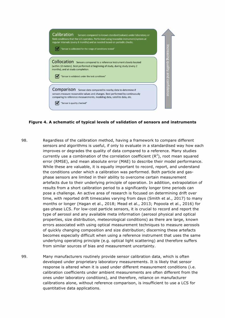
Figure 4. A schematic of typical levels of validation of sensors and instruments

98. Regardless of the calibration method, having a framework to compare different sensors and algorithms is useful, if only to evaluate in a standardised way how each improves or degrades the quality of data compared to a reference. Many studies currently use a combination of the correlation coefficient (R2), root mean squared error (RMSE), and mean absolute error (MAE) to describe their model performance. While these are valuable, it is equally important to record, report, and understand the conditions under which a calibration was performed. Both particle and gas-phase sensors are limited in their ability to overcome certain measurement artefacts due to their underlying principle of operation. In addition, extrapolation of results from a short calibration period to a significantly longer time periods can pose a challenge. An active area of research is focused on determining drift over time, with reported drift timescales varying from days (Smith et al., 2017) to many months or longer (Hagan et al., 2018; Mead et al., 2013; Popoola et al., 2016) for gas-phase LCS. For low-cost particle sensors, it is crucial to record and report the type of aerosol and any available meta information (aerosol physical and optical properties, size distribution, meteorological conditions) as there are large, known errors associated with using optical measurement techniques to measure aerosols of quickly changing composition and size distribution; discerning these artefacts becomes especially difficult when using a reference instrument that uses the same underlying operating principle (e.g. optical light scattering) and therefore suffers from similar sources of bias and measurement uncertainty.

99. Many manufacturers routinely provide sensor calibration data, which is often

developed under proprietary laboratory measurements. It is likely that sensor response is altered when it is used under different measurement conditions (i.e. calibration coefficients under ambient measurements are often different from the ones under laboratory conditions), and therefore, reliance on manufacturer calibrations alone, without reference comparison, is insufficient to use a LCS for quantitative data applications.

5.2 Quality Control of Sensors and Sensor Networks

100. Quality control is the act of monitoring the long-term performance of a LCS during deployment in a sensor network to ensure it remains in calibration, and can help notify the appropriate party when a LCS needs to be corrected or removed and undergo re-calibration, likely when the bias exceeds the measurement uncertainty. Like their reference instrument counterparts, LCSs have a limited service lifetime, but this has yet to be determined for many LCSs, and can depend greatly on the environment in which a LCS is deployed (e.g. high pollution environments can cause PM sensors to foul, low humidity environments can cause sensitivity decay in electrochemical gas sensors). Quality control is ultimately the method for determining end-of-life for a sensor. A user should apply quality control statistics to define the end-of-life for LCSs if using them over a sufficiently long period of time.

101. There are several parameters that should be

monitored over time including baseline drift (change in intercept) and changes in sensitivity (e.g. changes in slope). If these values are known or can be calculated, data can be corrected over time with data post-processing (data correction). Several approaches to quality control have been proposed in literature. One approach is to periodically compare the values obtained with a LCS to a nearby (but not co-located) reference monitor (Mueller et al., 2017). In some locations, especially those throughout Europe and the United States, reference data is made available by regulatory agencies and can be accessed either through their websites or via public groups such as OpenAQ (https://www.openaq.org). However, it is important to be aware of possible limitations with this approach, since the concentrations of some reactive gaseous species (e.g. NO, NO2, CO, O3) may be significantly different, even over modest spatial lengths (100’s of meters).

102. A second approach that has recently appeared in the literature, is to use knowledge

of regional atmospheric chemistry in combination with a small number of anchor points (reference stations) to perform remote calibrations (Kim et al., 2017). Similarly, statistics-driven quality control checks based on transport phenomena could provide information on relative differences amongst sensors within a localized network.

103. While these approaches are under active development, they do appear to be

promising methods that may could save time and effort in supporting quality checks on large numbers of sensors, especially as sensor networks move from tens of sensors to thousands of sensors. Regardless, this is an active area of where more research activity is encouraged.

104. Moving forward, as public interest in the utility of sensor networks continues to

grow, it will be important to develop and refine new calibration and quality control approaches that allow users to better understand the quantitative capabilities of their sensors. Refining both the techniques used as well as the ways in which researchers, industry, and stakeholders validate the performance of networks is

There are several parameters that should be monitored over time including baseline drift (change in intercept) and changes in sensitivity (e.g. changes in slope).

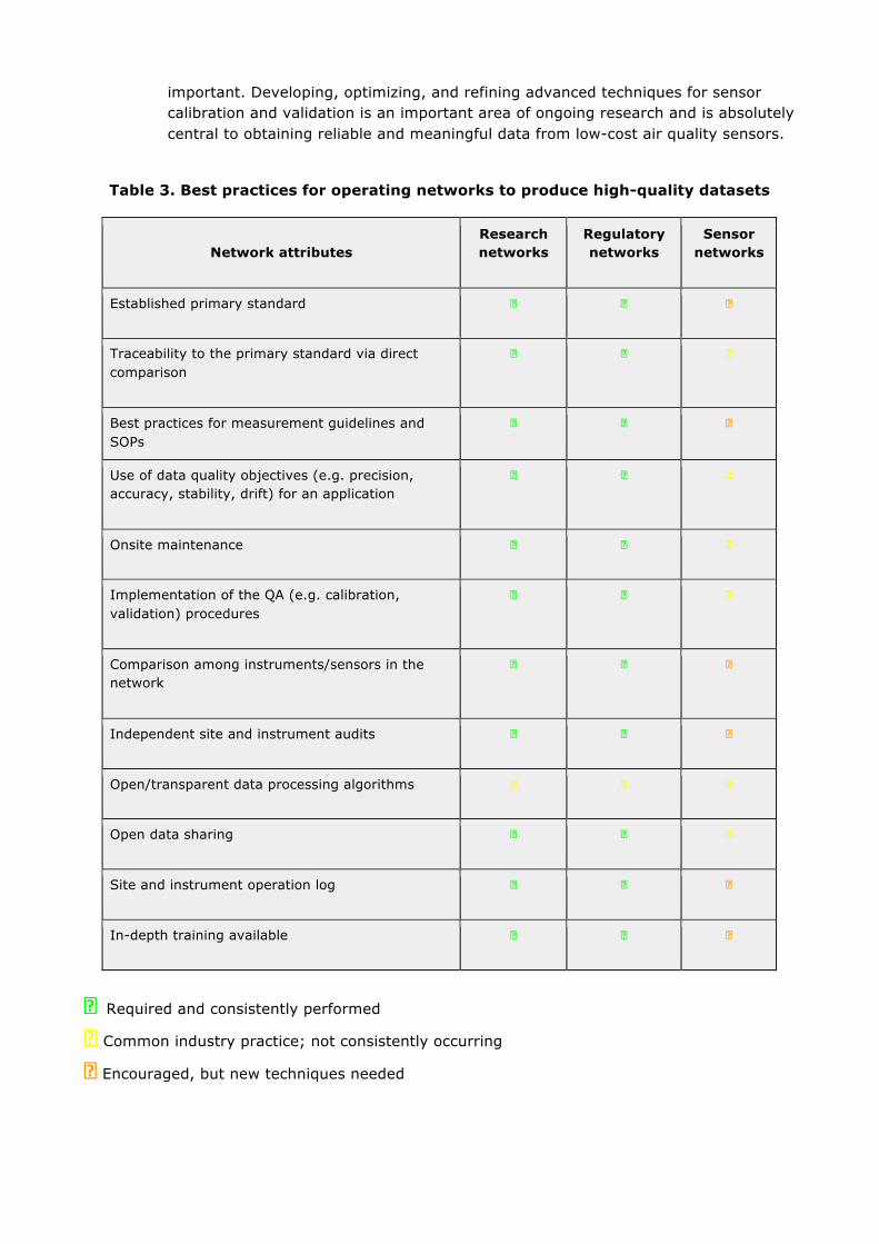
important. Developing, optimizing, and refining advanced techniques for sensor calibration and validation is an important area of ongoing research and is absolutely central to obtaining reliable and meaningful data from low-cost air quality sensors.

Table 3. Best practices for operating networks to produce high-quality datasets

Network attributes

Research networks

Regulatory networks

Sensor networks

Established primary standard � � �

Traceability to the primary standard via direct comparison

� � �

Best practices for measurement guidelines and SOPs

� � �

Use of data quality objectives (e.g. precision, accuracy, stability, drift) for an application

� � �

Onsite maintenance � � �

Implementation of the QA (e.g. calibration, validation) procedures

� � �

Comparison among instruments/sensors in the network

� � �

Independent site and instrument audits � � �

Open/transparent data processing algorithms � � �

Open data sharing � � �

Site and instrument operation log � � �

In-depth training available � � �

� Required and consistently performed

�Common industry practice; not consistently occurring

� Encouraged, but new techniques needed

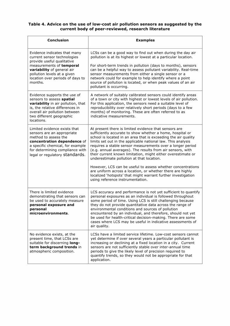
Table 4. Advice on the use of low-cost air pollution sensors as suggested by the current body of peer-reviewed, research literature

Conclusion

Examples

Evidence indicates that many current sensor technologies provide useful qualitative measurements of temporal variability of general air pollution levels at a given location over periods of days to months.

LCSs can be a good way to find out when during the day air pollution is at its highest or lowest at a particular location. For short-term trends in pollution (days to months), sensors can be a helpful way to assess pollutant variability. Real-time sensor measurements from either a single sensor or a network could for example to help identify where a point source of pollution is located, or when peak values of an air pollutant is occurring.

Evidence supports the use of sensors to assess spatial variability in air pollution, that is, the relative differences in overall air pollution between two different geographic locations.

A network of suitably calibrated sensors could identify areas of a town or city with highest or lowest levels of air pollution. For this application, the sensors need a suitable level of reproducibility over relatively short periods (days to a few months) of monitoring. These are often referred to as indicative measurements.

Limited evidence exists that sensors are an appropriate method to assess the concentration dependence of a specific chemical, for example for determining compliance with legal or regulatory standards.

At present there is limited evidence that sensors are sufficiently accurate to show whether a home, hospital or school is located in an area that is exceeding the air quality limits set out in the applicable national law. This analysis requires a stable sensor measurements over a longer period (e.g. annual averages). The results from air sensors, with their current known limitation, might either overestimate or underestimate pollution at that location. However, LCS can be useful to assess whether concentrations are uniform across a location, or whether there are highly localized ‘hotspots’ that might warrant further investigation using reference instrumentation.

There is limited evidence demonstrating that sensors can be used to accurately measure personal exposure and personal microenvironments.

LCS accuracy and performance is not yet sufficient to quantify personal exposures as an individual is followed throughout some period of time. Using LCS is still challenging because they do not provide quantitative data across the range of environmental conditions and sources of pollution encountered by an individual, and therefore, should not yet be used for health-critical decision-making. There are some cases where LCS may be useful in indicative assessments of air quality.

No evidence exists, at the present time, that LCSs are suitable for discerning long-term background trends in atmospheric composition.

LCSs have a limited service lifetime. Low-cost sensors cannot yet determine if over several years a particular pollutant is increasing or declining at a fixed location in a city. Current sensors are not sufficiently stable over inter-annual time periods to give the likely level of precision required to quantify trends, so they would not be appropriate for that application.

6. CONCLUSIONS The rapidly-growing scientific literature supports the use of low-cost air pollution sensors for certain applications but not others. LCSs are not currently a direct substitute for existing reference instruments or networks, but they are appropriate for other applications. It is important for prospective users to identify their specific application needs first, refer to the literature for studies that share similar characteristics, identify the likely limitations associated with using LCSs and then balance this against the value of the data that would be collected.

Previous studies in both the lab and field have shown that data quality from LCSs is variable among manufacturers and many different approaches to data quality are currently being taken. This can make the task to understanding likely data quality very challenging for users – even the same type of sensor can have different performance depending on the manufacturer. A general rule worth applying however is that LCSs should be treated like any other analytical instrument. They will likely require regular calibration and will show changes over the longer-term, for example drift, change in sensitivity and selectivity of response . The following factors should be assessed and considered in the context of LCS devices and their applicability:

(a) Range of temperature, humidity, and concentrations of the target pollutants; (b) Detection limits and possible ceiling values; (c) Stability under different environmental conditions to determine applicability for

outdoor, indoor, personal, or mobile sensing, including interference compounds; (d) For mobile sensing specifically, whether or not the readings of LCS devices are

affected by movement and can produce a useful measurement in the timescale required for the sampling application.

There is currently limited use of LCSs to support regulatory activities due to their current uncertainties and lack of certification of use, but this may change in the future. However, there is room in regulatory applications for using devices that do not meet the certified standards. For example, if the LCS were able to meet the data quality objectives documented in the framework of the Indicative Measurements of the EU Directive on Ambient Air (2008/50/EC), such an application would be possible. This regulatory standard is less stringent than the Fixed Measurements of the Directive that can be addressed by reference instruments only. Data science techniques are likely to play an increasingly important role in improving LCS measurement quality and diversifying sensor applications. A number of cases in the current literature documented improvements in LCS performance statistics when e.g. machine-learning techniques were applied in calibration protocols relative to other statistical methods, such as e.g. multiple linear regression, for multiple sensors. With LCS, the domains of public health, atmospheric chemistry, and regulatory decision-making can be empowered with data-driven insight.

Low-cost sensors are not currently a direct substitute for reference instruments or networks.

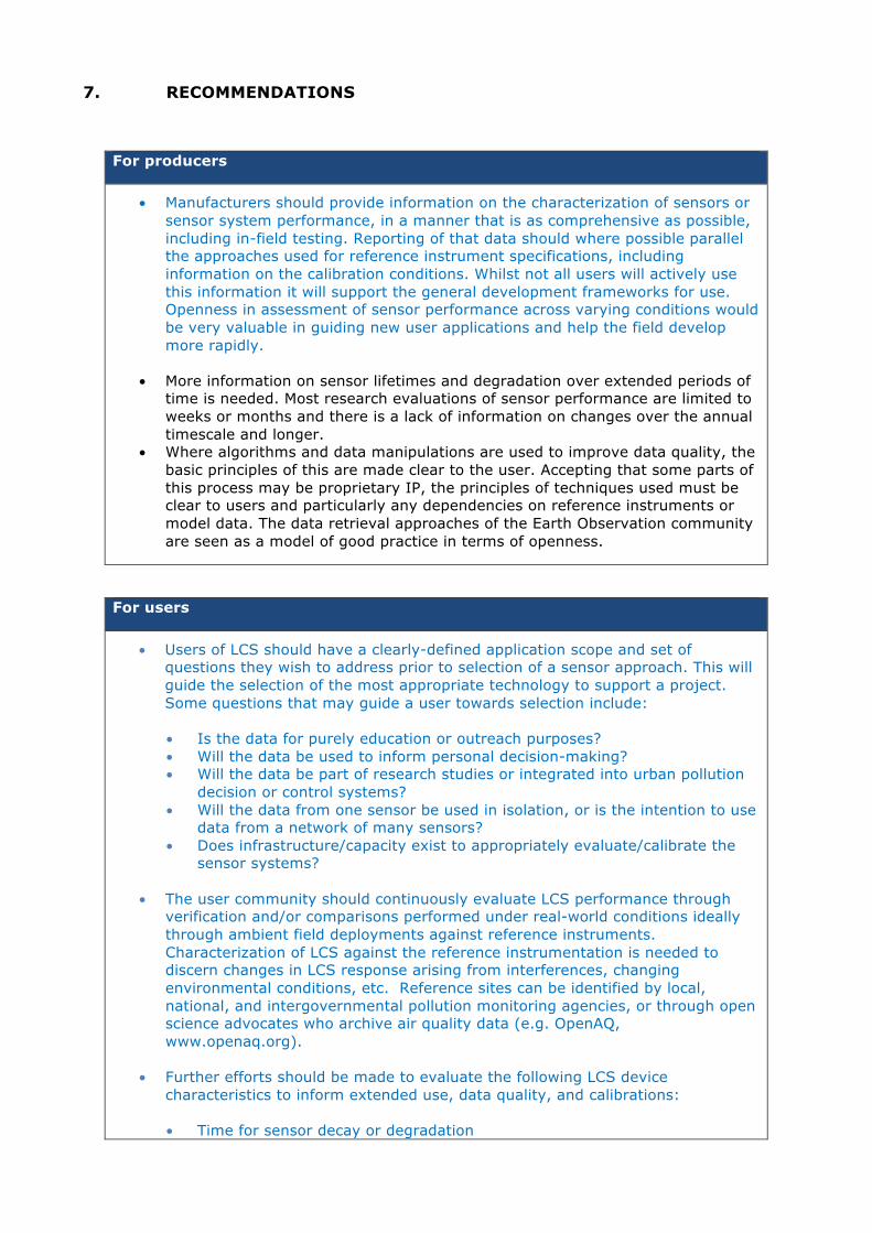
7. RECOMMENDATIONS

For producers

• Manufacturers should provide information on the characterization of sensors or sensor system performance, in a manner that is as comprehensive as possible, including in-field testing. Reporting of that data should where possible parallel the approaches used for reference instrument specifications, including information on the calibration conditions. Whilst not all users will actively use this information it will support the general development frameworks for use. Openness in assessment of sensor performance across varying conditions would be very valuable in guiding new user applications and help the field develop more rapidly.

• More information on sensor lifetimes and degradation over extended periods of time is needed. Most research evaluations of sensor performance are limited to weeks or months and there is a lack of information on changes over the annual timescale and longer.

• Where algorithms and data manipulations are used to improve data quality, the basic principles of this are made clear to the user. Accepting that some parts of this process may be proprietary IP, the principles of techniques used must be clear to users and particularly any dependencies on reference instruments or model data. The data retrieval approaches of the Earth Observation community are seen as a model of good practice in terms of openness.

For users

• Users of LCS should have a clearly-defined application scope and set of questions they wish to address prior to selection of a sensor approach. This will guide the selection of the most appropriate technology to support a project. Some questions that may guide a user towards selection include: • Is the data for purely education or outreach purposes? • Will the data be used to inform personal decision-making? • Will the data be part of research studies or integrated into urban pollution

decision or control systems? • Will the data from one sensor be used in isolation, or is the intention to use

data from a network of many sensors? • Does infrastructure/capacity exist to appropriately evaluate/calibrate the

sensor systems?

• The user community should continuously evaluate LCS performance through verification and/or comparisons performed under real-world conditions ideally through ambient field deployments against reference instruments. Characterization of LCS against the reference instrumentation is needed to discern changes in LCS response arising from interferences, changing environmental conditions, etc. Reference sites can be identified by local, national, and intergovernmental pollution monitoring agencies, or through open science advocates who archive air quality data (e.g. OpenAQ, www.openaq.org).

• Further efforts should be made to evaluate the following LCS device

characteristics to inform extended use, data quality, and calibrations:

• Time for sensor decay or degradation

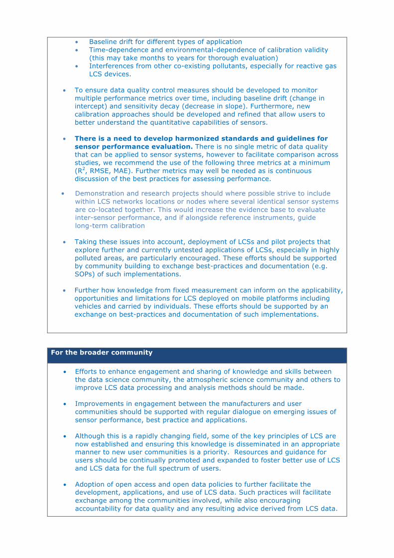
• Baseline drift for different types of application • Time-dependence and environmental-dependence of calibration validity

(this may take months to years for thorough evaluation) • Interferences from other co-existing pollutants, especially for reactive gas

LCS devices.

• To ensure data quality control measures should be developed to monitor multiple performance metrics over time, including baseline drift (change in intercept) and sensitivity decay (decrease in slope). Furthermore, new calibration approaches should be developed and refined that allow users to better understand the quantitative capabilities of sensors.

• There is a need to develop harmonized standards and guidelines for

sensor performance evaluation. There is no single metric of data quality that can be applied to sensor systems, however to facilitate comparison across studies, we recommend the use of the following three metrics at a minimum (R2, RMSE, MAE). Further metrics may well be needed as is continuous discussion of the best practices for assessing performance.

• Demonstration and research projects should where possible strive to include within LCS networks locations or nodes where several identical sensor systems are co-located together. This would increase the evidence base to evaluate inter-sensor performance, and if alongside reference instruments, guide long-term calibration

• Taking these issues into account, deployment of LCSs and pilot projects that

explore further and currently untested applications of LCSs, especially in highly polluted areas, are particularly encouraged. These efforts should be supported by community building to exchange best-practices and documentation (e.g. SOPs) of such implementations.

• Further how knowledge from fixed measurement can inform on the applicability,

opportunities and limitations for LCS deployed on mobile platforms including vehicles and carried by individuals. These efforts should be supported by an exchange on best-practices and documentation of such implementations.

For the broader community

• Efforts to enhance engagement and sharing of knowledge and skills between the data science community, the atmospheric science community and others to improve LCS data processing and analysis methods should be made.

• Improvements in engagement between the manufacturers and user

communities should be supported with regular dialogue on emerging issues of sensor performance, best practice and applications.

• Although this is a rapidly changing field, some of the key principles of LCS are

now established and ensuring this knowledge is disseminated in an appropriate manner to new user communities is a priority. Resources and guidance for users should be continually promoted and expanded to foster better use of LCS and LCS data for the full spectrum of users.

• Adoption of open access and open data policies to further facilitate the

development, applications, and use of LCS data. Such practices will facilitate exchange among the communities involved, while also encouraging accountability for data quality and any resulting advice derived from LCS data.

• Adopt and utilize best-practices for data management and documentation of associated data regarding implementation conditions. This can be based on existing and de novo approaches to data management and documentation.

• Continue to support existing activities for the validation and/or verification for

LCS and consider expanding to a wider range of environmental and pollution conditions. Such evaluation programmes or centres should be distributed worldwide to capture the variations in measurement environments, and underpin as a resource the geographically diverse user communities that may want to adopt LCS approaches in the future.

ANNEX 1 Low-cost air sensors have a range of known issues. Sensor systems can be designed

to overcome these issues such as cross-sensitivity, interference, correction, etc. This is an incomplete list, but is provided to offer a prospective LCS user with an

understanding of the types of limitations of many of these sensor types.

Sensor type Pollutant Known issue (effect) with sensors

Electrochemical Ozone (O3) Relative humidity Temperature Cross-sensitivity of oxidizing gases (e.g. NO2, H2S, Cl2) Long term stability (ageing or drift)

Nitrogen Dioxide (NO2) Relative humidity Temperature Cross-sensitivity of oxidizing gases (e.g. O3, H2S, Cl2) Long term stability (ageing or drift)

Sulfur Dioxide (SO2) Relative humidity Temperature Cross-sensitivity of reducing gases (e.g. NO2, H2S) Long term stability (ageing or drift)

Carbon monoxide (CO) Relative humidity Temperature Cross-sensitivity of reducing gases (e.g. H2S, SO2, CH4, Alcohols, NH3[MG1] , etc.) Long term stability (ageing or drift)

Metal oxide Ozone (O3) Response time > 5 min Sensor response is not linear Relative humidity Temperature Long term stability (drift) Varying baseline after re-start

Nitrogen Dioxide (NO2) Response time > 5 min Sensor response is generally not linear Relative humidity Temperature Short and long-term stability(drift) Varying baseline after re-start

Sulfur Dioxide (SO2) Relative humidity Temperature Cross-sensitivity of reducing gases (e.g. H2S)

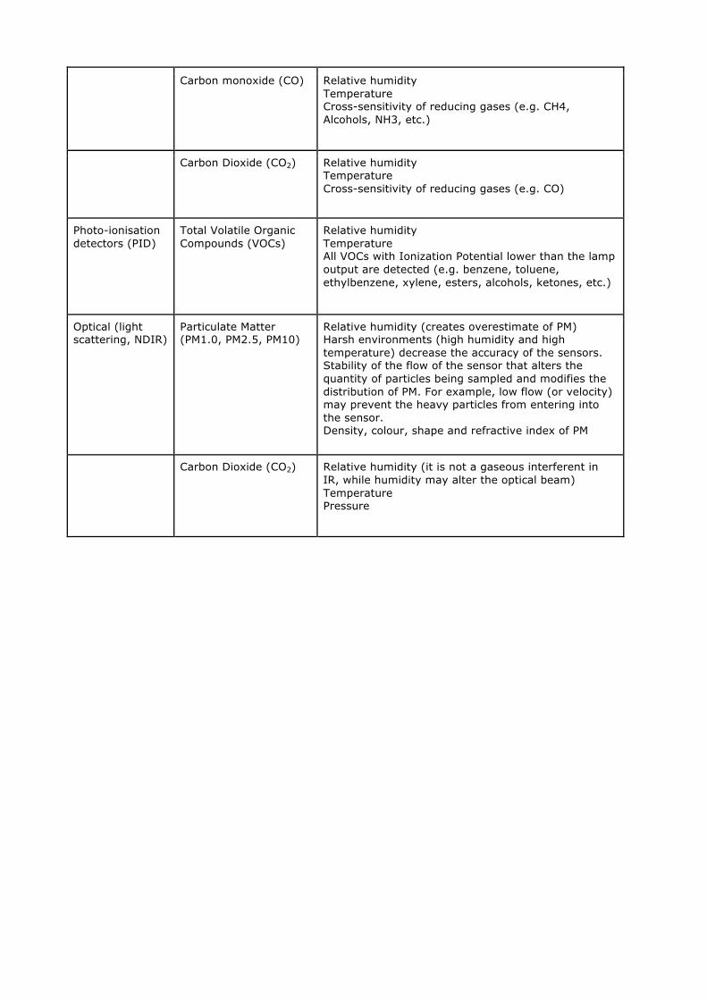
Carbon monoxide (CO) Relative humidity Temperature Cross-sensitivity of reducing gases (e.g. CH4, Alcohols, NH3, etc.)

Carbon Dioxide (CO2) Relative humidity Temperature Cross-sensitivity of reducing gases (e.g. CO)

Photo-ionisation detectors (PID)

Total Volatile Organic Compounds (VOCs)

Relative humidity Temperature All VOCs with Ionization Potential lower than the lamp output are detected (e.g. benzene, toluene, ethylbenzene, xylene, esters, alcohols, ketones, etc.)

Optical (light scattering, NDIR)

Particulate Matter (PM1.0, PM2.5, PM10)

Relative humidity (creates overestimate of PM) Harsh environments (high humidity and high temperature) decrease the accuracy of the sensors. Stability of the flow of the sensor that alters the quantity of particles being sampled and modifies the distribution of PM. For example, low flow (or velocity) may prevent the heavy particles from entering into the sensor. Density, colour, shape and refractive index of PM

Carbon Dioxide (CO2) Relative humidity (it is not a gaseous interferent in IR, while humidity may alter the optical beam) Temperature Pressure

REFERENCES

Aleixandre, M., Gerboles, M., 2012a. Review of Small Commercial Sensors for Indicative Monitoring of Ambient Gas. Chemical Engineering Transactions 30, 169-174.

Aleixandre, M., Gerboles, M., 2012b. Review of Small Commercial Sensors for Indicative Monitoring of Ambient Gas CHEMICAL ENGINEERING TRANSACTIONS 30.

Baron, R., Saffell, J., 2017. Amperometric Gas Sensors as a Low Cost Emerging Technology Platform for Air Quality Monitoring Applications: A Review. ACS Sensors 2, 1553-1566.

Borrego, C., Costa, A.M., Ginja, J., Amorim, M., Coutinho, M., Karatzas, K., Sioumis, T., Katsifarakis, N., Konstantinidis, K., De Vito, S., Esposito, E., Smith, P., André, N., Gérard, P., Francis, L.A., Castell, N., Schneider, P., Viana, M., Minguillón, M.C., Reimringer, W., Otjes, R.P., von Sicard, O., Pohle, R., Elen, B., Suriano, D., Pfister, V., Prato, M., Dipinto, S., Penza, M., 2016. Assessment of air quality microsensors versus reference methods: The EuNetAir joint exercise. Atmospheric Environment 147, 246-263.

Caron, A., Redon, N., Thevenet, F., Hanoune, B., Coddeville, P., 2016. Performances and limitations of electronic gas sensors to investigate an indoor air quality event. Building and Environment 107, 19-28.

Castell, N., Dauge, F.R., Schneider, P., Vogt, M., Lerner, U., Fishbain, B., Broday, D., Bartonova, A., 2017. Can commercial low-cost sensor platforms contribute to air quality monitoring and exposure estimates? Environment International 99, 293-302.

Chen, L.J., Ho, Y.H., Hsieh, H.H., Huang, S.T., Lee, H.C., Mahajan, S., 2017. ADF: an Anomaly Detection Framework for Large-scale PM2.5 Sensing Systems. IEEE Internet of Things Journal PP, 1-1.

Chen, L.J., Ho, Y.H., Hsieh, H.H., Huang, S.T., Lee, H.C., Mahajan, S., 2018. ADF: an Anomaly Detection Framework for Large-scale PM2.5 Sensing Systems. IEEE Internet of Things Journal.

Collier-Oxandale, A., Hannigan, M.P., Casey, J.G., Piedrahita, R., Ortega, J., Halliday, H., Johnston, J., 2018. Assessing a low-cost methane sensor quantification system for use in complex rural and urban environments. Atmos. Meas. Tech. Discuss. 2018, 1-35.

Cross, E.S., Williams, L.R., Lewis, D.K., Magoon, G.R., Onasch, T.B., Kaminsky, M.L., Worsnop, D.R., Jayne, J.T., 2017a. Use of electrochemical sensors for measurement of air pollution: correcting interference response and validating measurements. Atmos. Meas. Tech. 10, 3575-3588.

Cross, E.S., Williams, L.R., Lewis, D.K., Magoon, G.R., Onasch, T.B., Kaminsky, M.L., Worsnop, D.R., Jayne, J.T., 2017b. The use of electrochemical sensors for measurement of air pollution: correcting interference response and validating measurements. Atmos. Meas. Tech. 10, 3575-3588.

De Vito, S., Piga, M., Martinotto, L., Di Francia, G., 2009. Co, NO 2 and NO x urban pollution monitoring with on-field calibrated electronic nose by automatic bayesian regularization. Sensors and Actuators B: Chemical 143, 182-191.

Eugster, W., Kling, G.W., 2012a. Performance of a low-cost methane sensor for ambient concentration measurements in preliminary studies. Atmos. Meas. Tech. 5, 1925-1934.

Eugster, W., Kling, G.W., 2012b. Performance of a low-cost methane sensor for ambient concentration measurements in preliminary studies. Atmos. Meas. Tech. 5, 1925-1934.

Fine, G.F., Cavanagh, L.M., Afonja, A., Binions, R., 2010. Metal Oxide Semi-Conductor Gas Sensors in Environmental Monitoring. Sensors 10, 5469.

Hagan, D.H., Isaacman-VanWertz, G., Franklin, J.P., Wallace, L.M.M., Kocar, B.D., Heald, C.L., Kroll, J.H., 2018. Calibration and assessment of electrochemical air quality sensors by co-location with regulatory-grade instruments. Atmos. Meas. Tech. 11, 315-328.

Holstius, D.M., Pillarisetti, A., Smith, K.R., Seto, E., 2014. Field calibrations of a low-cost aerosol sensor at a regulatory monitoring site in California. Atmos. Meas. Tech. 7, 1121-1131.

Jerrett, M., Donaire-Gonzalez, D., Popoola, O., Jones, R., Cohen, R.C., Almanza, E., de Nazelle, A., Mead, I., Carrasco-Turigas, G., Cole-Hunter, T., Triguero-Mas, M., Seto, E., Nieuwenhuijsen, M., 2017. Validating novel air pollution sensors to improve exposure estimates for epidemiological analyses and citizen science. Environmental Research 158, 286-294.

Jiao, W., Hagler, G., Williams, R., Sharpe, R., Brown, R., Garver, D., Judge, R., Caudill, M., Rickard, J., Davis, M., Weinstock, L., Zimmer-Dauphinee, S., Buckley, K., 2016. Community Air Sensor Network (CAIRSENSE) project: evaluation of low-cost sensor performance in a suburban environment in the southeastern United States. Atmos. Meas. Tech. 9, 5281-5292.

Jovašević-Stojanović, M., Bartonova, A., Topalović, D., Lazović, I., Pokrić, B., Ristovski, Z., 2015. On the use of small and cheaper sensors and devices for indicative citizen-based monitoring of respirable particulate matter. Environmental Pollution, 206, 696-704.

Kim, J., Shusterman, A.A., Lieschke, K.J., Newman, C., Cohen, R.C., 2017. The BErkeley Atmospheric CO2 Observation Network: Field Calibration and Evaluation of Low-cost Air Quality Sensors. Atmos. Meas. Tech. Discuss. 2017.

Kotsev, A., Schade, S., Craglia, M., Gerboles, M., Spinelle, L., Signorini, M., 2016. Next Generation Air Quality Platform: Openness and Interoperability for the Internet of Things. Sensors 16, 403.

Kumar, P., Morawska, L., Martani, C., Biskos, G., Neophytou, M., Di Sabatino, S., Bell, M., Norford, L., Britter, R., 2015. The rise of low-cost sensing for managing air pollution in cities. Environment International 75, 199-205.

Kunz, M., Lavric, J.V., Gerbig, C., Tans, P., Neff, D., Hummelgård, C., Martin, H., Rödjegård, H., Wrenger, B., Heimann, M., 2017. COCAP: A carbon dioxide analyser for small unmanned aircraft systems. Atmos. Meas. Tech. Discuss. 2017, 1-29.

Lewis, A., D Lee, J., Edwards, P., Shaw, M., Evans, M., Moller, S., R Smith, K., Ellis, M., Gillott, S., White, A., W Buckley, J., 2016. Evaluating the performance of low cost chemical sensors for air pollution research.

Lewis, A., Edwards, P., 2016. Validate personal air-pollution sensors.

Lewis, A.C., Zellweger, C., Schultz, M.G., Tarasova, O.A., (GAW), R.G.S.A.G., 2017. Technical advice note on lower cost air pollution sensors. World Meteorological Organization and Global Atmosphere Watch.

Lin, C., Gillespie, J., Schuder, M.D., Duberstein, W., Beverland, I.J., Heal, M.R., 2015. Evaluation and calibration of Aeroqual series 500 portable gas sensors for accurate measurement of ambient ozone and nitrogen dioxide. Atmospheric Environment 100, 111-116.

Masson, N., Piedrahita, R., Hannigan, M., 2015. Approach for quantification of metal oxide type semiconductor gas sensors used for ambient air quality monitoring. Sensors and Actuators B: Chemical 208, 339-345.

Mead, M.I., Popoola, O.A.M., Stewart, G.B., Landshoff, P., Calleja, M., Hayes, M., Baldovi, J.J., McLeod, M.W., Hodgson, T.F., Dicks, J., Lewis, A., Cohen, J., Baron, R., Saffell, J.R., Jones, R.L., 2013. The use of electrochemical sensors for monitoring urban air quality in low-cost, high-density networks. Atmospheric Environment 70, 186-203.

Moltchanov, S., Levy, I., Etzion, Y., Lerner, U., Broday, D., Fishbain, B., 2014. On the feasibility of measuring urban air pollution by wireless distributed sensor networks.

Mueller, M., Meyer, J., Hueglin, C., 2017. Design of an ozone and nitrogen dioxide sensor unit and its long-term operation within a sensor network in the city of Zurich. Atmos. Meas. Tech. 10, 3783-3799.

Penza, M., Suriano, D., Pfister, V., Prato, M., Cassano, G., 2017. Urban Air Quality Monitoring with Networked Low-Cost Sensor-Systems. Proceedings 1, 573.

Penza, M., Suriano, D., Villani, M.G., Spinelle, L., Gerboles, M., 2014. Towards air quality indices in smart cities by calibrated low-cost sensors applied to networks, IEEE SENSORS 2014 Proceedings, pp. 2012-2017.

Peterson, P., Aujla, A., Grant, K., Brundle, A., Thompson, M., Vande Hey, J., Leigh, R., 2017. Practical Use of Metal Oxide Semiconductor Gas Sensors for Measuring Nitrogen Dioxide and Ozone in Urban Environments. Sensors 17, 1653.

Piedrahita, R., Xiang, Y., Masson, N., Ortega, J., Collier, A., Jiang, Y., Li, K., Dick, R.P., Lv, Q., Hannigan, M., Shang, L., 2014. The next generation of low-cost personal air quality sensors for quantitative exposure monitoring. Atmos. Meas. Tech. 7, 3325-3336.

Popoola, O.A.M., Stewart, G.B., Mead, M.I., Jones, R.L., 2016. Development of a baseline-temperature correction methodology for electrochemical sensors and its implications for long-term stability. Atmospheric Environment 147, 330-343.

Rai, A.C., Kumar, P., Pilla, F., Skouloudis, A.N., Di Sabatino, S., Ratti, C., Yasar, A., Rickerby, D., 2017. End-user perspective of low-cost sensors for outdoor air pollution monitoring. Science of The Total Environment 607-608, 691-705.

Rigby, M., Prinn, R.G., Fraser, P.J., Simmonds, P.G., Langenfelds, R.L., Huang, J., Cunnold, D.M., Steele, L.P., Krummel, P.B., Weiss, R.F., O'Doherty, S., Salameh, P.K., Wang, H.J., Harth, C.M., Mühle, J., Porter, L.W., 2008. Renewed growth of atmospheric methane. Geophysical Research Letters 35, n/a-n/a.

Sadighi, K., Coffey, E., Polidori, A., Feenstra, B., Lv, Q., Henze, D.K., Hannigan, M., 2017. Intra-urban spatial variability of surface ozone and carbon dioxide in Riverside, CA: viability and validation of low-cost sensors. Atmos. Meas. Tech. Discuss. 2017, 1-30.

Shusterman, A.A., Teige, V.E., Turner, A.J., Newman, C., Kim, J., Cohen, R.C., 2016. The BErkeley Atmospheric CO2 Observation Network: initial evaluation. Atmos. Chem. Phys. 16, 13449-13463.

Smith, K.R., Edwards, P.M., Evans, M.J., Lee, J.D., Shaw, M.D., Squires, F., Wilde, S., Lewis, A.C., 2017. Clustering approaches to improve the performance of low cost air pollution sensors. Faraday Discussions 200, 621-637.

Snyder, E.G., Watkins, T.H., Solomon, P.A., Thoma, E.D., Williams, R.W., Hagler, G.S.W., Shelow, D., Hindin, D.A., Kilaru, V.J., Preuss, P.W., 2013. The Changing Paradigm of Air Pollution Monitoring. Environmental Science & Technology 47, 11369-11377.

Spinelle, L., Gerboles, M., Aleixandre, M., 2013. Protocol of evaluation and calibration of low-cost gas sensors for the monitoring of air pollution, Publications Office of the European Union.

Spinelle, L., Gerboles, M., Aleixandre, M., 2015a. Performance Evaluation of Amperometric Sensors for the Monitoring of O3 and NO2 in Ambient Air at ppb Level. Procedia Engineering 120, 480-483.

Spinelle, L., Gerboles, M., Aleixandre, M., Bonavitacola, F., 2016. Evaluation of Metal Oxides Sensors for the Monitoring of O3 in Ambient Air at Ppb Level. Italian Association of Chemical Engineering - AIDIC.

Spinelle, L., Gerboles, M., Kok, G., Persijn, S., Sauerwald, T., 2017a. Review of Portable and Low-Cost Sensors for the Ambient Air Monitoring of Benzene and Other Volatile Organic Compounds. Sensors (Basel, Switzerland) 17.

Spinelle, L., Gerboles, M., Villani, M.G., Aleixandre, M., Bonavitacola, F., 2015b. Field calibration of a cluster of low-cost available sensors for air quality monitoring. Part A: Ozone and nitrogen dioxide. Sensors and Actuators B: Chemical 215, 249-257.

Spinelle, L., Gerboles, M., Villani, M.G., Aleixandre, M., Bonavitacola, F., 2017b. Field calibration of a cluster of low-cost commercially available sensors for air quality monitoring. Part B: NO, CO and CO2. Sensors and Actuators B: Chemical 238, 706-715.

Sun, L., Wong, K., Wei, P., Ye, S., Huang, H., Yang, F., Westerdahl, D., Louie, P., Luk, C., Ning, Z., 2016. Development and Application of a Next Generation Air Sensor Network for the Hong Kong Marathon 2015 Air Quality Monitoring. Sensors 16, 211.

Suto, H., Inoue, G., 2010. A New Portable Instrument for In Situ Measurement of Atmospheric Methane Mole Fraction by Applying an Improved Tin Dioxide–Based Gas Sensor, Journal of Atmospheric and Oceanic Technology 27, 1175-1184.

Turner, A.J., Shusterman, A.A., McDonald, B.C., Teige, V., Harley, R.A., Cohen, R.C., 2016. Network design for quantifying urban CO2 emissions: assessing trade-offs between precision and network density. Atmos. Chem. Phys. 16, 13465-13475.

Wang, C., Yin, L., Zhang, L., Xiang, D., Gao, R., 2010. Metal Oxide Gas Sensors: Sensitivity and Influencing Factors. Sensors 10, 2088.

Wetchakun, K., Samerjai, T., Tamaekong, N., Liewhiran, C., Siriwong, C., Kruefu, V., Wisitsoraat, A., Tuantranont, A., Phanichphant, S., 2011. Semiconducting metal oxides as sensors for environmentally hazardous gases. Sensors and Actuators B: Chemical 160, 580-591.

Williams, D., S Henshaw, G., Bart, M., Laing, G., Wagner, J., Naisbitt, S., Salmond, J., 2013. Validation of low-cost ozone measurement instruments suitable for use in an air-quality monitoring network.

Williams, D.E., Salmond, J., Yung, Y.F., Akaji, J., Wright, B., Wilson, J., Henshaw, G.S., Wells, D.B., Ding, G., Wagner, J., Laing, G., 2009. Development of low-cost ozone and nitrogen dioxide measurement instruments suitable for use in an air quality monitoring network, 2009 IEEE Sensors, pp. 1099-1104.

Williams, R., Long, R., Beaver, M., Kaufman, A., Zeiger, F., Heimbinder, M., Hang, I., Yap, R., Acharya, B., Ginwald, B., Kupcho, K., Robinson, S., Zaouak, O., Aubert, B., Hannigan, M., Piedrahita, R., Masson, N., Moran, B., Rook, M., Heppner, P., Cogar, C., Nikzad, N., Griswold, W., 2014. Sensor Evaluation Report. U.S. Environmental Protection Agency.

Zimmerman, N., Presto, A.A., Kumar, S.P.N., Gu, J., Hauryliuk, A., Robinson, E.S., Robinson, A.L., Subramanian, R., 2018. A machine learning calibration model using random forests to improve sensor performance for lower-cost air quality monitoring. Atmos. Meas. Tech. 11, 291-313.