low-complexity polynomial channel estimation in large
TRANSCRIPT

arX
iv:1
401.
5703
v2 [
cs.IT
] 5
Dec
201
41
Low-Complexity Polynomial Channel Estimation inLarge-Scale MIMO with Arbitrary Statistics
Nafiseh Shariati,Student Member, IEEE,Emil Bjornson,Member, IEEE,Mats Bengtsson,Senior Member, IEEE,and Merouane Debbah,Senior Member, IEEE
Abstract—This paper considers pilot-based channel estimationin large-scale multiple-input multiple-output (MIMO) com muni-cation systems, also known as “massive MIMO”, where there arehundreds of antennas at one side of the link. Motivated by thefact that computational complexity is one of the main challengesin such systems, a set of low-complexity Bayesian channel estima-tors, coinedPolynomial ExpAnsion CHannel (PEACH) estimators,are introduced for arbitrary channel and interference statistics.While the conventional minimum mean square error (MMSE)estimator has cubic complexity in the dimension of the covariancematrices, due to an inversion operation, our proposed estimatorssignificantly reduce this to square complexity by approximatingthe inverse by aL-degree matrix polynomial. The coefficients ofthe polynomial are optimized to minimize the mean square error(MSE) of the estimate.
We show numerically that near-optimal MSEs are achievedwith low polynomial degrees. We also derive the exact com-putational complexity of the proposed estimators, in termsofthe floating-point operations (FLOPs), by which we prove thatthe proposed estimators outperform the conventional estimatorsin large-scale MIMO systems of practical dimensions whileproviding a reasonable MSEs. Moreover, we show thatL needsnot scale with the system dimensions to maintain a certainnormalized MSE. By analyzing different interference scenarios,we observe that the relative MSE loss of using the low-complexityPEACH estimators is smaller in realistic scenarios with pilot con-tamination. On the other hand, PEACH estimators are not wellsuited for noise-limited scenarios with high pilot power; therefore,we also introduce the low-complexity diagonalized estimatorthat performs well in this regime. Finally, we also investigatenumerically how the estimation performance is affected by havingimperfect statistical knowledge. High robustness is achieved forlarge-dimensional matrices by using a new covariance estimatewhich is an affine function of the sample covariance matrix anda regularization term.
Index Terms—Channel estimation, large-scale MIMO, polyno-mial expansion, pilot contamination, spatial correlation.
Copyright (c) 2013 IEEE. Personal use of this material is permitted.However, permission to use this material for any other purposes must beobtained from the IEEE by sending a request to [email protected].
N. Shariati and M. Bengtsson are with the Department of Signal Processing,ACCESS Linnaeus Centre, KTH Royal Institute of Technology,Stockholm,Sweden (e-mail:{nafiseh, mats.bengtsson}@ee.kth.se).
E. Bjornson was with the Alcatel-Lucent Chair on Flexible Radio, Supelec,Gif-sur-Yvette, France, and with the Department of Signal Processing, KTHRoyal Institute of Technology, Stockholm, Sweden. He is currently with theDepartment of Electrical Engineering (ISY), Linkoping University, Linkoping,Sweden (email: [email protected]).
M. Debbah is with the Alcatel-Lucent Chair on Flexible Radio, SUPELEC,Gif-sur-Yvette, France (e-mail:[email protected]).
This work was presented in part at IEEE Symposium on Personal, Indoor,Mobile and Radio Communications (PIMRC), London, UK, Sept.2013. [1]
E. Bjornson is funded by the International Postdoc Grant 2012-228 fromThe Swedish Research Council. This research has been supported by the ERCStarting Grant 305123 MORE (Advanced Mathematical Tools for ComplexNetwork Engineering).
I. I NTRODUCTION
MIMO techniques can bring huge improvements in spectralefficiency to wireless systems, by increasing the spatial reusethrough spatial multiplexing [2]. While8×8 MIMO transmis-sions have found its way into recent communication standards,such as LTE-Advanced [3], there is an increasing interest fromacademy and industry to equip base stations (BSs) with muchlarger arrays with several hundreds of antenna elements [4]–[9]. Such large-scale MIMO, or “massive MIMO”, techniquescan give unprecedented spatial resolution and array gain, thusenabling a very dense spatial reuse that potentially can keep upwith the rapidly increasing demand for wireless connectivityand need for high energy efficiency.
The antenna elements in large-scale MIMO can be eithercollocated in one- or multi-dimensional arrays or distributedover a larger area (e.g., on the facade or the windows ofbuildings) [8]. Apart from increasing the spectral efficiencyof conventional wireless systems, which operate at carrierfrequencies of one or a few GHz, the use of massive antennaconfigurations is also a key enabler for high-rate transmissionsin mm-Wave bands, where there are plenty of unused spectrumtoday [9]. In particular, the array gain of large-scale MIMOmitigates the large propagation losses at such high frequen-cies and 256 antenna elements with half-wavelength minimalspacing can be packed into6× 6 cm at 80 GHz [9].
The majority of previous works on large-scale MIMO (see[4]–[8] and references therein) considers scenarios whereBSs equipped with many antennas communicate with single-antenna user terminals (UTs). While this assumption allowsfor closed-form characterizations of the asymptotic throughput(when the number of antennas and UTs grow large), we canexpect practical UTs to be equipped with multiple antennasas well—this is indeed the case already in LTE-Advanced [3].However, the limited form factor of terminals typically allowsfor fewer antennas than at the BSs, but the number might stillbe unconventionally large in mm-Wave communications.
A major limiting factor in large-scale MIMO is the availabil-ity of accurate instantaneous channel state information (CSI).This is since high spatial resolution can only be exploitedif the propagation environment is precisely known. CSI istypically acquired by transmitting predefined pilot signals andestimating the channel coefficients from the received signals[10]–[15]. The pilot overhead is proportional to the numberoftransmit antennas, thus it is commonly assumed that the pilotsare sent from the array with the smallest number of antennasand used for transmission in both directions by exploiting

2
channel reciprocity in time-division duplex (TDD) mode.The instantaneous channel matrix is acquired from the
received pilot signal by applying an appropriate estimationscheme. The Bayesian MMSE estimator is optimal if thechannel statistics are known [12]–[16], while the minimum-variance unbiased (MVU) estimator is applied otherwise [12].These channel estimators basically solve a linear system ofequations, or equivalently multiply the received pilot signalwith an inverse of the covariance matrices. This is a math-ematical operation with cubic computational complexity inthe matrix dimension, which is the product of the number ofantennas at the receiver (at the order of 100) and the length ofthe pilot sequence (at the order of 10). Evidently, this operationis extremely computationally expensive in large-scale MIMOsystems, thus the MMSE and MVU channel estimates cannotbe computed within a reasonable period of time. The highcomputational complexity can be avoided under propagationconditions where all covariance matrices are diagonal, butlarge-scale MIMO channels typically have a distinct spatialchannel correlation due to insufficient antenna spacing andrichness of the propagation environment [7]. The spatialcorrelation decreases the estimation errors [15], but onlyif anappropriate estimator is applied. Moreover, the necessarypilotreuse in cellular networks creates spatially correlated inter-cellinterference, known aspilot contamination, which reduces theestimation performance and spectral efficiency [5]–[7], [10],[11].
Polynomial expansion (PE)is a well-known technique toreduce the complexity of large-dimensional matrix inversions[17]. Similar to classic Taylor series expansions for scalarfunctions, PE approximates a matrix function by anL-degreematrix polynomial. PE has a long history in the field of signalprocessing for multiuser detection/equalization, where both thedecorrelating detector and the linear MMSE detector involvematrix inversions [17]–[22]. PE-based detectors are versatilesince the structure enables simple multistage/pipelined hard-ware implementation [17] using only additions and multiplica-tions. The degreeL basically describes the accuracy to whichthe inversion of each eigenvalue is approximated, thus thedegree needs not scale with the system dimensions to achievenear optimal performance [20]. Instead,L is simply selectedto balance between computational complexity and detectionperformance. A main problem is to select the coefficientsof the polynomial to achieve high performance at smallL;the optimal coefficients are expensive to compute [17], butalternatives based on appropriate scalings [18], [21], [23] andasymptotic analysis [19], [22] exist. Recently, PE has alsobeenused to reduce the precoding complexity in large-scale MIMOsystems [24]–[26], and high performance was achieved byoptimizing the matrix polynomials using asymptotic analysis.
The optimization of the polynomial coefficients is the keyto high performance when using PE. Since the system mod-els and performance metrics are fundamentally different inmultiuser detection and precoding, the derivation of optimaland low-complexity suboptimal coefficients become two verydifferent problems in these two applications. In this paper, weconsider a new signal processing application for PE, namelypilot-based estimation of MIMO channels. We apply the PE
technique to approximate the MMSE estimator and therebyobtain a new set of low-complexity channel estimators that wecoin Polynomial ExpAnsion CHannel (PEACH)estimators.1 Amain contribution of the paper is to optimize the coefficientsof the polynomial to yield low MSE at any fixed polynomialdegreeL, while keeping the low complexity. The PEACH es-timators are evaluated under different propagation/interferenceconditions and show remarkably good performance at lowpolynomial degrees. An important property is thatL needsnot scale with the number of antennas to maintain a fixednormalized MSE loss (as compared to MMSE estimation).However,L should increase with the transmit power to keepa fixed loss, while it can actually be decreased as the interfer-ence becomes stronger. The computational complexity of thePEACH estimators and conventional MMSE/MVU estimatorsare compared analytically. This reveals that the proposedestimators have smaller complexity exponents. The numeri-cal results confirm that much fewer FLOPs are required tocompute the PEACH estimators in large-scale MIMO systemsof practical dimensions. Finally, thediagonalized estimatoris introduced with even lower complexity and it is shown inwhich scenarios it is suitable.
A. Outline
The organization of this paper is as follows. In SectionII, we describe the system model and formulate the problemof estimating channel coefficients for a large-scale MIMOcommunication system where the computational complexity isa major issue. Following the Bayesian philosophy, we proposea set of low-complexity estimators in Section III and providean exact complexity analysis. In Section IV, we numericallyevaluate the performance of the proposed estimators in dif-ferent interference scenarios where comparison is performedwith respect to conventional estimators. Finally, conclusionsare drawn in Section V.
B. Notation
Boldface (lower case) is used for column vectors,x, and(upper case) for matrices,X. Let XT , XH , andX−1 denotethe transpose, the conjugate transpose, and the inverse ofX,respectively. The Kronecker product ofX andY is denotedX⊗Y, vec(X) is the vector obtained by stacking the columnsof X, tr(X) denotes the trace,‖X‖F is the Frobenius norm,and ‖X‖2 is the spectral norm. The notation, denotesdefinitions, while the big-O notationO(Mx) describes thatthe complexity is bounded byCMx for some0 < C < ∞.A circularly symmetric complex Gaussian random vectorx isdenotedx ∼ CN (x,Q), wherex is the mean andQ is thecovariance matrix.
1After the submission of this paper, we became aware of the concurrentwork of [27] which also applies PE to reduce the complexity ofMMSEestimation. However, orthogonal frequency division multiplexing (OFDM)systems with a large number of subcarriers are considered in[27], whilelarge-scale single-carrier MIMO systems are our focus. This makes the systemmodels, analysis, and results non-overlapping.
3
Pilot signal
Transmitter
(Few antennas)
Receiver
(Very many antennas)
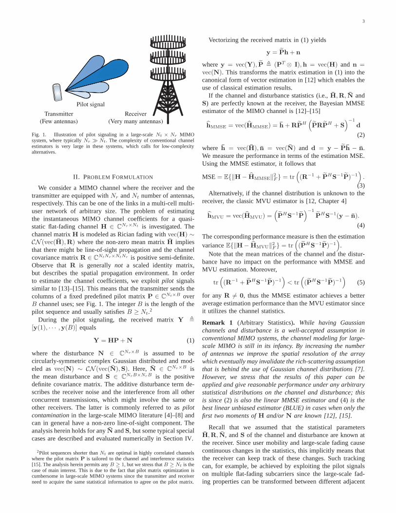
Fig. 1. Illustration of pilot signaling in a large-scaleNt × Nr MIMOsystem, where typicallyNr ≫ Nt. The complexity of conventional channelestimators is very large in these systems, which calls for low-complexityalternatives.
II. PROBLEM FORMULATION
We consider a MIMO channel where the receiver and thetransmitter are equipped withNr andNt number of antennas,respectively. This can be one of the links in a multi-cell multi-user network of arbitrary size. The problem of estimatingthe instantaneous MIMO channel coefficients for a quasi-static flat-fading channelH ∈ CNr×Nt is investigated. Thechannel matrixH is modeled as Rician fading withvec(H) ∼CN (vec(H),R) where the non-zero mean matrixH impliesthat there might be line-of-sight propagation and the channelcovariance matrixR ∈ CNtNr×NtNr is positive semi-definite.Observe thatR is generallynot a scaled identity matrix,but describes the spatial propagation environment. In orderto estimate the channel coefficients, we exploitpilot signalssimilar to [13]–[15]. This means that the transmitter sendsthecolumns of a fixed predefined pilot matrixP ∈ CNt×B overB channel uses; see Fig. 1. The integerB is the length of thepilot sequence and usually satisfiesB ≥ Nt.2
During the pilot signaling, the received matrixY ,[y(1), · · · ,y(B)] equals
Y = HP+N (1)
where the disturbanceN ∈ CNr×B is assumed to becircularly-symmetric complex Gaussian distributed and mod-eled asvec(N) ∼ CN (vec(N),S). Here, N ∈ CNr×B isthe mean disturbance andS ∈ CNrB×NrB is the positivedefinite covariance matrix. The additive disturbance term de-scribes the receiver noise and the interference from all otherconcurrent transmissions, which might involve the same orother receivers. The latter is commonly referred to aspilotcontaminationin the large-scale MIMO literature [4]–[8] andcan in general have a non-zero line-of-sight component. Theanalysis herein holds for anyN andS, but some typical specialcases are described and evaluated numerically in Section IV.
2Pilot sequences shorter thanNt are optimal in highly correlated channelswhere the pilot matrixP is tailored to the channel and interference statistics[15]. The analysis herein permits anyB ≥ 1, but we stress thatB ≥ Nt is thecase of main interest. This is due to the fact that pilot matrix optimization iscumbersome in large-scale MIMO systems since the transmitter and receiverneed to acquire the same statistical information to agree onthe pilot matrix.
Vectorizing the received matrix in (1) yields
y = Ph+ n
wherey = vec(Y), P , (PT ⊗ I),h = vec(H) and n =vec(N). This transforms the matrix estimation in (1) into thecanonical form of vector estimation in [12] which enables theuse of classical estimation results.
If the channel and disturbance statistics (i.e.,H,R, N andS) are perfectly known at the receiver, the Bayesian MMSEestimator of the MIMO channel is [12]–[15]
hMMSE = vec(HMMSE) = h+RPH(PRPH + S
)−1
d
(2)
where h = vec(H), n = vec(N) and d = y − Ph − n.We measure the performance in terms of the estimation MSE.Using the MMSE estimator, it follows that
MSE= E{‖H− HMMSE‖2F } = tr((R−1 + PHS−1P)−1
).
(3)Alternatively, if the channel distribution is unknown to the
receiver, the classic MVU estimator is [12, Chapter 4]
hMVU = vec(HMVU) =(PHS−1P
)−1
PHS−1(y − n).
(4)
The corresponding performance measure is then the estimationvarianceE{‖H− HMVU‖2F } = tr
((PHS−1P)−1
).
Note that the mean matrices of the channel and the distur-bance have no impact on the performance with MMSE andMVU estimation. Moreover,
tr((R−1 + PHS−1P)−1
)< tr
((PHS−1P)−1
)(5)
for any R 6= 0, thus the MMSE estimator achieves a betteraverage estimation performance than the MVU estimator sinceit utilizes the channel statistics.
Remark 1 (Arbitrary Statistics). While having Gaussianchannels and disturbance is a well-accepted assumption inconventional MIMO systems, the channel modeling for large-scale MIMO is still in its infancy. By increasing the numberof antennas we improve the spatial resolution of the arraywhich eventually may invalidate the rich-scattering assumptionthat is behind the use of Gaussian channel distributions [7].However, we stress that the results of this paper can beapplied and give reasonable performance under any arbitrarystatistical distributions on the channel and disturbance;thisis since(2) is also the linear MMSE estimator and(4) is thebest linear unbiased estimator (BLUE) in cases when only thefirst two moments ofH and/orN are known [12], [15].
Recall that we assumed that the statistical parametersH,R, N, andS of the channel and disturbance are known atthe receiver. Since user mobility and large-scale fading causecontinuous changes in the statistics, this implicitly means thatthe receiver can keep track of these changes. Such trackingcan, for example, be achieved by exploiting the pilot signalson multiple flat-fading subcarriers since the large-scale fad-ing properties can be transformed between different adjacent

4
subcarriers [28], [29]. Interestingly, the coherence timeofthe long-term statistics is relatively short; the measurementsin [30] observe coherence times of5–23 seconds, depend-ing on the propagation environment. High user velocity orrapid scheduling decisions in neighboring systems can furtherreduce the coherence time. More importantly, the numberof channel realizations within each coherence time of thestatistics is around13–126, according to [30]. This meansthat the matrix inversion in the MMSE estimator has to berecomputed frequently.
A. Complexity Issues in Large-Scale MIMO Systems
The main computational complexity when computing theMMSE and MVU estimators in (2) and (4) lies in solvinga linear system of equations or, equivalently, in computingthe matrix inversions directly. Both approaches have compu-tational complexities that scale asO(M3), whereM , BNr
is the matrix dimension.3 This complexity is relatively modestin conventional MIMO communication systems where2× 2,4× 4, or 8× 8 are typical configurations.
Recently, there is an increasing interest in large-scale MIMOsystems where there might be hundreds of antennas at oneside of the link [4]–[9]. To excite all channel dimensions, thepilot lengthB should be of the same order asNt. Large-scaleMIMO systems are therefore envisioned to operate in TDDmode and exploit channel reciprocity to always haveNt < Nr
in the channel estimation phase—Nr can even be orders ofmagnitude larger thanNt without degrading the estimationperformanceper antenna element.
Observe that in a potential future large-scale MIMO systemwith Nr = 200 and Nt = B = 20, the MMSE and MVUestimators would require inverting matrices of size4000×4000(or similarly, solving a linear system of equations with4000unknown variables) which has a complexity at the orderof 3.4 · 1011 floating-point operations, see Section III-E fordetails. This massive matrix manipulation needs to be redoneevery few seconds sinceR and S change due to mobility.Motivated by these facts, the purpose of this paper is todevelop alternative channel estimators that allow for balancingbetween computational/hardware complexity and estimationperformance.
B. A Diagonalization Approach to Complexity Reduction
There is a special case when the computational complexityof MMSE estimation can be greatly reduced, namely when thematricesR, S, andP are all diagonal matrices. The matrix
3Note thatO(M3) refers to the complexity scaling of the classical inversionalgorithms, such as Gaussian elimination and inversion based on Choleskydecomposition [31]. The exponent is reduced toO(M2.8074) by Strassen’salgorithm in [32], which is a divide-an-conquer algorithm that exploits that2×2 matrices can be multiplied efficiently. Using the complexity expressionsin [32], it is easy to show that the algorithm is only computationally beneficialfor very large matrices (e.g.,M & 8000) due to heavy overhead computations.It also has other drawbacks, such as lower computational accuracy and thatthe matrix dimensions must beM = 2k for some integerk. The exponentcan be further reduced toO(M2.373) [33], but at the cost of more overheadthat pushes the breaking point to even higher values ofM . In this paper, wepropose new estimators with the complexity scalingO(M2), which both is aasymptotically better and is proved to be beneficial at largebut practicalM .
PRPH +S is then also diagonal which allows for computing(PRPH + S)−1 by simply inverting each diagonal element.The corresponding complexity is only8M − 1 = O(M)FLOPs. This special case is, unfortunately, of limited practicalinterest for large-scale MIMO systems which are prone to non-negligible spatial channel correlation and pilot contamination.4
Inspired by this special case, a simple approach to complex-ity reduction is to diagonalize the covariance matricesR andS by replacing all off-diagonal elements by zero. LetRdiag
andSdiag denote the corresponding matrices, assumeB = Nt,and setP =
√PtI wherePt is the average pilot power. TheMMSE estimator in (2) is approximated as
h = h+
√PtRdiag (PtRdiag + Sdiag)
−1d (6)
where the matrixRdiag (Rdiag + Sdiag)−1 can be precom-
puted with a computational complexity proportional toM .From now on, we refer to (6) as thediagonalized estimator.It achieves the following MSE.
Theorem 1. The diagonalized estimator in(6) withP =√PtI
achieves the MSE
tr
((R−1
diag + PtS−1diag
)−1). (7)
In noise-limited scenarios withS = σ2I, the MSE of thediagonalized estimator goes to zero as the powerPt → ∞.
Proof: The diagonalized estimator in (6) estimates eachchannel element separately, thus the MSE is equivalent to thatof MMSE estimation withRdiag as channel covariance matrixandSdiag as disturbance covariance matrix [15]. This gives theMSE expression in (7). By lettingPt → ∞ in (7), it followsdirectly that the MSE approaches zero asymptotically.
This theorem shows that the diagonalized estimator per-forms well in noise-limited scenarios with high signal-to-noise ratio (SNR). Unfortunately, the simulations in SectionIV reveals that this is the only operating regime where it iscomparable to the MMSE estimator. More precisely, the draw-back of the diagonalized estimator is that it does not exploitthe statistical dependence neither between the received pilotsignals nor between the channel coefficients. We recall from[15] that exploiting such dependence (e.g., spatial correlation)can give great MSE improvements. Therefore, the next sectiondevelops a new sophisticated type of channel estimators thatreduces the computational complexity of MMSE estimationwhile retaining the full statistical information. These estima-tors are great complements to the diagonalized estimator sincethey perform particularly well at low to medium SNRs andunder interference.
4The elements of each column ofH are highly correlated due theinsufficient antenna spacing and limited richness of the scattering aroundthe large array at the receiver. The correlation between thecolumns dependsmore on the scattering and size of the small array at the transmitter, thusthe correlation might be weaker but complete independence is seldom seenin practice. In the ideal case of exactly independent columns, the covariancematrix PRPH +S is block-diagonal which can be exploited for complexityreduction. The complexity scaling of the MMSE estimation is, however, stillcubic in Nr and the proposed estimators have a computational advantagewhenNr is sufficiently large; see Section III-E.

5
III. L OW-COMPLEXITY BAYESIAN PEACH ESTIMATORS
In this section, we propose several low-complexity Bayesianchannel estimators based on the concept of polynomial expan-sion. To understand the main idea, we first state the followinglemma which is easily proved by using standard Taylor series.
Lemma 1. For any Hermitian matrixX ∈ CN×N , withbounded eigenvalues|λn(X)| < 1 for all n, it holds that
(I−X)−1
=
∞∑
l=0
Xl. (8)
Observe that the impact ofXl in (8) reduces withl,as λn(X)l for each eigenvalue. It therefore makes sense toconsiderL-degree polynomial expansions of the matrix inverseusing only the termsl = 0, . . . , L. In principle, the inverseof each eigenvalue is then approximated by anL-degreeTaylor polynomial, thusL needsnot to scale with the matrixdimension to achieve a certain accuracy per element. Instead,L can be selected to balance between low approximation errorand low complexity. To verify this independency in the areaof estimation, we investigate the MSE performance of large-scale MIMO systems of different dimensions in Section IV.We observe an almost identical performance for a fixedL
when we vary the number of antennas. Note that a similarremark was made in [20] where the authors show that theirsystem performance metric does not depend on the systemdimensions but only the filter rank.
In order to apply Lemma 1 on matrices with any eigenvaluestructure, we obtain the next result which is similar to [21].
Proposition 1. For any positive-definite Hermitian matrixXand any0 < α < 2
maxn λn(X) , it holds that
X−1 = α(I− (I− αX)
)−1= α
L∑
l=0
(I− αX)l +E (9)
whereα∑L
l=0(I− αX)l is anL-degree polynomial approxi-mation and the error termE is bounded as‖E‖2 = O
(‖(I−
αX)‖L+12
). The error vanishes asL → ∞.
A. Unweighted PEACH Estimator
Applying the approximation in Proposition 1 on the MMSEestimator in (2) gives the low-complexityL-degreePolynomialExpAnsion CHannel (PEACH)estimator which we denote byhPEACH = vec(HPEACH) and define as
hPEACH , h+RPH
L∑
l=0
α(I− α(PRPH + S)
)ld. (10)
Note that (10) does not involve any inversions. Furthermore,the polynomial structure
∑L
l=0 Xld lends itself to a recursive
computation
L∑
l=0
Xld = d+X
(d+X
(d+X
(d+X(. . .)
)))(11)
whereX = I − α(PRPH + S) for the PEACH estimator.The key property of (11) is that it only involves matrix-vector
multiplications, which have a complexity ofO(M2) insteadof the cubic complexity of matrix-matrix multiplications [31].The computational complexity of (10) is thereforeO(LM2)whereM , BNr. WheneverL ≪ M , O(LM2) is a largecomplexity reduction as compared toO(M3) for the originalMMSE estimator. Furthermore, the recursive structure enablesan efficient multistage hardware implementation similar tothedetection implementation illustrated in [17, Fig. 1].
Theorem 2. The PEACH estimator in(10) achieves the MSE
tr(R+RPHAL(PRPH + S)AH
L PR− 2RPHALPR)
(12)whereAL =
∑L
l=0 α(I− α(PRPH + S)
)l.
Proof: This theorem follows from direct computation ofthe MSE using the definitionMSE = E{‖h− hPEACH‖2}.
It remains to select the scaling parameterα to satisfythe convergence condition in Proposition 1. From a purecomplexity point of view, we can selectα to be equal to
2
tr(PRPH+S)[18]. However, the choice ofα also determines
the convergence speed of the polynomial expansion. Amongthe values that satisfy the condition in Proposition 1, the choice
α =2
maxn λn(PRPH + S) + minn λn(PRPH + S)(13)
minimizes the spectral radius of(I − α(PRPH + S)
)and
therefore provides the fastest asymptotic convergence speed[21].5 Although the computation of the extreme eigenvaluesis generally quite expensive, these eigenvalues can be approx-imated with lower complexity. For example, as mentionedearlier, if the convergence speed is not the main concernmaxn λn(PRPH + S) + minn λn(PRPH + S) simply canbe estimated bytr(PRPH + S). Alternatively, the smallesteigenvalue can be taken as the noise variance and largesteigenvalue can be approximated using some upper bound onthe pilot power and on the average channel attenuation to thereceiver. In general, a low-complexity method to approximatethe extreme eigenvalues of any arbitrary covariance matrixwasproposed in [21], based on the Gershgorin circle theorem [34].This approach exploits the structure of the matrix imposed bythe system setup to improve the convergence speed. For moredetails on how to chooseα with low-complexity and computethe extreme eigenvalues we refer to [21].
B. Weighted PEACH Estimator
Although the PEACH estimator (10) converges to theMMSE estimator asL → ∞, it is generally not the bestL-degree polynomial estimator at any finiteL. More specifically,instead of multiplying each term in the sum withα, we canassign different weights and optimize these for the specificdegreeL. In this way, we obtain theweighted PEACH es-timator which we denote ashW-PEACH = vec(HW-PEACH)
5The error term in Proposition 1 is bounded byO(‖(I−αX)‖L+1
2
). The
spectral norm is minimized by making the largest and smallest eigenvaluessymmetric around the origin [21]:maxn λn(I − αX) = −minn λn(I −αX). By solving forα we obtainα = 2/(maxn λn(X) + minn λn(X))which becomes (13) for the problem at hand.

6
and define as
hW-PEACH , h+RPH
L∑
l=0
wlαl+1w
(PRPH + S
)ld (14)
wherew = [w0, . . . , wL]T are scalar weighting coefficients.6
Observe that theα-parameter, now denotedαw, is redundantand can be set to one. For numerical reasons, it might still begood to select
αw ≤ 1
maxn λn(PRPH + S)(15)
since this makes all the eigenvalues ofαl+1w
(PRPH + S
)lsmaller than one and thus prevent them from growing un-boundedly asl becomes large. This simplifies the implemen-tation of the following theorem, which finds the weightingcoefficients that minimize the MSE.
Theorem 3. The MSEE{‖h − hW-PEACH‖2} is minimizedby
wopt = [wopt0 . . . w
optL ]T = A−1b (16)
where theijth element ofA ∈ CL+1×L+1 and theith elementof b ∈ CL+1 are
[A]ij = αi+jw tr
(RPH(PRPH + S)i+j−1PR
),
[b]i = αiwtr(RPH(PRPH + S)i−1PR
).
(17)
The resulting MSE of the W-PEACH estimator is
MSE = tr(R)− bHA−1b. (18)
Proof: The W-PEACH estimator achieves an MSE of
MSE = E{‖vec(H)− vec(HW-PEACH)‖2F }
= tr
(R−RPH
L∑
l=0
(wl + w∗l )α
l+1w ZlPR
+
L∑
l1=0
L∑
l2=0
wl1w∗l2αl1+l2+2w RPHZl1+l2+1PR
)(19)
where Z = PRPH + S. For a given pilot matrixP andpolynomial degreeL, the coefficientsw0, . . . , wL can beselected to minimize the MSE as
minimizew0,...,wL
MSE. (20)
The solution to this unconstrained optimization problem isachieved by computing the partial derivatives with respecttoeach coefficient and looking for stationary points:
∂
∂wl
MSE = −αl+1w tr
(RPHZlPR
)
+
L∑
l2=0
w∗l2tr(RPHαl1+l2+2
w Zl1+l2+1PR).
(21)
By equating to zero for eachl = 0, . . . , L, we achieveL+ 1linear equations that involve theL + 1 unknown coefficients.
6W-PEACH is obtained by expanding each(I − α(PRPH + S))l as abinomial series, collecting terms, and replacing constantfactors with weights.
These areAw = b with A,b as in (17); note that we madea change of variablesi = l1 + 1 and j = l2 + 1 for A andi = l + 1 for b, because the sums in (21) begin at 0 whilethe indices of matrices/vectors usually begin at 1. The MSEminimizing weights are now computed as in (16).
Finally, we note that, usingA,b in (17), the MSE expres-sion in (19) can be expressed astr(R) +wHAw − bHw −wHb. For optimal weightswopt = A−1b, the minimum MSEbecomes (18).
Observe that the MSE expressions of PEACH and W-PEACH in (12) and (18), respectively, are independent of themean matrices of the channel and the disturbance. Therefore,the performance is the same as in our conference paper [1],where we assumed zero-mean channel and disturbance.
From (19) in the proof of Theorem 3, we also obtain theMSE expression
MSE(w) = tr(R) +wHAw − bHw−wHb (22)
for the W-PEACH estimator with any choice of the weightingcoefficients.
Remark 2 (Weights of the PEACH estimator). The PEACHestimator can also be expressed as a W-PEACH estimatorusing certain weights. To find these weights, we observe that
L∑
l=0
α(I− α(PRPH + S)
)l
=
L∑
l=0
α
l∑
n=0
(l
n
)(−α)n(PRPH + S)nIl−n
=
L∑
l=0
l∑
n=0
(l
n
)(−1)nαn+1(PRPH + S)n.
By gathering all terms that belong to a certain exponentn,we see that
wn = (−1)nL∑
l=n
(l
n
). (23)
Plugging these weights into(22) yields an alternative way ofcomputing the MSE of the PEACH estimator.
Although Theorem 3 provides the optimal weights, the com-putational complexity isO(M3) since it involves pure matrixmultiplications of the formZi. This means that computingthe optimal weights for the W-PEACH estimator has the sameasymptotic complexity scaling as computing the conventionalMMSE estimator. To benefit from the weight optimization wethus need to find an approximate low-complexity approach tocompute the weights, which is done in the next subsection.Note that the weights cannot be optimized by random matrixtheory (as was done for multiuser detection in [19], [22] andprecoding in [24]–[26]) due to lack of randomness in theMMSE estimation expression in (2).
Remark 3 (Low-Complexity Classical PEACH Estimators).Following the same approach as used to derive low-complexityPEACH estimators for the Bayesian case, we form the corre-sponding low-complexity estimators to approximate the classicMVU estimator in(4). Note that if the quality of the channel

7
covariance matrix estimate is very poor, then the MVU esti-mator performs better than the MMSE estimator.
First, we define a regularization factorǫ > 0 which in theform of ǫI is added to(PHS−1P). Then, we use the matrixinversion lemma which results in
hǫMVU =
(ǫI+ PHS−1P
)−1
PHS−1(y − n)
= PH(PPH + ǫS
)−1
(y − n) = hMVU |ǫ→0 .
(24)The approximation in Proposition 1 can now be applied. Theset of low-complexity PEACH estimators obtained by thisapproach are
hMVUPEACH = P
L∑
l=0
α(I− α(PPH + ǫS)l
)(y − n) (25)
and
hMVUW-PEACH = P
L∑
l=0
wlαl+1w (PPH + ǫS)l(y − n). (26)
Observe that the last equality in(24) equals to(2) if R = 1ǫI,
therefore all the results presented in Theorems 2 and 3 can bederived forhMVU
PEACH and hMVUW-PEACH in a similar way.
Remark 4 (Other PEACH estimators). The PE technique canbe applied to any type of channel estimators that involve ma-trix inversions. For example, [35] derives a robust estimator,the minimax regret estimator, under certain uncertainty andstatistical assumptions. This estimator has a similar expressionas the MMSE estimator, but involves other matrices. Hence,the PE technique is straightforward to apply and the weightscan be optimized similar to what is described herein.
C. Low-Complexity Weights
Next, we propose a low-complexity algorithm to computeweights for the W-PEACH estimator. We exploit that
(PRPH + S) = E{vec(Y)vec(Y)H} = limT→∞
1
T
T∑
t=1
ytyHt
(27)whereyt = vec(Y) denotes the received signal at estimationtime instant t. This means that(PRPH + S) is closelyapproximated by the sample covariance matrix1
T
∑T
t=1 ytyHt
if the number of samplesT is large. Although one generallyneedsT ≫ BNr to get a consistent approximation, we canget away with much smallerT since we only use it to computetraces—this is verified numerically in Section IV.
For any fixedT ≥ 1 and i ≥ 1, we now observe that
tr(RPH(PRPH + S)iPR
)(28)
≈ tr
(RPH(PRPH + S)i−1
(1
T
T∑
t=1
ytyHt
)PR
)(29)
=1
T
T∑
t=1
yHt
(PR2PH(PRPH + S)i−1
)yt. (30)
Algorithm 1: Low-complexity weights for W-PEACH
Input : Polynomial degreeL and time windowT ;Input : Current timet;Input : New and old received signalsyt,yt−T ;Input : ApproximationsAt−1, bt−1 at previous timet−1;
1 Set [At]ij = [At−1]ij
+αi+jw
TyHt
(PR2PH(PRPH + S)i+j−2
)yt
− αi+jw
TyHt−T
(PR2PH(PRPH + S)i+j−2
)yt−T ∀i, j
2 Set [bt]i = [bt−1]i
+αiw
TyHt
(PR2PH(PRPH + S)i−2
)yt
− αiw
TyHt−T
(PR2PH(PRPH + S)i−2
)yt−T ∀i ≥ 2
3 Set [bt]1 = αw
T
∑Ti=1 v
Hi PR2PHvi for vi∼CN (0, I);
4 Computewapprox,t = A−1t bt;
Output : Approximate weightswapprox,t at time t;
Since the elements ofA and b in (17) are of the formin (28), we can approximate each element using (30).7 Bycomputing/updating these approximations over a sliding timewindow of lengthT , we obtain Algorithm 1. At any timeinstantt, this algorithm computes approximations ofA,b, de-noted byAt, bt, by using the received signalsyt, . . . ,yt−T+1.These are used to compute approximate weightswapprox,t.To reduce the amount of computations,At, bt are obtainedfrom At−1, bt−1 by adding one term per element based on thecurrent received signalyt and removing the impact of the oldreceived signalyt−T (which is now outside the time window).The algorithm can be initialized in any way; for example, byaccumulatingT received signals to fill the time window.
The asymptotic complexity of computing the elements inAt and bt is O(LM2) FLOPs per time instant. For eachelement, we need to compute a series of multiplicationsbetween vectors and matrices of complexityO(M2). Thisis explained in detail in Section III-E where we derive theexact computational complexity. Next,wapprox,t is obtainedby solving an L-dimensional system of equations, whichhas complexityO(L3). Finally, the W-PEACH estimate iscomputed in the recursive manner described in Section III-Awith a complexity ofO(LM2). To summarize, the W-PEACHestimator along with Algorithm 1 has a computational com-plexity of O(LM2 + L3).
One additional feature of Algorithm 1 is that it can easily beextended to practical scenarios where only imperfect estimatesof the covariance matricesR andS are available. Apart fromenabling adaptive tracking of the slow variations in the channel
7Note thatb0 = tr(PR2PH ) needs to be treated differently since there isno (PRP
H + S) term. In the case whenPHP is a scaled identity matrix,
we only need to computetr(R2) which can be done efficiently since onlythe diagonal elements ofR2 are of interest. Otherwise, one can select a setof T vectorsvi ∼ CN (0, I) and apply the approximationtr(PR
2P
H ) ≈αw
T
∑T
i=1vH
iPR2PHvi. This is the approach included in Algorithm 1.

8
and disturbance statistics, this practical scenario is relevant tounderstand how sensitive Bayesian channel estimators are tomismatches in the statistical knowledge. We perform a numer-ical study in Section IV, based on the statistical estimationdescribed in the next subsection.
D. Imperfect Covariance Matrix Estimation
Suppose we want to obtain some covariance matrixC fromN observationsc1, . . . , cN , whereC might beR or PRPH+S. The sample covariance matrixCsample , 1
N
∑Ni=1 cic
Hi is
conventionally used to estimateC. However, this approachis unsuitable for large-scale systems where it can be hard toaccumulate more samples than the dimension ofC, whichis NtNr for the channel covariance matrixR. In fact, thesample covariance matrix is not even invertible if the numberof samples is smaller than the matrix dimension. Instead ofusing the pure sample covariance matrix, we suggest to followa similar approach as in [36] and use a new estimatorC whichis an affine function of the sample covariance matrixCsample.In [36], the authors have shown that this estimator is a betterfit for large-dimensional covariance matrices.
Here, different from the diagonal loading approach in [36],where they consider an affine combination of the identitymatrix and the sample covariance matrix, we assumeC =κCd+(1− κ)Csample whereCd is the diagonal matrix com-prising the diagonal elements ofCsample andκ is chosen tominimize the squared differenceE{‖C−C‖2F }. The advantageof C is that the diagonal elements converge quickly withN
to their true values, while the reliance on the off-diagonalelements is controlled by the parameterκ. The optimalκ isgiven by the following theorem.
Theorem 4. The solutionκ⋆ to the optimization problemminκ
E{‖C−C‖2}, whereC = κCd + (1− κ)Csample, is
κ⋆ =Φ(Csample)− 1
2Ψ(Cd,Csample)
Φ(Csample) + Φ(Cd)−Ψ(Cd,Csample)(31)
where Φ(Csample) = E{‖Csample − C‖2F }, Φ(Cd) =E{‖Cd − C‖2F } and Ψ(Cd,Csample) = E{tr
((Cd −
C)(Csample −C))}.
Proof: The objective function can be rewritten as
E{‖κCd + (1 − κ)Csample −C− κC+ κC‖2F}= E{‖κ(Cd −C)‖2F }+ E{‖(1− κ)(Csample −C)‖2F }+ 2κ(1− κ)E{tr
((Cd −C)(Csample −C)
)}.
ConsideringΦ(Csample), Φ(Cd), and Ψ(Cd,Csample), thefirst-order optimality condition is
2κΦ(Cd)−2(1−κ)Φ(Csample)+(1−2κ)Ψ(Cd,Csample) = 0,
which yields the optimal solutionκ⋆ in (31).Note that as the number of samplesN grows large, the
optimal κ⋆ will be smaller which implies that we put largertrust in the sample covariance matrix. In Section IV, we applythis theory to the channel covariance matrix and compare theestimation performance when usingR to performance withthe true covariance matrixR. Interestingly, we observe thatthe proposed W-PEACH estimator adapts itself very well toimperfect statistics.
E. Asymptotic and Exact Computational Complexity
The asymptotic complexity of the conventional estimators,the diagonalized estimator described in Section II-B, and theproposed PEACH estimators are summarized as follows:
Channel Estimators Computational ComplexityMMSE and MVU O(B3N3
r )Diagonalized O(BNr)
PEACH O(LB2N2r )
W-PEACH O(LB2N2r + L3)
These asymptotic complexity numbers are supported by anexact complexity analysis below. We note that the cubic com-plexity scaling inBNr for the conventional MMSE and MVUestimators is reduced to linear complexity in the diagonalizedapproach and squared complexity for the proposed PEACHestimators. The degreeL of the polynomial expansion has aclear impact on the complexity, but recall that it needs notscale withBNr [20]. This property is illustrated in the nextsection, where we also show that small values onL yieldsgood performance.
The high complexity of the conventional estimators is notan issue if the channel and disturbance statistics are fixed overa very long time horizon; the system can then simply computethe inverse and then use it over and over again. As described inSection II-A, the statistics change continuously in practice andit is thus necessary to redo the inversion every few seconds.8
To make a precise and fair comparison, we need to considerthe relationship between the coherence time of the long-termstatistics,τs, and the channel coherence time, denoted byτc.The analysis below reveals how the computational complexity,in terms of the number of FLOPs, depends on the systemdimensions, polynomial degreeL, and the coherence timesτsand τc. For the sake of brevity, we consider complex-valuedFLOPs and neglect the computational small complexity ofscalar multiplications and additions of matrices and vectors.
The ratio Q = τsτc
describes how stationary the channelstatistics are [30], in terms of how many channel realiza-tions that fit into the coherence time of the statistics. Thepropagation environment has significant impact on this ratio;for example, in [30] the authors have shown thatQ equals13, 108 and 126 for indoor, rural and urban environments,respectively, under their measurement setup. Smaller numberare expected when the transmitter/receiver travel with high ve-locity. Similarly, the disturbance statistics can change rapidlyif it contains interference from other systems (particularly ifadaptive scheduling is performed) [38]. For a given total timeTtot, the computational complexity for each of the estimatorsconsists of two parts: one part which can be precomputedonce per coherence time of the statistics (i.e.,ks = Ttot
τstimes) and one part that is computed at channel realization(i.e., kc = Ttot
τc). Note thatkc = Qks.
8The MMSE estimator can be implemented recursively [37], which issuitable for tracking variations in the covariance matrices. The complexityof each recursion isO(M2), but we need more thanM recursions (per long-term statistics coherence time) to obtain a stable covariance estimate [37].Hence, the recursive implementation also has a cubic complexity.

9
We use the notationM = NrB and N = NrNt. Forgiven vectorsx,y ∈ CN×1 and matricesA ∈ CM×N andB ∈ CN×P , there areMP (2N − 1), M(2N − 1) and2N − 1 FLOPs required for the matrix-matrix productAB,matrix-vector productAx, and vector-vector productxHy,respectively. In the special case ofM = P and C = AB
being symmetric, only12M(M + 1)(2N − 1) FLOPs are
required to obtainC. Moreover, the Cholesky factorizationof a positive definite matrixA ∈ CM×M is computed using13M
3 FLOPs. To solve a linear system of equationsAx = b,whereb ∈ CM×1, by exploiting Cholesky factorization andback-substitution, a total of13M
3 + 2M2 FLOPs is needed[31].
We denote the total computational complexity in FLOPsby χ. For the MMSE estimator, the two partsUMMSE =
RPH(PRPH + S
)−1
and v = PH h + n are computed
once perτs and the partsd = y − v and h + Ud onceper τc. It results in a total computational complexity ofχMMSE = kc
[N(2M − 1)
]+ ks
[13M
3 + (3N − 0.5)M2 +(2N2 + 2N − 3
2 )M]
in FLOPs.For the MVU estimator, there is UMVU =(PHS−1P
)−1
PHS−1 which is computed once perτs,
and the partsy − n (neglected) andUMVU(y − n) computedonce perτc, yielding toχMVU = kc
[N(2M−1)
]+ks
[13M
3+2NM2 + (3N2 +N)M + 1
3N3 − 0.5N2 − 0.5N
].
For the proposed PEACH and W-PEACH estimators, onlyv is computed once perτs. The rest of the computationstake place once perτc. As described in (11), the polynomial∑L
l=0 Xld, whereX = I − α(PRPH + S), is computed
recursively. The first termd is readily available. The secondterm Xd is computed as a series of matrix-vector products.First, we computeSd and PHd. Next, we multiplyR withthe resulting vector of(PHd), and thenP is multiplied withthe vector(RPHd). The vectord − αPRPHd − αSd isthen computed. We repeat this procedureL times and exploitXld to computeXl+1d. For the PEACH estimator, the totalcomputational complexity isχPEACH = kc
[2LM2 + ((4L +
2)N − 2L)M +2(L+1)N2− 2(L+1)N]+ ks
[M(2N − 1)
]
FLOPs.The polynomial structure of W-PEACH estimator requires
the same number of FLOPs as the PEACH estimator, but thereare two additional sources of computations: solving the linearsystem of equationsA−1b to compute the weight vectorwopt
(which requires13 (L + 1)3 + 2(L + 1)2 FLOPs) and using
Algorithm 1 to find the approximated elements ofA andb.The computational complexity of Algorithm 1 is counted byconsidering the following: Firstly, we only need to obtain theelements inAt, since all the elements ofbt can be extractedout from At. In particular, all the elements contain similartermsZk with Z = PRPH + S, where 0 ≤ k ≤ 2L inAt and 0 ≤ k ≤ L − 1 in bt. Secondly, we exploit thefact thatZkyt for 0 ≤ k ≤ L has been already computedin the estimator expression
∑L
l=0 Zlyt. Thirdly, to determine
all the elements inAt, we first need to computeZkyt forL + 1 ≤ k ≤ 2L which results in doing a recursive matrix-vector multiplicationL times (i.e.,L[M(2M − 1)+N(2M −1) + N(2N − 1) + M(2N − 1)] FLOPs) and then compute
ytHPR2PH . Note that this term can be considered as the
multiplication of ytHPR and RPH , where the first term
ytHPR has already been computed. This results in two
matrix-vector products (i.e.,N(2N−1)+M(2N−1) FLOPs).Finally, for each element, we have the vector-vector multipli-cation (yt
HPR2PH)(Zkyt) resulting in(2L + 1)(2M − 1)FLOPs. To summarize, for the W-PEACH estimator, we haveχW−PEACH = kc
[4LM2 + (8L + 4)MN + (4L + 4)N2 +
M − (4L+ 3)N + 13L
3 + 3L2 + 3L+ 43
]+ ks
[M(2N − 1)
]
FLOPs.In the following table we summarize the exact total compu-
tational complexity of the different estimators whenB = Nt,which makesM = N .
Estimators FLOPsMMSE kc
[2M2−M
]+ks
[163 M3+ 3
2M2− 3
2M]
MVU kc[2M2−M
]+ks
[173 M3+ 1
2M2− 1
2M]
PEACH kc[(8L+4)M2−(4L+2)M
]+ks
[2M2−M
]
W-PEACH kc[(16L+8)M2−(4L+2)M
+13L
3+3L2+3L+ 43
]+ks
[2M2−M
]
Now, recallingkc = Qks and comparing the dominatingterms of the MMSE and PEACH estimators, we can obtain acondition (the relation between the valuesL, Q andM ) forwhen the PEACH estimators are less complex than the MMSEestimator. This condition is
16
3M ≥ 8QL+ 2Q ⇒ M ≥ Q
(3
2L+
3
8
)(32)
for the PEACH estimator, and
16
3M ≥ 16QL+ 6Q ⇒ M ≥ Q
(3L+
9
8
)(33)
for the W-PEACH estimator. This implies that only undercertain numbers of the channel stationarity, polynomial degree,and the number of antennas, PEACH estimators are lesscomplex than the MMSE estimator and will provide reasonableperformance. For the practical values ofQ = 50 andL = 2,(32) and (33) show that the PEACH and W-PEACH estimatorsoutperform the MMSE estimator in terms of complexity forM = NtNr ≥ 167 and M ≥ 357, respectively. Hence,the PEACH estimator is practically useful for setup such asNt = 2 andNr = 100 or Nt = 1 andNr = 200, similarlythe W-PEACH estimator forNt = 4 andNr = 100 or Nt = 1andNr = 400.
As demonstrated by the complexity analysis, the PEACHestimators are computed using only matrix-vector multipli-cations. This is a standard operation that can easily be par-allelized and implemented using efficient integrated circuits.On the contrary, the matrix inversions in the MMSE/MVUestimators are known to be complicated to implement inhardware [39]. Consequently, whenever the PEACH estimatorsand MMSE/MVU estimators are similar in terms of FLOPs,the computational delays and energy consumption are probablylower when implementing the proposed PEACH estimators.
IV. PERFORMANCEEVALUATION
In this section, we analyze and illustrate the performanceof the proposed diagonalized, PEACH, and W-PEACH esti-

10
mators. The analysis so far has been generic with respect tothe disturbance covariance matrixS. Here, we consider twoscenarios: noise-limited and cellular networks with pilotcon-tamination. We describe the latter scenario in more detail sinceit is one of the main challenges in the development of large-scale MIMO systems [7]. This section provides asymptoticanalysis and numerical results for both scenarios.
A. Noise-Limited Scenario
A commonly studied scenario is when there is only un-correlated receiver noise; thusS = σ2I where σ2 is thenoise variance. As the pilot power grows large, the MSE ofthe MMSE estimator is known to go asymptotically to zero[12]–[15]. We proved in Theorem 1 that the diagonalizedestimator has the same asymptotically optimal behavior inthe high-power regime. Here, in the following proposition,wederive the asymptotic behavior of the PEACH and W-PEACHestimators in the noise-limited scenario.
Proposition 2. As the pilot powerPt → ∞ with the pilotmatrix P =
√PtI, the MSEs of the PEACH and W-PEACHestimators converge to the non-zero MSE floors
tr(R+RBLRBH
LR− 2RBLR)
(34)
andtr(R− bHA−1b
)(35)
respectively, whereΛ = maxn λn(R) + minn λn(R), BL =2Λ
∑L
l=0
(I − 2
ΛR)l
, [A]ij = αi+jw tr
((R)i+j+1
), and [b]i =
αiwtr((R)i+1
).
Proof: First, we focus on the PEACH estimator withP =√PtI, where the MSE expression in (12) can be rewritten as
tr
(R+R(PtAL)
(R+
1
Pt
S)(PtA
HL )R− 2R(PtAL)R
).
(36)Observe thatPtAL =
∑L
l=0 Ptα(I−Ptα(R+ 1
PtS))l
= BL
as Pt → ∞, because 1Pt
S = σ2
Pt
I → 0 and Ptα =2
maxn λn(R+ 1
PtS)+minn λn(R+ 1
PtS)
→ 2Λ using the expres-
sion of α in (13).9 By taking the limit Pt → ∞ in theMSE expression (36) and exploiting the aforementioned limitsPtAL → BL and 1
PtS → 0 we obtain the non-zero MSE floor
(34) which is independent ofPt.Next, for the W-PEACH estimator, the minimum MSE is
bHA−1b whereA andb are given in Theorem 3. For nor-malization reasons we defineD , diag(1, 1
Pt, 1P2
t
, . . . , 1PL
t
)
and note thatbHA−1b = (Db)H(DAD)−1(Db). The limit,asPt → ∞, of each element ofDAD andDb are
[DAD]ij =1
P i+jt
αi+jw tr
(RPH(PRPH + S)i+j−1PR
)
= αi+jw tr
(R(R+
σ2
Pt
I)i+j−1R
)
→ αi+jw tr
((R)i+j+1
)
(37)
9Similar MSE floors for the PEACH estimator are obtained for any way ofselectingα, as a function ofPt, to satisfy the condition in Proposition 1.
and
[Db]i =1
P it
αiwtr(RPH(PRPH + S)i−1PR
)
= αiwtr
(R(R+
σ2
Pt
I)i−1R
)
→ αiwtr((R)i+1
),
(38)
under the condition thatαw is fixed (recall that for the W-PEACH estimatorαw can be selected arbitrarily). By denotingthe limits ofDAD andDb asA andb, respectively, the MSEexpression (18) converges to the non-zero floor
tr(R− bHA−1b
).
This MSE floor is independent ofPt and is only a functionof channel covariance matrix and its moments. However, bysimilar justification as that of used for the PEACH estimator(i.e., havingα ∝ P−1
t ) we observe that the MSE expression(18) converges to a non-zero error floor independent ofPt.
This proposition shows that the MSEs of the PEACHand W-PEACH estimators exhibit non-zero error floors asthe power increases. This reveals that, in order to reducecomplexity, it is better to ignore the spatial channel correlation(as with the diagonalized estimator) than approximating thefull matrix inversion (as with the PEACH estimators) in thehigh-power regime of noise-limited scenarios.
B. Pilot Contamination Scenario
A scenario that has received much attention in the large-scale MIMO literature is when there is disturbance fromsimultaneous reuse of pilot signals in neighboring cells [4]–[8], [10], [11]. Such reuse is often necessary due to the finitechannel coherence time (i.e., the time that a channel estimatecan be deemed accurate), but leads to a special form ofinterference called pilot contamination. It can be modeledas10
N =∑
i∈I
HiP+ N (39)
where I is the set of interfering cells,Hi is the channelfrom the transmitter in theith interfering cell to the receiverin the cell under study, andvec(N) ∼ CN (0, σ2I) is theuncorrelated receiver noise. IfHi is Rayleigh fading withvec(Hi) ∼ CN (0,Σi), then
S =∑
i∈I
PΣiPH + σ2I. (40)
Note that only the sum covariance matrix∑
i∈IΣi needs to
be known when computing the proposed PEACH estimators.Moreover, only the diagonal elements of the sum covariancematrix are used by the diagonalized estimator.
10Cell i can use an arbitrary pilot matrixPi, but only pilot matrices withoverlapping span (i.e.,PiP
H 6= 0) cause interference to the desired pilotsignaling. Therefore, the case of a common reused pilot matrix Pi = P ∀i ∈I is the canonical example, while extensions to partially overlapping pilots areachieved by removing the non-overlapping parts (e.g., by consideringYPH
as the effective received signal). Moreover, it is assumed in (39) that theinterfering pilots are synchronized with the desired pilotand that the delaysbetween cells are negligible. These are, essentially, worst-case assumptionsand alternative unsynchronized scenarios have recently been analyzed in [40].

11
When (40) is substituted into the PEACH and W-PEACHestimator expressions in (10) and (14) we get contaminateddisturbance terms of the formRPHPΣiP
H . These terms aresmall if R andΣi have very different span, or iftr(Σi) isweak altogether—this is easily observed ifPHP is a scaledidentity matrix. Similar observations were recently made in thecapacity analysis of [6] and when developing a pilot allocationalgorithm in [10]. Under certain conditions, the subspacesof the useful channel and pilot contamination can be madeorthogonal by coordinated allocation of pilot resources acrosscells [10] or by exploiting both received pilot and data signalsfor channel estimation as in [11].
Similar to the noise-limited scenario, we want to understandhow the MSE with different estimators behave as the pilotpowerPt → ∞. We begin with the MMSE estimator and theproposed diagonalized estimator, for which the MSEs saturatesin the asymptotic regime under pilot contamination.
Proposition 3. As the pilot powerPt → ∞ with the pilotmatrix P =
√PtI, the MSEs with the MMSE estimator anddiagonalized estimator converge to the MSE floors
tr
(R−R2(R+
∑
i∈I
Σi)−1
)(41)
andNtNr∑
j=1
rj −NtNr∑
j=1
r2j
rj +∑
i∈Iσi,j
, (42)
respectively, whererj and σi,j are thejth elements ofRdiag
andΣdiag,i, respectively. Note thatSdiag = Pt
∑i∈I
Σdiag,i+σ2I.
Proof: We start by noting that the MSE of the MMSEestimator behaves as
MSE = tr(R−RPH(PRPH + S)−1PR
)
= tr
R−R2
[(R+
∑
i∈I
Σi) +σ2
Pt
I
]−1
→ tr
(R−R2(R+
∑
i∈I
Σi)−1
)as Pt → ∞,
The first expression above is obtained by applying the Wood-bury matrix identity to (3). Equivalently, for the diagonalizedestimator we only need to considerRdiag andSdiag insteadof R andS in the above equations which results in (42) asthe MSE floor.
This proposition shows that the MMSE estimator and thediagonalized estimator exhibit non-zero error floors in thehigh-power regime. The error floors in (41) and (42) arecharacterized by the covariance matrix of the own channeland the interfering channels. Clearly, the pilot contaminationis the cause of the error floor, which explains the fundamentaldifference from the noise-limited case where the MSEs ap-proached zero asymptotically.
The next proposition shows that the PEACH and W-PEACHestimators also exhibit MSE floors under pilot contamination.
Proposition 4. As the pilot powerPt → ∞ with the pilotmatrix P =
√PtI, the MSE of PEACH and W-PEACHestimators converge to the non-zero MSE floors
tr(R+RBL(R+
∑
i∈I
Σi)BLR− 2RBLR)
(43)
andtr(R − bHA−1b
)(44)
respectively, whereΛ=maxn λn(R+∑
i∈IΣi)+minn λn(R+∑
i∈IΣi), BL = 2
Λ
∑Ll=0
(I − 2
Λ(R +∑
i∈IΣi))l
,[A]ij = αi+j
w tr(R2(R+
∑i∈I
Σi)i+j−1
)and [b]i =
αiwtr(R2(R+
∑i∈I
Σi)i−1).
Proof: The proof is similar to Proposition 2. In this case,the MSE expression in (12) for PEACH is rewritten as
tr(R+R(PtAL)(R+
∑
i∈I
Σi+σ2
Pt
I)(PtAHL )R−2R(PtAL)R
)
(45)wherePtAL =
∑L
l=0 Ptα(I−Ptα(R+
∑i∈I
Σi+σ2
PtI))l →
BL. This is due to the fact thatσ2
Pt
I → 0 andPtα → 2Λ as
Pt → ∞, whereΛ=maxn λn(R+∑
i∈IΣi) +minn λn(R+∑
i∈IΣi) . By considering all these limits, the MSE in (45)
converges to the non-zero MSE floor (43).Also, for W-PEACH, we follow the similar approach where
the limits of each element ofDAD andDb asPt → ∞ aregiven by
[DAD]ij → αi+jw tr
(R2(R+
∑
i∈I
Σi)i+j−1
)(46)
and[Db]i → αi
wtr(R2(R +
∑
i∈I
Σi)i−1). (47)
As in Proposition 2, it is concluded thatDAD and Db
converge toA andb in the limit which results inbHA−1b =bHA−1b. Then, it is easily shown that the MSE expression(18) converges to the non-zero floor (44), which is a functionof the covariance matrices of the desired and interferingchannels, but not the pilot power or noise power.
We conclude that the performance of all of the estimators(i.e., the conventional MMSE and the proposed diagonalized,PEACH and W-PEACH estimators) saturate as the pilot powergrows large under pilot contamination. This is an expectedresult for the PEACH estimators, for which the MSEs saturatedalso in the noise-limited case, while the saturation for theMMSE and diagonalized estimators is completely due to pilotcontamination.
C. Numerical Examples
To evaluate the performance of our proposed estimators,we consider a large-scale MIMO system withNr = 100 andNt = 10 antennas and the pilot lengthB = 10. Without lossof generality, we assume zero-mean channel and disturbance,since the non-zero mean assumption has no impact on the MSEperformance as shown earlier in Section III. We follow theKronecker model [41] to describe correlation among antennas

12
of the desired and disturbance MIMO channels. In the simula-tion, the covariance matrix of a MIMO channel is modeled asR = Rt ⊗Rr, whereRt ∈ CNt×Nt andRr ∈ CNr×Nr arethe spatial covariance matrices at the transmitter and receiversides, respectively. Following the same modeling, we haveΣi =
√βiΣti ⊗
√βiΣri for i ∈ I where the covariance
matrices are weakened by the factorβi ≥ 0. This factorrepresents how severe the pilot contamination part is:βi = 0represents the noise-limited case, whileβi = 1 represents thecase when the useful channel and theith interfering channelare equally strong.
To generate covariance matrices, we use the exponentialcorrelation model from [42]. All the covariance matrices havediagonal elements equal to one which results intr(R) =NtNr and tr(Σi) = βiNtNr. We assume that there aretwo dominating interfering cells,i = 1, 2. The correlationcoefficients for the spatial covariance matricesRt, Rr, Σti
andΣti wherei = 1, 2 are as follows, respectively:
rt = 0.4 · e−j0.9349π, rr = 0.9 · e−j0.9289π,
σt,1 = 0.35 · e−j0.8537π , σr,1 = 0.9 · e−j0.7464π,
σt,2 = 0.4 · e−j0.4583π, σr,2 = 0.9 · e−j0.2649π.
Note that the phases for the correlation coefficients can bechosen randomly, but describe certain channel directivity. Wedefine the normalized pilot SNR asγ = Pt
σ2 where Pt =1Btr(PHP) is the average pilot power.We use the normalized MSE, defined asMSE
tr(R) , as theperformance measure. In all the figures, we compare theperformance of the proposed estimators with the conventionalMMSE and MVU estimators. The pilot matrix isP =
√PtI.In [16], it has been shown that this choice of pilot matrix,i.e., the scaled identity, performs (in the MSE sense) almostidentical to the optimally robust designed pilot when thechannel covariance matrix is uncertain and this uncertaintyis bounded by using some norm constraints.
In Fig. 2, the MSE has been plotted as a function of thepolynomial degreeL. The noise-limited scenario is givenby β = 0, while β = 0.1 and β = 1 (we assume thatβ1 = β2 = β) represent the scenarios when the two interferingcells have interfering channels which are10 dB weaker than orequally strong as the desired channel, respectively. The SNRis γ = 5 dB. As can be seen from Fig. 2, the MSEs of bothPEACH and W-PEACH estimators decrease when increasingL. Interestingly, W-PEACH approaches the MSE-values of theMMSE estimator very quickly, while PEACH needs a higherL than W-PEACH to get close to the MMSE curves. TheW-PEACH estimator outperforms the MVU, diagonalized andPEACH estimators in all interference scenarios for any valueof L. Whereas the PEACH estimator outperforms the MVUand the diagonalized estimators under pilot contamination,i.e., β 6= 0, and outperforms them forL ≥ 2 and L ≥ 4,respectively, in the noise-limited case. It is concluded that W-PEACH is near-optimal at quite smallL, and that PEACH andW-PEACH estimators achieve a better performance than thediagonalized estimator even for smallL.
In Fig. 3, we compare different estimators with or withoutadditional interference from pilot contamination. We consider
a fixed L = 10 and vary the SNRγ. As expected, theMSEs of MMSE, diagonalized and MVU estimators decaysteeply to zero when theγ increases in the noise-limitedscenario. However, as proved in Proposition 2, the MSEsof PEACH and W-PEACH saturate to non-zero error floors.Under pilot contamination (i.e.,β 6= 0) the performance ofall these estimators converge to non-zero error floors. Thisobservation comply with the results stated in Propositions3and 4. This behavior can be interpreted from another viewpoint. The MSE values are affected by another feature ofthe system:signal-to-interference-and-noise ratio (SINR).11
Under pilot contamination, the SINR converges to a constantas γ increases. More specifically, note that the SINR (whenB = Nt) is defined as
SINR =E{‖Ph‖2}E{‖n‖2} =
Pt
σ2 + PtKβ=
γ
1 + γKβ(48)
whereK is the number of interferers. Asγ increases, theSINR in (48) approaches1
Kβ> 0, thus making the MSEs
approach some non-zero limits and become independent ofthe pilot powerPt.
We observe from Fig. 3 that pilot contamination only hasa small impact on the PEACH and W-PEACH estimators;in fact, pilot contamination is beneficial in the sense that itreduces the gap to the optimal MMSE estimator; for example,whenβ = 1 the performance of W-PEACH estimator is identi-cal to that of the MMSE estimator. This important result showsthat PEACH estimators are near-optimal in realistic scenarios.The result is explained as follows. For any fixedL, PEACHand W-PEACH converge to a non-zero MSE whenγ increases,due to the bias generated by the approximation error. Since thisalso happens for the MMSE and MVU estimators under pilotcontamination, the relative loss of using the proposed low-complexity estimators is smaller. Consequently, we can reduceL asβ increases and still achieve near-optimal performance.
In terms of computational complexity, we note that theMVU estimator has the same low complexity as the proposeddiagonalized estimator in the noise-limited scenario and forthe scaled identity pilot matrix. However, Fig. 2 and Fig. 3show that the diagonalized estimator always outperform theMVU estimator. This is because the diagonalized estimatorexploits parts of the channel statistics.
Another interesting observation from Fig. 3 is how differ-ently the diagonalized estimator performs in different inter-ference scenarios and SNR ranges. The MSE tends to zeroin the noise-limited scenario. This implies that there is littleloss of using the simple diagonalized estimator at high SNRssince the estimator does not need the spatial correlation toachieve low MSEs in this SNR regime. Hence, the PEACHestimators are only useful at low and medium SNRs in thenoise-limited case. However, in the pilot contaminated case thePEACH estimators have a performance advantage throughoutthe whole SNR range.
11The SINR is intimately connected to the MSE. For example, we haveMSE≥ NtNr
1+SINRin the special case ofP =
√PtI, R = I, andΣi = βiI.
Equality is then achieved by the MMSE estimator. In general,the SINR needsto grow asymptomatically to infinity if the MSE should approach zero.

13
2 4 6 8 10 12 14 16 18 20−10
−8
−6
−4
−2
0
2
4
Polynomial order (L)
Norm
alizedMSE
(dB)
MVU estimatorDiagonalized estimatorPEACH estimatorW-PEACH estimatorMMSE estimator
(a) β = 0: Noise-limited scenario.
2 4 6 8 10 12 14 16 18 20−10
−8
−6
−4
−2
0
2
4
Polynomial order (L)
Norm
alizedMSE
(dB)
MVU estimatorDiagonalized estimatorPEACH estimatorW-PEACH estimatorMMSE estimator
(b) β = 0.1: Pilot contaminated scenario.
2 4 6 8 10 12 14 16 18 20−10
−8
−6
−4
−2
0
2
4
Polynomial order (L)
Norm
alizedMSE
(dB)
MVU estimatorDiagonalized estimator
PEACH estimatorW-PEACH estimatorMMSE estimator
(c) β = 1: Pilot contaminated scenario.
Fig. 2. MSE comparison of different estimators as a functionof the polynomial degreeL for different interference scenarios.
−10 −5 0 5 10 15 20 25 30−35
−30
−25
−20
−15
−10
−5
0
5
10
15
SNR (dB)
Norm
alizedMSE
(dB)
MVU estimatorPEACH estimatorW-PEACH estimatorMMSE estimatorDiagonalized estimator
(a) β = 0: Noise-limited scenario.
−10 −5 0 5 10 15 20 25 30−35
−30
−25
−20
−15
−10
−5
0
5
10
15
SNR (dB)
Norm
alizedMSE
(dB)
MVU estimatorPEACH estimatorW-PEACH estimatorMMSE estimatorDiagonalized estimator
(b) β = 0.1: Pilot contaminated scenario.
−10 −5 0 5 10 15 20 25 30−35
−30
−25
−20
−15
−10
−5
0
5
10
15
SNR (dB)
Norm
alizedMSE
(dB)
MVU estimatorPEACH estimatorW-PEACH estimatorMMSE estimatorDiagonalized estimator
(c) β = 1: Pilot contaminated scenario.
Fig. 3. MSE comparison of different estimators as a functionof SNR γ for different interference scenarios.
In order to illustrate that the estimation performance of theproposed PEACH estimators does not scale with the numberof antennas for fixedL, we plot in Fig. 4 the MSE of PEACHand W-PEACH for different number of receive antennasNr
while Nt is fixed to10. From Fig. 4, we conclude that for agivenL, there is a certain level of approximation accuracy forthe matrix inversion and it determines the MSE performancewhile there is no clear dependence on the channel dimensions.This result complies with the reasoning in Section III related toLemma 1, as well as the corresponding results in the detectionliterature [20]. This property is indeed one of the main benefitsof the PEACH estimators.
Next, we focus on the low-complexity approach in Algo-rithm 1 for finding the weights. First, in Fig. 5 we illustratehow the approximate weights compared to the optimal weightsperform when the perfect covariance matrices are available.Then, in Fig. 6 we investigate what happens if we only have animperfect estimateR of the channel covariance matrix usingsome finite number of samplesN ≤ NtNr. Fig. 5 considers anoise-limited scenario and a time window of lengthT = 100.Although T ≪ BNr, we observe that the approximate W-PEACH estimator which exploits the approximate weightsfrom Algorithm 1 gives almost identical performance as the W-PEACH estimator with optimal weights computed accordingto Theorem 3. This confirms that the W-PEACH estimator isindeed a low-complexity channel estimator suitable for large-scale MIMO systems.
All the simulations so far are done under the assumption thatthe covariance matrices are perfectly known at the receiver.
Next, in Fig. 6, we study how imperfect statistical informationaffects the performance of the MMSE and W-PEACH estima-tors. For this numerical example, we consider a noise-limitedscenario withNt = 4, Nr = 100, L = 8, and γ = 5 dB.Note that in large-scale noise-limited cases, the noise varianceσ2 can be easily obtained. However, it is important to evaluatehow sensitive the estimators are to imperfect channel statistics.In this figure, we compare the different estimators. The curvesmarked by−est at the end of their names are based on theestimated covariance matrixR described in Section III-D,where the optimal parameterκ⋆ is obtained using Theorem4. The other curves are based on the true covariance matrixR. Fig. 6 shows that even for number of samplesN smallerthan the matrix dimensionNtNr, we can achieve a reasonablygoodperformance usingR (recall that it is an affine functionof the sample covariance matrix). Moreover, it is shown thatthe proposed W-PEACH estimator, either using its optimalweights from Theorem 3 (Exact W-PEACH) or approximateweights from Algorithm 1 (Approximate W-PEACH), is robustto the statistical uncertainty and performs close to the MMSEestimator. As expected, it is also observed that using Algorithm1, we are able to track the channel’s variations better whichre-sults in a superior performance as compared to MMSE-est andExact W-PEACH-est. Observe that the W-PEACH estimatorclearly outperforms the diagonalized estimator, implyingthatwe gain from exploiting some of the spatial correlation evenwhen the channel covariance matrix is not perfectly known.
Finally, in the Figs. 7 and 8 we compare the exact computa-tional complexities of four estimators: MMSE, MVU, PEACH

14
20 40 60 80 100 120 140 160 180 200−10
−9
−8
−7
−6
−5
−4
−3
Array size (Nr)
Norm
alizedMSE
(dB)
PEACH, L=5
PEACH, L=10
W-PEACH, L=5
W-PEACH, L=10
Fig. 4. Normalized performance of PEACH and W-PEACH estimators fordifferent number of receive antennas.
1 1.5 2 2.5 3 3.5 4 4.5 5 5.5 6−11
−10
−9
−8
−7
−6
−5
−4
Polynomial degree (L)
Norm
alizedMSE
(dB)
Exact W-PEACHApproximate W-PEACH
γ = 10 dB
γ = 5 dB
γ = 0 dB
Fig. 5. Comparison of W-PEACH estimator and Approximate W-PEACHestimator in a noise-limited scenario (β = 0) for different SNRγ values.
and W-PEACH. In these figures, we plot the number of FLOPsper second versus the number of antennas at the receiverside Nr for different vales ofQ (i.e., different stationarityconditions) and different polynomial degreesL. We assumeTtot = τs = 5 sec. As mentioned in Section III-E, thesefactors affect the exact computational complexity. Observe thatthe presumed value ofτs (or τc) change the number of FLOPsbut it has no effect on the relative computational complexitiesof these different estimators. From both figures, we concludethat the PEACH estimator has the lowest computational com-plexity, which was also proved analytically.
As can be seen in Fig. 7 forL = 2, the W-PEACH estimatorhas lower complexity than the MMSE estimator whenNr ≥35 for Q = 50 and Nr ≥ 73 for Q = 100. However, byincreasing the polynomial degree toL = 4 (i.e., achievingnear-optimal MSEs) a higher number of antennas is neededfor W-PEACH estimator:Nr ≥ 135 to outperform the MMSE
100 150 200 250 300 350 400−9.5
−9
−8.5
−8
−7.5
−7
−6.5
−6
Number of samples
Norm
alizedMSE(dB)
Diagonalized estimator
Exact W-PEACH-estMMSE-estApproximate W-PEACH-est
Exact W-PEACHMMSE
Fig. 6. Performance comparison of different estimators using the true andsample covariance matrices.
estimator in terms of complexity whenQ = 100, while it isless complex forNr ≥ 65 whenQ = 50. Note that from Fig. 2it can be concluded that even withL = 2 and4, we achievea reasonably good performance. Also, recall that all the exactcomplexity analysis is done under the assumption thatS 6= I,i.e., pilot contaminated scenario, for which the given values ofL provide even better performance compared to the optimalMMSE estimator.
V. CONCLUSIONS
Large-scale MIMO techniques provide high spatial reso-lution and array gains, which can be exploited for greatlyimproved spectral and/or energy efficiency in wireless com-munication systems. However, achieving these potential im-provements in practice rely on acquiring CSI as precisely aspossible. On the other hand, enlarging the array size makes thecomputational complexity of the signal processing schemesa key challenge. The conventional pilot-based MMSE andMVU channel estimators have a computational complexityunsuitable for such real-time systems. In order to address thecomplexity issue, we have proposed a set of low-complexityPEACH estimators which are based on approximating theinversion of covariance matrices in the MMSE estimator byanL-degree matrix polynomial.
The proposed PEACH estimators converge to the MMSE es-timator asL grows large. By deriving the optimal coefficientsin the polynomial for anyL, we can obtain near-optimal MSEperformance at small values ofL. It is shown thatL does notscale with the system dimensions, but, in practice, the degreeL can be selected to balance between complexity and MSEperformance. By performing an exact complexity analysis,we have investigated how the proposed estimator performcompared to the MMSE and MVU estimators from complexitypoint of view under different assumptions of channel station-arity, the polynomial degreeL and number of antennas. Theanalysis proves that the proposed estimators are beneficialfor practically large systems. Numerical results are givenfor

15
20 30 40 50 60 70 80 90 1000
2
4
6
8
10
12x 10
8
Array size (Nr)
FLOP
MVU-Q=100
MVU-Q=50
MMSE-Q=100
MMSE-Q=50
WPEACH-Q=100
WPEACH-Q=50
PEACH-Q=100
PEACH-Q=50
(a) Number of received antennas(Nr)
100 150 200 250 300 350 400 450 5000
5
10
15x 10
10
Array size (Nr)
FLOP
MVU-Q=100
MVU-Q=50
MMSE-Q=100
MMSE-Q=50
WPEACH-Q=100
WPEACH-Q=50
PEACH-Q=100
PEACH-Q=50
(b) Number of received antennas(Nr)
Fig. 7. Computational Complexity in FLOPs of different channel stationarity conditionsQ versus number of received antennasNr when L = 2 andNt = B = 10.
20 30 40 50 60 70 80 90 1000
5
10
15x 10
8
Array size (Nr)
FLOP
WPEACH-Q=100
WPEACH-Q=50
MVU-Q=100
MVU-Q=50
MMSE-Q=100
MMSE-Q=50
PEACH-Q=100
PEACH-Q=50
(a) Number of received antennas(Nr)
100 150 200 250 300 350 400 450 5000
5
10
15x 10
10
Array size (Nr)
FLOP
MVU-Q=100
MVU-Q=50
MMSE-Q=100
MMSE-Q=50
WPEACH-Q=100
WPEACH-Q=50
PEACH-Q=100
PEACH-Q=50
(b) Number of received antennas(Nr)
Fig. 8. Computational Complexity in FLOPs of different channel stationarity conditionsQ versus number of received antennasNr when L = 4 andNt = B = 10.
noise-limited scenarios as well as under pilot contaminationfrom pilot reuse in adjacent systems. Although pilot contami-nation generally creates an MSE floor, it is actually beneficialfrom a complexity point of view since the proposed estimatorsachieve good performance at smallerL than in noise-limitedscenarios. Furthermore, we introduced the lower-complexitydiagonalized estimator. It serves as a viable alternative toPEACH estimators in noise-limited scenarios with high SNRs,whereas PEACH estimators outperform it in the whole SNRrange under pilot contamination. By using imperfect channelcovariance matrices, we have illustrated numerically thattheproposed estimators are robust to statistical uncertainty.
REFERENCES
[1] N. Shariati, E. Bjornson, M. Bengtsson, and M. Debbah, “Low-complexity channel estimation in large-scale MIMO using polynomialexpansion,” inProc. IEEE PIMRC, 2013.
[2] A. Lozano and N. Jindal, “Transmit diversity vs. spatialmultiplexing inmodern MIMO systems,”IEEE Trans. Wireless Commun., vol. 9, no. 1,pp. 186–197, 2010.
[3] H. Holma and A. Toskala,LTE Advanced: 3GPP Solution for IMT-Advanced, 1st ed. Wiley, 2012.
[4] T. Marzetta, “Noncooperative cellular wireless with unlimited numbersof base station antennas,”IEEE Trans. Wireless Commun., vol. 9, no. 11,pp. 3590–3600, 2010.
[5] J. Jose, A. Ashikhmin, T. Marzetta, and S. Vishwanath, “Pilot con-tamination and precoding in multi-cell TDD systems,”IEEE Trans.Commun., vol. 10, no. 8, pp. 2640–2651, 2011.
[6] J. Hoydis, S. ten Brink, and M. Debbah, “Massive MIMO in the UL/DLof cellular networks: How many antennas do we need?”IEEE J. Sel.Areas Commun., vol. 31, no. 2, pp. 160–171, 2013.

16
[7] F. Rusek, D. Persson, B. Lau, E. Larsson, T. Marzetta, O. Edfors, andF. Tufvesson, “Scaling up MIMO: Opportunities and challenges withvery large arrays,”IEEE Signal Process. Mag., vol. 30, no. 1, pp. 40–60, 2013.
[8] E. Larsson, F. Tufvesson, O. Edfors, and T. Marzetta, “Massive MIMOfor next generation wireless systems,”IEEE Commun. Mag., vol. 52,no. 2, pp. 186–195, 2014.
[9] R. Baldemair, E. Dahlman, G. Fodor, G. Mildh, S. Parkvall, Y. Selen,H. Tullberg, and K. Balachandran, “Evolving wireless communications:Addressing the challenges and expectations of the future,”IEEE Veh.Technol. Mag., vol. 8, no. 1, pp. 24–30, 2013.
[10] H. Yin, D. Gesbert, M. Filippou, and Y. Liu, “A coordinated approachto channel estimation in large-scale multiple-antenna systems,” IEEE J.Sel. Areas Commun., vol. 31, no. 2, pp. 264–273, 2013.
[11] R. Muller, M. Vehkapera, and L. Cottatellucci, “Blind pilot decontami-nation,” in Proc. ITG Workshop on Smart Antennas (WSA), 2013.
[12] S. Kay, Fundamentals of Statistical Signal Processing: EstimationTheory. Prentice Hall, 1993.
[13] J. Kotecha and A. Sayeed, “Transmit signal design for optimal estimationof correlated MIMO channels,”IEEE Trans. Signal Process., vol. 52,no. 2, pp. 546–557, 2004.
[14] Y. Liu, T. Wong, and W. Hager, “Training signal design for estimationof correlated MIMO channels with colored interference,”IEEE Trans.Signal Process., vol. 55, no. 4, pp. 1486–1497, 2007.
[15] E. Bjornson and B. Ottersten, “A framework for training-based esti-mation in arbitrarily correlated Rician MIMO channels withRiciandisturbance,”IEEE Trans. Signal Process., vol. 58, no. 3, pp. 1807–1820, 2010.
[16] N. Shariati, J. Wang, and M. Bengtsson, “Robust training sequencedesign for correlated MIMO channel estimation,”IEEE Trans. SignalProcess., vol. 62, no. 1, pp. 107–120, 2014.
[17] S. Moshavi, E. Kanterakis, and D. Schilling, “Multistage linear receiversfor DS-CDMA systems,”Int. J. Wireless Information Networks, vol. 3,no. 1, pp. 1–17, 1996.
[18] Z. Lei and T. Lim, “Simplified polynomial-expansion linear detectorsfor DS-CDMA systems,”Electronics Letters, vol. 34, no. 16, pp. 1561–1563, 1998.
[19] R. Muller and S. Verdu, “Design and analysis of low-complexity inter-ference mitigation on vector channels,”IEEE J. Sel. Areas Commun.,vol. 19, no. 8, pp. 1429–1441, 2001.
[20] M. Honig and W. Xiao, “Performance of reduced-rank linear interferencesuppression,”IEEE Trans. Inf. Theory, vol. 47, no. 5, pp. 1928–1946,2001.
[21] G. Sessler and F. Jondral, “Low complexity polynomial expansionmultiuser detector for CDMA systems,”IEEE Trans. Veh. Technol.,vol. 54, no. 4, pp. 1379–1391, 2005.
[22] J. Hoydis, M. Debbah, and M. Kobayashi, “Asymptotic moments forinterference mitigation in correlated fading channels,” in Proc. IEEEISIT, 2011.
[23] N. L. Josse, C. Laot, and K. Amis, “Efficient series expansion for matrixinversion with application to MMSE equalization,”IEEE Commun. Lett.,vol. 12, no. 1, pp. 35–37, 2008.
[24] S. Zarei, W. Gerstacker, R. R. Muller, and R. Schober, “Low-complexity linear precoding for downlink large-scale MIMOsystems,”in Proc. IEEE PIMRC, 2013.
[25] A. Muller, A. Kammoun, E. Bjornson, and M. Debbah, “Linear precod-ing based on polynomial expansion: Reducing complexity in massiveMIMO,” IEEE Trans. Signal Process., 2014, submitted.
[26] A. Kammoun, A. Muller, E. Bjornson, and M. Debbah, “Linear pre-coding based on polynomial expansion: Large-scale multi-cell MIMOsystems,”IEEE J. Sel. Topics Signal Process., 2014, to appear.
[27] Z. Chen, X. Hou, S. Han, C. Yang, G. Wang, and M. Lei, “Low com-plexity channel estimation in TDD coordinated multi-pointtransmissionsystems,” inProc. IEEE WCNC, 2013, pp. 3128–3133.
[28] T. Aste, P. Forster, L. Fety, and S. Mayrargue, “Downlink beamform-ing avoiding DOA estimation for cellular mobile communications,” inProc. IEEE ICASSP, 1998, pp. 3313–3316.
[29] B. Chalise, L. Haering, and A. Czylwik, “Robust uplink to downlinkspatial covariance matrix transformation for downlink beamforming,” inProc. IEEE ICC, 2004, pp. 3010–3014.
[30] I. Viering, H. Hofstetter, and W. Utschick, “Spatial long-term variationsin urban, rural and indoor environments,” inCOST273 5th Meeting,Lisbon, Portugal, 2002.
[31] S. Boyd and L. Vandenberghe, “Numerical linear algebrabackground.”[Online]. Available: www.ee.ucla.edu/ee236b/lectures/num-lin-alg.pdf
[32] V. Strassen, “Gaussian elimination is not optimal,”Numer. Math.,vol. 13, pp. 354–356, 1969.
[33] V. Williams, “Multiplying matrices faster than Coppersmith-Winograd,”in Proc. STOC, 2012, pp. 887–898.
[34] R. Bhatia,Matrix Analysis. Berlin, Germany: Springer-Verlag, 1997.[35] Y. Eldar and N. Merhav, “A competitive minimax approachto robust
estimation of random parameters,”IEEE Trans. Signal Process., vol. 52,no. 7, pp. 1931–1946, 2004.
[36] O. Ledoit and M. Wolf, “A well-conditioned estimator for large-dimensional covariance matrices,”Journal of Multivariate Analysis,vol. 88, no. 2, pp. 365 – 411, 2004.
[37] G. Matz, “Recursive MMSE estimation of wireless channels basedon training data and structured correlation learning,” inIEEE/SP 13thWorkshop on Statistical Signal Processing, 2005, pp. 1342–1347.
[38] J. Yang, E. Bjornson, and M. Bengtsson, “Receive beamforming designbased on a multiple-state interference model,” inProc. IEEE ICC, 2011.
[39] C. Shepard, H. Yu, N. Anand, L. Li, T. Marzetta, R. Yang, and L. Zhong,“Argos: Practical many-antenna base stations,” inProc. ACM MobiCom,2012.
[40] F. Fernandes, A. Ashikhmin, and T. Marzetta, “Inter-cell interference innoncooperative TDD large scale antenna systems,”IEEE J. Sel. AreasCommun., vol. 31, no. 2, pp. 192–201, 2013.
[41] D.-S. Shiu, G. Foschini, M. Gans, and J. Kahn, “Fading correlation andits effect on the capacity of multielement antenna systems,” IEEE Trans.Commun., vol. 48, no. 3, pp. 502–513, 2000.
[42] S. Loyka, “Channel capacity of MIMO architecture usingthe exponentialcorrelation matrix,” IEEE Commun. Lett., vol. 5, no. 9, pp. 369–371,2001.