1

Low Complexity Location Fingerprinting withGeneralized UWB Energy Detection Receivers

Christoph Steiner, Student Member, IEEE, and Armin Wittneben, Member, IEEE

Abstract—In this paper we propose and investigate locationfingerprinting with a low complexity generalized Ultra-Widebandenergy detection receiver. The energy samples at the output ofthe analog receiver front-end serve as location fingerprints. Weformulate the position location problem as hypothesis testingproblem and develop a Bayesian framework treating the locationfingerprints as random vectors. In order to obtain an accuratestochastic description of the energy samples, which is required bythe Bayesian framework, we provide two approaches. First, wederive a numerical algorithm to calculate the exact probabilitydensity functions of the energy samples, in case the Ultra-Wideband channel follows a Gaussian process. These results areused for benchmarking and performance prediction. Second, wepropose closed form probability density functions based on amodel selection criterion and measured energy samples. We showthe accuracy and applicability of these closed form probabilitydensity functions in terms of performance results of the positionlocation algorithm. The performance of the proposed locationfingerprinting algorithm is evaluated based on measured Ultra-Wideband channels. The impact of important system parameterson the performance is investigated as well.

Index Terms—Ultra-Wideband, Low Complexity, LocationFingerprinting, Energy Detection Receiver

I. INTRODUCTION

The most important requirements for radio frequency (RF)based indoor position location systems are high accuracy, lowcost and hardware complexity, and low training effort forfingerprinting techniques [1]. Furthermore, it is desirable thatthe position location system can operate without requiring areference infrastructure, which allows for relative positioningin ad-hoc networks.

Position location systems can be subdivided into geometricand fingerprinting techniques. Geometric positioning is basedon range or angle-of-arrival (AoA) measurements, which areused for multi-lateration or multi-angulation, respectively [2].The accuracy of such systems is determined by the signal-to-noise ratio (SNR), the propagation environment, and thenumber of measurements. A rich multipath propagation envi-ronment and non-line-of-sight (non-LoS) channel conditionsdegrade the quality of range and AoA measurements drasti-cally. Increasing the signal bandwidth increases the robustness

Copyright (c) 2008 IEEE. Personal use of this material is permitted.However, permission to use this material for any other purpose must beobtained from the IEEE by sending a request to pubs-permissions@ieee.org.

Christoph Steiner and Armin Wittneben are with the CommunicationTechnology Laboratory, Swiss Federal Institute of Technology (ETH), CH-8092 Zurich, Switzerland (email: {steinech,wittneben}@nari.ee.ethz.ch).

The work presented in this paper was partially supported by the NationalCompetence Center in Research on Mobile Information and CommunicationSystems (NCCR-MICS), a center supported by the Swiss National ScienceFoundation under grant number 5005-67322.

against multipath errors, which implies that Ultra-Wideband(UWB) systems are preferable in indoor environments [3]. De-spite the large bandwidth, non-LoS situations cause positivelybiased range estimates and inaccurate AoA measurements [4].Therefore, it is necessary to deploy the reference (anchor)nodes carefully to ensure LoS conditions. If this is not feasible,the number of reference nodes must be increased at theexpense of complexity.

RF fingerprinting [1], [5] is a different method for posi-tioning, which usually consists of two phases. In phase one,the location system gathers coordinates of training pointsand related propagation parameters (location fingerprints) andstores them into a database. In phase two, the location systemobserves the location fingerprint of a node with unknownposition and finds the best matching entry in the database.There exists a large number of algorithms for this match-ing [6]. Accuracy is mainly determined by the grid size ofthe training phase, the variability of the environment, andthe choice of the fingerprint. The most common fingerprintin WLAN systems is the received signal strength (RSS).Available indoor positioning systems based on RSS in WLANlike RADAR [7] or EKAHAU [8] achieve estimation errorsof less than 5 m for 75 percent of all test cases. In [9]it is proposed to estimate seven parameters from widebandchannel impulse responses (CIRs) and to use them as locationfingerprint. The database consists of a trained neural network.The authors report estimation errors of less than 2 m for 80percent of the test cases.

In general, RF fingerprinting is a promising alternative togeometric methods in harsh indoor environments. Provided thebandwidth is large enough, multipath propagation can be usedas fingerprint information. Moreover, non-LoS conditions donot pose problems, since the time-of-arrival (ToA) or AoA ofthe direct path is not required. In [10] the authors propose touse CIRs in the frequency band from 3.1 GHz to 10.6 GHzas location fingerprints. Their database consists of a high-resolution map of CIRs, which requires a time consumingmeasurement process and a large storage capacity. For themeasurements a positioner with a resolution of 1 cm is used.The position of a node is found by the maximization ofthe CIR cross-correlation coefficient. The performance resultsfor LoS and non-LoS situations show a remarkably smallambiguity region with a radius of around 2 cm.

In [11], a UWB location fingerprinting method is presented,where the CIR in the frequency band from 3 GHz to 6 GHzis used as location fingerprint. In contrast to the work in [10]the database consists of parameters of a probability densityfunction (PDF) describing the stochastic behavior of CIRs

2

from nodes located in a small geographic region (cf. Sec-tion II-A). This reduces the accuracy requirement during thetraining phase, the number of grid points, and the size ofthe database considerably. However, the dimensions of theseregions also determine the minimal size of the ambiguityregion, i.e. the spatial resolution of the location system. Itis shown in [11] that the CIRs observed at a single receivercontain enough information for high quality position location.Thus, this location fingerprinting method does not require apre-installed infrastructure. A drawback is the high hardwarecomplexity of this receiver, since estimation of CIRs with highbandwidth must be performed. This high receiver complexityis feasible for a position location system with a dedicatedreceiver that is connected to the power supply. Considering ad-hoc and sensor networks it is beneficial for applications likedata fusion or geo-routing, when also low complexity, batterypowered nodes are able to perform location fingerprinting.

The main contribution of this paper is the extension of thework in [11] towards lower receiver complexity. We start outwith a generalized energy detection (ED) receiver, which canbe implemented with low complexity hardware componentssupporting communication systems with ultra low power con-sumption [12]. The ED receiver under consideration is calledgeneralized, because we allow for arbitrary integration filters.In this paper we seek to answer the fundamental questions,whether and how location fingerprinting can be done with suchan ED receiver and what performance can be achieved.

We propose to use the output samples of the analog EDreceiver front-end as location fingerprint. Note that the analogfront-end need not be changed, which implies that the pro-posed position location system is solely a software add-on tothe communication system. Further, we emphasize that we donot require and exploit path loss information for our locationfingerprinting scheme. The only information we rely on is themultipath structure of the UWB propagation channel.

A further contribution is the introduction of a novelBayesian location fingerprinting framework treating the lo-cation fingerprints as stochastic quantities. The randomnessstems from variations of the fingerprints over space and time.We allow for variations over space, since we want to estimatethe position of a node only up to a certain accuracy. The vari-ations in time arise naturally from time-varying propagationchannels. We provide two approaches to obtain a stochasticdescription of the location fingerprints, which are required forthe application of the location fingerprinting framework.

This paper is structured as follows. In Section II, weformulate the position location problem as a hypothesis testingproblem and introduce the aforementioned Bayesian frame-work. Moreover, the system model of the considered EDreceiver is explained. In Section III, a numerical algorithmfor the calculation of the exact PDF of the ED output samplesis derived. In Section IV, we apply a model selection criterionto the ED output samples in order to determine accurate closedform PDFs. Section V describes the position location system.Section VI shows the accuracy and applicability of the closedform PDFs. In Section VII, we present the performance of theproposed location fingerprinting method and investigate theimpact of important system parameters.

27 cm

56 c

m

15 m

7.4 m

~10 cm

Figure 1. UWB network with M = 22 regions and one receiver (RX). Thisis the channel measurement scenario in [13].

Notation: Boldface lowercase and uppercase letters indicatecolumn vectors and matrices, respectively. ∗, (·)T , (·)′ , |·|, andΓ(·) denote convolution, transposition, derivative, determinant,and Gamma function, respectively. An estimate for parameterθ is denoted as θ.

II. SYSTEM MODEL

A. Location Fingerprinting as Hypothesis Testing Problem

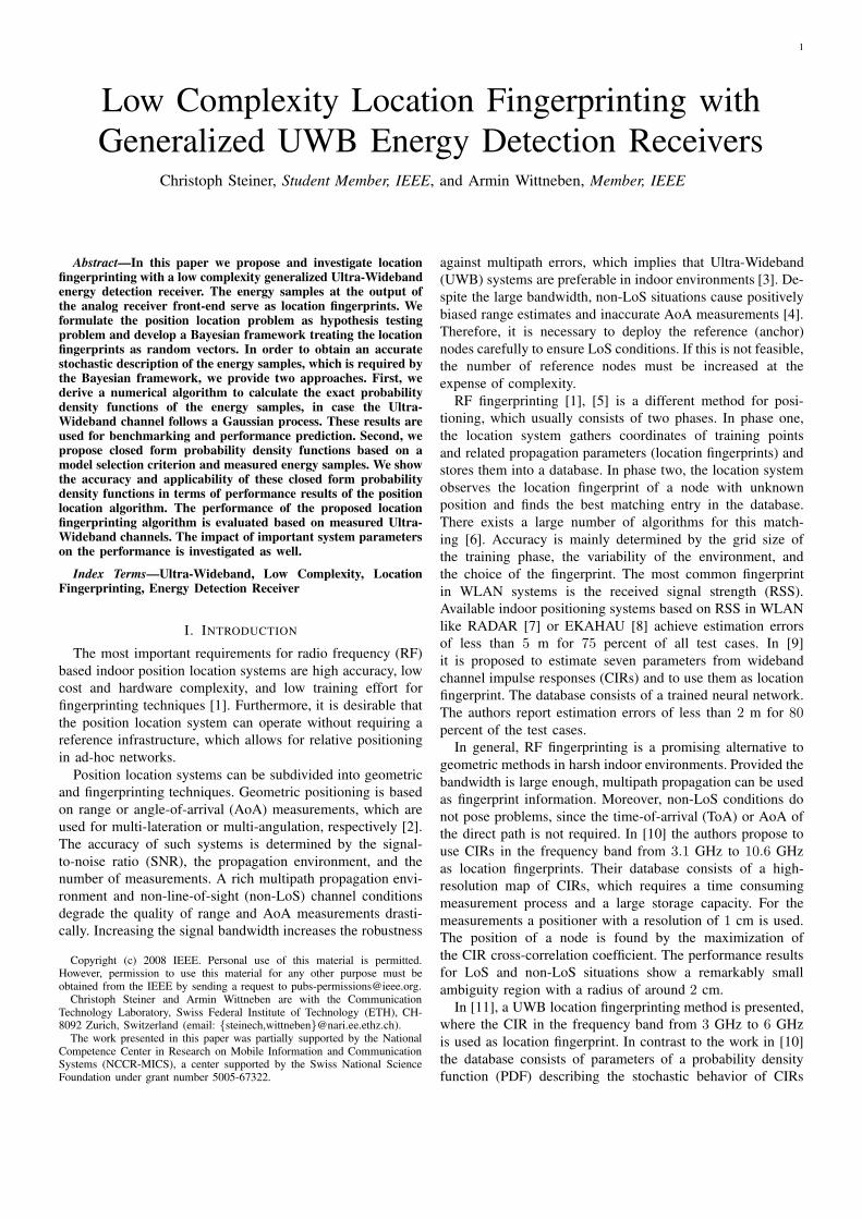
We consider an indoor environment with mobile nodescommunicating wirelessly to a static receiver. We define Mregions in this environment. Figure 1 depicts an exemplaryindoor environment with M = 22 regions, which correspondsto the measurement scenario in [13] used for performanceevaluation in this paper. The location fingerprinting systemshould detect the region, in which a mobile node under test iscurrently located. The positions, dimensions, and number ofthe regions are application specific. The 22 regions in Figure 1do not cover the whole room, which might not be sufficientfor some applications. However, we emphasize that manyapplications like data fusion or geo-routing do not require fullcoverage but merely a clustering of wireless nodes.

The static receiver, labeled with RX in Figure 1, performsthe location fingerprinting. In order to detect the current regionof a node, RX observes the location fingerprint y, whichis related to the physical propagation channel between thisnode and RX. We propose that y can be described by aparameterized PDF, which models the stochastic variations ofthe fingerprints over space and time. The parameters of thisPDF distinguish the regions and must be estimated duringthe training phase. This means that all location fingerprints

3

from nodes located in region m are distributed accordingto the PDF with a parameter set Θm. Thus, the fingerprintdatabase consists of the parameter sets Θ1, . . . , ΘM and thecorresponding coordinates of the regions.

Consequently, the problem of deciding in which region anode is located based on the observation y at RX can be for-mulated as a Bayesian M -ary hypothesis testing problem [14],[15]:

Hm : The node exciting y is located in region m.

The a priori probabilities of the hypotheses are denoted byπ1, . . . , πM . They can be thought of as relative number ofnodes located in each region. The average cost or Bayes riskR is defined as

R =

M∑

i=1

M∑

j=1

πjCi,j

∫

Zi

f (y|Hj) dy, (1)

where f (y|Hj)1 is the conditional PDF of y given Hj , and

Zi defines the part of the observation space of y in which Hi

is chosen. The parameters Ci,j for i 6= j describe the costsfor deciding for Hi when Hj is true. For i = j, Ci,i describethe costs of correct decisions.

Following the presentation in [14] the decision rule mini-mizing (1) is found as

m = argminm=1,2,...,M

M∑

j=1

πjCm,jf (y|Hj) , (2)

where Hm denotes the estimate for the true hypothesis. Settingthe costs of wrong decisions to one (Ci,j = 1 for i 6= j) andof correct decisions to zero (Ci,i = 0) the decision rule in (1)can be simplified to

m = argmaxm=1,2,...,M

πmf (y|Hm) . (3)

This decision rule (3) minimizes the total probability of errorPe given by

Pe =M∑

j=1

πj

M∑

i=1,i6=j

P (Hi|Hj) , (4)

where P (Hi|Hj) denotes the probability of deciding forregion i, when the node is located in region j. Note that ingeneral P (Hi|Hj) 6= P (Hj |Hi). Using P (Hi|Hj) and takingthe distances between the centers of the regions di,j intoaccount, we define the average positioning error de accordingto

de ,

M∑

j=1

πj

M∑

i=1

P (Hi|Hj) di,j . (5)

Note that we can account for the position uncertainty withinone region by assigning non-zero values to di,i. These valuesdetermine the minimal achievable average positioning error(size of ambiguity region), when all conditional error proba-bilities P (Hi|Hj) are zero. In order to minimize the average

1The conditioning on Hj determines the parameter set Θj for the PDF ofthe fingerprints from region j.

positioning error instead of Pe the decision rule in (2) mustbe applied with the costs given by Ci,j = di,j .

In order to apply the decision rules in (2) and (3), we requireexpressions for the conditional PDFs f (y|Hm). The locationfingerprints y are generally governed by complicated physicalpropagation mechanisms, antenna characteristics, additive dis-tortions like thermal noise, and the analog signal processing ofthe receiver front-end. The corresponding modeling problemcan be stated as follows: Find a stochastic description fory with least possible model complexity (number of freeparameters), while still accounting for the relevant locationdependent propagation effects.

In [11], a coherent receiver front-end is analyzed and thefingerprints are considered as sampled CIRs in equivalentbaseband representation. Based on UWB channel modelingliterature (e.g. [16] and [17]) the probability distribution ofthe fingerprints is modeled as multivariate (MV), circularsymmetric, complex Gaussian. Therefore, the parameter setΘm consists of a mean vector and a covariance matrix specificfor region m. We show in [11] that this simple stochasticdescription offers enough modeling accuracy of the locationdependent propagation effects for excellent location finger-printing performance.

However, the central theme in this paper is the ED receiverdescribed in the next section.

B. Generalized ED Receiver

The system model of a generalized ED receiver is depictedin Fig. 2.

PSfrag replacements

p(t) hm(t)r(t)

g(t)

g(−t)∫

(·)2

UWBnode

generalized ED front-endw(t)

hBP (t)y[n]

fed

Figure 2. Communication system with generalized ED receiver.

The transmitter (UWB node) employs either pulse positionmodulation or on-off keying and the receiver uses an analogED front-end with a generalized integration filter g(t). Weassume that the receiver is synchronized to the symbol timingof the transmitter. A low complexity solution for symbolsynchronization with ED receiver is proposed in [18]. Theunmodulated input signal to the squaring device within onesymbol period t ∈ [0, Ts] is given by

r(t) = p(t) ∗ hm(t) ∗ hBP (t) + w(t) ∗ hBP (t), (6)

where p(t) is the transmit pulse, hm(t) is the CIR of a nodelocated in region m and hBP (t) is the impulse responseof the receiver front-end bandpass. The signal w(t) modelsthe distortions of the desired signal and is assumed to be arealization of a white Gaussian process with zero mean andpower spectral density N0/2. We denote the average energyof received pulses for CIRs from region m with Em. Bynormalizing Em to E for each m we remove the path loss

4

information. Accordingly, we define the SNR in dB by

SNR = 10 log10

(

E

N0

)

.

The CIR hm(t) comprises the characteristics of receiverand transmitter antennas. If these characteristics deviate sig-nificantly from an isotropic antenna, the fingerprints depend onthe orientations of the antennas. This effect has to be accountedfor during the training phase by either separate training (pa-rameter estimation) for each orientation or by averaging thefingerprints over all orientations as suggested in [8]. Note thatthe UWB antennas2 used for the channel measurements in [13]are approximately isotropic in the azimuth plane.

The signal after the filter g(t) is sampled with fed producingthe ED output samples y[n]. The sampling rate fed and Ts

specify the number of observed energy samples N = Tsfed persymbol. For N = 1 the only available information for locationfingerprinting is the RSS. We emphasize that this informationis not used in our scheme due to the energy normalization.Increasing fed for a fixed Ts gives a higher spatio-temporalresolution of the UWB multipath propagation channel. Theinfluence of fed on the performance is investigated in Sec-tion VII.

In summary, the location fingerprints y of length N forthe ED receiver are obtained by stacking all samples y[n]for n = 1, . . . , N into one vector. As mentioned above weneed the conditional PDFs f (y|Hm) for m = 1, . . . , M forcalculation of (2) or (3). The stochastic modeling of the outputsamples of ED receivers for random or measured propagationchannels is not covered in literature to the best of the authors’knowledge. An accurate stochastic description is, however,essential for any kind of maximum likelihood operation onthe energy samples. We see two possible approaches to thismodeling problem: A) Take existing and accepted stochasticmodels for the propagation channel and try to come up witha mathematical derivation for the distribution of the energysamples. B) Apply a model selection criterion to measuredenergy samples directly.

In Section III we pick up approach A and provide anumerical algorithm to calculate the theoretic distribution ofthe energy samples based on a channel model. In SectionIV we follow approach B and apply Akaike’s InformationCriterion (AIC) to measured energy samples.

C. System Parameters

If not mentioned otherwise, the system parameters are fixedas follows for the calculation of computer simulation results.The transmit pulse p(t) is assumed to be flat in the desiredfrequency band. The bandpass filter has bandwidth 3 GHzfrom 3 to 6 GHz. The sampling frequency of the receiver isequal to fed = 1 GHz. A symbol period of Ts = 30 ns isconsidered, which leads to N = 30. Continuous-time signalsare represented by samples obtained with fs = 40 GHz.

2Skycross SM3TO10MA [19]

III. EXACT PDF OF ED OUTPUT SAMPLES FOR AGAUSSIAN CHANNEL MODEL

In the following, the exact PDFs f (y[n]|Hm) are calculatedunder the assumption that the channel hm(t) and the distor-tion signal w(t) are realizations of real Gaussian processes.The specific parameters of these Gaussian processes are notrelevant for the theoretical derivation. There are three reasonsto consider a Gaussian channel model: i) There exist analysesof measurement data (e.g. [16] and [17]), which support theGaussian assumption also for UWB channels. ii) This deriva-tion enables performance prediction based on first and secondorder channel statistics without requiring extensive channelmeasurements, because the parameters of the Gaussian channelmodel can be obtained via ray tracing tools or deterministicchannel models. iii) For all other models the mathematicalderivation will most likely fail due to intractability.

We represent the part of the real and band-limited signal r(t)causing y[n] by the vector rn of length I , which is obtainedby sampling r(t) with fs. We assume that rn is a realizationof a MV Gaussian distribution with a mean vector vn,m and acovariance matrix Sn,m. In the following derivation the sampleindex n and the region index m are dropped for notationalconvenience.

The filter g(t) is assumed to be time-limited to the interval[0, 1/fed]. Additionally assuming that g(t) is a real and positivefunction, the energy sample y can be written as positivedefinite Gaussian quadratic form according to

y = rT Gr. (7)

The entries in the diagonal matrix G are obtained by samplingg(−t) for −1/fed ≤ t ≤ 0 with fs. The quadratic form in (7)can be diagonalized according to [20]

y =

I∑

i=1

λiz2i , (8)

such that the PDF of y denoted by f (y) remains the same. Therandom variables zi are independent and Gaussian distributedwith variance one and their means γi are given by

γi =(

S−1/2ui

)T

v,

where λi and ui denote the i-th eigenvalue and eigenvector ofS1/2GS1/2.

If all λi are equal and there exists at least one γi 6= 0,then y is distributed according to a Noncentral Chi-squaredistribution.3 Such a PDF is obtained, when the conditionalPDF of y given a channel realization is sought (e.g. [21]). Notethat this is only valid for rectangular integration windows, i.e.g(t) = constant for 0 ≤ t ≤ 1/fed and zero otherwise.

For arbitrary λi, a closed form expression for f (y) does notexist. Grenander, Pollak, and Slepian present an efficient andnumerically stable approach to calculate f (y) for zero meanrandom variables zi (γi = 0 ∀i) in [22]. We extend this methodto the general case of nonzero means in the following. Thisapproach is based on Fourier’s inversion of the characteristic

3If all γi = 0, then y is distributed according to a Chi-square distribution.

5

function of y, which is for nonzero means and t =√−1ω

given by [23]

Ψy (t) =

I∏

i=1

(1 − 2tλi)−1/2 exp

(

tγ2i λi

1 − 2tλi

)

. (9)

The logarithmic derivative of (9) is given by

∂ln (Ψy (t))

∂t=

∂Ψy (t)

∂t

1

Ψy (t)

=√−1

I∑

i=1

λi

1 − 2tλi+

γ2i λi

(1 − 2tλi)2 . (10)

Applying the inverse Fourier transform to (10) yields anintegral equation for f (y) given by

yf (y) =

∫ y

0

f (y − τ) a (τ) dτ,

where

a (τ) =1

2

(

I∑

i=1

exp(

− τ

2λi

)(

1 +γ2

i τ

2λi

)

)

.

This integral equation can be approximated using the trape-zoidal integration rule according to [22], which yields

f (k∆) =1

k − 12a(0)

k−1∑

l=1

f(l∆)a((k − l)∆),

where ∆ is the mesh size and k = 2, 3, . . .. This recursivealgorithm requires nonzero initial values, which are obtainedby using an analytic approximation to f (y) around y = 0based on Taylor series expansion of (9) and inverse Fouriertransform. The approximation is given by

f (y) =y(I/2)−1exp

(

− 12

∑Ii=1 γ2

i

)

2I/2Γ (I/2)∏I

i=1 λ1/2i

×(

1 +y

2I

I∑

i=1

γ2i − 1

λi+ E

(

y2)

)

,

for small positive values of y. The error term E(

y2)

statesthat all exponents in the error term are larger than or equal to2. This error term is negligible for sufficiently small values ofy.

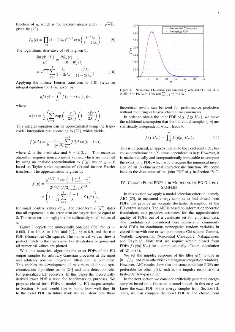
Figure 3 depicts the numerically obtained PDF for ∆ =0.005, I = 10, λi = 1 ∀i, and

∑Ii=1 γ2

i = 6.9, and the truePDF (Noncentral Chi-square). The numerical values show aperfect match to the true curve. For illustration purposes notall numerical values are plotted.

With this numerical algorithm the exact PDFs of the EDoutput samples for arbitrary Gaussian processes at the inputand arbitrary positive integration filters can be computed.This enables the development of maximum likelihood syn-chronization algorithms as in [24] and data detection rulesfor generalized ED receivers. In this paper the theoreticallyderived exact PDF is used for benchmarking purposes. Wepropose closed form PDFs to model the ED output samplesin Section IV and would like to know how well they fitto the exact PDF. In future work we will show how these

0 10 20 30 40 50 60 700

0.01

0.02

0.03

0.04

0.05

0.06

0.07

Noncentral Chi−squareNumerical PDF

PSfrag replacements

y

f(y

)

Figure 3. Noncentral Chi-square and numerically obtained PDF for ∆ =0.005, I = 10, λi = 1 ∀i, and

∑Ii=1

γ2

i = 6.9.

theoretical results can be used for performance predictionwithout requiring extensive channel measurements.

In order to obtain the joint PDF of y, f (y|Hm), we makethe additional assumption that the individual samples y[n] arestatistically independent, which leads to

f (y|Hm) =

N∏

n=1

f (y[n]|Hm) . (11)

This is, in general, an approximation to the exact joint PDF, be-cause correlations in r(t) cause dependencies in y. However, itis mathematically and computationally intractable to computethe exact joint PDF, which would require the numerical inver-sion of an N -dimensional characteristic function. We comeback to the discussion of the joint PDF of y in Section IV-C.

IV. CLOSED FORM PDFS FOR MODELING OF ED OUTPUTSAMPLES

In this section we apply a model selection criterion, namelyAIC [25], to measured energy samples to find closed formPDFs that provide an accurate stochastic description of theED output samples. The AIC is based on information theoreticfoundations and provides estimates for the approximationquality of PDFs out of a candidate set for empirical data.The candidate set considered here consists of commonlyused PDFs for continuous nonnegative random variables inclosed form with one or two parameters: Chi-square, Gamma,Weibull, Log-normal, Noncentral Chi-square, Nakagami-m,and Rayleigh. Note that we require simple closed formPDFs f (y[n]|Hm) for a computationally efficient calculationof (2) or (3).

We set the impulse response of the filter g(t) to one in[0, 1/fed] and zero otherwise (rectangular integration window).However, AIC results show that the same candidate PDFs arepreferable for other g(t), such as the impulse response of afirst-order low-pass filter.

In the next section we consider artificially generated energysamples based on a Gaussian channel model. In this case weknow the exact PDF of the energy samples from Section III.Thus, we can compare the exact PDF to the closed form

6

approximations. In Section IV-B we apply AIC to measuredenergy samples.

A. Gaussian Channel Model

We assume that w(t) and hm(t) are realizations of Gaus-sian processes. The channel parameters (1st and 2nd orderstatistics) are estimated from measured CIRs. Given theseparameters and the SNR, 50000 realizations of r(t) aregenerated. Processing r(t) according to the ED front-end (cf.Figure 2), artificial realizations of the ED output samples y[n]are obtained.

0 5 10 15 20 25 300

0.51

Chi−square

0 5 10 15 20 25 300

0.51

Gamma

0 5 10 15 20 25 300

0.51

Weibull

0 5 10 15 20 25 300

0.51

Log−normal

Aka

ike

wei

ghts

0 5 10 15 20 25 300

0.51

Noncentral Chi−square

0 5 10 15 20 25 300

0.51

Nakagami−m

0 5 10 15 20 25 300

0.51

Rayleigh

PSfrag replacements

nn

Figure 4. Akaike weights at SNR = 10 dB for Gaussian channel model.

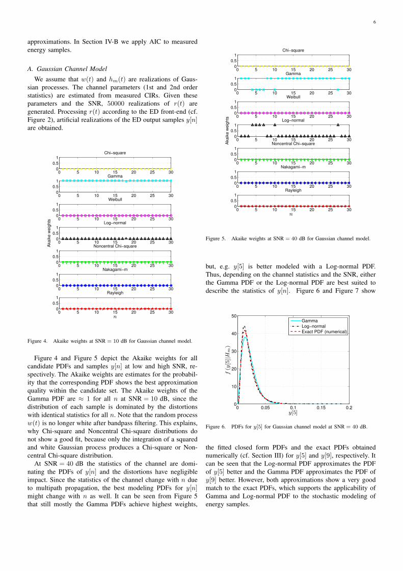
Figure 4 and Figure 5 depict the Akaike weights for allcandidate PDFs and samples y[n] at low and high SNR, re-spectively. The Akaike weights are estimates for the probabil-ity that the corresponding PDF shows the best approximationquality within the candidate set. The Akaike weights of theGamma PDF are ≈ 1 for all n at SNR = 10 dB, since thedistribution of each sample is dominated by the distortionswith identical statistics for all n. Note that the random processw(t) is no longer white after bandpass filtering. This explains,why Chi-square and Noncentral Chi-square distributions donot show a good fit, because only the integration of a squaredand white Gaussian process produces a Chi-square or Non-central Chi-square distribution.

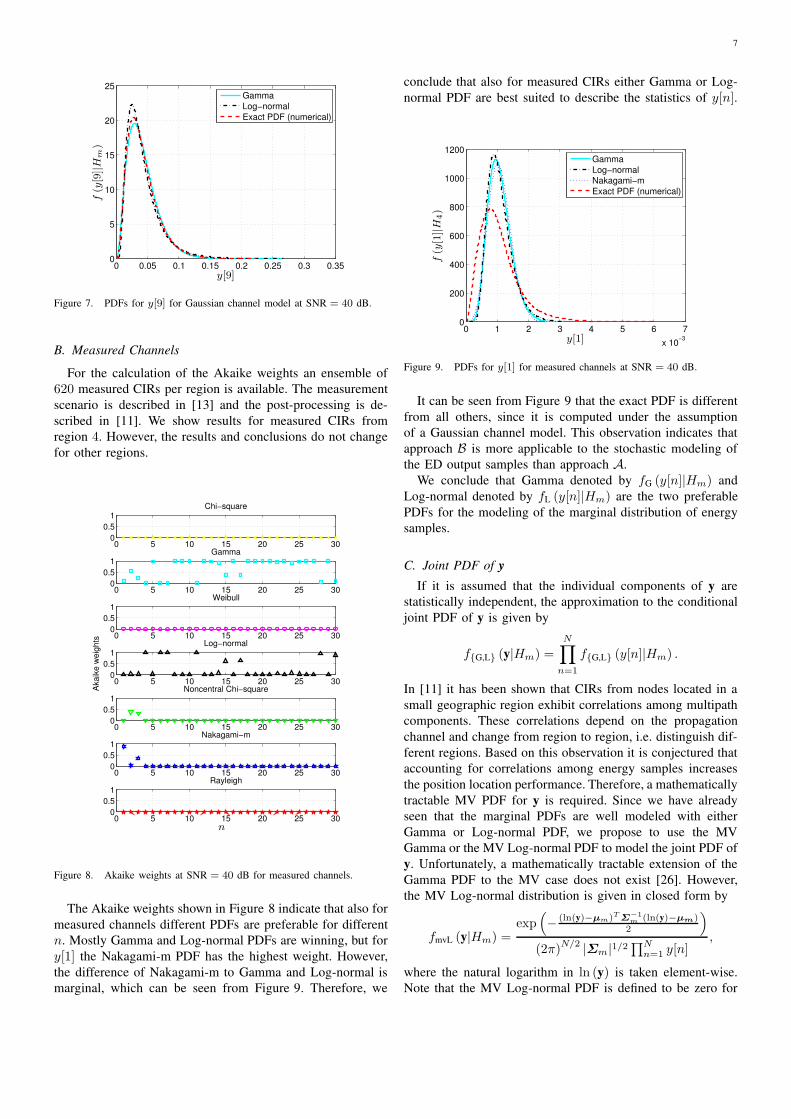
At SNR = 40 dB the statistics of the channel are domi-nating the PDFs of y[n] and the distortions have negligibleimpact. Since the statistics of the channel change with n dueto multipath propagation, the best modeling PDFs for y[n]might change with n as well. It can be seen from Figure 5that still mostly the Gamma PDFs achieve highest weights,

0 5 10 15 20 25 300

0.51

Chi−square

0 5 10 15 20 25 300

0.51

Gamma

0 5 10 15 20 25 300

0.51

Weibull

0 5 10 15 20 25 300

0.51

Log−normal

Aka

ike

wei

ghts

0 5 10 15 20 25 300

0.51

Noncentral Chi−square

0 5 10 15 20 25 300

0.51

Nakagami−m

0 5 10 15 20 25 300

0.51

Rayleigh

PSfrag replacementsn

n

Figure 5. Akaike weights at SNR = 40 dB for Gaussian channel model.

but, e.g. y[5] is better modeled with a Log-normal PDF.Thus, depending on the channel statistics and the SNR, eitherthe Gamma PDF or the Log-normal PDF are best suited todescribe the statistics of y[n]. Figure 6 and Figure 7 show

0 0.05 0.1 0.15 0.20

10

20

30

40

50

GammaLog−normalExact PDF (numerical)

PSfrag replacements

y[5]

f(y

[5]|H

m)

Figure 6. PDFs for y[5] for Gaussian channel model at SNR = 40 dB.

the fitted closed form PDFs and the exact PDFs obtainednumerically (cf. Section III) for y[5] and y[9], respectively. Itcan be seen that the Log-normal PDF approximates the PDFof y[5] better and the Gamma PDF approximates the PDF ofy[9] better. However, both approximations show a very goodmatch to the exact PDFs, which supports the applicability ofGamma and Log-normal PDF to the stochastic modeling ofenergy samples.

7

0 0.05 0.1 0.15 0.2 0.25 0.3 0.350

5

10

15

20

25

GammaLog−normalExact PDF (numerical)

PSfrag replacements

y[9]

f(y

[9]|H

m)

Figure 7. PDFs for y[9] for Gaussian channel model at SNR = 40 dB.

B. Measured Channels

For the calculation of the Akaike weights an ensemble of620 measured CIRs per region is available. The measurementscenario is described in [13] and the post-processing is de-scribed in [11]. We show results for measured CIRs fromregion 4. However, the results and conclusions do not changefor other regions.

0 5 10 15 20 25 300

0.51

Chi−square

0 5 10 15 20 25 300

0.51

Gamma

0 5 10 15 20 25 300

0.51

Weibull

0 5 10 15 20 25 300

0.51

Log−normal

Aka

ike

wei

ghts

0 5 10 15 20 25 300

0.51

Noncentral Chi−square

0 5 10 15 20 25 300

0.51

Nakagami−m

0 5 10 15 20 25 300

0.51

Rayleigh

PSfrag replacements n

Figure 8. Akaike weights at SNR = 40 dB for measured channels.

The Akaike weights shown in Figure 8 indicate that also formeasured channels different PDFs are preferable for differentn. Mostly Gamma and Log-normal PDFs are winning, but fory[1] the Nakagami-m PDF has the highest weight. However,the difference of Nakagami-m to Gamma and Log-normal ismarginal, which can be seen from Figure 9. Therefore, we

conclude that also for measured CIRs either Gamma or Log-normal PDF are best suited to describe the statistics of y[n].

0 1 2 3 4 5 6 7

x 10−3

0

200

400

600

800

1000

1200

GammaLog−normalNakagami−mExact PDF (numerical)

PSfrag replacements

n

y[1]

f(y

[1]|H

4)

Figure 9. PDFs for y[1] for measured channels at SNR = 40 dB.

It can be seen from Figure 9 that the exact PDF is differentfrom all others, since it is computed under the assumptionof a Gaussian channel model. This observation indicates thatapproach B is more applicable to the stochastic modeling ofthe ED output samples than approach A.

We conclude that Gamma denoted by fG (y[n]|Hm) andLog-normal denoted by fL (y[n]|Hm) are the two preferablePDFs for the modeling of the marginal distribution of energysamples.

C. Joint PDF of yIf it is assumed that the individual components of y are

statistically independent, the approximation to the conditionaljoint PDF of y is given by

f{G,L} (y|Hm) =N∏

n=1

f{G,L} (y[n]|Hm) .

In [11] it has been shown that CIRs from nodes located in asmall geographic region exhibit correlations among multipathcomponents. These correlations depend on the propagationchannel and change from region to region, i.e. distinguish dif-ferent regions. Based on this observation it is conjectured thataccounting for correlations among energy samples increasesthe position location performance. Therefore, a mathematicallytractable MV PDF for y is required. Since we have alreadyseen that the marginal PDFs are well modeled with eitherGamma or Log-normal PDF, we propose to use the MVGamma or the MV Log-normal PDF to model the joint PDF ofy. Unfortunately, a mathematically tractable extension of theGamma PDF to the MV case does not exist [26]. However,the MV Log-normal distribution is given in closed form by

fmvL (y|Hm) =exp

(

− (ln(y)−µm)T Σ−1

m(ln(y)−µm)

2

)

(2π)N/2 |Σm|1/2∏N

n=1 y[n],

where the natural logarithm in ln (y) is taken element-wise.Note that the MV Log-normal PDF is defined to be zero for

8

y ≤ 0. The random variable transformation x = ln (y) rendersthe random vector x as jointly Gaussian distributed with meanvector µm and covariance matrix Σm.

V. POSITION LOCATION SYSTEM

A. Parameter Estimation during the Training Phase

For the calculation of (2) or (3) during the localizationphase, the parameters of the conditional PDFs given hy-potheses Hm for all m must be estimated during the train-ing phase. The maximum likelihood parameter estimates forfG (y[n]|Hm) based on L training samples {y[n]1, . . . , y[n]L}from nodes located in region m are given by [27]

ln (αn,m) − Γ′

(αn,m)

Γ (αn,m)

= ln

(

1

L

L∑

l=1

y[n]l

)

− 1

L

L∑

l=1

ln (y[n]l) , (12)

βn,m =1

αn,mL

L∑

l=1

y[n]l. (13)

Although there exists no closed form solution for αn,m in (12),numerical solvers can be applied. The maximum likelihoodparameter estimates for fmvL (y|Hm) are given by [26]

µm =1

L

L∑

l=1

ln (yl)

Σm =1

L

L∑

l=1

(ln (yl) − µm) (ln (yl) − µm)T

.

We notice that there are 2N free real parameters to estimateif it is assumed that the energy samples are independent. Ifwe model also the correlation among energy samples thereare N + N(N + 1)/2 free real parameters to estimate. Theaccuracy of the parameter estimates is determined by L. Asa rule of thumb, L should be approximately as large asthe number of free real parameters for a precise stochasticdescription. Thus, there is a trade-off between training effortand performance. We investigate the impact of L on theperformance in Section VII.

The proposed location fingerprinting framework enables thecombination of training and localization phase via iterative al-gorithms, which improve the quality of the parameter estimatesduring the localization phase. For example, the application ofthe expectation maximization algorithm is proposed in [28].

B. Localization Phase with Multiple Observations

In a realistic localization scenario it is conceivable that RXhas multiple independent observations from the device undertest available for the localization (region detection). If thetransmitting node is equipped with multiple antennas it canuse them sequentially to transmit signals to the receiver. Ifthe node is mobile it can transmit periodically always from aslightly different position. These are just two examples howmultiple independent observations within one region could begenerated. In the following we derive the optimal decision ruletaking multiple observations into account.

Let us assume the receiver has recorded K observations{y1, . . . , yK}. We further assume that these observations areindependent and are caused by a transmitter located in oneregion. We stack all observations into one big vector y =[

yT1 , . . . , yT

K

]T and note that the PDF of this big vector iscomposed out of the individual PDFs for yk. Assuming theMV Log-normal model and conditioned on hypothesis Hm

this results in fmvL (y|Hm) =∏K

k=1 fmvL (yk|Hm), whichfollows from the independence of the individual observations.By inserting the PDFs for y given Hm into (3) we obtain afteralgebraic manipulations the following decision rule:

m = argmaxm=1,2,...,M

ln

(

πm

|Σm|K/2

)

−

1

2

K∑

k=1

(ln (yk) − µm)T

Σ−1m (ln (yk) − µm) .

The performance of this decision rule increases with increasingK due to the additional available information. A similar effectcan be observed, when for example repetition coding is usedfor data transmission. Moreover, channel estimation algorithmsexploit multiple observations for performance enhancement aswell.

VI. ACCURACY AND APPLICABILITY OF CLOSED FORMPDFS

In Section IV we have seen by visual inspection that theproposed closed form PDFs are good approximations to theexact PDF for a Gaussian channel model. In this section weconfirm this observation by analyzing Pe. For this analysis it issufficient to restrict the number of hypotheses to two (M = 2).Let us consider H5 and H10 with π5 = π10 = 0.5. We presentresults assuming a Gaussian channel model as well as formeasured channels. The parameters of the Gaussian channelmodel are estimated using 620 measured CIRs from each re-gion. Based on these parameters the exact PDFs are calculated.The parameters of the closed form PDFs are estimated basedon L = 400 training vectors per region.

10 20 30 40 5010

−2

10−1

100

SNR [dB]

Pe

Exact PDFMV Log−normal PDFGamma PDFLog−normal PDF

Dependent ED samples

Independent ED samples

Figure 10. Pe for H5 and H10 with π5 = π10 = 0.5 for Gaussian channelmodel.

Figure 10 depicts Pe for artificially generated CIRs basedon the Gaussian channel model. The components of y are

9

in general dependent due to correlations in r(t). In order toobtain independent components the Gaussian channel modelis modified, such that the covariance matrices between vectorsri and rj for i 6= j are zero matrices. This is done to emulatea situation, where the decision rule in (3) using the exact PDFin (11) is optimal. The corresponding performance curves canbe seen in Figure 10 marked with independent ED samples.It can be seen that all closed form PDFs achieve Pe close tothe optimum, at which the Gamma PDF comes closest. Theseresults support the accuracy and applicability of the proposedclosed form PDFs.

The unmodified Gaussian channel model causes dependen-cies in y. The corresponding curves are marked with dependentED samples. There is a performance loss due to the wrongindependence assumption. Note that (11) does not provide theoptimal performance anymore. Only the MV Log-normal PDFaccounts for correlations among energy samples. However, itcan be seen that for the Gaussian channel model the achievableperformance improvement compared to the PDFs assumingindependent energy samples is only marginal.

10 20 30 40 5010

−4

10−3

10−2

10−1

100

SNR [dB]

Pe

Gamma PDFLog−normal PDFMV Log−normal PDFExact PDFCoherent RX

Figure 11. Pe for H5 and H10 with π5 = π10 = 0.5 for measured channels.

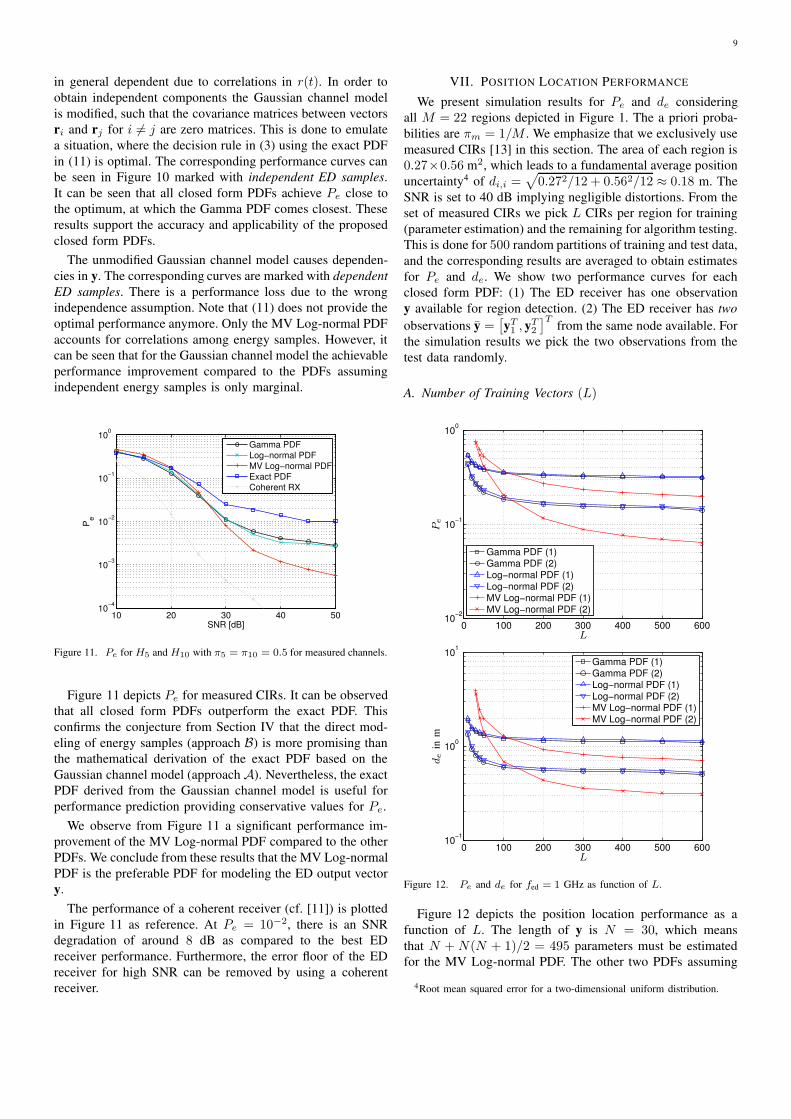
Figure 11 depicts Pe for measured CIRs. It can be observedthat all closed form PDFs outperform the exact PDF. Thisconfirms the conjecture from Section IV that the direct mod-eling of energy samples (approach B) is more promising thanthe mathematical derivation of the exact PDF based on theGaussian channel model (approach A). Nevertheless, the exactPDF derived from the Gaussian channel model is useful forperformance prediction providing conservative values for Pe.

We observe from Figure 11 a significant performance im-provement of the MV Log-normal PDF compared to the otherPDFs. We conclude from these results that the MV Log-normalPDF is the preferable PDF for modeling the ED output vectory.

The performance of a coherent receiver (cf. [11]) is plottedin Figure 11 as reference. At Pe = 10−2, there is an SNRdegradation of around 8 dB as compared to the best EDreceiver performance. Furthermore, the error floor of the EDreceiver for high SNR can be removed by using a coherentreceiver.

VII. POSITION LOCATION PERFORMANCE

We present simulation results for Pe and de consideringall M = 22 regions depicted in Figure 1. The a priori proba-bilities are πm = 1/M . We emphasize that we exclusively usemeasured CIRs [13] in this section. The area of each region is0.27×0.56 m2, which leads to a fundamental average positionuncertainty4 of di,i =

√

0.272/12 + 0.562/12 ≈ 0.18 m. TheSNR is set to 40 dB implying negligible distortions. From theset of measured CIRs we pick L CIRs per region for training(parameter estimation) and the remaining for algorithm testing.This is done for 500 random partitions of training and test data,and the corresponding results are averaged to obtain estimatesfor Pe and de. We show two performance curves for eachclosed form PDF: (1) The ED receiver has one observationy available for region detection. (2) The ED receiver has twoobservations y =

[

yT1 , yT

2

]T from the same node available. Forthe simulation results we pick the two observations from thetest data randomly.

A. Number of Training Vectors (L)

0 100 200 300 400 500 60010

−2

10−1

100

Gamma PDF (1)Gamma PDF (2)Log−normal PDF (1)Log−normal PDF (2)MV Log−normal PDF (1)MV Log−normal PDF (2)

PSfrag replacements

de in m

Pe

L

0 100 200 300 400 500 60010

−1

100

101

Gamma PDF (1)Gamma PDF (2)Log−normal PDF (1)Log−normal PDF (2)MV Log−normal PDF (1)MV Log−normal PDF (2)

PSfrag replacements

de

inm

Pe

L

Figure 12. Pe and de for fed = 1 GHz as function of L.

Figure 12 depicts the position location performance as afunction of L. The length of y is N = 30, which meansthat N + N(N + 1)/2 = 495 parameters must be estimatedfor the MV Log-normal PDF. The other two PDFs assuming

4Root mean squared error for a two-dimensional uniform distribution.

10

independent taps require the estimation of 2N = 60 parame-ters. Therefore, the performance of the MV Log-normal PDFdrops drastically for small L, since the stochastic descriptionbecomes unreliable. However, for L > 100 the higher modelcomplexity of MV Log-normal pays off. Further, it can beobserved that two observations give a significant performanceimprovement. The average positioning error using the MVLog-normal model can be decreased from 93 cm to 43 cmat L = 200.

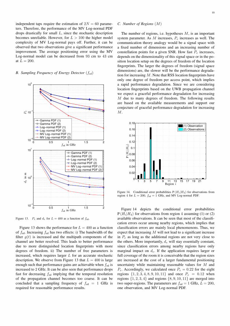
B. Sampling Frequency of Energy Detector (fed)

0 0.5 1 1.5 210

−2

10−1

100

Gamma PDF (1)Gamma PDF (2)Log−normal PDF (1)Log−normal PDF (2)MV Log−normal PDF (1)MV Log−normal PDF (2)

PSfrag replacements

de in m

Pe

fed in GHz

0 0.5 1 1.5 210

−1

100

101

Gamma PDF (1)Gamma PDF (2)Log−normal PDF (1)Log−normal PDF (2)MV Log−normal PDF (1)MV Log−normal PDF (2)

PSfrag replacements

de

inm

Pe

fed in GHz

Figure 13. Pe and de for L = 400 as a function of fed.

Figure 13 shows the performance for L = 400 as a functionof fed. Increasing fed has two effects: i) The bandwidth of thefilter g(t) is increased and the multipath components of thechannel are better resolved. This leads to better performancedue to more distinguished location fingerprints with moredegrees of freedom. ii) The number of free parameters isincreased, which requires larger L for an accurate stochasticdescription. We observe from Figure 13 that L = 400 is largeenough such that performance gains are achievable when fed isincreased to 2 GHz. It can be also seen that performance dropsfast for decreasing fed implying that the temporal resolutionof the propagation channel becomes too coarse. It can beconcluded that a sampling frequency of fed = 1 GHz isrequired for reasonable performance results.

C. Number of Regions (M)

The number of regions, i.e. hypotheses M , is an importantsystem parameter. As M increases, Pe increases as well. Thecommunication theory analogy would be a signal space witha fixed number of dimensions and an increasing number ofconstellation points for a given SNR. How fast Pe increases,depends on the dimensionality of this signal space or in the po-sition location setup on the degrees of freedom of the locationfingerprints. The larger the degrees of freedom (signal spacedimensions) are, the slower will be the performance degrada-tion for increasing M . Note that RSS location fingerprints haveonly one degree of freedom per access point, which impliesa rapid performance degradation. Since we are consideringlocation fingerprints based on the UWB propagation channelwe expect a graceful performance degradation for increasingM due to many degrees of freedom. The following resultsare based on the available measurements and support ourconjecture of graceful performance degradation for increasingM .

1 3 5 7 9 11 13 15 17 19 210

0.02

0.04

0.06

0.08

0.1

0.12

0.14

0.16

0.18

(1) Observation(2) Observations

PSfrag replacements

Region i

P(H

i|H

4)

Figure 14. Conditional error probabilities P (Hi|H4) for observations fromregion 4 for L = 200, fed = 1 GHz, and MV Log-normal PDF.

Figure 14 depicts the conditional error probabilitiesP (Hi|H4) for observations from region 4 assuming (1) or (2)available observations. It can be seen that most of the classifi-cation errors occur among nearby regions, which implies thatclassification errors are mainly local phenomenons. Thus, weexpect that increasing M will not lead to a significant increasein Pe as long as the additional regions are not very close tothe others. More importantly, de will stay essentially constant,since classification errors among nearby regions have onlymarginal impact on de. If the application requires larger orfull coverage of the room it is conceivable that the region sizesare increased at the cost of a larger fundamental positioninguncertainty while maintaining reasonable values for M andPe. Accordingly, we calculated once Pe = 0.22 for the eightregions {1, 2, 3, 4, 8, 9, 10, 11} and once Pe = 0.12 whenregions {1, 2, 3, 4} and regions {8, 9, 10, 11} are merged intotwo super-regions. The parameters are fed = 1 GHz, L = 200,one observation, and MV Log-normal PDF.

11

D. Summary

In summary we can achieve an average positioning error ofde ≈ 93 cm for a high SNR of 40 dB, fed = 1 GHz, L = 200,and M = 22 with a single observation of the output samplesof a generalized ED receiver. If two observations are used theerror decreases to de ≈ 43 cm. Note that this performanceis achieved with a single ED receiver and by modeling theenergy samples with a MV Log-normal PDF.

If the distortions are non-negligible (low SNR) the cor-responding performance degradation can be compensated byusing more observations for the region detection process. Notethat in this case the node need not be mobile, because thedistortions change from observation to observation.

VIII. CONCLUSIONS AND FUTURE WORK

This paper presents the first investigation of location fin-gerprinting with a generalized UWB ED receiver. The mainpurpose of this paper is to show that and how location fin-gerprinting with such a low complexity receiver structure canbe done and that a reasonable performance is achievable. Wevalidate the proposed position location system with measuredUWB channels. These measurements include uncontrolledtime variations of the channel caused by moving people whichhave been present during the measurements. Therefore, we areconfident that the performance results presented in Section VIIare close to reality. However, there are still open items untilsuch a position location system can be implemented anddeployed.

First, the impact of antenna patterns on the location fin-gerprints has to be investigated. Since the proposed positionlocation method does not rely on path loss information butrather on the temporal structure of the multipath channel, weassume that the location fingerprints are robust to varyingantenna patterns. Note that the antenna characteristics influ-ence only the amplitude and not the delay of the multipathcomponents.

Second, time-varying propagation channels have to be stud-ied in more detail. We conjecture that random distortions of thefingerprints like moving objects can be absorbed into the dis-tortion signal w(t). By increasing the number of observationsthe envisioned performance required by the application can besustained. However, we also conjecture that major changes ofthe propagation environment like relocation of large objectswould require adaptation of the stochastic description. Sincesuch changes might not happen very frequently a new trainingphase is conceivable. Moreover, iterative algorithms might beable to track such changes without requiring a new trainingphase.

Third, the impact of increasing M on the position locationaccuracy needs to be further analyzed. As a first step, weprovide performance results in Section VII-C, which supportthe expectation that the position location accuracy does notdegrade drastically as M grows. Beyond that, the proposedtheoretical framework enables a conservative performanceprediction without requiring measurements by applying theGaussian channel model. Using for example ray-tracing toolsit is possible to calculate the mean and the covariance matrix

of CIRs within one region efficiently. In this way a whole roomcan be covered and the impact of varying M and region dimen-sions can be studied. Such a theoretical performance analysisand performance results based on additional measurements areplanned for future work.

REFERENCES

[1] K. Kaemarungsi, “Design of indoor positioning systems based onlocation fingerprinting technique,” Ph.D. Thesis, Univ. of Pittsburgh,2005.

[2] S. Gezici, Z. Tian, G. Giannakis, H. Kobayashi, A. Molisch, H. Poor, andZ. Sahinoglu, “Localization via Ultra-Wideband radios,” IEEE SignalProcessing Magazine, vol. 22, no. 4, pp. 70–84, July 2005.

[3] J.-Y. Lee and R. A. Scholtz, “Ranging in a dense multipath environ-ment using an UWB radio link,” IEEE Journal on Selected Areas inCommunications, vol. 20, no. 9, pp. 1677–1683, Dec. 2002.

[4] Y. Qi, H. Kobayashi, and H. Suda, “Analysis of wireless geolocationin a non-line-of-sight environment,” IEEE Transactions on WirelessCommunications, vol. 5, no. 3, pp. 672–681, March 2006.

[5] F. Gustafsson and F. Gunnarsson, “Mobile positioning using wirelessnetworks: possibilities and fundamental limitations based on availablewireless network measurements,” IEEE Signal Processing Magazine,vol. 22, no. 4, pp. 41–53, 2005.

[6] M. Brunato and R. Battiti, “Statistical learning theory for locationfingerprinting in wireless LANs,” Comput. Netw. ISDN Syst., vol. 47,no. 6, pp. 825–845, 2005.

[7] P. Bahl and V. N. Padmanabhan, “RADAR: An in-building RF-baseduser location and tracking system,” in Proceedings of IEEE INFOCOM,Tel Aviv, Israel, Mar. 2000, pp. 775–784.

[8] “Ekahau positioning engine,” Ekahau Inc. [Online]. Available:http://www.ekahau.com

[9] C. Nerguizian, C. Despins, and S. Affes, “Geolocation in mines with animpulse response fingerprinting technique and neural networks,” IEEETransactions on Wireless Communications, vol. 5, no. 3, pp. 603–611,Mar. 2006.

[10] W. Malik and B. Allen, “Wireless sensor positioning with ultrawidebandfingerprinting,” First European Conference on Antennas and Propaga-tion, EuCAP 2006, p. 5, Nov. 2006.

[11] C. Steiner, F. Althaus, F. Troesch, and A. Wittneben, “Ultra-WidebandGeo-Regioning: A Novel Clustering and Localization Technique,”EURASIP Journal on Advances in Signal Processing, Special Issue onSignal Processing for Location Estimation and Tracking in WirelessEnvironments, Nov. 2007.

[12] F. Troesch, C. Steiner, T. Zasowski, T. Burger, and A. Wittneben, “Hard-ware aware optimization of an ultra low power UWB communicationsystem,” IEEE International Conference on Ultra-Wideband, ICUWB2007, pp. 174–179, September 2007.

[13] F. Althaus, F. Troesch, T. Zasowski, and A. Wittneben, “STS measure-ments and characterization,” PULSERS Deliverable D3b6a, vol. IST-2001-32710 PULSERS, 2005.

[14] S. M. Kay, Fundamentals of Statistical Signal Processing, Volume 2:Detection Theory. Prentice Hall PTR, January 1998.

[15] H. van Trees, Detection, Estimation, and Modulation Theory. Wiley,New York, 1968, part I.

[16] U. G. Schuster and H. Bolcskei, “Ultrawideband channel modelingon the basis of information-theoretic criteria,” IEEE Transactions onWireless Communications, vol. 6, no. 7, pp. 2464–2475, Jul. 2007,originally submitted to JSAC, accepted for publication, but withdrawnbecause of a severe constraint on the overall length of the finalpaper. Resubmitted to TWireless with many modifications. [Online].Available: http://www.nari.ee.ethz.ch/commth/pubs/p/schuster07-07a

[17] U. G. Schuster, “Wireless communication over wide-band channels,” Ph.D. dissertation, Series in Communica-tion Theory, ISSN 1865-6765, 2009. [Online]. Available:http://www.nari.ee.ethz.ch/commth/pubs/p/schuster09-03a

[18] H. Luecken, T. Zasowski, and A. Wittneben, “Synchronization schemefor low duty cycle UWB impulse radio receiver,” in IEEE InternationalSymposium on Wireless Communication Systems 2008, ISWCS 2008,Oct. 2008, pp. 503–507.

[19] “SM3TO10MA data sheet,” Skycross. [Online]. Available:http://www.skycross.com/Products/PDFs/SMT-3TO10M-A.pdf

[20] G. Tziritas, “On the distribution of positive-definite gaussian quadraticforms,” IEEE Transactions on Information Theory, vol. 33, no. 6, pp.895–906, Nov 1987.

12

[21] A. D’Amico, U. Mengali, and E. Arias-de Reyna, “Energy-detectionUWB receivers with multiple energy measurements,” IEEE Transactionson Wireless Communications, vol. 6, no. 7, pp. 2652–2659, July 2007.

[22] U. Grenander, H. O. Pollak, and D. Slepian, “The distribution ofquadratic forms in normal variates: A small sample theory with ap-plications to spectral analysis,” Journal of the Society for Industrial andApplied Mathematics, vol. 7, no. 4, pp. 374–401, 1959.

[23] G. L. Turin, “The characteristic function of Hermitian quadratic formsin complex normal variables,” Biometrika, vol. 47, no. 1-2, pp. 199–201,1960.

[24] H. Luecken, C. Steiner, and A. Wittneben, “ML timing estimation forgeneralized UWB-IR energy detection receivers,” in IEEE InternationalConference on Ultra-Wideband, ICUWB 2009, Sep. 2009.

[25] H. Akaike, “Information theory and an extension of the maximumlikelihood principle,” Breakthroughs in Statistics, S. Kotz and N.L.Johnson, Eds. New York, U.S.A.: Springer, vol. 1, pp. 610–624, 1992.

[26] S. Kotz, N. Balakrishnan, and N. L. Johnson, Continuous MultivariateDistributions, Models and Applications, 2nd ed. Wiley, 2000, vol. 1.

[27] N. L. Johnson, S. Kotz, and N. Balakrishnan, Continuous UnivariateDistributions, 2nd ed. Wiley, 1994, vol. 1.

[28] C. Steiner and A. Wittneben, “Clustering of wireless sensors based onUltra-Wideband Geo-Regioning,” in Asilomar Conference on Signals,Systems, and Computers, Nov. 2007.

Christoph Steiner received the Dipl.-Ing. degreein Telematics from Graz University of Technol-ogy, Austria, in April 2005 with distinction. SinceSeptember 2005 he is conducting a Ph.D. programat the Swiss Federal Institute of Technology inZurich (ETHZ) at the Communication TechnologyLaboratory. His research interests are in the fieldof signal processing for Ultra-Wideband wirelesscommunication and localization.

Armin Wittneben received the Dipl.-Ing. and theDr.-Ing. (PhD) degree in Electrical Engineering fromthe Technical University of Darmstadt in 1983 and1989 respectively. From 1989 to 1998 he was withthe research organization of ASCOM/Switzerlandand in charge of the Radio Communications researchdepartment. In 1997 he completed the habilitationthesis Diversity schemes in mobile communications.In 1998 he accepted a position as Full Professor ofCommunications at the Saarland University, Saar-brcken (Germany). Since 2002 he has been Full

Professor of Wireless Communications at ETH Zurich and head of theCommunication Technology Laboratory. His research interests comprise thePhysical and the Data Link Layer of Wireless Communication Systems aswell as selected aspects of the Network Layer. Currently he is focusing on(i) cooperative signaling, signal processing and relaying in short range andcellular wireless systems, (ii) Ultra Wideband/Ultra Low Power Wireless, (iii)nonlinear MIMO and (iv) blind position location.