lotterysampling: a novel algorithm for the heavy hitters
TRANSCRIPT

LotterySampling: A Novel Algorithm for the
Heavy Hitters and the Top-k Problems on Data
Streams
Gonzalo Solera Pardo
Thesis director: Conrado Martınez
September 2018
1
Contents
1 Introduction 41.1 Context and stakeholders . . . . . . . . . . . . . . . . . . . . . . 41.2 Problem formulation . . . . . . . . . . . . . . . . . . . . . . . . . 51.3 State of the art . . . . . . . . . . . . . . . . . . . . . . . . . . . . 6
1.3.1 Counter-based algorithms . . . . . . . . . . . . . . . . . . 71.3.2 Sketch-based algorithms . . . . . . . . . . . . . . . . . . . 8
2 Metrics 92.1 Recall and precision . . . . . . . . . . . . . . . . . . . . . . . . . 92.2 Weighted recall . . . . . . . . . . . . . . . . . . . . . . . . . . . . 102.3 Squared error . . . . . . . . . . . . . . . . . . . . . . . . . . . . . 11
3 The algorithms 113.1 BasicLotterySampling . . . . . . . . . . . . . . . . . . . . . . . . . 11
3.1.1 Analysis . . . . . . . . . . . . . . . . . . . . . . . . . . . . 133.1.2 Asymptotic cost . . . . . . . . . . . . . . . . . . . . . . . 16
3.2 ParallelLotterySampling . . . . . . . . . . . . . . . . . . . . . . . . 173.2.1 Asymptotic cost . . . . . . . . . . . . . . . . . . . . . . . 21
3.3 SpaceSavingThreshold . . . . . . . . . . . . . . . . . . . . . . . . . 213.3.1 Asymptotic cost . . . . . . . . . . . . . . . . . . . . . . . 25
3.4 LotterySampling . . . . . . . . . . . . . . . . . . . . . . . . . . . . 253.4.1 Asymptotic cost . . . . . . . . . . . . . . . . . . . . . . . 27
3.5 Other variations . . . . . . . . . . . . . . . . . . . . . . . . . . . 273.5.1 LotterySampling with ticket scaling . . . . . . . . . . . . . 273.5.2 BasicLotterySampling with ticket aging . . . . . . . . . . . 273.5.3 LotterySampling adapted for the weighted setups . . . . . 283.5.4 LotterySampling adapted for the Heavy Hitters problem . 28
4 Implementation 294.1 Project structure . . . . . . . . . . . . . . . . . . . . . . . . . . . 294.2 Implementation details . . . . . . . . . . . . . . . . . . . . . . . . 304.3 Test environment . . . . . . . . . . . . . . . . . . . . . . . . . . . 32
5 Experimentation 325.1 Streams . . . . . . . . . . . . . . . . . . . . . . . . . . . . . . . . 325.2 Experiments . . . . . . . . . . . . . . . . . . . . . . . . . . . . . . 34
6 Conclusions 47
Appendices 48
A Visual inspection of the algorithms’ accuracy 48
2
B Scope and methodology 50B.1 Scope . . . . . . . . . . . . . . . . . . . . . . . . . . . . . . . . . 50B.2 Expected challenges . . . . . . . . . . . . . . . . . . . . . . . . . 51B.3 Methodology . . . . . . . . . . . . . . . . . . . . . . . . . . . . . 51
C Project planning 52C.1 Tasks description and estimated time . . . . . . . . . . . . . . . . 52C.2 Action plan . . . . . . . . . . . . . . . . . . . . . . . . . . . . . . 53
C.2.1 Changes in the planning . . . . . . . . . . . . . . . . . . . 53
D Budget and sustainability 55D.1 Environmental impact . . . . . . . . . . . . . . . . . . . . . . . . 55D.2 Economic impact . . . . . . . . . . . . . . . . . . . . . . . . . . . 56D.3 Social impact . . . . . . . . . . . . . . . . . . . . . . . . . . . . . 57
3

1 Introduction
1.1 Context and stakeholders
The rapid growth of data volume during the last decades has increased theimportance of designing efficient data mining algorithms. In particular, the al-gorithms that operate with massive data streams need to be specially fast andmemory efficient to handle the current requirements of the industry.
In this project, new efficient and accurate algorithms are presented that op-erate on very long streams over a large cardinality set of distinct elements.
This kind of data streams can be found very frequently in network trafficcontexts. For example, the IP addresses of the packets sent through a routerform a large data stream. This stream is composed by a very large cardinalityset of addresses (2128). It’s usually interesting to perform a real-time analysisof those IP addresses to detect anomalies, prevent DDoS attacks or simply toanalyze the kind of traffic that is currently flowing through the router. On thesesituations, the information of which elements (IP addresses) sent throughthe stream are the most frequent is essential. In the DDoS example, thisinformation will help to identify who the attackers are since their IP addresseswill appear many more times than the rest of addresses.
Another case in which that same question has special relevance is in Internetservices that operate at big scale. For example, companies like Google or Ama-zon tend to create region based caches of the most popular content, so that thelatency that their users experience when accessing to it decreases. To achieve it,they perform analysis of the current trends to find popular queries or products.We can then model the sequence of queries or products as a data stream, whichalso has a very large cardinality of distinct elements (all the possible queriesor all the products in the catalog). These companies want to find the frequentelements efficiently and accurately. However, this is not as trivial as it maysound in such big streams, and a trade-off between the two is needed.
The reasons of why such a “simple” problem is not trivial are related tomemory and time constraints. The naıve approach would consist in keeping acounter for each distinct element that is sent through the stream and increasingit for each apparition. However, due to the large cardinalities of the streams,keeping that quantity of counters in memory is unfeasible (because of the mem-ory limitations of the devices) or it’s too costly. Also, in these examples time iscrucial and we can only allow ourselves to spend a few milliseconds of compu-tation for each element sent through the stream.
As the reader can imagine, there is a big and diverse amount of use casesin which this kind of queries about a data stream are relevant. Apart from theprevious examples, domains like telecommunications, Internet advertising, high-
4
performing databases, stock trading platforms or logging systems are speciallyinterested in data mining techniques were some information can be extractedfrom the stream, without the need of storing it in memory, which is totallyunfeasible. On all those cases, data mining algorithms like the ones we proposehave significant interest nowadays.
1.2 Problem formulation
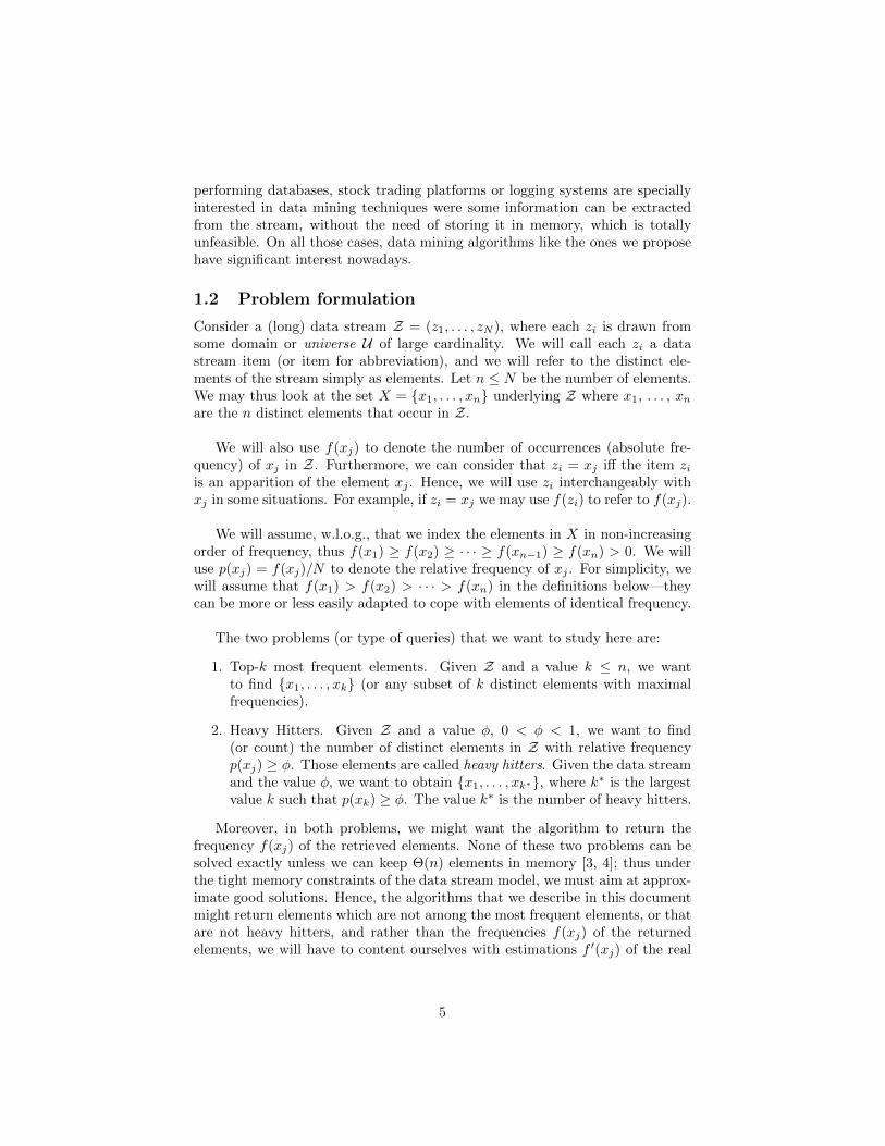
Consider a (long) data stream Z = (z1, . . . , zN ), where each zi is drawn fromsome domain or universe U of large cardinality. We will call each zi a datastream item (or item for abbreviation), and we will refer to the distinct ele-ments of the stream simply as elements. Let n ≤ N be the number of elements.We may thus look at the set X = {x1, . . . , xn} underlying Z where x1, . . . , xnare the n distinct elements that occur in Z.
We will also use f(xj) to denote the number of occurrences (absolute fre-quency) of xj in Z. Furthermore, we can consider that zi = xj iff the item ziis an apparition of the element xj . Hence, we will use zi interchangeably withxj in some situations. For example, if zi = xj we may use f(zi) to refer to f(xj).
We will assume, w.l.o.g., that we index the elements in X in non-increasingorder of frequency, thus f(x1) ≥ f(x2) ≥ · · · ≥ f(xn−1) ≥ f(xn) > 0. We willuse p(xj) = f(xj)/N to denote the relative frequency of xj . For simplicity, wewill assume that f(x1) > f(x2) > · · · > f(xn) in the definitions below—theycan be more or less easily adapted to cope with elements of identical frequency.
The two problems (or type of queries) that we want to study here are:
1. Top-k most frequent elements. Given Z and a value k ≤ n, we wantto find {x1, . . . , xk} (or any subset of k distinct elements with maximalfrequencies).
2. Heavy Hitters. Given Z and a value φ, 0 < φ < 1, we want to find(or count) the number of distinct elements in Z with relative frequencyp(xj) ≥ φ. Those elements are called heavy hitters. Given the data streamand the value φ, we want to obtain {x1, . . . , xk∗}, where k∗ is the largestvalue k such that p(xk) ≥ φ. The value k∗ is the number of heavy hitters.
Moreover, in both problems, we might want the algorithm to return thefrequency f(xj) of the retrieved elements. None of these two problems can besolved exactly unless we can keep Θ(n) elements in memory [3, 4]; thus underthe tight memory constraints of the data stream model, we must aim at approx-imate good solutions. Hence, the algorithms that we describe in this documentmight return elements which are not among the most frequent elements, or thatare not heavy hitters, and rather than the frequencies f(xj) of the returnedelements, we will have to content ourselves with estimations f ′(xj) of the real
5

frequencies.
We will concentrate in algorithms for the top-k most frequent elements. No-tice that there can be at most b1/φc heavy hitters in a data stream, and thus analgorithm that retrieves the top k∗ = b1/φc most frequent elements will obtainall the heavy hitters.
In this document, we will also call heavy hitters all the top-k most frequentelements. So we will informally use the term heavy hitter in a more broad senseto mean an element frequent enough that it should be returned by the corre-sponding algorithm (whether for Top-k or for Heavy Hitters problems).
Normally, the streams that we want to obtain the heavy hitters from areskewed. This means that the frequency of the heavy hitters is notably higherthan the non-heavy hitters’ frequency (although this frequency might still bevery small). We will consider those streams as “easy” and when the skewnessis very low, “difficult”.
Finally, we want to mention that there exists a more general setup of thesetwo problems, in which every item zi of the stream has an associated weight wi.In this general setup, f(xj) =
∑{zi∈Z|zi=xj} wi, which means that the absolute
frequency of an element is the sum of the weights of all its apparitions in thestream. As an example, consider a stream formed by a sequence of IP packetsfrom which we want to identify the IP addresses that send most data. We maymodel the problem using the size of the payload of the IP packets as the weights.The setup we have described previously would be the particular case in whichwi = 1, and although our algorithms can be generalized for this more generalsetup, we will focus in the simpler one.
1.3 State of the art
There exist numerous and wide used algorithms that solve these two problems.For such an algorithm, it’s important that:
• It spends as little time as possible for each item of the stream.
• It uses as little memory as possible to keep track of the sample.
• It spends as little time as possible to answer a query.
• It answers the queries with high accuracy.
Normally we find a compromise between these four goals. Some of the al-gorithms sacrifice memory to get more accurate results, some others spend lesstime processing an element in exchange of accuracy, etc. However, all of themshare some general schema:
6
They all store a subset of the universe U in a sample S of size m (which iscommonly a parameter of the algorithm). The goal is to keep in the sample Sthe m most frequent elements seen so far. Apart from the elements themselves,more information is kept and updated to be able to answer the queries, and tobe able to update the sample in the future. So, for example, for each elementx ∈ S, a counter is kept to store f ′(x) which estimates the real frequency f(x).That way, when the algorithms receive a query about the data they have seen sofar, they examine the sample and they try to return the most accurate answer,based on the information kept. For instance, for a top-k most frequent query,they might return the k elements with largest estimated frequencies f ′(x) (thatis the maximum likelihood estimator based on the available information).
The extra information that they store and the way they use it, allows us todistinguish two big groups: Counter-based and sketch-based algorithms.
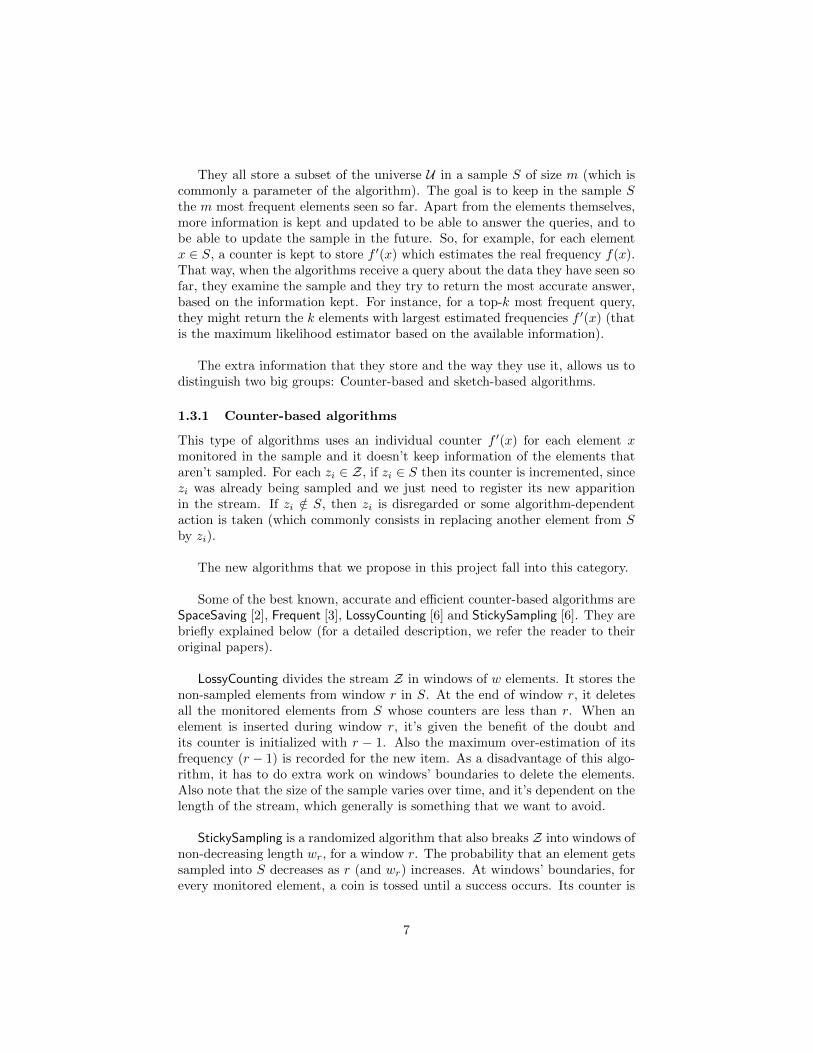
1.3.1 Counter-based algorithms
This type of algorithms uses an individual counter f ′(x) for each element xmonitored in the sample and it doesn’t keep information of the elements thataren’t sampled. For each zi ∈ Z, if zi ∈ S then its counter is incremented, sincezi was already being sampled and we just need to register its new apparitionin the stream. If zi /∈ S, then zi is disregarded or some algorithm-dependentaction is taken (which commonly consists in replacing another element from Sby zi).
The new algorithms that we propose in this project fall into this category.
Some of the best known, accurate and efficient counter-based algorithms areSpaceSaving [2], Frequent [3], LossyCounting [6] and StickySampling [6]. They arebriefly explained below (for a detailed description, we refer the reader to theiroriginal papers).
LossyCounting divides the stream Z in windows of w elements. It stores thenon-sampled elements from window r in S. At the end of window r, it deletesall the monitored elements from S whose counters are less than r. When anelement is inserted during window r, it’s given the benefit of the doubt andits counter is initialized with r − 1. Also the maximum over-estimation of itsfrequency (r − 1) is recorded for the new item. As a disadvantage of this algo-rithm, it has to do extra work on windows’ boundaries to delete the elements.Also note that the size of the sample varies over time, and it’s dependent on thelength of the stream, which generally is something that we want to avoid.
StickySampling is a randomized algorithm that also breaks Z into windows ofnon-decreasing length wr, for a window r. The probability that an element getssampled into S decreases as r (and wr) increases. At windows’ boundaries, forevery monitored element, a coin is tossed until a success occurs. Its counter is
7

decremented for every unsuccessful toss, and the element is deleted if it reaches0. It also implies extra work on windows’ boundaries and a non-fixed-size sam-ple S.
Frequent extends early work done in [7]. When |S| < m, S is filled by thenext distinct elements that appear in the stream, initializing their counters to1. When |S| = m and an element x ∈ S appears in the stream, its counter isincremented. If x /∈ S then the counters of all the elements in s are decreasedby one. When a counter reaches 0, the counter’s element is removed from S andthe next element x /∈ S that appears in Z will take its spot and be inserted intoS.
SpaceSaving is one of the most popular algorithm (to our knowledge) sinceit is intuitive, it is very efficient and reasonably simple to implement. It alsooffers tight and improved error bounds and interesting theoretical guarantees.It keeps a sorted data structure for the sample S, in which the elements areordered by the values of their counters. When an element x ∈ S appears inthe stream, its counter is updated. If it wasn’t in S, the sampled element withlower counter is replaced by x. And x inherits the replaced element’s counter(stealing its estimated frequency) and it’s incremented by one. Later, we willanalyze deeper this algorithm since some of our new ones are based on it. Butbasically, it’s important to note that it has constant time cost to process a newelement thanks to how the data structure for S is chosen. Also it can answerthe queries efficiently since the data structure is already sorted.
1.3.2 Sketch-based algorithms
This type of algorithms doesn’t monitor a subset S ⊂ U . Instead, they monitorall the elements in U in a clever way, using a family F of random hash functions.They work in a similar way as a Bloom Filter works. They have a set of counterswhich are shared by all the elements from U (like the entire bitmap is sharedin a Bloom Filter).
Basically, for each zi, a subset of |F | counters is chosen using the hash func-tions from F . Then, those counters are modified. The frequency of an elementcan be queried by observing the values of its “representative” counters and giv-ing a value depending on them. However, some loss of accuracy is expected dueto hashing collisions.
CountSketch [4] finds the representative counters of an element and incre-ments some of them while decreasing the others. The estimated frequency of anelement will be the median of its representative counters. To be able to answerthe queries for the problems that we deal with in this thesis (Heavy Hittersand Top-k), it’s necessary to keep a heap with the m elements with highestestimated frequency, which will be the sample S.
8
CountMin [5] is a modification of CountSketch. The only difference is thatall the representative counters are incremented, and the estimated frequencyof an element is the minimum value of its representative counters. This way,the estimated frequency will be an upper bound of the real frequency of thatelement, since that counter has been incremented in each apparition of it (plussome more times due to collisions of other elements).
2 Metrics
In order to evaluate and compare the performance of the algorithms with thedifferent streams, we define and use some metrics.
The metrics will measure efficiency and accuracy. For the efficiency, theused metrics are the traditional measures such as running time and memoryconsumption. To evaluate the accuracy/quality of the algorithms we will useconventional metrics, namely, recall and precision, often used in the literature.But in our view these two metrics fail short to capture the main relevant featuresof the problem and to discriminate well among the different algorithms, and thuswe have introduced a new metric which we discuss in this section in detail.
2.1 Recall and precision
As we have mentioned, we will use the standard definitions of recall and pre-cision from information theory. These two metrics where developed and areextensively used in the area of Information Retrieval, including in the existingliterature for the Heavy Hitters and Top-k problems. The formal definition isdetailed bellow.
Let A be the set of heavy hitters, and let B be the set of elements returnedby the algorithm when answering a query. Let rank(x) be the position of x inS sorting by f ′(x).
Hence, for the Top-k problem:
A = {xj ∈ U|1 ≤ j ≤ k} B = {xj ∈ S|rank(xj) ≤ k}
And for the Heavy Hitters problem:
A = {xj ∈ U|f(xj) ≥ φ} B = {xj ∈ S|f ′(xj) ≥ φ}
Then, we define recall as:
R =
∑x∈A∩B 1∑x∈A 1
=|A ∩B||A|
And precision as:
P =
∑x∈A∩B 1∑x∈B 1
=|A ∩B||B|
9
Note that 0 ≤ R ≤ 1 and 0 ≤ P ≤ 1. Also note that R = 1 ⇐⇒ A ⊆ B,meaning that the recall is maximum iff all the heavy hitters are returned by thealgorithm. R = 0 iff no heavy hitter is returned. And similarly for the precision,P = 1 ⇐⇒ B ⊆ A meaning that all the elements returned are heavy hitters,and P = 0 iff none of the returned elements is a heavy hitter (assuming thatB 6= ∅).
An intuitive understanding of the recall is that it’s a metric that requiresthe algorithms to return as many heavy hitters as possible. And the precisionrequires that the returned elements are as “pure” as possible since it measuresthe proportion of heavy hitters among the returned elements. So an algorithmthat returns all the heavy hitters by returning a huge set of elements, it willhave a high recall but low precision. And vice versa, if the algorithm returns asmall set of heavy hitters but only heavy hitters, the precision will be high butthe recall will be low. So the goal of an algorithm is to return exactly the heavyhitters, that is to be as close as possible to the “ideal” R = P = 1.
On the other hand, notice that R = 0 if and only if P = 0.
Last but not least, in the case of the Top-k problem (which is the one inwhich we have focused our efforts), we have |A| = |B| = k, that is, for the Top-kproblem recall and precision are identical (R = P ).
2.2 Weighted recall
We propose a generalization of the recall that we call weighted recall, or Rw.To our knowledge, this metric is new and we haven’t seen it in the existingliterature.
The idea is to have a metric that penalizes more to miss an element xa thanan element xb with a < b. So we weight the “importance” of an element x byusing its relative frequency p(x). Hence:
Rw =
∑x∈A∩B p(x)∑x∈A p(x)
Note how we also have that 0 ≤ Rw ≤ 1.
We believe that this metric is very useful since in most of the use cases, theharmful effect of missing the top-1 heavy hitter is much bigger than the effectof missing the kth heavy hitter.
However, we can’t use a similar generalization of the precision, since thestraightforward definition of Pw would reward an algorithm that retrieves less
10

frequent elements. The definition of weighted precision would be:
Pw =
∑x∈A∩B p(x)∑x∈B p(x)
And a situation in which Pw rewards an algorithm that returns worse elementswould be, for example, the following: Consider B and B′ such that A ∩ B =A∩B′ and |B| = |B′|. If ∀x∈B∀x′∈B′f(x) ≥ f(x′), then Pw(B) ≤ Pw(B′). Thishappens because the two expressions share the numerator, and the one withlower denominator (B′) would obtain a higher precision. But if B′ has a lowerdenominator, then B′ contains less frequent elements than B.
Hence, for the Top-k problem we will use the precision (which is the sameas the recall) and the weighted recall during the experiments.
2.3 Squared error
We will also use the well known squared error of the estimated frequencies. Moreformally:
E =∑x∈U
(f(x)− f ′(x))2,
where by convention, we take f ′(x) = 0 if x /∈ B.
E ≥ 0 will be minimum when A = B and f ′(x) = f(x) for x ∈ B.
3 The algorithms
The main algorithm that we propose in this thesis is called LotterySampling.However, we will describe other simpler versions first, constructing LotterySam-pling iteratively.
This thesis has had a big component of exploration and most of the effortshave been applied to discover the algorithms and to experiment and improvethem iteratevely. However, the depth of the theoretical analysis is limited, sincewe considered it out of scope. We will focus on giving the intuitions of why theywork well and the ideas on which they are based. We will leave for future worka more in-depth analysis and formal proofs. For example, the ultimate goalwould be to include LotterySampling into the δ-ε-deficient framework in whichother state-of-the-art algorithms are in.
3.1 BasicLotterySampling
All of our algorithms are based on the idea of what we call lottery tickets andlottery tokens. A lottery token (or token) is an independent uniform randomnumber between 0 and 1. Basically, we will generate one of such tokens for each
11
item zi that appears on the stream. And each element xj will have its ownlottery ticket (or ticket), which will be the highest token obtained among all itsapparitions so far.
In BasicLotterySampling we will have a sample S of fixed size m. And theelements that will be in this sample are the ones with highest lottery ticket. Thereason behind using the word “lottery” is that we can define an analogy witha regular lottery: In a regular lottery, there are some winners between the par-ticipants, and they are randomly chosen by selecting a subset of lottery tickets.The more lottery tickets a participant has, the more chances it will have of win-ning. And similarly in BasicLotterySampling, the more frequent an element is,the more lottery tokens it will get, so it will have more chances of getting a highlottery ticket. If its lottery ticket is among the m-highest lottery tickets, it willstay in the sample, or following the analogy, be one of the winners of the lottery.
We can formalize more the previous explanation:
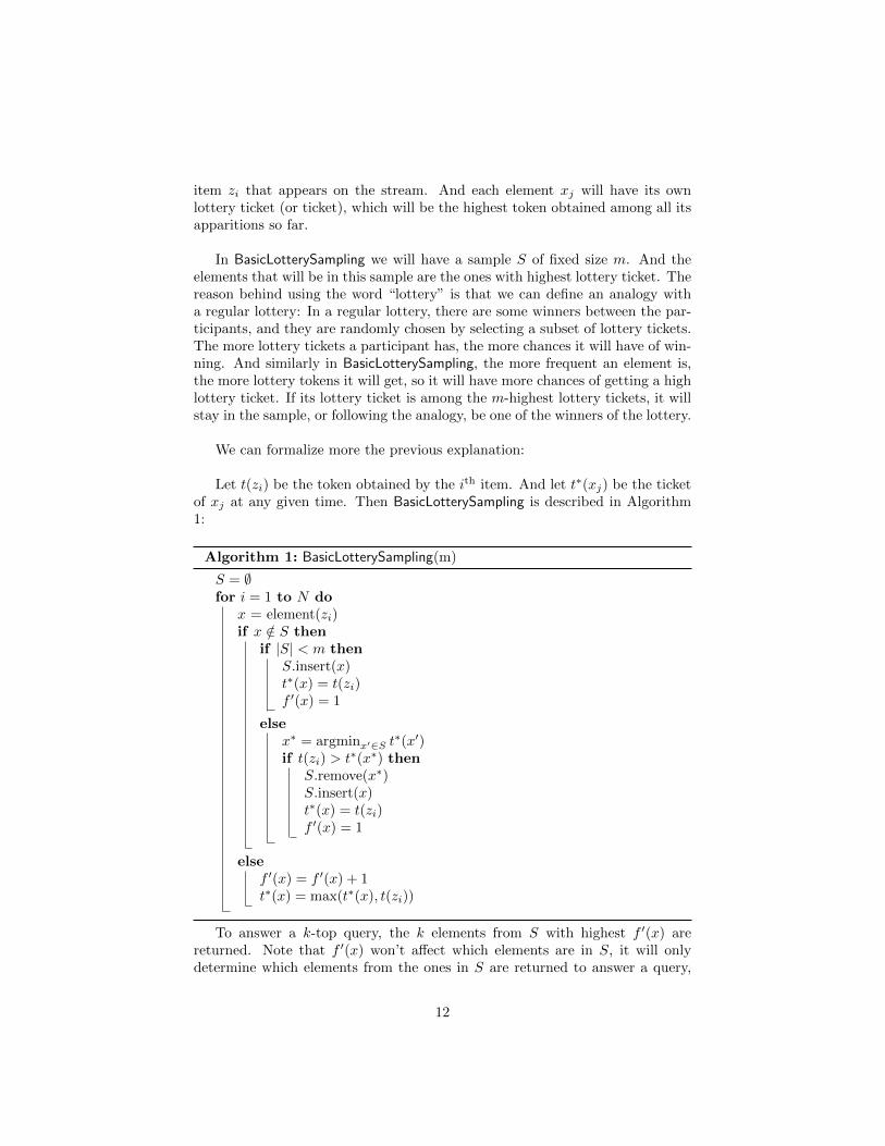
Let t(zi) be the token obtained by the ith item. And let t∗(xj) be the ticketof xj at any given time. Then BasicLotterySampling is described in Algorithm1:
Algorithm 1: BasicLotterySampling(m)
S = ∅for i = 1 to N do
x = element(zi)if x /∈ S then
if |S| < m thenS.insert(x)t∗(x) = t(zi)f ′(x) = 1
elsex∗ = argminx′∈S t
∗(x′)if t(zi) > t∗(x∗) then
S.remove(x∗)S.insert(x)t∗(x) = t(zi)f ′(x) = 1
elsef ′(x) = f ′(x) + 1t∗(x) = max(t∗(x), t(zi))
To answer a k-top query, the k elements from S with highest f ′(x) arereturned. Note that f ′(x) won’t affect which elements are in S, it will onlydetermine which elements from the ones in S are returned to answer a query,
12
and in which order.
Note that we initialize f ′(x) = 1 when we insert a new element x in thesample while replacing another. However there are other alternatives. Letfobs(x) be the observed frequency of x (i.e., the count of apparitions of x fromwhen it entered into S), and let finit(x) be the initial frequency that we estimatewhen x enters into the sample. Then, f ′(x) = finit(x) + fobs(x). In Algorithm1 we used finit = 0, so f(x) ≥ f ′(x) = fobs(x). However, we propose two otherestimations of the initial frequency:
• finit(xj) = E[f(xj)|T (j) = t∗(xj)] =⌊
t∗(xj)1−t∗(xj)
⌋. That is, we estimate the
initial frequency of xj by calculating the frequency it needed to get itslottery ticket if Var[T (j)] were 0. The definition of the random variableT (j) is detailed in the next chapter.
• finit(x) =⌊
11−t∗(x∗)
⌋. The probability for xj to enter the sample in this
apparition was 1− t∗(x∗). And the idea is to assume that this probabilityhas always been the same, so we can model it with a geometric distribu-tion. So this is an upper bound of the expectation of the number of timesx needed to appear until it entered into the sample.
The estimation that seems to work better in our experiments is finit(x) = 0.Hence, we will use this estimation in the experiments.
3.1.1 Analysis
Let t = t∗(x∗). We can view t as a “threshold”, since it’s the value that theitems need to beat with their tokens to enter the sample. Note that the thresh-old never decreases and it always increases after an insertion (when |S| = m).
Let T(j)r = t(zi) such that zi is the rth apparition of xj in the stream Z. Or
equivalently, the token obtained by element xj on its rth apparition. Observe
that T(j)r are independent uniformly distributed random variables between 0
and 1. Hence:Pr[T (j)r ≤ y
]= y
Let T (j) = t∗(xj). T(j) is also a random variable and can be expressed in terms
of T(j)r as follows:
T (j) = max(T
(j)1 , T
(j)2 , . . . , T
(j)f(xj)
)
13
The probability distribution of T (j) is:
Pr[T (j) ≤ y
]= Pr
[T
(j)1 ≤ y ∧ T (j)
2 ≤ y ∧ . . . ∧ T (j)f(xj)
≤ y]
=
f(xj)∏r=1
Pr[T (j)r ≤ y
]= yf(xj),
which is the cumulative distribution function (CDF). Taking derivatives withrespect to y, we obtain the probability density function (PDF) of T (j):
f(xj) · yf(xj)−1
The expectation of T (j) is then:
E[T (j)
]=
∫ 1
0
y · f(xj) · yf(xj)−1dy
=
∫ 1
0
f(xj) · yf(xj)dy
=f(xj)
f(xj) + 1
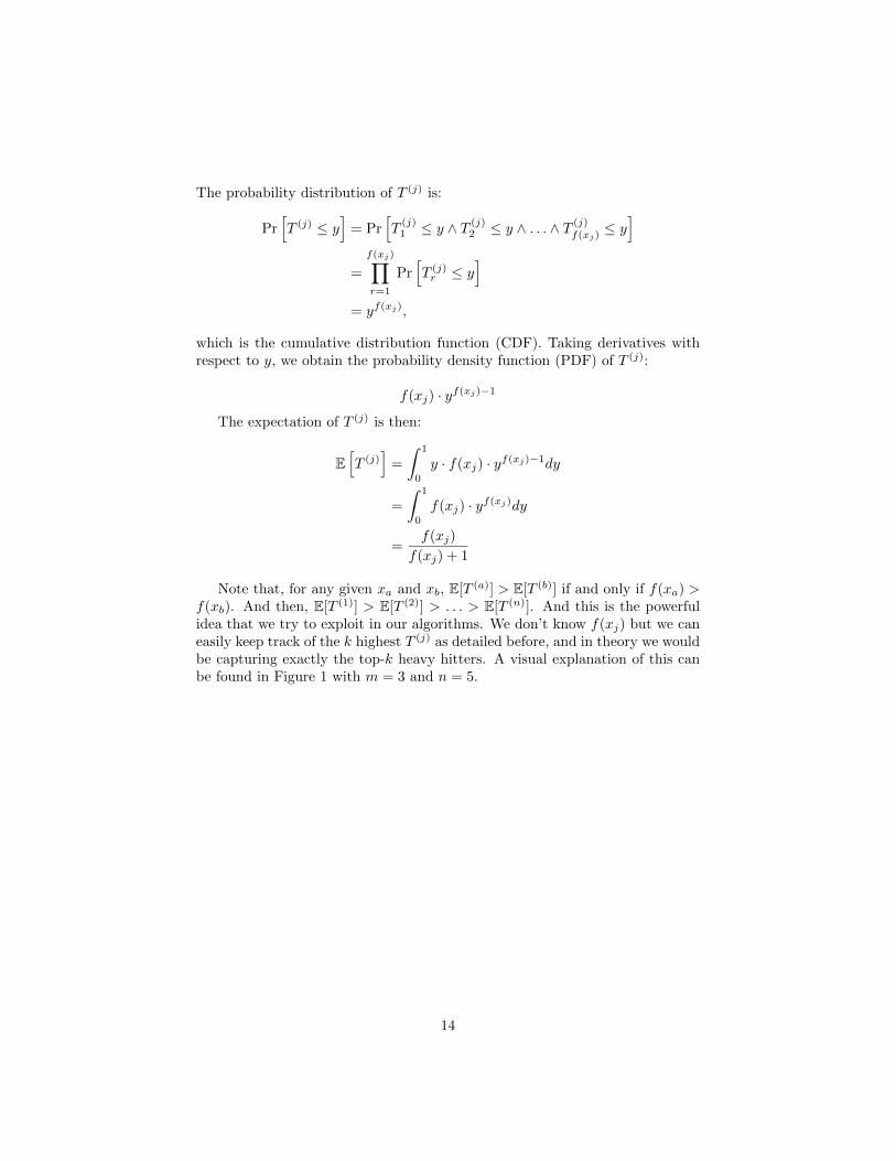
Note that, for any given xa and xb, E[T (a)] > E[T (b)] if and only if f(xa) >f(xb). And then, E[T (1)] > E[T (2)] > . . . > E[T (n)]. And this is the powerfulidea that we try to exploit in our algorithms. We don’t know f(xj) but we caneasily keep track of the k highest T (j) as detailed before, and in theory we wouldbe capturing exactly the top-k heavy hitters. A visual explanation of this canbe found in Figure 1 with m = 3 and n = 5.
14

Figure 1: Illustration of BasicLotterySampling
So if T (j) = E[T (j)] then we could solve the problem exactly. Obviously thisis not the case. Because of the variance Var[T (j)], the random variables T (j)
won’t always have the value of their expectation. i.e., One element may obtaina higher (or lower) ticket than the one it “deserves” according to its frequency.This may result in keeping in S a less frequent element instead of another withhigher frequency. For example, in the example from Figure 1, if t∗(x4) > t∗(x3),then x4 will be wrongly kept in the sample instead of x3. In fact, the probability
of this happening is f(x4)f(x3)+f(x4)
, because:
Pr[T (a) > T (b)
]= 1− Pr
[T (a) ≤ T (b)
]= 1−
∫ 1
0
Pr[T (a) ≤ y|T (b) = y
]· Pr
[T (b) = y
]dy
= 1−∫ 1
0
yf(xa) · f(xb) · yf(xb)−1dy
=f(xa)
f(xa) + f(xb)
The rest of the algorithms that we present in this work try to decrease the
15
harmful effect of the variance.
There is also another challenge that all of our algorithms will face. Notethat:
limN→∞
E[T (j)] = 1 limN→∞
Var[T (j)] = 0
This is due to the fact that while maintaining the distribution of the streamZ, the theoretical relative frequencies p(xj) will stay the same, but the absolutefrequencies f(xj) = p(xj) · N will increase, having more tokens, which makesthe expectation tend to 1 and the variance tend to 0. So although we can ex-pect lottery tickets nearer to their expectation, their values will be very closebetween them and, although the variance will be small, a very little variancewill affect enormously which elements will be kept in the sample.
A different way to illustrate the problem of the variance is the following:There are k heavy hitters in the stream and n− k non-heavy hitters. The sumof frequencies of the non-heavy hitters is Q = N − (f(x1)+f(x2)+ . . .+f(xk)).Consider k groups of the non-heavy hitters such that the sum of apparitionsof the elements in each group is approximately W ≈ Q
k . In difficult streams(where the skewness is not very big), W � f(x1), and specially W � f(xk).This means that each of the k groups will collect W tokens among its mem-bers and we expect at least one non-heavy hitter on each group to get a token(and thus a ticket) higher than the ticket of some heavy hitter(s). This willresult in replacing the heavy hitters by non-heavy hitters in S. We name thisphenomenon “element alliance”, since a way to interpret it is that non-heavyhitters will combine their tokens to obtain very high tickets such that one ofthem will enter S.
BasicLotterySampling doesn’t work well because of these reasons, as shownlater in the experiments.
3.1.2 Asymptotic cost
The memory cost of BasicLotterySampling is O(m) since we just keep a counterand a ticket for every element in the sample, whose size is upper bounded bym.
The time cost per each item is O(log(m)) since we have to store S in a minheap in order to retrieve the element with minimum ticket fast. Note that foreach apparition zi of the element xj /∈ S, we will only insert it with probability1− t, where t is the threshold. As we process the stream, the current thresholdnever decreases—it actually increases whenever an element enters the sampleand it might increase whenever we process an element already in the sample—and hence, more and more items will be ignored. Processing each of these itemshas cost O(1).
16

Note that if we want to answer queries efficiently, we should also sort Sby f ′(x) to answer the top-k queries in O(k) time, which doesn’t increase theasymptotic cost. Finally, note that we need a hash map to efficiently decidemembership of S and to locate the elements in S.
3.2 ParallelLotterySampling
One approach that we propose to solve the problem of the variance that Basi-cLotterySampling has is to independently run H parallel instances of BasicLot-terySampling with different random seeds. The idea is to combine the queryanswers of the H instances into one, decreasing the harmful effect of the vari-ance. We call this algorithm ParallelLotterySampling.
Before detailing ParallelLotterySampling, the motivation is shown empiricallythrough different experiments in figure 2. What we aim to show is that thevariance of the average of H tickets (H maximum tokens from H differentexecutions) decreases when we increase H. The Subfigure 2a shows the evolutionof the lottery ticket T (j) for a given element xj through a stream in a singleexecution. And we also plot the expected lottery ticket for each frequency. Sofor every apparition of xj (x axis), T (j) and E[T (j)] (y axis) are updated. InSubfigure 2b we also plot T (j) but for 10 different executions. In Subfigure 2c weplot the evolution of the average of the T (j)s from the 10 different executions.And in Figure 2d we plot the same but for 100 executions.
17

(a) Evolution of ticket from one execution (b) Evolution of tickets from 10 executions
(c) Evolution of mean ticket from 10 executions (d) Evolution of mean ticket from 100 executions
Figure 2
The problem that BasicLotterySampling had was the variance of T (j). Andas shown in Figure 2, by applying the average of H tickets from H indepen-dent executions, the averaged ticket is much closer to the expectation. In fact,let T ′(j) be the averaged ticket of xj from H independent executions. Then
Var[T ′(j)] = Var[T (j)]H .
18
At first glance this seems to solve the problem with a big enough H. How-ever, this implies knowing the H tickets of each distinct element. i.e, An elementmight not have a top-m ticket in all the H executions, and we still need thosetickets to do the average.
So instead of trying to decrease the variance of T (j), we will try to decreasethe variance of BasicLotterySampling by executing it H times and by combiningthe results afterwards. So the intuition is: If an element is one of the heavyhitters, then we expect it to get a large enough ticket in some of the H instancesto get inside the corresponding samples. Then we use some strategy to unifythe results from the H instances.
More formally, ParallelLotterySampling runs H instances of BasicLotterySam-pling. That means that for each item zi, it will generate H tokens and updatethe samples Sh (where 1 ≤ h ≤ H) independently following the description inAlgorithm 1. Let S be the union of all the Sh. We can view S as a sample thatcontains the elements that obtained a high ticket in some of the Sh samples.We may consider ParallelLotterySampling as a Monte Carlo algorithm: the prob-ability for a given heavy hitter to appear in S will increase with the number ofinstances. The heavy hitters will have more preference to appear in the answerof a query thanks to the strategy that unifies the results from the H samples.
Note that (after the initial phase in which the samples Sh get filled):
m = |Sh| ≤ |S| ≤ m ·H
Also note that there will constantly be m ·H tickets, independently on the num-ber of distinct elements in S.
If we use finit(x) = 0 for each one of the H instances, then it would makesense to share the counter f ′(x) between all the instances (having |S| manycounters). This means that for each x ∈ S we only have a single counter tokeep f ′(x), instead of one counter for each sample in which x is. This singlecounter counts all the apparitions of x since it was inserted in the first sampleSh. Consider for example that a certain element x not yet sampled any sample,enters sample S3. Then it appears three more times and then, on fifth occur-rence (since it entered S3) it also enters S1. It appears two more times, butthen it’s evicted from S3. Afterwards, it appears three more times while stayingin S1. Then f ′(x) = 10 at that moment, instead of having different countersfor S1 and S3 with values 6 and 7 respectively (the counter from S3 would bedeleted when x is evicted from it). If we use another initialization finit(x) theneach instance of BasicLotterySampling that contains x in its sample may keepa separate counter f ′(x) for x, so in such a case no counter would be sharedbetween samples.
19
To answer a top-k query, ParallelLotterySampling will use a strategy to deter-mine the k most frequent elements using the information from the H samples.There is a big amount of possible strategies, and they depend on how f ′(x) isdefined. Some of them are described below:
• If we keep a single counter f ′(x) for each x that appears in at least oneof the H samples (this is possible when we have finit(x) = 0) then wepropose the following two alternatives:
– The k elements with higher f ′(x) are returned to answer a query. Itis a simple strategy and we only use the observed frequencies of theelements in S.
– For each element x in S, we compute the average of its tickets from allthe samples. If x is not inside some sample Sh then we use as ticketf ′(x)f ′(x)+1 which is a lower bound of the ticket it deserved, f(x)
f(x)+1 . The
k elements with higher averaged ticket are returned.
• If for an element x we use a different counter f ′(x) for each sample (so nocounter is shared between instances, which is not possible when finit(x) 6=0), then we propose two other alternatives:
– For each x in S, we find the maximum f ′(x) among all the sampleswhere x appears. The k elements with higher maximum estimatedfrequency are returned.
– Similar as before, but instead of the maximum we compute the av-erage of f ′(x) from the H samples (taking f ′(x) = 0 whenever xdoes not belong to the corresponding sample). The k elements withhighest average estimated frequency are returned.
The strategy that seems to work better in our experiments is the first one:using finit(x) = 0 and sharing the f ′(x) between samples, sorting by f ′(x) toanswer the queries. Hence, we will use this strategy in the comparisons againstother algorithms. The pseudo-code for ParallelLotterySampling can be found inAlgorithm 2.
20
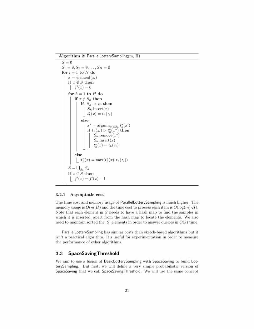
Algorithm 2: ParallelLotterySampling(m, H)
S = ∅S1 = ∅, S2 = ∅, . . . , SH = ∅for i = 1 to N do
x = element(zi)if x /∈ S then
f ′(x) = 0
for h = 1 to H doif x /∈ Sh then
if |Sh| < m thenSh.insert(x)t∗h(x) = th(zi)
elsex∗ = argminx′∈Sh
t∗h(x′)if th(zi) > t∗h(x∗) then
Sh.remove(x∗)Sh.insert(x)t∗h(x) = th(zi)
elset∗h(x) = max(t∗h(x), th(zi))
S =⋃ShSh
if x ∈ S thenf ′(x) = f ′(x) + 1
3.2.1 Asymptotic cost
The time cost and memory usage of ParallelLotterySampling is much higher. Thememory usage isO(m·H) and the time cost to process each item is O(log(m)·H).Note that each element in S needs to have a hash map to find the samples inwhich it is inserted, apart from the hash map to locate the elements. We alsoneed to maintain sorted the |S| elements in order to answer queries in O(k) time.
ParallelLotterySampling has similar costs than sketch-based algorithms but itisn’t a practical algorithm. It’s useful for experimentation in order to measurethe performance of other algorithms.
3.3 SpaceSavingThreshold
We aim to use a fusion of BasicLotterySampling with SpaceSaving to build Lot-terySampling. But first, we will define a very simple probabilistic version ofSpaceSaving that we call SpaceSavingThreshold. We will use the same concept
21

and notation from the previous algorithms of t(zi), f′(x), finit(x) and fobs(x).
In the original version of SpaceSaving, the sample S is filled by the first mdistinct elements using finit(x) = 0 and fobs(x) = 1 on their insertions. Foreach apparition of xj when xj ∈ S, we increment fobs(xj) by one. When xj /∈ Sand |S| = m, then we always insert xj by replacing the element x∗ with lowerf ′(x∗). In such cases we use finit(xj) = f ′(x∗) and fobs(xj) = 1. This can beinterpreted as xj stealing the estimated frequency of x∗. More formally:
Algorithm 3: SpaceSaving(m)
S = ∅for i = 1 to N do
x = element(zi)if x /∈ S then
if |S| < m thenS.insert(x)f ′(x) = 1
elsex∗ = argminx′∈S f
′(x′)S.remove(x∗)S.insert(x)f ′(x) = f ′(x∗) + 1
elsef ′(x) = f ′(x) + 1
To answer a top-k query, the k elements with higher f ′(x) are returned.
In order to find x∗ and to answer the queries efficiently, a data structure forS is suggested in the original paper of SpaceSaving such that updates and in-sertions are executed in O(1), with O(k) to answer the queries, which is optimal.
This data structure consists in a sorted list of buckets, where a bucket is alist of all the elements with same f ′(x). This list of buckets is sorted by f ′(x).So to replace the element x∗ with lower f ′(x∗) from S, we can access the bucketfrom one end of the list to find it. Note that f ′(x) only increases by 1 each time,so in updates and insertions of the element x, we just need to check if the nextbucket (in case it exists) contains elements with estimated frequency f ′(x) + 1.If that is the case, we just have to move x from its current bucket to the nextone. If such bucket doesn’t exist, we just have to create it next to the currentbucket and move x inside. If the previous bucket becomes empty, we delete it.All these operations can be done in O(1) time. Note that we also need a hashmap to find the elements in S.
In SpaceSavingThreshold we have a new parameter 0 ≤ t < 1 called “thresh-old”. The only modification respect to SpaceSaving is that we will only insert
22

an element x with probability 1 − t (when |S| = m). With this modification,many properties and deterministic guarantees from SpaceSaving are lost, as forexample
∑x∈S f
′(x) 6= N . However, with a properly tuned value of t depen-dent on the stream, a huge improvement can be achieved in accuracy respect toSpaceSaving. Regarding performance there is also an improvement since therewill be many less insertions (1 − t times on average), although the asymptoticcost doesn’t change.
SpaceSavingThreshold is detailed in Algorithm 4. Note that we use the sameconcept of tokens t(zi) from BasicLotterySampling:
Algorithm 4: SpaceSavingThreshold(m, t)
S = ∅for i = 1 to N do
x = element(zi)if x /∈ S then
if |S| < m thenS.insert(x)f ′(x) = 1
else if t(zi) > t thenx∗ = argminx′∈S f
′(x′)S.remove(x∗)S.insert(x)f ′(x) = f ′(x∗) + 1
elsef ′(x) = f ′(x) + 1
To understand the improvement respect to the original version it’s impor-tant to understand how the original version behaves:
When a non-sampled element x appears in the stream, SpaceSaving gives itthe benefit of the doubt and considers it a heavy hitter inserting it into S, byexpelling another element x∗. Maybe there were more elements with estimatedfrequency f ′(x∗), or maybe there was only x∗. In any case, x will inherit the es-timated frequency f ′(x∗) and increment it by one, so it will be very close to the“frontier” of S. We call frontier the bucket with smallest estimated frequency.Hence x will be dangerously near to being replaced by another element fromthe stream. If x receives more hits soon (there are more apparitions of x), itmay be able to move away from the frontier (that is, its counter f ′(x) becomessignificantly larger than the minimum counter f ′(x∗) that defines the frontier).If x is actually a heavy hitter, this separation will be easier since it will receivemore hits than the non-heavy hitters. Hence, we can intuitively visualize this asa race between the elements trying to “survive” in S, where every time an ele-ment enters into S, it starts next to the frontier. The more frequent an elementis, the faster it will run away from the frontier. At the same time, the frontier
23

will move forward every time all the elements in the frontier are replaced orreceive a hit.
If there is not much skewness in the stream (i.e., many heavy hitters havefrequencies not that different from many non-heavy hitters) most of the ele-ments in S will be very near to the frontier, being replaced constantly withouthaving enough time to run away from it. However, if the heavy hitters have ahigh enough frequency we will find the heavy hitters sorted by f(x) in bucketsfar away from the frontier. In the frontier there will be some elements (at leastone) that are constantly being replaced. In that case, the sum of frequencies Qof the non-heavy hitters is not high enough for the frontier to move faster andto reach the heavy hitters that have separated from it.
Let 1 ≤ V ≤ m be the number of elements in the frontier, then the frontierwill move to the next estimated frequency once every V new insertions (roughly,since the frontier can also move if all the elements in the frontier receive a hit).This means that an element x needs to have a relative frequency p(x) > 1
V inorder to separate from the frontier (necessary but not sufficient). Then, if Sis full of non-heavy hitters (most of them in the frontier), a heavy hitter willhave more time to get away from the frontier since the frontier will move slower.However, note that as more heavy hitters get away from the frontier, the frontierwill become smaller in size (with less elements), which will increase its “speed” 1.
By introducing the threshold in SpaceSavingThreshold we decrease the speedof the frontier, since less elements will be inserted. Hence, the heavy hitterswill have much more time to get away from the frontier, which actually meansthat they can have a much smaller frequency and still be sampled. So in dif-ficult streams where the skewness is low (and the heavy hitters have a smallfrequency), a properly tuned value of t will allow us to keep the heavy hittersin S. In fact, an element x needs to have a relative frequency p(x) > 1−t
V inorder to separate from the frontier (necessary but not sufficient). Note thatwith values of t close to 1 this requirement is much lower (and better) than inthe original version of SpaceSaving, in which p(x) needs to be greater than 1/m.So we are interested in choosing a high value of t.
However, if we choose a value for t that is too high, then the heavy hittersmay not be able to even enter the sample. Hence, we are also interested in hav-ing a low enough value of t that guarantees that the heavy hitters will pass the
threshold at some point. So for a heavy hitter x we want to have f(x) >⌈
11−t
⌉.
The optimal value of t is difficult to define, and it depends on the stream,including the distribution it follows and its length. This makes SpaceSavingTh-
1We can formally define the speed of the frontier in the interval [i, i+D] taking the differencebetween the minimum frequency in the sample when inspecting zi and the minimum frequencyin the sample when inspecting zi+D, and dividing by D.
24

reshold much less interesting, since it needs tuning and/or previous knowledgeof the stream.
3.3.1 Asymptotic cost
As mentioned before, the time cost of SpaceSavingThreshold (and SpaceSaving)is O(1) for both insertions and updates. To answer a top-k query it needs O(k).
The memory cost is O(1). The number of buckets will always be between 1and m. The union of elements from all the buckets will be all the elements inS.
3.4 LotterySampling
LotterySampling is the main algorithm that we propose in this thesis. It’s basedon the intuitions explained in the previous algorithms and it’s very accurate,substantially outperforming existing algorithms.
It’s basically a fusion of SpaceSavingThreshold and BasicLotterySampling. Ituses the ideas behind BasicLotterySampling to dynamically choose the value t ofSpaceSavingThreshold. It’s detailed in Algorithm 5.
Algorithm 5: LotterySampling(m)
S = ∅for i = 1 to N do
x = element(zi)if x /∈ S then
if |S| < m thenS.insert(x)f ′(x) = 1t∗(x) = t(zi)
elset = minx′∈S t
∗(x′)if t(zi) > t then
x∗ = argminx′∈S f′(x′)
S.remove(x∗)S.insert(x)f ′(x) = f ′(x∗) + 1t∗(x) = t(zi)
elsef ′(x) = f ′(x) + 1t∗(x) = max(t∗(x), t(zi))
If x is not in S, we insert it only if its token is higher than the minimumticket in the sample. However, instead of replacing the element with the min-
25
imum ticket (as it’s done in BasicLotterySampling), we replace the element x∗
with lowest estimated frequency f ′(x∗) (in case of tie, any is chosen). For thatreason what we call ticket in LotterySampling is not exactly a ticket in the sensegiven in BasicLotterySampling. Because an element xj could have obtained itsmaximum token (its ticket) and be in S, be expelled because it had the lowestf ′(xj) at some point and be inserted again with a lower token, so its true ticketgets lost. Hence, in the context of LotterySampling, an element’s ticket is itshighest token obtained since its last insertion into S. We will use “real ticket”to refer to the original definition of ticket.
Note how in LotterySampling, the threshold t never decreases, but it doesn’talways increase in insertions (as opposed to BasicLotterySampling, that alwaysincreases in insertions). In fact, the threshold only increases if the replaced ele-ment from an insertion was the element with minimum ticket, or if the elementwith minimum ticket receives a hit that increments its ticket. Also note thatwith the same stream and with the same sequence of tokens, the threshold inLotterySampling will always be equal or lower than the threshold in BasicLot-terySampling.
LotterySampling basically follows the idea of BasicLotterySampling, becauseit intends to keep in S the elements with highest real tickets, but it doesn’t relaycompletely in the tickets. So if a non-heavy hitter gets very lucky and obtains avery high ticket when entering into S, it won’t mean it will stay in the sampleindefinitely, because if it doesn’t get enough hits soon it will be expelled fromS, since it won’t be able to get away from the frontier faster than the real heavyhitters that are in S.
Hence, for an element to be in S, it needs to obtain a high ticket to enter Sand to have a high frequency relative to the rest of the elements to avoid beingexpelled from it.
LotterySampling has the good property from SpaceSavingThreshold that al-lows the heavy hitters to have a small relative frequency and still be kept in S.Since the threshold t can only increase, the heavy hitters will have increasinglymore time to move away from the frontier.
Also, since the non-heavy hitters are not going to survive in S, t will be someheavy hitter’s ticket most of the time. That means that t won’t increase too fastbecause the “element alliance” phenomenon suffered by BasicLotterySamplingwon’t affect it that much. So t will have a similar value to the expected realticket from some heavy hitter xj with j near to k. Then j out of the k heavyhitters should be able to overpass the threshold (since their expected real ticketis higher), solving the problem of SpaceSavingThreshold when choosing a fixedand (possibly too) high t.
26
3.4.1 Asymptotic cost
The asymptotic cost per item of LotterySampling is the same as in BasicLot-terySampling, since we need to find the lowest ticket in S by using a heap.LotterySampling can use the efficient data structure from SpaceSaving to keepthe elements sorted by f ′(x) with cost O(1), although it will be dominated bythe cost of the heap.
Then the time cost of LotterySampling is O(log(m)) and it has a memoryusage of O(m). To answer a top-k query it will take O(k) by using the Space-Saving’s data structure.
3.5 Other variations
In the exploratory phase of this thesis we considered some ideas to improvethe algorithms or to solve some of their problems. However, we haven’t fullyexperimented with them so they are not merged in the proposed version ofLotterySampling nor are they included in the experiments of this document. Wesummarize some of these ideas in the following subsections.
3.5.1 LotterySampling with ticket scaling
One implementation problem that LotterySampling has is the resolution of thetokens and tickets. The threshold will approach arbitrarily to 1 with arbitrarylong streams, so the precision of the binary representation will affect the algo-rithm. Consider a natural number v ∈ [0, 2b) using b bits to represent a tickett∗(x), such that t∗(x) = v/2b.
One possible solution that we call “ticket scaling” consists in scaling thetickets when the threshold overpasses the value 1− 2−r for any r. Note that insuch cases, the threshold will contain r leading ones in its binary representationv. Since the threshold never decreases and all the other tickets in S need tobe equal or higher, then all the current tickets in S will also have r leadingones in their binary representations. So we can always remove as many leadingones that the threshold has from all the tickets in S, and keep track of thenumber of removed leading ones so far. The removal of the ones is done byshifting the binary representation of the tickets to the left and adding zeros tothe right. This way, we regain precision by not wasting bits that will alwayscontain ones. The generation of the next tokens needs to be slightly adaptedto this modification. For example, first a random number is generated to makesure that the new token also has r leading ones, and then we generate the restof the ticket.
3.5.2 BasicLotterySampling with ticket aging
It is possible to add a degradation or decay with time to the tickets in S, mean-ing that the tickets will loose value while they get older. Hence, in this variation
27

the tickets in S will decrease over time following some criteria. This decay couldbe exponential or linear. The idea is to force the elements to keep getting hightokens, so it wouldn’t be enough to get a large one once to stay in the sample.
The problem it has is that it’s difficult to choose an aging function for thetickets, and that this function probably needs some extra parameters. We havetested some approaches with both linear and exponential aging and it allowsthe algorithms to improve substantially but requiring stream-dependent tuning.This idea can also be applied to LotterySampling.
3.5.3 LotterySampling adapted for the weighted setups
As mentioned previously, there exists a weighted version of the Heavy Hittersand Top-k problems in which each item zi has some weight wi ∈ N, and for theelement xj the frequency f(xj) is the sum of the weights from its apparitions.
We can generalize our algorithms by generating wi tokens for each appari-tion zi of the element xj , and using the highest one to update S. This wouldbe equivalent to wi consecutive apparitions of xj . Then we increment f ′(xj) bywi instead of by 1.
The problem with this approach is that the cost per item would be O(wi +log(m)). To solve it, we can compute one single token as t′(zi) = wi
√t(zi).
The random variable t′(zi) is distributed as the maximum of wi independentuniforms in (0, 1) [8]. Hence, this is equivalent to generating the wi tokens sep-arately and choosing the maximum. To see it, first note that the probabilitydistribution of the maximum of wi tokens is the same as the one from T (j),
where in this case it is Pr[t(zi) ≤ y
]= ywi .
Then, note that:
Pr[t′(zj) ≤ y
]= Pr
[wi
√t(zi) ≤ y
]= Pr
[t(zi) ≤ ywi
]= ywi
Hence both random variables have the same probability distributions. So byusing the second approach, the asymptotic time cost of LotterySampling for theweighted versions doesn’t increase.
Note that in the case of SpaceSaving, the time cost goes from O(1) toO(log(m)) since now the frequency of the elements doesn’t increase by oneand that makes its efficient data structure not suitable anymore.
3.5.4 LotterySampling adapted for the Heavy Hitters problem
In this thesis we have focused on the Top-k problem, specially when running theexperiments. The proposed algorithm for LotterySampling can also be used forthe Heavy Hitters problem, where we want to find all the elements with relative
28
frequency higher than φ.
However, we could use a simpler and more intelligent approach. We couldforget the tickets and use a threshold t exactly like in SpaceSavingThreshold,but varying the threshold through the life of the stream, such that t = φ·N
φ·N+1
(where N is the current length of the stream). In this version, t evolves exactlyas the expected ticket of an element with frequency φ. Hence, the heavy hitterswill have a higher expected ticket so we expect them to enter S.
4 Implementation
For this thesis, some of the most used algorithms for the Heavy Hitters and Top-k problems have been implemented, apart from the new ones proposed. Thegoal was to empirically compare the accuracy and efficiency of the algorithmsthrough experiments using the defined metrics, with all of them sharing thesame coding style and reusing as much as possible the underlying data struc-tures.
The implementation of the algorithms has been done in C++. A test envi-ronment to run the algorithms with different streams has been done in Python.To visualize the results both Python and Matlab scripts can be used. The entireproject can be found inhttps://github.com/GonMolon/Lottery Sampling.
4.1 Project structure
When building the project, an executable will be generated. To run it, somearguments need to be provided. These arguments will determine the used al-gorithm and its parameters, like the size of the sample S and other algorithmdependent parameters. Then, the stream is feed into the algorithm by writinginto its standard input.
Every new-line-separated string represents an ID of some element, so eachline will correspond to an item or apparition. The type of the IDs is parame-terized and both strings and numerical types are supported.
The program will instantiate the chosen algorithm and it will be called withthe corresponding ID for each item. All the algorithms need to implement aninterface called GenericAlgorithmInterface. An abstract class called Generi-cAlgorithm is offered that already implements some of the methods from theinterface, and offers some common functionalities between all the algorithms.
For example, GenericAlgorithm keeps a hash map to store and locate all thesampled elements in S. All the algorithm implementations inherit from Gener-
29

icAlgorithm and provide it the type of the sampled elements, which is a structwith all the necessary fields to keep the required information of each sampledelement. Then, GenericAlgorithm will find the instance of an element givenits ID using the hash map. If such instance doesn’t exist, then it will call theabstract method “insert element(Element)”. In case this element was alreadybeing sampled, then the abstract method “update element(Element)” is called.
The algorithm implementations basically just have to implement the twoaforementioned abstract methods. The insert element(Element) method willreturn a boolean indicating if the element needs to be kept in the sample byGenericAlgorithm. It may also remove another element if there is a replacement.
The algorithms also have to implement other methods to answer queries bywriting on their standard output.
The implemented algorithms are:
• BasicLotterySampling
• ParallelLotterySampling
• SpaceSaving
• SpaceSavingThreshold (by generalizing SpaceSaving)
• LotterySampling
• Frequent
• CountSketch
• CountMin (by generalizing CountSketch)
4.2 Implementation details
The algorithms usually need to maintain the elements with some level of order-ing. In fact, in some algorithms like LotterySampling more than one orderingis needed (order by frequency and by ticket). Hence, some data structures areneeded to maintain such orders, each one with different properties and require-ments. The list of implemented data structures is the following:
• BinaryHeap. It’s an efficient custom implementation of a binary heap overa vector, such that the ordering key of the elements can be updated. It’suseful for LotterySampling and others since the ticket of an element mayincrease while the element wasn’t at the top of the heap. The operationof replacing an element is optimized. The elements can’t be traversed inorder by their key, since that operation is not required by a heap.
30

• SortedTree. It’s a wrapper around the std::set. It’s mainly used when wewant: to traverse the elements in order by key, to insert an element withan arbitrary key, to arbitrarily modify the key of an arbitrary element andto delete an arbitrary element. It can also be used as a heap when it’srequired to traverse the elements in order. It is used by BasicLotterySam-pling to keep the elements sorted by frequency if finit(x) 6= 0. It’s alsoused by CountSketch and CountMinSketch.
• SortedList. It’s an implementation of the data structure proposed in theSpaceSaving’s paper. It consists in a list of buckets, where each bucketcontains a list of elements. It’s implemented as described in the originalpaper. It also has been described when describing SpaceSaving in thisdocument. The key of an arbitrary element can increase by 1 unit eachtime. It’s used by BasicLotterySampling when finit(x) = 0 since it’s alsopossible to remove an arbitrary element.
• SortedVector. It’s a custom and improved implementation over a vectorof the data structure proposed in SpaceSaving’s paper. Instead of havinga list of lists as suggested in the original paper, we just have a vector withall the elements sorted decreasingly by their keys. Hence, the elementswith same key will be stored contiguously. We also have a list of buckets,but in this implementation a bucket doesn’t contain a list inside. A bucketjust keeps the index of the first element from the vector that is inside thebucket, and it also keeps its key (estimated frequency in our use cases).The list of buckets is also sorted by key, and each element also keeps apointer to the bucket in which it is.
Then, when an element increments its key, we get its bucket through itspointer. Then we place the element in front of all the elements that are inthe same bucket. We do this by swapping it with the first element withthe same key that appears first in the vector. We can find this elementusing the index that the bucket maintains. We update the index of theold bucket accordingly (by increasing it by one) or delete the bucket if itbecomes empty. If the next bucket in the list of buckets already had thenew key of the element, we just need to update the pointer of the elementto point to this other bucket. If such bucket doesn’t exist, we create itnext to the old bucket in the list of buckets and we initialize its fields withthe index and the new key of the element.
This implementation is more efficient than the original implementation,both in memory footprint and execution time, since to have a vector in-stead of a list of lists is much more cache friendly and it requires lessmemory overhead. It’s used by SpaceSaving, SpaceSavingThreshold andLotterySampling.
These data structures don’t really keep the elements inside. They instead storepointers to the real elements which are located inside the hash map of Gener-
31

icAlgorithm. The struct that defines the elements needs to have fields called“locators” that are used to locate the elements inside every data structure inwhich they are. These locators are also modified by the data structures.
Also, as mentioned before, the tickets are represented with unsigned integersof 64 bits. The number of bits used affects the results because of resolution prob-lems. Some functionalities about the tickets are shared between the algorithmsso they are extracted in a TicketUtils class.
4.3 Test environment
The test environment is implemented in Python. There are experiments thatmeasure the efficiency of the algorithms (time and memory consumption) andothers that measure the accuracy.
To measure the efficiency the Valgrind profiler is used. When measuringboth the memory and the time consumed by the algorithms, the cost of theIO operations is not accounted. That is accomplished by inspecting the outputtraces of Valgrind and ignoring everything that is outside the GenericAlgorithmclass or subclasses.
Regarding the time cost that Valgrind reports: the value is not executiontime, but number of instructions executed in a virtual machine, accountingcache misses, data reads, etc.
To measure the accuracy of the algorithms, it’s necessary that the Pythonprogram keeps a counter for each element in the stream to exactly computethe heavy hitters and their exact frequencies. This is what all the proposedalgorithms intend to avoid, since it requires a lot of memory. Hence, runningexperiments that measure the accuracy of the algorithms are very time consum-ing because the computer running the tests enters into swap memory. Also, theexecutions using Valgrind are very slow due to the virtualization. Some of thetests have been performed with EC2 instances in Amazon Web Services usinghosts with more memory and more resources to address these problems.
The experiment results are saved in .csv files, and can be inspected andvisualized with Matlab. A Matlab script is also provided to that end.
5 Experimentation
5.1 Streams
To experiment with the new and existing algorithms we have used streams gen-erated from some Zipfian distribution. During the exploratory phase of theproject we have also worked with streams generated from non-Zipfian distribu-
32

tions, but the results were very similar, and the Zipfian streams show well themost relevant features of the algorithms. Moreover, there is a well established“tradition“ in the literature of using such Zipfian streams in experiments. Hence,the synthetic streams used in this documents are all Zipfian distributed streams.
We will refer to a stream that follows a Zipfian distribution with parameterα as Zipf-α-N , where N is the length of the stream. Hence, the theoreticalrelative frequency of the element xj in a Zipf-α-N stream is:
p(xj) =1/jα∑∞v=1 1/vα
,
where xj = j ∈ N and α > 1.
In particular, we will use a few values for α. The probability density functionand the cumulative probability distribution for α = 1.0001 are plotted in Figure3.
(a) PDF of Zipf-1.0001 (b) CDF of Zipf-1.0001
Figure 3: PDF and CDF of Zipf-1.0001 between x1 and x50
Note that we are only plotting the values for the top-50 heavy hitters, sincethe universe U is the entire set of naturals. Hence, the CDF doesn’t arrive to1 in its plot. Also note that for a fixed k, the frequencies of the top-k (heavyhitters) are much higher than the non-heavy hitters’. But the sum of the fre-quencies of the heavy hitters is still very low. This is why the Zipfian streams
33
are very interesting to experiment with.
We have also used a real stream from a big Internet company that we willcall RealStream. The stream consists in a sequence of requests performed to oneof the multiple clusters that are part of a distributed database. These requestswere performed during 10 minutes on a day of high traffic, and only a 10% ofthe total number of requests were sampled. This stream has N = 1.3 · 109 andits cardinality is n = 271 · 106. The full streams occupies 100 GB of storage.
5.2 Experiments
Most of the experiments that have been realized during this thesis can be dividedin three types:
1. For a single stream, some algorithms are executed once and some metricsare obtained by periodically measuring them. So in total there’s only oneexecution per algorithm sharing the same stream, and by observing theobtained results we can appreciate how the metrics evolve as the streamis processed.
2. For a single stream, some algorithms are executed multiple times by mod-ifying a common parameter between them, normally m (the size of thesample). At the end of each execution, the metrics are measured. Hence,this allows us to see how the modified parameter of the algorithms affectthe metrics at the end of the stream.
3. A fixed set of algorithms with fixed parameters are executed multipletimes, changing the stream in each execution. The metrics are measuredat the end of each execution. In these experiments, the stream is normallysynthetic and some parameter is changed. This is useful to see how theparameter of the stream affects the metrics. We will use this type ofexperiment varying the α of a Zipfian distribution.
During the exploration phase of the thesis we experimented with all theimplemented algorithms. However, in the following results we will only includea subset of the algorithms, using the ones that performed best to compare ouralgorithms against them.
Experiment 1
The first experiment consists in comparing the accuracy of BasicLotterySamplingand SpaceSaving with the stream Zipf-1.0001-107 in an experiment of type 1using top-100 queries. Both algorithms share the same parameter m = 200.Their precision and weighted recall are plotted in Figure 4.
34

(a) Precision (b) Weighted recall
Figure 4: Accuracy top-100 in Zipf-1.0001-107
Note how BasicLotterySampling doesn’t outperform SpaceSaving, having verysimilar values of precision and recall through all the stream. Also, note how theirprecision is very low, which means that they are returning just around 10% and20% of the heavy hitters.
Experiment 2
In this experiment we repeat the experiment 1 but comparing BasicLotterySam-pling, ParallelLotterySampling and LotterySampling. All three algorithms sharem = 200 and ParallelLotterySampling uses h = 10. The results are in Figure 5:
35
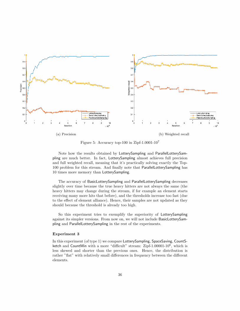
(a) Precision (b) Weighted recall
Figure 5: Accuracy top-100 in Zipf-1.0001-107
Note how the results obtained by LotterySampling and ParallelLotterySam-pling are much better. In fact, LotterySampling almost achieves full precisionand full weighted recall, meaning that it’s practically solving exactly the Top-100 problem for this stream. And finally note that ParallelLotterySampling has10 times more memory than LotterySampling.
The accuracy of BasicLotterySampling and ParallelLotterySampling decreasesslightly over time because the true heavy hitters are not always the same (theheavy hitters may change during the stream, if for example an element startsreceiving many more hits that before), and the thresholds increase too fast (dueto the effect of element alliance). Hence, their samples are not updated as theyshould because the threshold is already too high.
So this experiment tries to exemplify the superiority of LotterySamplingagainst its simpler versions. From now on, we will not include BasicLotterySam-pling and ParallelLotterySampling in the rest of the experiments.
Experiment 3
In this experiment (of type 1) we compare LotterySampling, SpaceSaving, CountS-ketch and CountMin with a more “difficult” stream: Zipf-1.00001-106, which isless skewed and shorter than the previous ones. Hence, the distribution israther ”flat” with relatively small differences in frequency between the differentelements.
36

All the algorithms share the parameter m = 100. SketchCount and CountMinalso have parameters h = 100 and q = 100 which means that they will use ah · q matrix to store the shared counters. The results are shown in Figure 6:
(a) Precision (b) Weighted recall
Figure 6: Accuracy top-100 in Zipf-1.00001-106
CountMin outperforms LotterySampling, both in precision and in weightedrecall. However, note that CountMin and CountSketch use much more memorythan LotterySampling and SpaceSaving (see Figure 8), since they keep a very bigmatrix apart from the sample S, so the comparison is not fair.
In Figure 7 we increase the length of the stream by 50, using the streamZipf-1.00001-50 · 107:
37

(a) Precision (b) Weighted recall
Figure 7: Accuracy top-100 in Zipf-1.00001-50 · 107
In this stream, which uses the same distribution as the previous one butit’s longer, LotterySampling outperforms CountMin (with much less memory).What we try to exemplify here is the need of long streams that LotterySamplinghas when their distribution is difficult. So LotterySampling works very well evenwith difficult streams, but the more difficult they are, the longer they need to be.
This behaviour is mainly related to two things:
• Var[T (j)] will be larger in difficult streams because the elements will haveless tokens, since their frequencies are smaller.
• The threshold of LotterySampling will also be smaller and it will increasemore slowly for the same reason as before: The elements have less tokensso their expected tickets will also be lower.
When the streams are longer, the elements receive more tokens solving the afore-mentioned problem.
In appendix A we show the answer of every algorithm to a top-100 query atthe end of the stream. It’s useful as a visual inspection since the k heavy hittersare 1 . . . k, so an algorithm that returns lower elements will have better accuracy.
The memory consumption of the algorithms in this experiment (with bothstreams) is shown in Figure 8:
38

Figure 8: Memory usage
Experiment 4
In this experiment (of type 3) we show how the accuracy of the algorithmsincreases when we increase the parameter α of Zipf-α-107. In all the executions,LotterySampling has m = 200, SpaceSaving has m = 1000, and CountSketch andCountMin have m = 300 and h = q = 120. This way, LotterySampling consumeshalf the memory than the other algorithms. The results are in Figure 9:
39
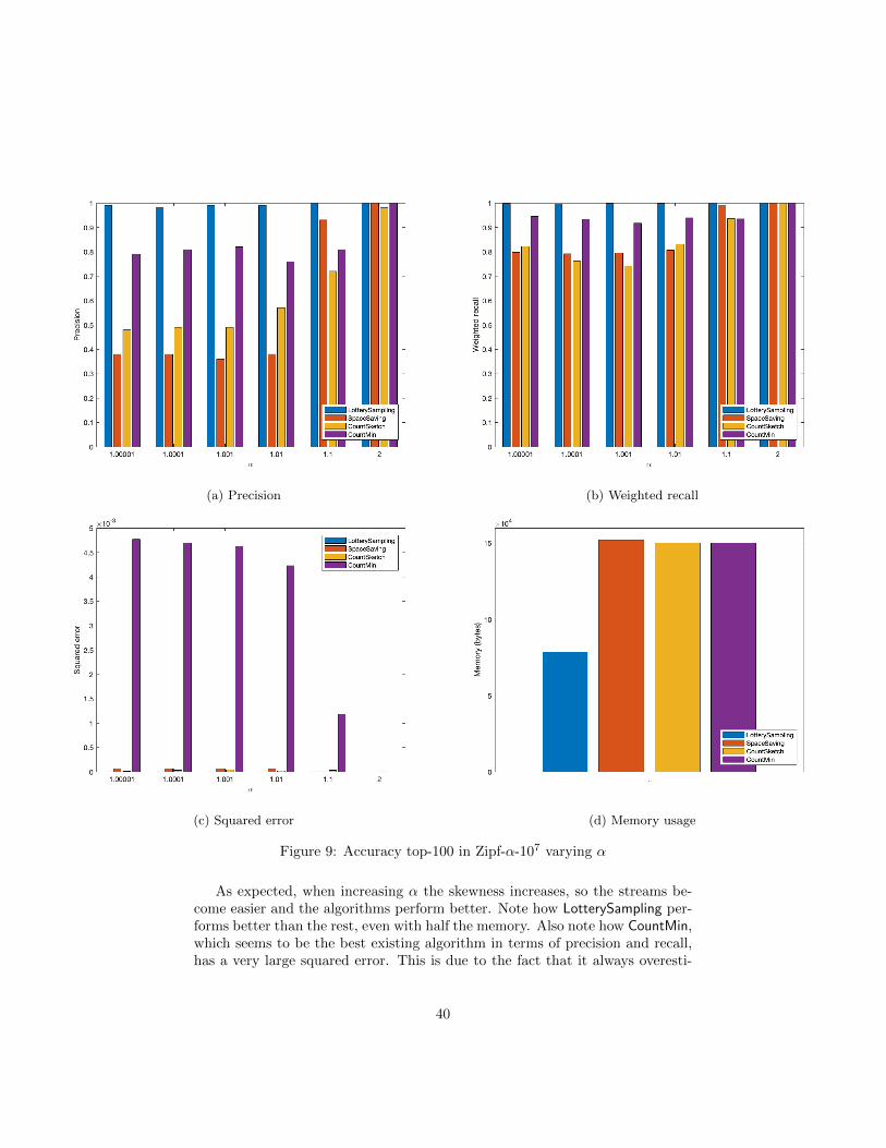
(a) Precision (b) Weighted recall
(c) Squared error (d) Memory usage
Figure 9: Accuracy top-100 in Zipf-α-107 varying α
As expected, when increasing α the skewness increases, so the streams be-come easier and the algorithms perform better. Note how LotterySampling per-forms better than the rest, even with half the memory. Also note how CountMin,which seems to be the best existing algorithm in terms of precision and recall,has a very large squared error. This is due to the fact that it always overesti-
40

mates the frequencies of the elements, and the hash collisions will increase itsestimations.
Experiment 5
In this experiment (of type 2) we aim to show how the size of the sample affectsthe accuracy of LotterySampling and SpaceSaving. Since LotterySampling almostalways achieves full accuracy with long streams, in this experiment we will usea difficult and short stream for it to be interesting.
More specifically, we use a Zipf-1.00001-106, and we will vary the parameterm from 100 to 1000, always evaluating the accuracy with a top-100 query atthe end of the stream. The results are shown in Figure 10.
(a) Precision (b) Weighted recall
Figure 10: Accuracy top-100 in Zipf-1.00001-106 varying m
This is an interesting result related with the experiment 3. LotterySamplingdoesn’t perform always better when increasing the size of the sample. This isa common behaviour of LotterySampling. The reason is that the threshold in-creases much slower when m is too big. This happens because the mth heavyhitter has a lower frequency than the kth, so its expected lottery ticket willincrease more slowly. Hence, with such a low threshold, the frontier of Lot-terySampling moves too fast and the heavy hitters don’t have time to run awayfrom it.
Then, similarly as in experiment 3, if the length of the stream is long enough
41

for a given m, the accuracy will improve again. Hence, LotterySampling needslong enough streams when the streams are very difficult or its sample is very big.In Figure 11 we execute the experiment again with the stream Zipf-1.00001-107
which is the same but 10 times longer:
(a) Precision (b) Weighted recall
Figure 11: Accuracy top-100 in Zipf-1.00001-107 varying m
Now the counter-intuitive behaviour in which LotterySampling performedworse when increasing its sample doesn’t occur anymore.
Experiment 6
In terms of efficiency, SpaceSaving is the best algorithm since it requires lowmemory (for a fixed m) and its asymptotic cost per element is O(1). CountS-ketch and CountMin are the worst in this aspect, since they require quadraticamount of memory respect to h and q, and the asymptotic cost per element isO(log(m)+h). Note that the cost per element of LotterySampling is O(log(m)).
In this experiment (of type 2) we show how the size of the sample affectsthe efficiency of LotterySampling and SpaceSaving. CountSketch and CountMinare excluded from this experiment since their efficiency is much worse. We usea Zipf-1.00001-107. The cost per item is the average. The results are plotted inFigure 12.
42
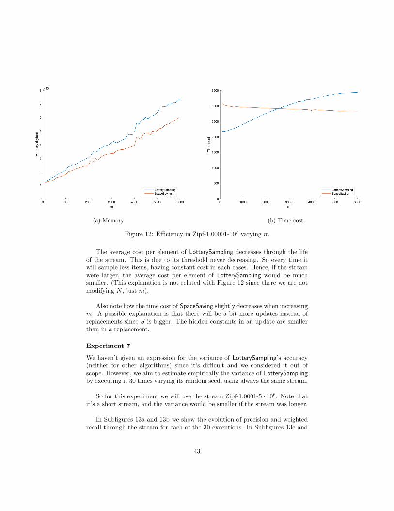
(a) Memory (b) Time cost
Figure 12: Efficiency in Zipf-1.00001-107 varying m
The average cost per element of LotterySampling decreases through the lifeof the stream. This is due to its threshold never decreasing. So every time itwill sample less items, having constant cost in such cases. Hence, if the streamwere larger, the average cost per element of LotterySampling would be muchsmaller. (This explanation is not related with Figure 12 since there we are notmodifying N , just m).
Also note how the time cost of SpaceSaving slightly decreases when increasingm. A possible explanation is that there will be a bit more updates instead ofreplacements since S is bigger. The hidden constants in an update are smallerthan in a replacement.
Experiment 7
We haven’t given an expression for the variance of LotterySampling’s accuracy(neither for other algorithms) since it’s difficult and we considered it out ofscope. However, we aim to estimate empirically the variance of LotterySamplingby executing it 30 times varying its random seed, using always the same stream.
So for this experiment we will use the stream Zipf-1.0001-5 · 106. Note thatit’s a short stream, and the variance would be smaller if the stream was longer.
In Subfigures 13a and 13b we show the evolution of precision and weightedrecall through the stream for each of the 30 executions. In Subfigures 13c and
43
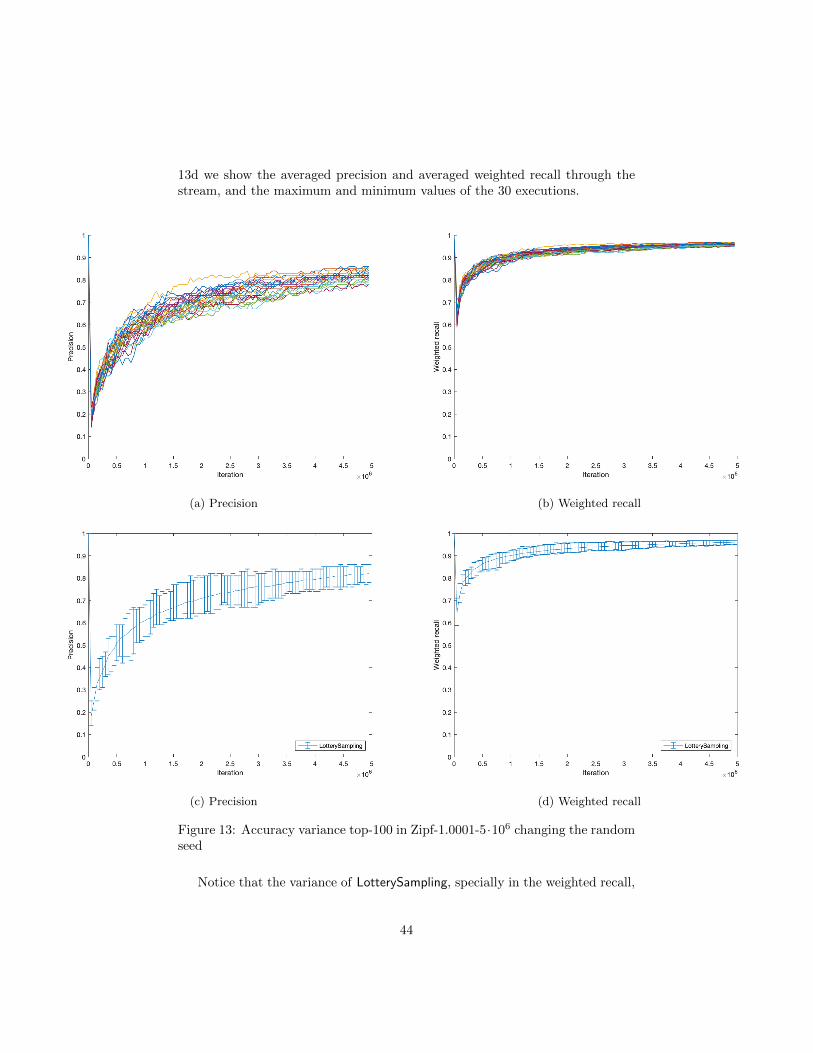
13d we show the averaged precision and averaged weighted recall through thestream, and the maximum and minimum values of the 30 executions.
(a) Precision (b) Weighted recall
(c) Precision (d) Weighted recall
Figure 13: Accuracy variance top-100 in Zipf-1.0001-5·106 changing the randomseed
Notice that the variance of LotterySampling, specially in the weighted recall,
44

is very low.
Experiment 8
This experiment is very similar to the previous one, since we want to see how thevariance of LotterySampling is when permuting the stream. Hence, we will alsouse Zipf-1.0001-5 · 106 to run 30 times LotterySampling with it, but generatinga random permutation of the stream for each execution. The results are shownin Figure 14.
(a) Precision (b) Weighted recall
Figure 14: Accuracy variance top-100 in Zipf-1.0001-5 ·106 changing the streampermutation
Note how the variance of LotterySampling is also low, very similar to theprevious experiment, indicating that LotterySampling is resistant to differentrandom permutations of the same stream. However, there exist permutationsthat harm a lot its accuracy. An example of a very harmful stream would beone with the elements appearing in decreasing order of frequency (so first allthe heavy hitters and then the rest).
Experiment 9
In this experiment (of type 1) we evaluate the accuracy of the algorithms withthe real stream called RealStream described previously. We run 2 instances ofLotterySampling with different parameter m. The results are plotted in Figure15:
45

(a) Precision (b) Weighted recall
(c) Squared error (d) Memory usage
Figure 15: Accuracy top-100 in RealStream
46
6 Conclusions
LotterySampling is a novel algorithm based upon an original and innovative idea,and the experiments and its preliminary analysis indicate that it’s far superiorto previously existing algorithm in most practical settings, including very diffi-cult streams.
We think that the given intuitions behind LotterySampling are convincing.However, much more efforts are required in giving formal proofs and theoreticalguarantees of its performance.
There are also some variations (mentioned in this document) that are promis-ing but they need to be tested and implemented more carefully, including thegeneralization for the weighted setups of the problems.
Hence, we don’t consider that this work is finished and we will try to completeit in a near future.
47

Appendices
A Visual inspection of the algorithms’ accuracy
The results of a Top-100 query at the end of a stream Zipf-1.00001-50 · 107 arethe following:
LotterySampling:1, 2, 3, 4, 5, 6, 7, 8, 9, 10, 11, 12, 13, 14, 15, 16, 17, 18, 19, 20, 21, 22, 23, 24,25, 26, 27, 28, 29, 30, 31, 32, 33, 34, 35, 36, 37, 38, 39, 40, 41, 42, 43, 44, 45, 46,47, 48, 49, 50, 51, 52, 53, 54, 55, 56, 57, 59, 58, 60, 63, 62, 61, 64, 65, 67, 66, 68,69, 71, 70, 73, 72, 74, 76, 77, 75, 78, 80, 79, 81, 84, 83, 86, 88, 91, 85, 92, 89, 93,90, 95, 96, 101, 110, 113, 103, 42471302375, 27785328369207, 630932846465970
SpaceSaving:1, 2, 406608324861036, 571345790840599872, 1792053523919, 40360142739, 112506041756,11585509175, 885300673359616, 13770390610, 11142, 1916338767215777, 3181,55481281460, 38827430309502, 648496, 432, 167783449753585376, 27775, 8074328,1125303736512322, 145072778967054, 385414796126425600, 20356216809153, 478559793,639341415366, 8650283365990666240, 1647617298061723136, 22681589409276404,502817165, 1671261867591035, 210483659248207712, 6260691795, 18572494, 19718816374,3787652552482222080, 5141148682431897600, 145947612739, 141052, 3393717,2644849072780148224, 5717047601926281216, 3505082207190, 360956028, 636907448319784960,60017807, 173276, 2660954, 461700860, 1242, 218576176488, 69, 197754970,682857, 231612, 170765644519128032, 2714, 9230081060, 1375584820474042880,781, 383844027, 5107852986673601, 2896286333170149, 17246625150675, 609587653490342,23063174403431092, 204060, 11156745, 16338021345465308, 45257539992959,17137676625147, 618026274174, 1172146731409, 1723604609, 4051204438, 146948750904,6970, 129709027657, 8, 402925541, 316690, 49, 7621992477281129, 14813078892,20560331, 798397436290895, 915103597069, 288591610041, 3024344681361, 1900634441,524718935, 588496958006234, 1464332410, 221960461174, 16646142, 1980955507102574848,677775, 5525799141262, 13947509, 719146236094
CountSketch:1, 2, 3, 4, 5, 9, 11, 12, 13, 14, 15, 16, 17, 18, 22, 25, 26, 27, 29, 30, 31, 33,34, 35, 36, 37, 38, 39, 41, 42, 44, 45, 50, 52, 56, 58, 62, 65, 126533705343901,351767713733057, 879074770758411, 16475621214935404, 151282, 2512620024,338222911753, 95124800877292, 32196446144768952, 24190367495936836, 2116798563,395590558, 1001223944578818176, 6743688163, 16165977700754436, 9580489516304,7461075738902, 1387788961621, 3256012180434895, 113852945060, 79971429004819,35046848, 2305956, 2163356075851576, 382602275355, 892515918227, 26373382431875,24988426, 376258839387, 23093621609528092, 93667146, 449922077746164608,25265721459378, 82336306, 9581664239, 80589598, 304626731569216448, 96623,656017908813, 268366119366301, 1303650026497355, 355378845045440832, 1873817819500824,1040039, 633975963982394, 19022684024718792, 215379171, 1073206969626849280,
48
1361767665, 157580046, 135287, 14663764277, 7263412729, 928481, 13636609842090848,231259172208101280, 6460698942130260, 38893398, 204998689909435, 4940165454648500224,252113176622, 2057468849156536832
CountMin:1, 6, 4, 5, 3, 12, 8, 11, 9, 15, 13, 2, 17, 26, 24, 29, 33, 28, 34, 43, 39, 21, 35, 32,7, 38, 49, 16, 30, 10, 25, 40, 66, 22, 48, 46, 19, 67, 50, 44, 84, 80, 54, 59, 42, 87,18, 56, 20, 53, 37, 71, 36, 14, 88, 90, 120, 69, 704125304292283776, 76, 61, 104,62, 47, 83, 27, 51, 105, 64, 78, 52, 112, 65, 58, 70, 94, 73, 98, 74, 136, 91, 68, 57,294066, 31, 79, 108, 23, 45, 106, 130, 55, 127, 492, 206, 41, 75, 63, 93, 155
49
B Scope and methodology
B.1 Scope
Initially, we planned to do this thesis about a new randomized algorithm in-vented by Prof. Conrado Martınez that we call BasicLotterySampling. This al-gorithm is inspired by the previous work of C. Martınez and his co-authors [1]in the related problem of cardinality estimation.
However, after the implementation of BasicLotterySampling we performedsome tests comparing its efficiency and accuracy with the popular SpaceSavingalgorithm. BasicLotterySampling was worse in both aspects. It required loga-rithmic asymptotic time respect to the size of the sample for each element in thestream, while SpaceSaving takes constant time. And the accuracy was notablyworse.
Then, after the feedback gained with those tests, we designed a few morealgorithms using the ideas from BasicLotterySampling and SpaceSaving. Com-bining them we obtained very promising results. On the preliminary tests, weobserved a huge increase in both efficiency and accuracy with respect to thepopular SpaceSaving.
After those results, we decided to focus on studying deeper the properties ofour new algorithms and keep searching for variations and optimizations. Theseare the goals and results of this thesis:
1. Study previous work in the field. Understand the strengths and weaknessesof the existing algorithms. Understand the principles on which they arebased.
2. Design new algorithms inspired by BasicLotterySampling to overcome itsweaknesses, in order to obtain competitive algorithms that might outper-form state-of-the-art algorithms.
3. Implement both our new and state-of-the-art algorithms. This implemen-tation will be clean and efficient, written in C++ using OO programmingparadigms. We will create a fully customized framework for them in whichis easy to add new algorithms. All the implementations will share the samecoding style so empirical comparisons are as fair as possible.
4. Analyze our new algorithms, both in terms of asymptotic time and mem-ory.
5. Define metrics to measure the accuracy of these algorithms. It’s importantto find good and realistic metrics so the obtained results are reliable.
6. Create a test environment in which empirical results of time and memoryare comparable between algorithms and executions. i.e. Use profilers withvirtual machines to obtain these efficiency metrics.
50

7. Empirically compare our algorithms with the existing ones using the ef-ficiency and accuracy metrics defined. These experiments will be carriedout using a large variety of synthetic and real data streams.
Another of our goals was trying to carry out a mathematical analysis of theaccuracy of our new algorithms. However, this has proven quite challenging,even for BasicLotterySampling, and therefore left out of the scope of this thesis.We will try, however, to provide strong arguments to explain why our mainalgorithm (LotterySampling) performs so extremely well.
B.2 Expected challenges
We believe that the domain we chose for this project is quite complex, speciallybecause a lot of work has already been done and it’s difficult to find new algo-rithms that improve the existing ones. However we have very promising resultsof the algorithms that we have discovered.
To think about optimal implementations and improvements to them willalso be challenging, but doable. However, to give theoretical guarantees to ouralgorithms will likely be the most difficult goal, since our new algorithms areprobabilistic, and proofs are specially difficult in this kind of algorithms.
Also, another challenging aspect is that there does not exist (to our knowl-edge) a common framework with “benchmarks” and commonly used data streamsthat helps us to compare algorithms in a standardized way. We will have tochoose synthetic and real streams that may not reflect the complete truth. Tosolve this we will use a big variety of them with very diverse characteristics.
B.3 Methodology
Some Python scripts will be provided to run the experiments and to evaluatethe algorithms in an automated way, offering detailed plots and stats based onthe used metrics.
The results of the experiments will be used to guide the development andmodifications of the algorithms, in a test driven development fashion.
The development will be done using Git and GitHub, so it can be easilytracked by the thesis director (C. Martınez). Also a ticketing system like Trellowill be used to mark specific short-term goals. An agile approach to organizethe development seems convenient, since a big part of the evolution of the workwill be based on many new little ideas and changes supported by the experi-ment results. Since I have carried out this project while I was working in aninternship in Luxembourg, I have kept very frequent communication with myadvisor through Slack (messaging), Hangouts (for videoconferencing), and onlyoccasionally through traditional e-mail or a shared Trello board.
51

C Project planning
The total time frame for this project is scheduled to be 7 months, starting onJune 15th 2018 and finishing on January 25th 2019. Although some light plan-ning and documentation has been realized before that date.
The entire project is divided in clear phases of: investigation, design, imple-mentation, testing and theoretical analysis. However, due to the agile method-ologies used, most of these phases are mixed and reviewed in later stages.
It’s important to note that the author of this project starts an internship inSeptember, so a big part of the work needs to be done during the Summer.
C.1 Tasks description and estimated time
1. Investigate about the Heavy Hitters and Top-k problems and understandexisting algorithms to solve them. Read notes about BasicLotterySamplingalgorithm from C. Martınez. 50 hours
2. Design a custom framework that allows:
(a) Adding algorithms that share a common structure, sharing as muchcommon code as possible (in C++).
(b) Adding different metrics that evaluate the algorithms’ performance.
(c) Adding real and synthetic data streams.
(d) Defining and running tests (in Python) using the implemented al-gorithms, metrics and data streams. Plotting the results visuallyafterwards.
10 hours
3. Implement the previous mentioned framework. 20 hours
4. Implement the algorithms SpaceSaving and BasicLotterySampling insidethe framework. 20 hours
5. Add a Zipfian data stream as an example to the framework and a subsetof metrics to start testing. Iterativelly improve the framework and thetwo initial algorithms. 20 hours
6. Choose and incorporate a reliable profiler (Valgrind) to the project sometrics about efficiency are accurate. This includes scripts that inspectthe output of the profiler to find CPU and memory usage only used bythe algorithms themselves, discarding other factors as IO or the OS inter-ruptions. 10 hours
7. Add stress tests with difficult data streams to test the weak characteristicsof the algorithms. 20 hours
52
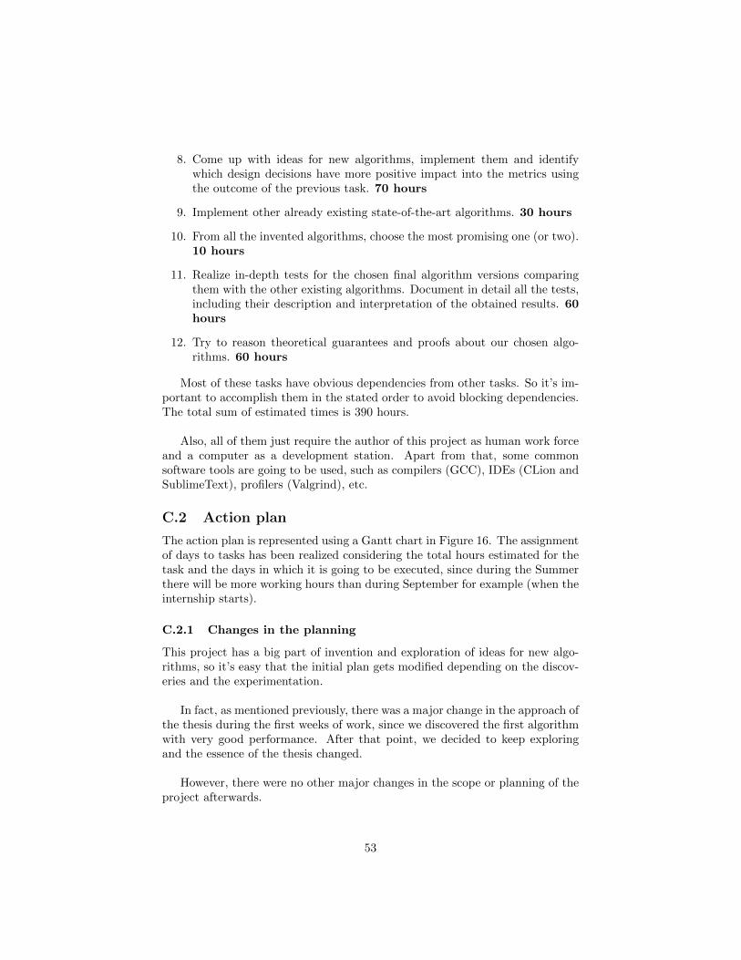
8. Come up with ideas for new algorithms, implement them and identifywhich design decisions have more positive impact into the metrics usingthe outcome of the previous task. 70 hours
9. Implement other already existing state-of-the-art algorithms. 30 hours
10. From all the invented algorithms, choose the most promising one (or two).10 hours
11. Realize in-depth tests for the chosen final algorithm versions comparingthem with the other existing algorithms. Document in detail all the tests,including their description and interpretation of the obtained results. 60hours
12. Try to reason theoretical guarantees and proofs about our chosen algo-rithms. 60 hours
Most of these tasks have obvious dependencies from other tasks. So it’s im-portant to accomplish them in the stated order to avoid blocking dependencies.The total sum of estimated times is 390 hours.
Also, all of them just require the author of this project as human work forceand a computer as a development station. Apart from that, some commonsoftware tools are going to be used, such as compilers (GCC), IDEs (CLion andSublimeText), profilers (Valgrind), etc.
C.2 Action plan
The action plan is represented using a Gantt chart in Figure 16. The assignmentof days to tasks has been realized considering the total hours estimated for thetask and the days in which it is going to be executed, since during the Summerthere will be more working hours than during September for example (when theinternship starts).
C.2.1 Changes in the planning
This project has a big part of invention and exploration of ideas for new algo-rithms, so it’s easy that the initial plan gets modified depending on the discov-eries and the experimentation.
In fact, as mentioned previously, there was a major change in the approach ofthe thesis during the first weeks of work, since we discovered the first algorithmwith very good performance. After that point, we decided to keep exploringand the essence of the thesis changed.
However, there were no other major changes in the scope or planning of theproject afterwards.
53
Figure 16: Gantt chart of the project. High resolution: https://goo.gl/GiQoJN
There was a minor delay in the initial planning because some tests were notpossible to be executed in a local machine, since they required a lot of resourcesof memory and CPU. Hence, we had to move the development environment toan EC2 instance of Amazon Web Services in order to run the tests with therequired resources cheaply.
There were no other deviations of the initial planning.
54

D Budget and sustainability
This work is a scientific research project, so it is not very straightforward toanalyze it, regarding the economic impact, as a regular business activity. Thisis because it is practically impossible to estimate the costs in which other busi-nesses incur using similar algorithms, and also to estimate the cost of the newones. However, some analysis is possible and has positive results to all the im-plicated parties from an environmental, economic and social points of views.There hasn’t been any changes from the initial prevision.
D.1 Environmental impact
The goal of this project is to find algorithms more efficient and accurate thanthe existing ones, which are extensively used in many areas as we already sawin previous chapters. This kind of algorithms are used without interruptionon these industries, since they analyze very large or unbounded streams. Soa small optimization in them will imply an important save of computationalresources consumption. This will translate to less electricity usage, so a smallerenvironmental footprint. So in case they are adopted by the industry, theirenvironmental impact will be positive, since they will decrease other business’footprint.
However, during the phase of the design and the experimentation of thenew algorithms, some environmental resources will be used, and again, they aremainly electricity. Thanks to the nature of software this will be a fixed expense,and after this work is finished, the use of these algorithms will only save otherresources, and it will easily compensate this initial consumption.
Anyways, a prediction of this initial environmental resources consumptionis required. In order to obtain it, we will use the number of estimated requiredhours to develop this project calculated on previous chapters. Apart from thosehuman-working hours, we also have to consider all the time required for runningthe tests and experiments, which is notably a lot. The sum of those hours, withthe estimated hourly consumption of electricity by a personal computer will bethe prediction of used electricity.
It’s difficult to estimate the required amount of hours to run the tests, butI expect to run a test every night of the second half of the development of thisproject. Following the Gantt chart, this means that I will start with this timeconsuming tests in September-October, during 105 days. These tests consist onstreams of one hundred million elements approximately, and they usually last 7hours.
Testing hours =Estimated project days
2
7 hours
night= 367 hours
55

Computing hours = Working hours + Testing hours = 390 + 367 = 757 hours
Electricity = Computing hours ·Mean power consumption
= 757 hours · 0.1 kW = 75.7 kWh
Regarding physical resources, I will use my personal computer without need-ing any additional hardware. So in this sense, there will be no footprint comingfrom buying new hardware.
D.2 Economic impact
As discussed previously, it’s difficult to elaborate a detailed analysis of the eco-nomic impact of the project on its useful life. But anyways, we can detail abudget (based on the estimated costs) to realize this investigation project.
The main cost of this project will come from the human working hours,which is a direct cost. More specifically, from the student and professor au-thors of this thesis. The amount of hours spent by the student will be the onesdetailed on the previous chapter: 390. The hours spent by the professor willbe estimated as 1/8 of the student hours, ie approximately 49 hours, since hewill have to actively review the work done by the student, discuss new ideas, etc.
Then, considering an hourly salary of 25 euros for the student, and 50 forthe professor, we get a direct cost of:
Direct cost = 390 hours · 25 euros
hour+ 49 hours · 50 euros
hour= 12200 euros
The only indirect economic expense will be related to the consumption ofelectricity. This, at the same time, will depend on the hours required to developthe algorithms and to run the experiments. From the environmental analy-sis, we know the total expected consumption of electricity, and we will use thatmetric with the mean hourly cost of electricity to estimate the economic impact.
Indirect cost = 75.7 kWh · 0.07 euros
kWh= 5.3 euros
Then, we can calculate the total costs as:
Total estimated cost = 12200 euros + 5.3 euros = 12205.30 euros
And adding a 8% of that quantity as contingency costs, we get as finalbudget:
Total budget = Total estimated cost · 1.08 = 13185.54 euros
56
D.3 Social impact
Depending on the use of the algorithms proposed in this project, the social im-pact will be different. The algorithms solve a theoretical problem present indata streams, and as we saw on previous chapters, this problem can be foundin very different real situations. These algorithms aim to solve more accuratelythe problem, so the entities using them in a future will be able to get betterresults. That can translate to detecting better DDoS attacks, or decreasing thelatency of Internet services. So in theory this project will have a positive socialimpact (although very indirectly) to possibly many people.
From a personal perspective, the authors of this project will expand theirknowledge and skills. If the proposed algorithms turn out to be successful, theymay receive recognition from other researchers.
57

References
[1] A. Helmi, J. Lumbroso, C. Martınez, and A. Viola. “Data Streams as Ran-dom Permutations: the Distinct Element Problem”. In N. Broutin and L.Devrye, editors. Proc. 23rd Int. Conf. on Probabilistic, Combinatorial andAsymptotic Methods for the Analysis of Algorithms (AofA). Discrete Mathe-matics & Theoretical Computer Science (Proceedings), pages 323–338, 2012.https://hal.inria.fr/hal-01197221/document
[2] A. Metwally, D. Agrawal, and A. E. Abbadi. “Efficient Computation ofFrequent and Top-k Elements in Data Streams”. In International Conferenceon Database Theory, pages 398–412, 2005.https://pdfs.semanticscholar.org/72f1/5aba2e67b1cc9cd1fb12c99e101c4c1aae4b.pdf
[3] E. Demaine, A. Lopez-Ortiz, and J. Munro. “Frequency Estimation ofInternet Packet Streams with Limited Space”. In Proceedings of the 10th
ESA Annual European Symposium on Algorithms, pages 348–360, 2002.https://pdfs.semanticscholar.org/ab52/1e91a2bce4fd13326cba9a765b479feefd61.pdf
[4] M. Charikar, K. Chen, and M. Farach-Colton. “Finding Frequent Items inData Streams”. In Proceedings of the 29th ICALP International Colloquiumon Automata, Languages and Programming, pages 693–703, 2002.https://www.cs.rutgers.edu/∼farach/pubs/FrequentStream.pdf
[5] G. Cormode and S. Muthukrishnan. “An improved data stream summary:The count-min sketch and its applications”. In Journal of Algorithms,55(1):58–75, 2005.http://dimacs.rutgers.edu/ graham/pubs/papers/cm-full.pdf
[6] G. Manku and R. Motwani. “Approximate Frequency Counts over DataStreams”. In Proceedings of the 28th ACM VLDB International Conferenceon Very Large Data Bases, pages 346–357, 2002.http://www.vldb.org/conf/2002/S10P03.pdf
[7] M. Fischer and S. Salzberg. “Finding a Majority Among N Votes: Solutionto Problem 81-5”. In Journal of Algorithms, 3:376–379, 1982.http://citeseerx.ist.psu.edu/viewdoc/summary?doi=10.1.1.56.3439
[8] L. Devroye. “Non-Uniform Random Variate Generation”. In Springer-Verlag, New York, 1986.http://www.nrbook.com/devroye/
58